DESY 00-082
June 2000
Inflation and Supersymmetry Breaking

Abstract

We study the connection between inflation and supersymmetry breaking in the context of an O’Raifeartaigh model which can account for both hybrid inflation and a true vacuum where supersymmetry is spontaneously broken. For a weakly coupled inflaton field, the dynamics during the inflationary phase can be determined by the supersymmetry breaking scale $M_{S}\sim 10^{10}\,\mbox{GeV}$, even if $H_{I}\gg m_{3/2}$. The spectrum of density fluctuations is then almost scale invariant, with a spectral index $n-1={\cal O}(M_{G}^{2}/M_{\rm P}^{2})$. The mass parameter $M_{G}$ of the O’Raifeartaigh model is determined by the COBE normalization for the cosmic microwave background to be the grand unification scale, $M_{G}\sim 10^{16}\,\mbox{GeV}$.

It is well known that an inflationary phase in the early history of the universe can explain its present flatness, isotropy and homogeneity [1]. From the COBE measurement of the cosmic microwave background (CMB) anisotropy it has soon been realized that the scale of inflation has to be lower than the Planck scale, but much larger than the electroweak scale. It is therefore clear that supersymmetry may play an important role for inflation. Many models have been proposed describing an inflationary phase in the context of globally supersymmetric theories [2]. But since supersymmetry is not exact in nature, we know that globally supersymmetric models can give us only an approximate description of the real world. Supergravity corrections can strongly affect the inflationary phase [3], and a variety of models have been constructed in a general supergravity framework [2]. However, it is often thought that, when the scale of inflation is much larger than the supersymmetry breaking scale, a globally supersymmetric model is sufficiently accurate to describe the inflationary phase as well as the reheating process.

As we shall see, this is not the case. The goal of this paper is to study explicitly a model containing both, supersymmetry breaking in the true vacuum and during the inflationary phase . On the one hand, in such a case the supersymmetry breaking sector is influenced by the inflaton dynamics, and the true vacuum is reached only at the end of inflation. On the other hand, also the inflationary potential is modified by the presence of the supersymmetry breaking sector. This modification turns out to be very important in the case of a weakly coupled inflaton field.

In the following we first describe the model, which combines a Fayet term [5] for global symmetry breaking with a Polonyi term [6] for supersymmetry breaking, leading to a particular O’Raifeartaigh model [7]. We then analyze the model without and with supergravity corrections. Finally, we briefly discuss the moduli problem and the reheating process.

The model

The usual hybrid inflation scenario is based on a superpotential of the type

$$W_{G}=\lambda T\left(M_{G}^{2}-\Sigma^{2}\right)\;,$$ (1)

where $T$ and $\Sigma$ are chiral superfields. Such a potential is well-known and has initially been used [5] to break global or local symmetries in supersymmetric theories. Apart from being the simplest choice giving hybrid inflation [3],[8]-[12], it has also the advantage of avoiding large supergravity corrections in the case of a canonical Kähler potential. This is due to the fact that the superpotential is linear in the inflaton field $T$. In (1) higher powers of $T$ are forbidden by R-invariance.

To the potential (1) we add, as supersymmetry breaking part, the Polonyi potential

$$W_{S}=M_{S}^{2}(\beta+S)\;,$$ (2)

with $\beta=(2-\sqrt{3})M_{\rm P}$, which allows for supersymmetry breaking in the true vacuum where $\langle S\rangle=(\sqrt{3}-1)M_{\rm P}$. $M_{S}$ is the scale of supersymmetry breaking yielding the gravitino mass $m_{3/2}=M_{S}^{2}/M_{\rm P}\exp(2-\sqrt{3})$ and $M_{\rm P}=(8\pi G_{N})^{-1/2}=2.4\cdot 10^{18}\,\mbox{GeV}$. For numerical estimates we shall use $m_{3/2}\simeq 100$ GeV, which corresponds to the supersymmetry breaking scale $M_{S}\simeq 1.4\cdot 10^{10}$ GeV.

In the case of global supersymmetry the scalar Polonyi potential is flat,

$$V_{S}=\left|{\partial W_{S}\over\partial S}\right|^{2}=M_{S}^{4}\;.$$ (3)

This has motivated early attempts to identify the Polonyi field $S$ with the inflaton field [13]. However, supergravity corrections turn out to be too large and spoil the flatness of the potential.

The constant $\beta$ in the Polonyi potential (2) is only relevant in the supergravity framework. It breaks R-invariance, and it is adjusted to have vanishing cosmological constant. As we shall see, this constant may play an important role during inflation. Our conclusions will generally apply to any supersymmetry breaking effective potential where the constant and the linear term dominate in an expansion in powers of $S$.

Combining the two superpotentials (1) and (2) we arrive at

$$W=W_{G}+W_{S}=\lambda T\left(M_{G}^{2}-\Sigma^{2}\right)+M_{S}^{2}\left(\beta+S\right)\;.$$ (4)

Further, we choose the canonical Kähler potential for the fields $T,\Sigma$ and $S$. Note, that the superpotential (4) is a particular O’Raifeartaigh model. This becomes apparent after a change of variables. Defining

$$\Phi={\xi\,S\over\sqrt{1+\xi^{2}}}+{T\over\sqrt{1+\xi^{2}}}\;,\quad\Psi={S\over\sqrt{1+\xi^{2}}}-{\xi\,T\over\sqrt{1+\xi^{2}}}\;,$$ (5)

with $\xi=M_{S}^{2}/(\lambda M_{G}^{2})$, and

$$\lambda_{1}={\lambda\over\sqrt{1+\xi^{2}}}\;,\quad\lambda_{2}={\lambda\,\xi\over\sqrt{1+\xi^{2}}}\;,\quad M=M_{G}\sqrt{1+\xi^{2}}\;,$$ (6)

one obtains

$$W=\lambda_{1}\Phi(M^{2}-\Sigma^{2})+\lambda_{2}\Psi\Sigma^{2}+M_{S}^{2}\beta\;.$$ (7)

This is the more familiar form of an O’Raifeartaigh model [7]. The two superpotentials (4) and (7) are equivalent, and in the following we will use one or the other according to our convenience. As we shall see, successful inflation requires $\xi$ to be very small, so that effectively $T\simeq\Phi$, $S\simeq\Psi$ and $M\simeq M_{G}$.

Hybrid inflation

For global supersymmetry the scalar potential reads

$$V_{G}+V_{S}=\lambda^{2}|M_{G}^{2}-\Sigma^{2}|^{2}+4\lambda^{2}|T|^{2}|\Sigma|^{2}+M_{S}^{4}\;,$$ (8)

and the corresponding ground state is given by

$$\langle T\rangle=0\;,\quad\langle\Sigma\rangle=M_{G}\;,$$ (9)

while $\langle S\rangle$ is undetermined. Hence, the supersymmetry breaking sector decouples, and an inflationary phase can take place as in ordinary hybrid inflation, starting with a large value of $T$. The field $\Sigma$ is then pushed to the origin by a large mass term and the potential is perfectly flat along $T$. A small curvature needed for the ‘slow roll’ is generated by the quantum corrections due to the loops of the $\Sigma$ particles [9], which are non-vanishing since supersymmetry is broken by $F_{T}=\partial W_{G}/\partial T\neq 0$. The corresponding one-loop correction to the scalar potential reads,

$$\Delta V_{G}={\lambda^{4}M_{G}^{4}\over 8\pi^{2}}\left(\ln(2\lambda^{2}\phi^{2}/\mu^{2})+O(M^{4}_{G}/\phi^{4})\right)\;,$$ (10)

where $\phi$ is the real part of the complex scalar field $T$ and $\mu$ is a renormalization scale.

Inflation ends at $\phi_{c}\simeq M_{G}$, where the mass of $\Sigma$ becomes negative and the field acquires a non-vanishing expectation value. For $M_{S}\ll\lambda^{1/2}M_{G}$, the potential (10) satisfies the slow-roll conditions [2] down to $\phi_{c}$,

$$\epsilon = {M_{\rm P}^{2}\over 2}\left({V^{\prime}\over V}\right)^{2}={\lambda^{4}\over 32\pi^{4}}{M_{\rm P}^{2}\over\phi^{2}}\ll 1\;,$$ (11)

$$\eta = M_{\rm P}^{2}{V^{\prime\prime}\over V}=-{\lambda^{2}\over 4\pi^{2}}{M_{\rm P}^{2}\over\phi^{2}}\ ,\quad|\eta|\ll 1\;,$$ (12)

as long as $\lambda$ is of order $M_{G}/M_{\rm P}$.

The number of e-folds between the inflaton field value $\phi$ and the end of inflation at $\phi_{c}$ is given by

$$N(\phi)=\int_{t(\phi_{c})}^{t(\phi)}H_{I}dt=\int_{\phi_{c}}^{\phi}{V\over V^{\prime}}d\phi={2\pi^{2}\over\lambda^{2}}{\phi^{2}-\phi^{2}_{c}\over M_{\rm P}^{2}}\;,$$ (13)

where $t$ denotes time and $H_{I}\simeq\sqrt{V_{G}/(3M_{\rm P}^{2})}\simeq\lambda M^{2}_{G}/(\sqrt{3}M_{\rm P})$ in the slow-roll approximation.

Adiabatic density perturbations originate as vacuum fluctuations during inflation. The COBE normalization [14] then gives

$$\delta_{H}\equiv{1\over\sqrt{75}\pi M_{\rm P}^{3}}{V_{*}^{3/2}\over|V_{*}^{\prime}|}={4\pi\over\sqrt{75}}{M_{G}^{2}\phi_{*}\over\lambda M_{\rm P}^{3}}=1.94\times 10^{-5}\;,$$ (14)

where the $*$ indicates that the potential and its derivative are evaluated at the epoch of horizon exit for the comoving scale $k_{*}\simeq 10H_{0}$ [14]. Defining $N_{*}$ as the number of e-folds at that epoch, the corresponding inflaton value is given by $\phi_{*}/M_{\rm P}\simeq\sqrt{\lambda^{2}N_{*}/(2\pi^{2})+\phi^{2}_{c}/M_{\rm P}^{2}}$. We thus obtain the relation

$${M^{2}_{G}\over M_{\rm P}^{2}}\left(N_{*}+{2\pi^{2}\over\lambda^{2}}{\phi_{c}^{2}\over M_{\rm P}^{2}}\right)^{1/2}\simeq 5.9\cdot 10^{-5}\;,$$ (15)

where the number of e-folds is $N_{*}\simeq 50$.

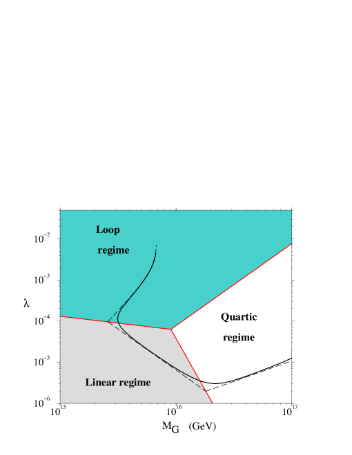
Figure 1: The three regimes of hybrid inflation: the loop regime, the linear regime and the quartic regime. The COBE normalization defines a curve (full line) in the $\lambda-M_{G}$ - plane. The dashed lines are obtained by assuming approximate forms of the inflaton potential as discussed in the text.

From eq. (15) one reads off that a consistent picture is obtained for $M_{G}/M_{\rm P}\sim\lambda\sim 10^{-3}$, with $H_{I}\sim 10^{-8}M_{\rm P}$. The exact relation between $\lambda$ and $M_{G}$ imposed by the COBE constraint is shown in fig. (1). It is interesting that $M_{G}$ is naturally of order the grand unification scale. Moreover, due to the smallness of $\lambda$ the observable number of e-folds corresponds to inflaton fields $\phi$ close to the critical value $\phi_{c}\simeq M_{G}\ll M_{\rm P}$.

Supergravity corrections

Let us now consider the effect of the supersymmetry breaking Polonyi potential and of corrections suppressed by powers of $1/M_{\rm P}$. The supergravity scalar potential reads

$$V=e^{K/M_{\rm P}^{2}}\left[\left|{\partial W\over\partial z_{i}}+{z_{i}^{*}W\over M_{\rm P}^{2}}\right|^{2}-3{|W|^{2}\over M_{\rm P}^{2}}\right]\;,$$ (16)

where the sum extends over all fields $z_{i}$, and $K$ is chosen to be the canonical Kähler potential, $K=\sum_{i}|z_{i}|^{2}$.

The additional non-renormalizable terms modify slightly the vacuum expectation values of the fields $T$ and $\Sigma$ and give a large expectation value to the Polonyi field $S$. Since the corrections to the derivatives of the superpotential are always proportional to $\langle W\rangle/M_{\rm P}^{2}\ll 1$, it is possible to expand the potential in powers of $M_{S}\over M_{\rm P}$. This yields for the first corrections to the vacuum expectation values,

$$\langle\Sigma\rangle = M_{G}\left[1+\frac{2-\sqrt{3}}{4}\frac{M_{S}^{4}}{\lambda^{2}M_{\rm P}^{2}M_{G}^{2}}+O\left({M_{S}^{3}\over M_{\rm P}^{3}}\right)\right]\;,$$ (17)

$$\langle T\rangle = {1\over 2\lambda}{M_{S}^{2}\over M_{\rm P}}+O\left({M_{S}^{3}\over M_{\rm P}^{2}}\right)\;.$$ (18)

Also the value of $\beta$, which is adjusted to have vanishing cosmological constant, and the vacuum expectation value of $S$ acquire corrections,

$$\langle S\rangle = (\sqrt{3}-1)M_{\rm P}-\frac{9-4\sqrt{3}}{24}\frac{M_{S}^{4}}{\lambda^{2}M_{\rm P}^{3}}\;,$$ (19)

$$\beta = (2-\sqrt{3})M_{\rm P}-\frac{\sqrt{3}}{6}\frac{M_{G}^{2}}{M_{\rm P}}\;.$$ (20)

Clearly, all corrections ${\cal O}(1/M_{\rm P}^{n})$ to the vacuum expectation values are very small. One may therefore be tempted to think that also during the inflationary phase supergravity corrections are practically negligible. This, however, is not the case.

During the inflationary phase $\Sigma$ is driven to zero by the large value of $T$. The potential is then most easily computed in the basis $\Phi,\Psi$. Neglecting the one-loop correction, one has

$$V = \lambda^{2}M_{G}^{4}\left(1+\xi^{2}-{2\sqrt{2}\xi\beta\varphi\over M_{\rm P}^{2}}-{\xi^{2}\beta^{2}(\varphi^{2}+\chi^{2})\over M_{\rm P}^{4}}-{\xi\beta\varphi^{3}\over\sqrt{2}M_{\rm P}^{4}}-{\sqrt{2}\xi\beta\varphi\chi^{2}\over M_{\rm P}^{4}}\right.$$ (21)

$$\hskip 56.9055pt\left.+{(\varphi^{2}+\chi^{2})^{2}\over 8M_{\rm P}^{4}}+{|\Psi|^{2}\over M_{\rm P}^{2}}\left(1+{\varphi^{2}+\chi^{2}\over 2M_{\rm P}^{2}}\right)+\ldots\right)\;,$$

where $\xi=M^{2}_{S}/(\lambda M^{2}_{G})\ll 1$ and $\Phi=(\varphi+i\chi)/\sqrt{2}$. Here we have neglected terms which are small for values of $\Phi$ in the range $1>|\Phi|\gg\xi$. Note, that the potential for $\Phi$ at $\Psi=0$ is just the Polonyi potential, but with the ‘wrong’ constant $\xi\beta$, i.e. while the supersymmetry breaking scale during inflation is given by $\lambda^{1/2}M_{G}$, the constant is still related to the supersymmetry breaking scale $M_{S}$ in the true vacuum. The hierarchy between the two scales is exactly what makes the potential flat enough, contrary to the simple expectation for the Polonyi potential with only one scale of supersymmetry breaking. This hierarchy also implies that in the potential (21) the term linear in $\varphi$ is larger than the $\varphi$ mass term, which is suppressed by an additional power of $\xi$.

We remark that in the case of a charged inflaton field, or in general when the superpotential contains only second and higher powers of the inflaton field, no linear term is generated by the supersymmetry breaking sector. Then the first supergravity correction is a mass term and inflation can be realized even with $H\simeq m_{3/2}$, if the inflaton mass is sufficiently suppressed either by cancelations or by the running mass mechanism [15].

The minimum of the potential (21) with respect to $\Psi$ and $\chi$ lies at the origin, but it is very flat. However, for initial values $\varphi={\cal O}(M_{\rm P})$ one can have $m_{\Psi},m_{\chi}>H$, which may be sufficient to drive $\Psi$ and $\chi$ to the origin before the beginning of inflation. In the following we shall assume $\Psi\simeq\chi\simeq 0$ as initial conditions.

Comparing (21) with (10) it is clear that the standard hybrid inflation scenario may be significantly modified depending on the values of $\lambda$ and $M_{G}$. The one-loop radiative corrections dominate over the linear term in (21) for $\lambda^{2}/(2\pi)^{2}\geq\xi\beta\varphi/(\sqrt{2}M_{\rm P}^{2})$. Substituting $\beta/M_{\rm P}=2-\sqrt{3}$ and using $\varphi>\varphi_{c}\geq M_{G}$, one obtains the lower bound on $\lambda$,

$$\lambda>3\left({M_{S}^{2}\over M_{G}M_{\rm P}}\right)^{1/3}\;.$$ (22)

For the hybrid inflation value $M_{G}\simeq 3\cdot 10^{-3}M_{\rm P}$, this yields $\lambda>0.7\cdot 10^{-4}$. As discussed above, hybrid inflation takes place in the vicinity of $\varphi_{c}$. For couplings $\lambda$ above the lower bound the one-loop radiative corrections also dominate over the supergravity induced quartic term in (21). Hence, for $M_{G}\simeq 3\cdot 10^{-3}M_{\rm P}$ and couplings in the range

$$0.7\cdot 10^{-4}<\lambda<6\cdot 10^{-3}$$ (23)

the standard hybrid inflation scenario is only weakly affected by supergravity corrections.

Scale invariant inflation

Consider now the case of small couplings,

$$\lambda<3\left({M_{S}^{2}\over M_{G}M_{\rm P}}\right)^{1/3}\;,$$ (24)

for which the linear term in (21) dominates over the one-loop radiative corrections (cf. fig. 1). From the COBE normalization (14) one then obtains, independently of $N_{*}$,

$$\delta_{H}={1\over\sqrt{75}\pi M_{\rm P}^{3}}{V_{*}^{3/2}\over|V_{*}^{\prime}|}={1\over 2\sqrt{150}\pi}{M_{S}^{2}\over\xi^{2}\beta M_{\rm P}}\simeq 1.9\cdot 10^{-5}\;.$$ (25)

Fixing $M_{S}\simeq 1.4\cdot 10^{10}\,\mbox{GeV}$, this implies $\xi\equiv M^{2}_{S}/(\lambda M_{G}^{2})\simeq 5\cdot 10^{-7}$. Note, that $\xi$ is the ratio of the gravitino masses in the true vacuum and in the inflationary phase. Since $\xi\ll 1$, a huge number of e-folds is generated near $\varphi_{c}=-M_{G}$,

$$N(\phi)=-{M_{G}\over 2\sqrt{2}\,\xi\beta}\,{\varphi-\varphi_{c}\over\varphi_{c}}\;,$$ (26)

which include the cosmologically relevant scales with $N\simeq 50$. The linear term dominates over the quartic term in (21) if $|\varphi^{3}|/(2M_{\rm P}^{2})<2\sqrt{2}\xi\beta$. Together with (25), this yields an upper bound on $M_{G}$. Similarly, a lower bound on $M_{G}$ follows from (24). Inserting numerical values for $\xi$ and $M_{S}$ one finds that the linear term dominates in the range

$$2\cdot 10^{15}\mbox{GeV}<M_{G}<2\cdot 10^{16}\mbox{GeV}\;.$$ (27)

The slow-roll conditions are clearly satisfied for $\varphi\simeq\varphi_{c}$,

$$\epsilon = {4\xi^{2}\beta^{2}\over M_{\rm P}^{2}}\left(1-{\varphi^{3}\over 2\sqrt{2}\xi\beta M_{\rm P}^{2}}+\ldots\right)\ \ll 1\;,$$ (28)

$$\eta = {3\over 2}{\varphi^{2}\over M_{\rm P}^{2}}+\ldots\ \ll 1\;.$$ (29)

Here we have kept the quartic supergravity correction to the linear term in (21), which affects the spectral index,

$$n-1\simeq 3{\varphi_{*}^{2}\over M_{\rm P}^{2}}\leq 2.4\cdot 10^{-4}\;.$$ (30)

An inflationary phase dominated by a linear term is very interesting, since it gives a scale invariant spectrum to high accuracy. For standard hybrid inflation, on the contrary, one has $n\simeq 0.98$ [9]. Future satellite experiments may eventually be able to distinguish between these two versions of hybrid inflation.

The linear term in the potential breaks the symmetry $\varphi\rightarrow-\varphi$. (cf. fig. 2). For negative $\varphi$ hybrid inflation can take place, as discussed above. The potential has a Polonyi-type minimum at $\varphi_{min}\simeq(4\sqrt{2}\xi\beta/M_{\rm P})^{1/3}M_{\rm P}\simeq 9\cdot 10^{-3}M_{\rm P}$. For positive initial condition hybrid inflation can take place as long as $M_{G}>\varphi_{min}$. Otherwise, the inflaton field is trapped at $\varphi_{min}$. Inflation then continues in this metastable state and has to terminate in a different way.

Let us finally turn to the case where the quartic term dominates during inflation, a possibility already considered in [16]. This occurs for $M_{G}>2\cdot 10^{16}$ GeV. The slow-roll conditions,

$$\epsilon = {\varphi^{6}\over 4M_{\rm P}^{6}}\left(1-{2\sqrt{2}\xi\beta M_{\rm P}^{2}\over\varphi^{3}}+...\right)\ll 1\;,$$ (31)

$$\eta = {3\over 2}{\varphi^{2}\over M_{\rm P}^{2}}+\ldots\ll 1\;,$$ (32)

are satisfied for field values small compared to $M_{\rm P}$. The number of e-folds is given by

$$N(\varphi)=\int_{\varphi_{c}}^{\varphi}d\varphi{2M_{\rm P}^{2}\over\varphi^{3}}={M_{\rm P}^{2}\over\varphi_{c}^{2}}-{M_{\rm P}^{2}\over\varphi^{2}}\;.$$ (33)

For $\varphi_{c}<10^{-1}M_{\rm P}$ the cosmologically relevant scales again correspond to $\varphi_{*}\simeq\varphi_{c}$.

The COBE normalization determines $\lambda$ as function of $M_{G}$ (cf. fig. 1), with $\lambda>3\cdot 10^{-6}$. For the spectral index one obtains

$$n-1\simeq 3{\varphi_{*}^{2}\over M_{\rm P}^{2}}\geq 2.4\cdot 10^{-4}\;.$$ (34)

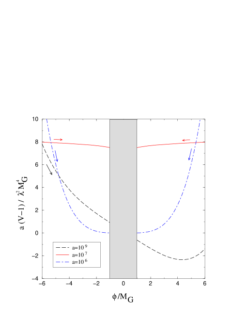
Figure 2: The full inflaton potential for three sets of parameters $(\lambda,M_{G})$: $(10^{-3},5\cdot 10^{15}\,\mbox{GeV})$, $(1.5\cdot 10^{-5},5\cdot 10^{15}\,\mbox{GeV})$ and $(4\cdot 10^{-6},4\cdot 10^{16}\,\mbox{GeV})$, corresponding to the loop regime (dotted line), the linear regime (dashed line) and the quartic regime (dashed-dotted line), respectively. The flattest potential is obtained in the linear regime (Note the different rescaling factors!). The arrows indicate the directions of possible inflationary phases.

The three regimes of hybrid inflation, the loop regime, the linear regime and the quartic regime, are summarized in fig. 1. The COBE normalization defines a curve in the $\lambda-M_{G}$ - plane. The dashed lines are obtained by assuming that a single term dominates the derivative of the supergravity potential. The full line is based on the full potential. Increasing (decreasing) the scale of supersymmetry breaking $M_{S}$ shifts the curve in the linear regime, as well as the boundaries, to larger (smaller) values of $\lambda$. The inflaton potentials in the three regimes are compared in fig. 2. Note, that the flattest potential corresponds to the linear regime.

Moduli problem and reheating

At the end of the inflationary period the field $\Sigma$ has to change from $0$ to $M_{G}$, the field $T$ from $M_{G}$ to $M_{S}^{2}/(2\lambda M_{\rm P})$ and the field $S$ from $0$ to $(\sqrt{3}-1)M_{\rm P}$. As in the usual Polonyi model S acquires a small mass $m_{S}\sim m_{3/2}$ in the true vacuum, like the standard model fields which have only gravitational interactions with $S$. The late decays of $S$ are then incompatible with nucleosynthesis, which is the so-called cosmological moduli problem [17].

Several ways have been proposed to circumvent the moduli problem. For instance, it does not occur if the amplitude of the moduli field is reduced via an effective mass term during the evolution to the true vacuum [18]. This can be implemented in the present model by adding the following non-renormalizable term to the superpotential,

$$W_{M}\equiv\frac{\alpha}{M_{\rm P}}S^{2}T^{2}\;.$$ (35)

This interaction is negligible during inflation, where $S\ll M_{\rm P}$, and modifies only slightly the expectation values in the true vacuum.

However, at the end of inflation, $T\simeq M_{G}$ and $S$ acquires the mass $m_{S}=2\alpha M_{G}^{2}/M_{\rm P}$. The amplitude of the S field oscillations is then sufficiently damped for $m_{S}\gg H_{I}=\lambda M_{G}^{2}/(\sqrt{3}M_{\rm P})$ [18]. This is the case for $\alpha\gg\lambda$, which can be easily satisfied.

The interaction (35) also induces a large mass for the T field, $m_{T}\sim\alpha M_{\rm P}\gg\lambda M_{G}$, when $S$ approaches its minimum. $T$ then decays rapidly to other particles. The computation of the corresponding reheating temperature is not straightforward, since it depends on the dynamics of the field $S$. A detailed analysis of this process, including the thermal and non-thermal production of gravitinos, is in progress. A rough estimate, providing a lower bound on the reheating temperature, can be obtained by considering the decay of $\Sigma$ into quarks. Supergravity always induces the non-renormalizable couplings

$${\cal L}=Y_{q}QHq{|\Sigma|^{2}\over M_{\rm P}^{2}}\;,$$ (36)

where $Y_{q}$ is the quark Yukawa coupling, $Q$ ($q$) the quark doublet (singlet) and $H$ the corresponding Higgs doublet. From the top-quark contribution alone, one obtains a reheating temperature $T_{R}\sim 10^{6}\,\mbox{GeV}$ [1]. Clearly, this simple picture may be strongly modified by additional interactions.

Finally, let us comment on the possible production of topological defects at the end of inflation. The potential (4) has a $Z_{2}$ symmetry with respect to the field $\Sigma$, that would give rise to domain walls at the end of inflation [19]. In order to avoid them, it is sufficient, either to consider higher order non-renormalizable terms breaking the $Z_{2}$ symmetry or, like in many formulations of hybrid inflation, give to the $\Sigma$ field a charge under a gauge group and substitute $\Sigma^{2}$ by $\Sigma\bar{\Sigma}$ or $Tr(\Sigma^{2})$, depending on the gauge group representation. In the last case, at the end of inflation other topological defects could arise, e.g. strings, and could give a non-negligible contribution to the density perturbations [20].

Conclusions

We have studied in detail the connection between inflation and supersymmetry breaking in the context of an O’Raifeartaigh model, which can account for both a hybrid inflationary phase and a true vacuum where supersymmetry is spontaneously broken. Crucial ingredients of the model are two contributions to the superpotential: a term linear in the inflaton field and a constant which is required by the nearly vanishing cosmological constant in the true vacuum. This constant generates a linear and higher order terms in the inflaton field. This does not spoil the flatness of the inflaton potential since the energy scale during inflation turns out to be large compared to the scale of supersymmetry breaking. For the same reason the linear term in the inflaton potential dominates over the mass term.

The dynamics during the inflationary phase depends on the size of the Yukawa coupling in the O’Raifeartaigh model. For $\lambda>10^{-4}$, the usual picture of hybrid inflation driven by loop corrections applies. However, for smaller coupling $\lambda<10^{-4}$, and $M_{G}<2\times 10^{16}\,\mbox{GeV}$, the linear term in the effective potential dominates the evolution of the inflaton field. As a consequence, the spectrum of fluctuations is almost scale invariant. The deviation of the spectral index from one is determined by the mass parameter $M_{G}$ of the O’Raifeartaigh model, $n-1={\cal O}(M_{G}^{2}/M_{\rm P}^{2})$. It is remarkable that for $M_{S}\sim 10^{10}\,\mbox{GeV}$ the COBE normalization for the cosmic microwave background determines $M_{G}$ to be the unification scale, $M_{G}\sim 10^{16}\,\mbox{GeV}$.

We would like to thank D. H. Lyth for clarifying comments.

References

- [1] E. W. Kolb and M. S. Turner, The Early Universe, Addison-Wesley (1990)
-
[2]
For a review and references, see
D. H. Lyth, A. Riotto, Phys. Rep. 314C (1999) 1 - [3] E. J. Copeland, A. R. Liddle, D. H. Lyth, E. D. Stewart, D. Wands, Phys. Rev. D 49 (1994) 6410
-
[4]
L. Randall, M. Soljacic and A. Guth, Nucl. Phys. B 472 (1996) 377;
A. Riotto, Nucl. Phys. B 515 (1998) 413;
K.-I. Izawa, Prog. Theor. Phys. 99 (1998) 157 - [5] P. Fayet, Nucl. Phys. B 90 (1975) 104
- [6] J. Polonyi, Budapest preprint KFKI-93 (1977)
- [7] L. O’Raifeartaigh, Nucl. Phys. B 96 (1975) 331
- [8] A. D. Linde, Phys. Lett. B 259 (1991) 38
- [9] G. Dvali, Q. Shafi, R. K. Schaefer, Phys. Rev. Lett. 73 (1994) 1886
- [10] G. Lazarides, R. K. Schaefer, Q. Shafi, Phys. Rev. D 56 (1997) 1324
- [11] A. D. Linde and A. Riotto, Phys. Rev. D 56 (1997) 1841
- [12] T. Asaka, K. Hamaguchi, M. Kawasaki, T. Yanagida, Phys. Rev. D 61 (2000) 083512
- [13] B. A. Ovrut and P. J. Steinhardt, Phys. Lett. B 133 (1983) 161
- [14] E. F. Bunn, M. White, Astrophys. J. 480 (1997) 6.
-
[15]
E. D. Stewart, Phys. Lett. B 391 (1997) 34, Phys. Rev. D 56 (1997) 2019;
L. Covi, D. H. Lyth, Phys. Rev. D 59 (1999) 063515;
L. Covi, D. H. Lyth, L. Roszkowski, Phys. Rev. D 60 (1999) 023509 - [16] A. D. Linde, Phys. Rev. D 49 (1994) 748; D. Roberts, A. R. Liddle and D. H. Lyth, Phys. Rev. D 51 (1995) 4122
- [17] G. D. Coughlan, W. Fischler, E. W. Kolb, S. Raby, G. G. Ross, Phys. Lett. B 131 (1983) 59
- [18] A. D. Linde, Phys. Rev. D 53 (1996) R4129
- [19] Ya. B. Zel’dovich, I. Yu. Kobzarev and L. B. Okun, Sov. Phys.-JETP 40 (1975) 1
- [20] C. Contaldi, M. Hindmarsh and J. Magueijo, Phys. Rev. Lett. 82 (1999) 2034