Report of the Beyond the MSSM Subgroup for the Tevatron Run II SUSY/Higgs Workshop

Abstract

There are many low-energy models of supersymmetry breaking parameters which are motivated by theoretical and experimental considerations. Some of these approaches have gained more proponents than others over time, and so have been studied in greater detail. In this contribution we discuss some of the lesser-known theories of low-energy supersymmetry, and outline their phenomenological consequences. In some cases, these theories have more gauge symmetry or particle content than the Minimal Supersymmetric Standard Model. In other cases, the parameters of the Lagrangian are unusual compared to commonly accepted norms (e.g., Wino LSP, heavy gluino LSP, light gluino, etc.). The phenomenology of supersymmetry varies greatly between the different models. Correspondingly, particular aspects of the detectors assume greater or lesser importance. Detection of supersymmetry and the determination of all parameters may well depend upon having the widest possible view of supersymmetry phenomenology.

I Introduction

Most of the studies performed to assess the discovery reach for supersymmetry and most of the current limits on the masses of supersymmetric particles have been obtained assuming R-parity conservation, the minimal matter content of the Minimal Supersymmetric Model (MSSM), and universal boundary conditions at $M_{U}$ for the soft-SUSY-breaking parameters: $m_{0}$ for the scalar masses; $M_{0}$ for the SU(3),SU(2) and U(1) gaugino masses $M_{3,2,1}$; and $A_{0}$ for the tri-linear scalar field couplings. Additional parameters of the MSSM include: $\tan\beta$, the ratio of Higgs field vacuum expectation values $\langle H_{u}\rangle/\langle H_{d}\rangle$; $\mu$, the coefficient of the bilinear $\widehat{H}_{u}\widehat{H}_{d}$ superpotential term; and $B$, which specifies the strength of the corresponding $H_{u}H_{d}$ scalar field mixing term. By requiring correct electroweak symmetry breaking after evolution down to the scale $m_{Z}$, the magnitude of $\mu$ is fixed and only its sign remains undetermined. This boundary condition scenario is often referred to as the mSUGRA or CMSSM model. If unification of the $\tau$ and $b$ Yukawa couplings at $M_{U}$ is required, then correct EWSB strongly constrains $\tan\beta$ as well.

Table 1: Parameter count in the SM and MSSM extensions: BV=baryon-number violating; LV=lepton-number violating; BLV=both B and L violating.

	masses and	CP-violating
model	mixing angles	phases	TOTAL
Standard Model	17	2	19
(MSSM)RPV	79	45	124
(MSSM)${}_{\rm BV\phantom{L}}$	97	62	159
(MSSM)${}_{\rm LV\phantom{B}}$	157	122	279
(MSSM)BLV	175	140	315

While the matter content and boundary conditions of the MSSM have the virtue of simplicity and can be reasonably motivated in the context of several types of gravity-mediated supersymmetry breaking, other possibilities should certainly be considered. For a model with MSSM matter content and R-parity conservation, the most general form of soft-SUSY-breaking allows for a total of 124 parameters (not counting certain additional parameters expected to be suppressed by $1/M_{U}$ factors). This is to be compared to the 19 parameters of the Standard Model. The most general form of R-parity violation increases the parameter count to 315. Some of these parameters are associated with phases and CP violation. A summary appears in Table LABEL:paramcount. A final parameter is the mass of the gravitino, $\widetilde{G}$. If the scale of supersymmetry breaking is sufficiently low, $m_{\widetilde{G}}$ can be small enough that it is the LSP. In particular, this is the expectation in models where supersymmetry breaking is mediated by gauge interactions.

Although almost all of the most general parameter space is excluded by various phenomenological constraints (no FCNC, proton stability, small EDM’s, etc.), there are sub-spaces that differ drastically from mSUGRA while maintaining consistency with all existing data. Examples include models with R-parity violation and the standard GMSB phenomenology, both of which will be covered in separate reports. We also do not consider non-zero phases. Aside from a discussion of the phenomenology of an extremely light $\widetilde{G}$, our focus will be on models with a heavy $\widetilde{G}$ and soft-SUSY-breaking parameters that conserve R-parity and CP. Even with these restrictions, there are many well-motivated theories with MSSM matter content that yield vastly different phenomenology than the mSUGRA model. In addition, we will consider a number of models in which the matter/gauge content of the MSSM is extended. We will focus in particular on implications for supersymmetry discovery and study at the upgraded Tevatron.

We now give brief motivation and an introduction to the models considered.

• One of the least satisfactory features of the MSSM is the ad hoc nature of the parameter $\mu$, which a priori is most naturally of order $M_{U}$, but which is expected to be $\;\raise 1.29167pt\hbox{$<$\kern-7.5pt\raise-4.73611pt\hbox{$\sim$}}\;1\hbox{\rm\,TeV}$ for natural EWSB. The addition of a singlet superfield $\widehat{S}$ provides a very compelling and natural origin of the $\mu\widehat{H}_{u}\widehat{H}_{d}$ superpotential term. Such a term arises if the scalar component of $\widehat{S}$ ($S$) acquires a vacuum expectation value. The result is an effective superpotential interaction of the form $\langle S\rangle\widehat{H}_{u}\widehat{H}_{d}$. The $S$ quantum degrees of freedom result in 1 CP-even and 1 CP-odd Higgs bosons beyond the 2 CP-even and 1 CP-odd Higgs bosons of the MSSM. The spin-1/2 component of $\widehat{S}$ provides an additional neutralino, $\widetilde{S}$, that can mix with the usual four neutralinos of the MSSM. It is very natural for the LSP of this model to be the $\widetilde{S}$. All supersymmetric particles then cascade decay down to the $\widetilde{S}$. The phenomenology of SUSY detection is then significantly altered compared to mSUGRA. A review of this phenomenology is given in Sec. II.

• In mSUGRA, the LSP is essentially always a light bino-like neutralino, $\widetilde{\chi}^{0}_{1}\sim\widetilde{B}$. However, there is substantial motivation for the possibility that the LSP is a massive gluino. This occurs if $M_{3}\ll M_{1,2}$, as is possible in several well-motivated SUSY-breaking scenarios. Current limits on a heavy gluino LSP are summarized and discovery prospects are discussed in Sec. III.

• Another alternative arrangement of the gaugino masses that arises in string and brane models is $M_{2}<M_{1}<M_{3}$. In this case, the LSP $\widetilde{\chi}^{0}_{1}$ is wino-like and is highly degenerate with the lightest chargino. (This assumes $|\mu|$ is large, as usually implied by RGE EWSB.) The resulting phenomenology differs greatly from mSUGRA phenomenology. If $\Delta m_{\widetilde{\chi}}\equiv m_{\widetilde{\chi}^{\pm}_{1}}-m_{\widetilde{\chi}^{0}_{1}}$ is not too much larger than $m_{\pi}$, striking background-free signals for $\widetilde{\chi}^{+}_{1}\widetilde{\chi}^{-}_{1}+\widetilde{\chi}^{\pm}_{1}\widetilde{\chi}^{0}_{1}$ production will be present. For $\Delta m_{\widetilde{\chi}}\;\raise 1.29167pt\hbox{$>$\kern-7.5pt\raise-4.73611pt\hbox{$\sim$}}\;300\hbox{\rm\,MeV}$, detection of these processes will be very difficult; one will have to hope that other SUSY particles are light. Section IV gives a discussion of the phenomenology and of some very critical detector issues and related discovery strategies.

• Although the scalar masses have the universal value $m_{0}$ at the high scale, significant flavor violation can arise via RGE evolution if this scale is not the same as $M_{U}$. More generally, FCNC will be a problem unless the SUSY breaking mechanism yields either universality for the scalar masses or flavor alignment. An interesting exception to this statement is the possibility that the scalar masses for all the sfermions of the first two generations are simply extremely heavy ($>10\hbox{\rm\,TeV}$) and, thus, have greatly suppressed FCNC effects. Very heavy scalars are also helpful for unifying with greater precision the strong coupling constant with the SU(2) and U(1) couplings for the somewhat ‘low’ value, $\alpha_{s}(m_{Z})\sim 0.12$, preferred by existing data. Of course, to maintain naturalness for the Higgs sector the 3rd generation squarks should be below $\sim 1\hbox{\rm\,TeV}$. This scenario is sometimes referred to as Superheavy Supersymmetry or More Minimal Supersymmetry. Section V reviews some theoretical issues and constraints on this scenario, including the apparent necessity to have GMSB-like boundary conditions in order to preserve anomaly cancellations.

• As noted earlier, the mass of the $\widetilde{G}$ is another crucial parameter of supersymmetry. If $m_{\widetilde{G}}$ is very small, the couplings of the $\widetilde{G}$ are sufficiently large that processes in which the $\widetilde{G}$ is directly produced have observable rates. Since the $\widetilde{G}$ is undetectable, the most basic signature is jets plus missing energy. If these processes are detected, they provide a measurement of the scale of supersymmetry breaking, possibly the most important parameter of supersymmetry. The phenomenology and discovery prospects for direct production of a very light $\widetilde{G}$ are reviewed in Sec. VI.

• An interesting question is whether superstring theory provides any guidance as regards boundary conditions and matter content for low energy supersymmetry. The detailed predictions of one sample superstring model are outlined in Sec. VII. The model considered has a plethora of additional matter, including exotics, extra Higgs bosons, and extra gauge bosons. This provides further warning against being complacent in our approach to SUSY phenomenology.

• The possibility that left-right symmetry is restored at a high energy scale is very attractive. In LR-symmetric models, proper symmetry breaking requires introduction of triplet Higgs representations that contain a doubly-charged Higgs field. In the supersymmetric context, these doubly-charged scalars have a doubly-charged higgsino partner. Careful investigation reveals that these are likely to be one of the lightest states in the superparticle spectrum. They will appear in cascade decays and can also be directly produced. The phenomenology of the doubly-charged higgsino states is reviewed in Sec. VIII.

• Recently, the possibility that the compactified extra dimensions of the string/brane world are large and that the Kaluza-Klein excited states are within experimental reach has received much attention. Some of the indirect signals for such extra dimension are reviewed in Sec. IX. In addition, Sec. VI considers external KK gravitons production, which provides a signature similar to that of the very light gravitino through jets plus missing energy.

• It is well-known that supersymmetry predicts a rather low mass for the lightest CP-even Higgs boson. Thus, one should ask whether supersymmetry can be rescued if a sufficiently light Higgs boson is not discovered. One means for increasing the upper bound on the light Higgs is to introduce a 4th family. The contraints upon and implications for the Higgs sector of supersymmetry in a 4-family model are discussed in Sec. X.

• Is there room for a 4th family in supersymmetry? If the Yukawa couplings associated with the 4th family are to remain perturbative in evolving from $\sim m_{Z}$ up to some high scale, one finds that the leptons and quarks of the 4th family must be quite light. Experimental constraints are becoming very restrictive. In Sec. XI, the current situation is reviewed with the conclusion that the 4th generation will almost certainly be either discovered or eliminated as a possibility during Run II at the Tevatron.

• Could the gluino be very light? Remarkably, this scenario cannot yet be absolutely excluded. In addition, it might explain some detailed features of Run I jet data at very high $p_{T}$. Section XII presents the case for a very light gluino.

• The DØ detector has been upgraded dramatically for Run II. It is important to understand the extent to which it will be able to probe some of the more exotic supersymmetry scenarios that are discussed here and elsewhere. Particularly interesting are signals associated with long-lived charged particles, photons, vertices etc. The capabilities of the DØ detector as regards such exotic phenomena are discussed in Sec. XIII.

• The other major detector at the Tevatron, CDF, has also been upgraded. Section XIV reviews its capabilities for 4th generation searches via: looking for a long-lived ($b^{\prime}$) parent of the $Z$; looking for prompt $b^{\prime}\rightarrow bZ$ production; and searching for a long-lived heavy quark or similar object.

• New gauges bosons are a common feature of supersymmetric models motivated by string theory. The ability to detect such gauge bosons and to determine their couplings during Run II at the Tevatron is considered in Section XV

• We end with some brief concluding remarks in Section XVI.

II Cascade decays in the NMSSM

U. Ellwanger and C Hugonie

The NMSSM (Next-to-minimal SSM, or (M+1)SSM) is defined by the addition of a gauge singlet superfield $S$ to the MSSM. The superpotential $W$ is scale invariant, i.e. there is no $\mu$-term. Instead, two Yukawa couplings $\lambda$ and $\kappa$ appear in $W$. Apart from the standard quark and lepton Yukawa couplings, $W$ is given by

$$W=\lambda H_{1}H_{2}S+\frac{1}{3}\kappa S^{3}+\ldots$$ (1)

and the corresponding trilinear couplings $A_{\lambda}$ and $A_{\kappa}$ are added to the soft susy breaking terms. The vev of $S$ generates an effective $\mu$-term with $\mu=\lambda\langle S\rangle$.

The constraint NMSSM (CNMSSM) ell1 is defined by universal soft susy breaking gaugino masses $M_{0}$, scalar masses $m_{0}^{2}$ and trilinear couplings $A_{0}$ at the GUT scale, and a number of phenomenological constraints:

- Consistency of the low energy spectrum and couplings with negative Higgs and sparticle searches.

- In the Higgs sector, the minimum of the effective potential with $\langle H_{1}\rangle$ and $\langle H_{2}\rangle\neq 0$ has to be deeper than any minimum with $\langle H_{1}\rangle$ and/or $\langle H_{2}\rangle=0$. Charge and colour breaking minima induced by trilinear couplings have to be absent. (However, deeper charge and colour breaking minima in ”UFB” directions are allowed, since the decay rate of the physical vacuum into these minima is usually large compared to the age of the universe ell2 .)

Cosmological constraints as the correct amount of dark matter are not imposed at present. (A possible domain wall problem due to the discrete $Z_{3}$ symmetry of the model is assumed to be solved by, e.g., embedding the $Z_{3}$ symmetry into a $U(1)$ gauge symmetry at $M_{GUT}$, or by adding non-renormalisable interactions which break the $Z_{3}$ symmetry without spoiling the quantum stability ell3 .)

The number of free parameters of the CNMSSM, ($M_{1/2}$, $m_{0}$, $A_{0}$, $\lambda$, $\kappa$ + standard Yukawa couplings), is the same as in the CMSSM ($M_{1/2}$, $m_{0}$, $A_{0}$, $\mu$, $B+\ idem$). The new physical states in the CNMSSM are one additional neutral Higgs scalar and Higgs pseudoscalar, respectively, and one additional neutralino. In general these states mix with the corresponding ones of the MSSM with a mixing angle proportional to the Yukawa coupling $\lambda$. However, in the CNMSSM $\lambda$ turns out to be quite small, $\lambda\;\raise 1.29167pt\hbox{$<$\kern-7.5pt\raise-4.73611pt\hbox{$\sim$}}\;0.1$ (and $\lambda\ll 1$ for most allowed points in the parameter space) ell1 Thus the new physical states are generally almost pure gauge singlets with very small couplings to the standard sector.

The new states in the Higgs sector can be very light, a few GeV or less, depending on $\lambda$ ell4 . Due to their small couplings to the $Z$ boson they will escape detection at LEP and elsewhere, i.e. the lightest “visible” Higgs boson is possibly the next-to-lightest Higgs of the NMSSM. The upper limits on the mass of this visible Higgs boson (and its couplings) are, on the other hand, very close to the ones of the MSSM, i.e. $\;\raise 1.29167pt\hbox{$<$\kern-7.5pt\raise-4.73611pt\hbox{$\sim$}}\;140$ GeV depending on the stop masses ell4 .

The phenomenology of sparticle production in the CNMSSM can differ considerably from the MSSM, depending on the mass of the additional state $\tilde{S}$ in the neutralino sector: If the $\tilde{S}$ is not the LSP, it will hardly be produced, and all sparticle decays proceed as in the MSSM with a LSP in the final state. If, on the other hand, the $\tilde{S}$ is the LSP, the sparticle decays will proceed differently: First, the sparticles will decay into the NLSP, because the couplings to the $\tilde{S}$ are too small. Only then the NLSP will realize that it is not the true LSP, and decay into the $\tilde{S}$ plus an additional cascade.

The condition for a singlino LSP scenario can be expressed relatively easily in terms of the bare parameters of the CNMSSM: Within the allowed parameter space of the CNMSSM, the lightest non-singlet neutralino is essentially a bino $\tilde{B}$. Since the masses of $\tilde{S}$ and $\tilde{B}$ are proportional to $A_{0}$ and $M_{1/2}$, respectively, one finds, to a good approximation, that the $\tilde{S}$ is the true LSP if the bare susy breaking parameters satisfy $|A_{0}|\;\raise 1.29167pt\hbox{$<$\kern-7.5pt\raise-4.73611pt\hbox{$\sim$}}\;0.4M_{1/2}$. Since $A_{0}^{2}\;\raise 1.29167pt\hbox{$>$\kern-7.5pt\raise-4.73611pt\hbox{$\sim$}}\;9m_{0}^{2}$ is also a necessary condition within the CNMSSM, the singlino LSP scenario corresponds essentially to the case where the gaugino masses are the dominant soft susy breaking terms.

Note, however, that the $\tilde{B}$ is not necessarily the NLSP in this case: Possibly the lightest stau $\tilde{\tau}_{1}$ is lighter than the $\tilde{B}$, since the lightest stau can be considerably lighter than the sleptons of the first two generations. Nevertheless, most sparticle decays will proceed via the $\tilde{B}\rightarrow\tilde{S}+\ldots$ transition, which will give rise to additional cascades with respect to decays in the MSSM. The properties of this cascade have been analysed in ell5 , and in the following we will briefly discuss the branching ratios and the $\tilde{B}$ life times in the different parameter regimes:

a) $\tilde{B}\rightarrow\tilde{S}\nu\bar{\nu}$: This invisible process is mediated dominantly by sneutrino exchange. Since the sneutrino mass, as the mass of $\tilde{B}$, is essentially fixed by $M_{1/2}$ ell5 , the associated branching ratio varies in a predictable way with $M_{\tilde{B}}$: It can become up to 90% for $M_{\tilde{B}}\sim 30$ GeV, but decreases with $M_{\tilde{B}}$ and is maximally 10% for $M_{\tilde{B}}\;\raise 1.29167pt\hbox{$>$\kern-7.5pt\raise-4.73611pt\hbox{$\sim$}}\;65$ GeV.

b) $\tilde{B}\rightarrow\tilde{S}l^{+}l^{-}$: This process is mediated dominantly by the exchange of a charged slepton in the s-channel. If the lightest stau $\tilde{\tau}_{1}$ is considerably lighter than the sleptons of the first two generations, the percentage of taus among the charged leptons can well exceed $\frac{1}{3}$. If $\tilde{\tau}_{1}$ is lighter than $\tilde{B}$, it is produced on-shell, and the process becomes $\tilde{B}\rightarrow\tilde{\tau}_{1}\tau\rightarrow\tilde{S}\tau^{+}\tau^{-}$. Hence we can have up to 100% taus among the charged leptons and the branching ratio of this channel can become up to 100%.

c) $\tilde{B}\rightarrow\tilde{S}S$: This two-body decay is kinematically allowed if both $\tilde{S}$ and $S$ are sufficiently light. (A light $S$ is not excluded by Higgs searches at LEP1, if its coupling to the $Z$ is too small ell4 .) However, the coupling $\tilde{B}\tilde{S}S$ is proportional to $\lambda^{2}$, whereas the couplings appearing in the decays a) and b) are only of $O(\lambda)$. Thus this decay can only be important for $\lambda$ not too small. In ell5 , we found that its branching ratio can become up to 100% in a window $10^{-3}\;\raise 1.29167pt\hbox{$<$\kern-7.5pt\raise-4.73611pt\hbox{$\sim$}}\;\lambda\;\raise 1.29167pt\hbox{$<$\kern-7.5pt\raise-4.73611pt\hbox{$\sim$}}\;10^{-2}$. Of course, $S$ will decay immediately into $b\bar{b}$ or $\tau^{+}\tau^{-}$, depending on its mass. (If the branching ratio $Br(\tilde{B}\rightarrow\tilde{S}S)$ is substantial, $S$ is never lighter than $\sim 5$ GeV.) If the singlet is heavy enough, its $b\bar{b}$ decay gives rise to 2 jets with $B$ mesons, which are easily detected with $b$-tagging. In any case, the invariant mass of the $b\bar{b}$ or the $\tau^{+}\tau^{-}$ system would be peaked at $M_{S}$, making this signature easy to search for.

d) $\tilde{B}\rightarrow\tilde{S}\gamma$: This branching ratio can be important if the mass difference $\Delta M=M_{\tilde{B}}-M_{\tilde{S}}$ is small ($\;\raise 1.29167pt\hbox{$<$\kern-7.5pt\raise-4.73611pt\hbox{$\sim$}}\;5$ GeV).

Further possible final states like $\tilde{B}\rightarrow\tilde{S}q\bar{q}$ via $Z$ exchange have always branching ratios below 10%. (The two-body decay $\tilde{B}\rightarrow\tilde{S}Z$ is never important, even if $\Delta M$ is larger than $M_{Z}$: In this region of the parameter space $\tilde{\tau}_{1}$ is always the NLSP, and thus the channel $\tilde{B}\rightarrow\tilde{\tau}_{1}\tau$ is always preferred.)

The $\tilde{B}$ life time depends strongly on the Yukawa coupling $\lambda$, since the mixing of the singlino $\tilde{S}$ with gauginos and higgsinos is proportional to $\lambda$. Hence, for small $\lambda$ (or a small mass difference $\Delta M$) the $\tilde{B}$ can be so long lived that it decays only after a macroscopic length of flight $l_{\tilde{B}}$. An approximate formula for $l_{\tilde{B}}$ (in meters) is given by

$$l_{\tilde{B}}[m]\simeq 2\cdot 10^{-10}\frac{1}{\lambda^{2}\cdot M_{\tilde{B}}[GeV]}\ ,$$ (2)

and $l_{\tilde{B}}$ becomes $>\ 1$ mm for $\lambda\;\raise 1.29167pt\hbox{$<$\kern-7.5pt\raise-4.73611pt\hbox{$\sim$}}\;6\cdot 10^{-5}$.

To summarize, the following unconventional signatures are possible within the CNMSSM, compared to the MSSM:

a) additional cascades attached to the original vertex (but still missing energy and momentum): one or two additional $l^{+}l^{-}$, $\tau^{+}\tau^{-}$ or $b\bar{b}$ pairs or photons, with the corresponding branching ratios depending on the parameters of the model.

b) one or two additional $l^{+}l^{-}$ or $\tau^{+}\tau^{-}$ pairs or photons with macroscopically displaced vertices, with distances varying from millimeters to several meters. These displaced vertices do not point towards the interaction point, since an additional invisible particle is produced.

More details on the allowed branching ratios and life times can be found in ell5 , applications to sparticle production processes et LEP 2 are published in ell6 , and differential (spin averaged) cross sections of the $\tilde{B}\rightarrow\tilde{S}$ decay are available upon request.

III Report on the gluino-LSP scenario

H Baer, K. Cheung, J.F. Gunion

III.1 Introduction

This contribution will present a brief overview of the results of Ref. bcg . Most GUT scale boundary conditions (e.g. the mSUGRA universal boundary conditions in which the gaugino masses are assumed to have a common value at $M_{U}$) lead to the gluino being much heavier than the lightest neutralino. However, there are several models in which the gluino is heavy but is yet the lightest supersymmetric particle, denoted $\widetilde{g}$-LSP.
     (a) A $\widetilde{g}$-LSP can arise in models in which the gaugino masses are given by one-loop corrections plus a contribution from Green-Schwarz mixing (parameterized by $\delta_{GS}$) nonuniv ; guniondrees2 . An example is the O-II string model in the limit where all SUSY breaking arises from the size-modulus field and none from the dilaton. At $M_{U}$ one has:

$$M_{3}:M_{2}:M_{1}\stackrel{{\scriptstyle\scriptstyle O-II}}{{\sim}}-(3+\delta_{GS}):(1-\delta_{GS}):({33\over 5}-\delta_{GS})\,,$$ (3)

and after evolution down to 1 TeV or below a heavy gluino is the LSP when $\delta_{GS}\sim-3$ (a preferred range for the model).
     (b) In the GMSB context, the possibility of a heavy $\widetilde{g}$-LSP has been stressed in Ref. raby . In the model constructed, the $\widetilde{g}$ is the LSP as a result of mixing between the Higgs fields and the messenger fields.

In fact, there are three significant indications that a light gluino is to be preferred over the universal gaugino mass result of $m_{\widetilde{g}}\sim 7m_{\widetilde{\chi}^{0}_{1}}$.

$\bullet$ The first such hint relates to the magnitude of $\alpha_{s}$ predicted by requiring precise gauge coupling unification at $M_{U}\sim 10^{16}~{}{\rm GeV}$. For universal masses at $M_{U}$, gauge coupling unification typically requires $\alpha_{s}(m_{Z})\sim 0.125-0.13$ when sparticle masses are $\mathrel{\raise 1.29167pt\hbox{$<$\kern-7.5pt\lower 4.30554pt\hbox{$\sim$}}}1~{}{\rm TeV}$, a value that is uncomfortably high relative to the best fit value of $\alpha_{s}(m_{Z})\mathrel{\raise 1.29167pt\hbox{$<$\kern-7.5pt\lower 4.30554pt\hbox{$\sim$}}}0.12$. Although unified gauge couplings at $M_{U}$ can be made consistent with $\alpha_{s}(m_{Z})\mathrel{\raise 1.29167pt\hbox{$<$\kern-7.5pt\lower 4.30554pt\hbox{$\sim$}}}0.12$ if the sparticle masses important in the gauge coupling running are all $\mathrel{\raise 1.29167pt\hbox{$>$\kern-7.5pt\lower 4.30554pt\hbox{$\sim$}}}10~{}{\rm TeV}$ (for which fine tuning is regarded as a problem), a much more interesting possibility is that discussed in Ref. lrshif . There it is shown that if the gluino mass is substantially below, or at least comparable to the $\widetilde{\chi}^{\pm}_{1}$ mass (these determine the two most critical thresholds in gauge coupling running), then $\alpha_{s}(m_{Z})\mathrel{\raise 1.29167pt\hbox{$<$\kern-7.5pt\lower 4.30554pt\hbox{$\sim$}}}0.12$ is much easier to achieve.

$\bullet$ The second hint is from fine tuning. As discussed most recently in Ref. kaneking , the most severe problem in fine tuning arises from the fact that the magnitude of the standard measure of fine tuning contains a term proportional to $M_{3}^{2}(M_{U})$ with a very large numerical coefficient, much larger than the (possibly canceling) terms proportional to $M_{1}^{2}(M_{U})$ and $M_{2}^{2}(M_{U})$. (Very roughly, the relative size of these coefficients are determined by the relative size of the corresponding gauge couplings squared, although $\tan\beta$ is also an important ingredient.) The fine tuning problem is greatly relaxed if $M_{3}(M_{U})$ is substantially smaller than $M_{1,2}(M_{U})$. For example, using the $\tan\beta=2.5$ numerical coefficients given in kaneking , one measure of fine tuning is (all parameters at $M_{U}$ with $\widehat{M}_{i}$ and $\widehat{m}_{i}$ denoting $M_{i}(M_{U})/m_{Z}$ and $m_{i}(M_{U})/m_{Z}$)

$$\Delta_{\mu}\sim 23.8\widehat{M}_{3}^{2}-1.3\widehat{M}_{2}^{2}+0.01\widehat{M}_{1}^{2}+1.66\widehat{M}_{2}\widehat{M}_{3}+0.206\widehat{M}_{1}\widehat{M}_{3}+0.045\widehat{M}_{1}\widehat{M}_{2}+\ldots\,,$$ (4)

Since the $\widehat{M}_{2}^{2}$ coefficient is not very large, taking $\widehat{M}_{3}=0$ (leading to a gluino LSP) avoids significant fine-tuning problems. One can even arrange for the $\widehat{M}_{3}$ and $\widehat{M}_{2}$ terms to cancel ($\widehat{M}_{3}\sim\widehat{M}_{2}/5$). Thus, the $\widehat{M}_{3}$ values predicted for O-II model boundary conditions in the favored $\delta_{GS}\sim-3,-4,-5$ range would lead to a considerable relaxation of the the fine tuning problem and a gluino that is much lighter than normally anticipated.

$\bullet$ The third hint relates to vacuum stability. This has been recently reviewed in Ref. cim , where references to earlier work can be found. The most serious problem associated with many of the soft-supersymmetry-breaking boundary conditions motivated by string theory is the presence of directions in field space for which the effective potential is unbounded from below (UFB). Dangerous charge and color breaking (CCB) minima are also possible. The strongest constraint typically arises from the UFB-3 direction, which involves the fields $H_{2},\nu_{L_{i}},e_{L_{j}},e_{R_{j}}$ with $i\neq j$. After minimizing the effective potential, the latter three fields can be expressed in terms of $H_{2}$. The value of the potential in the UFB-3 direction is then given by:

$$V_{UFB-3}=(m^{2}_{H_{2}}+m_{L_{i}}^{2})|H_{2}|^{2}+{|\mu|\over\lambda_{e_{j}}}(m_{L_{j}}^{2}+m_{e_{j}}^{2}+m_{L_{i}}^{2})|H_{2}|-{2m_{L_{i}}^{4}\over g^{\prime\,2}+g^{2}}\,,$$ (5)

where $\lambda_{e_{j}}$ is the leptonic Yukawa coupling of the $j$-th generation. We must have $V_{UFB-3}(Q=\widehat{Q})>V_{\rm real~{}min}=-{1\over 8}(g^{\prime\,2}+g^{2})(v_{2}^{2}-v_{1}^{2})^{2}$, where $\widehat{Q}\sim{\rm Max}\left[\lambda_{\rm top}|H_{2}|,m_{\widetilde{t}}\right]$. The problem arises when $m_{H_{2}}^{2}$ is negative (as happens under RGE electroweak symmetry breaking) and is most restrictive for $j=3$ for which $\lambda_{e_{j}}$ is largest. One finds that any significant amount of supersymmetry breaking from the dilaton leads to violation of the condition. The modulus-dominated (or one-loop) limit boundary conditions of Eq. 3 (or extremely close thereto) open up some allowed parameter space. This happens as follows. The RGE for $m_{H_{2}}^{2}$ is (using $t=\ln(Q)$) $dm_{H_{2}}^{2}/dt=12(\lambda_{\rm top}/4\pi)^{2}m_{\widetilde{t}}^{2}+\ldots$. The smaller $m_{\widetilde{t}}$, the less negative $m_{H_{2}}^{2}$ is driven in evolving down from $M_{U}$, and, since

$${dm_{\widetilde{q}}^{2}\over dt}=\left({1\over 2\pi}\right)\left(-{16\over 3}M_{3}^{2}\alpha_{3}+\ldots\right)\,,$$ (6)

smaller $M_{3}$ implies smaller $m_{\widetilde{t}}$. Meanwhile, the positive terms in Eq. (5) have evolution

$${dm_{e}^{2}\over dt}=\left({1\over 2\pi}\right)\left(-{12\over 5}M_{1}^{2}\alpha_{1}+\ldots\right)\,,\quad{dm_{L}^{2}\over dt}=\left({1\over 2\pi}\right)\left(-3M_{2}^{2}\alpha_{2}-{3\over 5}M_{1}^{2}\alpha_{1}+\ldots\right)\,,$$ (7)

implying larger $m_{e}^{2}$ and $m_{L}^{2}$ in $V_{UFB-3}$ for larger $M_{1,2}$. Thus, non-universal boundary conditions with small $M_{3}$ relative to $M_{1,2}$ are crucial in the string model context and, more generally, are quite useful in satisfying the UFB-3 constraint.

It is often stated that a stable $\widetilde{g}$-LSP is ruled out by virtue of relic density constraints, especially the non-observation of anomalous isotopes. However, such constraints are inevitably model dependent. In Ref. bcg it is shown that if the annihilation cross section for gluinos is nonperturbatively enhanced near threshold (many models of this type exist) then the relic density of gluinos could be very small. If, in addition, they did not cluster with nucleons (e.g. if they are concentrated at galaxy cores), then relic constraints would not rule out this scenario. Alternatively, the reheating required to avoid the Polonyi problem would also effectively eliminate the relic gluinos. It is also possible that the gluino could decay but with a lifetime so long that it is effectively stable in the detector. This is possible if there is a very weak violation of R-parity or in gauge-mediated-SUSY-breaking (GMSB) models where $\widetilde{g}\rightarrow g\widetilde{G}$ (where the $\widetilde{G}$ is the gravitino) can be very suppressed by a large supersymmetric breaking scale. Thus, it is important to consider how to place constraints on a detector-stable gluino (for which we use the generic $\widetilde{g}$-LSP notation) using accelerator experiments. We will focus on constraints that arise by looking directly for the $\widetilde{g}$’s themselves. That is, we do not include processes where other supersymmetric particles are produced and then decay into $\widetilde{g}$’s.

III.2 Behavior of a $\widetilde{g}$-LSP in a Detector

As soon as a $\widetilde{g}$-LSP is produced in a detector, it picks up a gluon or quark-antiquark combination to form an ‘R-hadron’; $R^{0}=\widetilde{g}g$ is likely to be the lightest state, but color-singlet $\widetilde{g}q^{\prime}\overline{q}$ states could have very similar mass, and if the difference in mass between such states and the $R^{0}$ were $<m_{\pi}$ they would be pseudo-stable in the detector. The behavior of a $\widetilde{g}$-LSP in a typical detector depends very much upon whether the dominant R-hadron fragment is charged (probability $P$) or neutral (probability $1-P$). Simple quark counting models suggest that $P<1/2$. The important ingredients in determining the energy deposited by the $\widetilde{g}$-LSP in the detector are:

• the hadronic interaction length, $\lambda_{T}$, as determined by $\sigma_{T}$;

• the average energy deposited per hadronic collision, $\langle\Delta E\rangle$, as a function of the $\widetilde{g}$’s velocity;

• the amount of ionization energy deposited between hadronic interactions and how the calibrated detector measures this energy;

• the thickness (measured most conveniently by the number of hadronic interaction lengths) of various components of the detector.

One should picture the $\widetilde{g}$-LSP as emerging from the hard production process as a neutral (charged) R-hadron with probability $1-P$ ($P$). At each hadronic interaction the light quarks and gluons are presumed to be stripped away and the $\widetilde{g}$-LSP again fragments into a neutral or charged R-hadron with probability $1-P$ or $P$, respectively. Thus, for any $P\neq 0,1$, the charge of the R-hadron between hadronic collisions fluctuates. In Ref. bcg , several models for $\lambda_{T}$ (i.e. for the $\widetilde{g}$-LSP total cross section) and for $\langle\Delta E\rangle$ are considered. For the most likely case of $P<1/2$, one finds that the energy deposited by the $\widetilde{g}$-LSP is dominated by hadronic energy deposits rather than by ionization energy deposits. Further, for $P<1/2$ only a small fraction of the gluino’s energy is actually deposited. The $\widetilde{g}$-LSP behaves like a bowling ball moving through a sea of ping-pong balls. The result is that the $\widetilde{g}$-LSP generally exits the detector, thereby leading to missing energy aligned with a soft jet. For processes of interest, the $\widetilde{g}$’s are always produced in pairs and are seldom back to back. As a result, the net missing energy is usually large and not aligned with any one of the jets observed in the detector. Thus, the crucial signal for $P<1/2$ is jets + missing energy. This signal is also generally quite useful even for $P>1/2$ since the momentum of a $\widetilde{g}$-jet is never properly determined even if the energy deposited via ionization is large. (In fact, the ionization energy deposit is generally overestimated, and for $P\sim 1$ the ‘measured’ gluino momentum can even exceed its true momentum in the OPAL analysis procedure used later.)

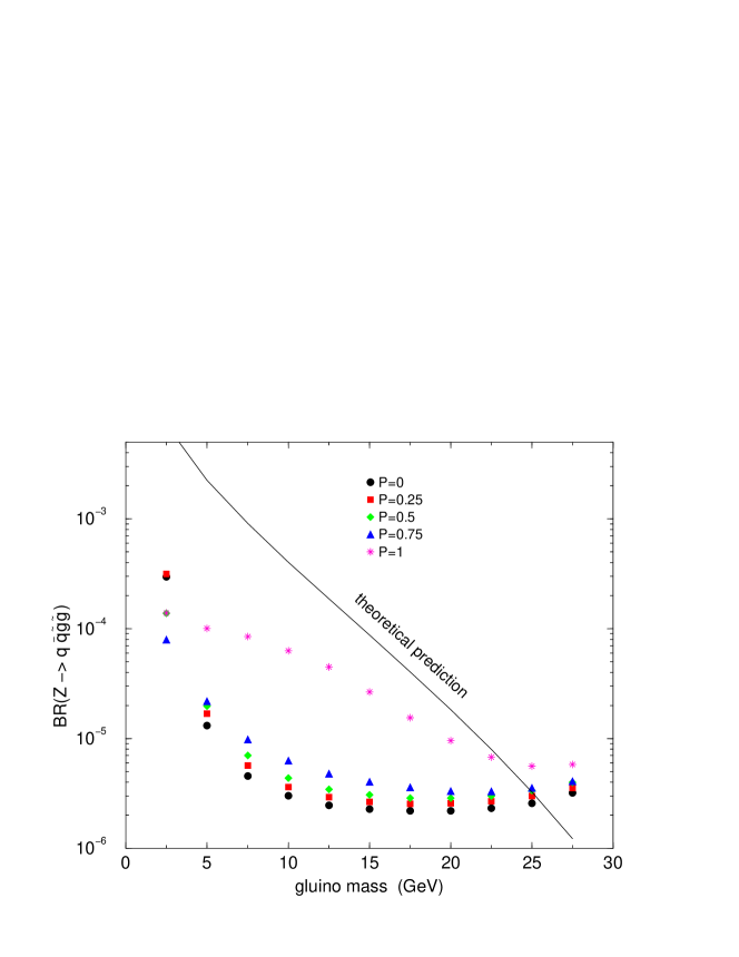
Figure 1: We consider $q\overline{q}\widetilde{g}\widetilde{g}$ for $P=0,1/4,1/2,3/4,1$ using event-by-event determination of the measured $\widetilde{g}$ jet energies. For $P\neq 0,1$, changes of the $R$-hadron charge as it passes through the detector are randomly implemented. Both smearing and fragmentation effects are included. The figure gives, as a function of $m_{\widetilde{g}}$, the OPAL 95% CL upper limits compared to the theoretical prediction for $BR(Z\rightarrow q\overline{q}\widetilde{g}\widetilde{g})$. Results are for $\lambda_{T}=19$ cm and a middle-of-the-road model for $\langle\Delta E\rangle$.

III.3 Constraints from LEP

Gluinos can be directly produced via two processes: $e^{+}e^{-}\rightarrow q\overline{q}\widetilde{g}\widetilde{g}$ cer ; css ; mts , which can take place at tree-level, and $e^{+}e^{-}\rightarrow\widetilde{g}\widetilde{g}$ nper ; krol ; css , which takes place via loop diagrams (involving squarks and quarks). The latter process is very model dependent and can be highly suppressed. Thus, we focus on the $q\overline{q}\widetilde{g}\widetilde{g}$ final state. An explicit calculation of the cross section for this final state reveals that LEP2 running will yield rather few $q\overline{q}\widetilde{g}\widetilde{g}$ events unless $m_{\widetilde{g}}$ is quite small. However, the number of $Z$’s accumulated during LEP1 running is sufficiently large that a significant number of $Z\rightarrow q\overline{q}\widetilde{g}\widetilde{g}$ events would be expected for $m_{\widetilde{g}}\mathrel{\raise 1.29167pt\hbox{$<$\kern-7.5pt\lower 4.30554pt\hbox{$\sim$}}}25~{}{\rm GeV}$.

The only relevant LEP1 experimental analysis is the OPAL opal search for pair production of neutralinos, $Z\rightarrow\widetilde{\chi}^{0}_{1}\widetilde{\chi}^{0}_{2}$, with $\widetilde{\chi}^{0}_{2}\rightarrow q\overline{q}\widetilde{\chi}^{0}_{1}$, in the ${\rm jets}+/\hskip-7.0ptp_{T}$ channel that is potentially relevant for the $q\overline{q}\widetilde{g}\widetilde{g}$ final state. Typically, $q\overline{q}\widetilde{g}\widetilde{g}$ events give $n({\rm jets})=2$, 3, or 4, depending upon the amount of energy deposition by the $\widetilde{g}$-jets. After implementing the OPAL procedures in a detailed Monte Carlo simulation of $q\overline{q}\widetilde{g}\widetilde{g}$ production (including a parameterization of experimental resolutions and a Peterson form peterson for $\widetilde{g}\rightarrow$ R-hadron fragmentation), we find that a $\widetilde{g}$-LSP is excluded for $3\mathrel{\raise 1.29167pt\hbox{$<$\kern-7.5pt\lower 4.30554pt\hbox{$\sim$}}}m_{\widetilde{g}}\mathrel{\raise 1.29167pt\hbox{$<$\kern-7.5pt\lower 4.30554pt\hbox{$\sim$}}}24~{}{\rm GeV}$ if $P<1/2$. (For $P>1/2$, the excluded range only extends to $23~{}{\rm GeV}$.) This is illustrated in Fig. 1 for our favored choices of $\lambda_{T}$ and $\langle\Delta E\rangle$ model. (The excluded mass range is quite insensitive to these choices.) We note that for $P>1/2$, a $\widetilde{g}$-LSP can also be excluded by OPAL over much the same mass range by virtue of no excess of heavily ionizing tracks having been seen.

III.4 Constraints from Tevatron Run I and Prospects for Run II

At a hadron collider, gluinos are produced via $gg,q\overline{q}\rightarrow\widetilde{g}\widetilde{g}$. Initial state radiation in association with the hard process yields additional jets in the final state. In Ref. bcg , we explored the limits that can be placed on a $\widetilde{g}$-LSP using the jets$+~{}/\hskip-7.0ptp_{T}$ analysis by CDF cdfcuts ; cdffinal of a portion of their Run I data. We performed a Monte Carlo simulation of $\widetilde{g}\widetilde{g}$ events for the CDF jets$+~{}/\hskip-7.0ptp_{T}$ analysis cuts using ISAJET, supplemented by a routine that models the behavior of the $\widetilde{g}$-LSP’s in the CDF detector for a given choice of $P$, $\lambda_{T}$ and $\langle\Delta E\rangle$ model. For $P>0$, one must discard events that contain a ‘muonic’ jet (i.e. a jet that has substantial ionization energy and minimal hadronic energy, as defined in the CDF analysis).

Figure 2: The cross section (after cuts) in the ${\rm jets}+/\hskip-7.0ptp_{T}$ channel is compared to (a) the $5\sigma$ level for $L=0.1~{}{\rm fb}^{-1}$ (also roughly the 95% CL upper limit for $L=19~{}{\rm pb}^{-1}$) at $\sqrt{s}=1.8~{}{\rm TeV}$ and (b) the $S/B=0.2$ level at Run II ($L\geq 2~{}{\rm fb}^{-1}$, $\sqrt{s}=2~{}{\rm TeV}$) as a function of $m_{\widetilde{g}}$ for $P=1/2$, using event-by-event determination of the momentum (=energy) of each $\widetilde{g}$-jet (including the probabilistic treatment of charge-exchanges at each hadronic collision) in events such that neither $\widetilde{g}$-jet is “muonic”. We use $\lambda_{T}=19$ cm and a middle-of-the-road $\langle\Delta E\rangle$ model.

In Fig. 2 (upper window) the predicted jets$+~{}/\hskip-7.0ptp_{T}$ cross section from $\widetilde{g}\widetilde{g}$ production (assuming $P=1/2$ and after all cuts and efficiencies) is compared to the 95% CL upper limit obtained by analyzing $L=19~{}{\rm pb}^{-1}$ of Run I data. The range $20\mathrel{\raise 1.29167pt\hbox{$<$\kern-7.5pt\lower 4.30554pt\hbox{$\sim$}}}m_{\widetilde{g}}\mathrel{\raise 1.29167pt\hbox{$<$\kern-7.5pt\lower 4.30554pt\hbox{$\sim$}}}130~{}{\rm GeV}$ is clearly excluded. For $P\rightarrow 0$, the upper limit of the excluded mass range increases slowly to $150~{}{\rm GeV}$. These results are quite independent of $\lambda_{T}$ and the $\langle\Delta E\rangle$ model. Note that the $130-150~{}{\rm GeV}$ lower limit on $m_{\widetilde{g}}$ obtained is substantially below the lower limit that Run I data places on $m_{\widetilde{g}}$ in a typical MSSM model. For easy comparison, the figure shows the cross section (after cuts) resulting from gluino pair production in the MSSM model considered in Ref. cdfcuts with $m_{\widetilde{q}}=1000~{}{\rm GeV}$, $\mu=-400~{}{\rm GeV}$ and $\tan\beta=4$; one sees that Run I data yields a 95% CL limit of roughly $m_{\widetilde{g}}\mathrel{\raise 1.29167pt\hbox{$>$\kern-7.5pt\lower 4.30554pt\hbox{$\sim$}}}210~{}{\rm GeV}$. This is because the $\widetilde{g}$-LSP scenario yields fewer jets (in particular, none from $\widetilde{g}$ decay) as compared to a canonical MSSM scenario. For $P\geq 3/4$, the ionization energy deposited by a $\widetilde{g}$ jet increases significantly, and for some $\lambda_{T}$ and $\langle\Delta E\rangle$ model choices the hadronic energy deposit is sufficiently small that one or both of the $\widetilde{g}$ jets are often declared to be ‘muonic’ and the event discarded. For such choices, the current jets$+~{}/\hskip-7.0ptp_{T}$ analysis does not constrain the $\widetilde{g}$-LSP scenario. (Note that a modified analysis in which muonic jets are not discarded would, and is highly recommended.) However, the complementary CDF search for events with heavily ionizing tracks does exclude $50~{}{\rm GeV}\leq m_{\widetilde{g}}$ (up to at least $200~{}{\rm GeV}$ for any $P\geq 3/4$).

The expected extension of the excluded range of $m_{\widetilde{g}}$ that will result for $P=1/2$ by analyzing Run II jets$+~{}/\hskip-7.0ptp_{T}$ data in exactly the same way is also shown in Fig. 2. For a requirement of $S/B>0.2$ (as possibly needed for a reliable signal in the presence of systematic uncertainties), the limits obtained (for $L>0.5~{}{\rm fb}^{-1}$) will require $m_{\widetilde{g}}\geq 160-180~{}{\rm GeV}$ for $P\leq 1/2$ (and also for $P\geq 1/2$ for many $\lambda_{T}$ and $\langle\Delta E\rangle$ model choices). If systematics could be controlled so that a signal with $S/B\mathrel{\raise 1.29167pt\hbox{$<$\kern-7.5pt\lower 4.30554pt\hbox{$\sim$}}}10\%$ becomes reliable, the lower limits would be increased by about $30~{}{\rm GeV}$. This, of course, is still substantially lower than the $m_{\widetilde{g}}$ lower bound that can be achieved in the reference MSSM model for the same $S/B$ criterion (e.g. $250~{}{\rm GeV}$ for $S/B>0.2$). It is worth emphasizing that these Run II limits do not disappear for large $P$ even for those $\lambda_{T}$ and $\langle\Delta E\rangle$ model choices that yield the largest probability for $\widetilde{g}$ jets to be declared ‘muonic’. For example, for $P=3/4$, the worst choice would still result in excluding $m_{\widetilde{g}}\mathrel{\raise 1.29167pt\hbox{$<$\kern-7.5pt\lower 4.30554pt\hbox{$\sim$}}}130~{}{\rm GeV}$ using Run II jets$+~{}/\hskip-7.0ptp_{T}$ data and Run I analysis procedures. We anticipate that a more optimized analysis procedure (in particular not throwing away muonic jets) will do even better.

III.5 Discussion and Conclusions

To summarize, accelerator data places quite significant constraints on a gluino LSP. Currently, for any reasonable value of the probability $P$ for $\widetilde{g}\rightarrow$ charged R-hadron fragmentation ($P\leq 1/2$), $3\mathrel{\raise 1.29167pt\hbox{$<$\kern-7.5pt\lower 4.30554pt\hbox{$\sim$}}}m_{\widetilde{g}}\mathrel{\raise 1.29167pt\hbox{$<$\kern-7.5pt\lower 4.30554pt\hbox{$\sim$}}}130-150~{}{\rm GeV}$ is excluded at 95% CL by a combination of OPAL LEP1 and CDF Run I jets$+~{}/\hskip-7.0ptp_{T}$ analyses. For the theoretically much less likely $P\geq 3/4$ range, there is a window $23\mathrel{\raise 1.29167pt\hbox{$<$\kern-7.5pt\lower 4.30554pt\hbox{$\sim$}}}m_{\widetilde{g}}\mathrel{\raise 1.29167pt\hbox{$<$\kern-7.5pt\lower 4.30554pt\hbox{$\sim$}}}50~{}{\rm GeV}$ that (depending upon the hadronic path length of the $\widetilde{g}$-LSP in the detector and the average energy deposited in each hadronic collision) might not be excluded by the jets$+~{}/\hskip-7.0ptp_{T}$ analyses and would also not be excluded by the OPAL and CDF searches for heavily ionizing tracks. However, it is apparent that more optimized CDF procedures are capable of easily excluding this window. The increase in the lower bound on $m_{\widetilde{g}}$ that will result from Run II Tevatron jets$+~{}/\hskip-7.0ptp_{T}$ data will be limited by the level of systematic uncertainty in the absolute normalization of the background level.

For completeness, we also considered the scenario in which the gluino is not the LSP, but rather the NLSP (next-to-lightest supersymmetric particle), with the gravitino ($\widetilde{G}$) being the (now invisible) LSP. Such a situation can arise in GMSB models, including that of Ref. raby . In this scenario, $\widetilde{g}\rightarrow g\widetilde{G}$. Early universe/rare isotope limits are then irrelevant. Further, the decay will be prompt from the detector point of view if $m_{\widetilde{G}}$ is in the $\leq$ few eV region. (If the scale of supersymmetry breaking is so large that the $\widetilde{g}\rightarrow g\widetilde{G}$ decay lifetime is long enough that most $\widetilde{g}$’s exit the detector before decaying, then we revert to the earlier $\widetilde{g}$-LSP results.) For a $\widetilde{g}$-NLSP, we find that the OPAL jets$+~{}/\hskip-7.0ptp_{T}$ analysis excludes $m_{\widetilde{g}}\leq 26~{}{\rm GeV}$. The CDF Run I analysis excludes $m_{\widetilde{g}}\leq 240~{}{\rm GeV}$ (down to very low values), while Run II data can be expected to exclude at the very least $m_{\widetilde{g}}\leq 280~{}{\rm GeV}$ (assuming $S/B>0.2$ is required — better if smaller $S/B$ can be excluded).

Given that there are arguments in favor of a light gluino, it is unwise to simply assume that the gluino cannot be the lightest or next-to-lightest supersymmetric particle. Fortunately, present and future experiments can exclude or find such a gluino for a significant range of $m_{\widetilde{g}}$.

IV Detecting a highly degenerate lightest neutralino and lightest chargino at the Tevatron

J.F. Gunion, S. Mrenna

For some choices of soft SUSY–breaking parameters, the LSP is a stable neutralino $\widetilde{\chi}^{0}_{1}$, the NLSP is a chargino $\widetilde{\chi}^{\pm}_{1}$ almost degenerate in mass with the LSP ($\Delta m_{\tilde{\chi}_{1}}\equiv m_{\widetilde{\chi}^{\pm}_{1}}-m_{\widetilde{\chi}^{0}_{1}}\sim m_{\pi}-$few GeV), and all other sparticles are relatively heavy. In this case, detection of sparticles using the usual, mSUGRA–motivated signals will be difficult, since the visible decay products in $\widetilde{\chi}^{\pm}_{1}\rightarrow\widetilde{\chi}^{0}_{1}+\ldots$ will be very soft, and alternative signals must be considered. In this note, we summarize the viability of signatures at the Tevatron based on highly–ionizing charged tracks, disappearing charged tracks, large impact parameters, missing transverse energy and a jet or a photon, and determine the mass reach of such signatures assuming that only the $\widetilde{\chi}^{\pm}_{1}$ and $\widetilde{\chi}^{0}_{1}$ are light. If $\Delta m_{\tilde{\chi}_{1}}$ is sufficiently big that $c\tau(\widetilde{\chi}^{\pm}_{1})\mathrel{\raise 1.29167pt\hbox{$<$\kern-7.5pt\lower 4.30554pt\hbox{$\sim$}}}$few cm and there are no other light superparticles, there is a significant possibility that the limits on $m_{\widetilde{\chi}^{\pm}_{1}}$ based on LEP2 data cannot be extended at the Tevatron. If $c\tau(\widetilde{\chi}^{\pm}_{1})>$few cm, relatively background–free signals exist that will give a clear signal of $\widetilde{\chi}^{\pm}_{1}$ production (for some range of $m_{\widetilde{\chi}^{\pm}_{1}}$).

IV.1 Introduction

In mSUGRA models, gaugino masses are assumed to be universal at $M_{U}$, leading to $M_{3}:M_{2}:M_{1}\sim 6:2:1$ at the TeV energy scale, implying relatively large mass splitting between the lightest chargino and the lightest neutralino (most often the LSP). However, various attractive models exist for which $M_{2}<M_{1}$ at the TeV scale, which results in $m_{\widetilde{\chi}^{\pm}_{1}}\simeq m_{\widetilde{\chi}^{0}_{1}}$ if $|\mu|\gg M_{1,2}$ (as is normally the case for correct EWSB). In particular, $M_{2}<M_{1}$ when the gaugino masses are dominated by or entirely generated by loop corrections. The first model of this type to receive detailed attention was the O-II superstring model proposed in Ref. ibanez and studied in Refs. cdg1 ; cdg2 ; cdg3 . For further review, see Ref. bcgrunii2 . More recently, the one-loop boundary conditions have arisen in the context of the conformal anomaly murayama ; randall .

In the O-II model, $M_{1,2,3}$ are determined both by the one-loop beta functions and by the Green-Schwarz mixing parameter, $\delta_{GS}$ (required in general to cancel anomalies). At the scale $M_{U}$ ($m_{Z}$), the O–II model with $\delta_{GS}=-4$ yields $M_{3}:M_{2}:M_{1}=1:5:10.6$ ($6:10:10.6$); $\delta_{GS}=0$ (equivalent to the simplest version of the conformal anomaly approach) gives $M_{3}:M_{2}:M_{1}=3:1:33/5$ ($3:0.3:1$). After radiative corrections, $\Delta m_{\tilde{\chi}_{1}}$ is near in value to $m_{\pi}$ for $\delta_{GS}=0$, increasing to $\Delta m_{\tilde{\chi}_{1}}\sim 1-2$ GeV (depending on $|\mu|$) for $\delta_{GS}=-4$. Since the typical values of $|\mu|$ required by RGE electroweak symmetry breaking are large, the higgsino $\widetilde{\chi}^{\pm}_{2}$, $\widetilde{\chi}^{0}_{3}$ and $\widetilde{\chi}^{0}_{4}$ states are very heavy.

When $M_{2}<M_{1}\ll|\mu|$, the $Z\rightarrow\widetilde{\chi}^{0}_{1}\widetilde{\chi}^{0}_{1}$, $Z\rightarrow\widetilde{\chi}^{0}_{1}\widetilde{\chi}^{0}_{2}$, $Z\rightarrow\widetilde{\chi}^{0}_{2}\widetilde{\chi}^{0}_{2}$, and $W^{\pm}\rightarrow\widetilde{\chi}^{\pm}_{1}\widetilde{\chi}^{0}_{2}$ couplings are all small, while the $Z,\gamma\rightarrow\widetilde{\chi}^{+}_{1}\widetilde{\chi}^{-}_{1}$ and $W^{\pm}\rightarrow\widetilde{\chi}^{\pm}_{1}\widetilde{\chi}^{0}_{1}$ couplings are full strength. Only cross sections induced by the latter can have large rates.

The most critical ingredients in the phenomenology of such models are the lifetime and the decay modes of the $\widetilde{\chi}^{\pm}_{1}$, which in turn depend almost entirely on $\Delta m_{\tilde{\chi}_{1}}$ when the latter is small. The $c\tau$ and branching ratios of the $\widetilde{\chi}^{\pm}_{1}$ as a function of $\Delta m_{\tilde{\chi}_{1}}$ have been computed in Ref. cdg3 . A tabulation of $c\tau$ values for the range of $\Delta m_{\tilde{\chi}_{1}}$ of interest in this report is given in Table 2. For $\Delta m_{\tilde{\chi}_{1}}<m_{\pi}$, $c\tau$ is at least several meters; once $\Delta m_{\tilde{\chi}_{1}}>m_{\pi}$, $c\tau$ drops quickly. For $\Delta m_{\tilde{\chi}_{1}}<m_{\pi}$, $\widetilde{\chi}^{\pm}_{1}\rightarrow e\nu_{e}\widetilde{\chi}^{0}_{1}$ dominates, while for $\Delta m_{\tilde{\chi}_{1}}>m_{\pi}$ the $\widetilde{\chi}^{\pm}_{1}\rightarrow\pi^{\pm}\widetilde{\chi}^{0}_{1}$ mode turns on and is dominant for $\Delta m_{\tilde{\chi}_{1}}\mathrel{\raise 1.29167pt\hbox{$<$\kern-7.5pt\lower 4.30554pt\hbox{$\sim$}}}800~{}{\rm MeV}$. For still larger $\Delta m_{\tilde{\chi}_{1}}$, multi-pion modes become important merging eventually into $\widetilde{\chi}^{\pm}_{1}\rightarrow\ell\nu_{\ell}\widetilde{\chi}^{0}_{1},q^{\prime}\overline{q}\widetilde{\chi}^{0}_{1}$.

$\Delta m_{\tilde{\chi}_{1}}(~{}{\rm MeV})$	125	130	135	138	140	142.5	150
$c\tau(\mbox{cm})$	1155	918.4	754.1	671.5	317.2	23.97	10.89
$\Delta m_{\tilde{\chi}_{1}}(~{}{\rm MeV})$	160	180	185	200	250	300	500
$c\tau(\mbox{cm})$	6.865	3.719	3.291	2.381	1.042	0.5561	0.1023

Table 2: Summary of $c\tau$ values as a function of $\Delta m_{\tilde{\chi}_{1}}$ as employed in Monte Carlo simulations.

We now give a brief review of the results of Ref. hithip for the case where we assume that only the $\widetilde{\chi}^{\pm}_{1}$ and $\widetilde{\chi}^{0}_{1}$ are light. We discuss the types of signals that will be important for different ranges of $\Delta m_{\tilde{\chi}_{1}}$. (The modifications that arise if the $\widetilde{g}$ is also light, with $m_{\widetilde{g}}\mathrel{\raise 1.29167pt\hbox{$>$\kern-7.5pt\lower 4.30554pt\hbox{$\sim$}}}m_{\widetilde{\chi}^{\pm}_{1}}\simeq m_{\widetilde{\chi}^{0}_{1}}$, are discussed in Ref. hithip .) For this discussion, we ask the reader to imagine a canonical detector (e.g. CDF or DØ at Run II) with the following components ordered according to increasing radial distance from the beam.

(I) An inner silicon vertex (SVX) detector extending radially from the beam axis. The CDF Run II vertex detector has layers at $r\sim 1.6$, 3, 4.5, 7, 8.5 and $11~{}\mbox{cm}$ (the first and second layers are denoted L00 and L0, respectively) extending out to $z=\pm 45$ cm cdfextra . The DØ SVX has 4 layers (but 2 are double–sided), with the first at 2.5 cm and the last at 11 cm.

(II) A central tracker (CT) extending from $15~{}\mbox{cm}$ to $73~{}\mbox{cm}$ (DØ) or from roughly $20~{}\mbox{cm}$ to $130~{}\mbox{cm}$ (CDF).

(III) A thin pre–shower layer (PS).

(IV) An electromagnetic calorimeter (EC) and hadronic calorimeter (HC).

(V) The inner–most muon chambers (MC), starting just beyond the HC.

(VI) Both CDF and DØ will have a precise time–of–flight measurement (TOF) for any charged particle that makes it to the muon chambers.

It is important to note that the SVX, CT and PS can all give (independent) measurements of the $dE/dx$ from ionization of a track passing through them. This will be important to distinguish a heavily–ionizing chargino (which would be $\geq$ twice minimal ionizing [2MIP] for $\beta\gamma\leq 0.85$) from an isolated minimally ionizing particle [1MIP]. For example, at DØ the rejection against isolated 1MIP tracks will be ${\rm few}\times 10^{-3}$, ${\rm few}\times 10^{-3}$, and $\sim 10^{-1}$ for tracks that pass through the SVX, CT and PS, respectively, with an efficiency of 90% for tracks with $\beta\gamma<0.85$ glandsberg . At CDF, the discrimination factors are roughly similar dstuart . Because of correlations, one cannot simply multiply these numbers together to get the combined discrimination power of the SVX, CT and PS for an isolated track that passes through all three; for such a track with $\beta\gamma<0.85$, the net discrimination factor would probably be of order ${\rm few}\times 10^{-5}$. At LEP/LEP2, the detector structure is somewhat different and important features will be noted where relevant. We now list the possible signals.

(a) LHIT and TOF signals:

For $\Delta m_{\tilde{\chi}_{1}}<m_{\pi}$, a heavy chargino produced in a collision travels a distance of order a meter or more and will often penetrate to the muon chambers. If it does, the chargino may be distinguished from a muon by heavy ionization in the SVX, CT and PS. There should be no hadronic energy deposits associated with this track, implying that the energy deposited in the hadronic calorimeter should be consistent with ionization energy losses for the measured $\beta$. This type of long, heavily–ionizing track signal will be denoted as an LHIT signal.

If the chargino penetrates to the muon chambers, its large mass will also be evident from the time delay of its TOF signal. This delay can substitute for the heavy ionization requirement. The passage of the chargino through the muon chamber provides an adequate trigger for the events. In addition, the chargino will be clearly visible as an isolated track in the CT, and this track could also be used to trigger the event. In later analysis (off–line even), substantial momentum can be required for the track without loss of efficiency. (The typical transverse momentum of a chargino when pair–produced in hadronic collisions is of order 1/2 the mass.)

After a reasonable cut on the $p_{T}$ of the chargino track, the LHIT and TOF signals will be background free.

(b) DIT signals:

For $\Delta m_{\tilde{\chi}_{1}}$ above but near $m_{\pi}$, the chargino will often appear as an isolated track in the central tracker but it will decay before the muon chamber. (The appropriate mass range for which this has significant probability is $m_{\pi}<\Delta m_{\tilde{\chi}_{1}}<145~{}{\rm MeV}$, for which $c\tau\mathrel{\raise 1.29167pt\hbox{$>$\kern-7.5pt\lower 4.30554pt\hbox{$\sim$}}}17~{}\mbox{cm}$.) As such a chargino passes part way through the calorimeters beyond the CT, it will deposit little energy. In particular, any energy deposit in the hadronic calorimeter should be no larger than that consistent with ionization energy deposits for the $\beta$ of the track as measured using ionization information from the SVX+CT+PS. (In general, the chargino will only deposit ionization energy up to the point of its decay. Afterwards, the weakly–interacting neutralino will carry away most of the remaining energy, leaving only a very soft pion or lepton remnant.) Thus, we require that the track effectively disappear once it exits the CT. (The point at which the ionization energy deposits end would typically be observable in a calorimeter with sufficient radial segmentation, but we do not include this in our analysis.) Such a disappearing, isolated track will be called a DIT. The DIT will have substantial $p_{T}$, which can be used to trigger the event. A track with large $p_{T}$ from a background process will either be a hadron, an electron or a muon. The first two will leave large deposits in the calorimeters (EC and/or HC) and the latter will penetrate to the muon chamber. Thus, the signal described is very possibly a background–free signal. If not, a requirement of heavy ionization in the SVX, CT and PS will certainly eliminate backgrounds, but with some sacrifice of signal events. Thus, we will also consider the possibility of requiring that the DIT track be heavily ionizing. In the most extreme case, we require that the average ionization measured in the SVX, CT and PS correspond to $\beta<0.6$ ($\beta\gamma<0.75$), which signal is denoted by DIT6. For a DIT signal, this is a very strong cut once $\Delta m_{\tilde{\chi}_{1}}$ is large enough that the average $c\tau$ is smaller than the radius of the CT. This is because rather few events will have both large enough $\beta\gamma c\tau$ to pass all the way through the CT and small enough $\beta$ to satisfy the heavy ionization requirement.

(c) STUB and KINK signals, including STUB$+/\hskip-7.0ptE_{T}$, or SMET signal:

For $145~{}{\rm MeV}<\Delta m_{\tilde{\chi}_{1}}<160~{}{\rm MeV}$, $17~{}\mbox{cm}>c\tau>7~{}\mbox{cm}$. For such $c\tau$, the probability for the chargino to pass all the way through the central tracker will be small. The chargino will be most likely to pass all the way through the SVX and decay somewhere in the CT. Such a short SVX track we term a STUB. It will not be associated with any calorimeter energy deposits. At a hadron collider, the primary difficulty associated with a STUB signal is that it will not provide its own Level–1 trigger. We have found that it is most efficient ($\epsilon\sim 10\%$) to trigger the event by requiring substantial missing transverse energy ($/\hskip-7.0ptE_{T}$). Once an interesting event is triggered, off–line analysis will provide a measurement of the ionization deposited by the STUB in the SVX. Although we believe that the STUB signals will be background–free without a $\beta$ cuts, we have also considered discovery reach after imposing a $\beta<0.6$ cut. Altogether, we will define 4 STUB–based signals: (a) SNT – a STUB track only, with no other trigger; (b) SNT6 – a STUB track with $\beta<0.6$ and no other trigger. (c) SMET – a STUB track in an event with $/\hskip-7.0ptE_{T}>35~{}{\rm GeV}$; and, (d) SMET6 – a STUB track with $\beta<0.6$ in an event with $/\hskip-7.0ptE_{T}>35~{}{\rm GeV}$. Only (c) and (d) are possible using the triggering design planned by CDF and DØ for Run II.

In addition to the STUB, most of the soft charged pions from charginos that decay after passing through the vertex detector will be seen in the tracker. Typically, the soft pion track that intersects the STUB track will do so at a large angle, a signature we call a KINK. We have not explored this in detail, but believe that a KINK requirement in association with the STUB signals defined above would lead to little loss of signal and yet make the signals background–free with high certainty.

(d) HIP signals:

For $160~{}{\rm MeV}<\Delta m_{\tilde{\chi}_{1}}<190~{}{\rm MeV}$, $7~{}\mbox{cm}>c\tau>3~{}\mbox{cm}$. Some of the produced charginos will decay late compared to $c\tau$ and yield a STUB signature of the type discussed just above. More typically, however, the $\widetilde{\chi}^{\pm}_{1}$ will pass through two to three layers of the SVX. The $\widetilde{\chi}^{\pm}_{1}$ track will then end and turn into a single charged pion with substantially different momentum. Both the sudden disappearance of and the lack of any calorimeter energy deposits associated with the $\widetilde{\chi}^{\pm}_{1}$ track will help to distinguish it from other light–particle tracks that would normally register in all layers of the SVX and in the calorimeters.

For $160~{}{\rm MeV}<\Delta m_{\tilde{\chi}_{1}}<190~{}{\rm MeV}$, $p_{\pi}^{*}\sim 77-130~{}{\rm MeV}$. The corresponding transverse impact parameter resolution of the SVX, $\sigma_{b}$, is approximately $300-170~{}\mu$m (taking $p_{\pi}^{T}\sim p_{\pi}^{*}$ and applying the $1\sigma$ values from Fig. 2.2 of cdfextra when L00 is included), and is much smaller than the typical impact parameter (which is a sizeable fraction of $c\tau>3~{}\mbox{cm}$). In this range, the KINK formed by the $\widetilde{\chi}^{\pm}_{1}$ track and the soft $\pi$ should be visible. In addition, the layers that the $\widetilde{\chi}^{\pm}_{1}$ passes through will provide an ionization estimate for $\beta$ that could be used to help eliminate backgrounds. However, we have not pursued either of these possibilities since in the end the STUB signals are still viable in this $\Delta m_{\tilde{\chi}_{1}}$ range and are probably superior.

For $\Delta m_{\tilde{\chi}_{1}}>230~{}{\rm MeV}$, $c\tau<1.6~{}\mbox{cm}$ and the typical $\widetilde{\chi}^{\pm}_{1}$ will not even pass through the innermost SVX layer unless $\beta$ is very large . However, $p_{\pi}^{*}>180~{}{\rm MeV}$ and the impact parameter resolution for the single emitted pion moves into the $<150~{}\mu$m range. For example, if $\Delta m_{\tilde{\chi}_{1}}=240,300,500,1000~{}{\rm MeV}$, $c\tau\sim 1.2,0.37,0.09,0.007~{}\mbox{cm}$ while $p_{\pi}^{T}\sim 195,265,480,990~{}{\rm MeV}$ yields $1\sigma$ impact parameter resolutions of $\sigma_{b}\sim 120,90,50,25~{}\mu$m. We thus considered the signal based on events defined by the $\gamma+/\hskip-7.0ptE_{T}$ trigger and the presence of one or more large–$b$ charged pions.

Unlike the previous signals, the HIP signal has a large background even after requiring the $\pi$’s impact parameter $b$ to satisfy $b>5\sigma_{b}$, where $\sigma_{b}$ is the resolution. After imposing isolation criteria and low-$p_{T}$ for the $\pi$, the main background arises from production of long–lived baryons (e.g. $\Sigma^{\pm},\ldots$) that decay to a $\pi$ and a nucleon.

Once $\Delta m_{\tilde{\chi}_{1}}>1~{}{\rm GeV}$, a HIP signature will not be useful and we must consider the chargino decay to be prompt. This is because the largest possible impact parameter is only a few times the $1\sigma$ value for the resolution and we will be dominated by fakes. This leads us to one of two completely different types of signal.

(e) $\gamma+/\hskip-7.0ptE_{T}$ and jets+$/\hskip-7.0ptE_{T}$ signals:

For some interval of $\Delta m_{\tilde{\chi}_{1}}$ (e.g. $200~{}{\rm MeV}\mathrel{\raise 1.29167pt\hbox{$<$\kern-7.5pt\lower 4.30554pt\hbox{$\sim$}}}\Delta m_{\tilde{\chi}_{1}}\mathrel{\raise 1.29167pt\hbox{$<$\kern-7.5pt\lower 4.30554pt\hbox{$\sim$}}}300~{}{\rm MeV}$ at the DELPHI LEP/LEP2 detector — see later — or, perhaps, $1~{}{\rm GeV}\mathrel{\raise 1.29167pt\hbox{$<$\kern-7.5pt\lower 4.30554pt\hbox{$\sim$}}}\Delta m_{\tilde{\chi}_{1}}\mathrel{\raise 1.29167pt\hbox{$<$\kern-7.5pt\lower 4.30554pt\hbox{$\sim$}}}10-20~{}{\rm GeV}$ at the Tevatron) the decay products (hadron(s) or $\ell\nu$) produced along with the $\widetilde{\chi}^{0}_{1}$ will be too soft to be distinctively visible in the main part of the detector and at the same time high–impact–parameter tracks associated with chargino decay will not be apparent. One will then have to detect chargino production as an excess of events with an isolated photon or missing energy above a large $\gamma+/\hskip-7.0ptE_{T}$ or jet(s)+$/\hskip-7.0ptE_{T}$ background. We find that, despite its lower rate, after appropriate cuts the $\gamma+/\hskip-7.0ptE_{T}$ channel is superior to the jet(s)+$/\hskip-7.0ptE_{T}$ signals. For some values of the chargino mass and $\Delta m_{\tilde{\chi}_{1}}$, an excess in these channels could confirm the SVX signals discussed earlier.

(f) standard mSUGRA signals:

For large enough $\Delta m_{\tilde{\chi}_{1}}$, the extra lepton or hadron tracks from $\widetilde{\chi}^{\pm}_{1}$ decay will be sufficiently energetic to be detected and will allow identification of chargino production events when associated with a photon or missing energy trigger. A detailed simulation is required to determine exactly how large $\Delta m_{\tilde{\chi}_{1}}$ needs to be for this signal to be visible above backgrounds. At LEP/LEP2, backgrounds are sufficiently small that the extra tracks are visible for $\Delta m_{\tilde{\chi}_{1}}\mathrel{\raise 1.29167pt\hbox{$>$\kern-7.5pt\lower 4.30554pt\hbox{$\sim$}}}300~{}{\rm MeV}$ in association with a photon trigger while standard mSUGRA searches based on missing energy and jets/leptons require $\Delta m_{\tilde{\chi}_{1}}\mathrel{\raise 1.29167pt\hbox{$>$\kern-7.5pt\lower 4.30554pt\hbox{$\sim$}}}3~{}{\rm GeV}$. At a hadron collider we estimate that $\Delta m_{\tilde{\chi}_{1}}\mathrel{\raise 1.29167pt\hbox{$>$\kern-7.5pt\lower 4.30554pt\hbox{$\sim$}}}10-20$ GeV will be necessary to produce leptons or jets sufficiently energetic to produce a distinctive event assuming a missing energy trigger.

IV.2 Collider Phenomenology of degenerate models

Although our main focus will be on Tevatron Run II, it is useful to summarize which of the above signals have been employed at LEP2 and the resulting constraints on the degenerate scenarios we are considering.

IV.2.1 Lepton Colliders

As discussed above and in Refs. cdg1 ; cdg2 ; cdg3 , collider phenomenology depends crucially on $\Delta m_{\tilde{\chi}_{1}}$. Most importantly, SUSY detection depends on which aspects (if any) of the $\widetilde{\chi}^{+}_{1}\widetilde{\chi}^{-}_{1}$ final state are visible. If the $\widetilde{\chi}^{\pm}_{1}$ decay products are soft, $\widetilde{\chi}^{+}_{1}\widetilde{\chi}^{-}_{1}$ production may be indistinguishable from the large $e^{+}e^{-}\rightarrow e^{+}e^{-}\gamma\gamma\rightarrow e^{+}e^{-}+{\rm soft}$ background. Tagging $\widetilde{\chi}^{+}_{1}\widetilde{\chi}^{-}_{1}$ production using a photon from initial or final state radiation (ISR) is necessary cdg1 . Even with an ISR tag, the $\widetilde{\chi}^{+}_{1}$ and $\widetilde{\chi}^{-}_{1}$ might be invisible because of the softness of their decay products and the lack of a vertex detector signal. In this case, $\gamma\widetilde{\chi}^{+}_{1}\widetilde{\chi}^{-}_{1}$ production is observable only as a $\gamma/\hskip-7.0ptM$ signature, where $/\hskip-7.0ptM=\sqrt{(p_{e^{-}}+p_{e^{+}}-p_{\gamma})^{2}}$. Even after requiring $/\hskip-7.0ptM>m_{Z}$, the $\gamma\nu\overline{\nu}$ background is large. For $M_{2}<M_{1}\ll|\mu|$, Ref. cdg1 found that at LEP2 with $L=125~{}{\rm pb}^{-1}$ per experiment, no improvement over the $m_{\widetilde{\chi}^{\pm}_{1}}<45~{}{\rm GeV}$ limit coming from LEP1 $Z$–pole data was possible. The experimental situation is greatly improved if LHIT and/or KINK signals can be employed, or if the soft pions from the $\widetilde{\chi}^{\pm}_{1}$ decays in $\gamma\widetilde{\chi}^{+}_{1}\widetilde{\chi}^{-}_{1}$ events can be detected. All of this is most clearly illustrated by summarizing the analysis from DELPHI at LEP2 delphideg .

• When $\Delta m_{\tilde{\chi}_{1}}\mathrel{\raise 1.29167pt\hbox{$<$\kern-7.5pt\lower 4.30554pt\hbox{$\sim$}}}200~{}{\rm MeV}$, the charginos are sufficiently long–lived to produce either an LHIT or a KINK signal for $\widetilde{\chi}^{+}_{1}\widetilde{\chi}^{-}_{1}$ production. No additional trigger is required for either signal. As a result, DELPHI is able to exclude $m_{\widetilde{\chi}^{\pm}_{1}}$ out to nearly the kinematic limit (currently 90 GeV).

• When $\Delta m_{\tilde{\chi}_{1}}\mathrel{\raise 1.29167pt\hbox{$>$\kern-7.5pt\lower 4.30554pt\hbox{$\sim$}}}$ 3 GeV, the decay products of the $\widetilde{\chi}^{\pm}_{1}$ become easily visible, and the standard mSUGRA search results apply; the $\widetilde{\chi}^{\pm}_{1}$ is excluded out to the kinematic limit (90 GeV for the data sets analyzed), except for the case of a relatively light sneutrino, for which the $\widetilde{\chi}^{+}_{1}\widetilde{\chi}^{-}_{1}$ cross section is smaller and the limit does not extend past 75 GeV.

• For $200~{}{\rm MeV}\mathrel{\raise 1.29167pt\hbox{$<$\kern-7.5pt\lower 4.30554pt\hbox{$\sim$}}}\Delta m_{\tilde{\chi}_{1}}\mathrel{\raise 1.29167pt\hbox{$<$\kern-7.5pt\lower 4.30554pt\hbox{$\sim$}}}3~{}{\rm GeV}$, the chargino tracks are not long enough to use the KINK signature, and the chargino decay products are too soft to provide a clear signature on their own. As proposed in Ref. cdg1 , DELPHI employs an ISR photon tag. In order to essentially eliminate the $\gamma\nu\overline{\nu}$ background, the event is required to contain soft charged tracks consistent with the isolated pions expected from the chargino decays. DELPHI observed no events after all cuts. For $M_{2}<M_{1}\ll|\mu|$, and a heavy (light) sneutrino, this excludes $m_{\widetilde{\chi}^{\pm}_{1}}\mathrel{\raise 1.29167pt\hbox{$<$\kern-7.5pt\lower 4.30554pt\hbox{$\sim$}}}62~{}{\rm GeV}$ ($49~{}{\rm GeV}$) for $0.3\mathrel{\raise 1.29167pt\hbox{$<$\kern-7.5pt\lower 4.30554pt\hbox{$\sim$}}}\Delta m_{\tilde{\chi}_{1}}\mathrel{\raise 1.29167pt\hbox{$<$\kern-7.5pt\lower 4.30554pt\hbox{$\sim$}}}3~{}{\rm GeV}$ ($0.5\mathrel{\raise 1.29167pt\hbox{$<$\kern-7.5pt\lower 4.30554pt\hbox{$\sim$}}}\Delta m_{\tilde{\chi}_{1}}\mathrel{\raise 1.29167pt\hbox{$<$\kern-7.5pt\lower 4.30554pt\hbox{$\sim$}}}3~{}{\rm GeV}$). The gap from $0.2-0.3~{}{\rm GeV}$ ($0.2-0.5~{}{\rm GeV}$) arises because of the low efficiency for detecting very soft pions.

Thus, there is a gap from just above $\Delta m_{\tilde{\chi}_{1}}\sim 200~{}{\rm MeV}$ to at least $300~{}{\rm MeV}$ for which the chargino is effectively invisible. DELPHI finds that the $\gamma/\hskip-7.0ptM$ signature, discussed earlier, is indeed insufficient to improve over the $m_{\widetilde{\chi}^{\pm}_{1}}\mathrel{\raise 1.29167pt\hbox{$>$\kern-7.5pt\lower 4.30554pt\hbox{$\sim$}}}45~{}{\rm GeV}$ limit from $Z$ decays. We are uncertain whether DELPHI explored the use of high–impact–parameter tracks in their vertex detector (in association with the ISR trigger) to improve their sensitivity (by sharply reducing the $\gamma\nu\overline{\nu}$ background) in these gap regions.

IV.2.2 Hadron Colliders

At hadron colliders, typical signatures of mSUGRA are tri–lepton events from neutralino–chargino production, like–sign di–leptons from gluino pair production, and multi-jets$+/\hskip-7.0ptE_{T}$ from squark and gluino production. The tri–lepton signal from $\widetilde{\chi}^{\pm}_{1}\widetilde{\chi}^{0}_{2}$ production and the like–sign di–lepton signal from $\widetilde{g}\widetilde{g}$ production are both suppressed when $\Delta m_{\tilde{\chi}_{1}}$ is small by the softness of the leptons coming from the $\widetilde{\chi}^{\pm}_{1}$ decay(s). In $M_{2}<M_{1}\ll|\mu|$ scenarios, the tri–lepton signal is further diminished by the suppression of the $\widetilde{\chi}^{\pm}_{1}\widetilde{\chi}^{0}_{2}$ cross section. Provided that $m_{\widetilde{g}}$ is light enough, the most obvious signal for SUSY in degenerate models is jet(s) plus missing energy, as studied in Refs. cdg2 ; hithip . However, it is entirely possible that the gluino is much heavier than the light $\widetilde{\chi}^{\pm}_{1},\widetilde{\chi}^{0}_{1}$ states and that the $\widetilde{g}\widetilde{g}$ production rate (at the Tevatron at least) will be quite suppressed. In this case, the ability to detect events in which the only directly produced SUSY particles are light neutralino and chargino states could prove critical. In what follows, we assume that the sfermion, gluino and heavier chargino and neutralino states are sufficiently heavy that their production rates at the Tevatron are not useful, and investigate methods to probe $\widetilde{\chi}^{+}_{1}\widetilde{\chi}^{-}_{1}$ and $\widetilde{\chi}^{\pm}_{1}\widetilde{\chi}^{0}_{1}$ production at the Tevatron. The possible signals were summarized earlier. Details regarding cuts and triggering appear in Ref. hithip .

We performed particle level studies using either the processes contained in the PYTHIA 6.125 event generator or by adding external processes (several of the $\gamma+X$ processes considered here) into PYTHIA. A calorimeter is defined out to $\eta=4.4$ with a Gaussian $E_{T}$ resolution of $\sigma_{E_{T}}=80\%/\sqrt{E_{T}}$. Jets with $E_{T}>5$ GeV and $R=0.5$ are reconstructed to define $/\hskip-7.0ptE_{T}$. Non–Gaussian contributions will be estimated as described later. Charged track momenta and impact parameters $b$ are unsmeared, but the effects of detector resolution on $b$ are included.

We find that there is a natural boundary near a mass splitting of $\Delta m_{\tilde{\chi}_{1}}\sim 300~{}{\rm MeV}$, below which one or more of the background–free signals are viable but above which one must contend with large backgrounds.

Figure 3: 95% CL lower limits on $m_{\widetilde{\chi}^{\pm}_{1}}$ as a function of $\Delta m_{\tilde{\chi}_{1}}$ for “background–free” signatures at Run II with $L=2~{}{\rm fb}^{-1}$ and $L=30~{}{\rm fb}^{-1}$.

Region (A) For $\Delta m_{\tilde{\chi}_{1}}$ values $\mathrel{\raise 1.29167pt\hbox{$<$\kern-7.5pt\lower 4.30554pt\hbox{$\sim$}}}200-300~{}{\rm MeV}$, one considers the background–free signals summarized above, which will have the most substantial mass reach in $m_{\widetilde{\chi}^{\pm}_{1}}$. The $L=2~{}{\rm fb}^{-1}$ and $L=30~{}{\rm fb}^{-1}$ 95% CL (3 events, no background) limits on $m_{\widetilde{\chi}^{\pm}_{1}}$ deriving from these signals are summarized in Fig. 3. We give a brief verbal summary.

$\Delta m_{\tilde{\chi}_{1}}<m_{\pi}$: For such $\Delta m_{\tilde{\chi}_{1}}$, the average $c\tau$ of the chargino is of order a meter or more. The LHIT and TOF signals are prominent, but the DIT and STUB signals appear if $\Delta m_{\tilde{\chi}_{1}}$ is not extremely small. The relative weight between these signals is determined by the exponential form of the $c\tau$ distribution in the chargino rest frame and the event–by–event variation of the boosts imparted to the chargino(s) during production.

• The LHIT signature can probe masses in the range $260-325$ ($380-425)$ GeV for $L=2~{}{\rm fb}^{-1}$ ($30~{}{\rm fb}^{-1}$), the lower reach applying for $\Delta m_{\tilde{\chi}_{1}}\sim m_{\pi}$ and the highest reach applying for any $\Delta m_{\tilde{\chi}_{1}}\mathrel{\raise 1.29167pt\hbox{$<$\kern-7.5pt\lower 4.30554pt\hbox{$\sim$}}}125~{}{\rm MeV}$. The reach of the TOF signature is nearly identical to that of the LHIT signature.

• The DIT signature has a reach of 320 (425) GeV for $120~{}{\rm MeV}\leq\Delta m_{\tilde{\chi}_{1}}\leq m_{\pi}$, and, in particular, is more efficient than the LHIT and TOF signals for $\Delta m_{\tilde{\chi}_{1}}\sim m_{\pi}$. The DIT signature reach drops by about 20 GeV with a $\beta<0.6$ cut (DIT6) designed to require that the chargino track be heavily–ionizing.

• The STUB signature with no additional trigger (SNT) can reach to $\simeq 340$ (450) GeV for $120~{}{\rm MeV}\leq\Delta m_{\tilde{\chi}_{1}}\leq m_{\pi}$, which mass reach drops by $10-20$ GeV if $\beta<0.6$ is required. However, neither DØ nor CDF can use STUB information at Level–1 in their current design.

• With the addition of a standard $/\hskip-7.0ptE_{T}$ trigger, the resulting STUB signature (SMET) will be viable with the present detectors, reaching to $240-260$ ($350-375$) GeV for $120~{}{\rm MeV}\leq\Delta m_{\tilde{\chi}_{1}}\leq m_{\pi}$, which numbers drop by about 10 GeV if $\beta<0.6$ is required (SMET6).

$m_{\pi}\mathrel{\raise 1.29167pt\hbox{$<$\kern-7.5pt\lower 4.30554pt\hbox{$\sim$}}}\Delta m_{\tilde{\chi}_{1}}\mathrel{\raise 1.29167pt\hbox{$<$\kern-7.5pt\lower 4.30554pt\hbox{$\sim$}}}200-300~{}{\rm MeV}$:

• The LHIT and TOF signatures disappear, since almost all produced charginos decay before reaching the MC or TOF.

• The DIT signature remains as long as the $\beta<0.6$ (heavily–ionizing) requirement is not necessary to eliminate backgrounds. If we require $\beta<0.6$, there is a mismatch with the requirement that the chargino pass through the CT – once $\Delta m_{\tilde{\chi}_{1}}$ is above $145~{}{\rm MeV}$, the entire signal is generated by large boosts in the production process, which is in conflict with requiring small $\beta$.

• The SNT signature probes $m_{\widetilde{\chi}^{\pm}_{1}}\mathrel{\raise 1.29167pt\hbox{$<$\kern-7.5pt\lower 4.30554pt\hbox{$\sim$}}}300~{}{\rm GeV}$ ($\mathrel{\raise 1.29167pt\hbox{$<$\kern-7.5pt\lower 4.30554pt\hbox{$\sim$}}}400~{}{\rm GeV}$) for $\Delta m_{\tilde{\chi}_{1}}\sim m_{\pi}$ and $L=2~{}{\rm fb}^{-1}$ ($L=30~{}{\rm fb}^{-1}$). For $\Delta m_{\tilde{\chi}_{1}}$ as large as $300~{}{\rm MeV}$, it alone among the background–free channels remains viable, probing $m_{\widetilde{\chi}^{\pm}_{1}}\mathrel{\raise 1.29167pt\hbox{$<$\kern-7.5pt\lower 4.30554pt\hbox{$\sim$}}}70~{}{\rm GeV}$ ($\mathrel{\raise 1.29167pt\hbox{$<$\kern-7.5pt\lower 4.30554pt\hbox{$\sim$}}}95~{}{\rm GeV}$). Certainly, it would extend the $\sim 90~{}{\rm GeV}$ limit obtained by DELPHI at LEP2 that applies for $\Delta m_{\tilde{\chi}_{1}}<200~{}{\rm MeV}$ and the $\sim 45~{}{\rm GeV}$ limit from LEP data that is the only available limit for $200~{}{\rm MeV}\leq\Delta m_{\tilde{\chi}_{1}}\leq 300~{}{\rm MeV}$. But, as stated above, the SNT signature will not be possible without a Level–1 SVX trigger.

• The STUB+$/\hskip-7.0ptE_{T}$, SMET and SMET6 signatures are fully implementable at Run II and have a reach that is only about 20 GeV lower than their SNT and SNT6 counterparts.

Region (B) For $300~{}{\rm MeV}\mathrel{\raise 1.29167pt\hbox{$<$\kern-7.5pt\lower 4.30554pt\hbox{$\sim$}}}\Delta m_{\tilde{\chi}_{1}}\mathrel{\raise 1.29167pt\hbox{$<$\kern-7.5pt\lower 4.30554pt\hbox{$\sim$}}}600~{}{\rm MeV}$, the high–impact–parameter (HIP) signal (a $\gamma+/\hskip-7.0ptE_{T}$ tag for events yields the smallest backgrounds) is very useful despite the large background from production of $\Sigma^{\pm},\ldots$ hadrons. The luminosity required to achieve 95% CL exclusion or $5\sigma$ discovery was evaluated in Ref. hithip , requiring also that $S/B>0.2$. We find that one can achieve a 95% CL lower bound of $95~{}{\rm GeV}$ ($75~{}{\rm GeV}$) on $m_{\widetilde{\chi}^{\pm}_{1}}$ for $\Delta m_{\tilde{\chi}_{1}}=300~{}{\rm MeV}$ ($\Delta m_{\tilde{\chi}_{1}}=600~{}{\rm MeV}$) for $L=30~{}{\rm fb}^{-1}$. This would represent some improvement over the $\sim 60~{}{\rm GeV}$ lower bound obtained in the current DELPHI analysis of their LEP2 data for this same range of $\Delta m_{\tilde{\chi}_{1}}$ if the sneutrino is heavy. (If the $\widetilde{\nu}$ is light, then there is no useful LEP2 limit if $300~{}{\rm MeV}\leq\Delta m_{\tilde{\chi}_{1}}\leq 500~{}{\rm MeV}$, but LEP data requires $m_{\widetilde{\chi}^{\pm}_{1}}>45~{}{\rm GeV}$.) With only $L=2~{}{\rm fb}^{-1}$ of data, the HIP analysis would only exclude $m_{\widetilde{\chi}^{\pm}_{1}}<68~{}{\rm GeV}$ ($<53~{}{\rm GeV}$) for $\Delta m_{\tilde{\chi}_{1}}=300~{}{\rm MeV}$ ($\Delta m_{\tilde{\chi}_{1}}=600~{}{\rm MeV}$).

Region (C) For $\Delta m_{\tilde{\chi}_{1}}\mathrel{\raise 1.29167pt\hbox{$>$\kern-7.5pt\lower 4.30554pt\hbox{$\sim$}}}600~{}{\rm MeV}$, up to some fairly large value (we estimate at least 10 to 20 GeV), the chargino decay products are effectively invisible at a hadron collider and the most useful signal is $\gamma+/\hskip-7.0ptE_{T}$. However, this signal at best probes $m_{\widetilde{\chi}^{\pm}_{1}}\mathrel{\raise 1.29167pt\hbox{$<$\kern-7.5pt\lower 4.30554pt\hbox{$\sim$}}}60~{}{\rm GeV}$ (for any $L>2~{}{\rm fb}^{-1}$), whereas the DELPHI analysis of their LEP2 data already excludes $m_{\widetilde{\chi}^{\pm}_{1}}\leq 60~{}{\rm GeV}$ for $500~{}{\rm MeV}\leq\Delta m_{\tilde{\chi}_{1}}\leq 3~{}{\rm GeV}$ (if the sneutrino is heavy — only $\leq 48~{}{\rm GeV}$ if the sneutrino is light) and $m_{\widetilde{\chi}^{\pm}_{1}}\leq 90~{}{\rm GeV}$ for $\Delta m_{\tilde{\chi}_{1}}>3~{}{\rm GeV}$.

$\Delta m_{\tilde{\chi}_{1}}$	$c\tau$	Best Run II	Trigger	Crucial measurements and	Reach
(MeV)	(cm)	signature(s)		associated detector components	(GeV)
0	$\infty$	TOF	MC	TOF, $p_{T}$ (SVX+CT)	460
		LHIT	MC	$p_{T}$ (SVX+CT), $dE/dx$ (SVX+CT+PS)	450
125	1155	TOF	MC	TOF, $p_{T}$ (SVX+CT)	430
		LHIT	MC	$p_{T}$ (SVX+CT), $dE/dx$ (SVX+CT+PS)	425
		DIT	CT	$p_{T}$ (SVX+CT), HC veto	425
		DIT6	CT	same + $dE/dx$ (SVX+CT+PS),	420
135	754	LHIT	MC	$p_{T}$ (SVX+CT), $dE/dx$ (SVX+CT+PS)	425
		TOF	MC	TOF, $p_{T}$ (SVX+CT)	420
		DIT	CT	$p_{T}$ (SVX+CT), HC veto	430
		DIT6	CT	same + $dE/dx$ (SVX+CT+PS)	420
140	317	DIT	CT	$p_{T}$ (SVX+CT), HC veto	430
		DIT6	CT	same + $dE/dx$ (SVX+CT+PS)	420
142.5	24	SMET	$/\hskip-7.0ptE_{T}$	$p_{T}$ (SVX), PS+EC+HC veto	345
		SMET6	$/\hskip-7.0ptE_{T}$	same + $dE/dx$ (SVX)	320
150	11	SMET	$/\hskip-7.0ptE_{T}$	$p_{T}$ (SVX), PS+EC+HC veto	310
		SMET6	$/\hskip-7.0ptE_{T}$	same + $dE/dx$ (SVX)	270
185	3.3	SMET	$/\hskip-7.0ptE_{T}$	$p_{T}$ (SVX), PS+EC+HC veto	215
		SMET6	$/\hskip-7.0ptE_{T}$	same + $dE/dx$ (SVX)	120
200	2.4	SMET	$/\hskip-7.0ptE_{T}$	$p_{T}$ (SVX), PS+EC+HC veto	185
250	1.0	SMET	$/\hskip-7.0ptE_{T}$	$p_{T}$ (SVX), PS+EC+HC veto	125
300	0.56	HIP	$\gamma,/\hskip-7.0ptE_{T}$	$b^{\pi}$ (SVX,L0), $p_{T}^{\gamma}$, $/\hskip-7.0ptE_{T}$, $p_{T}^{\pi}$ (CT), EC+HC veto	95
600	0.055	HIP	$\gamma,/\hskip-7.0ptE_{T}$	$b^{\pi}$ (SVX,L00), $p_{T}^{\gamma}$, $/\hskip-7.0ptE_{T}$, $p_{T}^{\pi}$ (CT), EC+HC veto	75
$750-?$	$\sim 0$	$\gamma+/\hskip-7.0ptE_{T}$	$\gamma,/\hskip-7.0ptE_{T}$	$p_{T}^{\gamma}$, $/\hskip-7.0ptE_{T}$	$<60$

Table 3: Best signals at Run II for $\widetilde{\chi}^{+}_{1}\widetilde{\chi}^{-}_{1}$ and $\widetilde{\chi}^{\pm}_{1}\widetilde{\chi}^{0}_{1}$ production and important detector components and measurements as a function of $\Delta m_{\tilde{\chi}_{1}}$. Mass reaches quoted are 95% CL for $L=30~{}{\rm fb}^{-1}$. The PS, EC, or HC veto requires no preshower, small EC, or small HC energy deposits in a $\Delta R<0.4$ cone around the $\widetilde{\chi}^{\pm}_{1}$ track candidate. $p_{T}$ ($p_{T}^{\pi}$) is the $p_{T}$ of the $\widetilde{\chi}^{\pm}_{1}$ ($\pi^{\pm}$ from $\widetilde{\chi}^{\pm}_{1}\rightarrow\pi^{\pm}\widetilde{\chi}^{0}_{1}$). $b^{\pi}$ is the $\pi^{\pm}$ impact parameter.

An overall summary of the signals and their mass reach at the Tevatron for detecting $\widetilde{\chi}^{+}_{1}\widetilde{\chi}^{-}_{1}$ and $\widetilde{\chi}^{\pm}_{1}\widetilde{\chi}^{0}_{1}$ production in the $M_{2}<M_{1}\ll|\mu|$ scenario appears in Table 3. Clearly, the very real possibility that $\Delta m_{\tilde{\chi}_{1}}\geq 300~{}{\rm MeV}$ would present us with a considerable challenge.

For purposes of comparison, we note that in an mSUGRA scenario the tri–lepton signature from $\widetilde{\chi}^{\pm}_{1}\widetilde{\chi}^{0}_{2}$ production allows one to probe chargino masses up to about $160~{}{\rm GeV}$ for $L=30~{}{\rm fb}^{-1}$ when the scalar soft–SUSY–breaking mass is large trilepref .

Finally, we wish to note that the precise values of $m_{\widetilde{\chi}^{\pm}_{1}}$ and $\Delta m_{\tilde{\chi}_{1}}$ will be of significant theoretical interest. $m_{\widetilde{\chi}^{\pm}_{1}}$ will be determined on an event–by–event basis if the chargino’s momentum and velocity can both be measured. This will be possible for the LHIT, TOF, DIT, and STUB signals by combining tracking information with ionization information. (Note that, in all these cases, accepting only events roughly consistent with a given value of $m_{\widetilde{\chi}^{\pm}_{1}}$ will provide further discrimination against backgrounds.) However, for the HIP and $\gamma+/\hskip-7.0ptE_{T}$ signals $m_{\widetilde{\chi}^{\pm}_{1}}$ can only be estimated from the absolute event rate. As regards $\Delta m_{\tilde{\chi}_{1}}$, it will be strongly constrained by knowing which signals are present and their relative rates. In addition, if the the soft charged pion can be detected, its momentum distribution, in particular the end–point thereof, would provide an almost direct determination of $\Delta m_{\tilde{\chi}_{1}}$.

For large $\Delta m_{\tilde{\chi}_{1}}$ ($\Delta m_{\tilde{\chi}_{1}}>20-30~{}{\rm GeV}?$), one should explore the potential of the tri–lepton signal coming from $\widetilde{\chi}^{\pm}_{1}\widetilde{\chi}^{0}_{2}$ production. However, this is a suppressed cross section when both the lightest neutralino and lightest chargino are wino–like. Standard mSUGRA studies do not apply without modification; the cross section must be rescaled and the lepton acceptance recalculated as a function of $\Delta m_{\tilde{\chi}_{1}}$. A detailed study is required to determine the exact mass reach as a function of $\Delta m_{\tilde{\chi}_{1}}$.

Of course, additional SUSY signals will emerge if some of the squarks, sleptons and/or sneutrinos are light enough (but still heavier than the $\widetilde{\chi}^{\pm}_{1}$) that their production rates are substantial. In particular, leptonic signals from the decays [e.g. $\widetilde{\ell}_{L}^{\pm}\rightarrow\ell^{\pm}\widetilde{\chi}^{0}_{1}$ or $\widetilde{\nu}_{\ell}\rightarrow\ell^{\pm}\widetilde{\chi}^{\mp}_{1}$] would be present.

Given the possibly limited reach of the Tevatron when the lightest neutralino and chargino are nearly degenerate, it will be very important to extend these studies to the LHC. A particularly important issue is the extent to which the large $c\tau$ tails of the $\widetilde{\chi}^{\pm}_{1}$ decay distributions can yield a significant rate in the background–free channels studied here. Hopefully, as a result of the very high event rates and boosted kinematics expected at the LHC, the background–free channels will remain viable for significantly larger $\Delta m_{\tilde{\chi}_{1}}$ and $m_{\widetilde{\chi}^{\pm}_{1}}$ values than those to which one has sensitivity at the Tevatron. In this regard, a particularly important issue for maximizing the mass reach of these channels will be the extent to which tracks in the silicon vertex detector and/or in the central tracker can be used for triggering in a high–luminosity enviroment.

While finalizing the details of this study, other papers randall2 ; wells appeared on the same topic. Some of the signatures discussed here are also considered in those papers. Our studies are performed at the particle level and contain the most important experimental details.

V Superheavy Supersymmetry

S. Ambrosanio, J. D. Wells

In the vast space of all viable physics theories, supersymmetry (SUSY) is not a point. Any theory can be “supersymmetrized” almost trivially, and the infinite array of choices for spontaneous SUSY breaking just increases the scope of possibilities in the real world. One thing that appears necessary, if SUSY has anything to do with nature, is superpartners for the standard model particles that we already know about: leptons, neutrinos, quarks, and gauge bosons. These superpartners must feel SUSY breaking and a priori can have arbitrary masses as a result.

Phenomenologically, the masses cannot be arbitrary. There are several measurements that have been performed that effectively limit what the SUSY masses can be. First, there are direct limits on $Z\rightarrow{\rm SUSY}$, for example, that essentially require all superpartners to be above $m_{Z}/2$. Beyond this, collider physics limits become model dependent, and it is not easy to state results simply in terms of the mass of each particle. Second, comparing softly broken SUSY model calculations with flavor changing neutral current (FCNC) measurements implies that superpartner masses cannot be light and arbitrary. And finally, requiring that the $Z$ boson mass not result from a fine-tuned cancellation of big numbers requires some of the particles masses be near $m_{Z}$ (less than about $1\hbox{\rm\,TeV}$, say).

Numerous explanations for how the above criteria can be satisfied have been considered. Universality of masses, alignment of flavor matrices, flavor symmetries, superheavy supersymmetry, etc., have all been incorporated to define a more or less phenomenologically viable explanation of a softly broken SUSY description of nature.

In this contribution, we would like to summarize some of the basic collider physics implications of superheavy supersymmetry (SHS) at the Tevatron. Our understanding is that analyses of all the specific processes that are mentioned here in principle are being pursued within other subgroups. Therefore, our goal in this submission is to succinctly explain what SHS is and how some of the observables being studied within other contexts could be crucial to SHS. We also hope that by enumerating some of the variations of this approach that this contribution could help us anticipate and interpret results after discovery of SUSY, and help distinguish between theories. The idea we are discussing goes under several names including “decoupling supersymmetry”, “more minimal supersymmetry”, “effective supersymmetry”, “superheavy supersymmetry”, etc. The core principle cohen is that very heavy superpartners do not contribute to low-energy FCNC or CP violating processes and therefore cannot cause problems. Furthermore, no fancy symmetries need be postulated to keep experimental predictions for them under control.

On the surface, it appears that decoupling superpartners is completely irrelevant for the Tevatron. After all, Tevatron phenomenology is limited to what the Tevatron can produce. Superheavy superpartners, which we define to be above at least $20\hbox{\rm\,TeV}$, are of course not within reach of a $2\hbox{\rm\,TeV}$ collider. However, not all sparticles need be superheavy to satisfy constraints. In fact, the third generation squarks and sleptons need not be superheavy to stay within the boundaries of experimental results on FCNC and CP violating phenomena. As an all important bonus, the third family squarks and sleptons are the only ones that contribute significantly at one loop to the Higgs potential mass parameters. By keeping the third generation sfermion light, we simultaneously can maintain a “natural” and viable lagrangian even after quantum corrections are taken into account.

In short, the first-pass description of SHS is to say that, in absence of any alignment, special symmetry or other mechanism yielding flavor-horizontal degeneracy, all particles which are significantly coupled to the Higgs states should be light, and the rest heavy. The gluino does not by itself contribute to FCNC, nor does it couple directly to the Higgs bosons and so it could be heavy or light. However, the gauginos usually have a common origin, either in grand unified theories (GUTs), theories with gauge-mediated supersymmetry breaking (GMSB), or superstring theories, and so it is perhaps more likely that the gluino is relatively light with its other gaugino friends, the bino and the wino. Furthermore, the $H_{d}$ could be superheavy as well, but that is not as relevant for Tevatron phenomenology. Therefore, we can summarize the “Basic Superheavy Supersymmetry” (BSHS) spectrum:

Superheavy

($\lower 3.01385pt\hbox{$\;\stackrel{{\scriptstyle\textstyle>}}{{\sim}}\;$}20\hbox{\rm\,TeV}$): $\tilde{Q}_{1,2}$, $\tilde{u}^{c}_{1,2}$, $\tilde{d}^{c}_{1,2}$, $\tilde{L}_{1,2}$, $\tilde{e}^{c}_{1,2}$;

Light

($\lower 3.01385pt\hbox{$\;\stackrel{{\scriptstyle\textstyle<}}{{\sim}}\;$}1\hbox{\rm\,TeV}$): $\tilde{Q}_{3}$, $\tilde{t}^{c}$, $\tilde{B}$, $\tilde{W}$, $H_{u}$, $\mu$ (higgsinos);

Unconstrained

(either light or heavy): $\tilde{b}^{c}$, $\tilde{L}_{3}$, $\tilde{\tau}^{c}$, $\tilde{g}$, $H_{d}$.

Specific models of SUSY breaking will put the “unconstrained” fields in either the “superheavy” or “light” categories.

Any question about relative masses within each category above can not be answered within this framework. In fact, that is one of the theoretically pleasing aspect of this approach: no technical details about the spectrum need be assumed to have a viable theory. Another nice feature is that the mass pattern for the scalar partners across generations is somewhat opposite to that of the SM fermions. This might well inspire a profound connection between the physics of flavor and SUSY breaking. A possible theoretical explanation of such a large mass hierarchy in the scalar sector is that it could be a result of new gauge interactions carried by the first two generations only, and which could be, e.g., involved in a dynamical breaking of SUSY. For Tevatron enthusiasts, it is a frustrating model, since we do not even know what phenomenology should be studied because things will change drastically depending on the relative ordering of states in the “light” category.

However, there are several features about the BSHS spectrum which are interesting not because of the phenomena that it predicts at the Tevatron, but rather for what it does not predict. For example, $\tilde{q}_{1,2}\tilde{g}$ and $\tilde{q}_{1,2}\tilde{q}^{\prime}_{1,2}$ production is not expected at the Tevatron. This is a potentially large source of events in other scenarios, such as minimal supergravity (mSUGRA), but is not present here. A more predictive feature is the expectation of many bottom quarks and $\tau$ leptons in the final state of SUSY production. For example, $p\bar{p}\rightarrow\tilde{\chi}_{2}^{0}\tilde{\chi}^{\pm}_{1}$ will not be allowed to cascade decay through $\tilde{e}_{L}$ for example, but may have hundred percent branching fractions to $\tau$ final states. Therefore, while the “golden tri-lepton” signals are generally suppressed in these models, efforts to look for specific $3\tau$ final states are relatively more important to study in the context of SHS compared to other models. Furthermore, light $\tilde{t}$ and $\tilde{b}$ production either directly or from gluino (chargino, stop) decays is of added interest in the BSHS spectrum, and may lead to high multiplicity $b$-jet final states. In short, drawing production and decay diagrams for all possible permutations of the BSHS spectrum always yields high multiplicity $\tau$ or $b$-jet final states. From the BSHS perspective, preparation and analysis for $\tau$ and $b$-jet identification is of primary importance. For instance, while detection of selectrons and smuons would exclude BSHS, detection of many staus and no $\tilde{e}$ or $\tilde{\mu}$ would be a good hint for it (although one could think of other SUSY scenarios where the $m_{\tilde{e}}-m_{\tilde{\tau}}$ splitting is rather large, due e.g. to large values of $\tan\beta$). An interesting place to look for violations of $e-\tau$ universality is $\chi_{1}^{\pm}$ or $\chi^{0}_{2}$ branching fractions, after gaugino-pair ($\tilde{\chi}_{1}^{+}\tilde{\chi}_{1}^{-}$ or $\tilde{\chi}_{1}^{\pm}\tilde{\chi}_{2}^{0}$) production.

There are two main problems with the BSHS spectrum. The heavy particles can generate a disastrously large hypercharge Fayet-Iliopoulos term proportional to $g^{2}_{1}$Tr($Ym^{2}$). In universal scalar mass scenarios these terms are proportional to Tr($Y$) which is zero because of the gravity–gravity–U(1)_Y anomaly cancellation. In minimal GMSB scenarios $m^{2}\propto Y^{2}+\cdots$, and so Tr($Ym^{2}$) = Tr($Y^{3}$) + $\cdots$ vanishes because of the U(1)${}_{Y}^{3}$ and SU(N)–SU(N)–U(1)_Y anomaly cancellation. No such principle exists in the BSHS ansatz given above, and so the Tr($Ym^{2}$) is generically a problem. Barring the possibility of miraculous cancellations, we can cure the “Tr($Ym^{2}$) problem” by postulating that the superheavy masses follow a GMSB hierarchy, or that the superheavy states come in complete multiplets of SU(5), and the masses of all states within an SU(5) representation are degenerate or nearly degenerate. We will consider both possibilities in the following. These requirements may lower the stock of “superheavy supersymmetry” ideas for some, or it may change how one perceives model building based on decoupling superpartners, but it has no direct effect on Tevatron phenomenology.

The superheavy states are inaccessible anyway, so how they arrange their masses in detail is of little consequence to us here. On the other hand, the generic pattern and theoretical principles beyond this arrangement may affect the light sector of the model as well, both directly and indirectly through higher-order mass corrections. Indeed, another more serious problem, which has direct consequence to Tevatron phenomenology is related to new two-loop logarithmic contributions to the light scalar masses in SHS arkani . For example, the relevant renormalization group equation has a term

$$\frac{d\tilde{m}^{2}_{\rm light,f}}{d\ln Q}\propto\sum_{i}\alpha^{2}_{i}C^{f}_{i}\tilde{m}^{2}_{\rm heavy}+\cdots$$ (8)

where $C^{f}_{i}$ are Casimirs for $f$, $i$ labels the indices of the SM gauge groups, and $m^{2}_{\rm heavy}$ is the characteristic superheavy mass scale. This renormalization group equation begins its running at the scale where SUSY breaking is communicated to the superpartners. In supergravity, this is the Planck scale, and so the shift in light superpartner masses is proportional to the right side of eq. 8 multiplied by a large logarithm, of order $\ln M_{\rm Planck}/m_{Z}$. This term is so large that in order to keep, e.g., the top squark mass squared from going negative, it must have a mass greater than several TeV at the high scale arkani . (Similar problems occur for the other “light scalars” which could potentially put us in a charge or color breaking vacuum.) Even though the top squark mass can be tuned to be light at the $Z$ scale, the renormalization group effects of the heavy top-squark at the high scale feed into the Higgs sector and results in a fine-tuned Higgs potential. Since fine-tuning is a somewhat subjective criteria, this problem may not be fundamental.

A healing influence on the above two-loop malady is to make the SUSY breaking transmission scale much lower than the Planck scale. This reduces the logarithm and allows for a more natural Higgs potential without large cancellations. The most successful low-energy SUSY breaking idea is GMSB giudice . There, the relevant scale is not tied to gravity ($M_{\rm Planck}$), but rather to the scale of dynamical SUSY breaking. Transmission of this breaking to superpartner masses can take place at scales as low as $\sim m_{\rm heavy}$ in this scheme.

With some thought about the BSHS spectrum and the troubles that could arise theoretically from it, we seem to be converging on something that looks more or less like GMSB. In fact, we can think of the input parameters for our converging model to be the input parameters of minimal GMSB giudice , which are

$$\Lambda,M,N_{\rm mess},{\rm sign}(\mu),\tan\beta,~{}{\rm and}~{}\sqrt{F_{0}}$$ (9)

where $\Lambda$ sets the overall mass scale of the superpartners, $M$ is the messenger scale, $N_{\rm mess}$ characterizes the number of equivalent $5+\bar{5}$ messenger representations, and $\sqrt{F_{0}}$ determines the interactions of the goldstino with matter. Then we add to these parameters,

$$a_{1,2}=\frac{\tilde{m}^{2}_{f_{1,2}}(M)}{\tilde{m}^{2}_{f_{3}}(M)}$$ (10)

where we define $\tilde{m}^{2}_{f_{3}}(M)$ to be the minimal GMSB values of the sfermion masses at the messenger scale excluding D-terms ($f=\tilde{Q}$, $\tilde{d}^{c}$, $\tilde{L}$, $\tilde{e}^{c}$). The two $a_{1,2}$ parameters with the parameters of eq. 9 completely specify a gauge-mediated inspired superheavy SUSY (GMSS) model. (Another similar parameter might be introduced for the Higgs $H_{d}$ if this is heavy, but this is less relevant to Tevatron phenomenology). We suggest that analyses can use these input parameters to make experimental searches and studies of SHS. Adding some family dependent discrete symmetries on the superpartners and messengers would allow such a model to arise in a similar way as ordinary gauge-mediated models. Recall also that in gauge mediation the Tr($Ym^{2}$) problem can be solved by the triple gauge anomaly rather than by the gravity-gauge anomaly requirement as would be the case if we had heavy sparticles come in degenerate remnants of $\bar{5}$ and/or $10$ representation, as a result of the presence of an approximate global SU(5) symmetry.

The psychological disadvantage of this GMSS model is that it is overkill on the FCNC problem. Gauge mediation cures this problem by itself, and there might not be strong motivation to further consider mechanisms that suppress it. However, gauge mediation does not automatically solve the CP problem, and so the heavy first two generations may help ameliorate it to some degree. As an aside, the above discussion can be reinterpreted as a powerful motivation for GMSB. We started with no theory principles but rather only experimental constraints and with some basic reasoning were drawn naturally to gauge mediation. However, we know of no compelling theoretical reason why $a_{1,2}\neq 1$. We only know that if the heavy spectrum follows a minimal gauge-mediated hierarchy, then the “Tr($Ym^{2}$)” problem can be solved. (However, it is possible to construct a more complex gauge-mediated model that does not satisfy Tr$(Ym^{2})=0$.) Gauge-mediation, of course, is not necessarily the only way to transmit low-energy SUSY breaking. From a phenomenological point of view, one should be open to a more general low-energy SUSY breaking framework.

It must be said that in some cases, even when SUSY breaking is transmitted at low scales as in GMSS, one still could have a hard time avoiding color- and charge-breaking vacua. Indeed, the contribution from the superheavy states in eq. 8 can still be large when loops from all the scalars of the first two generations add up.

As anticipated, another possibility to cure the “Tr($Ym^{2}$) problem” and the “two-loop problem” is with the hybrid multi-scale SUSY models (HMSSM) hybrid , using the “approximate global SU(5)” pattern:

HMSSM-I:

The first two generations of the $10$ representation of SU(5) ($\tilde{Q}_{1,2}$, $\tilde{u}^{c}_{1,2}$, $\tilde{e}^{c}_{1,2}$) are superheavy ($\tilde{m}_{10_{1,2}}$), while the rest of the sparticles are light and approximately degenerate.

HMSSM-II:

In HMSSM-IIa all three generations of the $\bar{5}$ representation of SU(5) ($\tilde{d}^{c}_{1,2,3}$, $\tilde{L}_{1,2,3}$) are superheavy ($\tilde{m}_{\bar{5}_{1,2,3}}$), while the rest of the sparticles are light. In HMSSM-IIb just the first two generations of the $\bar{5}$ are superheavy ($\tilde{m}_{\bar{5}_{1,2}}$).

In these models, one attempts a solution of the FCNC problem by using a combination of some decoupling (superheavy scalars) and some degeneracy. A theoretical motivation for this could be that due to an approximate SU(5) global symmetry of the SUSY breaking dynamics, only some of the quark/leptons superfields with the same SU(3)$\otimes$SU(2)$\otimes$U(1) quantum numbers are involved in the SUSY breaking sector, carry an additional quantum number under a new “strong” horizontal gauge group and are superheavy. The other superfields instead couple only weakly (but in a flavor-blind way) to SUSY breaking and are light and about degenerate.

Actually, these “hybrid” models present many advantages compared to other SHS realizations. The reduced content of the superheavy sector considerably weakens the “two-loop” problem, since the negative contribution to the light scalar masses squared is less important. This is especially true for the HMSSM-II, and in particular the IIb version. Actually, it is in this case possible to raise the $m_{\rm heavy}$ scale up to $\sim 40\hbox{\rm\,TeV}$, in a natural way. Most problems with FCNC phenomena come from $L-R$ operators, and since these operators remain suppressed, the hybrid models are phenomenologically viable and attractive versions of superheavy supersymmetry.

The resulting spectrum is different than GMSS and BSHS in that some of first two generation states are now allowed to be light. For example, in the HMSSM-I model, the $\tilde{L}$ sleptons can be light, and on-shell decays of winos into $L+\tilde{L}$ can allow the trilepton signal $\tilde{\chi}^{\pm}_{1}\tilde{\chi}^{0}_{2}\rightarrow 3l$ to have near $100\%$ branching fraction. This is not possible in the BSHS spectrum. Also, it may be useful to study the total rate of jets plus missing energy and the kinematics of the events to discern that only $\tilde{d}^{c}$, $\tilde{s}^{c}$ and 3rd-generation squarks are light, and the remaining squarks are heavy. More detailed phenomenological studies might start from observing that in the “hybrid” case too, one still needs low-energy SUSY breaking to deal with the “two-loop problem”. Again, a GMSB-inspired spectrum for the light sector corrected by the (here reduced) presence of the heavy scalars seems relevant as a starting point. In this case, a parameterization along the lines described above for the GMSS would involve new additional parameters such as $\tilde{m}_{10_{1,2}}$ for the HMSSM-I or $\tilde{m}_{\bar{5}_{1,2(,3)}}$ for the HMSSM-IIa(,b), plus possibly an analogous parameter for $H_{d}$.

Whether the spectrum is more minimal GMSB-like or is better described by the “hybrid models”, there is one feature in common. Due to the “two-loop problem”, SHS appears more natural with low-energy supersymmetry breaking, independent of how the SUSY breaking and transmission are accomplished (minimal gauge-mediation ideas or otherwise). This implies that the lightest superpartner is the gravitino rather than the neutralino, as e.g. in mSUGRA.

Depending on the details of SUSY breaking and the transmission of that breaking to superpartners (e.g., whether $\sqrt{F_{0}}$ in eq. 9 is much larger or smaller than about $100\hbox{\rm\,TeV}$), the next-to-lightest superpartner (NLSP) will either decay promptly in the detector, or decay with a long lifetime outside the detector. This may very well dominate the phenomenological implications of the model. Another important feature is the identity of the NLSP. It is well known that, e.g. in a GMSB-like spectrum, the best candidates are the $\tilde{\chi}^{0}_{1}$ and the lightest stau $\tilde{\tau}_{1}\simeq\tilde{\tau}_{R}$. In SHS, a scenario with a neutralino NLSP, with associated decays such as $\tilde{\chi}^{0}_{1}\rightarrow\gamma\tilde{G}$ possibly inside the detector, is still an important possibility. In this case, multiple high-$p_{T}$ photons are the tags to spectacular events. On the other hand, in the GMSS model and in the HMSSM models, the $\tilde{\tau}_{R}$ is always part of the light scalar sector. In addition, here the negative contributions from the heavy scalars to its mass will tend to lower it compared to the neutralino mass.

Further, in many realizations of SHS the big mass hierarchy between the Higgses $H_{u}$ and $H_{d}$ can trigger very large ${\cal O}(m_{\rm heavy}/M_{Z})$ values of $\tan\beta$ (which might provide a reasonable explanation of the large $m_{t}/m_{b}$ ratio without fine-tuning). As a side result, after $L-R$ mixing, the $\tilde{\tau}_{1}$ mass might turn out to be even lighter relative to the other scalars and the neutralino than in GMSB models. Hence, we believe that the possibility of a $\tilde{\tau}_{1}$ NLSP in SHS deserves very serious consideration. If this is the case, the NLSP is charged and might live beyond the detector if $\sqrt{F_{0}}$ is relatively large. Then stable charged particle tracks in the calorimeter will be tags to even more spectacular events dimo . Many of the results in the gauge-mediation literature will directly apply for discovery. After discovery, the particles that come along with the spectacular stable charged tracks (SCTs) or the high-$p_{T}$ photons can then be studied to find out with great confidence the light particle content of the theory, that could distinguish between the superheavy and the “traditional” models.

As an example of distinguishing phenomenology, we can define $R_{\ell^{\prime}\ell}$ to be

$$R_{\ell^{\prime}\ell}\equiv\sum_{\stackrel{{\scriptstyle\scriptscriptstyle\ell=e,\mu}}{{\scriptscriptstyle\ell^{\prime}=e,\mu}}}\frac{\sigma[2\;{\rm SCTs}+\ell^{\prime+}\ell^{-}]}{\sigma[2\;{\rm SCTs}+X]}.$$ (11)

From total SUSY production in HMSSM-IIb one expects $R_{\ell^{\prime}\ell}<1/10$ since $\tilde{e}$ and $\tilde{\mu}$ cannot participate in the decays. Most events will then have $X=\tau^{+}_{\rm hard}\tau^{-}_{\rm hard}$ accompanying the 2 SCTs. However, in minimal GMSB the $\tilde{e}$ and $\tilde{\mu}$ are present in the low-energy spectrum, and so $\tilde{\chi}^{+}\rightarrow e^{+}\nu_{e}\tau^{\pm}_{\rm soft}\tilde{\tau}^{\mp}$ may proceed with large branching fraction. Although a precise number depends mainly on the number of messenger representations and $\tan\beta$, $R_{\ell^{\prime}\ell}$ could be greater than $1/2$ in GMSB. More generally, the unusually large $L-R$ mass hierarchies that are typical of “hybrid” models may allow identification of observables suitable for discerning superheavy supersymmetry from other more conventional forms of supersymmetry at the Tevatron.

VI Study of missing-$E_{T}$ plus jet signals at the Tevatron Run II

A. Brignole, A. Castro, F. Feruglio, G.F. Giudice, M. Mangano,

R. Rattazzi, J.D. Wells, F. Zwirner

VI.1 Introduction

Final states with large amounts of missing transverse energy ($\hbox{E\kern-5.0pt\lower-0.43057pt\hbox{/}}_{T}$) are of particular interest for searches of physics beyond the Standard Model in hadronic collisions. The canonical signatures include, in addition to the $\hbox{E\kern-5.0pt\lower-0.43057pt\hbox{/}}_{T}$, the presence of 3 or more jets. In this case, the signal may come, for example, from the associated production of gluinos or scalar quarks, which undergo cascade decays to stable, invisible neutralinos and to several hadronic jets. It has been recently pointed out that signatures with just one jet can be of interest for several classes of processes beyond the Standard Model. This is the case, for example, of the associated production of a jet with a pair of very light gravitinos brig , or of a jet with one of the light Kaluza-Klein modes of the graviton from large extra dimensions savas ; grw ; KK .

The signature of one jet plus $\hbox{E\kern-5.0pt\lower-0.43057pt\hbox{/}}_{T}$ has been neglected experimentally for a long time. The parton-level studies presented in refs. brig ; grw ; KK indicate however that this signal can be usefully exploited for searches of new physics, in spite of the potentially large backgrounds. The purpose of this contribution is to provide a realistic estimate of the discovery potential for this channel, once a realistic simulation of the detector performance is included. We shall estimate the expected backgrounds remaining after proper signal selection criteria are applied, using current CDF measurements to extract the absolute normalization of the backgrounds. We then extrapolate these estimates to the 2 TeV, 2 fb^-1 scenario expected at the Tevatron in the coming years, and extract the number of events which can be excluded at the 95%CL from an observation consistent with the anticipated backgrounds. This result can then be used to study the potential for discovery of arbitrary processes leading to jet+$\hbox{E\kern-5.0pt\lower-0.43057pt\hbox{/}}_{T}$ final states. We present explicit results for the case of a very light-gravitino, studied in ref. brig , and of Kaluza-Klein graviton excitations, studied in ref. grw .

VI.2 The strategy

The topology we are interested in is the one with a high-$E_{T}$ jet plus a large missing transverse energy ($\hbox{E\kern-5.0pt\lower-0.43057pt\hbox{/}}_{T}$). In this study we derive a set of simple requirements which select effectively such a topology. This selection is based on simple calorimetric and tracking informations. For this reason the full simulation of the CDF detector cdf operating at the Tevatron of Fermilab during Run I is appropriate enough. For the time being we use no specific lepton identification, so we do not correct the $\hbox{E\kern-5.0pt\lower-0.43057pt\hbox{/}}_{T}$ measurement for the presence of high-$P_{T}$ muons but only for jet energy mismeasurement.

We rely on simple requests on the minimum energy of the leading jet (clustering cone 0.4, $E_{T}\geq 80$ GeV, $|\eta|\leq 0.7$), on the missing transverse energy ($\hbox{E\kern-5.0pt\lower-0.43057pt\hbox{/}}_{T}\geq 100$ GeV) and on the azimuthal angle between the missing transverse energy direction and the closest among all jets reconstructed with $E_{T}\geq 15$ GeV and $|\eta|\leq 2.4$, $\Delta\phi\geq 90^{\circ}$. Finally we reject events having one or more isolated tracks with $P_{T}\geq 15$ GeV/c. Tracks are defined as isolated if the sum of the $P_{T}$ of all other tracks within $\Delta R=0.4$ from the candidate is smaller than 10 GeV/c. The first requisite favors the selection of events where a large $\hbox{E\kern-5.0pt\lower-0.43057pt\hbox{/}}_{T}$ is associated to a high-$E_{T}$ jet, without being affected much by the presence of additional radiation. The cut $\hbox{E\kern-5.0pt\lower-0.43057pt\hbox{/}}_{T}\geq 100$ GeV is a pre-requisite which reduces the number of background processes which need to be considered. The third cut suppresses strongly the instrumental backgrounds, due to fluctuations in the jet energy measurement, which concentrate at low $\Delta\phi$. The cut on the isolated tracks helps in rejecting $W/Z+jet$ events where leptons from the bosons appear as well-isolated tracks. While these cuts are appropriate to estimate the potential for this measurement in Run II, it goes without saying that it will be possible to improve on them and to identify optimal selection criteria once the data are available.

VI.3 Standard Model backgrounds

The main Standard Model sources of large $\hbox{E\kern-5.0pt\lower-0.43057pt\hbox{/}}_{T}$ are $W+jet$, $Z+jet$, $t\bar{t}$, $WW$, $WZ$ and $ZZ$ production. As a first step we evaluate their production cross sections at $\sqrt{s}=2$ TeV by extrapolating the values measured/calculated at 1.8 TeV with the help of the PYTHIA PYTHIA generator: $\sigma(\sqrt{s}=2~{}{\rm TeV})=\sigma(\sqrt{s}=1.8~{}{\rm TeV})\times\frac{\sigma_{PYTHIA}(2~{}{\rm TeV})}{\sigma_{PYTHIA}(1.8~{}{\rm TeV})}$. We generate with PYTHIA Monte Carlo samples of all these processes with a full simulation of the CDF detector used for Run I. In the case of the leading source of backgrounds, namely the $W/Z$+jet processes, we compare our results with the study of $W/Z$+jet production documented in ref. cdf_jet , and rescale the PYTHIA result by factors of the order of 1.2. It should be noted that this $K$ factor is extracted from the study of jets with transverse energies in the 20 GeV, while we shall be interested here in jets and $\hbox{E\kern-5.0pt\lower-0.43057pt\hbox{/}}_{T}$ in the range of 100 GeV and above. We shall therefore assume for this study that the relative factor between the data and PYTHIA does not depend on the $E_{T}$ thresholds. Ultimately, with the Run II data available, it will be possible to determine the absolute normalization of the $W/Z$+jet backgrounds by using the sample of $(Z\rightarrow\ell^{+}\ell^{-})$+jet, and by accurately measuring the efficiency of the isolated-track cuts on the $W$+jet events. The accuracy of these determinations will be limited by the available statistics. Our preliminary studies indicate that it should be possible to determine the absolute rate of the $W/Z$+jet backgrounds to within 10%.

For the Tevatron Run II, with $\sqrt{s}=2$ TeV and an expected integrated luminosity of 2 fb^-1, we then expect $5200\pm 520$ $W+jet$ and $5600\pm 560$ $Z+jet$ events passing our selection. We notice that $W$+jet and $Z$+jet events have a similar rate. $Z$+jet events come mainly from the $Z\rightarrow\nu\bar{\nu}$ decay ($98\%$), while all $W$+jet events are from leptonic decays: $W\rightarrow e\nu$ ($27\%$), $W\rightarrow\mu\nu$ ($31\%$) and $W\rightarrow\tau\nu$ ($42\%$). In addition we notice that the irreducible background ($Z\rightarrow\nu\bar{\nu}+jet$) represents $\approx 50\%$ of the total background, while the remaining backgrounds (mainly $W\rightarrow\ell\nu+jet$) might be reduced by a more refined selection which tries to identify the high-$P_{T}$ leptons from the $W$.

The other background processes have much smaller cross sections. For $t\bar{t}$ we use the CDF value of $7.6^{+1.8}_{-1.5}$ pb cdf_top . For the diboson production at 1.8 TeV we use the following values ohn : $\sigma_{WW}=9.5$ pb, $\sigma_{WZ}=2.5$ pb and $\sigma_{ZZ}=1.1$ pb, to which we associate a systematic uncertainty of the order of $30\%$ from different PDF choices. While this uncertainty is probably over conservative, its impact on the final result is marginal, since the overall contribution of these processes is negligible, as will be shown.

Such a calculation provides the following values for $\sqrt{s}=2$ TeV: $\sigma(t\bar{t})=10.1^{+2.4}_{-2.0}$ pb, $\sigma(WW)=11.1\pm 3.3$ pb, $\sigma(WZ)=3.1\pm 0.9$ pb and $\sigma(ZZ)=1.3\pm 0.4$ pb. For the Tevatron Run II, we then expect $60\pm 25$ $t\bar{t}$ and $110\pm 45$ diboson events passing our selection, accounting for an additional 25% uncertainty on the selection efficiency. This represents of the order of 2% of the total background.

Figs. 4 and 5 show how our selection suppresses the production rates of $W+jet$ ($W\rightarrow\ell\nu$) and $Z+jet$ ($Z\rightarrow\nu\bar{\nu}$) events. Fig. 6 shows, for all the sources separately, the production rates expected as a function of the $\hbox{E\kern-5.0pt\lower-0.43057pt\hbox{/}}_{T}$ threshold. From these rates we extract the number of non-SM events which can be excluded at Run II under the assumption that the observed rates will agree with the SM expectations. We count the number of background events expected above a given $\hbox{E\kern-5.0pt\lower-0.43057pt\hbox{/}}_{T}$ cut and evaluate the excess which can be excluded at the 95 % confidence level. When the number of background events is much smaller than 1 this corresponds to a limit of 3 signal events. The result is presented in Fig. 7, which shows how the result depends upon the residual uncertainty on the absolute background rate.

VI.4 The case of ${\tilde{G}}{\tilde{G}}+jet$ production

All realistic models with global supersymmetry must contain the goldstino, a massless and neutral spin-$\frac{1}{2}$ particle associated with the spontaneous breaking of supersymmetry. When gravitation is introduced, and supersymmetry is realized locally, the spin-$2$ graviton is accompanied by the gauge particle of supersymmetry, the spin-$\frac{3}{2}$ gravitino. After spontaneous supersymmetry breaking, the gravitino acquires a mass by absorbing the would-be goldstino. The signals of pair-production of squarks, gluinos, charginos and neutralinos have been extensively discussed at this workshop, in the case of a heavy as well as of a light gravitino. In the latter case, the gravitino is the Lightest Supersymmetric Particle, (LSP), and goes undetected giving rise to $\hbox{E\kern-5.0pt\lower-0.43057pt\hbox{/}}_{T}$.

If the gravitino, $\tilde{G}$, is very light (much lighter than $10^{-4}$ eV/c²), and all the other supersymmetric particles are above the production threshold, supersymmetry may still be seen at the Tevatron by looking at final states including gravitinos and ordinary particles only. In particular, we can have the following processes: $q\bar{q}\rightarrow\tilde{G}\tilde{G}g$, $qg\rightarrow\tilde{G}\tilde{G}q$, $\bar{q}g\rightarrow\tilde{G}\tilde{G}\bar{q}$ and $gg\rightarrow\tilde{G}\tilde{G}g$, which all lead to a topology with a single jet + $\hbox{E\kern-5.0pt\lower-0.43057pt\hbox{/}}_{T}$. In this scenario the main parameters upon which these processes depend are the supersymmetry-breaking scale $\sqrt{F}$ and the CMS energy $\sqrt{s}$. We recall that the gravitino mass $m_{\tilde{G}}$ is related to $F$ via $m_{\tilde{G}}M_{Pl}=F/{\sqrt{3}}$, where $M_{Pl}=2.4\times 10^{18}$ GeV is the reduced Planck mass.

For the production of very light gravitinos ($m_{\tilde{G}}\ll 10^{-4}$ eV/c²) we consider the processes $p\bar{p}\rightarrow{\tilde{G}}{\tilde{G}}g,~{}{\tilde{G}}{\tilde{G}}q$ leading to a single jet + large $\hbox{E\kern-5.0pt\lower-0.43057pt\hbox{/}}_{T}$ topology. These processes are simulated at $\sqrt{s}=2$ TeV in a private version of HERWIG V5.6 HERWIG , which reproduces the calculations of brig , in the limit in which the supersymmetric particles of the Minimal Supersymmetric Standard Model and other exotic particles are heavy. The production cross section depends on the supersymmetry-breaking parameter $F$: $\sigma\sim\frac{1}{F^{4}}$. For the generation we use $\sqrt{F}=290$ GeV as justified in the next section. We choose a renormalization/factorization scale $\mu=E_{T}$ and the MRSD-^′ MRSD set of structure functions. In order to reduce the computing time we require the hard scatter momentum $P_{Thard}\geq 70$ GeV/c: this choice is justified by the fact that events generated with $P_{Thard}<70$ GeV/c have $\hbox{E\kern-5.0pt\lower-0.43057pt\hbox{/}}_{T}$ below 100 GeV and do not pass our cuts. With such choice of parameters, the production cross section amounts to $2.62\pm 0.02$ pb for $\hbox{E\kern-5.0pt\lower-0.43057pt\hbox{/}}_{T}\geq 100$ GeV. To populate the $\hbox{E\kern-5.0pt\lower-0.43057pt\hbox{/}}_{T}$ region above 300 GeV we generate also events with $P_{Thard}>200$ and 300 GeV/c. All samples are fed to the CDF detector simulation.

Fig. 8 shows the ${\tilde{G}}{\tilde{G}}+jet$ production cross section as a function of the $\hbox{E\kern-5.0pt\lower-0.43057pt\hbox{/}}_{T}$ threshold, at parton level, after the event reconstruction and after our selection. Fig. 9 shows the effect of applying reconstruction and selection cuts to the signal, relative to the naive results which would be obtained at the parton level. The loss in efficiency is induced partly by the shower evolution of the initial and final state, which slightly reduces the amount of $\hbox{E\kern-5.0pt\lower-0.43057pt\hbox{/}}_{T}$ relative to the parton-level configuration, and partly by other purely detector-driven effects, such as the cuts on isolated tracks. It is reasonable to assume that the efficiencies presented in this figure apply to the case of the signals studied in ref. KK , since the nature of both the hadronic initial and final states are very similar to those encountered in the light-gravitino case. Fig. 9 can therefore be used for realistic estimates of the signal deterioration in the case of ref. grw ; KK , and, when used in conjunction with the results of Fig. 7, can provide a realistic estimate of the exclusion potential of Run II for signals of millimeter-scale extra-dimensions.

VI.5 Comparison ${\tilde{G}}{\tilde{G}}+jet$ production $vs$ Standard Model backgrounds

In this Section we use the estimated background rate (see Fig. 10) to derive the sensitivity to the scale $\sqrt{F}$ in the case of a very light gravitino. The best lower limit on $\sqrt{F}$ which can be obtained with our simple selection is $370$ GeV if we require $\hbox{E\kern-5.0pt\lower-0.43057pt\hbox{/}}_{T}\geq 100$ GeV (see Fig. 11). The corresponding lower limit on the gravitino mass is $3.3\times 10^{-5}$ eV/c². We do not use lower thresholds because the background increases strongly below 100 GeV due to the presence of instrumental backgrounds. This calculation is repeated to account for the $\approx 10\%$ global uncertainty on the background estimate. In this case the best lower limit on $\sqrt{F}$ is $\approx 290$ GeV, reached for $\hbox{E\kern-5.0pt\lower-0.43057pt\hbox{/}}_{T}\geq 200$ GeV, and the signal and background rates are similar in size (see Fig. 10). This limit corresponds to $m_{\tilde{G}}\geq 2.0\times 10^{-5}$ eV/c². The limit has become much worse because of the large systematic uncertainty on the background which dominates over the statistical fluctuations up to $\hbox{E\kern-5.0pt\lower-0.43057pt\hbox{/}}_{T}\approx 200$ GeV. Finally, we remark that the existence of a very low supersymmetry- breaking scale may also show up indirectly at the Tevatron Run II, in the form of anomalous four-fermion interactions involving standard quarks and leptons brig2 .

VI.6 Production of jet plus Gravitons

In ordinary gravity, the cross-section for $p\bar{p}\rightarrow{\rm jet}+$ graviton at the Tevatron is about $10^{-26}\,{\rm fb}$. Needless to say, ordinary quantum gravity effects have no hope of being seen at the Tevatron. However, the scale of quantum gravity may be as low as the weak scale, rather than the Planck scale, if gravity propagates in a higher dimensional space with $D$ total space-time dimensions savas . The $\delta=D-4$ extra spatial dimensions must be compactified with a large radius $R$ given by

$$M_{\rm Pl}^{2}=R^{\delta}M_{D}^{2+\delta},$$ (12)

where $M_{D}$ is the characteristic quantum gravity scale. The probability of producing a single light Kaluza-Klein excitation of the graviton at a collision with typical energy $E$ is of the order of $E^{2}/M_{\rm Pl}^{2}$. This small probability is compensated by the large number of available graviton excitations. Indeed, the number of Kaluza-Klein excitations of the graviton lighter than $E$ is equal to

$$N_{G}\simeq(ER)^{\delta}=E^{\delta}\frac{M_{\rm Pl}^{2}}{M_{D}^{2+\delta}}.$$ (13)

With $\delta=2$ extra spatial dimensions and $M_{D}\simeq 1\,{\rm TeV}$, the multiplicity of graviton states in typical Tevatron processes is about $10^{25-29}$. Therefore, the final cross-section may be roughly comparable to SM cross-sections, and signs of quantum-gravity effects may appear savas .

Single jet plus gravitons production at the Tevatron has been calculated and compared to SM backgrounds, using a parton-level Monte Carlo grw ; KK . With the efficiencies presented in sections II and III, we can now improve the parton-level results, relating them to a more realistic event simulation that includes initial state radiation, jet clustering, and jet energy reconstruction effects.

Our parton-level calculation is very similar to that described in ref. grw , except that here we follow the kinematic acceptance criteria put forth in section II above. We retain the $\hbox{E\kern-5.0pt\lower-0.43057pt\hbox{/}}_{T}>150\,{\rm GeV}$ requirement in ref. grw in order to facilitate a comparison between that publication and the present analysis. After the parton-level simulation, we multiply by a factor of $0.55$ for the relative efficiency between full reconstruction and the parton-level results. We expect the relative efficiency results for the gravitino signal to be very similar to that of the gravitons signal considered here, and so this number is read directly from Fig. 9b with $\hbox{E\kern-5.0pt\lower-0.43057pt\hbox{/}}_{T}^{\rm min}=150\,{\rm GeV}$.

In Fig. 12 we plot the total number of signal events expected in $2\,{\rm fb}^{-1}$ of integrated luminosity, after all efficiencies are taken into account, for both $\delta=2$ and $\delta=4$. The b curve indicates that we integrate the perturbative jet plus gravitons amplitudes for all values of $\widehat{s}$ (partonic center of mass energy), and the a curve indicates that we integrate the perturbative jet plus gravitons amplitudes only for $\widehat{s}<M^{2}_{D}$ and set the amplitude to zero for $\widehat{s}>M^{2}_{D}$. This is a way to parameterize our ignorance about the non-perturbative quantum-gravity regime $\widehat{s}>M^{2}_{D}$. We expect the full, unitarized cross-section in a complete quantum-gravity theory to be somewhere between the a curve and the b curve. The limits on the quantum-gravity scale $M_{D}$ which can be obtained from $2\,{\rm fb}^{-1}$ of data are presented in Table 4. The limits are derived under the more conservative assumption of curve a, i.e. assuming $\sigma(\widehat{s}>M^{2}_{D})=0$. In Table 4 we also show the original estimate of the limits based on the parton results of ref. grw . As expected, the limits based on the full jet reconstruction simulation with 10% background uncertainty are somewhat lower than the limits based on parton-level Monte Carlo simulation. Nevertheless, probes of gravity above the TeV mass scale can be accomplished with $2\,{\rm fb}^{-1}$ integrated luminosity. Furthermore, as the background becomes better understood, the range of $M_{D}$ that can be discovered quickly rises, as illustrated in Table 4. Finally we remark that the existence of a low quantum-gravity scale can also be tested at the Tevatron Run II by studying the effects of virtual graviton exchange in SM processes grw ; hew , as reviewed in these proceedings hewp .

VI.7 Conclusions

We have studied the production of events with a high-$E_{T}$ jet plus large $\hbox{E\kern-5.0pt\lower-0.43057pt\hbox{/}}_{T}$ at 2 TeV with the help of Monte Carlo simulations for the production of very-light gravitinos and of Standard Model backgrounds. We have defined a set of simple selection criteria which are quite efficient on the signal ($\approx 50\%$ for $\hbox{E\kern-5.0pt\lower-0.43057pt\hbox{/}}_{T}\geq 100$ GeV) and reduce strongly the backgrounds (by a factor $\approx 6000$). Comparing the estimated background to the expected signal as a function of $\sqrt{F}$, and assuming a conservative 10% uncertainty on the absolute background rate, we derive a 95% C.L. lower limit on the supersymmetry-breaking scale $\sqrt{F}\geq 290$ GeV for the Tevatron Run II with 2 fb^-1. This limit corresponds to a lower limit on the gravitino mass of $2.0\times 10^{-5}$ eV/c² and is expected to improve once we reduce the systematic uncertainty on the background estimate. We have also derived limits on the quantum-gravity scale $M_{D}$ in theories with $\delta$ large extra dimensions. The Tevatron Run II with 2 fb^-1 can reach the 95% C.L. lower limits on $M_{D}$ presented in Table 4.

Figure 4: Production rate for $W+jet$ ($W\rightarrow\ell\nu$) events before (solid line) and after (dashed line) the selection, as a function of $\hbox{E\kern-5.0pt\lower-0.43057pt\hbox{/}}_{T}^{min}$.

Figure 5: Production rate for $Z+jet$ ($Z\rightarrow\nu\bar{\nu}$) events before (solid line) and after (dashed line) the selection, as a function of $\hbox{E\kern-5.0pt\lower-0.43057pt\hbox{/}}_{T}^{min}$.

Figure 6: Production rate for $\hbox{E\kern-5.0pt\lower-0.43057pt\hbox{/}}_{T}\geq\hbox{E\kern-5.0pt\lower-0.43057pt\hbox{/}}_{T}^{min}$ for Standard Model backgrounds passing the selection. The uncertainties on the production rates are dominated by systematics of the order of $10\%$.

Figure 7: Number of non-SM events which can be excluded at 95% C.L. as a function of the $\hbox{E\kern-5.0pt\lower-0.43057pt\hbox{/}}_{T}$ cut. The dashed line refers to the inclusion of a 10% uncertainty on the background rate.

Figure 8: Cross sections for ${\tilde{G}}{\tilde{G}}+jet$ ($\sqrt{F}=290$ GeV) events as a function of $\hbox{E\kern-5.0pt\lower-0.43057pt\hbox{/}}_{T}^{min}$. The solid line represents the parton level ($\hbox{E\kern-5.0pt\lower-0.43057pt\hbox{/}}_{T}^{min}=E_{Thard}^{min}$), the dashed line refers to the measured $\hbox{E\kern-5.0pt\lower-0.43057pt\hbox{/}}_{T}$ after the event reconstruction, while the dotted line is for the production rate after our selection.

Figure 9: Efficiency as a function of $\hbox{E\kern-5.0pt\lower-0.43057pt\hbox{/}}_{T}^{min}$ for (a) the event reconstruction and (b) the event selection.

Figure 10: Production rate after the selection for $\hbox{E\kern-5.0pt\lower-0.43057pt\hbox{/}}_{T}\geq\hbox{E\kern-5.0pt\lower-0.43057pt\hbox{/}}_{T}^{min}$: ${\tilde{G}}{\tilde{G}}+jet$ events (solid line, $\sqrt{F}=290$ GeV) and Standard Model backgrounds (dashed line). The uncertainties on the production rates are dominated by systematics of the order of $15\%$ for the signal and $10\%$ for the background.

Figure 11: Estimated 95% C.L. lower limit on $\sqrt{F}$, assuming no deviations from the background production rate, as a function of the $\hbox{E\kern-5.0pt\lower-0.43057pt\hbox{/}}_{T}$ cut. The dashed line refers to the inclusion of a 10% uncertainty on the background rate.

Figure 12: Total number of ${\rm jet}+\hbox{E\kern-5.0pt\lower-0.43057pt\hbox{/}}_{T}$ selected signal events with $2\,{\rm fb}^{-1}$ of data as a function of the $D$-dimensional quantum gravity scale, $M_{D}$. The a (b) curves are constructed by integrating the cross section over $\widehat{s}<M_{D}$ (all $\widehat{s}$). The upper (lower) horizontal line indicates the 95% C.L. upper limit on non-SM contributions, assuming 10% (0%) uncertainty of the SM rate.

$\delta$	No Bkgd Uncertainty	10% Bkgd Uncertainty	Results from grw
	$M_{D}$ Limit [GeV]	$M_{D}$ Limit [GeV]	$M_{D}$ Limit [GeV]
2	1600	1050	1400
3	1300	900	1150
4	1150	800	1000
5	1000	650	900

Table 4: Upper limits on the values of $M_{D}$ that can be probed by $2\,{\rm fb}^{-1}$ at the Fermilab Tevatron with $\sqrt{s}=2\,{\rm TeV}$ using jets plus missing energy. The first column, $\delta$, indicates the number of extra dimensions, the second (third) column indicates the limit on $M_{D}$ attainable with 0% (10%) uncertainty in the SM background rate. The fourth column lists the $M_{D}$ sensitivity found in ref. grw , with a parton-level calculation and assuming a 10% uncertainty in the SM background rate.

VII Physics Implications of a Perturbative Superstring Construction

M. Cvetič, L. Everett, P. Langacker, and J. Wang

VII.1 Introduction

Predictions from superstring theory provide natural possible extensions of the MSSM. However, there are several problems to be resolved in attempting to connect string theory to the observable, low energy world. First, many models can be derived from string theory, and there is no dynamical principle as yet to select among them. Furthermore, no fully realistic model, i.e., a model which contains just the particle content and couplings of the MSSM, has been constructed. In addition, there is no compelling scenario for how to break supersymmetry in string theory, and so soft supersymmetry breaking parameters must be introduced into the model by hand, just as in the MSSM.

We adopt a more modest strategy and consider a class of quasi-realistic models constructed within weakly coupled heterotic string theory. In addition to the necessary ingredients of the MSSM, such models generically contain an extended gauge structure that includes a number of $U(1)$ gauge groups and “hidden” sector non-Abelian groups, and additional matter fields (including a number of SM exotics and SM singlets). They predict gauge couplings unification (sometimes with non-standard Kač-Moody level) at the string scale $M_{String}\sim 5\times 10^{17}$ GeV. The most desirable feature of models in this class is that the superpotential is explicitly calculable; in particular, the non-zero Yukawa couplings are ${\cal O}(1)$, and can naturally accommodate the radiative electroweak symmetry breaking scenario. In addition, string selection rules can forbid gauge-allowed terms, in contrast to the case in general field-theoretic models.

In addressing the phenomenology of these models, there are two complementary approaches. The first is the ”bottom-up” approach, in which models with particle content and couplings motivated from quasi-realistic string models are studied to provide insight into the new physics that can emerge from string theory (such as additional $Z^{\prime}$ gauge bosons)cl ; SY ; cdeel ; cceel1 ; lw . In this work we adopt the second (“top-down”) approach, and analyze a prototype string model (Model 5 of chl ) in detail. The analysis of this class of string models (done in collaboration with G. Cleaver and J. R. Espinosa) proceeds in several stages, which will be briefly summarized below and is documented in cceel2 ; cceel3 ; cceelw1 ; cceelw2 . We then focus on the main results: the determination of the mass spectrum and trilinear couplings at the string scale, the renormalization group analysis, the low energy gauge symmetry breaking patterns and the mass spectrum of the model at the electroweak scale.

Our analysis shows that the prototype model is not fully realistic. In particular, many of the SM exotics remain massless in the low energy theory. However, we find there are other general features of the model which have interesting phenomenological implications, including an additional low-energy $U(1)^{\prime}$ gauge group, $R$ parity violating couplings, “mixed” effective $\mu$ terms, and extended chargino, neutralino, and Higgs sectors (with patterns of mass spectra that differ substantially from the case of the MSSM).

In section II, we discuss the generation of the effective mass terms and the trilinear couplings associated with the flat direction. In section III, we present the effective couplings and the implications of the effective theory along a particular flat direction as an illustrative example. We conclude in section IV.

VII.2 Flat Directions and Effective Couplings

The model we have chosen as a prototype model to analyze is Model 5 of chl . Prior to vacuum restabilization, the model has the gauge group

$$\{SU(3)_{C}\times SU(2)_{L}\}_{\rm obs}\times\{SU(4)_{2}\times SU(2)_{2}\}_{\rm hid}\times U(1)_{A}\times U(1)^{6},$$ (14)

and a particle content that includes the following chiral superfields in addition to the MSSM fields:

$$6(1,2,1,1)+(3,1,1,1)+(\bar{3},1,1,1)+$$

$$4(1,2,1,2)+2(1,1,4,1)+10(1,1,\bar{4},1)+$$

$$8(1,1,1,2)+5(1,1,4,2)+(1,1,\bar{4},2)+$$

$$8(1,1,6,1)+3(1,1,1,3)+42(1,1,1,1)\;\;,$$ (15)

where the representation under $(SU(3)_{C},SU(2)_{L},SU(4)_{2},SU(2)_{2})$ is indicated. The SM hypercharge is determined as a linear combination of the six non-anomalous $U(1)$’s.

As the first step of the analysis, we address the presence of the anomalous $U(1)_{A}$ generic to this class of models. The standard anomaly cancellation mechanism generates a nonzero Fayet-Iliopoulos (FI) term of ${\cal O}(M_{String})$ to the $D-$ term of $U(1)_{A}$. The FI term would appear to break supersymmetry at the string scale, but certain scalar fields are triggered to acquire large VEV’s along $D-$ and $F-$ flat directions, such that the new “restabilized” vacuum is supersymmetric. The complete set of $D-$ and $F-$ flat directions involving the non-Abelian singlet fields for Model 5 was classified in cceel2 .

In a given flat direction, the rank of the gauge group is reduced, and effective mass terms and trilinear couplings may be generated from higher order terms in the superpotential:

$$W_{M} = \frac{\alpha_{K+2}}{M_{Pl}^{K-1}}\Psi_{i}\Psi_{j}\langle\Phi^{K}\rangle$$ (16)

$$W_{3} = \frac{\alpha_{K+3}}{M_{Pl}^{K}}\Psi_{i}\Psi_{j}\Psi_{k}\langle\Phi^{K}\rangle,$$ (17)

in which the fields which are in the flat direction are denoted by $\Phi$, and those which are not by $\{\Psi_{i}\}$. Hence, some fields acquire superheavy masses and decouple. The effective Yukawa couplings of the remaining light fields are typically suppressed  compared with Yukawa couplings of the original superpotential (the $\alpha_{K}$ coefficients are in principle calculable; for details, see cew ).

This procedure has been carried out for the prototype model in cceel2 ; cceelw1 . We carry out the analysis of the implications of the model for the flat directions that break the maximal number of $U(1)$’s, leaving $U(1)_{Y}$ and $U(1)^{{}^{\prime}}$ unbroken. The list of matter superfields and their $U(1)_{Y}$ and $U(1)^{\prime}$ charges are presented in Table 1.

VII.3 Example: Low Energy Implications of a Representative Flat Direction

We choose to present the analysis of the model along a particular flat direction . The flat direction we consider is the $P_{1}^{\prime}P_{2}^{\prime}P_{3}^{\prime}$ direction (in the notation of cceel2 ; cceelw1 ; cceelw2 ), which involves the set of fields $\{\varphi_{2},\varphi_{5},\varphi_{10},\varphi_{13},\varphi_{27},\varphi_{29},\varphi_{30}\}$.

Along this flat direction, the effective mass terms which involve the observable sector fields and the non-Abelian singlets  are given by

$$W_{M} = gh_{f}\bar{h}_{b}\langle\varphi_{27}\rangle+gh_{g}\bar{h}_{d}\langle\varphi_{29}\rangle+\frac{\alpha^{(1)}_{4}}{M_{Pl}}h_{b}\bar{h}_{b}\langle\varphi_{5}\varphi_{10}\rangle+\frac{\alpha^{(2)}_{4}}{M_{Pl}}h_{b}\bar{h}_{b}\langle\varphi_{2}\varphi_{13}\rangle$$ (18)

$$+ {g\over{\sqrt{2}}}(e^{c}_{d}e_{b}+e^{c}_{g}e_{a})\langle\varphi_{30}\rangle+{g\over{\sqrt{2}}}(\varphi_{1}\varphi_{15}+\varphi_{4}\varphi_{9})\langle\varphi_{10}\rangle+{g\over{\sqrt{2}}}(\varphi_{7}\varphi_{16}+\varphi_{9}\varphi_{12})\langle\varphi_{2}\rangle$$

$$+ {g\over{\sqrt{2}}}(\varphi_{6}\varphi_{26}+\varphi_{8}\varphi_{23}+\varphi_{14}\varphi_{17})\langle\varphi_{29}\rangle+\frac{\alpha^{(3)}_{4}}{M_{Pl}}\varphi_{21}\varphi_{25}\langle\varphi_{27}\varphi_{29}\rangle\,.$$

The effective trilinear couplings involving all fields which couple directly to the observable sector fields are given by:

$$W_{3} = gQ_{c}u^{c}_{c}\bar{h}_{c}+gQ_{c}d^{c}_{b}h_{c}+\frac{\alpha^{(4)}_{4}}{M_{Pl}}Q_{c}d_{d}^{c}h_{a}\langle\varphi_{29}\rangle+{g\over{\sqrt{2}}}e^{c}_{a}h_{a}h_{c}+{g\over{\sqrt{2}}}e^{c}_{f}h_{d}h_{c}$$ (19)

$$+ \frac{\alpha^{(1)}_{5}}{M^{2}_{Pl}}e^{c}_{h}h_{e}h_{a}\langle\varphi_{5}\varphi_{27}\rangle+\frac{\alpha^{(2)}_{5}}{M^{2}_{Pl}}e^{c}_{e}h_{e}h_{a}\langle\varphi_{13}\varphi_{27}\rangle+gh_{b^{\prime}}\bar{h}_{c}\varphi_{20}\;.$$

In the observable sector, the fields which remain light include both the usual MSSM states and exotic states such as a fourth ($SU(2)_{L}$ singlet) down-type quark, extra fields with the same quantum numbers as the lepton singlets, and extra Higgs doublets. There are other massless states with exotic quantum numbers (including fractional electric charge) that also remain in the low energy theory. The $U(1)^{\prime}$ charges of the light fields are family nonuniversal (and hence is problematic with respect to FCNC).

There are some generic features of the superpotential which are independent of the details of the soft supersymmetry breaking parameters. In addition to a large top-quark Yuakwa coupling ($\sim{\cal O}(1)$) which is necessary for radiative electroweak symmetry breaking, the couplings indicate $t-b$ and (unphysical) $\tau-\mu$ Yukawa unification, with the identification of the fields $\bar{h}_{c}$, $h_{c}$ as the standard electroweak Higgs doublets. There is no elementary or effective canonical $\mu$-term involving $\bar{h}_{c}$ and $h_{c}$, but rather non-canonical effective $\mu$ terms involving additional Higgs doublets. Finally, there is also a possibility of lepton- number violating couplings; thus this model violates $R$- parity, and has no stable LSP.

With the knowledge of the massless spectrum at the string scale, the gauge coupling beta-functions can be determined, and the gauge couplings can then be run from the string scale (where they are predicted to unify) to the electroweak scale. We determine the gauge coupling constant $g=0.80$ at the string scale by assuming $\alpha_{s}=0.12$ (the experimental value) at the electroweak scale, and evolving $g_{3}$ to the string scale. We then use this value as an input to determine the electroweak scale values of the other gauge couplings by their (1-loop) renormalization group equations (RGE’s). The low energy values of the gauge couplings are not correct due to the exotic matter and non-standard $k_{Y}=11/3$ for this model; however, it is surprising that $\sin^{2}{\theta_{W}}\sim 0.16$ and $g_{2}=0.48$ are not too different from the experimental values $0.23$ and $0.65$, respectively.

The string-scale values of the Yukawa couplings of (19) are calculable (with the knowledge of the VEV’s of the singlet fields in the flat direction). Utilizing the RGE’s, we can also determine the low energy values of the Yukawa coupling constants. The running of the gauge couplings and the Yukawa couplings are shown in Fig. 13.

Figure 13: (a): Scale variation of the gauge couplings $\times\sqrt{k}$, with $t=(1/16\pi^{2}){\rm ln}\,(\mu/M_{String})$, $M_{String}=5\times 10^{17}$ GeV, and $g(M_{String})=0.80$. (b): The running of the Yukawa couplings, in which the terms in (19) are denoted by $\Gamma_{Q_{1,2,3}}$, $\Gamma_{l_{1,2,3,4}}$, and $\Gamma_{S}$, respectively.

To address the gauge symmetry breaking scenarios for this model, we introduce soft supersymmetry breaking mass parameters and run the RGE’s from the string scale to the electroweak scale. While the qualitative features of the analysis are independent of the details of the soft breaking, we choose to illustrate the analysis with a specific example with a realistic $Z-Z^{\prime}$ hierarchy. General considerations cl ; cdeel ; cceel1 ; lw and an inspection of the $U(1)^{\prime}$ charges of the light fields indicate that, in this example, the $U(1)^{\prime}$ breaking is at the electroweak (TeV) scale. Due to the lack of a canonical effective $\mu$ term between $\bar{h}_{c}$, $h_{c}$ and a singlet, an extended Higgs sector is required, with an additional Higgs doublet and singlet ($\bar{h}_{c}$, $h_{c}$, $h_{b^{\prime}}$, and $s\equiv\varphi_{20}$). The symmetry breaking is characterized by a large (${\cal O}({\rm TeV})$) value of the SM singlet VEV, with the electroweak symmetry breaking at a lower scale due to accidental cancellations.

We now present the mass spectrum for a concrete numerical example of this scenario, which requires mild tuning of the soft supersymmetry breaking mass parameters at the string scale. The initial and final values of the parameters for this example are listed in Table 2.

• Fermion Masses: The masses for the $t$, $b$, $\tau$, and $\mu$ are due to Yukawa couplings of the original superpotential, as shown in (19). With the identification of $Q_{c}$ as the quark doublet of the third family and $h_{d}$, $h_{a}$ as the lepton doublets of the third and second families, respectively, $m_{t}=156$ GeV, $m_{b}=83$ GeV, $m_{\tau}=32$ GeV, and $m_{\mu}=27$ GeV. The ratio $m_{b}/m_{\tau}$ is larger than in the usual $b-\tau$ unification because of the ratio $1:1/\sqrt{2}$ of the Yukawa couplings at the string scale, and is probably inconsistent with experiment mbmtau (of course, the high values for $m_{b}$, $m_{\tau}$, and $m_{\mu}$ are unphysical). Finally, $u$, $d$, $c$, $s$, and $e^{-}$ remain massless.

• Squarks/Sleptons: To ensure a large $M_{Z^{\prime}}$ in this model, the squark and slepton masses have values in the several TeV range, with $m_{\tilde{t}\,L}=2540$ GeV, $m_{\tilde{t}\,R}=2900$ GeV; $m_{\tilde{b}\,L}=2600$ GeV, $m_{\tilde{b}\,R}=2780$ GeV; $m_{\tilde{\tau}\,L}=2760$ GeV, $m_{\tilde{\tau}\,R}=3650$ GeV; $m_{\tilde{\mu}\,L}=2790$ GeV, and $m_{\tilde{\mu}\,R}=3670$ GeV.

• Charginos/Neutralinos: The positively charged gauginos and higgsinos are $\tilde{W}^{+}$, $\tilde{\bar{h}}_{c}$, $\tilde{\bar{h}}_{a}$, and the negatively charged gauginos and higgsinos are $\tilde{W}^{-}$, $\tilde{h}_{c}$, $\tilde{h}_{b}^{\prime}$. There is one massless chargino, and the other two have masses $m_{\tilde{\chi}_{1}^{\pm}}=591$ GeV, and $m_{\tilde{\chi}_{2}^{\pm}}=826$ GeV.

  The neutralino sector consists of $\tilde{B}^{\prime}$, $\tilde{B}$, $\tilde{W_{3}}$, $\tilde{\bar{h}}_{c}^{0}$, $\tilde{h}_{c}^{0}$, $\tilde{h}_{b}^{{}^{\prime}0}$, $\tilde{\varphi}^{{}^{\prime}}_{20}$, and $\tilde{\bar{h}}_{a}^{0}$. The mass eigenvalues are $m_{\tilde{\chi}_{1}}^{0}=963$ GeV, $m_{\tilde{\chi}_{2}}^{0}=825$ GeV, $m_{\tilde{\chi}_{3}}^{0}=801$ GeV, $m_{\tilde{\chi}_{4}}^{0}=592$ GeV, $m_{\tilde{\chi}_{5}}^{0}=562$ GeV, $m_{\tilde{\chi}_{6}}^{0}=440$ GeV, $m_{\tilde{\chi}_{7}}^{0}=2$ GeV, and $m_{\tilde{\chi}_{8}}^{0}=0$.

  In both cases, the absence of couplings of the Higgs field $\bar{h}_{a}$ in the superpotential leads to a massless chargino and neutralino state. The absence of an effective $\mu$ term involving $h_{c}$ leads to an additional global $U(1)$ symmetry in the scalar potential, and an ultralight neutralino pair in the mass spectrum.

• Exotics: There are a number of exotic states, including the $SU(2)_{L}$ singlet down-type quark, four $SU(2)_{L}$ singlets with unit charge (the $e$ and extra $e^{c}$ states), and a number of SM singlet ($\varphi$) states, as well as exotics associated with the hidden sector. The scalar components of these exotics are expected to acquire TeV-scale masses by soft supersymmetry breaking. However, there is no mechanism within our assumptions to give the fermions significant masses.

• Higgs Sector: The non-minimal Higgs sector of three complex doublets and one complex singlet leads to additional Higgs bosons compared to the MSSM. Four of the fourteen degrees of freedom are eaten to become the longitudinal components of the $W^{\pm}$, $Z$, and $Z^{\prime}$; and the global $U(1)$ symmetry is broken, leading to a massless Goldstone boson (which, however, acquires a small mass at the loop level) in the spectrum.

  The spectrum of the physical Higgs bosons after symmetry breaking consists of two pairs of charged Higgs bosons $H_{1,2}^{\pm}$, four neutral CP even Higgs scalars $(h^{0}_{i}\,,i=1,2,3,4)$, and one CP odd Higgs $A^{0}$, with masses $m_{H^{\pm}_{1}}=10$ GeV, $m_{H^{\pm}_{2}}=1650$ GeV, $m_{h^{0}_{1}}=33$ GeV, $m_{h^{0}_{2}}=47$ GeV, $m_{h^{0}_{3}}=736$ GeV, $m_{h^{0}_{4}}=1650$ GeV, and $m_{A^{0}}=1650$ GeV.

  In this model, the bound on the lightest Higgs scalar is different that the traditional bound in the MSSM. It is associated with the breaking scale of the additional global $U(1)$ symmetry; since this scale is comparable to the electroweak scale, not only one but two Higgs scalars will be light in the decoupling limit. In particular, the lightest Higgs mass satisfies the (tree-level) bound comelli

  $$m^{2}_{h^{0}_{1}}\leq\frac{G^{2}}{4}v_{1}^{2}+g^{2}_{1^{\prime}}Q_{1}^{2}v_{1}^{2}=(35\,{\rm GeV})^{2}.$$ (20)

VII.4 Conclusions

The purpose of this work has been to explore the general features of this class of quasi-realistic superstring models through a systematic, “top-down” analysis of a prototype model. The results of the investigation of the low energy implications of the mass spectrum and couplings predicted in a subset of the restabilized vacua of this model demonstrate that in general, the TeV scale physics is more complicated than that of the MSSM.

In particular, we have found that non-canonical couplings, such as mixed effective $\mu$ terms and $R$- parity violating operators are typically present in the superpotential. In some other cases, there are possibilities for potentially interesting fermion textures. The model is also characterized by the presence of extra matter in the low energy theory such as SM exotics, extra $Z^{\prime}$ gauge bosons with TeV scale masses, and additional charginos, neutralinos, and Higgs bosons with patterns of masses that differ substantially from the MSSM.

The particular model we studied is not realistic, in part due to the presence of (ultra-light or massless) extra matter. However, due to the large number of possible models that can be derived from string theory, this result does not invalidate the potential viability of string models, or the motivation for investigating their phenomenological implications . We stress that the features of this model are likely to be generic to this class of quasi-realistic models based on weakly coupled heterotic string theory, and thus warrant further consideration.

$(SU(3)_{C},SU(2)_{L},$		$6Q_{Y}$	$100Q_{Y^{\prime}}$
$SU(4)_{2},SU(2)_{2})$
(3,2,1,1):	$Q_{a}$	1	68
	$Q_{b}$	1	68
	$Q_{c}$	1	$-$71
($\bar{3}$,1,1,1):	$u^{c}_{a}$	$-$4	6
	$u^{c}_{b}$	$-$4	6
	$u^{c}_{c}$	$-$4	$-$133
	$d^{c}_{a}$	2	$-$3
	$d^{c}_{b}$	2	136
	$d^{c}_{c}$	2	$-$3
	$d^{c}_{d}$	2	$-$3
(1,2,1,1):	$\bar{h}_{a}$	3	$-$74
	$\bar{h}_{b}$	3	65
	$\bar{h}_{c}$	3	204
	$\bar{h}_{d}$	3	65
	$h_{a}$	$-$3	74
	$h_{b}$	$-$3	$-$65
	$h_{c}$	$-$3	$-$65
	$h_{d}$	$-$3	$-$65
	$h_{e}$	$-$3	$-$204
	$h_{f}$	$-$3	$-$65
	$h_{g}$	$-$3	$-$65
(3,1,1,1):	${\cal D}_{a}$	$-$2	$-$136

Table Ia: List of non-Abelian non-singlet observable sector fields in the model with their charges under hypercharge and $U(1)^{\prime}$.

	$6Q_{Y}$	$100Q_{Y^{\prime}}$		$6Q_{Y}$	$100Q_{Y^{\prime}}$
$e^{c}_{a,c}$	6	$-$9	$e^{c}_{b}$	6	$-$9
$e^{c}_{d,g}$	6	130	$e^{c}_{e}$	6	130
$e^{c}_{f}$	6	130	$e^{c}_{h}$	6	130
$e^{c}_{i}$	6	$-$9	$e_{a,b}$	6	$-$130
$e_{c}$	6	$-$130	$e_{d,e}$	$-$6	9
$e_{f}$	$-$6	$-$269
$\varphi_{1}$	0	0	$\varphi_{2,3}$	0	0
$\varphi_{4,5}$	0	0	$\varphi_{6,7}$	0	0
$\varphi_{8,9}$	0	0	$\varphi_{10,11}$	0	0
$\varphi_{12,13}$	0	0	$\varphi_{14,15}$	0	0
$\varphi_{16}$	0	0	$\varphi_{17}$	0	0
$\varphi_{18,19}$	0	$-$139	$\varphi_{20,21}$	0	$-$139
$\varphi_{22}$	0	$-$139	$\varphi_{23}$	0	0
$\varphi_{24}$	0	0	$\varphi_{25}$	0	139
$\varphi_{26}$	0	0	$\varphi_{27}$	0	0
$\varphi_{28,29}$	0	0	$\varphi_{30}$	0	0

Table Ib: List of non-Abelian singlet fields in the model with their charges under hypercharge and $U(1)^{\prime}$.

	$M_{Z}$	$M_{String}$		$M_{Z}$	$M_{String}$
$g_{1}$	0.41	0.80	$M_{1}$	444	1695
$g_{2}$	0.48	0.80	$M_{2}$	619	1695
$g_{3}$	1.23	0.80	$M_{3}$	4040	1695
$g_{1}^{\prime}$	0.43	0.80	$M_{1}^{\prime}$	392	1695
$\Gamma_{Q1}$	0.96	0.80	$A_{Q1}$	3664	8682
$\Gamma_{Q2}$	0.93	0.80	$A_{Q2}$	4070	9000
$\gamma_{Q3}$	0.27	0.08	$A_{Q3}$	5018	1837
$\Gamma_{l1}$	0.30	0.56	$A_{l1}$	$-$946	4703
$\Gamma_{l2}$	0.36	0.56	$A_{l2}$	$-$707	4532
$\Gamma_{l3}$	0.06	0.05	$A_{l3}$	4613	4425
$\Gamma_{l4}$	0.11	0.13	$A_{l4}$	4590	4481
$\Gamma_{s}$	0.22	0.80	$A$	1695	12544
$m_{Q_{c}}^{2}$	$(2706)^{2}$	$(2450)^{2}$	$m_{d_{d}}^{2}$	$(4693)^{2}$	$(2125)^{2}$
$m_{u_{c}}^{2}$	$(2649)^{2}$	$(2418)^{2}$	$m_{d_{c}}^{2}$	$(2734)^{2}$	$(2486)^{2}$
$m_{\bar{h}_{c}}^{2}$	$(1008)^{2}$	$(5622)^{2}$	$m_{h_{b}^{\prime}}^{2}$	$(826)^{2}$	$(2595)^{2}$
$m_{\varphi_{20^{\prime}}}^{2}$	$-(518)^{2}$	$(6890)^{2}$	$m_{\varphi_{22^{\prime}}}^{2}$	$(3031)^{2}$	$(11540)^{2}$
$m_{h_{a}}^{2}$	$(3626)^{2}$	$(3982)^{2}$	$m_{h_{c}}^{2}$	$-(224)^{2}$	$(5633)^{2}$
$m_{h_{d}}^{2}$	$(3666)^{2}$	$(4100)^{2}$	$m_{h_{e}}^{2}$	$(4274)^{2}$	$(4246)^{2}$
$m_{e_{a}}^{2}$	$(2770)^{2}$	$(3564)^{2}$	$m_{e_{f}}^{2}$	$(2780)^{2}$	$(3958)^{2}$
$m_{e_{e}}^{2}$	$(4195)^{2}$	$(4254)^{2}$	$m_{e_{h}}^{2}$	$(4259)^{2}$	$(4236)^{2}$

Table II: $P_{1}^{\prime}P_{2}^{\prime}P_{3}^{\prime}$ flat direction: values of the parameters at $M_{String}$ and $M_{Z}$, with $M_{Z^{\prime}}=735$ GeV and $\alpha_{Z-Z^{\prime}}=0.005$. All mass parameters are given in GeV.

VIII The signature at the Tevatron for the light doubly charged Higgsino of the supersymmetric left-right model

B. Dutta, R. N. Mohapatra and D. J. Muller

VIII.1 Introduction

Supersymmetric left-right models (SUSYLR) where the $SU(2)_{R}$ gauge symmetry is broken by triplet Higgs fields $\Delta^{c}$ with $B-L=2$ have many attractive features: 1) they imply automatic conservation of baryon and lepton number moh ; 2) they provide a natural solution to the strong and weak CP problems of the MSSM rasin ; 3) they yield a natural embedding of the see-saw mechanism for small neutrino masses gell where the right-handed triplet field ($\Delta^{c}$) that breaks the $SU(2)_{R}$ symmetry also gives heavy mass to the right-handed Majorana neutrino needed for implementing the see-saw mechanism.

Recently it has been shown that the doubly charged components of the triplet Higgs fields are massless unless there are some higher dimensional operators (HDO) kuchi ; aulakh ; chacko ; goran2 . This is independent of how supersymmetry breaking is transmitted to the visible sector (i.e., whether it is gravity mediated or it is gauge mediated) and also of whether the hidden sector supersymmetry breaking scale is above or below the $W_{R}$ scale. In the presence of HDO’s, they acquire masses of order $\sim v^{2}_{R}/M_{\rm Pl}$. Since the measurement of the Z-width at LEP and SLC implies that such particles must have a mass of at least 45 GeV, this puts a lower limit on the $W_{R}$ scale of about $10^{10}$ GeV or so. For $W_{R}$ near this lower limit, the masses of the doubly charged particles are in the 100 GeV range. The rest of the particle spectrum below the $W_{R}$ scale can be the same as that of the MSSM with a massive neutrino or it can have an extra pair of Higgs doublets in the 10 TeV range depending on the structure of the model.

The ordering of the sparticles masses and the existence of the doubly-charged Higgs fields in the SUSYLR model makes the SUSY signature distinctive from other SUSY models. Mass spectra for this type of model have been studied dm . It was found that one of the Higgs fields has a coupling with the third generation charged leptons which reduces the third generation charged slepton masses. Because of this, in SUSYLR models with GMSB the lighter stau is predominantly the NLSP whenever the deltino is too massive to play that role. As a result, the decay chains of the SUSY particles typically lead to the lighter stau. The $\tilde{\tau}_{1}$ then decays into a $\tau$ lepton and a gravitino ($\tilde{G}$) which escapes the detector undetected (leading to missing energy). Since the gravitino mass is on the order of eV, the emitted $\tau$ will have high $p_{T}$ enhancing its detection possibility. Moreover, pair production of the light doubly charged Higgsinos always produces four $\tau$ leptons. When the $\tilde{\tau}_{1}$ is the NLSP, this occurs through $\tilde{\Delta}^{c\pm\pm}\rightarrow\tilde{\tau}_{1}^{\pm}\tau^{\pm}$ followed by $\tilde{\tau}_{1}\rightarrow\tau\,\tilde{G}$. When the $\tilde{\Delta}^{c\pm\pm}$ is the NLSP, this occurs through the stau mediated decay $\tilde{\Delta}^{c\pm\pm}\rightarrow\tau^{\pm}\tau^{\pm}\tilde{G}$. One can get a similar signal in supergravity motivated LR models with the gravitinos replaced by the lightest neutralino (its mass is greater than 33 GeV), which will constitute the missing energy.

Signals involving two or more high $p_{T}$ $\tau$ leptons are also important signals for conventional GMSB models as the lighter stau is frequently the NLSP for these models as well. In the SUSYLR model, however, we find that the production of the deltino can greatly enhance the signal. In addition, since the deltino decays into like sign $\tau$ leptons, we find that the distribution in angle between same sign $\tau$ leptons can be used to distinguish this model from other GMSB models.

VIII.2 Sparticle Masses and Production

The particle content of this model above the LR scale includes $\phi(2,2,0)$, $\Delta(3,1,2)$, $\bar{\Delta}(3,1,-2)$, $\Delta^{c}(1,3,-2)$, $\bar{\Delta}^{c}(1,3,-2)$ and a singlet where the numbers in the parentheses refer to their transformation properties under $SU(2)_{L}\times SU(2)_{R}\times U(1)_{B-L}$. After integrating out the fields at the left-right scale, we are left with the following additional part to the MSSM:

$$W=M_{\Delta}\Delta^{c--}\bar{\Delta}^{c++}+f_{i}l^{c}l^{c}\Delta^{c--}$$ (21)

where we have assumed that f is diagonal. The PSI experiment psi has put an upper bound on the product of the first two generation couplings of $f_{1}f_{2}<1.2\times 10^{-3}$. The magnitude of $f_{3}$ is unrestrained. The term $M_{\Delta}$ originates from the nonrenormalizable terms.

The model considered here involves gauge mediated supersymmetry breaking. In GMSB type models the SUSY breaking is communicated to the observable sector by the SM gauge interactions. We choose GMSB since the lighter stau will then have a mass that is almost always below that of the lightest neutralino due to the presence of the additional coupling $f_{3}$. The lighter stau then decays to a $\tau$ lepton and a gravitino. Since the gravitino is very light, the $\tau$ lepton will typically be very energetic.

There are a number of potential SUSY production mechanisms here. Given the current lower bounds on the various sparticle masses and the hierarchy of sparticle masses in GMSB models, the important SUSY production mechanisms will typically include EW gaugino production. At the Tevatron, chargino pair ($\chi_{1}^{+}\chi_{1}^{-}$) production takes place through s-channel $Z$ and $\gamma$ exchange and $\chi_{2}^{0}\,\chi_{1}^{\pm}$ production is through s-channel $W$ exchange. Squark exchange via the t-channel also contributes to both processes, but the contributions are expected to be negligible since the squark masses are large in GMSB models. The production of $\chi_{1}^{0}\,\chi_{1}^{\pm}$ is suppressed due to the smallness of the coupling involved.

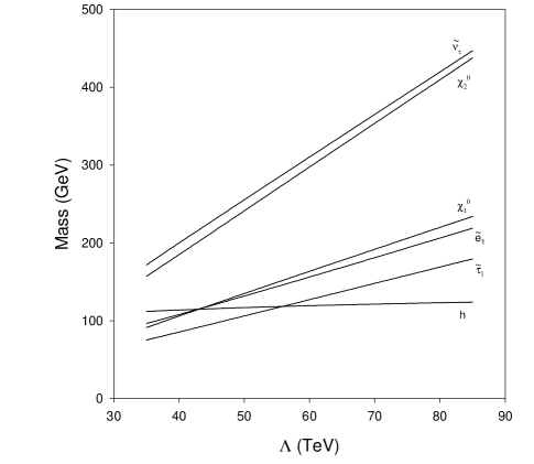
Figure 14: Masses of the particles of interest for the input parameters $tan\beta=15$, $M/\Lambda$ = 3, $n=2$, $f_{3}=0.5$, $f_{2}=0.05$, $f_{1}=0.05$ and $M_{\tilde{\Delta}}(M)=90$ GeV.

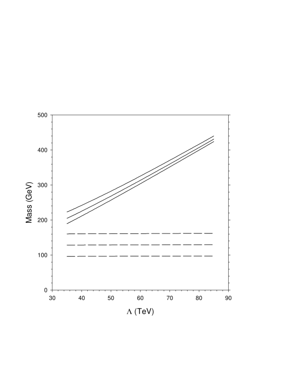
Figure 15: The dashed lines represent the deltino, while the solid lines represent the delta boson. From bottom to top, the lines in each set are for a messenger scale deltino mass of 90, 120 and 150 GeV.

In addition to these usual SUSY production mechanisms of the MSSM, we also have deltino pair ($\tilde{\Delta}^{c++}\tilde{\Delta}^{c--}$) production. This proceeds through s-channel $Z$ and $\gamma$ exchange. Given that the $\tilde{\Delta}^{c\pm\pm}$ can be relatively light, it can be a very important SUSY production mode. In fact, it frequently is the dominant mode. The masses of some of the particles of interest are given in Fig. 14 and Fig. 15. In Fig. 14 we take $M_{\tilde{\Delta}}(M)=90$ GeV (97 GeV at the weak scale), but the masses of the gauginos and sleptons (with the exception of the stau) do not vary much with the messenger scale deltino mass (M is the scale at which the soft breaking masses are introduced in the observable sector) . Fig. 15 gives the masses of the delta boson and the deltino. The deltino mass is not very sensitive to the value of $\Lambda$, while the delta boson mass is highly dependent on $\Lambda$ due to the contributions from the messenger scale loops.

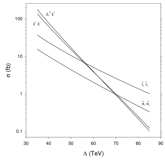
Figure 16: Cross sections for the standard SUSY production modes for $M_{\tilde{\Delta}}(M)=90$ GeV. (97 GeV at the weak scale.)

The cross sections for the more traditional SUSY production modes are given in Fig. 16. We also have deltino pair production; the cross sections for which are tabulated in Table 5. Since the deltino mass does not vary much over the values of $\Lambda$ ($\Lambda$ is related to the SUSY breaking scale) considered, the cross section for deltino pair production does not vary much either. This cross section is high enough for all the deltino masses considered that deltino pair production is always an important SUSY production mode.

VIII.3 Tau Jet Analysis

We now give an account of the possible $\tau$-jet signatures for SUSY production at the Tevatron in the context of the left-right GMSB model.

This analysis is performed in the context of the Main Injector (MI) and TeV33 upgrades of the Tevatron collider. The center of mass energy is taken to be $\sqrt{s}=2$ TeV and the integrated luminosity is taken to be 2 fb^-1 for the MI upgrade and 30 fb^-1 for the TeV33 upgrade.

In performing this analysis, the cuts employed are that final state charged leptons must have $p_{T}>10$ GeV. Jets must have $E_{T}>10$ GeV and $|\eta|<2$. In addition, hadronic final states within a cone size of $\Delta R\equiv\sqrt{(\Delta\phi)^{2}+(\Delta\eta)^{2}}=0.4$ are merged to a single jet. Leptons within this cone radius of a jet are discounted. For a $\tau$-jet to be counted as such, it must have $|\eta|<1$. The most energetic $\tau$-jet is required to have $E_{T}>20$ GeV. In addition, a missing transverse energy cut of ${\hbox to0.0pt{/\hss}E}_{T}>30$ GeV is imposed.

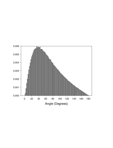
Figure 17: Angular distribution between the two most energetic $\tau$-jets for deltino pair production at the Tevatron. The deltino mass is about $97\hbox{\rm\,GeV}$. This plots gives the distribution when the $\tau$-jets come from same sign $\tau$ leptons.

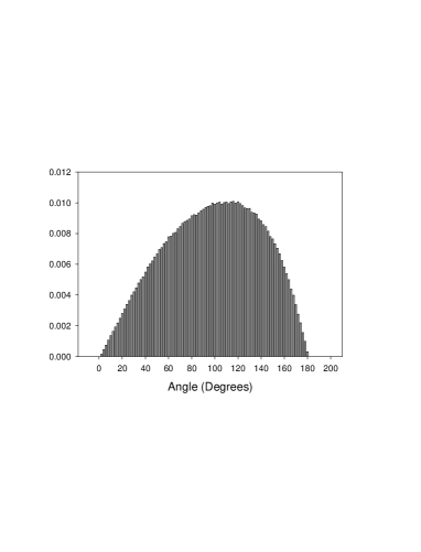
Figure 18: Angular distribution between the two most energetic $\tau$-jets for deltino pair production at the Tevatron. The deltino mass is about $97\hbox{\rm\,GeV}$. This plots gives the distribution when the $\tau$-jets come from opposite sign $\tau$ leptons.

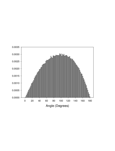
Figure 19: Angular distribution between the two most energetic $\tau$-jets for EW gaugino production at the Tevatron. The $\chi_{2}^{0}$ mass is 100 GeV. This plot gives the distribution when the $\tau$-jets come from same sign $\tau$ leptons.

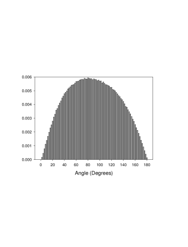
Figure 20: Angular distribution between the two most energetic $\tau$-jets for EW gaugino production at the Tevatron. The $\chi_{2}^{0}$ mass is 100 GeV. This plot gives the distribution when the $\tau$-jets come from opposite sign $\tau$ leptons.

In Table 6 we give the inclusive $\tau$-jet production cross sections for a messenger scale deltino mass of 90 GeV, respectively. We include only up to four $\tau$-jets as the cross sections for more than four $\tau$-jets are small. We see that before cuts the production of two and three $\tau$-jets are dominant, but the four $\tau$-jet cross section is also significant at slightly over 100 fb. After the cuts are applied, however, the situation changes substantially. The one $\tau$-jet mode is now dominant, but the cross section for two $\tau$-jets is not far below and the three $\tau$-jets cross section is not insignificant. For $\Lambda=35$ TeV the cross section for inclusive production of three $\tau$-jets is 32.3 fb. For an integrated luminosity of 2 fb^-1 (the approximate initial value at Run II), this corresponds to about 65 events. For 30 fb^-1, the number of observable events is $\sim 970$.

In comparison to the GMSB model with the MSSM symmetry, the two $\tau$-jets and the three $\tau$-jets cross sections are considerably higher in this model. In the GMSB model with MSSM symmetry, the two $\tau$-jets cross section can be seen at RUN II, but not the three $\tau$ jets mdn .

VIII.4 Angular Distributions

The excess of $\tau$-jets expected in this model does not constitute an unequivocal signal for this model. $\tau$-jets are part of the signatures for other models including the minimal GMSB model when the lighter stau is the NLSP. The question then arises as to whether there is any way to distinguish this model from the minimal GMSB model. A possible distinguishing characteristic is the distribution in angle between the two highest $E_{T}$ $\tau$-jets when they come from same sign $\tau$-jets.

Consider deltino pair production. The deltino tends to decay to like sign $\tau$ leptons. This occurs directly when the deltino is the NLSP and so decays via the three-body decay $\tilde{\Delta}^{\pm\pm}\rightarrow\tau^{\pm}\tau^{\pm}\tilde{G}$. When the two-body decay of the deltino $\tilde{\Delta}^{\pm\pm}\rightarrow\tilde{\tau}^{\pm}_{1}\tau^{\pm}$ occurs, then the second like sign $\tau$ lepton comes from the subsequent decay of the stau. In the rest frame of the deltino, the $\tau$ leptons are widely distributed. In the lab frame, however, the deltinos are quite energetic and have a large velocity, especially if their masses are small. As a consequence of this, the decay products of the deltino tend to be collimated in the direction in which the deltino was moving. Thus when the two most energetic $\tau$-jets have the same sign in deltino pair production, the angle between them tends to be smaller than when the two most energetic $\tau$-jets have opposite sign charges.

Fig. 17 gives the distribution in angle between the two most energetic $\tau$-jets for deltino pair production. This example is for a weak scale deltino mass of about 97 GeV. We can see that the distribution in angle for like sign $\tau$-jets, which is given in Fig. 17(a), peaks at about $40^{\circ}$. Fig. 17(b) gives the distribution in angle between the two most energetic $\tau$-jets when they come from opposite sign $\tau$ leptons. In stark contrast to the previous case, here the peak occurs at $110^{\circ}$.

The situation changes as the deltino mass gets larger. This is in part due to the fact that the deltino pair production cross section gets smaller and so production of charginos and neutralinos can have a larger impact on the distributions. In addition, a larger deltino mass means the deltinos will typically be moving slower.

Fig. 19 shows the angular distributions for combined $\chi_{2}^{0}\,\chi_{1}^{\pm}$ and $\chi_{1}^{+}\chi_{1}^{-}$ production for the weak scale $\chi_{2}^{0}$ mass is $\sim 100$ GeV. The distribution for same sign $\tau$-jets is given in Fig 5(a). We see that the peak occurs at about $110^{\circ}$. In $\chi_{2}^{0}\,\chi_{1}^{\pm}$ production, one of the same sign $\tau$-jets generally comes from the chargino and the other from the neutralino. We now consider the angular distribution for opposite sign $\tau$-jets which are given in Fig. 5(b). In $\chi_{2}^{0}\,\chi_{1}^{\pm}$ production, opposite sign $\tau$-jets frequently come from the neutralino, while in $\chi_{1}^{+}\chi_{1}^{-}$ production one of the $\tau$-jets comes from one of the charginos and the other $\tau$-jet comes from the other chargino. Since there is a strong possibility that the opposite sign $\tau$-jets come from the same particle ($\chi_{2}^{0}$), the distribution should peak at a lower angle than for same sign $\tau$-jets. We see from the figure that the peak occurs at about $85^{\circ}$. This feature does not change with the increase in the gaugino mass.

VIII.5 Conclusion

In conclusion, we have found that the doubly charged Higgs bosons of LR models can be potentially observable at Run II of the Tevatron through the production of $\tau$-jets. In a GMSB type theory, SUSYLR models typically produce large numbers of two and three $\tau$-jet final states. This large $\tau$-jet signal is also due in large part to pair production of the doubly charged Higgsino. It is also due to the relatively low mass of the lighter stau (which is frequently the NLSP) in these models, which is due to the additional coupling $f$. We have also shown that the distribution in angle between the two highest $E_{T}$ $\tau$-jets is different from other models which do not have this doubly charged Higgsino.

Table 5: Cross sections (in fb) for deltino pair production for various values of $\Lambda$. The other parameters used are $tan\beta=15$, $n=2$ and $M/\Lambda$ = 3.

$M_{\tilde{\Delta}}(M)$	$\Lambda=35$ TeV	$\Lambda=60$ TeV	$\Lambda=85$ TeV
90 GeV	643.0	629.9	621.5
120 GeV	228.2	222.9	219.6
150 GeV	91.6	89.2	87.7

Table 6: Inclusive $\tau$-jet for a messenger scale deltino mass of 90 GeV

$\Lambda$ (TeV)	35	40	50	60	70	80	85
	$\sigma\cdot{\rm BR}$ (fb)
1 $\tau$-jet: before cuts	198.6	132.9	73.11	71.64	70.86	70.34	70.14
after cuts	168.7	156.2	97.49	91.90	90.15	89.33	89.05
2 $\tau$-jets: before cuts	362.6	277.3	203.6	196.7	196.3	194.8	194.2
after cuts	124.6	93.11	89.59	82.91	80.59	79.63	79.33
3 $\tau$-jets: before cuts	306.0	273.5	253.6	244.7	240.9	238.8	238.0
after cuts	32.31	17.75	32.45	29.02	27.53	26.88	26.73
4 $\tau$-jets: before cuts	119.4	116.9	126.42	116.5	113.1	111.6	111.1
after cuts	3.21	1.18	5.26	4.28	3.67	3.45	3.39

IX Indirect Signals for Extra Dimensions

J.L. Hewett

One manifestation of theories of low scale quantum gravity is the existence of a Kaluza Klein (KK) tower of massive gravitons which can interact with the SM fields on the wall. In this section we examine the indirect effects of these massive gravitons being exchanged in Drell-Yan production. We consider a novel feature of this theory, namely, the contribution of gluon-gluon initiated processes to lepton pair production.

The effective theory below the effective Planck scale in the bulk, $M_{eff}$, consists of the SM fields on the wall and gravity which propagates in the full $4+n$ bulk. The interactions of these fields are given by

$$\int d^{4+n}x\,T^{\widehat{\mu}\widehat{\nu}}{h_{\widehat{\mu}\widehat{\nu}}(x^{\mu},x^{a})\over M_{eff}^{n/2+1}}\,,$$ (22)

where $T^{\widehat{\mu}\widehat{\nu}}$ is the symmetric, conserved stress-energy tensor in the bulk and $h_{\widehat{\mu}\widehat{\nu}}$ is the graviton field-strength tensor, which can be decomposed into spin-2, 1, and 0 fields. Here the indices $\widehat{\mu}$ extend over the full $4+n$ dimensions, $\mu$ over the $3+1$ dimensions on the wall, and $a$ over the $n$ bulk dimensions. The interactions with the SM matter fields are obtained by decomposing the above into the 4-dimensional states. The bulk fields $h_{\widehat{\mu}\widehat{\nu}}$ appear as Kaluza-Klein towers in the 4-dimensional space arising from a Fourier analysis over the cyclic boundary conditions of the compactified dimensions. Performing this decomposition, we immediately see that $T_{\mu a}=0$ and hence the spin-1 KK states don’t interact with the wall fields. The scalar, or dilaton, states couple proportionally to the trace of the stress-energy tensor. For interactions with fermions, this trace is linear in the fermion mass, while for gauge bosons it is quadratic in the boson mass. Hence, the dilaton does not contribute to the processes under consideration here.

We thus only have to consider the interactions of the KK spin-2 gravitons with the SM fields. All the gravitons in the KK tower, including the massless state, couple in an identical manner. Hence we may use the couplings to matter as obtained in the case of linearized general relativitygr . In this linearized theory, the matrix element for $q\bar{q}\rightarrow\ell^{+}\ell^{-}$ generalized for the case of $n$ massive graviton exchanges can be written as

$${\cal M}={1\over M_{Pl}^{2}}\sum_{n}{T^{e}_{\mu\nu}P^{\mu\nu\lambda\sigma}T^{f}_{\lambda\sigma}\over s-m^{2}_{gr}[n]}\,,$$ (23)

where the sum extends over the KK modes. $P_{\mu\nu\lambda\sigma}$ represents the polarization sum of the product of two graviton fields and is given in gr . The terms in the polarization sum that are quadratic and quartic in the transferred momentum do not contribute to the above matrix element since $T_{\mu\nu}$ is conserved. Likewise, the terms which go as $\eta_{\mu\nu}\eta_{\lambda\sigma}$ lead to terms proportional to $T_{\mu}^{e\mu}T_{\lambda}^{f\lambda}$ which vanish in the limit of zero electron mass. The remaining terms are $P_{\mu\nu\lambda\sigma}={1\over 2}[\eta_{\mu\lambda}\eta_{\nu\sigma}+\eta_{\mu\sigma}\eta_{\nu\lambda}-\eta_{\mu\nu}\eta_{\lambda\sigma}]$ and are exactly those present in the massless graviton case; they are thus universally applicable to all of the states in the KK tower. Since the spacing of the KK states is given by $\sim 1/r$, the sum over the states in (23) above can be approximated by an integral which is log divergent for $n=2$ and power divergent for $n>2$. A cut-off must then be applied to regulate these ultraviolet divergences, and is generally taken to be the scale of the new physics. For $n>2$ it can be shownsumm that the dominant contribution to this integral is of order $\sim M^{2}_{Pl}/M_{s}^{4}$, where we have taken the cut-off to be the string scale, while for $n=2$ this result is multiplied by a factor of order $\log(M_{s}^{2}/E^{2})$, where $E$ is the center-of-mass energy of the process under consideration. The exact computation of this integral can only be performed with some knowledge of the full underlying theory. Combining these results yields the matrix element

$${\cal M} = {\lambda\over M_{s}^{4}}\left\{\bar{q}(p_{1})\gamma_{\mu}q(p_{2})\bar{\ell}(p_{3})\gamma^{\mu}\ell(p_{4})(p_{2}-p_{1})\cdot(p_{4}-p_{3})\right.$$

$$\left.\bar{q}(p_{1})\gamma_{\mu}q(p_{2})\bar{\ell}(p_{3})\gamma_{\nu}\ell(p_{4})(p_{2}-p_{1})^{\nu}(p_{4}-p_{3})^{\mu}\right\}\,.$$

Here, the momentum flow is defined with $p_{1,2}$ into the vertex and $p_{3,4}$ outgoing. Note that graviton exchange is $C$ and $P$ conserving, and is independent of the flavor of the final state. The coefficient $\lambda$ is of ${\cal O}(1)$ and cannot be explicitly calculated without knowledge of the full quantum gravity theory. It is dependent on the number of extra dimensions, how they are compactified, and is in principle a power series in $s/M_{s}^{2}$. However, we neglect this possible energy dependence in $\lambda$ and note that the limits obtained here, which go as $|\lambda|^{1/4}$, are only very weakly dependent on its precise value and hence on the specific model realization. In principle the sign of $\lambda$ is undetermined and we examine the constraints that can be placed on $M_{s}$ with either choice of signs.

The angular distribution for $q\bar{q}\rightarrow\ell^{+}\ell^{-}$ with massless leptons is then calculated to be

$${d\sigma\over dz} = N_{c}{\pi\alpha^{2}\over 2s}\left\{P_{ij}\left[A^{q}_{ij}A^{\ell}_{ij}(1+z^{2})+2B^{q}_{ij}B^{\ell}_{ij}z\right]\right.$$

$$-{\lambda s^{2}\over 2\pi\alpha M_{s}^{4}}P_{i}\left[2z^{3}v^{q}_{i}v^{\ell}_{i}-(1-3z^{2})a^{q}_{i}a^{\ell}_{i}\right]$$

$$\left.+{\lambda^{2}s^{4}\over 16\pi^{2}\alpha^{2}M_{s}^{8}}\left[1-3z^{2}+4z^{4}\right]\right\}\,,$$

where the indices $i,j$ are summed over $\gamma$ and $Z$ exchange, $z=\cos\theta$, $P_{ij}$ and $P_{i}$ are the usual propagator factors (defined in e.g., leptos ), $A^{f}_{ij}=(v_{i}^{f}v_{j}^{f}+a_{i}^{f}a_{j}^{f})$ , and $B^{f}_{ij}=(v_{i}^{f}a_{j}^{f}+v_{j}^{f}a_{i}^{f})$. Note that the total cross section from $q\bar{q}$ annihilation is unaltered by graviton exchanges, independently of fermion flavor up to terms of order $s^{4}/M_{s}^{8}$, and hence the angular distributions will be most sensitive to these new exchanges.

In addition to the $q\bar{q}$ channel, gravitons can also mediate gluon-gluon contributions to lepton pair production via $s$-channel exchange, as noted above. Such gluon initiated processes are a remarkable consequence of this theory and have the potential to modify the Drell-Yan spectrum in a unique manner. Following an analogous procedure as outlined above for the four-fermion case, the matrix element for $gg\rightarrow\ell^{+}\ell^{-}$ via graviton exchanges is found to be

$${\cal M} = {-\lambda\over 4M_{s}^{4}}\bar{\ell}(p^{\prime})[(p^{\prime}-p)_{\mu}\gamma_{\nu}+(p^{\prime}-p)_{\nu}\gamma_{\mu}]\ell(p)\left\{k^{\prime}_{\alpha}(k_{\mu}\eta_{\beta\nu}+k_{\nu}\eta_{\beta\mu})+k_{\beta}(k^{\prime}_{\mu}\eta_{\alpha\nu}+k^{\prime}_{\nu}\eta_{\alpha\mu})\right.$$

$$\left.-\eta_{\alpha\beta}(k^{\prime}_{\mu}k_{\nu}+k_{\mu}k^{\prime}_{\nu})+\eta_{\mu\nu}(k^{\prime}\cdot k\eta_{\alpha\beta}-k_{\beta}k^{\prime}_{\alpha})-k\cdot k^{\prime}(\eta_{\mu\alpha}\eta_{\nu\beta}+\eta_{\mu\beta}\eta_{\nu\alpha}\right\}\epsilon^{\beta}_{g}(k^{\prime})\epsilon^{\alpha}_{g}(k)\,,$$

where the momentum flow is defined with both $k\,,k^{\prime}$ flowing into the vertex and $p\,,p^{\prime}$ being outgoing and $\epsilon$ represents the gluon polarization vector. Because the graviton couplings and the summation over the KK tower of states for $2\rightarrow 2$ processes are universal, $\lambda$ is the same ${\cal O}(1)$ coefficient as in Eq. (IX). This matrix element yields the $gg\rightarrow\ell^{+}\ell^{-}$ differential cross section for massless leptons

$${d\sigma\over dz}={\lambda^{2}\widehat{s}^{3}\over 64\pi M_{s}^{8}}(1-z^{2})(1+z^{2})\,,$$ (27)

which has a remarkably simple form. While the overall numerical coefficient appears to be very small, it must be compared to $\sim\alpha^{2}$ which appears in the usual contributions to Drell-Yan production. In addition, the large parton luminosity for gluons at higher energy colliders may also compensate for the small numerical factor. Since this cross section is also even in $\cos\theta$, the gluon-gluon contributions will only affect the total cross section and not the forward-backward asymmetry. Also note that the ambiguity in the sign of $\lambda$ does not affect the gluon-gluon contributions as they do not interfere with the $q\bar{q}$ initiated process.

The bin integrated lepton pair invariant mass distribution and forward-backward asymmetry $A_{FB}$ is presented in Fig. 21. In each case the solid histogram represents the SM expectations, and the ‘data’ points include the graviton exchanges with the error bars representing the statistics in each bin. The rapidity cuts, parton density parameterizations, and assumed integrated luminosity are as labeled, and we have summed over electron and muon final states. Here we present the sample case of $M_{s}=800$ GeV and the sign ambiguity in $\lambda$ is visible in the forward-backward asymmetry. Since the graviton exchanges only affect the invariant mass distribution at order $\lambda^{2}/M_{s}^{8}$, we expect only minor modifications to this spectrum and we see that this holds true. For higher energy colliders which have a larger gluon parton luminosity, such as the LHC, large string scales do have a sizable effect on the $M_{\ell\ell}$ spectrumjlh . However, the deviations in $A_{FB}$, are more pronounced at the Tevatron, where even the two cases $\lambda=\pm 1$ are statistically distinguishable from each other for this sample case. The resulting 95% C.L. search reach are given in Fig. 23. We also find that present Tevatron data from Run I with 110 ${\rm pb}^{-1}$  of integrated luminosity excludes a string scale up to 980 (920) GeV at 95% C.L. for $\lambda=-1(+1)$.

Figure 21: Bin integrated lepton pair invariant mass distribution for Drell-Yan production at the Main Injector. The SM is represented by the solid histogram. The data points represent graviton exchanges with $M_{s}=800$ GeV and $\lambda=+1$ or $-1$.

Figure 22: Bin integrated lepton pair forward-backward asymmetry for Drell-Yan production at the Main Injector. The SM is represented by the solid histogram. The data points represent graviton exchanges with $M_{s}=800$ GeV and $\lambda=+1$ or $-1$.

Figure 23: 95% C.L. search reach for the string scale as a function of integrated luminosity at the Tevatron with the sign of $\lambda$ as labeled.

X Higgs Bounds in Three and Four Generation Scenarios

D. Dooling, K. Kang and S.K. Kang

X.1 Introduction

The search for the Higgs boson being one of the major tasks along with that for supersymmetric sparticle and fourth generation fermions at future accelerators such as LEP200 and LHC makes it a theoretical priority to examine the bounds on the Higgs boson mass in the SM and its supersymmetric extension and to look for any distinctive features. The actual measurement of the Higgs boson mass could serve to exclude or at least to distinguish between the SM(3,4) and the MSSM(3,4) models for electroweak symmetry breaking. Recently, bounds on the lightest Higgs boson mass were calculated in 1 ; 2 ; 3 ; 4 ; 5 ; 6 ; 7 ; 8 ; 9 . It was found that for a measured $M_{H}$ lying in a certain mass range, both the SM vacuum stability lower bound and the MSSM upper bound are violated, thus shaking our confidence in these theories just as the final member of the mass spectrum is observed. One method of curing this apparent illness is to take a leap of faith by adding another fermion generation, to fortify these theories with another representation of the gauge group. This additional matter content, for certain ranges of its mass values, has the desired effect of raising the MSSM3 upper bound above that of the SM lower bound and avoids the necessity of being forced to introduce completely new physics.

In this work, we use the latest LEP Electroweak Working Group data as well as the most recent experimental lower limits on the masses of fourth generation fermions to see how the Higgs boson mass bounds are affected. With only the standard three generations, a violation of both the SM and the MSSM bounds occurs for a broad range of $M_{H}$ values, signalling the need for an additional generation. Our presentation is organized as follows. We first present a summary of our one-loop effective potential (EP) improved by the two-loop renormalization group equations (RGE) analysis. An expression for the Higgs boson mass is derived up to the next-to-leading logarithm order. Bounds on $M_{H}$ are obtained by imposing different boundary conditions on the Higgs self-coupling $\lambda$. Finally, we present our results and also obtain information on the possible mass range of the fourth generation leptons, $M_{L}$.

X.2 Effective Potential Approach

As shown in 10 , in order to calculate the Higgs boson mass up to the next-to-leading logarithm approximation, we must consider the one-loop EP improved by two-loop RGE for the $\beta$ and $\gamma$ functions of the running coupling constants, masses and the $\phi$ field for the Higgs boson 11 .

The two-loop RGE improved one loop EP of the SM4 is given by

$$V_{1}=V_{(0)}+V_{(1)}$$ (28)

where

$$V_{(0)} = -\frac{1}{2}m^{2}(t)\phi_{c}^{2}(t)+\frac{1}{24}\lambda(t)\phi_{c}^{4}(t)$$ (29)

$$V_{(1)} = \sum_{i=1}^{5}\left(-\frac{\kappa_{i}}{64\pi^{2}}\right)h_{i}^{4}(t)\phi_{c}^{4}(t)\left[{\rm ln}\,\frac{h_{i}^{2}(t)\zeta^{2}(t)}{2}-\frac{3}{2}\right]$$ (30)

Here $\phi_{c}$ is the classical field corresponding to the physical Higgs boson $\phi$, $i=(t,T,B,N,E)$ , $~{}\kappa_{i}=3$ for $i=(t,T,B)$ and $\kappa_{i}=1$ for $i=(N,E)$ and $h_{i}$ is the Yukawa coupling of the i^th fermion to the Higgs field. In addition,

$$\zeta(t) = \left(-\int_{0}^{t}\gamma_{\phi}(t^{\prime})dt^{\prime}\right)$$ (31)

$$\phi_{c}(t) = \phi_{c}\zeta(t)$$ (32)

and

$$\mu(t)=\mu\exp(t)$$ (33)

where $\mu$ is a fixed scale.

Starting with the above expression for the SM(3,4) EP, one may follow the analysis in 1 ; 4 and obtain the expression for the Higgs boson mass:

$$m_{\phi}^{2} = \frac{1}{3}\lambda v^{2}+\frac{\hbar v^{2}}{16\pi^{2}}\left\{\frac{\lambda^{2}}{3}+2\lambda(h_{t}^{2}+h_{T}^{2}+h_{B}^{2})+\frac{2\lambda}{3}(h_{E}^{2}+h_{N}^{2})\right.$$ (34)

$$-\frac{\lambda}{2}(3g_{2}^{2}+g_{1}^{2})+\frac{9}{8}g_{2}^{4}+\frac{3}{4}g_{1}^{2}g_{2}^{2}+\frac{3}{8}g_{1}^{4}$$

$$-6h_{t}^{4}{\rm ln}\,\frac{h_{t}^{2}\zeta^{2}}{2}-6h_{T}^{4}{\rm ln}\,\frac{h_{T}^{2}\zeta^{2}}{2}-6h_{B}^{4}{\rm ln}\,\frac{h_{B}^{2}\zeta^{2}}{2}$$

$$\left.-2h_{E}^{4}{\rm ln}\,\frac{h_{E}^{2}\zeta^{2}}{2}-2h_{N}^{4}{\rm ln}\,\frac{h_{N}^{2}\zeta^{2}}{2}\right\}+O(\hbar^{2})$$

where the three generation case is obtained by simply letting the fourth generation Yukawa couplings go to zero.

Following the method similar of Kodaira et al. 4 , we arrive at the appropriate energy scale at which to evaluate $\frac{\partial^{2}V}{\partial\phi_{c}(t)^{2}}$ by requiring $\frac{\partial V}{\partial\phi_{c}(t_{v})}=$ 0 at the scale $t_{v}$ where $\phi_{c}(t_{v})=v=(\sqrt{2}G_{F})^{-\frac{1}{2}}$ = 246 GeV. $t_{v}$ is found to satisfy:

$$t_{v}={\rm ln}\,\frac{v}{\mu}+\int_{0}^{t_{v}}\gamma_{\phi}(t^{\prime})dt^{\prime}.$$

We then evaluate the first and second derivatives of the EP at the scale $t_{v}$ where $\phi_{c}(t_{v})=v$. In the above relation satisfied by $t_{v}$, $\mu$ is a fixed, constant mass scale. In the MSSM theories, we will take $\mu$ to be $M_{susy}=1$ or 10 TeV, while the SM lower bounds will be derived after choosing $\mu=\Lambda=10^{19}$ GeV.

We define the running Higgs mass as:

$$m_{h}^{2}(t)=\frac{m_{h}^{2}(t_{v})\zeta^{2}(t_{v})}{\zeta^{2}(t)}.$$

The physical, pole masses are related to the running masses via the following equations:

$$M_{i}=\left[1+\beta_{i}\frac{4\alpha_{3}(M_{i})}{3\pi}\right]m_{i}(M_{i})$$

$$M_{H}^{2}=m_{h}^{2}(t)+Re\Pi(M_{H}^{2})-Re\Pi(0)$$

where $\beta_{i}$ = 0 for i = (N,E) and = 1 for i = (t,T,B). $\Pi(q^{2})$ is the renormalized electroweak self-energy of the Higgs boson.

The method of solving the RGE and the appropriate boundary conditions for the couplings is explained in 1 . In this update, we use $M_{Z}=91.1867$ GeV and $\alpha_{3}(M_{Z})=.119$.

X.3 Bounds on $M_{H}$

Let us first discuss the procedure for determining a lower bound on the Higgs boson mass in the SM 5 ; 12 Working with the two-loop RGE requires the imposition of one-loop boundary conditions on the running parameters. As pointed out by Casas et al. 5 ; 7 , the necessary condition for vacuum stability is derived from requiring that the effective coupling $\tilde{\lambda}(\mu)>$ 0 rather than $\lambda>0$ for $\mu(t)<\Lambda$, where $\Lambda$ is the cut-off beyond which the SM is no longer valid. The effective coupling $\tilde{\lambda}$ in the SM4 is defined as:

$$\tilde{\lambda}=\frac{\lambda}{3}-\frac{1}{16\pi^{2}}\left\{\sum_{i=1}^{5}2\kappa_{i}h_{i}^{4}\left[{\rm ln}\,\frac{h_{i}^{2}}{2}-1\right]\right\}$$

where the three generation case is simply the same as the above expression without the fourth generation Yukawa coupling contributions. Choosing $\Lambda=10^{19}$ GeV and $M_{top}=172$ GeV, we arrive at a vacuum stability lower bound on $M_{h}$ of $\sim$ 134 GeV for the SM with three generations. Allowing $M_{top}$ to be as large as 179 GeV increases the lower bound on $M_{H}$ to $\sim$ 150 GeV.

To compute the MSSM upper bound on $M_{H}$, we assume that all of the sparticles have masses $O(M_{susy})$ or greater and that of the two Higgs isodoublets of the MSSM, one linear combination is massive, also with a mass of $O(M_{susy})$ or greater, while the other linear combination, orthogonal to the first, has a mass of the order of weak-scale symmetry breaking. With these two assumptions, it is clear that below the supersymmetry breaking scale $M_{susy}$, the effective theory is the SM. This fact enables us to use the SM effective potential for the Higgs boson when we treat the lightest Higgs boson in the MSSM.

In the MSSM(3,4), the boundary condition for $\lambda$ at $M_{susy}$ is

$$\frac{\lambda}{3}(M_{susy})=\frac{1}{4}\left[g_{1}^{2}(M_{susy})+g_{2}^{2}(M_{susy})\right]\cos^{2}(2\beta)+\frac{\kappa_{i}h_{i}^{4}(M_{susy})}{16\pi^{2}}\left(2\frac{X_{i}}{M_{susy}^{2}}-\frac{X_{i}^{4}}{6M_{susy}^{4}}\right)$$

where $\kappa_{i}$ = 3 for $i=(t,T,B)$ and $\kappa_{i}$ = 1 for $i=(N,E)$ and $X_{i}$ is the supersymmetric mixing parameter for the ith fermion. Zero threshold corrections correspond to $X_{i}$ = 0. Maximum threshold corrections occur for $X_{i}=6M_{susy}^{2}$.

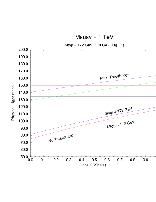
Figure 24: The lightest Higgs boson mass $M_{H}$ as a function of $\cos^{2}(2\beta)$. The bottom two curves correspond to MSSM upper bounds with no threshold corrections, for $M_{top}$ = 172 GeV and 179 GeV, respectively. The two upper curves correspond to MSSM upper bounds with maximum threshold corrections, for $M_{top}$ = 172 GeV and 179 GeV, respectively. The two horizontal lines are the $\cos^{2}(2\beta)$-independent SM3 vacuum stability bounds. The lower horizontal line corresponds to $M_{top}$ = 172 GeV, while the other horizontal line was computed with $M_{top}$ = 179 GeV.

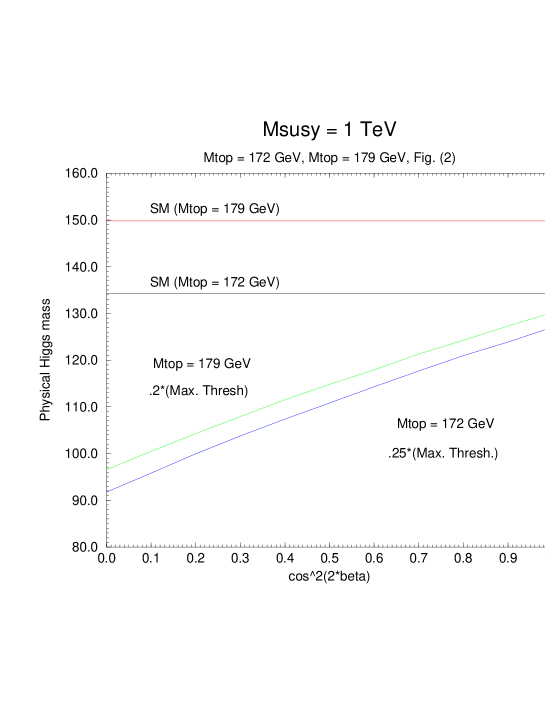
Figure 25: Same as Figure 1, but now the MSSM bounds correspond to the minimal threshold corrections consistent with the experimental lower limit on $M_{H}$.

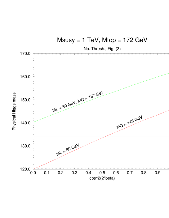
Figure 26: Plots of the physical Higgs boson mass as a function of $\cos^{2}(2\beta)$. The $\cos^{2}(2\beta)$-independent flat line is the MSSM3 vacuum stability lower bound for $M_{top}$ = 172 GeV. The lower curve is the MSSM4 upper bound for the same value of $M_{top}$, no threshold corrections and the indicated values for $M_{L}$ and $M_{Q}$. Similarly for the upper curve. Figure 4: Same as Figure 3, but with $M_{top}$ = 179 GeV.

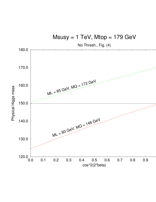
Figure 27: See caption of Fig. 26.

In Fig. (1) we present our numerical two-loop results for the lightest Higgs boson mass bounds in the SM and the MSSM3 as a function of the supersymmetric parameter $\cos^{2}(2\beta)$. The bottom two curves correspond to the MSSM3 upper bound for the two cases $M_{top}=172$ GeV and the slightly greater upper bound that results when $M_{top}$ = 179 GeV and with no threshold corrections. When the case of maximum threshold corrections is considered, these two curves are translated upwards by $\sim$ 55 GeV - 60 GeV, illustrating the strong dependence of the upper bound on the precise value of the threshold corrections. Yet even with such a dramatic increase in the upper bounds with increasing threshold corrections, we observe that the SM lower bound exceeds the MSSM upper bound for $M_{top}=172$ GeV and $0<\cos^{2}(2\beta)<.2$ for all values of the threshold correction contribution. Similarly, for $M_{top}=179$ GeV, the troublesome situation is only exacerbated, as the SM lower bound exceeds the MSSM upper bound for $0<\cos^{2}(2\beta)<.38$ independent of the threshold corrections.

In Fig.(2) we present the problem more clearly. Taking into account the present experimental lower limit on $M_{H}$ of $\sim$ 90 GeV at 95$\%$ CL, we find the value of the threshold correction that gives a smallest upper bound consistent with the experimental lower limit. Clearly, for this phenomenologically determined lower limit of the threshold contributions, there is a large area in $M_{H}\times\cos^{2}(2\beta)$ space that is inconsistent with both the SM and the MSSM. For $M_{top}=172$ GeV, the region 92 GeV $<M_{H}<$ 134 GeV invalidates both theories independent of $\cos^{2}(2\beta)$, while for $M_{top}=179$ GeV, the range of mutual invalidation is 92 GeV $<M_{H}<$ 150 GeV.

X.4 Fourth Generation

To resolve the above conundrum, one would like to either raise the MSSM upper bounds, lower the SM lower bounds, or both. Adding more massive fermions to the theory only increases both bounds, so it is readily apparent that the way out of the area of inconsistency is to consider the MSSM4 and see if the additional matter of the MSSM4 results in MSSM4 upper bounds that exceed the SM3 lower bounds.

We now discuss restrictions on the possible fourth generation fermion masses 2 ; 13 ; 14 ; 15 . The close agreement between the direct measurements of the top quark at the Tevatron and its indirect determination from the global fits of precision electroweak data including radiative corrections within the framework of the SM imply that there is no significant violation of the isospin symmetry for the extra generation. Thus the masses of the fourth generation isopartners must be very close to degenerate 14 ; i.e.

$$\frac{\|M_{T}^{2}-M_{B}^{2}\|}{M_{Z}^{2}}\lesssim 1,\frac{\|M_{E}^{2}-M_{N}^{2}\|}{M_{Z}^{2}}\lesssim 1$$

Recently, the limit on the masses of the extra neutral and charged lepton masses, $M_{N}$ and $M_{E}$, has been improved by LEP1.5 to $M_{N}>59$ GeV and $M_{E}>62$ GeV. Also, CDF has yielded a lower bound on $M_{B}$ of $\sim$ 140 GeV.

In our previous work, we considered a completely degenerate fourth generation of fermions with mass $m_{4}$. We derived an upper bound on $m_{4}$ in the MSSM4 by demanding perturbative validity of all the couplings out to the GUT scale 16 . This constraint led to an upper bound on $m_{4}$ of $\sim$ 110 GeV. The above experimental lower limit on $M_{B}$ naturally forces us to now a consider a fourth generation where degeneracy only holds among the isodoublets separately. We therefore consider a fourth generation with masses $M_{L}$ and $M_{Q}$.

In Fig.(3), we present the SM lower bound, the MSSM4 upper bound with the fourth generation masses at their experimental lower limits and with fourth generation masses large enough to remove the problem area for all values of $\cos^{2}(2\beta)$. The MSSM bounds were calculated with no threshold corrections, and $M_{top}$ is fixed at 172 GeV. Fig.(4) shows the same information for $M_{top}$ = 179 GeV. The MSSM4 upper bounds are much more sensitive to $M_{Q}$ than they are to $M_{L}$. This qualitative behavior is readily understood from inspection of the equation for $m_{\phi}^{2}$. For this reason, it is necessary to increase $M_{Q}$ appropriately in order to generate a MSSM4 upper bound that is greater than the SM lower bound for all values of $\cos^{2}(2\beta)$. In fact, keeping $M_{Q}$ at 146 GeV and allowing $M_{L}$ to be 110 GeV does not resolve the problem. But increasing both $M_{Q}$ and $M_{L}$ as indicated in the figures does remove the problem. Because all of the bounds increase as $M_{L}$ and $M_{Q}$ increase, and because the upper bounds on $m_{4}$ from the previous work are saturated when the masses of the fourth generation reach some critical values from below, we can conclude that $M_{L}$ must still be $<110$ GeV. This conclusion follows because it is $h_{N}$ that violates perturbative validity, so in the non-degenerate case, it is $M_{L}$ that must still respect this upper bound if gauge coupling unification is still to be achieved in the MSSM4.

X.5 Concluding remarks

In conclusion, we have studied the upper bounds on the lightest Higgs boson mass $M_{H}$ in the MSSM with four generations by solving the two-loop RGE’s and using the one-loop EP. We have considered a fourth generation of quarks and leptons with degenerate masses $M_{Q}$ and $M_{L}$. For certain values of $M_{Q}$ and $M_{L}$, the area of mutual inconsistency between the SM and MSSM3 Higgs mass bounds is found to be consistent with the MSSM4 upper bounds.

XI Fourth Family Status and Prospects

D. McKay

XI.1 The Bottom Line

In light of the general expectation from SUSY considerations and from precision electroweak fits that the lightest Higgs is light, I believe that the inclusion of the essential Higgs FCNC channel in the simulation of the various decay channels of $b^{\prime}$ is the the fourth family project that deserves a strong effort among the BTMSSM searches. Analysis of the $b^{\prime}\rightarrow b+Z$ mode is well advanced at both CDF and D0. The inclusion of the Higgs mode, with the subsequent $H\rightarrow b+\overline{b}$ decay, will remove the last loophole in the $b^{\prime}$ search up to the top mass. A good reason for stressing this issue is that it ties in directly to the crucial Higgs search mission at Run II, which makes the $b^{\prime}$ search more subtle and more interesting.

A small but important project is the re-fitting of electroweak parameters to include relatively light new physics (50-150 GeV) effects. A preliminary look is shown in the “mass bounds” graph in Section 3.

More detail on these points is given in Sec. 3 below.

XI.2 Words of Motivation

1) There is no theoretical reason against having a fourth family. Since there is no solid theoretical understanding of the family pattern, there is motivation to simply look to see if a new one shows up. Unless stated otherwise, fourth family means a family with a lepton doublet with mass greater than $m_{Z}$/2 but with an otherwise sequential, chiral set of leptons $(\nu^{\prime},\tau^{\prime})$ and quarks $(t^{\prime},b^{\prime})$. (It is assumed in all of the discussion that $V_{b^{\prime}t^{\prime}}\gg V_{b^{\prime}t}\simeq V_{t^{\prime}b}\gg V_{b^{\prime}c}$

2) Though it is not in the vein of the fourth family as just defined, the proposal by Frampton and collaborators to solve the strong CP problem calls for heavy vector-like fermion states, and the search strategies are largely the same as for chiral lepton and quark states. ( see Frampton and Kephart, PRL 66, 166; Frampton and Ng, PRD 43, 3034).

3) In a four family extension of the standard model, Hung has recently argued that unification of the gauge couplings can be obtained at a high enough scale to avoid proton decay. The scale for the fourth family can be higher than in the MSSM, but it is still constrained to rather low values - lepton masses below $m_{Z}$ and quark masses at around $m_{t}$ - by the requirement that all couplings stay perturbative up to the unification scale. If this motivation applies to SUSY, it applies to this four family SM. The hierarchy problem is left unsolved, of course. ( P.Q. Hung, PRL 80, 3000 (1998); see also P. Frampton and P.Q. Hung, Phys. Rev. D 58, 057704 (1998) for phenomenology of quasi-stable quarks in the $\sim m_{t}$ range that could have escaped detection in the CDF and D0 analysis to date. For a study of four family consequences in the MSSM with SUGRA boundary conditions, see J. Gunion, D. McKay and H. Pois, PRD 53, 1616,(1996) ).

4) For those with a taste for dynamical breaking of electroweak symmetry, new heavy quark flavors in a fourth family may have some appeal, since the heavy quark condensate mechanism for EW breaking may have a chance if there are extra, heavy quarks in the range 150-230 GeV to help top do the job. (see for example Hung and Isidori, P.L. B402, 122).

5) Tying in directly with the Higgs boson search and BTMSSM theme of this workshop, D. Dooling, K. Kang and S.-K. Kang (hep-ph/9710258, to be published, and contribution to this workshop) have argued that the lower mass bound on the SM Higgs boson and the upper limit on the lightest Higgs in the MSSM are relaxed in four family extensions of these models. This consideration is especially timely as the limit on the SM Higgs mass has recently been pushed up to nearly 100 GeV at LEP II.

XI.3 Experimental Facts that tightly constrain a sequential Fourth Family

1) The S parameter in precision electroweak analysis is now $S=-0.16\pm 0.14(-0.10)$ as listed by the PDG ’98 discussion of ”Electroweak model and constraints on new physics”(European Physical Journal C 3,1 (1998)). A new, heavy (several times $M_{Z}$) degenerate, chiral family adds $2/3\pi$ to S and this excludes an extra, heavy family of fermions at the 99.2% C.L. when S is allowed to be arbitrary and fixed by the values of the EW parameters fit at the Z (primarily). Requiring S to be positive with a given Higgs mass relaxes this bound somewhat. If some of the masses of the family members are in the neighborhood of $m_{Z}$, then the theoretical value of S is less than $2/3\pi$, and a more general analysis of the data is called for (I. Maksymyk, C.P. Burgess and D. London, Phys. Rev. D 50, 529 (1994)). In the “mass bounds” figure, the S parameter bound excludes all of the region to the right of the curve in this plot at the 95% C.L. $m_{Q}/m_{Z}$ is plotted on the y axis vs $m_{L}/m_{Z}$ on the x axis. The Q and L designate mass degenerate quark and lepton doublets, respectively. ($S\leq 0.15$) is the constraint. Clearly the (chiral) lepton doublet must be very light to satisfy this requirement. The constraint is insensitive to the quark masses because they nearly, but not quite, saturate the bound by themselves for large quark mass values, so they have little effect when $m_{Q}/m_{Z}>1.5$.

Figure 28: The region below the $b^{\prime}->b+Z$ curve, to the right of the S-parameter curve, and above the Landau pole curve are excluded. This leaves the small rectangular allowed region at the far left and center of the figure.

A completely consistent re-fit to the data with relatively light, fourth family doublets needs to be done and is in the works.

2) The direct searches for $b^{\prime}\rightarrow b+V(\gamma,Z,g)$ have severely narrowed the options below $M_{b^{\prime}}=140GeV$. The D0 Collaboration ( PRL 78, 3817 (1997)) reported the $b^{\prime}\rightarrow b+\gamma$ bound of $m_{b^{\prime}}<95GeV$ at 95% C.L. 95 GeV is the limit for this mode, since the larger b+Z mode sets in here. Results of a study of the $b^{\prime}\rightarrow b+Z$ mode were reported by Joao Guimaraes da Costa of CDF at the April, ’98 AAPT/APS meeting (see also the contribution by Dave Stuart to this workshop). A limit $m_{b^{\prime}}>140GeV$ at 95% C.L. is achieved, assuming that $\Gamma(b^{\prime}\rightarrow b+Z)=100\%$. This bound is shown by the horizontal line in the “mass bounds” figure. A slip knot in this noose tightening around b’ could be the $b^{\prime}\rightarrow b+H$ mode, which is likely to be as large as or larger than the b+Z mode. This would seriously degrade the $b^{\prime}$ mass bounds quoted unless the Higgs final state were included in the tagged sample with favorable efficiencies. Failing this, roughly speaking, when the b+Higgs decay mode is accessible to $b^{\prime}$, the $b+\gamma$ quoted number of expected events would be halved and the expected b+Z events would be quartered. But in fact, as argued by Guimaraes da Costa (private communication), if the Higgs + b final state is present, it will be included in the sample as long as the b + Z branching fraction is not zero so that the lepton tagging of the Z is operative. Moreover the efficiency for tagging the b’s from Higgs decay is good enough that the factor 4 decrease in events from the competing channel is compensated. The bottom line is that if $m_{Z}\sim m_{H}$, the bound $m_{b^{\prime}}<140GeV$ is still likely to obtain. The b+Z and b+H decay rates are roughly proportional to $m_{t}^{2}-m_{t^{\prime}}^{2}$, so their ratio is insensitive to $m_{t^{\prime}}$, but when $m_{t^{\prime}}\sim m_{t}$ with $m_{b^{\prime}}<m_{t^{\prime}}$, then $b^{\prime}\rightarrow c+W$ or $b^{\prime}\rightarrow c+W^{*}$ becomes potentially important. These issues are thoroughly considered in, for example, W-S. Hou and R.G. Stuart, Phys. Rev. D 43, 3669 (1991). What is new is the near consensus from SUSY and precision electroweak fits that the lightest Higgs mass is between $m_{Z}$ and $m_{t}$. I believe that the simulation of competing effects of the various decay channels of $b^{\prime}$ and the onset of the $t^{\prime}$ threshold and decays, with inclusion of the essential Higgs FCNC channel, is the project that deserves a strong effort in Run II. The reason for stressing this issue is that it ties in directly to the crucial Higgs search mission at Run II. A search for the FCNC decay modes of $b^{\prime}$ or $t^{\prime}$ must include the Higgs effects.

CDF has analyzed its data for the presence of long-lived charged 1/3 $(b^{\prime})$ and 2/3 $(t^{\prime})$ quarks and has reported mass limits of 195 GeV and 220 GeV at 95% C.L. This pretty analysis closes the door on the possibility that top search signatures missed stable $(\gamma\tau>10^{-8}s)$ $b^{\prime}$ or $t^{\prime}$ ( Dave Stuart, contribution to this workshop).

3) Searches for N and L leptons by the LEPII detector groups limit masses of stable charged leptons to be above 90 GeV at 95% C.L.(eg. OPAL Collaboration, Phys.Lett.B, 433, 195 (1998). Analysis of LEPII data also shows that unstable lepton doublets can escape detection only if N and L are degenerate at the level of a GeV or so, with the neutral one lighter and stable enough to exit the detector. (see S. Thomas and J. Wells, hep-ph/9804359 for a technique to detect such states. The motivation is that vector-like doublets with radiative splitting on the order of several hundreds of MeV are typical in a variety of motivated extensions to SM, but the analysis applies equally well to “unmotivated” doublets).

XI.4 Considerations on Unification and Perturbation Theory, SUSY Breaking and Other Theory Prejudices

As mentioned above, requiring that perturbation theory remain valid as Yukawa and gauge coupling constants are run to the grand unification scale tightly constrains new family masses. The Yukawa couplings blow up (Landau poles) sooner or later as they are run to higher and higher mass scales. The bigger they start (big masses at the weak scale), the faster they take off. Because of the many superpartners, this effect is exaggerated in the MSSM compared to the SM. Even the latter suffers rapid blow up when fourth family quark masses exceed 150 GeV or so (a recent study is reported in Yu. F. Pirogov and O.V. Zenin, hep-ph/9808396). In the context of a fourth family extension of the MSSM, the constraint is severe indeed. Setting the top mass in the range 170- 175 GeV and requiring that all couplings run to the GUT scale at a few times $10^{16}$ GeV, one finds that $m_{b^{\prime}}<100GeV$ and $m_{t^{\prime}}<120GeV$. Unless the lightest MSSM Higgs boson is at the Z mass or less, the D0 and CDF searches eliminate a $b^{\prime}$ with a mass this low. In the framework of gravity mediated SUSY breaking and the SUGRA boundary conditions, giving up perturbative unification means giving up the predictions of the SUSY mass spectrum at low energy, since the mass parameters are all specified at the GUT scale. This is a punishing penalty to pay! In gauge mediated SUSY breaking, however, the mass parameters are set at the messenger scale - roughly 100 TeV. Within this picture of SUSY breaking, one may require perturbative running of the coupling constants ${onlytothemessengerscale}$, still retain predictive power over the SUSY mass spectrum, and buy a wider range of theoretically acceptable fourth family mass values. The result of a preliminary one-loop RG study is shown in the “Landau Pole Bound” curve on the “mass bounds” figure for the case $tan\beta=1.3$, $M_{susy}=M_{Z}$ and $\alpha_{s}=0.119$. Values above the curve are excluded. The constraints are still surprisingly tight! Only values of $m_{q^{\prime}}$ up to about 1.9 $m_{Z}$, or just below $m_{t}$, are allowed with $m_{L}$ in the range 0.5 - 1.1 $m_{Z}$, as shown in the figure. Whether a viable SUSY spectrum and retention of spontaneous breaking of EW symmetry breaking can be achieved in a four family GMSB model upon running mass relations back down from the messenger scale remains to be seen. The “mass bounds” figure allows a small rectangular region at the lowest, degenerate values of the lepton doublet, L, after application of the mixture of theoretical and experimental constraints. The lower bound of 140 GeV from the $b^{\prime}\rightarrow b+Z$ search should be set with light ($m_{h}\sim 100-150GeV$) Higgs effects included, which brings us back to our “bottom line”.

In connection with the above discussion, it should be remarked that a clever re-identification of the $t^{\prime}$ as the top signal and a proposed “hidden” top with $m_{t}\sim m_{W}$ and a top decay to stop plus LSP in the fourth family extension of the MSSM is probably safely eliminated by the failure to find $t\overline{t}$ production at LEP II and the necessary light stop to go with it. (M. Carena, H. Haber and C. Wagner, hep-ph/9512446 and Nucl. Phys. B433, 195; for a stop limit of 70-80 GeV, see The ALEPH Collaboration, Phys. Lett. B434, 189(1998)).

This summary includes contributions through conversations, email, published papers and unpublished talks by the following people (but errors and distortions in this summary are strictly my doing):Jack Gunion, Wei-Shu Hou, Robin Stuart, Dave Gerdes, Joao Guimar$\overline{a}$es da Costa, Bhaskar Dutta, Dave Stuart, Kara Hoffman, Mel Shocket, Tom Diehl, Taka Yasuda, Kaori Maeshima, Howie Haber, P.Q. Hung, Paul Frampton, Kyungsik Kang and Sin Kyu Kang.

XII Light Gluino Predictions for Jet Cross Sections
in Tevatron Run II

L. Clavelli

The CDF collaboration at Fermilab has published Abe1 a study of the jet inclusive transverse energy cross section in $p{\overline{p}}$ cross sections at $1.8TeV$ which suggest the possibility of anomalous behavior in both the low and high transverse energy regions. D0 has not published results in the low transverse energy region but has presented data at high transverse energy which appear to be consistent with either the CDF result or the standard model. The apparent anomaly at high $E_{T}$ seen by CDF could, therefore, be a statistical fluctuation. It has also been suggested Lai that these results are compatible with the standard model if the gluon distribution at high x is appreciably higher than expected on the basis of previous fits. On the other hand, the anomalous behavior observed by CDF in both the low and high $E_{T}$ regions is also consistent with that expected if the gluino of supersymmetry is light (below $10GeV$ in mass is sufficient) CT . Although all direct searches for a light gluino have turned up negative, many indirect indications of such a light color octet parton have been noted. A partial list is contained in the references of CT .

The measured inclusive cross section at center of mass energy $\sqrt{s}$ to produce a jet of transverse energy $E_{T}$ averaged over a certain rapidity interval is theoretically expected to have the form

$$d\sigma/dE_{T}=\alpha_{s}(\mu)^{2}s^{-3/2}F(X_{T},\frac{\Lambda}{\sqrt{s}},\frac{m}{\sqrt{s}})+{\cal{O}}(\alpha_{s}^{3})$$ (35)

Here $\mu$ is the scale parameter, $X_{T}=2E_{T}/\sqrt{s},\quad\Lambda$ is the QCD dimensional transmutation parameter, and m represents any of the masses of the strongly interacting particles in the theory. Taken to all orders the cross section is independent of $\mu$ but at finite order the theoretical result depends on $\mu$ which must therefore be treated as a parameter of the theory. The CDF best fits correspond to $\mu=E_{T}/2$. At high energy the scaling function F depends only on $X_{T}$ . The CDF data for this cross section compared to the next-to-leading order (NLO) QCD predictions are below unity at low $E_{T}$ and rise dramatically above unity at high $E_{T}$. In the Supersymmetry (SUSY) treatment of CT2 this behavior was attributed to three phenomena.

• With a light gluino the strong coupling constant runs more slowly being higher than the standard model at high $\mu$ and lower at low $\mu$.

• The production of gluino pairs increases F by a roughly uniform factor of 1.06 for all $E_{T}$

• A squark, if present, will cause a bump in the cross section at about ${m_{\tilde{Q}}}/2$.

The fit of CT2 used the CDF suggested value of $\mu$ and a value of $\Lambda$ corresponding to $\alpha_{s}(M_{Z})=0.113$ and a squark mass of about $106GeV$. The theoretical ratio of the SUSY prediction relative to the standard model prediction is relatively insensitive to higher order corrections since both will have roughly equal higher order enhancements. In this work the CTEQ3 parton distribution functions (pdf’s) were used. In a later study Bhatti , CDF considered the scaled ratio of the inclusive jet $E_{T}$ cross sections at $630GeV$ and $1.8TeV$.

$$r(X_{T})=\frac{s^{3/2}d\sigma/dE_{T}\quad(\sqrt{s}=630GeV)}{s^{3/2}d\sigma/dE_{T}\quad(\sqrt{s}=1800GeV)}$$ (36)

Since at both energies, $\sqrt{s}$ is much greater than the QCD scale parameter $\Lambda$ and all the quark masses of the standard model (except the top quark which contributes negligibly at these energies), the standard model prediction modulo residual corrections from higher order and from scaling violation in the pdf’s is just

$$r(X_{T})=\frac{\alpha_{s}^{2}(\lambda X_{T}\cdot 0.630GeV/2)}{\alpha_{s}^{2}(\lambda X_{T}\cdot 1.8TeV/2)}$$ (37)

We have assumed here that the appropriate choice of $\mu$ is $\lambda E_{T}$ with $\lambda=1/2$ being the result of the CDF best fit to the $1.8TeV$ data. The full standard model prediction with corrections incorporated seriously overestimates the CDF data. In addition there is a possible structure in r that, if real, might suggest the existence of a strongly interacting particle in the $100GeV$ region with a production cross section many times larger than that of top. As always, there is the possibility that the anomaly is due to systematic errors although it would be surprising if such errors induced structure in $E_{T}$. In fact, the D0 experiment does not confirm the existence D0 of structure in r suggesting, therefore, an explanation in terms of systematic errors. Although the systematic errors could easily affect the normalization of the r parameter, it would be surprising if they affect the point to point errors. These systematic errors derive primarily from the lower energy (630 GeV) data and hence the existence or non-existence of structure should be definitively resolved by comparing the ratio of the $2TeV$ data which will be available beginning in the year 2000 with the $1.8TeV$ data. Although the energy step is small, the greatly increased luminosity in run II coupled with the small systematic errors in the $1.8TeV$ data should guarantee sufficient sensitivity to settle the question.

The features observed by CDF in the scaling ratio are those expected in the light gluino scenario CT2 . The slower fall-off of $\alpha_{s}$ predicts that the r parameter should be generally lower than the standard model expectations in agreement with the data. In addition a squark in the $100GeV$ mass range would provide a bump in each cross section at roughly fixed $E_{T}={m_{\tilde{Q}}}/2$. This would lead to a dip-bump structure separated by a factor of 1.8/0.63 in $X_{T}$ in qualitative agreement with the CDF data. If the bump had occurred at lower $X_{T}$ than the dip there would have been no possibility of a fit in any model where the structure was attributed to a new particle. Reference CT2 provided two fits to the CDF data. The first used the CTEQ3 pdf’s and the scale choice $\mu=E_{T}/2$ with a squark mass of $130GeV$. In the CTEQ3 pdf’s there are, of course, no initial state gluinos so the cross section bump derives from the reaction

$$qg\rightarrow q{\tilde{g}}{\tilde{g}}$$ (38)

with an intermediate squark in the $q{\tilde{g}}$ channel. The dynamics are such that the initial state gluon splits into two dominantly collinear gluinos one of which interacts with the initial state quark to produce the intermediate squark. Other non-resonant light gluino contributions to the cross section come from the parton level processes

$$q{\overline{q}}\rightarrow{\tilde{g}}{\tilde{g}}\\ gg\rightarrow{\tilde{g}}{\tilde{g}}$$ (39)

If the gluino is light it should have a pronounced presence in the proton dynamically generated from the gluon splitting discussed above. Two groups BB ; RV have analyzed deep inelastic scattering allowing for a light gluino and presented fits to the gluino pdf as well as modifications of the other pdf’s due to the gluino presence. In ref. CT2 we compared the scaling violation using the Rückl-Vogt pdf’s with that using the CTEQ3 set. With intrinsic gluinos there are extra contributions to the jet inclusive cross sections from the processes

$$g{\tilde{g}}\rightarrow g{\tilde{g}}\\ q{\tilde{g}}\rightarrow q{\tilde{g}}\\ {\tilde{g}}{\tilde{g}}\rightarrow{\tilde{g}}{\tilde{g}}\\ {\tilde{g}}{\tilde{g}}\rightarrow gg\\ {\tilde{g}}{\tilde{g}}\rightarrow q{\overline{q}}$$ (40)

The second process replaces the higher order reaction of Eq. (38) and provides a direct channel pole at the mass of the squark leading to a peak in the transverse energy cross sections. We treat the squark as a resonance in the quark-gluino channel. Each of these reactions of course is subject to higher order corrections but these tend to cancel in the scaling ratio and in the ratio of the SUSY transverse energy cross section to that of the standard model. In this second fit the scale $\mu$ was chosen to be the parton-parton CM energy.

The purpose of the current work is to return to the inclusive jet transverse energy cross section and seek a combined fit to this plus the scaling curve allowing for intrinsic gluinos in the proton. Fitting both the scaling curve $r(X_{T})$ and the $1.8TeV$ cross section is equivalent to fitting the transverse energy cross section at both $1.8TeV$ and $0.63TeV$. Using the parameters of this combined best fit we then present the predictions for the $E_{T}$ cross section at $2TeV$ CM energy of run II and the scaling curve for $1.8TeV/2TeV$. The primary parameters of the combined fit are the scale $\mu$, the QCD $\Lambda$ parameter or equivalently $\alpha_{s}(M_{Z})$, and the squark mass $m_{\tilde{Q}}$. We find the optimal values

$$\mu=0.6E_{T}\\ \alpha_{s}(M_{Z})=0.116\\ m_{\tilde{Q}}=133GeV$$ (41)

In the fit we estimate NLO corrections by the K factor $1+10\alpha_{s}(\mu)/\pi$ and we simulate resolution smearing by increasing the width of the squark by a factor of 2 from its SUSY QCD prediction $2\alpha_{s}m_{\tilde{Q}}/3$. In addition it is known that the systematic errors in the $630GeV$ data form a fairly broad band Geer . We therefore allow the scaling data to float by a uniform factor near unity. The results are presented in figures 1-4.

Figure 1 shows the fit to the $1.8TeV$ jet inclusive $E_{T}$ cross section averaged over the CDF rapidity range $0.1<|\eta|<0.7$. In order to compare with the data of ref. Bhatti , the light gluino prediction is plotted relative to the QCD prediction given to us in a private communication by the author of that reference. At high $E_{T}$ the fit goes through the lower range of the CDF errors which suggests it is also consistent with the D0 data. The fit qualitatively reproduces the dip at low $E_{T}$ and shows a peak at low $E_{T}$ due to the $133GeV$ squark. Figure 2 shows the scaling function $r(X_{T})$ as given in the light gluino scenario with a $133GeV$ squark and as given by the standard model. The data has been moved up by a uniform factor of 1.2 which is consistent with the effect of systematic errors in the $630GeV$ data. The height and width of the dip-bump structure is in qualitative agreement with the expectations of the light gluino plus $133GeV$ squark model. One might expect that a full simulation including hadronization and detector acceptance could somewhat shift this mass.

If a squark exists at $133GeV$ it should be apparent in the $e^{+}e^{-}$ annihilation cross section through the quark-squark-gluino final state CCFHPY . The L3 data L3 shows what is possibly an upward statistical fluctuation in the hadronic cross section in $e^{+}e^{-}$ annihilation in the $130GeV$ region. Since the gluino decays are expected to leave very little missing energy, the quark-squark-gluino final state might also explain an apparent surplus in the visible energy cross section at high $E_{vis}$ L32 . In addition, a SUSY symmetry breaking scale of $133GeV$ would, in the light gluino scenario, predict stop quarks in the region just above the top and could explain some anomalies in the top quark events CG and lead to an enhancement in the deep inelastic cross section at high $Q^{2}$ and high hadronic mass CC . If there is indeed a light gluino and a squark in the $100\sim 135GeV$ region, a dip-bump structure should also be found at LEP II in the scaling ratio of the inclusive dijet cross section in $e^{+}e^{-}$ annihilation.

$$r(M^{2}/s)=\frac{s^{2}d\sigma/dM^{2}\quad(\sqrt{s}=E_{1})}{s^{2}d\sigma/dM^{2}\quad(\sqrt{s}=E_{2})}$$ (42)

where both $E_{1}$ and $E_{2}$ are above the squark mass. Since the squark decays in the present model into quark plus gluino, the excess should be in the four-jet sample but should not appear in the pair production of two high mass states.

In figure 3, we show the predictions for the jet inclusive $E_{T}$ cross section in $p{\overline{p}}$ collisions at the energy $2TeV$ relative to the standard model expectations. The curve shows a pronounced peak at ${m_{\tilde{Q}}}/2$ and is generally $5$ to $10\%$ below unity due to the slower running of $\alpha_{s}$ in the light gluino case and to the scaling violations in the parton distribution functions. In Figure 4 the scaling ratio

$$r(X_{T})=\frac{s^{3/2}d\sigma/dE_{T}\quad(\sqrt{s}=1.8TeV)}{s^{3/2}d\sigma/dE_{T}\quad(\sqrt{s}=2TeV)}$$ (43)

is plotted for the case of light gluino plus $133GeV$ squark and for the case of light gluino but no squark present (non-resonant solid line). The dash-dotted curve gives the prediction of the standard model.

Although we have not attempted to estimate hadronization corrections nor resolution smearing (apart from doubling the squark width), we expect that run II will be sensitive to the predicted peaks if they exist and will therefore either discover or rule out a squark in the $100GeV$ mass region in conjunction with a light gluino. With additional information on dijet mass and angular distributions TC ; T ; DHR , the Run II measurements are sensitive to a light gluino with a squark up to $1TeV$. Since most of the value of SUSY would be lost with squarks so high in mass, Run II should definitively settle the question as to whether the light gluino indications including those referenced in CT are the first signs of SUSY or merely an amazing string of coincidences attributable to systematic errors.

Figure 29: Ratio of the inclusive jet transverse energy cross section with a light gluino and a $133GeV$ squark to that of the standard model. CDF data at $1.8TeV$ is superimposed.

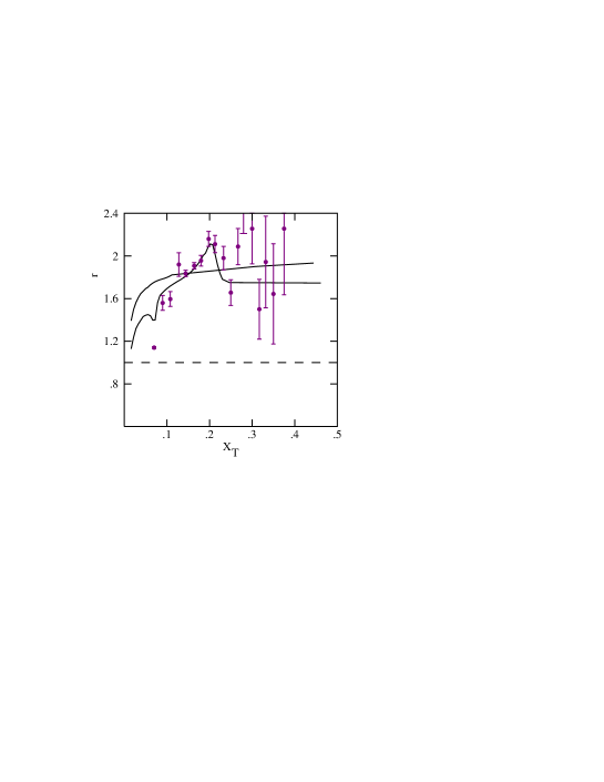
Figure 30: CDF data for the scaling ratio of the inclusive jet transverse energy cross section at $630GeV$ relative to $1.8TeV$ compared to the fit with a light gluino plus $133GeV$ squark and to the standard model prediction (structureless curve). The data has been moved up by $20\%$ consistent with the systematic errors in the $630GeV$ data.

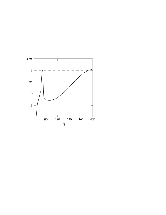
Figure 31: Predicted ratio of the inclusive jet transverse energy cross section with a light gluino and a $133GeV$ squark to that of the standard model for $2TeVp{\overline{p}}$ collisions.

Figure 32: Predicted scaling ratio of the inclusive jet transverse energy cross section at $1.8TeV$ relative to $2TeV$ for a) light gluino only (no squark) and b) light gluino plus $133GeV$ squark. The dash-dotted curve shows the standard model prediction.

XIII Detection of Long-Lived Particles in Run II with DØ

D. Cutts and G. Landsberg

XIII.1 Physics motivation

Long-lived neutral or charged massive particles appear in many extensions of the MSSM. There are two main scenarios which result in a long lifetime of some of the SUSY partners. In the models that predict a degenerate mass spectrum of SUSY particles, light SUSY partners might be stable or long-lived, since the phase space would not allow for strong decays modes. Some models (see sections

It is particularly interesting if the NLSP is long-lived, since the observation of such an NLSP might not be doable via standard decay signatures expected for short-lived SUSY particles. As an example, many MSSM extensions predict degenerate mass spectrum of the neutralinos, in which case the following radiative decay could be a dominant decay mode of the second-lightest neutralino:

$$\tilde{\chi^{0}_{2}}\rightarrow\tilde{\chi}^{0}_{1}\gamma.$$ (44)

Being electromagnetic, this decay mode is suppressed, and for fine splitting between the masses of the two lightest neutralinos, the decay constant could be small enough to result in a long-lived $\tilde{\chi}^{0}_{2}$.

Among other models which allow for a long-lived NLSP, are the GMSB scenarios in which a neutral NLSP (usually a neutralino) radiatively decays into a gravitino LSP:

$$\tilde{\chi}^{0}_{1}\rightarrow\gamma\tilde{G},$$ (45)

or a charged NLSP (usually the right-handed stau, $\tilde{\tau}_{R}$) decays into a $\tau$ and a gravitino NLSP:

$$\tilde{\tau}_{R}\rightarrow\tau\tilde{G}$$ (46)

In the GMSB scenarios the gravitino mass is given by (see, e.g., Feng ):

$$M_{\tilde{G}}=\sqrt{\frac{8\pi}{3}}\frac{F}{M_{P}},$$

where $F$ is the vacuum expectation value of the dynamical supersymmetry breaking, and $M_{P}$ is Planck mass. Since most of the GMSB models predict $F\sim 10^{[}14]$ GeV², and $M_{P}\sim 10^{19}$ GeV, the gravitino is expected to be very light. The fact that the gravitino interacts with matter only weakly, could make the decays (45) and (46) very slow. For example, the $c\tau$ for the decay (46) is given by Feng :

$$c\tau\approx 10~{}\mbox{km}\times\langle\beta\gamma\rangle\times\left[\frac{\sqrt{F}}{10^{7}~{}\mbox{GeV}}\right]^{4}\times\left[\frac{100~{}\mbox{GeV}}{m_{\tilde{\tau}_{R}}}\right]^{5},$$

and could be very large.

Other models (see, e.g. Section II) consider cascade decays of the SUSY particles that can also result in displaced vertices. Massive charged long-lived SUSY particles are expected in SUSY models with chargino LSP Feng1 where the lightest neutralino and chargino are nearly degenerate in mass. Similar degeneracy automatically occurs in superstring-inspired models of SUSY breaking Randall . Weakly interacting bound states of gluino LSP also act as long-lived massive particles (see, e.g. Section III).

Generally speaking, in different SUSY models, the $c\tau$ of the charged or neutral long-lived particles can be from subatomic distances to many kilometers.

XIII.2 Detection of the Delayed Decays

Detection and identification of long-lived particles depend on the decay path and the charge of this particle. A typical collider detector, e.g. the upgraded DØ apparatus D0Upgrade , has an inner Silicon Microstrip Tracker (SMT), capable of identifying secondary vertices from long-lived particle decays. The silicon detector is surrounded by a less precise Central Fiber Tracker (CFT), which is enclosed in the calorimeter. The calorimeter is surrounded by the muon system. Typical outer radii of the vertex detector, central tracking detector, calorimeter, and the muon system are $\sim 10$, 100, 200, and 1000 cm, respectively.

In the case of the charged long-lived particles, one can identify the secondary decay vertex in the silicon vertex detector for $\gamma c\tau$ between $\sim 0.1$ cm and $\sim 10$ cm. Since we expect SUSY particles to be heavy, in what follows we will assume $\gamma\approx 1$, i.e. $\gamma c\tau\approx c\tau$. Both the CDF and DØ experiments will be capable of identifying such secondary vertices and possibly trigger on them. For 10 cm $\lesssim c\tau\lesssim 100$ cm, the charged long-lived particle will predominantly decay inside the outer tracking volume. The resulting characteristic signature is a kink in the outer tracker and large $dE/dx$ in the silicon vertex tracker and the inner layers of the outer tracker, typical for a slow-moving charged particle. While triggering on the kinks in the outer tracker won’t be possible in Run II, there is a good chance that such kinks can be found offline, if the event is accepted by one of the standard triggers. Since a massive slow moving particle still has a significant momentum, one would likely trigger on such events using a single high-$p_{T}$ track trigger, or a designated $dE/dx$ trigger. For 100 cm $\lesssim c\tau\lesssim 200$ cm, the charged long-lived particle will decay inside the calorimeter, giving a jet-like energy deposition inside it. Identification of these particles will therefore rely on the fact that such a jet has only one track pointing to it (similar to one-prong $\tau$-decays); moreover, this track will have high $dE/dx$. In the case of the DØ detector, an additional $dE/dx$ measurement in the preshower detector can be used to aid the identification of such particles both offline and at the trigger level. A single high-$p_{T}$ track trigger, a designated $dE/dx$ trigger, or a $\tau$-trigger could be used to trigger on such events. Finally, for $c\tau\gtrsim 200$ cm, the long-lived particle will look stable from the point of view of the detector, and its identification will rely on a high $dE/dx$ track in the silicon vertex detector, the outer tracker, the calorimeter, and the muon system (if the $c\tau$ exceeds it outer radius). An additional time-of-flight (TOF) information from a designated TOF system (CDF) or muon system scintillators (DØ) could be used to trigger on such events and identify them offline. To summarize, both the CDF and DØ detectors will have very good capabilities for searches for charged long-lived particles with lifetimes from a few tens of picoseconds to infinity. Identification of the slow-moving particles using $dE/dx$ techniques in the case of the DØ detector is discussed in more detail in Section XIII.4.

The situation is much more complicated for a neutral weakly interacting particle. First of all, if such a particle decays outside of the calorimeter, it can not be detected, and will look like a missing $E_{T}$ in the event, i.e. like the LSP. It’s unlikely that one could identify the presence of a long-lived NLSP in such events, but it still might be possible to identify these events as the non-SM ones. If events with such a signature are found in Run II, one could conceivably install a wall of scintillating detectors far away from the main detector volume and try to look for a photon from the radiative decay in this additional scintillator Gunion . For the purpose of this report, however, we will focus only on the case of $c\tau<2$ m, which roughly coincides with the outer radius of the DØ calorimeter. The detection technique for such decays relies heavily on the fine longitudinal and transverse segmentation of the preshower detector and the calorimeter, which is an essential and unique feature of the DØ detector.

The signature for the radiative decay of a long-lived particle (e.g., (45) or (44)), is a production of a photon with a non-zero impact parameter. If there was a way to identify the point of photon origin, one could single out such a delayed radiative decay corresponding to a very distinct and low background topology. As is shown in Section XIII.3, the DØ calorimeter information, combined with the preshower information, can be used to achieve a very precise determination of the photon impact parameter. This technique would allow to identify long-lived neutral particles with 10 cm $\lesssim c\tau\lesssim 100$ cm, in the case of the upgraded DØ detector. The detectable $c\tau$ range can be further extended by a factor of two by looking for the photons from the radiative decay in the DØ hadronic calorimeter. The signature for such photons would look like a “hot cell,” i.e. an isolated energy deposit in one or two hadronic calorimeter cells. The reason that the EM energy deposition in the calorimeter is so isolated is the fact that each hadronic calorimeter cell contains many radiation lengths and completely absorbs an EM shower. The main background for this signature is production of high-$p_{T}$ $K_{S}^{0}$-mesons which decay into a pair of $\pi^{0}$’s corresponding to the 4$\gamma$ final state. Since the $K_{S}^{0}$ is significantly boosted, these four photons are highly collimated and will be identified as a single EM shower in the calorimeter. For a typical $K^{0}_{S}$ momentum of 25 GeV, which corresponds to $\sim 20$ GeV $E_{T}$ of the resulting $4\gamma$ system, the $\gamma c\tau$ is about 130 cm, i.e. most of the $K^{0}_{S}\rightarrow 4\gamma$ decays will occur in the hadronic calorimeter. This background, however, can be well predicted and also has a well defined $r$-dependence, where $r$ is the radial distance of the “hot cell” from the detector center. We therefore expect this background to be under control in Run II. Thus, the upgraded DØ detector will have unique capabilities for searching for neutral long-lived particles with 10 cm $\lesssim c\tau\lesssim 2$ m.

Both the CDF and DØ could also explore the 0.1 cm $\lesssim c\tau\lesssim 10$ cm range by looking for a conversion of the photon from a radiative decay in the silicon vertex detector. If the photon converts, one can determine its direction and the impact parameter fairly precisely by looking at the tracks from the $e^{+}e^{-}$-pair. One, however, would pay a significant price for being able to explore this region of $c\tau$, since the probability of photon conversion in the silicon vertex detector is only a few per cent. CDF could in principle use the conversion technique to explore higher values of the $c\tau$ by looking for conversions in the outer tracking chamber. However, due to the low conversion probability the sensitivity of the CDF detector in this region is by far lower than that of the DØ detector.

Apart from being crucial for the study of physics with delayed radiative decays, the DØ detector ability for photon pointing is very attractive from other points of view. In the high luminosity collider environment the average number of interactions per crossing exceeds one. (It can be as high as five, for the 396 ns bunch spacing expected at the beginning of Run II.) Therefore, each event will generally have several primary vertices with only one being from the high-$p_{T}$ interaction of physics interest, and the others being due to minimum bias $p\bar{p}$ collisions. The presence of multiple vertices creates a problem in choosing the right one for determination of the transverse energies of the objects. Photon pointing can solve this problem. It is especially important at the trigger level when the information about all the objects in the events is not generally available, and therefore high-$p_{T}$ objects which produce tracks in the tracking chambers can not always be used to pinpoint the hard scattering vertex. In some cases, for example the $\gamma+\mbox{${\hbox{$E$\kern-6.00006pt\lower-0.43057pt\hbox{/}}}_{T}$}$ final state, there are no objects with tracks at all, so there is no way to determine what vertex the photon originated from without utilizing the calorimeter-based pointing. Not knowing which vertex is the one from high-$p_{T}$ collision results in the object $E_{T}$ mismeasurement, which is especially problematic for missing transverse energy calculations. Indeed, ${\hbox{$E$\kern-6.00006pt\lower-0.43057pt\hbox{/}}}_{T}$ calculations rely heavily on the vertex position and picking the wrong one may result in significant missing transverse energy calculated in the event which in fact does not have any physics sources of real ${\hbox{$E$\kern-6.00006pt\lower-0.43057pt\hbox{/}}}_{T}$. Not does only this affect physics analyses for topologies with ${\hbox{$E$\kern-6.00006pt\lower-0.43057pt\hbox{/}}}_{T}$, especially the $\gamma+\mbox{${\hbox{$E$\kern-6.00006pt\lower-0.43057pt\hbox{/}}}_{T}$}$ one, but it also results in a worsening of the ${\hbox{$E$\kern-6.00006pt\lower-0.43057pt\hbox{/}}}_{T}$ resolution, hence a slower turn-on of the ${\hbox{$E$\kern-6.00006pt\lower-0.43057pt\hbox{/}}}_{T}$-triggers and ergo higher trigger rates. It is, therefore, very important to have a way of telling the high-$p_{T}$ primary vertex, and photon pointing is the only way of doing this in the $\gamma+\mbox{${\hbox{$E$\kern-6.00006pt\lower-0.43057pt\hbox{/}}}_{T}$}$ case.

Subsequent sections contain technical detail on the high-$dE/dx$ and delayed photon identification.

XIII.3 Photon Pointing at DØ

The importance of photon pointing was appreciated in some Run I analyses, particularly the studies of $Z(\nu\nu)\gamma$ Zg and $\gamma\gamma$ monopoles . We have utilized the fine longitudinal segmentation of the DØ EM calorimeter (which has four longitudinal layers) by calculating the c.o.g. of the shower in all four layers independently and then fitting the four spatial points to a straight line in order to determine the impact parameter and the $z$-position of the photon point-of-origin EMVTX (see Fig. 33). The algorithm used for the c.o.g. finding is based on a logarithmic weighting of the energy deposition in the EM calorimeter cells which belong to the EM shower. The spatial resolution of the c.o.g. finding algorithm in four calorimeter layers averaged over central (CC) and forward (EC) rapidity range, as well as the geometrical parameters of the calorimeter layers are given in Table 7. This study resulted in an algorithm, EMVTX EMVTX , that has been used in several DØ analyses involving photons Zg ; monopoles .

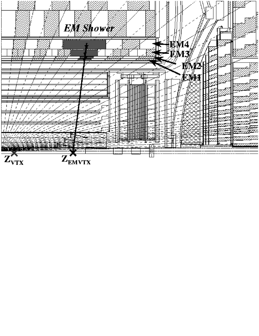
Figure 33: Side-view of the DØ calorimeter illustrating the application of the EMVTX algorithm.

Table 7: Geometry and average resolutions in the preshower detectors and the EM calorimeter layers.

Quantity	Preshower	EM1	EM2	EM3	EM4
Central Region
$\langle R\rangle$ c.o.g.	73.0 cm	85.5 cm	87.4 cm	91.8 cm	99.6 cm
$\sigma_{z}$	2.5 mm	20 mm	20 mm	7.0 mm	15 mm
$\sigma_{r\phi}$	1.5 mm	17 mm	17 mm	3.5 mm	7.5 mm
Quantity	CPS	EM1	EM2	EM3	EM4
Forward Region
$\langle|Z|\rangle$ c.o.g.	142.0 cm	171.7 cm	174.2 cm	179.2 cm	189.7 cm
$\sigma_{r}$	1.5 mm	8.0 mm	8.0 mm	1.5 mm	3.5 mm
$\sigma_{r\phi}$	2.5 mm	7.0 mm	7.0 mm	1.0 mm	2.8 mm

In order to study the improvement of photon pointing made possible by the utilization of the fine spatial resolution of the preshower detector, we have written a toy Monte Carlo (MC) simulation package which takes into account detector geometry, position error in calorimeter and preshower, as well as the primary vertex distribution. First, we compare the resolution obtained from the toy MC with the actual distributions obtained from $W\rightarrow e\nu$ events collected in Run I. For electrons from $W$-events it is possible to determine the point of origin by using track information, which is quite precise. The difference between the $z$ position of the vertex obtained from tracking and from electron pointing as well as the signed impact parameter for the electron obtained by pointing are shown in Fig. 34, for central electrons. (The positive sign corresponds to the impact parameter to the right of the center of the detector observed from the EM cluster location.) The distributions are fitted with Gaussian functions with the widths of $\sigma_{z}=14.0$ cm and $\sigma_{r}=9.5$ cm, as determined from toy MC. The data agrees well with the MC predictions and also appears Gaussian. An analogous comparison for forward electrons is shown in Fig. 35. The corresponding resolutions are $\sigma_{z}=17.0$ cm and $\sigma_{r}=4.5$ cm. The resolution on impact parameter improves in the forward region because the physical size of the calorimeter cells becomes smaller with an increase in $|\eta|$. In the $z$-direction, this effect is compensated by the small angle of the cluster pointing, which dilutes the $z$-resolution.

Figure 34: Comparison of (a) the error on the $z$-position of the vertex, and (b) the signed impact parameter from Run I $W\rightarrow e\nu$ data, with the results of toy simulations, for central electrons.

Figure 35: Comparison of (a) the error on the $z$-position of the vertex, and (b) the signed impact parameter from Run I $W\rightarrow e\nu$ data, with the results of toy simulations, for forward electrons.

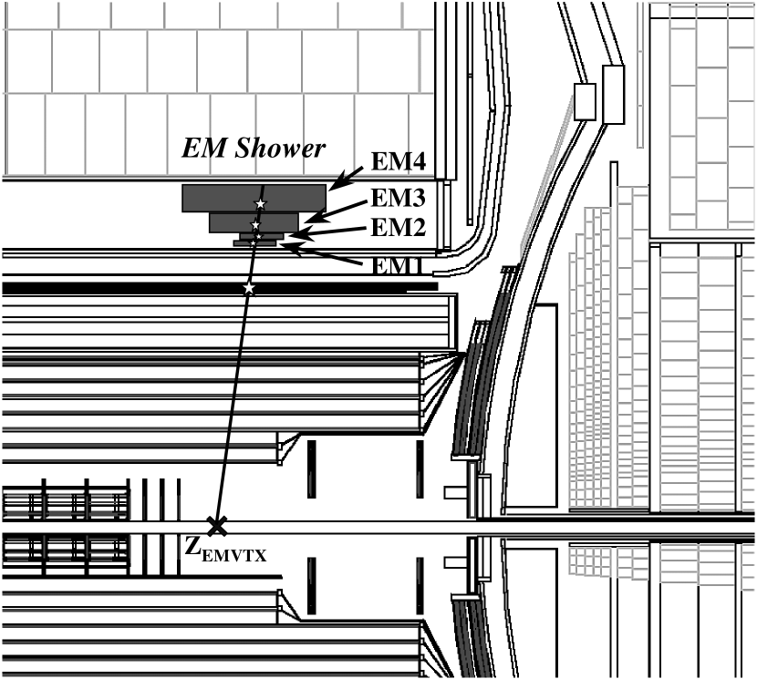
Figure 36: Side-view of the DØ calorimeter illustrating how the EMVTX algorithm works.

Figure 37: Run II simulation of (a) the error on the $z$-position of the vertex, and (b) the signed impact parameter, for central photons.

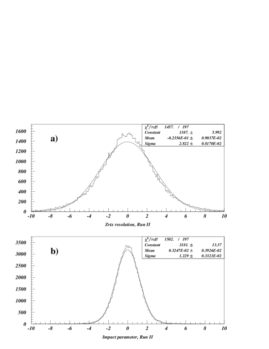
Figure 38: Run II simulation of (a) the error on the $z$-position of the vertex, and (b) the signed impact parameter, for forward photons. The slightly non-Gaussian shape is due to the change in the pointing resolution as a function of the photon rapidity.

The central and forward preshower detectors of the DØ Upgrade provide a precision measurement of the photon cluster position. The resolution for a typical EM shower perpendicular to the preshower strip is $\sim 1$ mm. Taking into account the crossing angle between the $u$- and $v$-planes in the preshower detectors, the following resolutions in $r\phi$ and $z$ ($r$) can be obtained: $\sigma_{r\phi}=1.5$ mm, $\sigma_{z}=2.5$ mm (CPS) and $\sigma_{r\phi}=2.5$ mm, $\sigma_{r}=2.5$ mm (CPS). As one can see, the preshower cluster position measurement is superior to that obtained from the EM calorimeter; its position is also spatially separated from that in the calorimeter, as seen in Fig. 36.

With the additional position measurement coming from the preshower detectors, the following pointing resolutions can be obtained for central and forward photons in Run II: $\sigma_{z}=2.2$ cm, $\sigma_{r}=1.4$ cm (CC, see Fig. 37) and $\sigma_{z}=2.8$ cm, $\sigma_{r}=1.2$ cm (EC, see Fig. 38). A very significant improvement in photon pointing (by a factor of six) is achieved by utilizing the additional position measurement provided by preshower detectors.

The implementation of the photon-pointing algorithm can be done as early as at the trigger Level 3. An approximate algorithm that uses only the c.o.g. of the EM shower in the preshower and in the third layer of the EM calorimeter could be used to decrease the amount of calculations and, hence, the decision-making time. Monte Carlo simulations show that the impact parameter and $z$-resolutions for a simplified algorithm are only 10% worse than those obtained by complete five-point fit, which is quite satisfactory for trigger purposes. Having the precise vertex information from photon-pointing for photon triggers at Level 3, we will also recalculate the ${\hbox{$E$\kern-6.00006pt\lower-0.43057pt\hbox{/}}}_{T}$based on this vertex, and that would significantly improve the turn-on of the ${\hbox{$E$\kern-6.00006pt\lower-0.43057pt\hbox{/}}}_{T}$part of less inclusive triggers which would require an EM cluster and ${\hbox{$E$\kern-6.00006pt\lower-0.43057pt\hbox{/}}}_{T}$.

XIII.4 Detection of Slow-Moving Massive Charged Particles in DØ

As described in Section XIII.2, long-lived charged particles have a variety of characteristics which enable their identification, particularly in the analysis stage when the event’s complete data set is available. Depending on the lifetime, a combination of time-of-flight, ionization ($dE/dx$) in several different detectors, and the muon-like penetration of a high momentum, isolated track all can be employed, with the additional presence of a kink where there is a decay within the detector volume. Even though discovery at the analysis stage seems possible, triggering is really crucial, if heavy stable particles produced at the Tevatron are to be detected. In this section we discuss the possibilities for triggering, and in particular, the use of $dE/dx$ in the hardware trigger as a tool for detecting these objects.

The DØ trigger system is hierarchical, with 3 levels, each level passing a small subset of the events it examines to the next level for further analysis. Thus Level 1 has a high input rate and examines a limited amount of information in making its decision, while subsequent levels have progressively lower input rates and spend longer analyzing more data. At Level 3, all the data digitized for the event is available and the selection is made running software algorithms written in high level code and derived from the offline analysis. We expect that the massive stable particles will be sufficiently rare, and their characteristics clear, such that separating candidates at Level 3 will be straight forward. However, we need to understand how to identify these events in the hardware triggers so that they survive to Level 3.

For Level 1 several tools are available to detect a massive stable particle. The Central Fiber Tracker provides track candidates binned in momentum to which it can apply an isolation criteria Yuri . The CFT has 80 trigger segments independently processed by the trigger. For a heavy stable particle one can select a high $p_{T}$ track with no other tracks in the home and adjacent segments, imposing an isolation of $\pm 6.75^{\circ}$ in azimuthal angle Yuri . Association of a muon with such a track would provide an efficient Level 1 trigger for massive stable particles, produced centrally and in isolation.

An additional tool KJ at Level 1 is the measurement of the time of flight (TOF) from scintillators associated with the muon detector and used primarily to reduce background in the large area muon detector from cosmic ray and beam associated accidentals. These counters cover much of the area just outside the calorimeter, inside the first (“A”) layer of muon detectors, and completely outside the detector, on top of the muon “C” layer planes. Electronics associated with the scintillation counters provides both a trigger gate and a TOF gate, thus giving time windows relative to the interaction time. Scintillator hits received within the TOF gate will have the time of flight measurement digitized and saved with the data, assuming the event otherwise passes Level 1. Typically the TOF gate will be set sufficiently wide to accept slow moving particles, namely at least 100 nsec. To contribute to the Level 1 trigger, however, the scintillator hit must occur within the trigger gate, which is necessarily much shorter (of order 25 nsec) because of the high rate of accidentals, particularly in the “A” layer counters. It may be possible to run with a considerable wider trigger gate for the “C” layer counters, given the lower expected accidental rate in these counters. In this case, TOF from the muon system would provide a useful tool for Level 1 triggering on slow particles. Given a Level 1 trigger, generated either through TOF or through an isolated stiff CFT track, the TOF data will be a useful tool for the Level 2 and Level 3 triggers.

Beyond Level 1, the new Silicon Microstrip Tracker provides interesting possibilities for triggering on slow moving particles. Since energy loss of a slow moving particle drops as $1/\beta^{2}$ as a function of its velocity, the excellent $dE/dx$ energy resolution of the silicon chip provides a good handle for offline identification. For example, the energy deposited in one silicon layer is shown in Fig. 39, as measured in a test beam Maria . More importantly for the detection of slow moving particles, there are possibilities to exploit these measurements at the trigger level, with recent approval of the DØ Silicon Tracker Trigger (STT) STT as a component of the Level 2 trigger system. The hardware design for the STT may allow for the inclusion of several additional backplane lines to carry $dE/dx$ information along with the other data associated with each cluster of hits Uli . We have studied the basic capabilities of such trigger hardware to explore its potential for slow particle identification.

Figure 39: Energy deposition in one layer of the Silicon Microstrip Tracker in ADC counts, as measured in the test beam.

Our simulation of the STT slow particle trigger is based on a simple Monte Carlo generator which returns an ADC value appropriate for the spectrum shown in Fig. 39. We assume that two backplane lines per SMT hit are available, and we encode each ADC value into these two bits of data, or four bins. After trying various values for the three bin edges, we have chosen to define the bins by those ADC values below which lie 67%, 95%, and 99% of the data. These cutoffs correspond to 38, 75, and 105 ADC counts (see Fig. 39). The STT Level 2 trigger processor finds tracks using four layers of silicon; so, in our model, the hardware would provide four samples of this two bit $dE/dx$ data for each track. At this point the trigger would use some algorithm to combine the four samplings most advantageously. The major concern for the correct identification of a slow moving particle is the likelihood of false signals from a minimum ionizing particle (MIP), due to an occasional response in the very long tail of the Landau energy loss distribution. Based on a few studies, our preliminary suggestion is simply to sum the three lowest values, rejecting the largest ADC count of the four. The data then would provide a parameter, related to a $dE/dx$ of the particle in the silicon tracker, which we call “slowness,” and which has 10 possible values (0..9). From our simulation we derive the distribution in slowness for a $\beta=1$ particle (equivalent to the test beam pion), as shown in Fig. 40.

Figure 40: Distribution of slowness for massive particles with $\beta=0.4$ and 0.7, and test beam particles with $\beta=1.0.$

The ADC response to the passage of a slow moving particle will be similar to the ADC distribution of Fig. 39 scaled by the factor $1/\beta^{2}$. However, because of the very different kinematics (the slow moving particle is massive, typically 150 GeV) the energy loss distribution will have a less pronounced Landau tail. We make a very conservative assumption and use only the Gaussian component in generating ADC values for massive slow moving particles. Several resulting distributions in our $dE/dx$ trigger parameter, “slowness,” for particles with $\beta=0.4$ and $\beta=0.7$, are included in Fig. 40. There is a clear separation in this parameter compared to the $\beta=1$ distribution.

To estimate the effectiveness of the STT $dE/dx$ trigger we consider a selection which tags as a slow particle those whose “slowness” is greater than or equal to some value. We vary this selection to study the efficiency for slow particles (at highest possible $\beta$) while maintaining a strong rejection against $\beta=1$ particles. Figure 41 shows the acceptance as a function of a particle’s velocity, for events with slowness $>4$. The appearance of a few $\beta=1$ particles but not other high $\beta$ events reflects the conservative use, for massive particles, of a Gaussian ADC response, rather than the Landau distribution, which is used to generate the ADC values from a MIP.

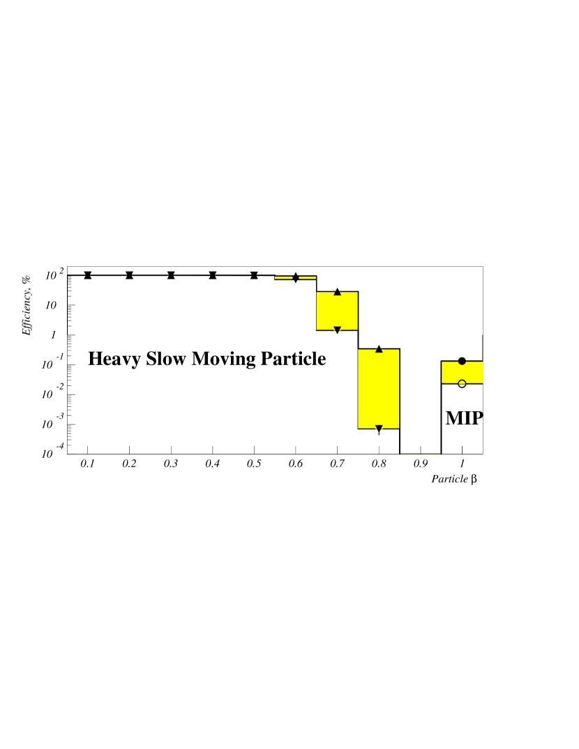
Figure 41: Efficiency as a function of particle $\beta$ for events with slowness $>3$. The open histogram corresponds to the case without angular smearing; the filled area shows the change when angular smearing of $\pm 45^{\circ}$ is taken into account.

Figure 42: Efficiency as a function of particle $\beta$ for the events with redefined slowness a) $>7$; b) $>8$. Angular smearing of $\pm 45^{\circ}$ is taken into account.

Despite the intent to trigger only on centrally produced objects, tracks will tend to be inclined to the silicon, increasing and broadening the $dE/dx$ response. In fact, the STT hardware will search for track candidates from adjacent barrels; so that tracks may be inclined to the normal by as much as $45^{\circ}$ although the STT will have no information about this angle. We have modeled the effect of inclined tracks by scaling the appropriate ADC response by $1/\cos\theta$, where $\cos\theta$ is generated uniformly between .707 and 1.0, or by $\eta$, where $\eta$ is generated uniformly between 0 and 0.88. The differences between smearing based on $\cos\theta$ and that based on $\eta$ are small. We present here results using $\cos\theta$ smearing for the centrally produced massive stable particles and $\eta$ smearing for the $\beta=1$ background. As seen in Fig. 41, the effect of the variation in ADC response due to track inclination is only a small reduction in the rejection for $\beta=1$ particles; moreover, this effect helpfully raises the cutoff in $\beta$ for massive particles. Overall, this smearing does not appear to affect the STT “slowness” trigger significantly. Including track inclination, the study suggests that the STT Level 2 $dE/dx$ trigger would provide a fully efficient tag for slow particles up to $\beta=0.7$ with an acceptance of $\beta=1$ particles less than $2\times 10^{-3}$.

Because of its excellent rejection for $\beta=1$ particles, the Level 2 $dE/dx$ trigger will be a good means to select slow moving particles, independent of other criteria such as TOF or track isolation. However, if the particle is sufficiently long-lived to traverse the entire detector, it may be possible to relax the $dE/dx$ requirement. We have studied the effect of modifying the hardware ADC sampling, to explore widening the acceptance of heavy particles in $\beta$ at the expense of $\beta=1$ rejection. There is good physics motivation in doing so, as some GMSB models predict the production of heavy stable particles with $\beta$ in the range 0.8-0.9 Jianming . Using ADC bins with edges corresponding to 50%, 68%, and 90% of the distribution, we find good acceptance for massive particles at high $\beta$, as shown in Fig. 42, with rejection factors between 20 and 100, for $\beta=1$ particles.

The above study illustrates the potential of a STT $dE/dx$ trigger. It does assume that the ADC distribution for a MIP is as seen in the test beam, and that differences in the silicon chip response over the detector won’t significantly affect this distribution. The study suggests that track inclination may not be a serious problem. Further, the “slowness” flag derived with the STT from $dE/dx$ can in Level 2 be combined with other information (as of a straight, non-oblique and isolated muon) to provide a global Level 2 trigger. In summary, it seems promising that the STT could provide very useful $dE/dx$ information early in a slow particle’s lifetime, which can be combined with other data to create an efficient trigger for these interesting objects.

XIV Searches for Beyond the MSSM Phenomena at CDF

M. Chertok

Two remarks motivate the discussion to follow. First, if the LSP is charged and has an appreciable lifetime (or is stable), it can be detected in a search for charged massive particles (CHAMPs). Second, while the MSSM makes no predictions regarding the possibility of extra quark families, there is no theoretical reason against them mckay .

CDF has performed searches for these phenomena using data taken with the Run I detector det . Upgrades of both the detector and Tevatron are currently underway tdr . These will provide substantial enhancements for these and other searches in Run II, scheduled to begin in 2000. During this run, CDF II will collect roughly 2 ${\rm fb}^{-1}$ of data at $\sqrt{s}=2\mbox{$\;{\rm TeV}$}$, corresponding to twenty times the present statistics. The 10% increase in energy corresponds to a 40% increase in the $t\overline{t}$ yield, and similarly will aid new phenomena searches.

Although the LEP data at the $Z^{0}$ pole exclude extra fermion generations with light neutrinos LEP , models including fourth family quarks have received recent theoretical attention mckay ; four_theory . CDF performs three complementary searches for such quarks, described below.

XIV.1 Search for long-lived parent of the $Z^{0}$

CDF performs a general search for long-lived particles decaying to $Z^{0}$ bosons lxy . One example is a $b^{\prime}$ quark decaying via a FCNC to a $b$ quark and a $Z^{0}$. This decay can dominate (depending on the $b^{\prime}$ mass) but may lead to a long lifetime. Another example is low-energy symmetry breaking models with SUSY ambrosanio that predict the decay $\mbox{$\tilde{\chi}_{1}^{0}$}\rightarrow\mbox{$Z^{0}$}\tilde{G}$ with a long lifetime due to the small coupling constant of the gravitino.

The technique for this search is to select $e^{+}e^{-}$ pairs from $Z^{0}$ decay and search the transverse decay length distribution for evidence of $Z^{0}$ bosons originating at a displaced vertex. Electrons ($e^{+}$ or $e^{-}$) are required to satisfy $\mbox{$E_{T}$}>20\mbox{$\;{\rm GeV}$}$, $\mbox{$p_{T}$}>15\mbox{$\;{\rm GeV}/c$}$, and $|\eta|<1$, with the pair reconstructing to the $Z^{0}$ mass: $|M_{ee}-M_{\mbox{$Z^{0}$}}|<15\mbox{$\;{\rm GeV}/c^{2}$}$. Quality cuts are imposed to reduce the effects of misreconstructed tracks. The $e^{+}$ and $e^{-}$ are required to originate from a common vertex, and nearly collinear tracks are removed by requiring $|\Delta\phi-\pi|>0.02$. A high-purity sample of $J/\psi\rightarrow\mu^{+}\mu^{-}$ is used to check that these cuts do not introduce lifetime biases. In 90 ${\rm pb}^{-1}$, 703 events pass the full selection.

The reconstructed transverse decay length $L_{xy}$ distribution from these events is clustered around the origin, as expected, and can be modeled with a central gaussian and tails due to tracking errors. The negative $L_{xy}$ region is used to estimate the background from tracking errors and select an $L_{xy}$ cut which is then used to search for a signal in the positive $L_{xy}$ region. A cut of $\mbox{$L_{xy}$}>1mm$ is chosen, which corresponds to an expectation of $\leq$ one event based on the central gaussian. There is one candidate event with $\mbox{$L_{xy}$}>+1mm$. As the data are consistent with background levels, limits are derived as shown in Figure 43. The left figure shows the model independent cross section times branching ratio limit as a function of the lifetime, as well as a limit (insert) for the case of $\mbox{$b^{\prime}$}\rightarrow b\mbox{$Z^{0}$}$. In this case two jets with $\mbox{$E_{T}$}>10\mbox{$\;{\rm GeV}$}$ and $|\eta|<2$ are additionally required and the $L_{xy}$ cut is made at $0.1mm$. Also shown (right) is the resulting limit on the $b^{\prime}$ mass as a function of the lifetime.

Plans for the continuation of this analysis in Run II include the addition of the muon channel and an attempt to perform the search using only the outer tracking chamber without the SVX. The former would increase the cross section sensitivity by approximately a factor of two while the latter would flatten out the limit to $\sim 30$ cm. Folding in the other factors for Run II improvements and integrated luminosity, the present cross section limit minimum of 0.5 pb for the model independent case should be reduced to below 5 fb. For the $b^{\prime}$ model, masses up to the top quark mass should be excluded in Run II.

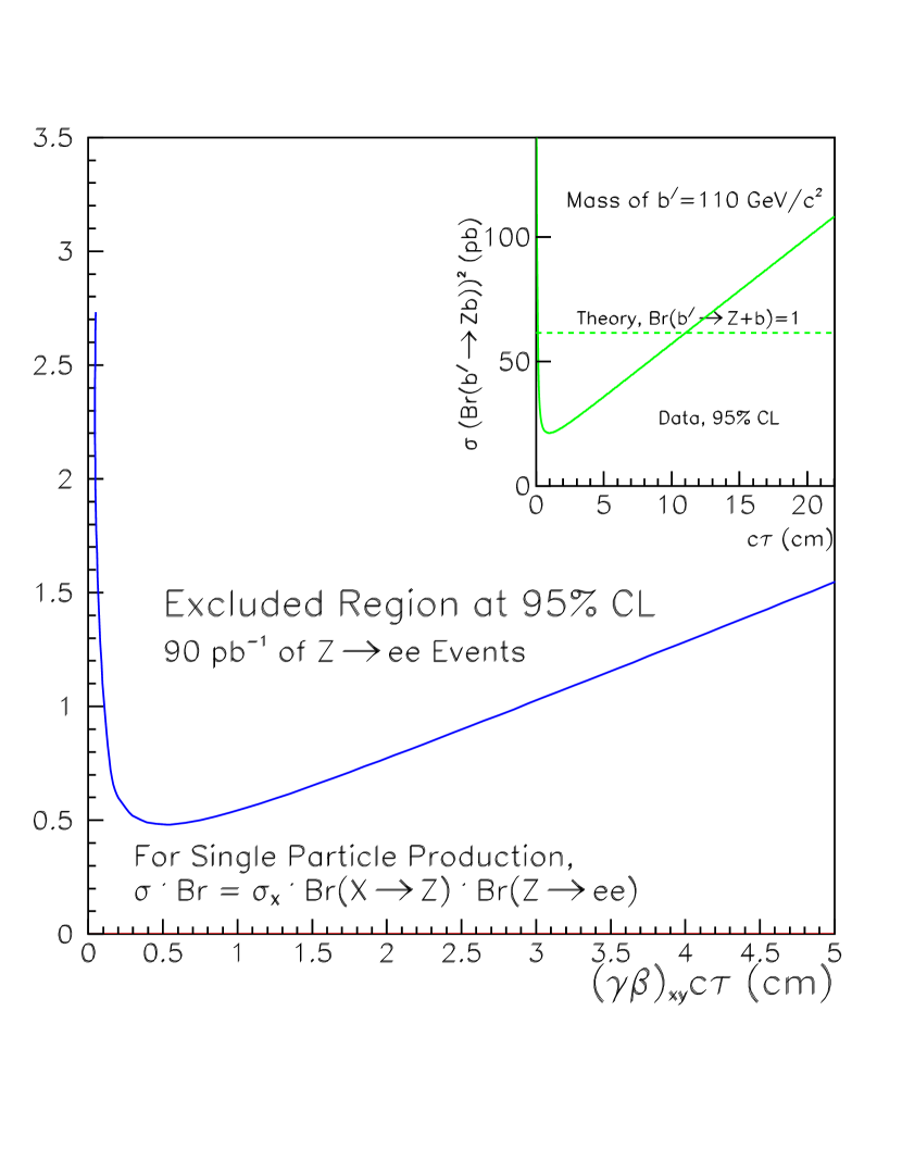
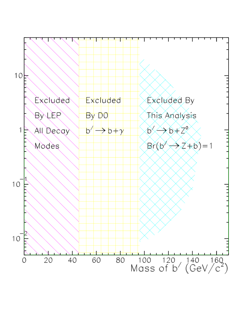
Figure 43: Search for a long-lived parent of the $Z^{0}$. Cross section limit (left) and mass limit (right).

XIV.2 Search for $b^{\prime}\bar{b}^{\prime}\rightarrow\mbox{$Z^{0}$}\mbox{$Z^{0}$}b\bar{b}\rightarrow(\ell^{+}\ell^{-})(q\bar{q})(b\bar{b})$

If a fourth generation $b^{\prime}$ quark is lighter than both $t$ and $t^{\prime}$, then the allowed CC decay $\mbox{$b^{\prime}$}\rightarrow cW^{-}$ is doubly Cabbibo suppressed and the FCNC decay $\mbox{$b^{\prime}$}\rightarrow b\mbox{$Z^{0}$}$ dominates if $m_{\mbox{$b^{\prime}$}}>m_{\mbox{$Z^{0}$}}+m_{b}$. At the Tevatron, $b^{\prime}$ would be pair produced with a cross section like that for top with $b^{\prime}\bar{b}^{\prime}\rightarrow\mbox{$Z^{0}$}\mbox{$Z^{0}$}b\bar{b}\rightarrow(\ell^{+}\ell^{-})(q\bar{q})(b\bar{b})$ as one decay pattern. CDF performs a search for such a $b^{\prime}$ by requiring two electrons consistent with $\mbox{$Z^{0}$}\rightarrow\mbox{$e^{+}e^{-}$}$, with $\mbox{$E_{T}$}(e_{1})>20\mbox{$\;{\rm GeV}$}$, $\mbox{$E_{T}$}(e_{2})>10\mbox{$\;{\rm GeV}$}$, and $75\mbox{$\;{\rm GeV}/c^{2}$}\leq M(\mbox{$e^{+}e^{-}$})\leq 105\mbox{$\;{\rm GeV}/c^{2}$}$. In 87 ${\rm pb}^{-1}$, 6548 events satisfy this electron selection. Three or more jets with $|\eta|<2$ are then required. For the search region $M(\mbox{$b^{\prime}$})<130\mbox{$\;{\rm GeV}/c^{2}$}$, two jets must satisfy $\mbox{$E_{T}$}>15\mbox{$\;{\rm GeV}$}$ while the third can have $\mbox{$E_{T}$}>7\mbox{$\;{\rm GeV}$}$. For $M(\mbox{$b^{\prime}$})>130\mbox{$\;{\rm GeV}/c^{2}$}$, all jets must satisfy $\mbox{$E_{T}$}>15\mbox{$\;{\rm GeV}$}$. Also, the sum of the jet $E_{T}$ for jets with $\mbox{$E_{T}$}>15\mbox{$\;{\rm GeV}$}$ must scale with the $b^{\prime}$ mass in the following way: $\sum\mbox{$E_{T}$}(\mbox{$E_{T}$}(j)>15\mbox{$\;{\rm GeV}$})>M(\mbox{$b^{\prime}$})-60\mbox{$\;{\rm GeV}$}$, motivated by a study of the backgrounds. Finally, one $b$ tag (displaced vertex) using the SVX detector information is required for the event to pass. This final requirement removes the 31 events remaining after the sum $E_{T}$ requirement.

The $b^{\prime}$ signal is generated using HERWIG, with masses in the range $100\mbox{$\;{\rm GeV}/c^{2}$}\leq M(\mbox{$b^{\prime}$})\leq 170\mbox{$\;{\rm GeV}/c^{2}$}$ and passed through the CDF detector simulation program. The efficiency for $\mbox{$Z^{0}$}\rightarrow\mbox{$e^{+}e^{-}$}$ is about 60% and the efficiency for the 3 jet cut ranges from 25% to 66% with $M(\mbox{$b^{\prime}$})$. The main background process for $\mbox{$b^{\prime}$}\rightarrow b\mbox{$Z^{0}$}$ comes from $\mbox{$Z^{0}$}+n\;j$ events, where $n\geq 3$, and are modeled using VECBOS and HERWIG. These events are passed through the CDF detector simulation program and filtered with the same event selection as for the signal.

Presently, this analysis is being finalized and the muon channel is being added. Including this additional acceptance along with the improvements expected in Run II described above, the ultimate sensitivity of the search will reach $M(\mbox{$b^{\prime}$})\simeq M(t)$. It should be noted that the decay $\mbox{$b^{\prime}$}\rightarrow bH$ must be considered in this regime. However, if $H\rightarrow\mbox{$b\overline{b}$}$ is appreciable, much of the signal can be recovered as long as $\mbox{$b^{\prime}$}\rightarrow b\mbox{$Z^{0}$}$ remains large enough to provide triggerable leptons from $\mbox{$Z^{0}$}\rightarrow\mbox{$\ell^{+}\ell^{-}$}$.

XIV.3 Search for long-lived charged massive particles

Several models outside the MSSM predict new charged massive particles (CHAMPs) with appreciable lifetimes. These include fourth generation leptons and quarks, weak ${R_{p}}$ violation, and gauge mediated SUSY breaking models. A strongly interacting CHAMP would have a large cross section (like that for top), which allows large masses to be probed with little background. CDF performs such a search using as a reference model a fourth generation quark with fragmentation to an integer charged meson within a jet.

The technique for this search is to use the large ionization energy loss, ${\rm d}E/{\rm d}x$, in the tracking chambers to tag massive (and therefore slow-moving) particles. Starting with 90 ${\rm pb}^{-1}$ of data from Run I, various tracking cuts for the SVX and central tracker (CTC) are applied to select high quality tracks. Candidate tracks are required to have $|p|>35\mbox{$\;{\rm GeV}/c$}$ and $|\eta|<1$ and to pass ionization cuts in both the SVX and CTC which correspond to requiring $\beta\gamma<0.85$. Finally, a mass is calculated from the momentum and ${\rm d}E/{\rm d}x$ and a sliding cut, $M_{\mbox{${\rm d}E/{\rm d}x$}}>0.6M_{CHAMP}$, is applied for each assumed $M_{CHAMP}$.

The background to this search is due to particles which fake a large ionization signal, mostly from particles whose tracks overlap. The probability of a track faking a signal in both the SVX and CTC is quite low: of the 20K events passing the selection cuts, $12.1\pm 1.8$ tracks from fakes are expected with $\beta\gamma<0.85$. Since the background is higher at low mass, a tighter cut of $\beta\gamma<0.7$ is used for the search region $M_{CHAMP}<100\mbox{$\;{\rm GeV}/c^{2}$}$. With this cut, $2.5\pm 0.8$ tracks from fakes are expected. These background levels agree well with the data as shown in Figure 44. The overall efficiency for this search ranges from 0.75% to 3% as a function of the mass of the CHAMP and is about twice as high for assumed charge $+2/3$ as for charge $-1/3$ due to fragmentation effects. Systematic uncertainties for this analysis are dominated by the uncertainty on interactions of a massive quark in the calorimeter which contribute between 13 and 20% depending upon the assumed quark charge. Figure 44 also shows the resulting cross section limits for this analysis. Comparing these curves to the cross section prediction from PYTHIA, mass limits are obtained at $190\mbox{$\;{\rm GeV}/c^{2}$}$ for $b^{\prime}$ and $220\mbox{$\;{\rm GeV}/c^{2}$}$ for $t^{\prime}$.

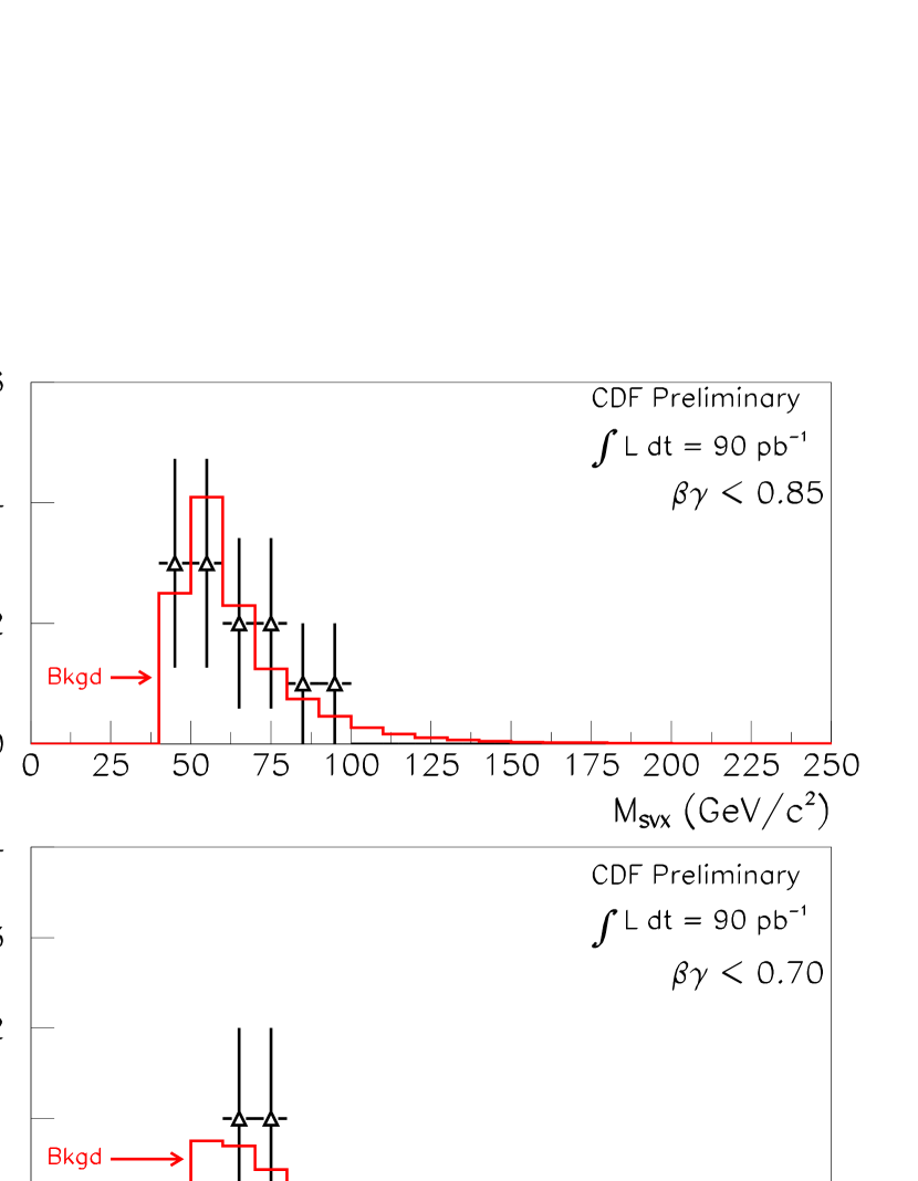
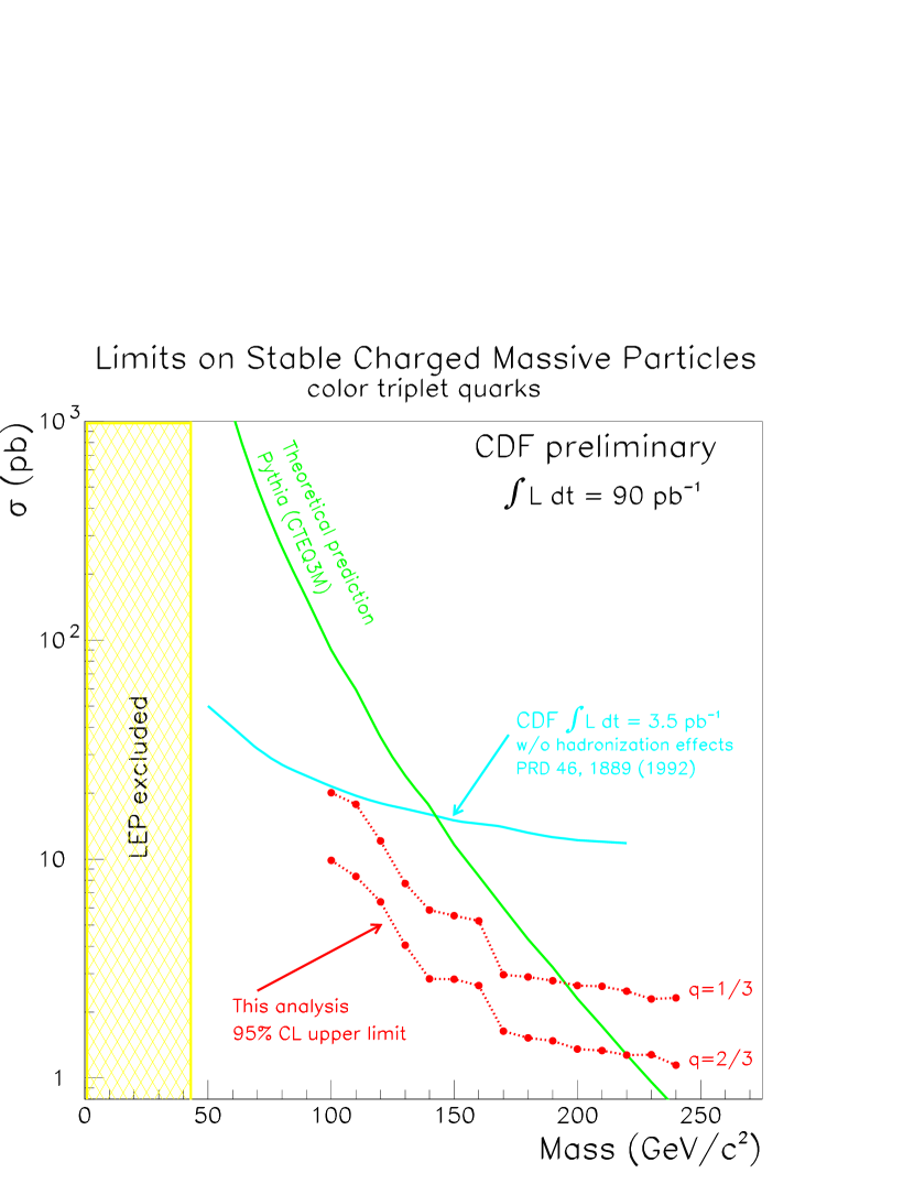
Figure 44: Search for strongly interacting CHAMPs. Masses reconstructed using the SVX for two values of the cut on $\beta\gamma$ (left) and mass limit (right).

In Run II, the CHAMP search will be enhanced by the larger integrated luminosity, higher cross section ($\sim 40\%$), and improved detector acceptance ($\sim 80\%$) due to the new tracking chambers. Moreover, there is a proposal to include a time of flight system to the CDF detector. This will greatly help searches for weakly interacting CHAMPs, and will improve the acceptance for analysis described here by $\sim 50\%$. Combining these factors, the Run II cross section limit for strongly interacting CHAMPs should reduce to 20 fb.

XV New Gauge Bosons at the Tevatron Run II

T. Rizzo

In this section, we provide an overview of the capabilities of the Tevatron to both discover and explore the couplings of new gauge bosons during Run II. The problems associated with identifying a $Z^{\prime}$ once discovered at the Tevatron and issues related to gauge kinetic mixing are also discussed.

XV.1 Conventional $Z^{\prime}$ and $W^{\prime}$ Search Reaches

From the string point of view, new gauge bosons are perhaps one of the most natural extensions of the MSSMlang . The conventional approach in searching for new gauge bosons at hadron colliders is via the Drell-Yan channel where a resonant, on-shell particle is produced which subsequently decays to lepton pairs and is easily observable over any continuum backgroundover . The relevant parameter is thus the product of the production cross section times the leptonic branching fraction, $\sigma B$. Given a particular extended gauge model with a fixed set of couplings and a set of PDF’s there is very little theoretical uncertainty associated with the calculation of this quantity. This implies that search or exclusion reaches are relatively straightforward to establish under the assumption that the new particle can only decay to SM fermion pairs. (It has been shown that if new decay modes are responsible for decreasing the leptonic branching fraction of a $Z^{\prime}/W^{\prime}$ by a factor of 2 it results in a search reach degradation of only $\simeq 50-60$ GeVover at Run II.)

Using the canonical $Z^{\prime}$ from $E_{6}$ as an example and remembering that in this case the fermionic couplings depend on a parameter $\theta$, we show in Fig. 45 both the current exclusion reach from Run I as well as the search reach anticipated from Run II. As the $Z^{\prime}$ couplings vary the search reach also varies over a respectable range of $\simeq 150$ GeV. We also see from this figure that this spread of values is quite typical given the fairly wide set of $Z^{\prime}$ models. Fig. 45 also shows that for a rather wide range of models, including the $E_{6}$ and several Left-Right cases, the search reach scales almost linearly with the log of the integrated luminosity over the range of values relevant for future Tevatron running. In fact a fit to the curves in Fig. 45 reveals that the mass reach scales with luminosity in a quite model-independent manner as $M\simeq M_{0}+91.3\log L-2.68\log^{2}L$ GeV with ${\cal L}$ in $fb^{-1}$ with $M_{0}$ being the only model-dependence.

Figure 45: (Left) Approximate $95\%$CL exclusion limit (dots) from Run I and the anticipated Run II (2 $fb^{-1}$) discovery reach (solid and dash) for a $Z^{\prime}$ arising from $E_{6}$ as a function of the parameter $\theta$ assuming decays to only SM fermions. The two curves represent the results obtained by employing CTEQ4M and MRST98 pdf PDF’s. (Right) Scaling behavior of $Z^{\prime}$ search reaches with integrated luminosity with Run II conditions for seven different extended models. Note the spread of $\simeq 300$ GeV at any given luminosity.

The situation with $W^{\prime}$ search reaches is somewhat different as the canonical example is the Left-Right Modelover . Here not only can the overall $W^{\prime}$ coupling strength, $g_{R}$, differ from that of the $W$ in the SM, $g_{L}$, but the $W^{\prime}$ production cross section may be modulated by a distinct, right-handed CKM matrix, $V_{R}$, and its leptonic decay may involve a massive neutrino, $N$, which can decay in the detector (and thus not appear as missing $p_{t}$, as has been studied by D0d0 ). The variation of the search reach with $V_{R}$, whose structure is a priori unknown, assuming $g_{L}=g_{R}$ and massless neutrinos in the final state is shown in Fig. 46. While the reach in the case $V_{R}=V_{L}$ is $\simeq 1040$ GeV, a serious degradation is experiences as one scans over other possible forms of $V_{R}$ and is easily reduced by more than $20-30\%$ and perhaps as much as $50\%$. Fig. 46 also shows the almost linear scaling of the $W^{\prime}$ search reach with the log of the integrated luminosity in the most naive case; a fit gives to the curve yields $M\simeq M_{0}^{\prime}+76.3\log L-1.86\log^{2}L$ GeV for the reach.

A last point to remember regarding the $W^{\prime}$ reach is that if $N$ is heavier than the $W^{\prime}$ then the Drell-Yan search becomes useless and other modes such as $W^{\prime}\rightarrow WZ$ or $jj$ must be employedother . By scaling existing searches for dijet mass bumps to the energy and luminosity of Run II we have estimated that a $W^{\prime}$ can be discovered in this mode up to masses of 880(970) GeV for a luminosity of 2(30) $fb^{-1}$.

Figure 46: (Left) Distribution of $W_{R}$ search reaches at Run II for $2\times 10^{6}$ different sets of mixing angles and phases in the matrix $V_{R}$. (Right) Search reach as a function of integrated luminosity for $W^{\prime}$ assuming the simplest scenario: $\kappa=g_{R}/g_{L}=1$, $V_{L}=V_{R}$ and essentially massless and stable neutrinos in the final state, for the same PDF’s as in Fig. 45.

XV.2 $Z^{\prime}$ Coupling Determinations and Gauge Kinetic Mixing

If new gauge bosons do indeed exist not far beyond the present limits then they will be easily be discovered during Run II. It then becomes mandatory to address the next question–what $Z^{\prime}$ is it? To do this one needs to measure as many of the various $Z^{\prime}$ properties as possible. While such discussions have taken place for the LHCover , little has been done to address these issues at the Tevatron. We would suppose that if a $\sim 700-800$ GeV $Z^{\prime}$ were discovered accumulating additional luminosity would be easily justified and that at least a few hundreds of events would eventually be collected in both the $e^{+}e^{-}$ and $\mu^{+}\mu^{-}$ channels. Even with this number of events only a few ‘on-peak’ observables will have statistical errors less than $\sim 10\%$ and are thus useful for coupling determinations: ($i$) the familiar forward-backward asymmetry of the final leptons, $A_{fb}$, ($ii$) the longitudinal polarization of one of the $\tau$’s in $Z\rightarrow\tau^{+}\tau^{-}$, $P_{\tau}$, and ($iii$) the relative rate for $Z^{\prime}\rightarrow b\bar{b}$ compared to $\ell^{+}\ell^{-}$, $R_{bl}$x2bb . To see that indeed these three variables, if reasonably well measured, will be able to separate many of the more popular $Z^{\prime}$ models, we compare their correlated values in Fig. 47. Note that the couplings in some cases, such as the Left-Right Model, depend upon the values of a single continuous parameter and so their predictions lie along specific curves and not at unique points. It is clear that a determination of only one of these variables will not be sufficient and generally all three are necessary for good model separation.

Figure 47: Values of $P_{\tau}$, $R_{bl}$ and $A_{fb}$ for a number over of $Z^{\prime}$ models at the Tevatron: conventional $E_{6}$(solid), Left-Right(dash), Un-unified(dots or U), Alternative Left-Right(A), L-R with $\kappa=1$(L), SM couplings(S), Kaluza-Klein excitations($\rm W_{3}$ and B). $M_{Z^{\prime}}=700$ GeV has been assumed. Some models are only shown on one panel as their predictions lie outside the displayed range.

For extended gauge models based on GUTS with only an additional $U(1)^{\prime}$ factor, such as those arising in the $E_{6}$ case, the results shown in Fig. 47 can be too optimistic due to the presence of gauge kinetic mixing(GKM)gkm . GKM is an induced mixing between the $Z^{\prime}$ field strength and that associated with the SM hypercharge that arises due to vacuum polarization-like graphs. At the GUT scale, such graphs cancel since complete GUT matter representations exist. Once the GUT symmetry is broken the matter content of the theory below that GUT scale no longer lies in complete representations. In, e.g., the MSSM only the Higgs doublet superfields remain light whereas their associated color triplet partners remain at the GUT scale. The existence of incomplete representations then leads to GKM via the RGE’s and results in a modification of the naive expectations for the $Z^{\prime}$ couplings at the TeV scale. In the case of conventional $E_{6}$, the $Z^{\prime}$ couples to a charge $Q^{\prime}_{\theta}$, which is dictated by group theory and the value of the $\theta$ mixing parameter. GKM modifies this coupling as $Q^{\prime}_{\theta}\rightarrow\lambda(Q^{\prime}_{\theta}+\delta\sqrt{3\over 5}{Y\over 2})$ where $Q_{em}=T_{3}+{Y\over 2}$. Given a specific matter content of the low energy theory below the GUT scale the parameters $\lambda$ and $\delta$ become calculable via the RGE’s. As far as $Z^{\prime}$ physics at the Tevatron is concerned it is quite fortunate that they cannot take on arbitrary values; for the case of the $\eta$-type model($\theta\simeq 37.76^{o}$) made popular by string theory, $\delta={-1\over 3}$ leads to leptophobia. In this case the $Z^{\prime}$ does not couple to leptons and the standard Drell-Yan search technique fails. This is evident by the ‘hole’ in the search reach shown in Fig. 48. Given a reasonable set of assumptions the matter content of the extended $E_{6}$ model below the GUT scale is not arbitrary, there being only(!) 68 possible sets of superfields to considergkm . For each set the allowed ranges of $\lambda$ and $\delta$ are calculable, as shown in Figs. 4 and 5 of Ref.gkm , from which $Z^{\prime}$ search reaches can be calculated. From this analysis it can be shown that at one loop $-0.286\leq\delta\leq 0.250$ so that exact leptophobia does not happen. From a complete scan of the parameter space the worse case scenario is found to occur for an $\eta$-type model with $\lambda=0.862$ and $\delta=-0.286$ which yields a search reach of 482(736) GeV assuming a luminosity of 2(30) $fb^{-1}$.

Figure 48: Search reaches for the $E_{6}$ $Z^{\prime}$ at the Tevatron($2~{}fb^{-1}$) in GeV as functions of $\theta$(in degrees on the left axis) and $\delta$(right axis) assuming no exotic decay modes; the leptophobic hole is evident. The sign of $\delta$ has been reversed in this plot for ease of viewing and $\lambda=1$ has been assumed. The dimple in the search reach occurs when the $Z^{\prime}$ coupling to $u$-quarks vanishes.

GKM also affects the $E_{6}$ predictions for $P_{\tau}$, $R_{bl}$ and $A_{fb}$ since these now depend on the additional parameters $\delta,\lambda$, making model separation more difficult. Fig. 49 shows the result of a Monte Carlo scan of the allowed space of $\theta-\delta-\lambda$ values; we see that the locus of $E_{6}$ points no longer lie along a pair of lines but are now in fairly broad (statically) shaded regions. These plots explicitly show the extreme importance of having multiple observables available for model separation. While the models labelled by A, B, L, U, and $\rm W_{3}$ remain easily distinguishable from one another and $E_{6}$ if all three observables are well measured, there is now a reasonably large overlap between the Left-Right case and $E_{6}$. Similarly, a $Z^{\prime}$ with SM couplings(S) is now no longer separable from $E_{6}$ even when all three observables are employed. Having more observables available would clearly prove useful.

Figure 49: Same as Fig. 47 but now showing the effects of gauge kinetic mixing on the couplings of the $Z^{\prime}$ in $E_{6}$.

XVI Conclusions

We hope that the reader has been impressed with the variety of different possible phenomenological manifestations for supersymmetry. We have seen that some versions of supersymmetry could present significant challenges, while other versions will be either discovered or eliminated very soon during Run II. It seems very likely that at least a few of the supersymmetric particles will be observed during Run II.

References

- (1)
- (2) U. Ellwanger, M. Rausch de Traubenberg, C. Savoy, Nucl. Phys. B 492, 21 (1997).
- (3) U. Ellwanger, C. Hugonie, in preparation
-
(4)
C. Panagiotakopoulos, K. Tamvakis, hep-ph/9809475
S.A. Abel, Nucl. Phys. B 480, 55 (1996). - (5) U. Ellwanger, M. Rausch de Traubenberg, C. Savoy, Zeit. für Physik C 67, 665 (1995).
- (6) U. Ellwanger, C. Hugonie, Eur. Phys. J. C 5, 723 (1998).
- (7) U. Ellwanger, C. Hugonie, hep-ph/9812427
- (8) H. Baer, K. Cheung, and J.F. Gunion, hep-ph/9806361.
- (9) V.S. Kaplunovsky and J. Louis, Phys. Lett. B 306, 269 (1993); A. Brignole, L.E. Ibanez and C. Munoz, Nucl. Phys. B 422, 125 (1994), [E: B436 (1995) 747]; CERN-TH/97-143 [hep-ph/9707209].
- (10) C.H. Chen, M. Drees, and J.F. Gunion, Phys. Rev. D 55, 330 (1997).
- (11) S. Raby, Phys. Rev. D 5, 2 (196)852 1997 ; hep-ph/9712254.
- (12) L.R. Roszkowski and M. Shifman, Phys. Rev. D 53, 404 (1996).
- (13) G. Kane and S. King, hep-ph/9810374.
- (14) J.A. Casas, A. Ibarra and C. Munoz, hep-ph/9810266.
- (15) B. Campbell, J. Ellis and S. Rudaz, Nucl. Phys. B 198, 1 (1982).
- (16) B. Campbell, J. Scott and M. Sundaresan, Phys. Lett. B 126, 376 (1983).
- (17) R. Munoz-Tapia and W.J. Stirling, Phys. Rev. D 49, 3763 (1994).
- (18) P. Nelson and P. Osland, Phys. Lett. B 115, 407 (1982).
- (19) G.L. Kane and W.B. Rolnick, Nucl. Phys. B 217, 117 (1983).
- (20) OPAL Collaboration, Phys. Lett. B 377, 273 (1996).
- (21) C. Peterson et al., Phys. Rev. D 27, 105 (1983).
- (22) CDF Collaboration, J. Hauser, Proceedings of the 10th Topical Workshop on Proton-Antiproton Collider Physics (AIP, New York, 1995).
- (23) CDF Collaboration, F. Abe et al., Phys. Rev. D 56, R1357 (1997).
- (24) A. Brignole, L.E. Ibanez, and C. Munoz, Nucl. Phys. B B, 2 (194)2 125 1994 , Erratum, ibid., B436 (1995) 747; hep-ph/9707209.
- (25) C.H. Chen, M. Drees, and J.F. Gunion, Phys. Rev. Lett. 7, 2 (196)002 1996 .
- (26) C.H. Chen, M. Drees, and J.F. Gunion, Phys. Rev. D D, 5 (195) 330 1997 .
- (27) C.H. Chen, M. Drees, and J.F. Gunion, hep-ph/9902309.
- (28) H. Baer, K. Cheung and J. Gunion, Report on the gluino–LSP scenario,, these proceedings.
- (29) G.F. Giudice, M.A. Luty, H. Murayama and R. Rattazzi, JHEP 12 (1998) 027.
- (30) L. Randall and R. Sundrum, hep-th/9810155.
- (31) J.F. Gunion and S. Mrenna, hep-ph/9906???
- (32) The CDF II Collaboration proposal for Enhancement of the CDF II Detector: An Inner Silicon Layer and A Time of Flight Detector, Fermilab-Proposal-909.
- (33) G. Landsberg (DØ Collaboration), private communication; D. Cutts and G. Landsberg, hep-ph/9904396.
- (34) D. Stuart (CDF Collaboration), private communication.
- (35) P. Abreu et al.[DELPHI Collaboration], CERN-EP/99-37.
- (36) K.T. Matchev and D.M. Pierce, hep-ph/9904282.
- (37) J.L. Feng, T. Moroi, L. Randall, M. Strassler and S. Su, hep-ph/9904250.
- (38) T. Gherghetta, G.F. Giudice and J.D. Wells, hep-ph/9904378.
- (39) A. G. Cohen, D. B. Kaplan, A. E. Nelson, Phys. Lett. B 388, 588 (1996); S. Dimopoulos, G. F. Giudice, Phys. Lett. B 357, 573 (1995); G. Dvali, A. Pomarol, Phys. Rev. Lett. 77, 3728 (1996); M. Dine, A. Kagan, S. Samuel, Phys. Lett. B 243, 250 (1990).
- (40) For a review and references, see G. F. Giudice, R. Rattazzi, hep-ph/9801271.
- (41) N. Arkani-Hamed, H. Murayama, Phys. Rev. D 56, 6733 (1997); K. Agashe, M. Graesser, Phys. Rev. D 59, 015007 (1999).
- (42) S. Ambrosanio, A. E. Nelson, Phys. Lett. B 411, 283 (1997).
- (43) S. Dimopoulos, M. Dine, S. Thomas, S. Raby, Phys. Rev. Lett. 76, 3494 (1996); J. Feng, T. Moroi, Phys. Rev. D 58, 035001 (1998); S. P. Martin, J. D. Wells, Phys. Rev. D 59, 035008 (1999).
- (44) A. Brignole, F. Feruglio, M.L. Mangano and F. Zwirner, Nucl. Phys. B 526, 136 (1998) and erratum to be submitted.
-
(45)
N. Arkani-Hamed, S. Dimopoulos and G. Dvali,
Phys. Lett. B 429, 263 (1998) and hep-ph/9807344.
I. Antoniadis, N. Arkani-Hamed, S. Dimopoulos and G. Dvali, Phys. Lett. B 436, 257 (1998). - (46) G.F. Giudice, R. Rattazzi, J.D. Wells, Nucl. Phys. B 544, 3 (1999).
-
(47)
E.A. Mirabelli, M. Perelstein and M.E. Peskin, Phys. Rev. Lett. 82, 2236 (1999);
T. Han, J. Lykken, R.-J. Zhang, Phys. Rev. D 59, 105006 (1999). - (48) F. Abe et al., Nucl. Instrum. Methods Phys. Res. Sect. A 271, 387 (1988).
- (49) T. Sjöstrand, Comp. Phys. Comm. 82, 74 (1994).
- (50) F. Abe et al., Phys. Rev. Lett. 77, 448 (1996) and Phys. Rev. Lett. 79, 4760 (1997).
- (51) F. Abe et al., Phys. Rev. Lett. 80, 2773 (1998).
- (52) J. Ohnemus, J.F. Owens, Phys. Rev. D 43, 3626 (1991); J. Ohnemus, Phys. Rev. D 44, 1403 (1991); J. Ohnemus, Phys. Rev. D 44, 3477 (1991); B. Mele, P. Nason and G. Ridolfi, Nucl. Phys. B 357, 409 (1991); S. Frixione, P. Nason and G. Ridolfi, Nucl. Phys. B 383, 3 (1992); S. Frixione, Nucl. Phys. B 410, 280 (1993).
-
(53)
G. Marchesini and B.R. Webber, Nucl. Phys. B 310, 461 (1988).
G. Marchesini, B.R. Webber, G. Abbiendi, I.G. Knowles, M.H. Seymour and L. Stanco, Comput. Phys. Commun. 67, 465 (1992). - (54) A.D. Martin, R.G. Roberts and W.J. Stirling, Phys. Rev. D 47, 867 (1993).
- (55) A. Brignole, F. Feruglio and F. Zwirner, Phys. Lett. B 438, 89 (1998).
-
(56)
J. Hewett, hep-ph/9811356.
T. Rizzo, hep-ph/9902273. - (57) J. Hewett, see contribution to these proceedings.
- (58) M. Cvetič and P. Langacker, Phys. Rev. D 54, 3570 (1996), Mod. Phys. Lett. A 11, 1247 (1996) and [hep-ph/9707451].
- (59) D. Suematsu and Y. Yamagishi, Int. J. Mod. Phys. A10 (1995) 4521.
- (60) M. Cvetič, D.A. Demir, J.R. Espinosa, L. Everett and P. Langacker, Phys. Rev. D 56, 2861 (1997). For related work, see references therein.
- (61) G. Cleaver, M. Cvetič, J.R. Espinosa, L. Everett, and P. Langacker, Phys. Rev. D 57, 2701 (1998).
- (62) P. Langacker and J. Wang, Phys. Rev. D 58, 115010 (1998).
- (63) G. Cleaver, M. Cvetič, J.R. Espinosa, L. Everett, and P. Langacker, Nucl. Phys. B 525, 3 (1998).
- (64) G. Cleaver, M. Cvetič, J.R. Espinosa, L. Everett, and P. Langacker, Nucl. Phys. B 545, 47 (1999).
- (65) G. Cleaver, M. Cvetič, J.R. Espinosa, L. Everett, P. Langacker and J. Wang, Phys. Rev. D 59, 055005 (1999).
- (66) G. Cleaver, M. Cvetič, J.R. Espinosa, L. Everett, P. Langacker and J. Wang , hep-ph/9811355.
- (67) S. Chaudhuri, G. Hockney and J. Lykken, Nucl. Phys. B 469, 357 (1996).
- (68) M. Cvetič, L. Everett, and J. Wang, [hep-ph/9808321].
- (69) P. Langacker and N. Polonsky, Phys. Rev. D 49, 1454 (1994). M. Carena et al., Phys. Rev. D 426, 269 (1994); V. Barger, M.S. Berger and P. Ohmann, Phys. Rev. D 47, 1093 (1993).
- (70) D. Comelli and J. R. Espinosa, Phys. Lett. B 388, 793 (1996); J. R. Espinosa, Lectures presented at the XXIV ITEP Winter School, Snegiri (Russia), February 1996, hep-ph/9606316.
- (71) G. Cleaver, A. Faraggi, and D. Nanopoulos, hep-ph/9811427.
- (72) R. N. Mohapatra, Phys. Rev. D 34, 3457 (1986); A. Font, L. Ibanez and F. Quevedo, Phys. Lett. B 228, 79 (1989); S. Martin, Phys. Rev. D 46 , 2769 (1992).
- (73) R. N. Mohapatra and A. Rasin, Phys. Rev. Lett. 76, 3490 (1996); R. Kuchimanchi, Phys. Rev. Lett. 76, 3486 (1996); R. N. Mohapatra, A. Rasin and G. Senjanović, Phys. Rev. Lett. 79, 4744 (1997).
- (74) M. Gell-Mann, P. Ramond and R. Slansky, in Supergravity, ed. D. Freedman et al. (North Holland, 1979); T. Yanagida, KEK Lectures (1979); R. N. Mohapatra and G. Senjanović, Phys. Rev. Lett. 44, 912 (1980).
- (75) R. Kuchimanchi and R. N. Mohapatra, Phys. Rev. D 48, 4352 (1993); ibid. Phys. Rev. Lett. 75, 3989 (1995).
- (76) C. S. Aulakh, A. Melfo and G. Senjanović, hep-ph/9707258; C. S. Aulakh, A. Melfo, A. Rasin and G. Senjanović, hep-ph/9712551.
- (77) Z. Chacko and R. N. Mohapatra, hep-ph/9712359.
- (78) C. S. Aulakh, K. Benakli and G. Senjanović, Phys. Rev. Lett. 79, 2188 (1997).
- (79) B. Dutta and R. N. Mohapatra, hep-ph/9804277 (to appear in PRD).
- (80) L. Willmann et al., hep-ex/9807011; K. Jungman, invited talk in PASCOS98 (1998).
- (81) B. Dutta, D. J. Muller and S. Nandi, hep-ph/9807390.
- (82) M.J.G. Veltman, ”Quantum Theory of Gravitation” in Methods in Field Theory, Les Houches 1975, p. 265; S. Weinberg, Phys. Rev. D 138, B988 (1965); S.Y. Choi, J. Lee, S.S. Shin, and H.S. Song, Phys. Rev. D D, 8 (194) 769 1993 ; M.D. Scadron, Advanced Quantum Field Theory and it’s Applications Through Feynman Diagrams, (Springer-Verlag, 2nd ed, 1991); P. van Nieuwenhuizen, Phys. Rev. D 68, 121 (1981).
- (83) G.F. Giudice, R. Rattazzi, and J.D. Wells, hep-ph/9811291; T. Han, J. Lykken, and R.-J. Zhang, hep-ph/9811350.
- (84) J.L. Hewett and T.G. Rizzo, Phys. Rev. D 56, 5709 (1997).
- (85) J.L. Hewett, hep-ph/9811356.
- (86) D. Dooling, K. Kang, and S.K. Kang, IJMPA (in press), preprint hep-ph/9710258.
- (87) S.K. Kang and G.T. Park, Mod. Phys. Lett. A 12 (1997) 553.
- (88) S.K. Kang, Phys. Rev. D 54 (1996) 7077.
- (89) J. Kodaira, Y. Yasui, and K. Sasaki, Phys. Rev. D 50 (1994) 50.
- (90) M. Sher, Phys. Rep. 179 (1989) 273, and references therein.
- (91) J.A. Casas, J.R. Espinosa, M. Quiros, A. Riotto, Nucl. Phys. B 436 (1995) 3; B 439 (1995) 466 (E).
- (92) J.A. Casas, J.R. Espinosa, and M.Quiros, Phys. Lett. B 342 (1995) 171; B 382 (1996) 374.
- (93) Y. Okada, M. Yamaguchi, and T. Yanagida, Phys. Lett B 262 (1991) 54; Prog. Theor. Phys. 85 (1991) 1; H.E. Haber and R. Hempfling, Phys. Rev. Lett. 66 (1991) 1815; Phys. Rev. D 48 (1993) 4280; J. Ellis, G. Ridolfi, and F. Zwirner, Phys. Lett. B 257 (1991) 83; R. Barbieri, M. Frigeni, and F. Caravaglios, Phys. Lett. B 258 (1991) 167.
- (94) G. Altarelli and G. Isidori, Phys. Lett. B 337 (1994) 141.
- (95) C. Ford, D.R.T. Jones, P.W. Stephenson, and M.B. Einhorn, Nucl. Phys. B 395 (1993) 17.
- (96) M. Machacek and M. Vaughn, Nucl. Phys. B 222 (1983) 83; B 236 (1984) 221; B 249 (1985) 70.
- (97) M. Lindner, Z. Phys. C 31 (1986) 295.
- (98) H.B. Nielsen, A.V. Novikov, and M.S. Vysotsky, Phys. Lett. B 374 (1996) 127.
- (99) V. Novikov, preprint hep-ph/9606318 (June 1996); LEP1.5 Collaboration, J. Nachtman, in Electroweak Interactions and Unified Theories, Proceedings of the 31st rencontres de Moriond, Les Arcs, France (1996), preprint hep-ex/960615.
- (100) K.S. Babu and E. Ma, Z. Phys. C 29 (1985) 45.
- (101) J.F. Gunion, D.W. McKay, and H. Pois, Phys. Lett. B 334 (1994) 339; J.F. Gunion, D.W. McKay, and H. Pois, Phys. Rev. D 53 (1996) 53.
- (102) F. Abe et al., CDF Collaboration, Phys. Rev. Lett. 77, 438 (1996)
- (103) H.L. Lai et al., CTEQ Collaboration, Phys. Rev. D55, 1280 (1997)
- (104) L. Clavelli and I. Terekhov, Phys. Rev. Lett. 77, 1941 (1996)
- (105) A. Bhatti, Fermilab-Conf-96/352-E, DPF conference, Minneapolis, 1996
- (106) S. Abachi et al., Phys. Rev. Lett. 75, 618 (1995)
- (107) L. Clavelli and I. Terekhov, Phys. Lett. B 429, 51 (1998)
- (108) J. Blümlein and J. Botts, Phys. Lett. B 325, 190 (1994)
- (109) R. Rückl and A. Vogt, Z. Phys. C 64, 431 (1994)
- (110) L. Buckley-Geer, CDF/PUB/Jet/Public/4449 (1997)
- (111) L. Clavelli et al., Phys. Lett. B 291, 426 (1992)
- (112) L3 Collaboration, Phys. Lett. B 407, 361 (1997)
- (113) L3 Collaboration, L3 note 2227, Vancouver Conference (1998)
- (114) L. Clavelli and Gary R. Goldstein, Phys. Rev. D 58, 095012 (1998)
- (115) L. Clavelli and P.W. Coulter, in preparation.
- (116) I. Terekhov and L. Clavelli, Phys. Lett. B 385, 139 (1996)
- (117) I. Terekhov, Phys. Lett. B 412, 86 (1997)
- (118) J. Hewett, T. Rizzo, and M. Doncheski, Phys. Rev. D 56, 5703 (1997)
- (119) J.L. Feng, T. Moroi, Phys.Rev. D 58, 035001 (1998).
- (120) J.L. Feng, T. Moroi, L. Randall, M. Strassler, and S. Su, hep-ph/9904250.
- (121) L. Randall, R. Sundrum, hep-th/9810155.
-
(122)
DØ Collaboration, “The DØ Upgrade and Its Physics,” PAC Meeting 9/27/96,
http://higgs.physics.lsa.umich.edu/dzero/d0doc96/d0doc.html (unpublished). - (123) J.F. Gunion, C.-H. Chen, Phys.Rev. D 58, 075005 (1998).
- (124) S. Abachi et al.(DØ Collaboration) Phys. Rev. Lett. 78, 3640 (1997); B. Abbott et al.(DØ Collaboration), Phys. Rev. D 57, 3817 (1998).
- (125) B. Abbott et al.(DØ Collaboration), Phys. Rev. Lett. 81, 524 (1998).
- (126) G. Landsberg, “EMVTX package,” DØ Note in preparation.
- (127) Y. Gershtein, DØ Note # 3431, April, 1998 (unpublished).
- (128) K. Johns, private communication.
- (129) M. Roco, “Results from the D-Zero Silicon Vertex Detector Beam Tests”, VERTEX ’97, Fermilab-Conf-97/343-E
- (130) “A Silicon Track Trigger for the DØ Experiment in Run II”, DØ Note # 3516, September 1998 (unpublished).
- (131) U. Heintz, M. Narain, private communication.
- (132) J. Qian, private communication; see also the GMSB section of this Proceedings.
- (133) D. McKay, “Fourth Family Status and Prospects,” contributed article to this document.
- (134) F. Abe et al. (CDF Collaboration), Nucl. Instrum. Methods A 271, 387 (1988), and references therein; D. Amidei et al., Nucl. Instrum. Methods A 350, 73 (1994); F. Abe et al. (CDF Collaboration), Phys. Rev. D50, 2966 (1994).
- (135) The CDF II Detector Technical Design Report, Fermilab-Pub-96/390-E, 1996.
- (136) The LEP Electroweak Working Group, CERN/PPE/97-154, (1997).
- (137) J. F. Gunion, D. W. McKay, and H. Pois, Phys. Rev. D 53, 1616 (1996), M. Carena, H. E. Haber, and C. E. M. Wagner, Nucl. Phys. B 472, 55 (1996), Z. Berezhiani and E. Nardi, Phys. Lett. B 355, 99 (1995), G. Bhattacharyya and R. Mohapatra, Phys. Rev. D 54, 54 (1996).
- (138) F. Abe, et al., Phys. Rev. D 58, 051102 (1998).
- (139) S. Ambrosanio, et al., Phys. Rev. D 54, 5395 (1996).
- (140) See, J. Erler and P. Langacker, hep-ph/9809352 and references therein.
- (141) For a review of new gauge boson physics at colliders and details of the various models, see J.L. Hewett and T.G. Rizzo, Phys. Rep. 183, 193 (1989); M. Cvetic and S. Godfrey, in Electroweak Symmetry Breaking and Beyond the Standard Model, ed. T. Barklow et al., (World Scientific, Singapore, 1995), hep-ph/9504216; T.G. Rizzo in New Directions for High Energy Physics: Snowmass 1996, ed. D.G. Cassel, L. Trindle Gennari and R.H. Siemann, (SLAC, 1997), hep-ph/9612440; A. Leike, hep-ph/9805494.
- (142) A.D. Martin, R.G. Roberts, W.J. Stirling and R.S. Thorne, Eur. Phys. J. C4, 463 (1998); CTEQ Collaboration, H. Lai et al., Phys. Rev. D55, 1280 (1997).
- (143) D0 Collaboration, S. Abachi et al., Phys. Lett. B358, 405 (1995) and Phys. Rev. Lett. 76, 3271 (1996).
- (144) CDF Collaboration, F. Abe et al., Phys. Rev. Lett. 74, 3538 (1995) and Phys. Rev. D55, 5263 (1997); D0 Collaboration, S.Abachi et al., Phys. Rev. Lett. 80, 666 (1997) and hep-ex/9807018.
- (145) was first suggested by P.K. Mohapatra, Mod. Phys. Lett. A8, 771 (1993); that the ratio may be measurable is suggested by CDF Collaboration, F. Abe et al., hep-ex/9809022; T. Dorigo, CDF Collaboration, hep-ex/9806022. has been suggested by J.D. Anderson, M.H. Austern and R.N. Cahn, Phys. Rev. Lett. 69, 25 (1992) and Phys. Rev. d46, 290 (1992).
- (146) There is an extensive literature on this subject. For a detailed analysis and original references, see T.G. Rizzo, Phys. Rev. D59, 015020 (1998).