Multi-boson effects in Bose-Einstein interferometry and the multiplicity distribution

Abstract

Multi-boson symmetrization effects on two-particle Bose-Einstein interferometry are studied for ensembles with arbitrary multiplicity distributions. This generalizes the previously studied case of a Poissonian input multiplicity distribution. In the general case we find interesting residual correlations which require a modified framework for extracting information on the source geometry from two-particle correlation measurements. In sources with high phase-space densities, multi-boson effects modify the Hanbury Brown–Twiss (HBT) radius parameters and simultaneously generate strong residual correlations. We clarify their effect on the correlation strength (intercept parameter) and thus explain a variety of previously reported puzzling multi-boson symmetrization phenomena. Using a class of analytically solvable Gaussian source models, with and without space-momentum correlations, we present a comprehensive overview of multi-boson symmetrization effects on particle interferometry. For event ensembles of (approximately) fixed multiplicity, the residual correlations lead to a minimum in the correlation function at non-zero relative momentum, which can be practically exploited to search, in a model-independent way, for multi-boson symmetrization effects in high-energy heavy-ion experiments.

PACS number(s): 25.70-q, 25.70Pq, 25.70Gh

I Introduction

In high energy hadronic and nuclear collisions large numbers of pions are created (up to several thousand in Au+Au or Pb+Pb collisions at the Relativistic Heavy Ion Collider (RHIC) or the Large Hadron Collider (LHC)). This raises the issue of multi-particle symmetrization effects among the final state particles and their effects on the particle spectra and momentum-space correlations. If the particles are set free from a state of sufficiently high phase-space density, such effects are expected to become measurable. This has triggered many investigations of multi-boson symmetrization effects over the years (see [1, 2, 3, 4, 5, 6, 7, 8, 9, 10, 11, 12, 13] and further references given in those papers). In particular the possibility of Bose-Einstein condensation of pions in heavy-ion collisions (sometimes misleadingly called “pion laser”) has attracted attention [2, 3, 7, 10, 11, 12, 13]. Recent analyses of experimental data point, however, to universally low pion phase-space densities at freeze-out [14, 15, 16]. On the other hand, the authors of Ref. [17] present a chemical analysis of the hadronic final state in 158 $A$ GeV/$c$ Pb+Pb collisions at the CERN Super Proton Synchrotron (SPS) which yields a large pion chemical potential, $\mu_{\pi}\approx m_{\pi}$, corresponding to rather large pion phase-space densities. The theoretical investigation of multi-boson symmetrization effects thus continues to be a challenging problem of practical relevance.

In this paper we present a comprehensive analysis of multi-boson symmetrization effects on multiparticle spectra and Bose-Einstein interferometry. Our work not only provides a synthesis of many previously published investigations in a common and very general formal framework, but also extends them in one important aspect: while nearly all previous studies (the only exception known to us is Ref. [18]) analyzed either event ensembles of fixed particle multiplicity or an ensemble, in which multi-boson symmetrization effects at finite phase-space density modified in a very specific way (see Sec. III C) a Poissonian input multiplicity distribution at vanishing phase-space density [19], our formalism allows to take into account arbitrary measured multiplicity distributions. In addition to the now well-established “Bose clustering effect”, by which the effective emission function becomes narrower in both coordinate and momentum space, we show that multiboson symmetrization in general also introduces “residual correlations” in the two-particle correlation function, i.e. deviations from unity which, in contrast to the Hanbury Brown–Twiss (HBT) effect resulting from two-particle exchange, are not directly related to the source size. These residual correlations modify the effective correlation strength $\lambda$, i.e. the ratio of the two-particle correlation function at zero and infinite relative momentum, and they introduce a new dependence of the correlator on the relative momentum $q$ which modifies the extraction of the source size via HBT radii.

These residual correlations are generic. We know only two multiplicity distributions for which they do not arise, the “Poisson limit” discussed in Sec. III C [4, 6, 7, 10, 13] and the “covariant current formalism” discussed in Appendix A [20, 21]. In both cases, one prescribes an “input” multiplicity distribution (which refers to the infinite phase-space volume limit where multi-boson symmetrization effects can be neglected [19]), whereas the actually measured multiplicity distribution is a complicated function of the average phase-space density of the source. On the other hand, residual correlations do arise, in particular, for events with fixed multiplicity; there they lead to strong effects in sources with large phase-space density which were noted before [1, 6, 8] but whose origin has up to now not been fully clarified.

The residual correlations and Bose clustering effects disappear for dilute sources which emit particles from a state of low phase-space density. Only in this limit the usual formalism (see, for example, the recent reviews [22]) for extracting effective source sizes from two-particle correlation measurements can be applied. As the source phase-space density (more accurately: the spatially averaged phase-space density $\langle f\rangle({\mathchoice{{\hbox{\boldmath$\displaystyle K$}}}{{\hbox{\boldmath$\textstyle K$}}}{{\hbox{\boldmath$\scriptstyle K$}}}{{\hbox{\boldmath$\scriptscriptstyle K$}}}})$ [13, 14, 15, 16] of particles with pair momentum $\textstyle K$ at which the correlation function is evaluated) increases beyond a certain threshold, multi-boson effects set in rather abruptly. When this happens, a more general formalism must be applied to separate residual from HBT correlations. This is worked out in the paper.

An important stepping stone for the discussion of multi-boson symmetrization effects was provided 2 years ago by Csörgő and Zimányi [7] who found an analytic solution for the corresponding recursion relations within a class of Gaussian source models. This analytic solution dramatically reduces the complexity of the problem and has thus triggered many recent (re-)investigations of multi-boson effects; our paper is no exception. Before using them we rewrite their results [7] in a physically more instructive way which clearly exhibits the relevant physical parameters in the problem. This is straightforward, but we have not seen it published before, and it has important practical consequences. In the applications we focus on Bose-Einstein interferometry studies of the two-particle correlation function; a detailed analysis of multi-boson effects on the measured single-particle spectra was recently published in [13]. We argue that, once the effects of multi-boson symmetrization on the normalization and shape of the two-particle correlation function are qualitatively understood, they can be efficiently used to search experimentally for multi-boson effects and for evidence of large phase-space densities in high energy heavy ion collisions. This may help to settle the controversy over whether or not pions are emitted with large chemical potentials [16, 17].

Our paper is organized as follows: In Section II we write down a very general form of the density matrix for the ensemble of pion emitting sources in terms of a superposition of elementary source currents. The latter are assumed to have random phases to ensure independent or “chaotic” particle emission. We introduce the source Wigner density and the “ring integrals” [2] from which the normalization of the density operator and later the particle spectra can be calculated. Carefully normalized expressions for the latter are presented in Section III, both for events with fixed multiplicity and for multiplicity-averaged events. We define the correlation strength and the incoherence parameter (the latter equals 1 for the fully chaotic sources studied in this paper), and we discuss specifically the previously studied “Poisson limit” in which for finite phase-space volumes multi-boson effects modify in a specific way a Poissonian input multiplicity distribution at infinite phase-space volume. In Section IV we review and reformulate the analytical solution [7] of the multi-boson recurrence relations for Gaussian sources and show in particular that it can also be applied to Gaussian sources with $x$-$p$-correlations (the Zajc model [23]) for which the momenta of the emitted particles depend on the emission point in space-time.

At this point the basic formalism is complete, and in Section V we proceed to discuss numerical results. We separate the two-particle correlation function into Bose-Einstein and residual correlations and study the asymptotic normalization of the correlator, the correlation strength, the HBT radii and the range of the residual correlations as a function of the pion multiplicity distribution, the pion phase-space density, and the pair momentum, covering essentially the complete physical parameter space. The numerical calculations are checked against analytic results in the limits of large ($v\to\infty$) and small phase-space volume ($v\to 1$). For $v=1$ the source saturates the quantum mechanical uncertainty limit, i.e. all pions occupy the same quantum state, forming a Bose condensate. This interesting limit is under complete analytical control. Experimental consequences are discussed in Section VI: we argue that multi-boson effects can be detected by triggering on fixed multiplicity and looking for a minimum at non-zero relative momentum $q$ in the correlation function. Some concluding remarks in Section VII close the paper.

In three Appendices we provide technical details: Appendix A discusses how our formalism is related to the “covariant current formalism” of Gyulassy et al. [20, 21], the only other known ensemble which does not suffer from residual correlations in the presence of multiboson effects. Appendices B and C provide formulae for the analytic calculation of residual and Bose-Einstein correlations in certain limits.

II Source parametrization

In this section we describe the parametrization of the density operator on which our analysis of multi-boson effects will be based. Very little of the material in this section is original; the most important generalization of previous work, which almost exclusively discussed either fixed pion multiplicity or the case of a Poissonian multiplicity distribution in the absence of multi-boson symmetrization effects (the “Poisson limit” of Sec. III C), is that we allow for an arbitrary pion multiplicity distribution. Still, although many of the relations given in this section can be found scattered in the literature, we find it useful to summarize them and thereby establish our notation and our normalization conventions. This last point is important since much confusion over multiparticle symmetrization effects has arisen from insufficient attention to normalization issues.

A The density operator

With the normalized (measured) pion multiplicity distribution $p_{n}$ we can write the density operator of the ensemble of collision events as

$$\hat{\rho}=\sum_{n=0}^{\infty}p_{n}\,\hat{\rho}_{n}\,,\qquad\sum_{n=0}^{\infty}p_{n}=1\,,\qquad{\rm tr}\,\hat{\rho}_{n}=1\,,$$ (1)

where $\hat{\rho}_{n}$ is a normalized density operator for a system of exactly $n$ pions. We generalize the formalism developed in [3, 7, 20, 21, 24] and consider the ensemble as a superposition of localized source amplitudes $j_{0}$ whose number $N$ is distributed according to a normalized probability distribution $P_{N}$ (in general not related to $p_{n}$ above). The sources have identical structure, but they are centered at different points $x_{i}$ and move with different 4-velocities $u_{i}=\gamma_{i}(1,{\mathchoice{{\hbox{\boldmath$\displaystyle v$}}}{{\hbox{\boldmath$\textstyle v$}}}{{\hbox{\boldmath$\scriptstyle v$}}}{{\hbox{\boldmath$\scriptscriptstyle v$}}}}_{i})$. Their average positions and velocities are distributed by a normalized classical phase-space distribution $\rho(x_{i},{\mathchoice{{\hbox{\boldmath$\displaystyle v$}}}{{\hbox{\boldmath$\textstyle v$}}}{{\hbox{\boldmath$\scriptstyle v$}}}{{\hbox{\boldmath$\scriptscriptstyle v$}}}}_{i})$:

$$\int d\zeta_{i}\,\rho(\zeta_{i})\equiv\int d^{4}x_{i}\,\gamma_{i}^{4}\,d^{3}v_{i}\,\rho(x_{i},{\mathchoice{{\hbox{\boldmath$\displaystyle v$}}}{{\hbox{\boldmath$\textstyle v$}}}{{\hbox{\boldmath$\scriptstyle v$}}}{{\hbox{\boldmath$\scriptscriptstyle v$}}}}_{i})=1\,.$$ (2)

Here we introduced the shorthand notation $\zeta_{i}$ (with the Lorentz invariant measure $d\zeta_{i}$) for the phase-space coordinates $(x_{i},{\mathchoice{{\hbox{\boldmath$\displaystyle v$}}}{{\hbox{\boldmath$\textstyle v$}}}{{\hbox{\boldmath$\scriptstyle v$}}}{{\hbox{\boldmath$\scriptscriptstyle v$}}}}_{i})$ of the sources. ($\gamma_{i}^{4}\,d^{3}v_{i}=d^{3}u_{i}/u_{i}^{0}$ is the invariant measure for the boost velocities.) Furthermore the source amplitudes $j_{0}$ are assumed to have a randomly distributed phase $\phi_{i}$. We can thus write for the total source [21, 24]

$$J(x)=\sum_{i=1}^{N}e^{i\phi_{i}}\,j_{0}(\Lambda_{i}\cdot(x-x_{i}))$$ (3)

where $x_{i}$ is the source center in its rest frame and $\Lambda_{i}=\Lambda({\mathchoice{{\hbox{\boldmath$\displaystyle v$}}}{{\hbox{\boldmath$\textstyle v$}}}{{\hbox{\boldmath$\scriptstyle v$}}}{{\hbox{\boldmath$\scriptscriptstyle v$}}}}_{i})$ denotes the Lorentz-boost into the global frame with the velocity ${\mathchoice{{\hbox{\boldmath$\displaystyle v$}}}{{\hbox{\boldmath$\textstyle v$}}}{{\hbox{\boldmath$\scriptstyle v$}}}{{\hbox{\boldmath$\scriptscriptstyle v$}}}}_{i}$ of the elementary source $i$. The on-shell Fourier transform ($p^{0}=E_{p}=\sqrt{m^{2}+{\mathchoice{{\hbox{\boldmath$\displaystyle p$}}}{{\hbox{\boldmath$\textstyle p$}}}{{\hbox{\boldmath$\scriptstyle p$}}}{{\hbox{\boldmath$\scriptscriptstyle p$}}}}^{2}}$) of $J$ is given by

$$\tilde{J}({\mathchoice{{\hbox{\boldmath$\displaystyle p$}}}{{\hbox{\boldmath$\textstyle p$}}}{{\hbox{\boldmath$\scriptstyle p$}}}{{\hbox{\boldmath$\scriptscriptstyle p$}}}}) = \int d^{4}x\,e^{ip\cdot x}J(x)=\sum_{i=1}^{N}e^{i\phi_{i}}\,e^{ip\cdot x_{i}}\,\tilde{j}_{0}(\Lambda_{i}\cdot p),$$ (4)

$$\tilde{j}_{0}(k) = \int d^{4}x\,e^{ik\cdot x}j_{0}(x)\,.$$ (5)

As a boosted on-shell momentum the argument of $\tilde{j}_{0}$ in (4) is itself on-shell. We denote the on-shell normalization of $\tilde{j}_{0}$ by $n_{0}$:

$$\int{d^{3}p\over E_{p}}\,\left|\tilde{j}_{0}({\mathchoice{{\hbox{\boldmath$\displaystyle p$}}}{{\hbox{\boldmath$\textstyle p$}}}{{\hbox{\boldmath$\scriptstyle p$}}}{{\hbox{\boldmath$\scriptscriptstyle p$}}}})\right|^{2}=n_{0}\,.$$ (6)

Following [3, 7, 20, 21, 24] we make the ansatz

$$\hat{\rho}_{n}={1\over{\cal N}(n)}\sum_{N=1}^{\infty}P_{N}\left(\prod_{i=1}^{N}\int d\zeta_{i}\,\rho(\zeta_{i})\int{d\phi_{i}\over 2\pi}\right)|n\rangle\langle n|$$ (7)

with

$$|n\rangle\equiv|n[N;\{\zeta_{i},\phi_{i}\}]\rangle={1\over\sqrt{n!}}\left[i\int{d^{3}p\over E_{p}}\tilde{J}({\mathchoice{{\hbox{\boldmath$\displaystyle p$}}}{{\hbox{\boldmath$\textstyle p$}}}{{\hbox{\boldmath$\scriptstyle p$}}}{{\hbox{\boldmath$\scriptscriptstyle p$}}}})\hat{a}^{+}_{p}\right]^{n}|0\rangle.$$ (8)

$\hat{a}^{+}_{p}$ is the creation operator for a boson with on-shell momentum $\textstyle p$ and satisfies the (covariantly normalized) commutation relations

$$[\hat{a}_{p},\hat{a}^{+}_{p^{\prime}}]=E_{p}\,\delta({\mathchoice{{\hbox{\boldmath$\displaystyle p$}}}{{\hbox{\boldmath$\textstyle p$}}}{{\hbox{\boldmath$\scriptstyle p$}}}{{\hbox{\boldmath$\scriptscriptstyle p$}}}}-{\mathchoice{{\hbox{\boldmath$\displaystyle p$}}}{{\hbox{\boldmath$\textstyle p$}}}{{\hbox{\boldmath$\scriptstyle p$}}}{{\hbox{\boldmath$\scriptscriptstyle p$}}}}^{\prime})\,.$$ (9)

For convenience we denote from now on the Lorentz-invariant momentum-space integration measure $d^{3}p/E_{p}$ by $d{\tilde{p}}$.

The assumed factorization in (7) of the $n$-particle distribution $\rho(\zeta_{1},\dots,\zeta_{n})$ into a product of single-particle phase-space distributions $\rho(\zeta_{i})$ for the source current centers is often said to represent “independent pion emission” [4]. In fact, this is only true if the states $|n\rangle$ are orthogonal; as pointed out in [7] for the case studied here (where $J(x)$ describes a superposition of wave-packets $j_{0}$ localized at phase-space points $\zeta_{i}$), the emission of a pion by one current $j_{0}$ still depends on the positions of the other current amplitudes, and if they are closely spaced in phase-space, Bose-Einstein symmetrization leads to an emission probability which is enhanced by their phase-space overlap (“stimulated emission” [7]). – The ansatz (7) also provides a natural starting point for generalizations to partially phase-coherent emission, by introducing appropriate weight functions into the integrals over the phases $\phi_{i}$ of the source currents [25].

B Normalization of the density operator

The states $|n\rangle$ are not normalized. Their norm

$$\langle n|n\rangle=\bar{n}^{n}\,,\quad\bar{n}=\int d{\tilde{p}}\,|\tilde{J}({\mathchoice{{\hbox{\boldmath$\displaystyle p$}}}{{\hbox{\boldmath$\textstyle p$}}}{{\hbox{\boldmath$\scriptstyle p$}}}{{\hbox{\boldmath$\scriptscriptstyle p$}}}})|^{2}\,,$$ (10)

depends on the number $N$ of elementary source amplitudes $j_{0}$ and their phase-space positions $\zeta_{i}$ and phases $\phi_{i}$ (see (4)). If normalized states were used, this complicated expression would appear in the denominator of (7) inside the integrals, thereby in general prohibiting the analytic evaluation of expectation values [7]. The only known counterexample which, in spite of constructing the density operator from normalized states, allows for analytical evaluation of the spectra is the coherent state formalism (“covariant current ensemble”, Appendix A) exploited in [20, 21, 26]. On the other hand, the prescription (7,8) not only permits analytic evaluation of the spectra, but also correctly implements stimulated emission of bosons, ensuring that for thermalized systems the Bose-Einstein single-particle distribution is recovered in the infinite volume limit [7, 25, 27].

The normalization of $\hat{\rho}_{n}$ therefore must be ensured explicitly by adding the factor $1/{\cal N}(n)$ in (7). The latter can be calculated by using

$$\int{d\phi_{i}\over 2\pi}\int{d\phi_{j}\over 2\pi}\,e^{i\phi_{i}}\,e^{-i\phi_{j}}=\delta_{ij},$$ (11)

keeping only the leading terms in $N$ [20, 21]:

$$1={\rm tr}\,\hat{\rho}_{n}\approx{1\over{\cal N}(n)}\sum_{N=1}^{\infty}P_{N}\,N(N-1)\cdots(N-n+1)$$ (12)

$$\qquad\qquad\ \times\int d{\tilde{p}}_{1}\cdots d{\tilde{p}}_{n}\,S_{n}({\mathchoice{{\hbox{\boldmath$\displaystyle p$}}}{{\hbox{\boldmath$\textstyle p$}}}{{\hbox{\boldmath$\scriptstyle p$}}}{{\hbox{\boldmath$\scriptscriptstyle p$}}}}_{1},\dots,{\mathchoice{{\hbox{\boldmath$\displaystyle p$}}}{{\hbox{\boldmath$\textstyle p$}}}{{\hbox{\boldmath$\scriptstyle p$}}}{{\hbox{\boldmath$\scriptscriptstyle p$}}}}_{n})\,,$$ (13)

$$S_{n}({\mathchoice{{\hbox{\boldmath$\displaystyle p$}}}{{\hbox{\boldmath$\textstyle p$}}}{{\hbox{\boldmath$\scriptstyle p$}}}{{\hbox{\boldmath$\scriptscriptstyle p$}}}}_{1},\dots,{\mathchoice{{\hbox{\boldmath$\displaystyle p$}}}{{\hbox{\boldmath$\textstyle p$}}}{{\hbox{\boldmath$\scriptstyle p$}}}{{\hbox{\boldmath$\scriptscriptstyle p$}}}}_{n})=n_{0}^{n}\,\sum_{\sigma^{(n)}}\bar{\rho}({\mathchoice{{\hbox{\boldmath$\displaystyle p$}}}{{\hbox{\boldmath$\textstyle p$}}}{{\hbox{\boldmath$\scriptstyle p$}}}{{\hbox{\boldmath$\scriptscriptstyle p$}}}}_{1},{\mathchoice{{\hbox{\boldmath$\displaystyle p$}}}{{\hbox{\boldmath$\textstyle p$}}}{{\hbox{\boldmath$\scriptstyle p$}}}{{\hbox{\boldmath$\scriptscriptstyle p$}}}}_{\sigma_{1}})\cdots\bar{\rho}({\mathchoice{{\hbox{\boldmath$\displaystyle p$}}}{{\hbox{\boldmath$\textstyle p$}}}{{\hbox{\boldmath$\scriptstyle p$}}}{{\hbox{\boldmath$\scriptscriptstyle p$}}}}_{n},{\mathchoice{{\hbox{\boldmath$\displaystyle p$}}}{{\hbox{\boldmath$\textstyle p$}}}{{\hbox{\boldmath$\scriptstyle p$}}}{{\hbox{\boldmath$\scriptscriptstyle p$}}}}_{\sigma_{n}}).$$ (14)

Here $\sigma^{(n)}$ denotes the set of permutations of the indices $(1,\dots,n)$, and

$$\bar{\rho}({\mathchoice{{\hbox{\boldmath$\displaystyle p$}}}{{\hbox{\boldmath$\textstyle p$}}}{{\hbox{\boldmath$\scriptstyle p$}}}{{\hbox{\boldmath$\scriptscriptstyle p$}}}}_{i},{\mathchoice{{\hbox{\boldmath$\displaystyle p$}}}{{\hbox{\boldmath$\textstyle p$}}}{{\hbox{\boldmath$\scriptstyle p$}}}{{\hbox{\boldmath$\scriptscriptstyle p$}}}}_{j}) = {1\over n_{0}}\int d^{4}x\,\gamma_{i}^{4}\,d^{3}v\,\rho(x,{\mathchoice{{\hbox{\boldmath$\displaystyle v$}}}{{\hbox{\boldmath$\textstyle v$}}}{{\hbox{\boldmath$\scriptstyle v$}}}{{\hbox{\boldmath$\scriptscriptstyle v$}}}})\,e^{-i(p_{i}-p_{j})\cdot x}$$ (16)

$$\times\,\tilde{j_{0}}^{*}\Bigl{(}\Lambda({\mathchoice{{\hbox{\boldmath$\displaystyle v$}}}{{\hbox{\boldmath$\textstyle v$}}}{{\hbox{\boldmath$\scriptstyle v$}}}{{\hbox{\boldmath$\scriptscriptstyle v$}}}})\cdot p_{i}\Bigr{)}\,\tilde{j_{0}}\Bigl{(}\Lambda({\mathchoice{{\hbox{\boldmath$\displaystyle v$}}}{{\hbox{\boldmath$\textstyle v$}}}{{\hbox{\boldmath$\scriptstyle v$}}}{{\hbox{\boldmath$\scriptscriptstyle v$}}}})\cdot p_{j}\Bigr{)}$$

is the normalized two-particle exchange amplitude:

$$\int d{\tilde{p}}\,\bar{\rho}({\mathchoice{{\hbox{\boldmath$\displaystyle p$}}}{{\hbox{\boldmath$\textstyle p$}}}{{\hbox{\boldmath$\scriptstyle p$}}}{{\hbox{\boldmath$\scriptscriptstyle p$}}}},{\mathchoice{{\hbox{\boldmath$\displaystyle p$}}}{{\hbox{\boldmath$\textstyle p$}}}{{\hbox{\boldmath$\scriptstyle p$}}}{{\hbox{\boldmath$\scriptscriptstyle p$}}}})=1\,.$$ (17)

The approximation in (12) neglects the $N^{n}-N(N-1)\cdots(N-n+1)$ terms in which more than one pion was emitted from the same source $j_{0}$; their relative contribution is of order

$${N^{n}-N(N-1)\cdots(N-n+1)\over N^{n}}\approx{n(n-1)\over 2N}$$ (18)

and can be neglected if the mean number of sources is much larger than the average number of emitted pairs:

$$\langle\!\langle N\rangle\!\rangle\gg{\textstyle{1\over 2}}\langle n(n-1)\rangle\,.$$ (19)

(We denote by $\langle\dots\rangle$ averages with respect to the pion multiplicity distribution $p_{n}$ and by $\langle\!\langle\dots\rangle\!\rangle$ averages with respect to $P_{N}$.) In this limit we thus have

$${\cal N}(n) = \langle\!\langle N(N-1)\cdots(N-n+1)\rangle\!\rangle$$ (21)

$$\times\int d{\tilde{p}}_{1}\cdots d{\tilde{p}}_{n}\,S_{n}({\mathchoice{{\hbox{\boldmath$\displaystyle p$}}}{{\hbox{\boldmath$\textstyle p$}}}{{\hbox{\boldmath$\scriptstyle p$}}}{{\hbox{\boldmath$\scriptscriptstyle p$}}}}_{1},\dots,{\mathchoice{{\hbox{\boldmath$\displaystyle p$}}}{{\hbox{\boldmath$\textstyle p$}}}{{\hbox{\boldmath$\scriptstyle p$}}}{{\hbox{\boldmath$\scriptscriptstyle p$}}}}_{n})\,.$$

The limit (19) can be enforced by letting in (6) $n_{0}\ll 1$, i.e. each individual source $j_{0}$ emits on average much less than 1 pion, and the total emission process is composed of a very large number of elementary emission processes. In Sec. IV below we will see that the parameter $n_{0}$ drops out from the expressions for the spectra and correlation functions and thus is physically irrelevant. Its sole purpose in the formalism is to ensure the applicability of the approximations (19) and (12). The corresponding idealization of the emitter as a superposition of very many weak source currents should be a good approximation for high-energy heavy-ion collisions, where each event produces anyway a large number of hadrons. It may, however, require reconsideration for collisions between elementary particles (e.g. $e^{+}e^{-}$ collisions at LEP), where only a handful of identical pions is created per collision such that the additional smoothening implied by setting $n_{0}\ll 1$ may be less innocuous.

C The ring algebra

${\cal N}(n)$ is related to the “sum of ring integrals” defined in [2],

$$\omega(n)={1\over n!}\int d{\tilde{p}}_{1}\cdots d{\tilde{p}}_{n}\,S_{n}({\mathchoice{{\hbox{\boldmath$\displaystyle p$}}}{{\hbox{\boldmath$\textstyle p$}}}{{\hbox{\boldmath$\scriptstyle p$}}}{{\hbox{\boldmath$\scriptscriptstyle p$}}}}_{1},\dots,{\mathchoice{{\hbox{\boldmath$\displaystyle p$}}}{{\hbox{\boldmath$\textstyle p$}}}{{\hbox{\boldmath$\scriptstyle p$}}}{{\hbox{\boldmath$\scriptscriptstyle p$}}}}_{n})\,,$$ (22)

by

$${\cal N}(n)=n!\,\langle\!\langle N(N-1)\cdots(N-n+1)\rangle\!\rangle\,\omega(n)\,.$$ (23)

The evaluation of $\omega(n)$ is done recursively using Pratt’s “ring algebra” [2]. One defines [2, 3, 7]

$$G_{i}({\mathchoice{{\hbox{\boldmath$\displaystyle p$}}}{{\hbox{\boldmath$\textstyle p$}}}{{\hbox{\boldmath$\scriptstyle p$}}}{{\hbox{\boldmath$\scriptscriptstyle p$}}}},{\mathchoice{{\hbox{\boldmath$\displaystyle q$}}}{{\hbox{\boldmath$\textstyle q$}}}{{\hbox{\boldmath$\scriptstyle q$}}}{{\hbox{\boldmath$\scriptscriptstyle q$}}}}) = n_{0}^{i}\int\bar{\rho}({\mathchoice{{\hbox{\boldmath$\displaystyle p$}}}{{\hbox{\boldmath$\textstyle p$}}}{{\hbox{\boldmath$\scriptstyle p$}}}{{\hbox{\boldmath$\scriptscriptstyle p$}}}},{\mathchoice{{\hbox{\boldmath$\displaystyle k$}}}{{\hbox{\boldmath$\textstyle k$}}}{{\hbox{\boldmath$\scriptstyle k$}}}{{\hbox{\boldmath$\scriptscriptstyle k$}}}}_{1})\,d{\tilde{k}}_{1}\,\bar{\rho}({\mathchoice{{\hbox{\boldmath$\displaystyle k$}}}{{\hbox{\boldmath$\textstyle k$}}}{{\hbox{\boldmath$\scriptstyle k$}}}{{\hbox{\boldmath$\scriptscriptstyle k$}}}}_{1},{\mathchoice{{\hbox{\boldmath$\displaystyle k$}}}{{\hbox{\boldmath$\textstyle k$}}}{{\hbox{\boldmath$\scriptstyle k$}}}{{\hbox{\boldmath$\scriptscriptstyle k$}}}}_{2})\cdots d{\tilde{k}}_{i-1}\bar{\rho}({\mathchoice{{\hbox{\boldmath$\displaystyle k$}}}{{\hbox{\boldmath$\textstyle k$}}}{{\hbox{\boldmath$\scriptstyle k$}}}{{\hbox{\boldmath$\scriptscriptstyle k$}}}}_{i-1},{\mathchoice{{\hbox{\boldmath$\displaystyle q$}}}{{\hbox{\boldmath$\textstyle q$}}}{{\hbox{\boldmath$\scriptstyle q$}}}{{\hbox{\boldmath$\scriptscriptstyle q$}}}})$$ (24)

$$= \int G_{1}({\mathchoice{{\hbox{\boldmath$\displaystyle p$}}}{{\hbox{\boldmath$\textstyle p$}}}{{\hbox{\boldmath$\scriptstyle p$}}}{{\hbox{\boldmath$\scriptscriptstyle p$}}}},{\mathchoice{{\hbox{\boldmath$\displaystyle k$}}}{{\hbox{\boldmath$\textstyle k$}}}{{\hbox{\boldmath$\scriptstyle k$}}}{{\hbox{\boldmath$\scriptscriptstyle k$}}}})\,d{\tilde{k}}\ G_{i-1}({\mathchoice{{\hbox{\boldmath$\displaystyle k$}}}{{\hbox{\boldmath$\textstyle k$}}}{{\hbox{\boldmath$\scriptstyle k$}}}{{\hbox{\boldmath$\scriptscriptstyle k$}}}},{\mathchoice{{\hbox{\boldmath$\displaystyle q$}}}{{\hbox{\boldmath$\textstyle q$}}}{{\hbox{\boldmath$\scriptstyle q$}}}{{\hbox{\boldmath$\scriptscriptstyle q$}}}})$$ (25)

with $G_{1}({\mathchoice{{\hbox{\boldmath$\displaystyle p$}}}{{\hbox{\boldmath$\textstyle p$}}}{{\hbox{\boldmath$\scriptstyle p$}}}{{\hbox{\boldmath$\scriptscriptstyle p$}}}},{\mathchoice{{\hbox{\boldmath$\displaystyle q$}}}{{\hbox{\boldmath$\textstyle q$}}}{{\hbox{\boldmath$\scriptstyle q$}}}{{\hbox{\boldmath$\scriptscriptstyle q$}}}})=n_{0}\,\bar{\rho}({\mathchoice{{\hbox{\boldmath$\displaystyle p$}}}{{\hbox{\boldmath$\textstyle p$}}}{{\hbox{\boldmath$\scriptstyle p$}}}{{\hbox{\boldmath$\scriptscriptstyle p$}}}},{\mathchoice{{\hbox{\boldmath$\displaystyle q$}}}{{\hbox{\boldmath$\textstyle q$}}}{{\hbox{\boldmath$\scriptstyle q$}}}{{\hbox{\boldmath$\scriptscriptstyle q$}}}})$ and normalization

$$C_{i}=\int d{\tilde{p}}\ G_{i}({\mathchoice{{\hbox{\boldmath$\displaystyle p$}}}{{\hbox{\boldmath$\textstyle p$}}}{{\hbox{\boldmath$\scriptstyle p$}}}{{\hbox{\boldmath$\scriptscriptstyle p$}}}},{\mathchoice{{\hbox{\boldmath$\displaystyle p$}}}{{\hbox{\boldmath$\textstyle p$}}}{{\hbox{\boldmath$\scriptstyle p$}}}{{\hbox{\boldmath$\scriptscriptstyle p$}}}})$$ (26)

(with $C_{1}=n_{0}$). Identification in (24) of $\textstyle p$ with $\textstyle q$ defines a “ring”; for this reason (26) is sometimes called a “ring integral”. For the sum of ring integrals $\omega(n)$ one finds the recursion relation [3]

$$\omega(n)={1\over n}\sum_{i=1}^{n}C_{i}\,\omega(n-i)\,,$$ (27)

with $\omega(1)=n_{0}$ and the definition $\omega(0)=1$.

D The source Wigner density

The two-particle exchange amplitude $\bar{\rho}({\mathchoice{{\hbox{\boldmath$\displaystyle p$}}}{{\hbox{\boldmath$\textstyle p$}}}{{\hbox{\boldmath$\scriptstyle p$}}}{{\hbox{\boldmath$\scriptscriptstyle p$}}}}_{i},{\mathchoice{{\hbox{\boldmath$\displaystyle p$}}}{{\hbox{\boldmath$\textstyle p$}}}{{\hbox{\boldmath$\scriptstyle p$}}}{{\hbox{\boldmath$\scriptscriptstyle p$}}}}_{j})$ can be rewritten in terms of the source Wigner density $g(x,K)$:

$$\bar{\rho}({\mathchoice{{\hbox{\boldmath$\displaystyle p$}}}{{\hbox{\boldmath$\textstyle p$}}}{{\hbox{\boldmath$\scriptstyle p$}}}{{\hbox{\boldmath$\scriptscriptstyle p$}}}}_{i},{\mathchoice{{\hbox{\boldmath$\displaystyle p$}}}{{\hbox{\boldmath$\textstyle p$}}}{{\hbox{\boldmath$\scriptstyle p$}}}{{\hbox{\boldmath$\scriptscriptstyle p$}}}}_{j}) = \int d^{4}x\,g\left(x,{\textstyle{1\over 2}}(p_{i}+p_{j})\right)\,e^{-i(p_{i}-p_{j})\cdot x}$$ (28)

$$\equiv \int d^{4}x\,g\left(x,K_{ij}\right)\,e^{-iq_{ij}\cdot x}\,.$$ (29)

Here we introduced the average $K_{ij}$ and the difference $q_{ij}$ of the two on-shell momenta $p_{i},p_{j}$. $g(x,K)$ is the quantum mechanical analogue of the phase-space distribution of the emitted pions. According to (16) it is a folding of the classical phase-space distribution $\rho$ of the elementary source centers with their individual Wigner densities [21]:

$$g(x,K) = \int d^{4}z\,\gamma^{4}d^{3}v\,\rho(z,{\mathchoice{{\hbox{\boldmath$\displaystyle v$}}}{{\hbox{\boldmath$\textstyle v$}}}{{\hbox{\boldmath$\scriptstyle v$}}}{{\hbox{\boldmath$\scriptscriptstyle v$}}}})\,g_{0}\bigl{(}x{-}z,\Lambda({\mathchoice{{\hbox{\boldmath$\displaystyle v$}}}{{\hbox{\boldmath$\textstyle v$}}}{{\hbox{\boldmath$\scriptstyle v$}}}{{\hbox{\boldmath$\scriptscriptstyle v$}}}})\cdot K\bigr{)},$$ (30)

$$g_{0}(x,p) = {1\over n_{0}}\int d^{4}y\,e^{-ip\cdot y}\,j_{0}^{*}\left(x+{\textstyle{y\over 2}}\right)\,j_{0}\left(x-{\textstyle{y\over 2}}\right)\,.$$ (31)

$g$ and $g_{0}$ are normalized to 1:

$$\int d{\tilde{p}}\ d^{4}x\,g(x,p)=\int d{\tilde{p}}\ d^{4}x\,g_{0}(x,p)=1\,.$$ (32)

III Multiparticle distributions

The way in which multi-boson symmetrization effects manifest themselves in Bose-Einstein interferometry differs for ensembles of events with fixed multiplicity [1, 6, 8] and for multiplicity-averaged ensembles [2, 3, 6, 7, 10]. In this section we provide the relevant formulae for both cases. In the multiplicity-averaged case (Sec. III B) we allow for arbitrary pion multiplicity distributions; the previously studied specific case of Poisson statistics in the dilute gas limit [4, 6, 7, 10, 13] is shortly reviewed in Sec. III C. In Sec. III D we define and differentiate between the correlation strength and the incoherence parameter and point out that all sources studied here are fully chaotic even if the correlation strength differs from 1.

A Events with fixed pion multiplicity

We first discuss the case of fixed pion multiplicity $n$, $p_{m}=\delta_{mn}$. With the ingredients from Sec. II the Lorentz-invariant $n$-pion distribution in an ensemble of events containing exactly $n$ pions each can be written as

$$N_{n}^{(n)}({\mathchoice{{\hbox{\boldmath$\displaystyle p$}}}{{\hbox{\boldmath$\textstyle p$}}}{{\hbox{\boldmath$\scriptstyle p$}}}{{\hbox{\boldmath$\scriptscriptstyle p$}}}}_{1},\dots,{\mathchoice{{\hbox{\boldmath$\displaystyle p$}}}{{\hbox{\boldmath$\textstyle p$}}}{{\hbox{\boldmath$\scriptstyle p$}}}{{\hbox{\boldmath$\scriptscriptstyle p$}}}}_{n}) = E_{1}\cdots E_{n}{\rm tr}\left(\hat{\rho}_{n}\,\hat{a}^{+}_{p_{1}}\cdots\hat{a}^{+}_{p_{n}}\hat{a}_{p_{n}}\cdots\hat{a}_{p_{1}}\right)$$ (33)

$$= {n!\,S_{n}({\mathchoice{{\hbox{\boldmath$\displaystyle p$}}}{{\hbox{\boldmath$\textstyle p$}}}{{\hbox{\boldmath$\scriptstyle p$}}}{{\hbox{\boldmath$\scriptscriptstyle p$}}}}_{1},\dots,{\mathchoice{{\hbox{\boldmath$\displaystyle p$}}}{{\hbox{\boldmath$\textstyle p$}}}{{\hbox{\boldmath$\scriptstyle p$}}}{{\hbox{\boldmath$\scriptscriptstyle p$}}}}_{n})\over\int d{\tilde{p}}_{1}\cdots d{\tilde{p}}_{n}\,S_{n}({\mathchoice{{\hbox{\boldmath$\displaystyle p$}}}{{\hbox{\boldmath$\textstyle p$}}}{{\hbox{\boldmath$\scriptstyle p$}}}{{\hbox{\boldmath$\scriptscriptstyle p$}}}}_{1},\dots,{\mathchoice{{\hbox{\boldmath$\displaystyle p$}}}{{\hbox{\boldmath$\textstyle p$}}}{{\hbox{\boldmath$\scriptstyle p$}}}{{\hbox{\boldmath$\scriptscriptstyle p$}}}}_{n})}\,.$$ (34)

It is normalized to $n!$. The $i$-particle distribution in an $n$-pion state is (for $i\leq n$ and in the limit (19)) given by

$$N_{i}^{(n)}({\mathchoice{{\hbox{\boldmath$\displaystyle p$}}}{{\hbox{\boldmath$\textstyle p$}}}{{\hbox{\boldmath$\scriptstyle p$}}}{{\hbox{\boldmath$\scriptscriptstyle p$}}}}_{1},\dots,{\mathchoice{{\hbox{\boldmath$\displaystyle p$}}}{{\hbox{\boldmath$\textstyle p$}}}{{\hbox{\boldmath$\scriptstyle p$}}}{{\hbox{\boldmath$\scriptscriptstyle p$}}}}_{i})=E_{1}\cdots E_{i}\,{\rm tr}\left(\hat{\rho}_{n}\,\hat{a}^{+}_{p_{1}}\cdots\hat{a}^{+}_{p_{i}}\hat{a}_{p_{i}}\cdots\hat{a}_{p_{1}}\right)$$ (35)

$$\qquad={n!\over(n-i)!}\int d{\tilde{p}}_{i+1}\cdots d{\tilde{p}}_{n}\,N_{n}^{(n)}({\mathchoice{{\hbox{\boldmath$\displaystyle p$}}}{{\hbox{\boldmath$\textstyle p$}}}{{\hbox{\boldmath$\scriptstyle p$}}}{{\hbox{\boldmath$\scriptscriptstyle p$}}}}_{1},\dots,{\mathchoice{{\hbox{\boldmath$\displaystyle p$}}}{{\hbox{\boldmath$\textstyle p$}}}{{\hbox{\boldmath$\scriptstyle p$}}}{{\hbox{\boldmath$\scriptscriptstyle p$}}}}_{n})$$ (36)

$$\qquad={n!\over(n-i)!}{\int d{\tilde{p}}_{i+1}\cdots d{\tilde{p}}_{n}\,S_{n}({\mathchoice{{\hbox{\boldmath$\displaystyle p$}}}{{\hbox{\boldmath$\textstyle p$}}}{{\hbox{\boldmath$\scriptstyle p$}}}{{\hbox{\boldmath$\scriptscriptstyle p$}}}}_{1},\dots,{\mathchoice{{\hbox{\boldmath$\displaystyle p$}}}{{\hbox{\boldmath$\textstyle p$}}}{{\hbox{\boldmath$\scriptstyle p$}}}{{\hbox{\boldmath$\scriptscriptstyle p$}}}}_{n})\over\int d{\tilde{p}}_{1}\cdots d{\tilde{p}}_{n}\,S_{n}({\mathchoice{{\hbox{\boldmath$\displaystyle p$}}}{{\hbox{\boldmath$\textstyle p$}}}{{\hbox{\boldmath$\scriptstyle p$}}}{{\hbox{\boldmath$\scriptscriptstyle p$}}}}_{1},\dots,{\mathchoice{{\hbox{\boldmath$\displaystyle p$}}}{{\hbox{\boldmath$\textstyle p$}}}{{\hbox{\boldmath$\scriptstyle p$}}}{{\hbox{\boldmath$\scriptscriptstyle p$}}}}_{n})}\,.$$ (37)

It is normalized to $n(n{-}1)\cdots(n{-}i{+}1)$. Note that in the limit (19) the dependence on the number of sources, $N$, and its distribution, $P_{N}$, drops out completely. This differs from the result obtained in [21] using the so-called covariant current ensemble [20]. The latter is based on a density operator which is constructed from a superposition of normalized coherent states. In the covariant current ensemble the one- and two-particle inclusive spectra (averaged over the pion multiplicity distribution predicted by that model) were found to depend explicitly on $N$ and $P_{N}$. This is further discussed in Appendix A.

For the one- and two-particle distributions in an $n$-pion event Eq. (35) reduces to [2, 3]

$$N^{(n)}_{1}({\mathchoice{{\hbox{\boldmath$\displaystyle p$}}}{{\hbox{\boldmath$\textstyle p$}}}{{\hbox{\boldmath$\scriptstyle p$}}}{{\hbox{\boldmath$\scriptscriptstyle p$}}}}_{1}) = n\cdot{\int d{\tilde{p}}_{2}\cdots d{\tilde{p}}_{n}\,S_{n}({\mathchoice{{\hbox{\boldmath$\displaystyle p$}}}{{\hbox{\boldmath$\textstyle p$}}}{{\hbox{\boldmath$\scriptstyle p$}}}{{\hbox{\boldmath$\scriptscriptstyle p$}}}}_{1},\dots,{\mathchoice{{\hbox{\boldmath$\displaystyle p$}}}{{\hbox{\boldmath$\textstyle p$}}}{{\hbox{\boldmath$\scriptstyle p$}}}{{\hbox{\boldmath$\scriptscriptstyle p$}}}}_{n})\over\int d{\tilde{p}}_{1}\cdots d{\tilde{p}}_{n}\,S_{n}({\mathchoice{{\hbox{\boldmath$\displaystyle p$}}}{{\hbox{\boldmath$\textstyle p$}}}{{\hbox{\boldmath$\scriptstyle p$}}}{{\hbox{\boldmath$\scriptscriptstyle p$}}}}_{1},\dots,{\mathchoice{{\hbox{\boldmath$\displaystyle p$}}}{{\hbox{\boldmath$\textstyle p$}}}{{\hbox{\boldmath$\scriptstyle p$}}}{{\hbox{\boldmath$\scriptscriptstyle p$}}}}_{n})}$$ (38)

$$= \sum_{i=1}^{n}{\omega(n-i)\over\omega(n)}G_{i}({\mathchoice{{\hbox{\boldmath$\displaystyle p$}}}{{\hbox{\boldmath$\textstyle p$}}}{{\hbox{\boldmath$\scriptstyle p$}}}{{\hbox{\boldmath$\scriptscriptstyle p$}}}}_{1},{\mathchoice{{\hbox{\boldmath$\displaystyle p$}}}{{\hbox{\boldmath$\textstyle p$}}}{{\hbox{\boldmath$\scriptstyle p$}}}{{\hbox{\boldmath$\scriptscriptstyle p$}}}}_{1})\,,$$ (39)

and

$$N_{2}^{(n)}({\mathchoice{{\hbox{\boldmath$\displaystyle p$}}}{{\hbox{\boldmath$\textstyle p$}}}{{\hbox{\boldmath$\scriptstyle p$}}}{{\hbox{\boldmath$\scriptscriptstyle p$}}}}_{1},{\mathchoice{{\hbox{\boldmath$\displaystyle p$}}}{{\hbox{\boldmath$\textstyle p$}}}{{\hbox{\boldmath$\scriptstyle p$}}}{{\hbox{\boldmath$\scriptscriptstyle p$}}}}_{2})=n(n-1)\cdot{\int d{\tilde{p}}_{3}\cdots d{\tilde{p}}_{n}\,S_{n}({\mathchoice{{\hbox{\boldmath$\displaystyle p$}}}{{\hbox{\boldmath$\textstyle p$}}}{{\hbox{\boldmath$\scriptstyle p$}}}{{\hbox{\boldmath$\scriptscriptstyle p$}}}}_{1},\dots,{\mathchoice{{\hbox{\boldmath$\displaystyle p$}}}{{\hbox{\boldmath$\textstyle p$}}}{{\hbox{\boldmath$\scriptstyle p$}}}{{\hbox{\boldmath$\scriptscriptstyle p$}}}}_{n})\over\int d{\tilde{p}}_{1}\cdots d{\tilde{p}}_{n}\,S_{n}({\mathchoice{{\hbox{\boldmath$\displaystyle p$}}}{{\hbox{\boldmath$\textstyle p$}}}{{\hbox{\boldmath$\scriptstyle p$}}}{{\hbox{\boldmath$\scriptscriptstyle p$}}}}_{1},\dots,{\mathchoice{{\hbox{\boldmath$\displaystyle p$}}}{{\hbox{\boldmath$\textstyle p$}}}{{\hbox{\boldmath$\scriptstyle p$}}}{{\hbox{\boldmath$\scriptscriptstyle p$}}}}_{n})}$$ (40)

$$=\sum_{i=2}^{n}{\omega(n-i)\over\omega(n)}\sum_{j=1}^{i-1}\Bigl{[}G_{j}({\mathchoice{{\hbox{\boldmath$\displaystyle p$}}}{{\hbox{\boldmath$\textstyle p$}}}{{\hbox{\boldmath$\scriptstyle p$}}}{{\hbox{\boldmath$\scriptscriptstyle p$}}}}_{1},{\mathchoice{{\hbox{\boldmath$\displaystyle p$}}}{{\hbox{\boldmath$\textstyle p$}}}{{\hbox{\boldmath$\scriptstyle p$}}}{{\hbox{\boldmath$\scriptscriptstyle p$}}}}_{1})\,G_{i-j}({\mathchoice{{\hbox{\boldmath$\displaystyle p$}}}{{\hbox{\boldmath$\textstyle p$}}}{{\hbox{\boldmath$\scriptstyle p$}}}{{\hbox{\boldmath$\scriptscriptstyle p$}}}}_{2},{\mathchoice{{\hbox{\boldmath$\displaystyle p$}}}{{\hbox{\boldmath$\textstyle p$}}}{{\hbox{\boldmath$\scriptstyle p$}}}{{\hbox{\boldmath$\scriptscriptstyle p$}}}}_{2})$$ (41)

$$\qquad\qquad\qquad\qquad+\,G_{j}({\mathchoice{{\hbox{\boldmath$\displaystyle p$}}}{{\hbox{\boldmath$\textstyle p$}}}{{\hbox{\boldmath$\scriptstyle p$}}}{{\hbox{\boldmath$\scriptscriptstyle p$}}}}_{1},{\mathchoice{{\hbox{\boldmath$\displaystyle p$}}}{{\hbox{\boldmath$\textstyle p$}}}{{\hbox{\boldmath$\scriptstyle p$}}}{{\hbox{\boldmath$\scriptscriptstyle p$}}}}_{2})\,G_{i-j}({\mathchoice{{\hbox{\boldmath$\displaystyle p$}}}{{\hbox{\boldmath$\textstyle p$}}}{{\hbox{\boldmath$\scriptstyle p$}}}{{\hbox{\boldmath$\scriptscriptstyle p$}}}}_{2},{\mathchoice{{\hbox{\boldmath$\displaystyle p$}}}{{\hbox{\boldmath$\textstyle p$}}}{{\hbox{\boldmath$\scriptstyle p$}}}{{\hbox{\boldmath$\scriptscriptstyle p$}}}}_{1})\Bigr{]}.$$ (42)

The 2-particle correlation function from $n$-pion events is given by the ratio

$$C_{2}^{(n)}({\mathchoice{{\hbox{\boldmath$\displaystyle p$}}}{{\hbox{\boldmath$\textstyle p$}}}{{\hbox{\boldmath$\scriptstyle p$}}}{{\hbox{\boldmath$\scriptscriptstyle p$}}}}_{1},{\mathchoice{{\hbox{\boldmath$\displaystyle p$}}}{{\hbox{\boldmath$\textstyle p$}}}{{\hbox{\boldmath$\scriptstyle p$}}}{{\hbox{\boldmath$\scriptscriptstyle p$}}}}_{2})=C_{2}^{(n)}({\mathchoice{{\hbox{\boldmath$\displaystyle q$}}}{{\hbox{\boldmath$\textstyle q$}}}{{\hbox{\boldmath$\scriptstyle q$}}}{{\hbox{\boldmath$\scriptscriptstyle q$}}}},{\mathchoice{{\hbox{\boldmath$\displaystyle K$}}}{{\hbox{\boldmath$\textstyle K$}}}{{\hbox{\boldmath$\scriptstyle K$}}}{{\hbox{\boldmath$\scriptscriptstyle K$}}}})={N_{2}^{(n)}({\mathchoice{{\hbox{\boldmath$\displaystyle p$}}}{{\hbox{\boldmath$\textstyle p$}}}{{\hbox{\boldmath$\scriptstyle p$}}}{{\hbox{\boldmath$\scriptscriptstyle p$}}}}_{1},{\mathchoice{{\hbox{\boldmath$\displaystyle p$}}}{{\hbox{\boldmath$\textstyle p$}}}{{\hbox{\boldmath$\scriptstyle p$}}}{{\hbox{\boldmath$\scriptscriptstyle p$}}}}_{2})\over N^{(n)}_{1}({\mathchoice{{\hbox{\boldmath$\displaystyle p$}}}{{\hbox{\boldmath$\textstyle p$}}}{{\hbox{\boldmath$\scriptstyle p$}}}{{\hbox{\boldmath$\scriptscriptstyle p$}}}}_{1})\,N^{(n)}_{1}({\mathchoice{{\hbox{\boldmath$\displaystyle p$}}}{{\hbox{\boldmath$\textstyle p$}}}{{\hbox{\boldmath$\scriptstyle p$}}}{{\hbox{\boldmath$\scriptscriptstyle p$}}}}_{2})}\,,$$ (43)

where ${\mathchoice{{\hbox{\boldmath$\displaystyle q$}}}{{\hbox{\boldmath$\textstyle q$}}}{{\hbox{\boldmath$\scriptstyle q$}}}{{\hbox{\boldmath$\scriptscriptstyle q$}}}}={\mathchoice{{\hbox{\boldmath$\displaystyle p$}}}{{\hbox{\boldmath$\textstyle p$}}}{{\hbox{\boldmath$\scriptstyle p$}}}{{\hbox{\boldmath$\scriptscriptstyle p$}}}}_{1}-{\mathchoice{{\hbox{\boldmath$\displaystyle p$}}}{{\hbox{\boldmath$\textstyle p$}}}{{\hbox{\boldmath$\scriptstyle p$}}}{{\hbox{\boldmath$\scriptscriptstyle p$}}}}_{2}$ and ${\mathchoice{{\hbox{\boldmath$\displaystyle K$}}}{{\hbox{\boldmath$\textstyle K$}}}{{\hbox{\boldmath$\scriptstyle K$}}}{{\hbox{\boldmath$\scriptscriptstyle K$}}}}=({\mathchoice{{\hbox{\boldmath$\displaystyle p$}}}{{\hbox{\boldmath$\textstyle p$}}}{{\hbox{\boldmath$\scriptstyle p$}}}{{\hbox{\boldmath$\scriptscriptstyle p$}}}}_{1}+{\mathchoice{{\hbox{\boldmath$\displaystyle p$}}}{{\hbox{\boldmath$\textstyle p$}}}{{\hbox{\boldmath$\scriptstyle p$}}}{{\hbox{\boldmath$\scriptscriptstyle p$}}}}_{2})/2$.

B Multiplicity-averaged $n$-particle spectra

Multiplicity-averaged expressions are now easily derived by averaging with the pion multiplicity distribution $p_{n}$ according to Eq. (1). For the $n$-pion inclusive spectrum one finds

$$N_{i}({\mathchoice{{\hbox{\boldmath$\displaystyle p$}}}{{\hbox{\boldmath$\textstyle p$}}}{{\hbox{\boldmath$\scriptstyle p$}}}{{\hbox{\boldmath$\scriptscriptstyle p$}}}}_{1},\dots,{\mathchoice{{\hbox{\boldmath$\displaystyle p$}}}{{\hbox{\boldmath$\textstyle p$}}}{{\hbox{\boldmath$\scriptstyle p$}}}{{\hbox{\boldmath$\scriptscriptstyle p$}}}}_{i}) = E_{1}\cdots E_{i}\,{dN\over d^{3}p_{1}\cdots d^{3}p_{i}}$$ (44)

$$= E_{1}\cdots E_{i}\,{\rm tr}\left(\hat{\rho}\,\hat{a}^{+}_{p_{1}}\cdots\hat{a}^{+}_{p_{i}}\hat{a}_{p_{i}}\cdots\hat{a}_{p_{1}}\right)$$ (45)

$$= \sum_{n=i}^{\infty}p_{n}\,N_{i}^{(n)}({\mathchoice{{\hbox{\boldmath$\displaystyle p$}}}{{\hbox{\boldmath$\textstyle p$}}}{{\hbox{\boldmath$\scriptstyle p$}}}{{\hbox{\boldmath$\scriptscriptstyle p$}}}}_{1},\dots,{\mathchoice{{\hbox{\boldmath$\displaystyle p$}}}{{\hbox{\boldmath$\textstyle p$}}}{{\hbox{\boldmath$\scriptstyle p$}}}{{\hbox{\boldmath$\scriptscriptstyle p$}}}}_{i})\,.$$ (46)

It is normalized to $\langle n(n-1)\cdots(n-i+1)\rangle$ (i.e. the $i^{\rm th}$ factorial moment). Inserting the expressions (38) and (40), interchanging the summations over $n$ and $i$, defining

$$h_{i}=\sum_{n=i}^{\infty}p_{n}\,{\omega(n-i)\over\omega(n)}\,,$$ (47)

and using the methods of Refs. [2, 3] one finds the following simple expressions:

$$E_{p}{dN\over d^{3}p}=N_{1}({\mathchoice{{\hbox{\boldmath$\displaystyle p$}}}{{\hbox{\boldmath$\textstyle p$}}}{{\hbox{\boldmath$\scriptstyle p$}}}{{\hbox{\boldmath$\scriptscriptstyle p$}}}})=\sum_{i=1}^{\infty}h_{i}\,G_{i}({\mathchoice{{\hbox{\boldmath$\displaystyle p$}}}{{\hbox{\boldmath$\textstyle p$}}}{{\hbox{\boldmath$\scriptstyle p$}}}{{\hbox{\boldmath$\scriptscriptstyle p$}}}},{\mathchoice{{\hbox{\boldmath$\displaystyle p$}}}{{\hbox{\boldmath$\textstyle p$}}}{{\hbox{\boldmath$\scriptstyle p$}}}{{\hbox{\boldmath$\scriptscriptstyle p$}}}})\,,$$ (48)

$$E_{1}E_{2}{dN\over d^{3}p_{1}\,d^{3}p_{2}}=N_{2}({\mathchoice{{\hbox{\boldmath$\displaystyle p$}}}{{\hbox{\boldmath$\textstyle p$}}}{{\hbox{\boldmath$\scriptstyle p$}}}{{\hbox{\boldmath$\scriptscriptstyle p$}}}}_{1},{\mathchoice{{\hbox{\boldmath$\displaystyle p$}}}{{\hbox{\boldmath$\textstyle p$}}}{{\hbox{\boldmath$\scriptstyle p$}}}{{\hbox{\boldmath$\scriptscriptstyle p$}}}}_{2})$$ (49)

$$\ \ =\sum_{i,j=1}^{\infty}h_{i+j}\,\Bigl{[}G_{i}({\mathchoice{{\hbox{\boldmath$\displaystyle p$}}}{{\hbox{\boldmath$\textstyle p$}}}{{\hbox{\boldmath$\scriptstyle p$}}}{{\hbox{\boldmath$\scriptscriptstyle p$}}}}_{1},{\mathchoice{{\hbox{\boldmath$\displaystyle p$}}}{{\hbox{\boldmath$\textstyle p$}}}{{\hbox{\boldmath$\scriptstyle p$}}}{{\hbox{\boldmath$\scriptscriptstyle p$}}}}_{1})\,G_{j}({\mathchoice{{\hbox{\boldmath$\displaystyle p$}}}{{\hbox{\boldmath$\textstyle p$}}}{{\hbox{\boldmath$\scriptstyle p$}}}{{\hbox{\boldmath$\scriptscriptstyle p$}}}}_{2},{\mathchoice{{\hbox{\boldmath$\displaystyle p$}}}{{\hbox{\boldmath$\textstyle p$}}}{{\hbox{\boldmath$\scriptstyle p$}}}{{\hbox{\boldmath$\scriptscriptstyle p$}}}}_{2})$$ (50)

$$\qquad\qquad\qquad+G_{i}({\mathchoice{{\hbox{\boldmath$\displaystyle p$}}}{{\hbox{\boldmath$\textstyle p$}}}{{\hbox{\boldmath$\scriptstyle p$}}}{{\hbox{\boldmath$\scriptscriptstyle p$}}}}_{1},{\mathchoice{{\hbox{\boldmath$\displaystyle p$}}}{{\hbox{\boldmath$\textstyle p$}}}{{\hbox{\boldmath$\scriptstyle p$}}}{{\hbox{\boldmath$\scriptscriptstyle p$}}}}_{2})\,G_{j}({\mathchoice{{\hbox{\boldmath$\displaystyle p$}}}{{\hbox{\boldmath$\textstyle p$}}}{{\hbox{\boldmath$\scriptstyle p$}}}{{\hbox{\boldmath$\scriptscriptstyle p$}}}}_{2},{\mathchoice{{\hbox{\boldmath$\displaystyle p$}}}{{\hbox{\boldmath$\textstyle p$}}}{{\hbox{\boldmath$\scriptstyle p$}}}{{\hbox{\boldmath$\scriptscriptstyle p$}}}}_{1})\Bigr{]}\,.$$ (51)

For the two-particle correlation function one obtains

$$C_{2}({\mathchoice{{\hbox{\boldmath$\displaystyle p$}}}{{\hbox{\boldmath$\textstyle p$}}}{{\hbox{\boldmath$\scriptstyle p$}}}{{\hbox{\boldmath$\scriptscriptstyle p$}}}}_{1},{\mathchoice{{\hbox{\boldmath$\displaystyle p$}}}{{\hbox{\boldmath$\textstyle p$}}}{{\hbox{\boldmath$\scriptstyle p$}}}{{\hbox{\boldmath$\scriptscriptstyle p$}}}}_{2})=$$ (52)

$${\sum_{i,j}h_{i+j}\bigl{[}G_{i}({\mathchoice{{\hbox{\boldmath$\displaystyle p$}}}{{\hbox{\boldmath$\textstyle p$}}}{{\hbox{\boldmath$\scriptstyle p$}}}{{\hbox{\boldmath$\scriptscriptstyle p$}}}}_{1},{\mathchoice{{\hbox{\boldmath$\displaystyle p$}}}{{\hbox{\boldmath$\textstyle p$}}}{{\hbox{\boldmath$\scriptstyle p$}}}{{\hbox{\boldmath$\scriptscriptstyle p$}}}}_{1})G_{j}({\mathchoice{{\hbox{\boldmath$\displaystyle p$}}}{{\hbox{\boldmath$\textstyle p$}}}{{\hbox{\boldmath$\scriptstyle p$}}}{{\hbox{\boldmath$\scriptscriptstyle p$}}}}_{2},{\mathchoice{{\hbox{\boldmath$\displaystyle p$}}}{{\hbox{\boldmath$\textstyle p$}}}{{\hbox{\boldmath$\scriptstyle p$}}}{{\hbox{\boldmath$\scriptscriptstyle p$}}}}_{2}){+}G_{i}({\mathchoice{{\hbox{\boldmath$\displaystyle p$}}}{{\hbox{\boldmath$\textstyle p$}}}{{\hbox{\boldmath$\scriptstyle p$}}}{{\hbox{\boldmath$\scriptscriptstyle p$}}}}_{1},{\mathchoice{{\hbox{\boldmath$\displaystyle p$}}}{{\hbox{\boldmath$\textstyle p$}}}{{\hbox{\boldmath$\scriptstyle p$}}}{{\hbox{\boldmath$\scriptscriptstyle p$}}}}_{2})G_{j}({\mathchoice{{\hbox{\boldmath$\displaystyle p$}}}{{\hbox{\boldmath$\textstyle p$}}}{{\hbox{\boldmath$\scriptstyle p$}}}{{\hbox{\boldmath$\scriptscriptstyle p$}}}}_{2},{\mathchoice{{\hbox{\boldmath$\displaystyle p$}}}{{\hbox{\boldmath$\textstyle p$}}}{{\hbox{\boldmath$\scriptstyle p$}}}{{\hbox{\boldmath$\scriptscriptstyle p$}}}}_{1})\bigr{]}\over\sum_{i,j}h_{i}\,h_{j}\,G_{i}({\mathchoice{{\hbox{\boldmath$\displaystyle p$}}}{{\hbox{\boldmath$\textstyle p$}}}{{\hbox{\boldmath$\scriptstyle p$}}}{{\hbox{\boldmath$\scriptscriptstyle p$}}}}_{1},{\mathchoice{{\hbox{\boldmath$\displaystyle p$}}}{{\hbox{\boldmath$\textstyle p$}}}{{\hbox{\boldmath$\scriptstyle p$}}}{{\hbox{\boldmath$\scriptscriptstyle p$}}}}_{1})G_{j}({\mathchoice{{\hbox{\boldmath$\displaystyle p$}}}{{\hbox{\boldmath$\textstyle p$}}}{{\hbox{\boldmath$\scriptstyle p$}}}{{\hbox{\boldmath$\scriptscriptstyle p$}}}}_{2},{\mathchoice{{\hbox{\boldmath$\displaystyle p$}}}{{\hbox{\boldmath$\textstyle p$}}}{{\hbox{\boldmath$\scriptstyle p$}}}{{\hbox{\boldmath$\scriptscriptstyle p$}}}}_{2})}\,.$$ (53)

The corresponding expressions in the previous subsection are recovered by setting $p_{m}=\delta_{mn}$ (i.e. by substituting $h_{i}=0$ for $i>n$ and $h_{i}={\omega(n-i)\over\omega(n)}$ for $i\leq n$).

C “Poisson limit”

These expressions simplify considerably [3, 6] if the following special multiplicity distribution is assumed:

$$\bar{p}_{n}={\omega(n)\,\bar{N}^{n}\over\sum_{k=0}^{\infty}\omega(k)\,\bar{N}^{k}}\,.$$ (54)

Here $\bar{N}$ is an arbitrary scaling parameter which leaves the structure of the theory unchanged. The distribution $\bar{p}_{n}$ depends on $v$ since the sum of ring integrals $\omega(n)$ depends on $v$. In the limit of a large phase-space volume $v$ (i.e. for a very dilute and sufficiently hot pion gas) the higher order ring integrals $C(i)$, $i>1$, can be neglected, and $\omega(n)$ approaches [2, 3, 6]

$$\lim_{v\to\infty}\omega(n)={n_{0}^{n}\over n!}\,.$$ (55)

In this limit $\bar{p}_{n}$ becomes a Poisson distribution with mean multiplicity $\langle n\rangle=n_{0}\bar{N}$:

$$\lim_{v\to\infty}\bar{p}_{n}=\lim_{v\to\infty}{\omega(n)\,\bar{N}^{n}\over\sum_{k=0}^{\infty}\omega(k)\,\bar{N}^{k}}={\langle n\rangle\over n!}\,e^{-\langle n\rangle}\,.$$ (56)

This is why we call this special case the “Poisson limit”, with quotation marks to indicate that the multiplicity distribution is Poissonian only in the limit $v\to\infty$. In the opposite limit $\bar{p}_{n}$ becomes a Bose-Einstein distribution with mean multiplicity $\langle n\rangle=n_{0}\bar{N}/(1{-}n_{0}\bar{N})$ [7]:

$$\lim_{v\to 1}\bar{p}_{n}={\langle n\rangle^{n}\over\left(1+\langle n\rangle\right)^{n+1}}\,.$$ (57)

This can be easily confirmed by using the limiting expressions derived in the next section.

For the choice (54) the factors $h_{i}$ in (47) are given by $h_{i}=\bar{N}^{i}$ and satisfy $h_{i{+}j}=h_{i}h_{j}$. Eqs. (48)–(52) then reduce to

$$N_{1}({\mathchoice{{\hbox{\boldmath$\displaystyle p$}}}{{\hbox{\boldmath$\textstyle p$}}}{{\hbox{\boldmath$\scriptstyle p$}}}{{\hbox{\boldmath$\scriptscriptstyle p$}}}}) = H({\mathchoice{{\hbox{\boldmath$\displaystyle p$}}}{{\hbox{\boldmath$\textstyle p$}}}{{\hbox{\boldmath$\scriptstyle p$}}}{{\hbox{\boldmath$\scriptscriptstyle p$}}}},{\mathchoice{{\hbox{\boldmath$\displaystyle p$}}}{{\hbox{\boldmath$\textstyle p$}}}{{\hbox{\boldmath$\scriptstyle p$}}}{{\hbox{\boldmath$\scriptscriptstyle p$}}}})\,,$$ (58)

$$N_{2}({\mathchoice{{\hbox{\boldmath$\displaystyle p$}}}{{\hbox{\boldmath$\textstyle p$}}}{{\hbox{\boldmath$\scriptstyle p$}}}{{\hbox{\boldmath$\scriptscriptstyle p$}}}}_{1},{\mathchoice{{\hbox{\boldmath$\displaystyle p$}}}{{\hbox{\boldmath$\textstyle p$}}}{{\hbox{\boldmath$\scriptstyle p$}}}{{\hbox{\boldmath$\scriptscriptstyle p$}}}}_{2}) = H({\mathchoice{{\hbox{\boldmath$\displaystyle p$}}}{{\hbox{\boldmath$\textstyle p$}}}{{\hbox{\boldmath$\scriptstyle p$}}}{{\hbox{\boldmath$\scriptscriptstyle p$}}}}_{1},{\mathchoice{{\hbox{\boldmath$\displaystyle p$}}}{{\hbox{\boldmath$\textstyle p$}}}{{\hbox{\boldmath$\scriptstyle p$}}}{{\hbox{\boldmath$\scriptscriptstyle p$}}}}_{1})H({\mathchoice{{\hbox{\boldmath$\displaystyle p$}}}{{\hbox{\boldmath$\textstyle p$}}}{{\hbox{\boldmath$\scriptstyle p$}}}{{\hbox{\boldmath$\scriptscriptstyle p$}}}}_{2},{\mathchoice{{\hbox{\boldmath$\displaystyle p$}}}{{\hbox{\boldmath$\textstyle p$}}}{{\hbox{\boldmath$\scriptstyle p$}}}{{\hbox{\boldmath$\scriptscriptstyle p$}}}}_{2})$$ (60)

$$+H({\mathchoice{{\hbox{\boldmath$\displaystyle p$}}}{{\hbox{\boldmath$\textstyle p$}}}{{\hbox{\boldmath$\scriptstyle p$}}}{{\hbox{\boldmath$\scriptscriptstyle p$}}}}_{1},{\mathchoice{{\hbox{\boldmath$\displaystyle p$}}}{{\hbox{\boldmath$\textstyle p$}}}{{\hbox{\boldmath$\scriptstyle p$}}}{{\hbox{\boldmath$\scriptscriptstyle p$}}}}_{2})H({\mathchoice{{\hbox{\boldmath$\displaystyle p$}}}{{\hbox{\boldmath$\textstyle p$}}}{{\hbox{\boldmath$\scriptstyle p$}}}{{\hbox{\boldmath$\scriptscriptstyle p$}}}}_{2},{\mathchoice{{\hbox{\boldmath$\displaystyle p$}}}{{\hbox{\boldmath$\textstyle p$}}}{{\hbox{\boldmath$\scriptstyle p$}}}{{\hbox{\boldmath$\scriptscriptstyle p$}}}}_{1})\,,$$

$$C_{2}({\mathchoice{{\hbox{\boldmath$\displaystyle p$}}}{{\hbox{\boldmath$\textstyle p$}}}{{\hbox{\boldmath$\scriptstyle p$}}}{{\hbox{\boldmath$\scriptscriptstyle p$}}}}_{1},{\mathchoice{{\hbox{\boldmath$\displaystyle p$}}}{{\hbox{\boldmath$\textstyle p$}}}{{\hbox{\boldmath$\scriptstyle p$}}}{{\hbox{\boldmath$\scriptscriptstyle p$}}}}_{2}) = 1+{H({\mathchoice{{\hbox{\boldmath$\displaystyle p$}}}{{\hbox{\boldmath$\textstyle p$}}}{{\hbox{\boldmath$\scriptstyle p$}}}{{\hbox{\boldmath$\scriptscriptstyle p$}}}}_{1},{\mathchoice{{\hbox{\boldmath$\displaystyle p$}}}{{\hbox{\boldmath$\textstyle p$}}}{{\hbox{\boldmath$\scriptstyle p$}}}{{\hbox{\boldmath$\scriptscriptstyle p$}}}}_{2})H({\mathchoice{{\hbox{\boldmath$\displaystyle p$}}}{{\hbox{\boldmath$\textstyle p$}}}{{\hbox{\boldmath$\scriptstyle p$}}}{{\hbox{\boldmath$\scriptscriptstyle p$}}}}_{2},{\mathchoice{{\hbox{\boldmath$\displaystyle p$}}}{{\hbox{\boldmath$\textstyle p$}}}{{\hbox{\boldmath$\scriptstyle p$}}}{{\hbox{\boldmath$\scriptscriptstyle p$}}}}_{1})\over H({\mathchoice{{\hbox{\boldmath$\displaystyle p$}}}{{\hbox{\boldmath$\textstyle p$}}}{{\hbox{\boldmath$\scriptstyle p$}}}{{\hbox{\boldmath$\scriptscriptstyle p$}}}}_{1},{\mathchoice{{\hbox{\boldmath$\displaystyle p$}}}{{\hbox{\boldmath$\textstyle p$}}}{{\hbox{\boldmath$\scriptstyle p$}}}{{\hbox{\boldmath$\scriptscriptstyle p$}}}}_{1})H({\mathchoice{{\hbox{\boldmath$\displaystyle p$}}}{{\hbox{\boldmath$\textstyle p$}}}{{\hbox{\boldmath$\scriptstyle p$}}}{{\hbox{\boldmath$\scriptscriptstyle p$}}}}_{2},{\mathchoice{{\hbox{\boldmath$\displaystyle p$}}}{{\hbox{\boldmath$\textstyle p$}}}{{\hbox{\boldmath$\scriptstyle p$}}}{{\hbox{\boldmath$\scriptscriptstyle p$}}}}_{2})}\,,$$ (61)

with the auxiliary function

$$H({\mathchoice{{\hbox{\boldmath$\displaystyle p$}}}{{\hbox{\boldmath$\textstyle p$}}}{{\hbox{\boldmath$\scriptstyle p$}}}{{\hbox{\boldmath$\scriptscriptstyle p$}}}},{\mathchoice{{\hbox{\boldmath$\displaystyle q$}}}{{\hbox{\boldmath$\textstyle q$}}}{{\hbox{\boldmath$\scriptstyle q$}}}{{\hbox{\boldmath$\scriptscriptstyle q$}}}})=\sum_{i=1}^{\infty}\bar{N}^{i}\,G_{i}({\mathchoice{{\hbox{\boldmath$\displaystyle p$}}}{{\hbox{\boldmath$\textstyle p$}}}{{\hbox{\boldmath$\scriptstyle p$}}}{{\hbox{\boldmath$\scriptscriptstyle p$}}}},{\mathchoice{{\hbox{\boldmath$\displaystyle q$}}}{{\hbox{\boldmath$\textstyle q$}}}{{\hbox{\boldmath$\scriptstyle q$}}}{{\hbox{\boldmath$\scriptscriptstyle q$}}}})\,.$$ (62)

With the “effective emission function” $S(x,{\mathchoice{{\hbox{\boldmath$\displaystyle K$}}}{{\hbox{\boldmath$\textstyle K$}}}{{\hbox{\boldmath$\scriptstyle K$}}}{{\hbox{\boldmath$\scriptscriptstyle K$}}}})$ defined by [10]

$$H({\mathchoice{{\hbox{\boldmath$\displaystyle p$}}}{{\hbox{\boldmath$\textstyle p$}}}{{\hbox{\boldmath$\scriptstyle p$}}}{{\hbox{\boldmath$\scriptscriptstyle p$}}}}_{1},{\mathchoice{{\hbox{\boldmath$\displaystyle p$}}}{{\hbox{\boldmath$\textstyle p$}}}{{\hbox{\boldmath$\scriptstyle p$}}}{{\hbox{\boldmath$\scriptscriptstyle p$}}}}_{2})=\int d^{4}x\,S(x,{\mathchoice{{\hbox{\boldmath$\displaystyle K$}}}{{\hbox{\boldmath$\textstyle K$}}}{{\hbox{\boldmath$\scriptstyle K$}}}{{\hbox{\boldmath$\scriptscriptstyle K$}}}})\,e^{iq\cdot x}$$ (63)

the correlation function can then be written in the “standard form” [21, 22, 28]

$$C_{2}({\mathchoice{{\hbox{\boldmath$\displaystyle q$}}}{{\hbox{\boldmath$\textstyle q$}}}{{\hbox{\boldmath$\scriptstyle q$}}}{{\hbox{\boldmath$\scriptscriptstyle q$}}}},{\mathchoice{{\hbox{\boldmath$\displaystyle K$}}}{{\hbox{\boldmath$\textstyle K$}}}{{\hbox{\boldmath$\scriptstyle K$}}}{{\hbox{\boldmath$\scriptscriptstyle K$}}}}) = 1+{\left|\int d^{4}x\,S(x,{\mathchoice{{\hbox{\boldmath$\displaystyle K$}}}{{\hbox{\boldmath$\textstyle K$}}}{{\hbox{\boldmath$\scriptstyle K$}}}{{\hbox{\boldmath$\scriptscriptstyle K$}}}})\,e^{iq\cdot x}\right|^{2}\over\int d^{4}x\,S(x,{\mathchoice{{\hbox{\boldmath$\displaystyle p$}}}{{\hbox{\boldmath$\textstyle p$}}}{{\hbox{\boldmath$\scriptstyle p$}}}{{\hbox{\boldmath$\scriptscriptstyle p$}}}}_{1})\int d^{4}y\,S(x,{\mathchoice{{\hbox{\boldmath$\displaystyle p$}}}{{\hbox{\boldmath$\textstyle p$}}}{{\hbox{\boldmath$\scriptstyle p$}}}{{\hbox{\boldmath$\scriptscriptstyle p$}}}}_{2})}$$ (64)

$$= 1+{[N_{1}({\mathchoice{{\hbox{\boldmath$\displaystyle K$}}}{{\hbox{\boldmath$\textstyle K$}}}{{\hbox{\boldmath$\scriptstyle K$}}}{{\hbox{\boldmath$\scriptscriptstyle K$}}}})]^{2}\over N_{1}({\mathchoice{{\hbox{\boldmath$\displaystyle p$}}}{{\hbox{\boldmath$\textstyle p$}}}{{\hbox{\boldmath$\scriptstyle p$}}}{{\hbox{\boldmath$\scriptscriptstyle p$}}}}_{1})N_{1}({\mathchoice{{\hbox{\boldmath$\displaystyle p$}}}{{\hbox{\boldmath$\textstyle p$}}}{{\hbox{\boldmath$\scriptstyle p$}}}{{\hbox{\boldmath$\scriptscriptstyle p$}}}}_{2})}\,\left|{\int d^{4}x\,S(x,{\mathchoice{{\hbox{\boldmath$\displaystyle K$}}}{{\hbox{\boldmath$\textstyle K$}}}{{\hbox{\boldmath$\scriptstyle K$}}}{{\hbox{\boldmath$\scriptscriptstyle K$}}}})\,e^{iq{\cdot}x}\over\int d^{4}x\,S(x,{\mathchoice{{\hbox{\boldmath$\displaystyle K$}}}{{\hbox{\boldmath$\textstyle K$}}}{{\hbox{\boldmath$\scriptstyle K$}}}{{\hbox{\boldmath$\scriptscriptstyle K$}}}})}\right|^{2}.$$ (65)

Note that this simplification occurs only for this particular multiplicity distribution (which in this paper we will call “the Poisson limit” for shortness). It allows relatively easy access to the space-time structure of the effective emission function, via the last factor in the second term of (64) which can be isolated from the measured correlation function by subtracting the 1 and dividing by the (measured) ratio of single particle spectra $[N_{1}({\mathchoice{{\hbox{\boldmath$\displaystyle K$}}}{{\hbox{\boldmath$\textstyle K$}}}{{\hbox{\boldmath$\scriptstyle K$}}}{{\hbox{\boldmath$\scriptscriptstyle K$}}}})]^{2}/[N_{1}({\mathchoice{{\hbox{\boldmath$\displaystyle p$}}}{{\hbox{\boldmath$\textstyle p$}}}{{\hbox{\boldmath$\scriptstyle p$}}}{{\hbox{\boldmath$\scriptscriptstyle p$}}}}_{1})N_{1}({\mathchoice{{\hbox{\boldmath$\displaystyle p$}}}{{\hbox{\boldmath$\textstyle p$}}}{{\hbox{\boldmath$\scriptstyle p$}}}{{\hbox{\boldmath$\scriptscriptstyle p$}}}}_{2})]$. For other multiplicity distributions we will see that the space-time interpretation of the correlation function is less direct and more complicated.

As far as we are aware, except for [18] all previous studies of multiparticle symmetrization effects refer either to the case of fixed multiplicity or to the above “Poisson limit”.

D Correlation strength and incoherence parameter

Since the quantum statistical correlations introduced by multiparticle symmetrization effects are expected to disappear for large relative momenta, it seems reasonable to define the correlation strength $\lambda({\mathchoice{{\hbox{\boldmath$\displaystyle K$}}}{{\hbox{\boldmath$\textstyle K$}}}{{\hbox{\boldmath$\scriptstyle K$}}}{{\hbox{\boldmath$\scriptscriptstyle K$}}}})$ by [1]

$$\lambda({\mathchoice{{\hbox{\boldmath$\displaystyle K$}}}{{\hbox{\boldmath$\textstyle K$}}}{{\hbox{\boldmath$\scriptstyle K$}}}{{\hbox{\boldmath$\scriptscriptstyle K$}}}})=\lim_{|{\mathchoice{{\hbox{\boldmath$\displaystyle q$}}}{{\hbox{\boldmath$\textstyle q$}}}{{\hbox{\boldmath$\scriptstyle q$}}}{{\hbox{\boldmath$\scriptscriptstyle q$}}}}|\to\infty}{C_{2}(\mathchoice{{\hbox{\boldmath$\displaystyle 0$}}}{{\hbox{\boldmath$\textstyle 0$}}}{{\hbox{\boldmath$\scriptstyle 0$}}}{{\hbox{\boldmath$\scriptscriptstyle 0$}}},{\mathchoice{{\hbox{\boldmath$\displaystyle K$}}}{{\hbox{\boldmath$\textstyle K$}}}{{\hbox{\boldmath$\scriptstyle K$}}}{{\hbox{\boldmath$\scriptscriptstyle K$}}}})\over C_{2}({\mathchoice{{\hbox{\boldmath$\displaystyle q$}}}{{\hbox{\boldmath$\textstyle q$}}}{{\hbox{\boldmath$\scriptstyle q$}}}{{\hbox{\boldmath$\scriptscriptstyle q$}}}},{\mathchoice{{\hbox{\boldmath$\displaystyle K$}}}{{\hbox{\boldmath$\textstyle K$}}}{{\hbox{\boldmath$\scriptstyle K$}}}{{\hbox{\boldmath$\scriptscriptstyle K$}}}})}-1\,.$$ (66)

In the past this correlation strength has often been identified with the degree of chaoticity or lack of phase coherence of the particle source: sources which emit particles coherently were taken to yield $\lambda=0$ while fully chaotic sources correspond to $\lambda=1$. As we will see below, this is true only in the “Poisson limit” of the preceding subsection, but not for general multiplicity distributions where the correlation strength (66) can become either much larger than 1 or even negative. What remains true for arbitrary multiplicity distributions is that for a coherent source the second (2-particle exchange) terms in the square brackets of Eqs. (40) and (49) vanish, and that for partially coherent sources (like those discussed in [29, 30, 31, 32]) they amount to only a fraction of the first term even at ${\mathchoice{{\hbox{\boldmath$\displaystyle q$}}}{{\hbox{\boldmath$\textstyle q$}}}{{\hbox{\boldmath$\scriptstyle q$}}}{{\hbox{\boldmath$\scriptscriptstyle q$}}}}=0$. Partially coherent sources can thus be characterized by an incoherence parameter $0\leq\lambda_{\rm incoh}({\mathchoice{{\hbox{\boldmath$\displaystyle K$}}}{{\hbox{\boldmath$\textstyle K$}}}{{\hbox{\boldmath$\scriptstyle K$}}}{{\hbox{\boldmath$\scriptscriptstyle K$}}}})<1$ where $\lambda_{\rm incoh}({\mathchoice{{\hbox{\boldmath$\displaystyle K$}}}{{\hbox{\boldmath$\textstyle K$}}}{{\hbox{\boldmath$\scriptstyle K$}}}{{\hbox{\boldmath$\scriptscriptstyle K$}}}})$ is defined by

$$\lambda_{\rm incoh}(\mathchoice{{\hbox{\boldmath$\displaystyle K$}}}{{\hbox{\boldmath$\textstyle K$}}}{{\hbox{\boldmath$\scriptstyle K$}}}{{\hbox{\boldmath$\scriptscriptstyle K$}}})={N_{2}^{\rm sym}({\mathchoice{{\hbox{\boldmath$\displaystyle K$}}}{{\hbox{\boldmath$\textstyle K$}}}{{\hbox{\boldmath$\scriptstyle K$}}}{{\hbox{\boldmath$\scriptscriptstyle K$}}}},{\mathchoice{{\hbox{\boldmath$\displaystyle K$}}}{{\hbox{\boldmath$\textstyle K$}}}{{\hbox{\boldmath$\scriptstyle K$}}}{{\hbox{\boldmath$\scriptscriptstyle K$}}}})\over N_{2}^{\rm unsym}({\mathchoice{{\hbox{\boldmath$\displaystyle K$}}}{{\hbox{\boldmath$\textstyle K$}}}{{\hbox{\boldmath$\scriptstyle K$}}}{{\hbox{\boldmath$\scriptscriptstyle K$}}}},{\mathchoice{{\hbox{\boldmath$\displaystyle K$}}}{{\hbox{\boldmath$\textstyle K$}}}{{\hbox{\boldmath$\scriptstyle K$}}}{{\hbox{\boldmath$\scriptscriptstyle K$}}}})}-1\,,$$ (67)

with $N_{2}^{\rm sym}$ denoting the full, symmetrized expressions (40), (49), and $N_{2}^{\rm unsym}$ denoting only the first terms inside the square brackets, without the exchange term, respectively.

Since the first and second terms in (40) and (49) are always equal to each other at ${\mathchoice{{\hbox{\boldmath$\displaystyle q$}}}{{\hbox{\boldmath$\textstyle q$}}}{{\hbox{\boldmath$\scriptstyle q$}}}{{\hbox{\boldmath$\scriptscriptstyle q$}}}}=0$, the sources discussed in the present paper correspond to

$$\lambda_{\rm incoh}({\mathchoice{{\hbox{\boldmath$\displaystyle K$}}}{{\hbox{\boldmath$\textstyle K$}}}{{\hbox{\boldmath$\scriptstyle K$}}}{{\hbox{\boldmath$\scriptscriptstyle K$}}}})=1\,,$$ (68)

i.e. to fully chaotic sources, for all $\textstyle K$ and independent of the multiplicity distribution. This statement applies also to the “Poisson limit” discussed in the preceding subsection, in particular to the limit in which the parameter $n_{0}$ approaches the critical value $n_{c}$ for Bose-Einstein condensation as discussed in [7, 10, 13]. Similar to the case of an ideal Bose gas in statistical mechanics, Bose-Einstein condensation is thus not correlated with the onset of phase coherence in the source. As also pointed out in [13], this differs from the situation in a laser in which the multi-boson state is a single coherent state which exhibits complete phase coherence, shows no Bose-Einstein correlations, and features a Poissonian multiplicity distribution.

Eq. (64) shows that in the “Poisson limit” also the correlation strength (66) is $\lambda({\mathchoice{{\hbox{\boldmath$\displaystyle K$}}}{{\hbox{\boldmath$\textstyle K$}}}{{\hbox{\boldmath$\scriptstyle K$}}}{{\hbox{\boldmath$\scriptscriptstyle K$}}}})=1$ independent of $\textstyle K$, and that in this limit it indeed agrees with the incoherence parameter, $\lambda_{\rm incoh}$.

IV Gaussian sources

Due to their analytic tractability Gaussian source models have always been popular in Bose-Einstein interferometry (for recent reviews see [22]). It was recently discovered [7] that they also allow for an analytic evaluation of multi-particle symmetrization effects. Since then several investigations exploiting this analytic solution have appeared [6, 10, 18] which provide a useful basis for comparison. For this reason we adopt the same model here.

The results of Secs. II and III show that the multiparticle spectra are fully determined once the pion multiplicity distribution $p_{n}$ has been specified and the functions $G_{i}({\mathchoice{{\hbox{\boldmath$\displaystyle p$}}}{{\hbox{\boldmath$\textstyle p$}}}{{\hbox{\boldmath$\scriptstyle p$}}}{{\hbox{\boldmath$\scriptscriptstyle p$}}}}_{1},\dots,{\mathchoice{{\hbox{\boldmath$\displaystyle p$}}}{{\hbox{\boldmath$\textstyle p$}}}{{\hbox{\boldmath$\scriptstyle p$}}}{{\hbox{\boldmath$\scriptscriptstyle p$}}}}_{i})$ have been calculated for all $i$. From the definition of the latter, Eq. (24), we see that the $G_{i}$ are completely controlled by the structure of the two-particle exchange amplitude $\bar{\rho}({\mathchoice{{\hbox{\boldmath$\displaystyle p$}}}{{\hbox{\boldmath$\textstyle p$}}}{{\hbox{\boldmath$\scriptstyle p$}}}{{\hbox{\boldmath$\scriptscriptstyle p$}}}},{\mathchoice{{\hbox{\boldmath$\displaystyle q$}}}{{\hbox{\boldmath$\textstyle q$}}}{{\hbox{\boldmath$\scriptstyle q$}}}{{\hbox{\boldmath$\scriptscriptstyle q$}}}})$ or, equivalently, of the source Wigner density $g(x,{\mathchoice{{\hbox{\boldmath$\displaystyle K$}}}{{\hbox{\boldmath$\textstyle K$}}}{{\hbox{\boldmath$\scriptstyle K$}}}{{\hbox{\boldmath$\scriptscriptstyle K$}}}})$ (see (28)). That the latter can (according to (30)) be thought of as composed of two ingredients, the elementary source currents $j_{0}$ and the phase-space distribution $\rho(\zeta)$ of their centers, does not matter in practice, i.e. it has no observable consequences [33, 34]. For a given source Wigner density $g(x,{\mathchoice{{\hbox{\boldmath$\displaystyle K$}}}{{\hbox{\boldmath$\textstyle K$}}}{{\hbox{\boldmath$\scriptstyle K$}}}{{\hbox{\boldmath$\scriptscriptstyle K$}}}})$, equation (30) in general allows for infinitely many different decompositions into a classical phase-space distribution $\rho$ and an elementary source Wigner density $g_{0}$. This becomes manifest in the case of nonrelativistic Gaussians (studied e.g. in [7, 8, 33, 34, 35, 36, 37]) where the Gaussian widths of $g(x,{\mathchoice{{\hbox{\boldmath$\displaystyle K$}}}{{\hbox{\boldmath$\textstyle K$}}}{{\hbox{\boldmath$\scriptstyle K$}}}{{\hbox{\boldmath$\scriptscriptstyle K$}}}})$ in coordinate and momentum space, $R$ and $\Delta$, are related to those characterizing $\rho$ ($R_{0}$ and $\Delta_{0}$) and $g_{0}$ ($\sigma/\sqrt{2}$ and $1/(\sqrt{2}\sigma)$ — in those papers $g_{0}$ was constructed from minimum uncertainty wave packets of size $\sigma$) by

$$R^{2}=R_{0}^{2}+{\sigma^{2}\over 2}\,,\qquad\Delta^{2}=\Delta_{0}^{2}+{1\over 2\sigma^{2}}\,.$$ (69)

Obviously this has, for given $R$ and $\Delta$, an infinity of solutions $(R_{0},\Delta_{0},\sigma)$. Therefore, the wave packet width $\sigma$ is not directly measurable and can at most be bounded by the two measurable quantities $R$ and $\Delta$.

A Static sources

We will here study the non-relativistic Gaussian source Wigner density

$$g(x,{\mathchoice{{\hbox{\boldmath$\displaystyle p$}}}{{\hbox{\boldmath$\textstyle p$}}}{{\hbox{\boldmath$\scriptstyle p$}}}{{\hbox{\boldmath$\scriptscriptstyle p$}}}})={E_{p}\,\delta(x^{0})\over(2\pi R\Delta)^{3}}\,\exp\left(-{{\mathchoice{{\hbox{\boldmath$\displaystyle x$}}}{{\hbox{\boldmath$\textstyle x$}}}{{\hbox{\boldmath$\scriptstyle x$}}}{{\hbox{\boldmath$\scriptscriptstyle x$}}}}^{2}\over 2R^{2}}-{{\mathchoice{{\hbox{\boldmath$\displaystyle p$}}}{{\hbox{\boldmath$\textstyle p$}}}{{\hbox{\boldmath$\scriptstyle p$}}}{{\hbox{\boldmath$\scriptscriptstyle p$}}}}^{2}\over 2\Delta^{2}}\right)\,,$$ (70)

which describes instantaneous emission of particles with a Gaussian (non-relativistic thermal) momentum distribution from a sphere with a Gaussian density distribution. The momenta do not depend on position, i.e. $\textstyle x$ and $\textstyle p$ are uncorrelated. For the source (70) the two-particle exchange amplitude reads

$$\bar{\rho}({\mathchoice{{\hbox{\boldmath$\displaystyle p$}}}{{\hbox{\boldmath$\textstyle p$}}}{{\hbox{\boldmath$\scriptstyle p$}}}{{\hbox{\boldmath$\scriptscriptstyle p$}}}}_{1},{\mathchoice{{\hbox{\boldmath$\displaystyle p$}}}{{\hbox{\boldmath$\textstyle p$}}}{{\hbox{\boldmath$\scriptstyle p$}}}{{\hbox{\boldmath$\scriptscriptstyle p$}}}}_{2})={\sqrt{E_{1}\,E_{2}}\over(2\pi\Delta^{2})^{3\over 2}}\,\exp\left(-{{\mathchoice{{\hbox{\boldmath$\displaystyle K$}}}{{\hbox{\boldmath$\textstyle K$}}}{{\hbox{\boldmath$\scriptstyle K$}}}{{\hbox{\boldmath$\scriptscriptstyle K$}}}}^{2}\over 2\Delta^{2}}-{R^{2}\,{\mathchoice{{\hbox{\boldmath$\displaystyle q$}}}{{\hbox{\boldmath$\textstyle q$}}}{{\hbox{\boldmath$\scriptstyle q$}}}{{\hbox{\boldmath$\scriptscriptstyle q$}}}}^{2}\over 2}\right)\,.$$ (71)

The higher-order exchange amplitudes $G_{n}({\mathchoice{{\hbox{\boldmath$\displaystyle p$}}}{{\hbox{\boldmath$\textstyle p$}}}{{\hbox{\boldmath$\scriptstyle p$}}}{{\hbox{\boldmath$\scriptscriptstyle p$}}}}_{1},{\mathchoice{{\hbox{\boldmath$\displaystyle p$}}}{{\hbox{\boldmath$\textstyle p$}}}{{\hbox{\boldmath$\scriptstyle p$}}}{{\hbox{\boldmath$\scriptscriptstyle p$}}}}_{2})$, $n\geq 1$, can be calculated analytically [7] from recursion relations [3] generated by Eq. (24):

$${G_{n}({\mathchoice{{\hbox{\boldmath$\displaystyle p$}}}{{\hbox{\boldmath$\textstyle p$}}}{{\hbox{\boldmath$\scriptstyle p$}}}{{\hbox{\boldmath$\scriptscriptstyle p$}}}}_{1},{\mathchoice{{\hbox{\boldmath$\displaystyle p$}}}{{\hbox{\boldmath$\textstyle p$}}}{{\hbox{\boldmath$\scriptstyle p$}}}{{\hbox{\boldmath$\scriptscriptstyle p$}}}}_{2})\over\sqrt{E_{1}\,E_{2}}}={n_{0}^{n}\,c_{n}\over(2\pi\Delta^{2})^{3\over 2}}\,\exp\left(-{{\mathchoice{{\hbox{\boldmath$\displaystyle K$}}}{{\hbox{\boldmath$\textstyle K$}}}{{\hbox{\boldmath$\scriptstyle K$}}}{{\hbox{\boldmath$\scriptscriptstyle K$}}}}^{2}\over 2\Delta_{n}^{2}}-{R_{n}^{2}\,{\mathchoice{{\hbox{\boldmath$\displaystyle q$}}}{{\hbox{\boldmath$\textstyle q$}}}{{\hbox{\boldmath$\scriptstyle q$}}}{{\hbox{\boldmath$\scriptscriptstyle q$}}}}^{2}\over 2}\right),$$ (73)

$$R_{n}^{2}=a_{n}\,R^{2}\,,\qquad\Delta_{n}^{2}=a_{n}\,\Delta^{2}\,,$$ (74)

$$a_{n}={1\over v}\,{(v+1)^{n}+(v-1)^{n}\over(v+1)^{n}-(v-1)^{n}}\leq 1\,,$$ (75)

$$c_{n}=\left(2^{2n}\,v\over(v+1)^{2n}-(v-1)^{2n}\right)^{3/2}\leq 1\,,$$ (76)

where

$$v=2R\Delta\geq 1$$ (77)

is a measure for the total phase-space volume occupied by the source Wigner function $g(x,{\mathchoice{{\hbox{\boldmath$\displaystyle K$}}}{{\hbox{\boldmath$\textstyle K$}}}{{\hbox{\boldmath$\scriptstyle K$}}}{{\hbox{\boldmath$\scriptscriptstyle K$}}}})$. (The latter would be given by $v^{3}$, and $v{=}1$ corresponds to the minimum value allowed by the uncertainty relation.) The ring integrals $C_{n}$ are given by

$$C_{n}=c_{n}\,a_{n}^{3\over 2}\,n_{0}^{n}\,.$$ (78)

It is easy to generalize expressions (70)–(77) to the case of a Gaussian source with different widths $R_{1},R_{2},R_{3}$ and $\Delta_{1},\Delta_{2},\Delta_{3}$ in the three spatial directions, with corresponding phace-space volume factors $v_{1},v_{2},v_{3}$.

From the above results one sees that the parameter $n_{0}$ (the normalization (6) of the elementary sources) drops out from all observables: Eqs. (78), (27) and (47) imply that $\omega(n)\sim n_{0}^{n}$ and $h_{i}\sim n_{0}^{-i}$. Since also $G_{i}\sim n_{0}^{i}$, all factors of $n_{0}$ cancel in Eqs. (38), (40), and (48)–(52). We will therefore, without loss of generality, set $n_{0}=1$ from now on [38].

In Eqs. (71) we have rewritten the results of Zimányi and Csörgő [7] in such a way that the essential structure of the multiparticle symmetrization effects becomes manifest: first, Eq. (73) shows that $n$-body symmetrization effects contribute to the multiparticle spectra with relative weight $c_{n}{\leq}1$, and these contributions correspond to effective source functions with modified widths $R_{n}{\leq}R$ and $\Delta_{n}{\leq}\Delta$. This reflects the fact that bosons like to cluster in phase-space. Second, the weights $c_{n}$ and the strength of the clustering, given by $a_{n}$, are controlled by a single parameter, the available phase-space volume $v$.

For large $v$ multiparticle effects are weak; one finds for $n\geq 1$

$$\lim_{v\to\infty}a_{n} = {1\over n}\,,$$ (80)

$$\lim_{v\to\infty}c_{n} = {1\over n^{3\over 2}}\left({2\over v}\right)^{3(n-1)}\,,$$ (81)

$$\lim_{v\to\infty}C_{n} = {1\over n^{3}}\left({2\over v}\right)^{3(n-1)}\,,$$ (82)

$$\lim_{v\to\infty}\omega(n) = {1\over n!}\,.$$ (83)

In this limit the weight of $n^{\rm th}$-order symmetrization effects is suppressed by the $n-1^{\rm st}$ power of the input phase-space density $d_{0}=1/v^{3}$ (i.e. the phase-space density in the absence of multi-boson effects).

As $v$ becomes small and approaches the uncertainty limit, $v{\to}1{+}\epsilon$, one finds for $n\geq 2$

$$\lim_{v\to 1+\epsilon}a_{n} = 1-\epsilon,\ \ \lim_{v\to 1+\epsilon}{a_{n+1}\over a_{n}}=1-2\left({\epsilon\over 2}\right)^{n},$$ (85)

$$\lim_{v\to 1+\epsilon}c_{n} = 1-{\textstyle{3\over 2}}(n{-}1)\epsilon\,,$$ (86)

$$\lim_{v\to 1+\epsilon}C_{n} = 1-{\textstyle{3\over 2}}n\epsilon\,,$$ (87)

$$\lim_{v\to 1+\epsilon}\omega(n) = {\lim_{v\to 1+\epsilon}}c_{n}=1-{\textstyle{3\over 2}}(n{-}1)\epsilon\,.$$ (88)

(Of course, $a_{1}{=}c_{1}{=}C_{1}{=}1$ independent of $v$.) Now all $n$-boson terms contribute with equal weight. However, the bosonic clustering effects become weak, $a_{n}{\to}1$, since the source is already as small as allowed by the uncertainty principle; all $n$-boson terms thus reflect the same effective source parameters. In the following section these features and their implications for Bose-Einstein interferometry will be studied quantitatively.

B Gaussian sources with $x$-$p$-correlations

In this subsection we shortly describe a Gaussian model, first suggested by Zajc [23], in which the momenta of the emitted particles are correlated with the emission points, as is the case e.g. in hydrodynamically expanding sources. The model allows to control the strength of the $x$-$p$-correlations by tuning a parameter $s$ and thus presents a valuable playground to investigate the qualitative effects of $x$-$p$-correlations on HBT interferometry. We will show that, for the purposes of studying multi-boson effects, it can be completely mapped onto the static Gaussian source presented in the previous subsection: after a suitable redefinition of the physical parameters, the algebra for calculating multi-boson effects becomes identical to the already solved static problem.

Zajc’s model starts from the non-relativistic classical phase-space distribution

$$\rho(x,{\mathchoice{{\hbox{\boldmath$\displaystyle p$}}}{{\hbox{\boldmath$\textstyle p$}}}{{\hbox{\boldmath$\scriptstyle p$}}}{{\hbox{\boldmath$\scriptscriptstyle p$}}}}) = {\delta(x^{0})\over(2\pi R_{s}\Delta_{0})^{3}}$$ (90)

$$\times\exp\left[-{1\over 2(1{-}s^{2})}\left({{\mathchoice{{\hbox{\boldmath$\displaystyle x$}}}{{\hbox{\boldmath$\textstyle x$}}}{{\hbox{\boldmath$\scriptstyle x$}}}{{\hbox{\boldmath$\scriptscriptstyle x$}}}}^{2}\over R_{0}^{2}}-2s{{\mathchoice{{\hbox{\boldmath$\displaystyle x$}}}{{\hbox{\boldmath$\textstyle x$}}}{{\hbox{\boldmath$\scriptstyle x$}}}{{\hbox{\boldmath$\scriptscriptstyle x$}}}}\cdot{\mathchoice{{\hbox{\boldmath$\displaystyle p$}}}{{\hbox{\boldmath$\textstyle p$}}}{{\hbox{\boldmath$\scriptstyle p$}}}{{\hbox{\boldmath$\scriptscriptstyle p$}}}}\over R_{0}\Delta_{0}}+{{\mathchoice{{\hbox{\boldmath$\displaystyle p$}}}{{\hbox{\boldmath$\textstyle p$}}}{{\hbox{\boldmath$\scriptstyle p$}}}{{\hbox{\boldmath$\scriptscriptstyle p$}}}}^{2}\over\Delta_{0}^{2}}\right)\right]\,,$$

where

$$R_{s}=R_{0}\sqrt{1{-}s^{2}},\ \ 0\leq s\leq 1\,\ \ {\rm and}\ \ {\mathchoice{{\hbox{\boldmath$\displaystyle p$}}}{{\hbox{\boldmath$\textstyle p$}}}{{\hbox{\boldmath$\scriptstyle p$}}}{{\hbox{\boldmath$\scriptscriptstyle p$}}}}=m{\mathchoice{{\hbox{\boldmath$\displaystyle v$}}}{{\hbox{\boldmath$\textstyle v$}}}{{\hbox{\boldmath$\scriptstyle v$}}}{{\hbox{\boldmath$\scriptscriptstyle v$}}}}.$$ (91)

The term proportional to $s$ in the exponent couples momentum to position; in the limit $s\to 1$ one obtains perfect $x$-$p$-correlations:

$$\lim_{s\to 1}\rho(x,{\mathchoice{{\hbox{\boldmath$\displaystyle p$}}}{{\hbox{\boldmath$\textstyle p$}}}{{\hbox{\boldmath$\scriptstyle p$}}}{{\hbox{\boldmath$\scriptscriptstyle p$}}}})\sim\delta(x^{0})\,\delta\left({{\mathchoice{{\hbox{\boldmath$\displaystyle x$}}}{{\hbox{\boldmath$\textstyle x$}}}{{\hbox{\boldmath$\scriptstyle x$}}}{{\hbox{\boldmath$\scriptscriptstyle x$}}}}\over R_{0}}-{{\mathchoice{{\hbox{\boldmath$\displaystyle p$}}}{{\hbox{\boldmath$\textstyle p$}}}{{\hbox{\boldmath$\scriptstyle p$}}}{{\hbox{\boldmath$\scriptscriptstyle p$}}}}\over\Delta_{0}}\right)\,.$$ (92)

This violates, of course, the uncertainty relation; the threshold at which the effective phase-space volume factor $v_{s}=2R_{s}\Delta_{0}$ becomes smaller than 1 is given by [37]

$$s^{2}_{\rm crit}=1-(2R_{0}\Delta_{0})^{-2}\,.$$ (93)

To obtain a valid source Wigner density which does not violate the uncertainty relation, we now fold [21] $\rho$ according to (30) (leaving out the factor $\gamma^{4}$ in the integration measure since the source is non-relativistic) with the Wigner density of the elementary source currents $j_{0}$, which are taken as non-relativistic minimum uncertainty Gaussian wave-packets of width $\sigma$:

$$g_{0}(x,{\mathchoice{{\hbox{\boldmath$\displaystyle p$}}}{{\hbox{\boldmath$\textstyle p$}}}{{\hbox{\boldmath$\scriptstyle p$}}}{{\hbox{\boldmath$\scriptscriptstyle p$}}}})={E_{p}\,\delta(x^{0})\over\pi^{3}}\,\exp\left[-{\mathchoice{{\hbox{\boldmath$\displaystyle x$}}}{{\hbox{\boldmath$\textstyle x$}}}{{\hbox{\boldmath$\scriptstyle x$}}}{{\hbox{\boldmath$\scriptscriptstyle x$}}}}^{2}/\sigma^{2}-\sigma^{2}{\mathchoice{{\hbox{\boldmath$\displaystyle p$}}}{{\hbox{\boldmath$\textstyle p$}}}{{\hbox{\boldmath$\scriptstyle p$}}}{{\hbox{\boldmath$\scriptscriptstyle p$}}}}^{2}\right]\,.$$ (94)

After lengthy, but straightforward algebra we thus obtain the source Wigner density

$$g(x,{\mathchoice{{\hbox{\boldmath$\displaystyle p$}}}{{\hbox{\boldmath$\textstyle p$}}}{{\hbox{\boldmath$\scriptstyle p$}}}{{\hbox{\boldmath$\scriptscriptstyle p$}}}})={E_{p}\,\delta(x^{0})\over(2\pi R\Delta)^{3}}\,\exp\left[-{({\mathchoice{{\hbox{\boldmath$\displaystyle x$}}}{{\hbox{\boldmath$\textstyle x$}}}{{\hbox{\boldmath$\scriptstyle x$}}}{{\hbox{\boldmath$\scriptscriptstyle x$}}}}-sL^{2}{\mathchoice{{\hbox{\boldmath$\displaystyle p$}}}{{\hbox{\boldmath$\textstyle p$}}}{{\hbox{\boldmath$\scriptstyle p$}}}{{\hbox{\boldmath$\scriptscriptstyle p$}}}})^{2}\over 2R^{2}}-{{\mathchoice{{\hbox{\boldmath$\displaystyle p$}}}{{\hbox{\boldmath$\textstyle p$}}}{{\hbox{\boldmath$\scriptstyle p$}}}{{\hbox{\boldmath$\scriptscriptstyle p$}}}}^{2}\over 2\Delta^{2}}\right]\,,$$ (95)

where [39, 40]

$$L^{2}={R_{0}\Delta_{0}\over\Delta^{2}}\,,$$ (97)

$$R^{2}\Delta^{2}=R_{\sigma}^{2}\Delta^{2}-s^{2}R_{0}^{2}\Delta_{0}^{2}\geq{1\over 4}\,,$$ (98)

$$R_{\sigma}^{2}=R_{0}^{2}+{\sigma^{2}\over 2}\,,\quad\Delta^{2}=\Delta_{0}^{2}+{1\over 2\sigma^{2}}\,.$$ (99)

Eq. (95) differs from (70) only by a $\textstyle p$-dependent shift of the spatial coordinate $\textstyle x$. The new length scale $L$ characterizes this $x$-$p$-correlation. Otherwise the two expressions are completely identical, after redefining the physical parameters $R,\Delta$ according to (95). The corresponding two-particle exchange amplitude is given by

$$\bar{\rho}({\mathchoice{{\hbox{\boldmath$\displaystyle p$}}}{{\hbox{\boldmath$\textstyle p$}}}{{\hbox{\boldmath$\scriptstyle p$}}}{{\hbox{\boldmath$\scriptscriptstyle p$}}}}_{1},{\mathchoice{{\hbox{\boldmath$\displaystyle p$}}}{{\hbox{\boldmath$\textstyle p$}}}{{\hbox{\boldmath$\scriptstyle p$}}}{{\hbox{\boldmath$\scriptscriptstyle p$}}}}_{2})={\sqrt{E_{1}E_{2}}\over(2\pi\Delta^{2})^{3\over 2}}\,\exp\Bigl{(}-{{\mathchoice{{\hbox{\boldmath$\displaystyle K$}}}{{\hbox{\boldmath$\textstyle K$}}}{{\hbox{\boldmath$\scriptstyle K$}}}{{\hbox{\boldmath$\scriptscriptstyle K$}}}}^{2}\over 2\Delta^{2}}-{R^{2}{\mathchoice{{\hbox{\boldmath$\displaystyle q$}}}{{\hbox{\boldmath$\textstyle q$}}}{{\hbox{\boldmath$\scriptstyle q$}}}{{\hbox{\boldmath$\scriptscriptstyle q$}}}}^{2}\over 2}-isL^{2}{\mathchoice{{\hbox{\boldmath$\displaystyle K$}}}{{\hbox{\boldmath$\textstyle K$}}}{{\hbox{\boldmath$\scriptstyle K$}}}{{\hbox{\boldmath$\scriptscriptstyle K$}}}}{\cdot}{\mathchoice{{\hbox{\boldmath$\displaystyle q$}}}{{\hbox{\boldmath$\textstyle q$}}}{{\hbox{\boldmath$\scriptstyle q$}}}{{\hbox{\boldmath$\scriptscriptstyle q$}}}}\Bigr{)}.$$ (100)

This differs from (71) only by the phase factor involving $L^{2}$. Since ${\mathchoice{{\hbox{\boldmath$\displaystyle K$}}}{{\hbox{\boldmath$\textstyle K$}}}{{\hbox{\boldmath$\scriptstyle K$}}}{{\hbox{\boldmath$\scriptscriptstyle K$}}}}{\cdot}{\mathchoice{{\hbox{\boldmath$\displaystyle q$}}}{{\hbox{\boldmath$\textstyle q$}}}{{\hbox{\boldmath$\scriptstyle q$}}}{{\hbox{\boldmath$\scriptscriptstyle q$}}}}=({\mathchoice{{\hbox{\boldmath$\displaystyle p$}}}{{\hbox{\boldmath$\textstyle p$}}}{{\hbox{\boldmath$\scriptstyle p$}}}{{\hbox{\boldmath$\scriptscriptstyle p$}}}}_{1}^{2}-{\mathchoice{{\hbox{\boldmath$\displaystyle p$}}}{{\hbox{\boldmath$\textstyle p$}}}{{\hbox{\boldmath$\scriptstyle p$}}}{{\hbox{\boldmath$\scriptscriptstyle p$}}}}_{2}^{2})/2$, in the ring integrals (24) the phase factors involving the integration momenta cancel, leaving only those corresponding to the external momenta. Since the particle spectra are real and always involve products of such phase factors with their complex conjugates (cf. Eqs. (40) and (49)), they completely drop out from the calculation of higher-order multi-boson effects. The algebra of the previous subsection thus goes through without modification; the $s$-dependence of (90) which describes the strength of $x$-$p$-correlations in the source has been completely absorbed into the redefined source parameters $R,\Delta$.

V Results

In this section we give a comprehensive and quantitative discussion of the behaviour of the correlation functions, the correlation strength, and the HBT radius parameters, both for events with fixed multiplicity and for multiplicity-averaged event ensembles. The results for fixed multiplicity can be obtained in two different ways: either by using Eqs. (38)–(43), or from the expression (52) for multiplicity-averaged events with the special multiplicity distribution $p_{m}{=}\delta_{mn}$. We have checked that both paths lead to identical results, but the second path allows for an easier presentation.

A Correlation functions: Bose-Einstein and residual correlations

We begin by rewriting (52) as follows:

$$C_{2}({\mathchoice{{\hbox{\boldmath$\displaystyle p$}}}{{\hbox{\boldmath$\textstyle p$}}}{{\hbox{\boldmath$\scriptstyle p$}}}{{\hbox{\boldmath$\scriptscriptstyle p$}}}}_{1},{\mathchoice{{\hbox{\boldmath$\displaystyle p$}}}{{\hbox{\boldmath$\textstyle p$}}}{{\hbox{\boldmath$\scriptstyle p$}}}{{\hbox{\boldmath$\scriptscriptstyle p$}}}}_{2})={\sum_{i,j=1}^{\infty}h_{i+j}\,G_{i}({\mathchoice{{\hbox{\boldmath$\displaystyle p$}}}{{\hbox{\boldmath$\textstyle p$}}}{{\hbox{\boldmath$\scriptstyle p$}}}{{\hbox{\boldmath$\scriptscriptstyle p$}}}}_{1},{\mathchoice{{\hbox{\boldmath$\displaystyle p$}}}{{\hbox{\boldmath$\textstyle p$}}}{{\hbox{\boldmath$\scriptstyle p$}}}{{\hbox{\boldmath$\scriptscriptstyle p$}}}}_{1})\,G_{j}({\mathchoice{{\hbox{\boldmath$\displaystyle p$}}}{{\hbox{\boldmath$\textstyle p$}}}{{\hbox{\boldmath$\scriptstyle p$}}}{{\hbox{\boldmath$\scriptscriptstyle p$}}}}_{2},{\mathchoice{{\hbox{\boldmath$\displaystyle p$}}}{{\hbox{\boldmath$\textstyle p$}}}{{\hbox{\boldmath$\scriptstyle p$}}}{{\hbox{\boldmath$\scriptscriptstyle p$}}}}_{2})\over\sum_{i,j=1}^{\infty}h_{i}\,h_{j}\,G_{i}({\mathchoice{{\hbox{\boldmath$\displaystyle p$}}}{{\hbox{\boldmath$\textstyle p$}}}{{\hbox{\boldmath$\scriptstyle p$}}}{{\hbox{\boldmath$\scriptscriptstyle p$}}}}_{1},{\mathchoice{{\hbox{\boldmath$\displaystyle p$}}}{{\hbox{\boldmath$\textstyle p$}}}{{\hbox{\boldmath$\scriptstyle p$}}}{{\hbox{\boldmath$\scriptscriptstyle p$}}}}_{1})\,G_{j}({\mathchoice{{\hbox{\boldmath$\displaystyle p$}}}{{\hbox{\boldmath$\textstyle p$}}}{{\hbox{\boldmath$\scriptstyle p$}}}{{\hbox{\boldmath$\scriptscriptstyle p$}}}}_{2},{\mathchoice{{\hbox{\boldmath$\displaystyle p$}}}{{\hbox{\boldmath$\textstyle p$}}}{{\hbox{\boldmath$\scriptstyle p$}}}{{\hbox{\boldmath$\scriptscriptstyle p$}}}}_{2})}$$ (101)

$$\quad\times\left(1+{\sum_{i,j=1}^{\infty}h_{i+j}\,G_{i}({\mathchoice{{\hbox{\boldmath$\displaystyle p$}}}{{\hbox{\boldmath$\textstyle p$}}}{{\hbox{\boldmath$\scriptstyle p$}}}{{\hbox{\boldmath$\scriptscriptstyle p$}}}}_{1},{\mathchoice{{\hbox{\boldmath$\displaystyle p$}}}{{\hbox{\boldmath$\textstyle p$}}}{{\hbox{\boldmath$\scriptstyle p$}}}{{\hbox{\boldmath$\scriptscriptstyle p$}}}}_{2})\,G_{j}({\mathchoice{{\hbox{\boldmath$\displaystyle p$}}}{{\hbox{\boldmath$\textstyle p$}}}{{\hbox{\boldmath$\scriptstyle p$}}}{{\hbox{\boldmath$\scriptscriptstyle p$}}}}_{2},{\mathchoice{{\hbox{\boldmath$\displaystyle p$}}}{{\hbox{\boldmath$\textstyle p$}}}{{\hbox{\boldmath$\scriptstyle p$}}}{{\hbox{\boldmath$\scriptscriptstyle p$}}}}_{1})\over\sum_{i,j=1}^{\infty}h_{i+j}\,G_{i}({\mathchoice{{\hbox{\boldmath$\displaystyle p$}}}{{\hbox{\boldmath$\textstyle p$}}}{{\hbox{\boldmath$\scriptstyle p$}}}{{\hbox{\boldmath$\scriptscriptstyle p$}}}}_{1},{\mathchoice{{\hbox{\boldmath$\displaystyle p$}}}{{\hbox{\boldmath$\textstyle p$}}}{{\hbox{\boldmath$\scriptstyle p$}}}{{\hbox{\boldmath$\scriptscriptstyle p$}}}}_{1})\,G_{j}({\mathchoice{{\hbox{\boldmath$\displaystyle p$}}}{{\hbox{\boldmath$\textstyle p$}}}{{\hbox{\boldmath$\scriptstyle p$}}}{{\hbox{\boldmath$\scriptscriptstyle p$}}}}_{2},{\mathchoice{{\hbox{\boldmath$\displaystyle p$}}}{{\hbox{\boldmath$\textstyle p$}}}{{\hbox{\boldmath$\scriptstyle p$}}}{{\hbox{\boldmath$\scriptscriptstyle p$}}}}_{2})}\right)$$ (102)

$$\quad\equiv C_{2}^{({\rm res})}({\mathchoice{{\hbox{\boldmath$\displaystyle q$}}}{{\hbox{\boldmath$\textstyle q$}}}{{\hbox{\boldmath$\scriptstyle q$}}}{{\hbox{\boldmath$\scriptscriptstyle q$}}}},{\mathchoice{{\hbox{\boldmath$\displaystyle K$}}}{{\hbox{\boldmath$\textstyle K$}}}{{\hbox{\boldmath$\scriptstyle K$}}}{{\hbox{\boldmath$\scriptscriptstyle K$}}}})\Bigl{(}1+R_{2}({\mathchoice{{\hbox{\boldmath$\displaystyle q$}}}{{\hbox{\boldmath$\textstyle q$}}}{{\hbox{\boldmath$\scriptstyle q$}}}{{\hbox{\boldmath$\scriptscriptstyle q$}}}},{\mathchoice{{\hbox{\boldmath$\displaystyle K$}}}{{\hbox{\boldmath$\textstyle K$}}}{{\hbox{\boldmath$\scriptstyle K$}}}{{\hbox{\boldmath$\scriptscriptstyle K$}}}})\Bigr{)}\,.$$ (103)

The second term in brackets, $R_{2}$, arises from Bose-Einstein symmetrization of the two measured momenta, ${\mathchoice{{\hbox{\boldmath$\displaystyle p$}}}{{\hbox{\boldmath$\textstyle p$}}}{{\hbox{\boldmath$\scriptstyle p$}}}{{\hbox{\boldmath$\scriptscriptstyle p$}}}}_{1}$ and ${\mathchoice{{\hbox{\boldmath$\displaystyle p$}}}{{\hbox{\boldmath$\textstyle p$}}}{{\hbox{\boldmath$\scriptstyle p$}}}{{\hbox{\boldmath$\scriptscriptstyle p$}}}}_{2}$. As can be seen from the discussion in Sec. III C, in particular Eq. (63), this is the term which contains, via a Fourier transform, information about the effective source size; to extract this information is the goal of HBT interferometry. The expression inside the bracket shows manifestly that the source is fully chaotic, as discussed at the end of Sec. III D: at ${\mathchoice{{\hbox{\boldmath$\displaystyle q$}}}{{\hbox{\boldmath$\textstyle q$}}}{{\hbox{\boldmath$\scriptstyle q$}}}{{\hbox{\boldmath$\scriptscriptstyle q$}}}}{=}0$ we have $R_{2}=1$, and both terms inside the bracket become equal.

The interesting feature of Eq. (101) is the prefactor $C_{2}^{({\rm res})}({\mathchoice{{\hbox{\boldmath$\displaystyle q$}}}{{\hbox{\boldmath$\textstyle q$}}}{{\hbox{\boldmath$\scriptstyle q$}}}{{\hbox{\boldmath$\scriptscriptstyle q$}}}},{\mathchoice{{\hbox{\boldmath$\displaystyle K$}}}{{\hbox{\boldmath$\textstyle K$}}}{{\hbox{\boldmath$\scriptstyle K$}}}{{\hbox{\boldmath$\scriptscriptstyle K$}}}})$ which, following Zajc [1, 41] who first noticed this effect, we call “residual correlation”. Equation (101) clearly exhibits the physical origin of the residual correlations: they describe the result of the different combinatorics involved in creating background pairs from mixed events (the denominator of $C_{2}^{({\rm res})}$) and “sibling pairs” from the same event (the numerator of $C_{2}^{({\rm res})}$), without symmetrizing with respect to the two measured momenta ${\mathchoice{{\hbox{\boldmath$\displaystyle p$}}}{{\hbox{\boldmath$\textstyle p$}}}{{\hbox{\boldmath$\scriptstyle p$}}}{{\hbox{\boldmath$\scriptscriptstyle p$}}}}_{1}$ and ${\mathchoice{{\hbox{\boldmath$\displaystyle p$}}}{{\hbox{\boldmath$\textstyle p$}}}{{\hbox{\boldmath$\scriptstyle p$}}}{{\hbox{\boldmath$\scriptscriptstyle p$}}}}_{2}$. [Note that the measured momenta ${\mathchoice{{\hbox{\boldmath$\displaystyle p$}}}{{\hbox{\boldmath$\textstyle p$}}}{{\hbox{\boldmath$\scriptstyle p$}}}{{\hbox{\boldmath$\scriptscriptstyle p$}}}}_{1}$ and ${\mathchoice{{\hbox{\boldmath$\displaystyle p$}}}{{\hbox{\boldmath$\textstyle p$}}}{{\hbox{\boldmath$\scriptstyle p$}}}{{\hbox{\boldmath$\scriptscriptstyle p$}}}}_{2}$ are still symmetrized with respect to all other momenta of particles within the respective events; for this reason $C_{2}^{({\rm res})}$ can, unfortunately, not simply be interpreted (and measured separately) as the ratio of unlike-sign pairs from the same event divided by the like- or unlike-sign background pairs from mixed events: in that ratio the numerator involves symmetrization only with respect to the momenta of those particles having the same charge as the measured ones, leading to different combinatorics.]

For sources of the type described in Sec. II, the residual correlations are absent if and only if the multiplicity distribution corresponds to the “Poisson limit” of Sec. III C (see Eq. (64)) where $h_{i+j}{=}h_{i}h_{j}$. And only in this limit it is possible to isolate the information on the source geometry by extracting from the Bose-Einstein correlator $R_{2}$ a simple ratio of particle spectra (see again (64)). Equation (101) thus shows that the usual formalism for HBT interferometry must be significantly modified if one allows for arbitrary multiplicity distributions in a situation where multi-boson symmetrization effects must be taken into account. This is true in particular for sources with a fixed pion multiplicity. While this need for a modified extraction procedure for the HBT radii was noticed and a specific suggestion for dilute sources was made in [13], we present here a completely general approach to this problem.

The goal of the remainder of this section is to give a quantitative assessment of the importance of residual correlations and multi-boson effects on HBT radii, by exploring the full physical parameter range for the Gaussian sources discussed in Sec. IV and for a variety of standard multiplicity distributions. This study reveals a number of unexpected new features of two-particle interferometry which have not been previously investigated. As we will show, they can be used in new ways to obtain information on the phase-space density of the source at freeze-out.

FIG. 1.: Correlation function $C_{2}$ (solid), residual correlation $C_{2}^{({\rm res})}$ (dotted), and Bose-Einstein correlation $R_{2}$ (dashed) for events of fixed multiplicity $n=10$ (top) and $n=50$ (bottom), for vanishing pair momentum $\kappa$. (Note that for $\kappa=0$ the correlation function is isotropic in $\textstyle q$.) In both plots the phase-space volume factor is set to $v=2.56$.

It is convenient to introduce scaled momenta,

$$\mathchoice{{\hbox{\boldmath$\displaystyle\kappa$}}}{{\hbox{\boldmath$\textstyle\kappa$}}}{{\hbox{\boldmath$\scriptstyle\kappa$}}}{{\hbox{\boldmath$\scriptscriptstyle\kappa$}}}={\mathchoice{{\hbox{\boldmath$\displaystyle K$}}}{{\hbox{\boldmath$\textstyle K$}}}{{\hbox{\boldmath$\scriptstyle K$}}}{{\hbox{\boldmath$\scriptscriptstyle K$}}}}/\Delta\,,\quad\tilde{\mathchoice{{\hbox{\boldmath$\displaystyle q$}}}{{\hbox{\boldmath$\textstyle q$}}}{{\hbox{\boldmath$\scriptstyle q$}}}{{\hbox{\boldmath$\scriptscriptstyle q$}}}}=R\,{\mathchoice{{\hbox{\boldmath$\displaystyle q$}}}{{\hbox{\boldmath$\textstyle q$}}}{{\hbox{\boldmath$\scriptstyle q$}}}{{\hbox{\boldmath$\scriptscriptstyle q$}}}}\,,$$ (104)

and write $\kappa=|\mathchoice{{\hbox{\boldmath$\displaystyle\kappa$}}}{{\hbox{\boldmath$\textstyle\kappa$}}}{{\hbox{\boldmath$\scriptstyle\kappa$}}}{{\hbox{\boldmath$\scriptscriptstyle\kappa$}}}|,\,\tilde{q}=|\tilde{\mathchoice{{\hbox{\boldmath$\displaystyle q$}}}{{\hbox{\boldmath$\textstyle q$}}}{{\hbox{\boldmath$\scriptstyle q$}}}{{\hbox{\boldmath$\scriptscriptstyle q$}}}}|$. Pair momenta are thus measured in units of the width $\Delta$ of the source in momentum space, while relative momenta are scaled by its width $R$ in coordinate space.

Explicit expressions for the correlation function (101) for a Gaussian source are given in Appendix B. Fig. 1 shows two sample correlation functions for events with fixed multiplicities $n=10$ and $n=50$, respectively. Obviously, in both cases the correlation strength $\lambda$ (defined as the ratio of the correlation function at $q=0$ and $q=\infty$ minus 1) is less than one. For the selected values of the pair momentum $\kappa$ and the phase-space volume $v$, the correlation strength actually vanishes at $n=50$. Fig. 1 shows that this is caused by the residual correlations which become stronger with increasing phase-space density $n/v^{3}$, pulling the intercept at $q=0$ down. This effect is studied in more detail in Sec. V C.

For the case of fixed multiplicity studied in Figures 1 the residual correlations are negative, i.e. the correlation function approaches its asymptotic value at $q\to\infty$ from below. This was found before in Fig. 6 of the last paper of Refs. [6] (although not explicitly noted in the text), and the origin of the effect was correctly identified in [13] and independently in [25]. We want to emphasize, however, that the negative sign of the residual correlations is not generic: as will be seen in Sec. V C, it depends on the multiplicity distribution of the emitted particles, and a Bose-Einstein distribution, for example, yields positive residual correlations.

B Multiplicity distributions

Before proceeding further, we specify in this subsection a few particular forms for the measured pion multiplicity distribution. They will be used below to illustrate our general results with specific examples. In particular, we will show results for:

$$p_{n} = \delta_{nm}\,,\qquad({\rm fixed\ multiplicity}\ m)$$ (106)

$$p_{n} = {\langle n\rangle^{n}\over n!}e^{-\langle n\rangle}\,,$$ (108)

$${\rm(Poisson\ distribution)}$$

$$p(n,k) = {(n{+}k{-}1)!\over n!\,(k{-}1)!}{\left({\langle n\rangle\over k}\right)^{n}\over\left(1{+}{\langle n\rangle\over k}\right)^{n+k}}\,,$$ (110)

$${\rm(negative\ binomial\ distribution)}$$

$$p_{n}^{{}^{\rm BE}} = {\langle n\rangle^{n}\over\left(1{+}\langle n\rangle\right)^{n+1}}\,,$$ (112)

$${\rm(Bose{-}Einstein\ distribution)}$$

$$p_{\Gamma}(n,k) = {1\over n\Gamma(k)}\left({kn\over\langle n\rangle}\right)^{k}e^{-kn/\langle n\rangle}\,,$$ (114)

$${\rm(Gamma\ distribution).}$$

The Poisson distribution (108) is obtained from the negative binomial (NB) distribution (110) by setting $k\to\infty$; the Bose-Einstein distribution (112) is obtained for $k{=}1$. For the Poisson distribution one has

$$\langle n(n{-}1)\rangle = \langle n\rangle^{2}\quad\Longleftrightarrow\quad\langle n^{2}\rangle-\langle n\rangle^{2}=\langle n\rangle$$ (116)

$$\qquad{\rm(Poisson)}$$

while the Bose-Einstein distribution gives a larger variance:

$$\langle n(n{-}1)\rangle = 2\,\langle n\rangle^{2}\quad\Longleftrightarrow\quad\langle n^{2}\rangle-\langle n\rangle^{2}=\langle n\rangle\bigl{(}1+\langle n\rangle\bigr{)}$$ (118)

$$\quad{\rm(Bose{-}Einstein)}\,.$$

For the case (106) of fixed multiplicity the variance vanishes, of course.

C Normalization and correlation strength

The Bose-Einstein correlation $R_{2}$ equals 1 at $q=0$ and vanishes at $q\to\infty$. The asymptotic normalization of the correlation function $C_{2}$ and the value of the correlation strength are thus controlled by the residual correlations $C_{2}^{({\rm res})}$.

The normalization ${\cal N}$ does not depend on the pair momentum $\kappa$; the results of Appendix B give

$${\cal N} \equiv \lim_{q\to\infty}C_{2}(\tilde{\mathchoice{{\hbox{\boldmath$\displaystyle q$}}}{{\hbox{\boldmath$\textstyle q$}}}{{\hbox{\boldmath$\scriptstyle q$}}}{{\hbox{\boldmath$\scriptscriptstyle q$}}}},\mathchoice{{\hbox{\boldmath$\displaystyle\kappa$}}}{{\hbox{\boldmath$\textstyle\kappa$}}}{{\hbox{\boldmath$\scriptstyle\kappa$}}}{{\hbox{\boldmath$\scriptscriptstyle\kappa$}}})={h_{2}\over(h_{1})^{2}}\,,$$ (120)

$$\lim_{v\to\infty}{\cal N} = {\langle n(n{-}1)\rangle\over\langle n\rangle^{2}}=\left\{\begin{array}[]{lr}2\quad{\rm Bose{-}Einstein\,,}\\ 1\quad{\rm Poisson\,,}\end{array}\right.$$ (123)

$$\lim_{v\to 1}{\cal N} = {1{-}p_{0}{-}p_{1}\over(1{-}p_{0})^{2}}$$ (124)

$$= \left\{\begin{array}[]{ll}1&\ \ {\rm Bose{-}Einstein\,,}\\ {1-(\langle n\rangle{+}1)e^{-\langle n\rangle}\over(1-e^{-\langle n\rangle})^{2}}&\ \ {\rm Poisson\,.}\end{array}\right.$$ (127)

For fixed multiplicity $n$ this reduces to

$${\cal N}^{(n)} = {\omega(n)\,\omega(n-2)\over\omega^{2}(n-1)}\,,$$ (129)

$$\lim_{v\to\infty}{\cal N}^{(n)} = {n(n-1)\over n^{2}}\,,$$ (130)

$$\lim_{v\to 1}{\cal N}^{(n)} = 1\,.$$ (131)

The generic difference of ${\cal N}$ from unity can be clearly seen in the upper panel of Figure 1.

For the correlation strength one finds, using results from Appendix B,

$$\lambda(\kappa) = 2\,{(h_{1})^{2}\over h_{2}}\,{A(\kappa)\over B(\kappa)}-1\,,$$ (133)

$$\lim_{v\to\infty}\lambda(\kappa) = 1\,,$$ (134)

$$\lim_{v\to 1}\lambda(\kappa) = {(1{-}p_{0})^{2}\over 1{-}p_{0}{-}p_{1}}\,{\langle n(n{-}1)\rangle\over\langle n\rangle^{2}}-1$$ (135)

$$= \left\{\begin{array}[]{ll}1&\ \ {\rm Bose{-}Einstein\,,}\\ e^{-\langle n\rangle}{\langle n\rangle-1+e^{-\langle n\rangle}\over 1-(\langle n\rangle{+}1)e^{-\langle n\rangle}}&\ \ {\rm Poisson\,.}\end{array}\right.$$ (138)

For fixed multiplicity $n$ this reduces to

$$\lim_{v\to\infty}\lambda^{(n)}(\kappa)=1\,,\quad\lim_{v\to 1}\lambda^{(n)}(\kappa)=-{1\over n}\,.$$ (139)

One sees that for fixed $n$ in the limit $v\to 1$ (i.e. for small sources which saturate the uncertainty relation) the residual correlations become so strong that the effective correlation strength $\lambda$ becomes negative.

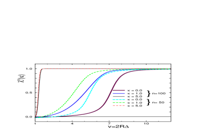
FIG. 2.: Correlation strength $\lambda^{(n)}(\kappa)$ as a function of the dimensionless phase-space volume $v=2R\Delta/\hbar$. Results are shown for two fixed multiplicity values ($n=50$ (solid) and 100 (dashed)) and for three values of the reduced pair momentum $\kappa=K/\Delta=0,\,1$, and 5 (from right to left).

Closer inspection of Eq. (135) for the Poisson multiplicity distribution shows that it is not really the phase-space volume factor $v$, but the average phase-space density

$$d={\langle n\rangle\over v^{3}}$$ (140)

which controls the strength of multi-boson effects. For a source of minimal phase-space volume $v{=}1$, the correlation strength $\lambda$ approaches zero as $\langle n\rangle{\to}\infty$ (large phase-space density $d\to\infty$); this agrees with the expectation of strong multi-boson effects in this limit. On the other hand, in the opposite limit $\langle n\rangle\to 0$ (small phase-space density $d\to 0$) $\lambda$ approaches unity, the same value as for sources with large phase-space volumes $v\to\infty$. For strong multi-boson effects to arise, it is thus not sufficient that the phase-space volume factor $v$ is small, but the phase-space density $d=\langle n\rangle/v^{3}$ must be large.

Let us now discuss some numerical results. In Figures 2 and 3 we show the correlation strength $\lambda$ as a function of the phase-space volume factor $v=2R\Delta/\hbar$. Whereas, according to Eqs. (V C) and (139), the correlation strength is independent of the scaled pair momentum $\kappa$ in the limits $v{\to}\infty$ and $v{\to}1$, Figure 2 shows that in the intermediate range $1<v<\infty$ the correlation strength $\lambda^{(n)}$ develops a $\kappa$-dependence. At fixed phase-space volume $v$, the effective strength of the correlations diminishes for smaller $\kappa$ and/or larger multiplicity $n$.

The dependence of the correlation strength on the multiplicity distribution is shown in Figure 3. For fixed $\kappa=0.3$ and constant mean multiplicity $\langle n\rangle=18$, Fig. 3 gives $\lambda$ as a function of $v$ for four different multiplicity distributions. One sees that for different multiplicity distributions the residual correlations manifest themselves quite differently. There is no universal scaling with the average phase-space density $d$ defined above; however, for typical momenta $\kappa\simeq 1$, significant residual correlation effects (i.e. noticeable deviations of $\lambda$ from its asymptotic value $\lim_{v\to\infty}\lambda{=}1$) are seen for phase-space densities above 0.2–0.3 particles per unit phase-space volume, $d\gtrsim 0.2-0.3$. At lower momenta $\kappa<1$ similarly strong effects arise from even smaller values of $d$, whereas only very high phase-space densities lead to strong multi-boson effects at large pair momenta $\kappa\gg 1$. These conclusions agree with those of Lednicky et al. [13].

FIG. 3.: Correlation strength $\lambda(\kappa)$ as a function of the dimensionless phase-space volume $v=2R\Delta/\hbar$, for fixed pair momentum $\kappa$=0.3. Results are shown for four different pion multiplicity distributions (Poisson, Bose-Einstein, Gamma distribution with $k$=8, and negative binomial (NB) distribution with $k$=6). In all cases we fixed $\langle n\rangle$=18.

Note that the multiplicity distributions studied in Fig. 3 refer to the observed pion multiplicity, after full inclusion of multi-boson effects; the measured multiplicity distribution is kept fixed while varying the phase-space density. The presentation in Fig. 3 differs from the discussion of the “Poisson limit” in Sec. III C where the input distribution was fixed to be Poissonian, and the measured multiplicity distribution $\bar{p}_{n}(v)$ of Eq. (54) then depended on $v$. The distribution $\bar{p}_{n}(v)$ corresponds to a constant correlation strength $\lambda{=}1$ and would in Fig. 3 interpolate as a constant horizontal line between the Poisson distribution at $v{\to}\infty$ and the Bose-Einstein distribution at $v{\to}1$. This must be taken into account when comparing with results from the “Poisson limit” like those discussed in [7, 10, 13].

D HBT radii

The information on the space-time structure of the source is contained in the Bose-Einstein correlation function $R_{2}({\mathchoice{{\hbox{\boldmath$\displaystyle q$}}}{{\hbox{\boldmath$\textstyle q$}}}{{\hbox{\boldmath$\scriptstyle q$}}}{{\hbox{\boldmath$\scriptscriptstyle q$}}}},{\mathchoice{{\hbox{\boldmath$\displaystyle K$}}}{{\hbox{\boldmath$\textstyle K$}}}{{\hbox{\boldmath$\scriptstyle K$}}}{{\hbox{\boldmath$\scriptscriptstyle K$}}}})$ of (101). The discussion of the “Poisson limit” in Sec. III C (cf. Eq. (64)) showed that this information is “contaminated”: the two-particle exchange term $\sum h_{i{+}j}\,G_{i}({\mathchoice{{\hbox{\boldmath$\displaystyle p$}}}{{\hbox{\boldmath$\textstyle p$}}}{{\hbox{\boldmath$\scriptstyle p$}}}{{\hbox{\boldmath$\scriptscriptstyle p$}}}}_{1},{\mathchoice{{\hbox{\boldmath$\displaystyle p$}}}{{\hbox{\boldmath$\textstyle p$}}}{{\hbox{\boldmath$\scriptstyle p$}}}{{\hbox{\boldmath$\scriptscriptstyle p$}}}}_{2})\,G_{j}({\mathchoice{{\hbox{\boldmath$\displaystyle p$}}}{{\hbox{\boldmath$\textstyle p$}}}{{\hbox{\boldmath$\scriptstyle p$}}}{{\hbox{\boldmath$\scriptscriptstyle p$}}}}_{2},{\mathchoice{{\hbox{\boldmath$\displaystyle p$}}}{{\hbox{\boldmath$\textstyle p$}}}{{\hbox{\boldmath$\scriptstyle p$}}}{{\hbox{\boldmath$\scriptscriptstyle p$}}}}_{1})$ is normalized by the corresponding “direct term” evaluated at the observed momenta ${\mathchoice{{\hbox{\boldmath$\displaystyle p$}}}{{\hbox{\boldmath$\textstyle p$}}}{{\hbox{\boldmath$\scriptstyle p$}}}{{\hbox{\boldmath$\scriptscriptstyle p$}}}}_{1},{\mathchoice{{\hbox{\boldmath$\displaystyle p$}}}{{\hbox{\boldmath$\textstyle p$}}}{{\hbox{\boldmath$\scriptstyle p$}}}{{\hbox{\boldmath$\scriptscriptstyle p$}}}}_{2}$ (i.e. by $\sum h_{i{+}j}\,G_{i}({\mathchoice{{\hbox{\boldmath$\displaystyle p$}}}{{\hbox{\boldmath$\textstyle p$}}}{{\hbox{\boldmath$\scriptstyle p$}}}{{\hbox{\boldmath$\scriptscriptstyle p$}}}}_{1},{\mathchoice{{\hbox{\boldmath$\displaystyle p$}}}{{\hbox{\boldmath$\textstyle p$}}}{{\hbox{\boldmath$\scriptstyle p$}}}{{\hbox{\boldmath$\scriptscriptstyle p$}}}}_{1})\,G_{j}({\mathchoice{{\hbox{\boldmath$\displaystyle p$}}}{{\hbox{\boldmath$\textstyle p$}}}{{\hbox{\boldmath$\scriptstyle p$}}}{{\hbox{\boldmath$\scriptscriptstyle p$}}}}_{2},{\mathchoice{{\hbox{\boldmath$\displaystyle p$}}}{{\hbox{\boldmath$\textstyle p$}}}{{\hbox{\boldmath$\scriptstyle p$}}}{{\hbox{\boldmath$\scriptscriptstyle p$}}}}_{2})$) instead of the same expression evaluated at the average momentum $\textstyle K$ (i.e. $\sum h_{i{+}j}\,G_{i}({\mathchoice{{\hbox{\boldmath$\displaystyle K$}}}{{\hbox{\boldmath$\textstyle K$}}}{{\hbox{\boldmath$\scriptstyle K$}}}{{\hbox{\boldmath$\scriptscriptstyle K$}}}},{\mathchoice{{\hbox{\boldmath$\displaystyle K$}}}{{\hbox{\boldmath$\textstyle K$}}}{{\hbox{\boldmath$\scriptstyle K$}}}{{\hbox{\boldmath$\scriptscriptstyle K$}}}})\,G_{j}({\mathchoice{{\hbox{\boldmath$\displaystyle K$}}}{{\hbox{\boldmath$\textstyle K$}}}{{\hbox{\boldmath$\scriptstyle K$}}}{{\hbox{\boldmath$\scriptscriptstyle K$}}}},{\mathchoice{{\hbox{\boldmath$\displaystyle K$}}}{{\hbox{\boldmath$\textstyle K$}}}{{\hbox{\boldmath$\scriptstyle K$}}}{{\hbox{\boldmath$\scriptscriptstyle K$}}}})$). Only in the latter case would $R_{2}({\mathchoice{{\hbox{\boldmath$\displaystyle q$}}}{{\hbox{\boldmath$\textstyle q$}}}{{\hbox{\boldmath$\scriptstyle q$}}}{{\hbox{\boldmath$\scriptscriptstyle q$}}}},{\mathchoice{{\hbox{\boldmath$\displaystyle K$}}}{{\hbox{\boldmath$\textstyle K$}}}{{\hbox{\boldmath$\scriptstyle K$}}}{{\hbox{\boldmath$\scriptscriptstyle K$}}}})$ allow for a “clean” extraction of the space-time structure of the source. For heavy-ion collisions where the sources are large it is known [42, 43] that (at least in the “Poisson limit”) these contamination effects from inadequate normalization are negligible. For small sources, like those created in $e^{+}e^{-}$ collisions, they may, however, seriously affect the extraction of the source radius.

In the “Poisson limit” Eq. (64) shows that this type of contamination can be avoided by first extracting from $R_{2}$ a (directly measurable) ratio of single particle spectra. For a dilute Gaussian source of the type (70) (i.e. in the limit $v\to\infty$) this ratio is given by

$${[N_{1}({\mathchoice{{\hbox{\boldmath$\displaystyle K$}}}{{\hbox{\boldmath$\textstyle K$}}}{{\hbox{\boldmath$\scriptstyle K$}}}{{\hbox{\boldmath$\scriptscriptstyle K$}}}})]^{2}\over N_{1}({\mathchoice{{\hbox{\boldmath$\displaystyle p$}}}{{\hbox{\boldmath$\textstyle p$}}}{{\hbox{\boldmath$\scriptstyle p$}}}{{\hbox{\boldmath$\scriptscriptstyle p$}}}}_{1})N_{1}({\mathchoice{{\hbox{\boldmath$\displaystyle p$}}}{{\hbox{\boldmath$\textstyle p$}}}{{\hbox{\boldmath$\scriptstyle p$}}}{{\hbox{\boldmath$\scriptscriptstyle p$}}}}_{2})}=\exp\left({q^{2}\,\over 4\Delta^{2}}\right)=\exp\left({\tilde{q}^{2}\over v^{2}}\right)\,.$$ (141)

For arbitrary multiplicity distributions the residual correlations prohibit such a simple procedure (the denominator of $R_{2}$ cannot in general be written as a product of single particle spectra), and the contamination of the space-time information about the source cannot be avoided. The results presented in this subsection allow, however, to estimate the relative magnitude of this contamination effect.

As usual, we parametrize the correlation function $R_{2}({\mathchoice{{\hbox{\boldmath$\displaystyle q$}}}{{\hbox{\boldmath$\textstyle q$}}}{{\hbox{\boldmath$\scriptstyle q$}}}{{\hbox{\boldmath$\scriptscriptstyle q$}}}},{\mathchoice{{\hbox{\boldmath$\displaystyle K$}}}{{\hbox{\boldmath$\textstyle K$}}}{{\hbox{\boldmath$\scriptstyle K$}}}{{\hbox{\boldmath$\scriptscriptstyle K$}}}})$ by a Gaussian in $\textstyle q$ with $\textstyle K$-dependent width parameters (HBT radii). The spherical symmetry of the Gaussian source (70) ensures that the HBT radii depend only on the modulus $\kappa$ of the scaled pair momentum (see Appendix C). However, since the denominator of $R_{2}$ involves the two measured momenta ${\mathchoice{{\hbox{\boldmath$\displaystyle p$}}}{{\hbox{\boldmath$\textstyle p$}}}{{\hbox{\boldmath$\scriptstyle p$}}}{{\hbox{\boldmath$\scriptscriptstyle p$}}}}_{1}$ and ${\mathchoice{{\hbox{\boldmath$\displaystyle p$}}}{{\hbox{\boldmath$\textstyle p$}}}{{\hbox{\boldmath$\scriptstyle p$}}}{{\hbox{\boldmath$\scriptscriptstyle p$}}}}_{2}$ (see (101) and (B8)), the correlation function $R_{2}$ depends separately on the components $q_{\parallel}$ and $q_{\perp}$ of $\textstyle q$ which are parallel and orthogonal to $\textstyle K$. This is an artifact of the above-mentioned “contamination effect”; the difference of the width parameters in the $q_{\parallel}$ and $q_{\perp}$ directions thus is a quantitative measure for this undesired contamination.

We thus write

$$R_{2}({\mathchoice{{\hbox{\boldmath$\displaystyle q$}}}{{\hbox{\boldmath$\textstyle q$}}}{{\hbox{\boldmath$\scriptstyle q$}}}{{\hbox{\boldmath$\scriptscriptstyle q$}}}},{\mathchoice{{\hbox{\boldmath$\displaystyle K$}}}{{\hbox{\boldmath$\textstyle K$}}}{{\hbox{\boldmath$\scriptstyle K$}}}{{\hbox{\boldmath$\scriptscriptstyle K$}}}})=\exp\left[-q_{\perp}^{2}\,R_{\perp}^{2}(K)-q_{\parallel}^{2}\,R_{\parallel}^{2}(K)\right]\,,$$ (142)

$$q_{\perp}=q\,\sin\theta\,,\quad q_{\parallel}=q\,\cos\theta\,,\quad\theta=\angle({\mathchoice{{\hbox{\boldmath$\displaystyle q$}}}{{\hbox{\boldmath$\textstyle q$}}}{{\hbox{\boldmath$\scriptstyle q$}}}{{\hbox{\boldmath$\scriptscriptstyle q$}}}},{\mathchoice{{\hbox{\boldmath$\displaystyle K$}}}{{\hbox{\boldmath$\textstyle K$}}}{{\hbox{\boldmath$\scriptstyle K$}}}{{\hbox{\boldmath$\scriptscriptstyle K$}}}})\,.$$ (143)

The HBT radii are then obtained by separating the constant and $\theta$-dependent terms in

$$-{d\over dq^{2}}\,R_{2}({\mathchoice{{\hbox{\boldmath$\displaystyle q$}}}{{\hbox{\boldmath$\textstyle q$}}}{{\hbox{\boldmath$\scriptstyle q$}}}{{\hbox{\boldmath$\scriptscriptstyle q$}}}},{\mathchoice{{\hbox{\boldmath$\displaystyle K$}}}{{\hbox{\boldmath$\textstyle K$}}}{{\hbox{\boldmath$\scriptstyle K$}}}{{\hbox{\boldmath$\scriptscriptstyle K$}}}})\bigg{|}_{q{=}0} = R_{\perp}^{2}(K)$$ (145)

$$+\cos^{2}\theta\left(R_{\parallel}^{2}(K)-R_{\perp}^{2}(K)\right)\,.$$

The corresponding explicit expressions are given in Appendix C, Eqs. (C1) and (C2). Before proceeding further it is useful to establish a baseline in the absence of multi-boson effects, by keeping in (C1) and (C2) only the lowest order terms $i{=}j{=}1$. Denoting these reference values by a tilde we find

$$\tilde{R}_{\perp}^{2}=\tilde{R}_{\parallel}^{2}=R^{2}\left(1-{1\over v^{2}}\right)$$ (146)

independent of the pair momentum $\kappa$. The HBT radii are seen to be smaller than the Gaussian input radius $R$ by a correction $\sim 1/v^{2}$; this is the “contamination” from the ratio (141) of single particle spectra mentioned above. In the following we will discuss multi-boson effects on the HBT radii (including additional multi-boson-induced “contamination” effects) as deviations from the baseline (146). To this end we define the dimensionless ratios

$$r_{1}={R_{\perp}^{2}\over R^{2}\left(1-{1\over v^{2}}\right)}\,,\quad r_{2}={R_{\parallel}^{2}-R_{\perp}^{2}\over R^{2}}\,.$$ (147)

Like the HBT radii themselves, these ratios depend on $v$, $\kappa$ and $\langle n\rangle$ via multi-boson symmetrization effects; in the absence of such effects (in particular in the limit $v\to\infty$) they approach $r_{1}=1$ and $r_{2}=0$. In particular, $r_{2}$ provides a relative measure for multi-boson-induced spectral contamination effects.

FIG. 4.: The ratios $r_{1}$ (thick lines) and $r_{2}$ (thin lines) as functions of $v=2R\Delta/\hbar$, for fixed multiplicity $n=20$ and for three values of the scaled pair momentum $\kappa=0,1,5$. $r_{2}$ vanishes identically for $\kappa=0$ (see Eq. (C2)).

Analytic expressions for $r_{1}$ and $r_{2}$ in the quantum saturation limit $v\to 1$ (in which the pions in the source all occupy the same quantum state and form a Bose condensate) are given in Eqs. (C). Note that in this limit both $R_{\perp}$ and $R_{\parallel}$ vanish even in the absence of multi-boson effects, due to the factor $(1-{1\over v^{2}})$ in (146). This leads to a flat Bose-Einstein correlation function $1+R_{2}$. In [7] this flatness of the correlation function was incorrectly attributed to the onset of phase coherence, resulting in an absence of Bose-Einstein correlations at low values of $q$. Lednicky et al. [13] clarified this error by pointing out that even in this limit the Bose-Einstein correlations are still present (the exchange term $R_{2}=1$ is as large as the direct term), and that the misunderstanding in [7] resulted from an incomplete analysis of the normalization of the correlation function in the Bose-Einstein condensation limit. The latter was also discussed in [10].

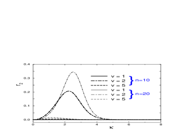
FIG. 5.: Top: The ratio $r_{1}$ as a function of the scaled pair momentum $\kappa$, for two fixed multiplicities ($n=10$ (thick lines) and $n=20$ (thin lines)) and three values for the phase-space volume factor $v=1,2,5$. For $v=1$, $r_{1}$ is independent of $\kappa$ and less than 1; but for $v=1+\epsilon$, $r_{1}$ will eventually again approach 1 at $\kappa\to\infty$. Bottom: The same for the ratio $r_{2}$; it vanishes for $v=1$.

Eqs. (C) show that for all considered multiplicity distributions $\lim_{v\to 1}r_{1}\leq 1$. The numerical results below show that the same holds true for all values of $v$. In other words, multi-boson effects always reduce the HBT radii: $R_{\perp}^{2}\leq R^{2}(1-{1\over v^{2}})$. For $v>1$ this is largely the consequence of Bose-clustering in the source ($R_{n}^{2}=a_{n}R^{2}\leq R$, see (71)) and confirms similar findings in many earlier papers. However, for $v=1$ the source is already as small as allowed by the uncertainty relation and thus cannot be compressed any further by Bose-clustering. In this case a reduced value $r_{1}<1$ must be blamed entirely on multi-boson contributions to the spectral contamination effect from the product of single particle spectra in the denominator of the Bose-Einstein correlator $R_{2}$. Eqs. (C) show that these contributions disappear for vanishing phase-space density $d=\langle n\rangle/v^{3}\to 0$, even in the limit $v\to 1$:

$$\lim_{\langle n\rangle\to 0}\lim_{v\to 1}r_{1}=1\,.$$ (148)

(For fixed multiplicity the lowest allowed value is $n=2$ for which $r_{1}$ satisfies the same rule.) However, for large phase-space densities $d\to\infty$ they are large and the ratio $r_{1}$ vanishes:

$$\lim_{\langle n\rangle\to\infty}\lim_{v\to 1}r_{1}=\lim_{\langle n\rangle\to\infty}\lim_{v\to 1}{R_{\perp}^{2}\over R^{2}\left(1-{1\over v^{2}}\right)}=0\,.$$ (149)

FIG. 6.: Top: The ratio $r_{1}$ as a function of $v$, for vanishing pair momentum and fixed average multiplicity $\langle n\rangle=20$, for four different multiplicity distributions. Bottom: The same for the ratio $r_{2}$, but for $\kappa{=}1$ (since $r_{2}{=}0$ for $\kappa{=}0$).

These last results can be generalized to arbitrary values of $v$ by rephrasing them in terms of $d$:

$$\lim_{d\to 0}r_{1} = 1\,,$$ (151)

$$\lim_{d\to 0}r_{2} = 0\,,$$ (152)

$$\lim_{d\to\infty}r_{1} = \lim_{d\to\infty}r_{2}=0\,.$$ (153)

For the limit $d\to\infty$ the proof relies on the fact that, at fixed $v$, this requires $\langle n\rangle\to\infty$; therefore only the asymptotic behavior of (71) for large $n$ is needed, in particular

$$\lim_{n\to\infty}a_{n}={1\over v}\,.$$ (154)

(Incidentally, this implies $\lim_{n\to\infty}R_{n}\Delta_{n}={R\Delta\over v}={1\over 2}$: in the limit $n\to\infty$ the effective source corresponding to $G_{n}({\mathchoice{{\hbox{\boldmath$\displaystyle p$}}}{{\hbox{\boldmath$\textstyle p$}}}{{\hbox{\boldmath$\scriptstyle p$}}}{{\hbox{\boldmath$\scriptscriptstyle p$}}}}_{1},{\mathchoice{{\hbox{\boldmath$\displaystyle p$}}}{{\hbox{\boldmath$\textstyle p$}}}{{\hbox{\boldmath$\scriptstyle p$}}}{{\hbox{\boldmath$\scriptscriptstyle p$}}}}_{2})$ saturates the uncertainty relation.) Equations (153) then follow easily from (C1) and (C2).

Figures 4–7 show numerical results for $r_{1}$ and $r_{2}$ for a variety of multiplicity distributions as functions of the phase-space volume factor $v$ and the scaled pair momentum $\kappa$. In Figures 4 and 5 we study events with fixed multiplicity ($n=10$ and $n=20$). Multi-boson symmetrization effects on the HBT radius $R_{\perp}$ and their contributions to the difference $R_{\parallel}^{2}-R_{\perp}^{2}$ (which is entirely due to the above-mentioned “spectral contamination effect”) are seen to increase as the phase-space density $d$ increases and the scaled pair momentum $\kappa$ decreases. On the other hand, Fig. 5 shows that for large pair momenta $\kappa$ the multi-boson effects vanish, irrespective of the value of $v$. As noted in [13] this reflects the exponential decrease of the momentum-space density $\sim\exp(-\kappa^{2}/2)$ at large particle momenta. This also explains why increasing $\kappa$ compresses the curves in Fig. 4 to the left.

FIG. 7.: Top: The ratio $r_{1}$ as a function of $\kappa$, for a fixed phase-space volume factor $v=5$ and fixed average multiplicity $\langle n\rangle=20$, for four different multiplicity distributions. Bottom: The same for the ratio $r_{2}$.

Note that the multi-boson effects set in rather suddenly. (As discussed in Appendix C, the vanishing of $r_{2}$ in the limits $v\to 1$ and/or $\kappa\to 0$ is due to its definition and does not imply the disappearance of multi-boson effects in these limits.) Unfortunately, we have not been able to find a simple scaling law for the threshold at which multi-boson effects on the HBT radii set in and which properly describes the observed qualitative trends.

In Figures 6 and 7 we study the dependence of multi-boson symmetrization effects on the measured pion multiplicity distribution. While the dependences on $v$ (Fig. 6) and on $\kappa$ (Fig. 7) are qualitatively similar to the case of fixed multiplicity, on a quantitative level one observes quite significant variations for different multiplicity distributions at fixed mean multiplicity $\langle n\rangle$. This demonstrates that there is no simple scaling of multi-boson effects with the average phase-space density $d=\langle n\rangle/v^{3}$. Of the four distributions considered here, the Bose-Einstein multiplicity distribution gives by far the strongest multi-particle symmetrization effects on the HBT radii: it is less effective in suppressing high-multiplicity contributions than the other considered distributions.

E The range of the residual correlations

Looking at Figure 1 and Appendix B one sees that the residual correlation $C_{2}^{({\rm res})}({\mathchoice{{\hbox{\boldmath$\displaystyle q$}}}{{\hbox{\boldmath$\textstyle q$}}}{{\hbox{\boldmath$\scriptstyle q$}}}{{\hbox{\boldmath$\scriptscriptstyle q$}}}},{\mathchoice{{\hbox{\boldmath$\displaystyle K$}}}{{\hbox{\boldmath$\textstyle K$}}}{{\hbox{\boldmath$\scriptstyle K$}}}{{\hbox{\boldmath$\scriptscriptstyle K$}}}})$ can also be parametrized by a Gaussian:

$$C_{2}^{({\rm res})}({\mathchoice{{\hbox{\boldmath$\displaystyle q$}}}{{\hbox{\boldmath$\textstyle q$}}}{{\hbox{\boldmath$\scriptstyle q$}}}{{\hbox{\boldmath$\scriptscriptstyle q$}}}},{\mathchoice{{\hbox{\boldmath$\displaystyle K$}}}{{\hbox{\boldmath$\textstyle K$}}}{{\hbox{\boldmath$\scriptstyle K$}}}{{\hbox{\boldmath$\scriptscriptstyle K$}}}})={\cal N}\left[1+{\textstyle{\lambda(\kappa){-}1\over 2}}\,e^{-q_{\perp}^{2}\,r_{\perp}^{2}(\kappa)-q_{\parallel}^{2}\,r_{\parallel}^{2}(\kappa)}\right].$$ (155)

The two newly introduced radius parameters $r_{\perp}(\kappa)$, $r_{\parallel}(\kappa)$ can be interpreted as the “range” of the residual correlations in coordinate space. A Gaussian parametrization of the full correlation function $C_{2}({\mathchoice{{\hbox{\boldmath$\displaystyle q$}}}{{\hbox{\boldmath$\textstyle q$}}}{{\hbox{\boldmath$\scriptstyle q$}}}{{\hbox{\boldmath$\scriptscriptstyle q$}}}},{\mathchoice{{\hbox{\boldmath$\displaystyle K$}}}{{\hbox{\boldmath$\textstyle K$}}}{{\hbox{\boldmath$\scriptstyle K$}}}{{\hbox{\boldmath$\scriptscriptstyle K$}}}})$ in (101) is obtained by combining (155) with (142).

From the ansatz (155) one obtains the “residual correlation radii” by separating the constant and $\theta$-dependent terms in

$${r_{\perp}^{2}(\kappa)\over R^{2}}+\cos^{2}\theta{r_{\parallel}^{2}(\kappa)-r_{\perp}^{2}(\kappa)\over R^{2}}$$ (156)

$$={B(\kappa)\,\over{\cal N}\,B(\kappa)-A(\kappa)}\,{d\over d\tilde{q}^{2}}\,C_{2}^{({\rm res})}(\tilde{\mathchoice{{\hbox{\boldmath$\displaystyle q$}}}{{\hbox{\boldmath$\textstyle q$}}}{{\hbox{\boldmath$\scriptstyle q$}}}{{\hbox{\boldmath$\scriptscriptstyle q$}}}},\mathchoice{{\hbox{\boldmath$\displaystyle\kappa$}}}{{\hbox{\boldmath$\textstyle\kappa$}}}{{\hbox{\boldmath$\scriptstyle\kappa$}}}{{\hbox{\boldmath$\scriptscriptstyle\kappa$}}})\bigg{|}_{\tilde{q}{=}0}\,,$$ (157)

where we used (120) and (133) to rewrite the coefficient in front of the $\tilde{q}^{2}$-derivative. The explicit expressions are given in Appendix C, Eqs. (C10)–(C24). Using the asymptotic expressions (B15) we find from (C10) and (C12)

$$\lim_{v\to\infty}r_{\perp}^{2}(\kappa)=\lim_{v\to\infty}r_{\parallel}^{2}(\kappa)=0\,;$$ (158)

for dilute sources the residual correlations disappear, as expected. In the opposite limit $v\to 1$ the two “residual correlation radii” are nonzero, but again equal to each other:

$$\lim_{v\to 1}\bigl{(}r_{\perp}^{2}(\kappa)-r_{\parallel}^{2}(\kappa)\bigr{)}=0\,.$$ (159)

What matters in practice is the ratio of the “residual correlation radii” to the HBT radii, $r_{\perp}/R_{\perp}$. For fixed multiplicity $n$, this ratio can be calculated analytically in the limit $v\to 1$:

$$\lim_{v\to 1}{r_{\perp}^{2}(\kappa)\over R_{\perp}^{2}(\kappa)}={1\over 4}\,{n-1\over n+1}\quad({\rm fixed}\ n).$$ (160)

For $n\to\infty$ this approaches the value ${1\over 4}$ from below; for intermediate values $1<v<\infty$ the ratio is between 0 and ${1\over 4}$. The same is true for the Poisson multiplicity distribution for which (C24) gives in the limit of large $\langle n\rangle$

$$\lim_{v\to 1}{r_{\perp}^{2}(\kappa)\over R_{\perp}^{2}(\kappa)}={1\over 4}\,{\langle n\rangle-2\over\langle n\rangle-1}+{\cal O}\bigl{(}e^{-\langle n\rangle}\bigr{)}\quad({\rm Poisson}).$$ (161)

From these analytical results it seems that the “range” of the residual correlations in coordinate space is always less than half the effective source size as measured by the HBT radii. Below we confirm this numerically. Thus, with two well-separated length scales involved, strong multi-boson effects should be clearly recognizable in the 2-particle correlation function, as exemplified in Fig. 1.

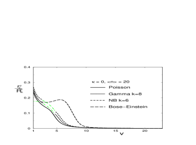
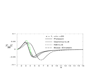
FIG. 8.: Top: $v$-dependence of the ratio $r_{\perp}^{2}/R_{\perp}^{2}$ at vanishing pair momentum $\kappa{\,=\,}0$, for a variety of multiplicity distributions, keeping the average multiplicity fixed at $\langle n\rangle{\,=\,}20$. Bottom: The same for $(r_{\parallel}^{2}-r_{\perp}^{2})/R^{2}$ at $\kappa{\,=\,}1$. The grey dashed lines indicate an interpolation as described in the text.

In Fig. 8 we show the ratios $r_{\perp}^{2}/R_{\perp}^{2}$ and $(r_{\parallel}^{2}-r_{\perp}^{2})/R^{2}$ as functions of $v$, for the same values of $\kappa$ and $\langle n\rangle$ as in Fig. 6. One sees that indeed always $r_{\perp}\lesssim{\textstyle{1\over 2}}R_{\perp}$, and that the ratio of these two parameters is largest at small values of $v$. The ratio $(r_{\parallel}^{2}-r_{\perp}^{2})/R^{2}$ alternates sign, but its absolute value always stays below about 5% and also below the ratio $r_{2}$ of (147) (see Fig. 6).

We note that the range parameters $r_{\perp}^{2}(\kappa)$ and $r_{\parallel}^{2}(\kappa)$ become ill-defined when the correlation strength $\lambda(\kappa)$ passes through 1 (see Eq. (155) and Fig. 3). We checked that at this point the function $C_{2}^{\rm res}({\mathchoice{{\hbox{\boldmath$\displaystyle q$}}}{{\hbox{\boldmath$\textstyle q$}}}{{\hbox{\boldmath$\scriptstyle q$}}}{{\hbox{\boldmath$\scriptscriptstyle q$}}}})$ is approximately, but not quite exactly constant. The remaining, albeit very weak $\textstyle q$-dependence cannot be properly absorbed by the Ansatz (155), resulting in a divergence of the expression (156). Since this is an artefact of the Ansatz (155) and does not reflect any really singular behaviour of the residual correlations, we smoothed this singularity in Fig. 8 by interpolating by hand (grey dashed lines) across the point $\lambda(\kappa){\,=\,}1$.

VI Experimental consequences

Figure 1 shows that, for fixed $n$, the residual correlations reduce the correlation function while the Bose-Einstein correlations increase it. The interplay of these effects leads to a minimum of the correlation function at intermediate values of $q$. This is different from Coulomb or strong final state interactions (FSI) which are concentrated much more strongly near $q=0$ (and which in practice one can correct for [22]). A minimum at nonzero $q$, after FSI correction, thus points to the presence of residual correlations arising from multi-boson symmetrization effects. In the limit $v\to\infty$, i.e. for vanishing phase-space density of the source, the residual correlations disappear, and so does the minimum in the correlation function. The minimum also disappears in the opposite limit, $v\to 1$, but for a different reason: in this limit the HBT-radii go to zero, and the whole correlation function becomes entirely flat.

For multiplicity-selected event samples (as they are routinely collected in heavy ion collisions because multiplicity serves as a measure for collision centrality) the absence of a minimum in the correlation function, combined with a clear positive HBT signal at $q=0$, can thus be taken as evidence against strong multi-boson symmetrization effects and provides a lower limit on the phase-space volume (upper limit on the phase-space density) of the source. The significance of this limit is controlled by the statistical error on the correlation function. The conspicuous absence of a minimum in the correlation data known to us supports the evidence for low freeze-out phase-space densities (and thus weak multi-boson effects) which was obtained with other methods [16].

On the other hand, searching for such a minimum in event ensembles with approximately fixed multiplicity appears to be the most direct approach to find signatures of multi-boson symmetrization effects in heavy ion collisions, since it does not rely on model fits to the correlation function. It must be noted, however, that multiplicity-averaging tends to smear out the minimum, making it disappear, for instance, in the “Poisson limit” of Sec. III C. To obtain a clear signature thus may require a sharp selection on multiplicity. In practice the method will be limited by event-by-event fluctuations in the slope of the momentum spectra ($\Delta$) and of the freeze-out radius $R$ which both enter the phase-space volume $v$. Detailed simulations of such smearing effects go, however, beyond the scope of the present paper and will be discussed elsewhere.

Such a search for multi-boson effects via residual correlations requires a 2-Gaussian fit to the correlation function like the one obtained by combining according to Eq. (101) the expressions (142) and (155). Compared to the usually employed fit functions this doubles the number of HBT radius parameters and thus puts very high demands on event statistics. By triggering on central collision events in order to exploit azimuthal symmetry of the emission region, the number of radius parameters in the single-Gaussian fit can in general be reduced to four [22] (instead of the only two parameters required for the spherically symmetric toy sources studied here). For equal-mass collision systems, these can be further reduced to two parameters ($R_{\perp}$ and $R_{L}$, perpendicular and parallel to the beam direction) by selecting pairs with vanishing pair momentum in the center-of-mass system [22]. To describe the residual correlations then requires only two additional parameters, $r_{\perp}$ and $r_{L}$. The complexity of the resulting fit problem is then similar to the now routinely applied 3-dimensional HBT analyses in relativistic heavy-ion physics [22], which renders the proposed search practicable.

VII Conclusions

We have studied multi-boson effects on two-particle correlations for systems with a variety of multiplicity distributions. In contrast to the previously studied case of a fixed Poissonian input multiplicity distribution at $v\to\infty$, which is then at finite $v$ modified by multi-boson effects, we find that in the general case the two-particle correlation function is affected not only by Bose-Einstein correlations, which can be used to extract source size information, but also by residual correlations which depend on the pion multiplicity distribution, the average phase-space density and the pair momentum. This is true in particular for events with fixed multiplicity.

These residual correlations affect the asymptotic normalization of the correlation function at infinite relative momentum and the “correlation strength”, i.e. the ratio of the correlation function at zero and infinite relative momentum minus 1. The asymptotic normalization depends on the multiplicity distribution, in particular the mean multiplicity $\langle n\rangle$, and the phase-space volume $v^{3}$. The correlation strength depends additionally on the pair momentum $\textstyle K$. Residual correlation effects can lead to correlation strengths which are either much larger than 1 (for example for the Bose-Einstein multiplicity distribution at intermediate values of $v$) or much smaller than one and even negative (for example for fixed multiplicity in the quantum saturation limit $v\to 1$). All this happens for completely chaotic sources as those studied in the present paper and has nothing to do with partial phase coherence in the particle emission process or other quantum optical phenomena. The residual correlations arise, even in the absence of HBT correlations, from the generically different weights of pairs, triplets, quadruplets etc. of particles within a single event and from mixed events. The former enter in the numerator, the latter in the denominator of the correlation function. These different weights play a role when multi-particle symmetrization effects begin to modify the phase-space distribution of such pairs, triplets, quadruplets ets. of identical particles, i.e. for sufficiently large phase-space densities. The residual correlations vanish only accidentally for very specific multiplicity distributions, like those of the “Poisson limit” in Sec. III C or of the “covariant current formalism” in Appendix A.

The separation of residual and genuine Bose-Einstein correlations requires a fit of the correlation function with two 3-dimensional Gaussians. It thus complicates considerably the usual HBT analysis for extracting source sizes from two-particle correlation functions. Fortunately, we could show that the range of the residual correlations and of the Bose-Einstein correlations are defined by well-separated length scales such that, at least with sufficiently accurate data, the separation is possible. In practice, the demands on the statistical accuracy of the data are formidable, and in Section VI we therefore suggested to begin such studies by restricting the fits to certain kinematic regions (small momenta in the center-of-mass system in collisions between equal-mass nuclei) where only a reduced number of fit parameters is required.

We have also made a comprehensive model study of multi-boson effects on the HBT radii extracted from the Bose-Einstein part of the correlation function. In the absence of residual correlations, we showed that it is possible to isolate the source size information by first dividing out a contamination from ratios of single-particle spectra, using measured spectra. In the presence of residual interactions this is no longer possible, and the HBT radii cannot be corrected for this unwanted contamination. In Section V D we showed how to measure it within the model and saw that it becomes dangerously large for sources with high phase-space densities, i.e. when multi-boson effects become essential.

It is quite likely that the present study eventually turns out to be rather academic since Nature only allows particles to decouple from the collision region after it has had time to expand to such low phase-space densities that multi-boson symmetrization effects become negligible. Existing data analyses seem to point in that direction [15, 16]. However, until we know this for sure we should be open to the possibility of strong multi-boson symmetrization phenomena and their complicating effect on HBT interferometry. In Section VI we have suggested an essentially model-independent way to search for such effects which requires little or no prior knowledge about the source size (except for that needed to perform final state interaction corrections): it is based on the existence of the minimum in the (FSI corrected) two-particle correlation function at non-zero relative momentum $q$ in events with (approximately) fixed multiplicity. If no such minima are found, the results from the present paper can be safely shelved, and one may return with strengthened confidence to the conventional HBT formalism and source size extraction procedure based on Eq. (64).

A Relation to the covariant current formalism

The general ansatz (1), (7) for the source density matrix on which the present paper is based is formulated in terms of the unnormalized states (8). In this Section we show that the density matrix of the “covariant current ensemble” [20, 21] which instead uses normalized states can be brought into a similar form, with one important difference: in the covariant current ensemble and in the formalism used in the present paper the normalization of the density operator and the integration over the phase-space positions at which the elementary currents are centered are performed in opposite order. We discuss some relevant implications of this difference.

The covariant current formalism is based on the density operator [20, 21]

$$\tilde{\rho}=\sum_{N=1}^{\infty}P_{N}\left(\prod_{i=1}^{N}\int d\zeta_{i}\,\rho(\zeta_{i})\int{d\phi_{i}\over 2\pi}\right)|J\rangle\langle J|\,,$$ (A1)

where $|J\rangle$ is a normalized coherent state,

$$|J\rangle \equiv |J[N;\{\zeta_{i},\phi_{i}\}]\rangle$$ (A2)

$$= e^{-\bar{n}/2}\,\exp\left[i\int d{\tilde{p}}\,\tilde{J}({\mathchoice{{\hbox{\boldmath$\displaystyle p$}}}{{\hbox{\boldmath$\textstyle p$}}}{{\hbox{\boldmath$\scriptstyle p$}}}{{\hbox{\boldmath$\scriptscriptstyle p$}}}})\,\hat{a}^{+}_{p}\right]\,|0\rangle\,,$$ (A3)

with the current $\tilde{J}({\mathchoice{{\hbox{\boldmath$\displaystyle p$}}}{{\hbox{\boldmath$\textstyle p$}}}{{\hbox{\boldmath$\scriptstyle p$}}}{{\hbox{\boldmath$\scriptscriptstyle p$}}}})$ from Eq. (4) and normalization $\exp(-\bar{n}/2)$ with $\bar{n}$ given in (10). It corresponds to a specific pion multiplicity distribution $\tilde{p}_{n}$ which can be calculated by evaluating

$$\tilde{p}_{n} = {\langle n|\hat{\rho}|n\rangle\over\langle n|n\rangle}$$ (A4)

$$= \sum_{N=1}^{\infty}P_{N}\left(\prod_{i=1}^{N}\int d\zeta_{i}\,\rho(\zeta_{i})\int{d\phi_{i}\over 2\pi}\right){\ |\langle n|J\rangle|^{2}\over\bar{n}^{n}}$$ (A5)

with the states (8). Since

$$\langle n|J\rangle=e^{-\bar{n}/2}{\bar{n}^{n}\over\sqrt{n!}}\,,$$ (A6)

each coherent state itself has a Poissonian multiplicity distribution:

$${|\langle n|J\rangle|^{2}\over\langle n|n\rangle}={\bar{n}^{n}\over n!}\,e^{-\bar{n}}\,.$$ (A7)

Thus we have

$$\tilde{p}_{n}=\sum_{N=1}^{\infty}P_{N}\left(\prod_{i=1}^{N}\int d\zeta_{i}\,\rho(\zeta_{i})\int{d\phi_{i}\over 2\pi}\right){\bar{n}^{n}\over n!}\,e^{-\bar{n}}\,,$$ (A8)

where $\bar{n}$ depends on all integration variables. By summing over $n$ and using $\sum_{n}e^{-\bar{n}}(\bar{n}^{n}/n!)=1$ and the normalization of $P_{N}$ as well as (2), one easily checks that $\tilde{p}_{n}$ is normalized:

$$\sum_{n=0}^{\infty}\tilde{p}_{n}=1\,.$$ (A9)

We can decompose the coherent state projection operator in (A1) into the set (8) of unnormalized $n$-particle states $|n\rangle$:

$$|J\rangle\langle J| = \sum_{n,m=0}^{\infty}{|n\rangle\langle n|J\rangle\langle J|m\rangle\langle m|\over\langle n|n\rangle\langle m|m\rangle}$$ (A10)

$$= \sum_{n,m=0}^{\infty}{e^{-\bar{n}}\over\sqrt{n!\,m!}}|n\rangle\langle m|\,.$$ (A11)

For the calculation of the $n$-particle spectra, which always involve equal numbers of creation and annihilation operators, only the diagonal terms $n=m$ contribute. We can thus replace the density operator $\tilde{\rho}$ of the covariant current ensemble (A1) by

$$\tilde{\rho}^{\prime}=\sum_{N=1}^{\infty}P_{N}\left(\prod_{i=1}^{N}\int d\zeta_{i}\,\rho(\zeta_{i})\int{d\phi_{i}\over 2\pi}\right){e^{-\bar{n}}\over n!}|n\rangle\langle n|\,.$$ (A12)

Writing this in the form (1), namely

$$\tilde{\rho}^{\prime}=\sum_{n=0}^{\infty}\tilde{p}_{n}\,\tilde{\rho}_{n}\,,$$ (A13)

one finds for the density operator of the subspace corresponding to events with fixed particle multiplicity $n$ the expression

$$\tilde{\rho}_{n}={1\over n!\,\tilde{p}_{n}}\sum_{N=1}^{\infty}P_{N}\left(\prod_{i=1}^{N}\int d\zeta_{i}\,\rho(\zeta_{i})\int{d\phi_{i}\over 2\pi}\right)e^{-\bar{n}}\,|n\rangle\langle n|\,.$$ (A14)

When comparing this with the ansatz (7) a characteristic difference becomes apparent: the covariant current formalism involves an additional weight function $\exp(-\bar{n}[N;\{\zeta_{i},\phi_{i}\}])$ under the integral over the positions and phases of the elementary source currents $j_{0}$. This weight results from the use of normalized coherent states.

An arbitrary weight function would at this point stop further analytic progress. For the specific weight function associated with the use of normalized coherent states, however, all $n$-particle spectra can still be calculated analytically [20, 21], in fact with much less effort than for the ansatz (7). This is due to the simplifications resulting from the fact that coherent states are eigenstates of the annihilation operator. For example, the single particle spectrum is given by

$$N_{1}({\mathchoice{{\hbox{\boldmath$\displaystyle p$}}}{{\hbox{\boldmath$\textstyle p$}}}{{\hbox{\boldmath$\scriptstyle p$}}}{{\hbox{\boldmath$\scriptscriptstyle p$}}}})=E_{p}\,{\rm tr}\bigl{(}\tilde{\rho}^{\prime}\,\hat{a}^{+}_{p}\hat{a}_{p}\bigr{)}$$ (A15)

$$=E_{p}\sum_{N=1}^{\infty}P_{N}\left(\prod_{i=1}^{N}\int d\zeta_{i}\,\rho(\zeta_{i})\int{d\phi_{i}\over 2\pi}\right)|\tilde{J}({\mathchoice{{\hbox{\boldmath$\displaystyle p$}}}{{\hbox{\boldmath$\textstyle p$}}}{{\hbox{\boldmath$\scriptstyle p$}}}{{\hbox{\boldmath$\scriptscriptstyle p$}}}})|^{2}\,\langle J|J\rangle\,.$$ (A16)

We write

$$\langle J|J\rangle=1=\sum_{n=0}^{\infty}{\bar{n}^{n}\over n!}\,e^{-\bar{n}}$$ (A17)

and calculate the normalization of the single particle spectrum as

$$\int d{\tilde{p}}\,N_{1}({\mathchoice{{\hbox{\boldmath$\displaystyle p$}}}{{\hbox{\boldmath$\textstyle p$}}}{{\hbox{\boldmath$\scriptstyle p$}}}{{\hbox{\boldmath$\scriptscriptstyle p$}}}})$$ (A18)

$$=\sum_{N=1}^{\infty}P_{N}\left(\prod_{i=1}^{N}\int d\zeta_{i}\,\rho(\zeta_{i})\int{d\phi_{i}\over 2\pi}\right)\bar{n}\sum_{n=0}^{\infty}{\bar{n}^{n}\over n!}\,e^{-\bar{n}}$$ (A19)

$$=\sum_{N=1}^{\infty}P_{N}\left(\prod_{i=1}^{N}\int d\zeta_{i}\,\rho(\zeta_{i})\int{d\phi_{i}\over 2\pi}\right)\sum_{m=0}^{\infty}m\,{\bar{n}^{m}\over m!}\,e^{-\bar{n}}$$ (A20)

$$=\sum_{m=0}^{\infty}m\,\tilde{p}_{m}=\langle m\rangle\,.$$ (A21)

The single particle spectrum is thus correctly normalized to the average particle multiplicity, calculated from the multiplicity distribution $\tilde{p}_{n}$ of the covariant current ensemble. Similarly one finds that the two-particle spectrum

$$N_{2}({\mathchoice{{\hbox{\boldmath$\displaystyle p$}}}{{\hbox{\boldmath$\textstyle p$}}}{{\hbox{\boldmath$\scriptstyle p$}}}{{\hbox{\boldmath$\scriptscriptstyle p$}}}}_{1},{\mathchoice{{\hbox{\boldmath$\displaystyle p$}}}{{\hbox{\boldmath$\textstyle p$}}}{{\hbox{\boldmath$\scriptstyle p$}}}{{\hbox{\boldmath$\scriptscriptstyle p$}}}}_{2}) = E_{p_{1}}E_{p_{2}}\sum_{N=1}^{\infty}P_{N}\left(\prod_{i=1}^{N}\int d\zeta_{i}\,\rho(\zeta_{i})\int{d\phi_{i}\over 2\pi}\right)$$ (A23)

$$\times\,|\tilde{J}({\mathchoice{{\hbox{\boldmath$\displaystyle p$}}}{{\hbox{\boldmath$\textstyle p$}}}{{\hbox{\boldmath$\scriptstyle p$}}}{{\hbox{\boldmath$\scriptscriptstyle p$}}}}_{1})|^{2}\,|\tilde{J}({\mathchoice{{\hbox{\boldmath$\displaystyle p$}}}{{\hbox{\boldmath$\textstyle p$}}}{{\hbox{\boldmath$\scriptstyle p$}}}{{\hbox{\boldmath$\scriptscriptstyle p$}}}}_{2})|^{2}\,\langle J|J\rangle$$

is correctly normalized to twice the average number of pairs calculated from $\tilde{p}_{n}$:

$$\int d{\tilde{p}}_{1}\,d{\tilde{p}}_{2}\,N_{2}({\mathchoice{{\hbox{\boldmath$\displaystyle p$}}}{{\hbox{\boldmath$\textstyle p$}}}{{\hbox{\boldmath$\scriptstyle p$}}}{{\hbox{\boldmath$\scriptscriptstyle p$}}}}_{1},{\mathchoice{{\hbox{\boldmath$\displaystyle p$}}}{{\hbox{\boldmath$\textstyle p$}}}{{\hbox{\boldmath$\scriptstyle p$}}}{{\hbox{\boldmath$\scriptscriptstyle p$}}}}_{2})=\sum_{m=0}^{\infty}m(m{-}1)\,\tilde{p}_{m}=\langle m(m{-}1)\rangle\,.$$ (A24)

From the studies in [20, 21] it is known that the normalization (A18) can be alternatively written as

$$\langle m\rangle=\langle\!\langle N\rangle\!\rangle\,n_{0}\,,$$ (A25)

where $\langle\!\langle N\rangle\!\rangle$ is the average number of elementary currents and $n_{0}$ is their normalization (6). The two-particle correlation function is in the covariant current formalism given by

$$C({\mathchoice{{\hbox{\boldmath$\displaystyle q$}}}{{\hbox{\boldmath$\textstyle q$}}}{{\hbox{\boldmath$\scriptstyle q$}}}{{\hbox{\boldmath$\scriptscriptstyle q$}}}},{\mathchoice{{\hbox{\boldmath$\displaystyle K$}}}{{\hbox{\boldmath$\textstyle K$}}}{{\hbox{\boldmath$\scriptstyle K$}}}{{\hbox{\boldmath$\scriptscriptstyle K$}}}})={\langle\!\langle N(N{-}1)\rangle\!\rangle\over\langle\!\langle N\rangle\!\rangle^{2}}\left(1+{\left|\int_{x}S(x,{\mathchoice{{\hbox{\boldmath$\displaystyle K$}}}{{\hbox{\boldmath$\textstyle K$}}}{{\hbox{\boldmath$\scriptstyle K$}}}{{\hbox{\boldmath$\scriptscriptstyle K$}}}})\,e^{iq\cdot x}\right|^{2}\over\int_{x}S(x,{\mathchoice{{\hbox{\boldmath$\displaystyle p$}}}{{\hbox{\boldmath$\textstyle p$}}}{{\hbox{\boldmath$\scriptstyle p$}}}{{\hbox{\boldmath$\scriptscriptstyle p$}}}}_{1})\int_{y}S(x,{\mathchoice{{\hbox{\boldmath$\displaystyle p$}}}{{\hbox{\boldmath$\textstyle p$}}}{{\hbox{\boldmath$\scriptstyle p$}}}{{\hbox{\boldmath$\scriptscriptstyle p$}}}}_{2})}\right)$$ (A26)

where the effective emission function is nothing but the Wigner density associated with the currents $J$:

$$S(x,{\mathchoice{{\hbox{\boldmath$\displaystyle K$}}}{{\hbox{\boldmath$\textstyle K$}}}{{\hbox{\boldmath$\scriptstyle K$}}}{{\hbox{\boldmath$\scriptscriptstyle K$}}}})=\int\frac{d^{4}y}{2(2\pi)^{3}}\,e^{-iK{\cdot}y}\left\langle J^{*}(x+{\textstyle{1\over 2}}y)J(x-{\textstyle{1\over 2}}y)\right\rangle\,.$$ (A27)

This is, up to the prefactor, the standard form (64). The covariant current ensemble with its multiplicity distribution $\tilde{p}_{n}$ is thus a second example (besides the “Poisson limit” of Section III C) for a system in which multi-boson effects do not cause residual correlations. Up to the different normalization ($\langle\!\langle N(N{-}1)\rangle\!\rangle$ vs. 1), the only difference between the density operator (7) in the “Poisson limit” and the covariant current ensemble with the density operator (A12) is the different definition of the effective emission function: in the former case it is given by Eqs. (62) and (63) while for the latter the much simpler definition (A27), with all multi-boson effects already fully accounted for. The price to be paid is a more complicated expression for the multiplicity distribution ((A8) vs. (54) – while, for Gaussian sources, the latter is known analytically, the former seems to require numerical evaluation). In both cases the measured multiplicity distribution ($\bar{p}_{n}$ and $\tilde{p}_{n}$, respectively) depends in a complicated way on the mean phase-space density $d$ of the source.

B Calculating the correlation functions

In this Section we give some technical steps for the analytical evaluation of the correlation functions for the Gaussian sources defined in Sec. IV.

Let us define

$$A_{ij}(\kappa) = h_{i{+}j}\,c_{i}\,c_{j}\,e^{-{\kappa^{2}\over 2}\bigl{(}{1\over a_{i}}+{1\over a_{j}}\bigr{)}}\,,$$ (B2)

$$B_{ij}(\kappa) = h_{i}\,h_{j}\,c_{i}\,c_{j}\,e^{-{\kappa^{2}\over 2}\bigl{(}{1\over a_{i}}+{1\over a_{j}}\bigr{)}}\,,$$ (B3)

$$A(\kappa) = \sum_{i,j=1}^{\infty}A_{ij}(\kappa)\,,$$ (B4)

$$B(\kappa) = \sum_{i,j=1}^{\infty}B_{ij}(\kappa)\,,$$ (B5)

as well as

$$E_{ij}(\tilde{\mathchoice{{\hbox{\boldmath$\displaystyle q$}}}{{\hbox{\boldmath$\textstyle q$}}}{{\hbox{\boldmath$\scriptstyle q$}}}{{\hbox{\boldmath$\scriptscriptstyle q$}}}},\mathchoice{{\hbox{\boldmath$\displaystyle\kappa$}}}{{\hbox{\boldmath$\textstyle\kappa$}}}{{\hbox{\boldmath$\scriptstyle\kappa$}}}{{\hbox{\boldmath$\scriptscriptstyle\kappa$}}})=e^{-{\tilde{q}^{2}\over 2v^{2}}\bigl{(}{1\over a_{i}}{+}{1\over a_{j}}\bigr{)}}\cosh\left[{\tilde{\mathchoice{{\hbox{\boldmath$\displaystyle q$}}}{{\hbox{\boldmath$\textstyle q$}}}{{\hbox{\boldmath$\scriptstyle q$}}}{{\hbox{\boldmath$\scriptscriptstyle q$}}}}{\cdot}\mathchoice{{\hbox{\boldmath$\displaystyle\kappa$}}}{{\hbox{\boldmath$\textstyle\kappa$}}}{{\hbox{\boldmath$\scriptstyle\kappa$}}}{{\hbox{\boldmath$\scriptscriptstyle\kappa$}}}\over v}\left({1\over a_{i}}{-}{1\over a_{j}}\right)\right].$$ (B6)

A few simple steps, using eqs. (71) and (104) and exploiting the symmetry of the sums under exchange of $i$ and $j$, lead from (101) to

$$C_{2}^{({\rm res})}(\tilde{\mathchoice{{\hbox{\boldmath$\displaystyle q$}}}{{\hbox{\boldmath$\textstyle q$}}}{{\hbox{\boldmath$\scriptstyle q$}}}{{\hbox{\boldmath$\scriptscriptstyle q$}}}},\mathchoice{{\hbox{\boldmath$\displaystyle\kappa$}}}{{\hbox{\boldmath$\textstyle\kappa$}}}{{\hbox{\boldmath$\scriptstyle\kappa$}}}{{\hbox{\boldmath$\scriptscriptstyle\kappa$}}}) = {\sum_{i,j=1}^{\infty}A_{ij}(\kappa)\,E_{ij}(\tilde{\mathchoice{{\hbox{\boldmath$\displaystyle q$}}}{{\hbox{\boldmath$\textstyle q$}}}{{\hbox{\boldmath$\scriptstyle q$}}}{{\hbox{\boldmath$\scriptscriptstyle q$}}}},\mathchoice{{\hbox{\boldmath$\displaystyle\kappa$}}}{{\hbox{\boldmath$\textstyle\kappa$}}}{{\hbox{\boldmath$\scriptstyle\kappa$}}}{{\hbox{\boldmath$\scriptscriptstyle\kappa$}}})\over\sum_{i,j=1}^{\infty}B_{ij}(\kappa)\,E_{ij}(\tilde{\mathchoice{{\hbox{\boldmath$\displaystyle q$}}}{{\hbox{\boldmath$\textstyle q$}}}{{\hbox{\boldmath$\scriptstyle q$}}}{{\hbox{\boldmath$\scriptscriptstyle q$}}}},\mathchoice{{\hbox{\boldmath$\displaystyle\kappa$}}}{{\hbox{\boldmath$\textstyle\kappa$}}}{{\hbox{\boldmath$\scriptstyle\kappa$}}}{{\hbox{\boldmath$\scriptscriptstyle\kappa$}}})}\,,$$ (B7)

$$R_{2}(\tilde{\mathchoice{{\hbox{\boldmath$\displaystyle q$}}}{{\hbox{\boldmath$\textstyle q$}}}{{\hbox{\boldmath$\scriptstyle q$}}}{{\hbox{\boldmath$\scriptscriptstyle q$}}}},\mathchoice{{\hbox{\boldmath$\displaystyle\kappa$}}}{{\hbox{\boldmath$\textstyle\kappa$}}}{{\hbox{\boldmath$\scriptstyle\kappa$}}}{{\hbox{\boldmath$\scriptscriptstyle\kappa$}}}) = {\sum_{i,j=1}^{\infty}A_{ij}(\kappa)\,e^{-{\tilde{q}^{2}\over 2}(a_{i}+a_{j})}\over\sum_{i,j=1}^{\infty}A_{ij}(\kappa)\,E_{ij}(\tilde{\mathchoice{{\hbox{\boldmath$\displaystyle q$}}}{{\hbox{\boldmath$\textstyle q$}}}{{\hbox{\boldmath$\scriptstyle q$}}}{{\hbox{\boldmath$\scriptscriptstyle q$}}}},\mathchoice{{\hbox{\boldmath$\displaystyle\kappa$}}}{{\hbox{\boldmath$\textstyle\kappa$}}}{{\hbox{\boldmath$\scriptstyle\kappa$}}}{{\hbox{\boldmath$\scriptscriptstyle\kappa$}}})}\,.$$ (B8)

For very dilute ($v\to\infty$) and very dense ($v\to 1$) sources Eqs. (IV A) and (IV A) can be used to calculate analytically the behaviour of the correlation function in the limits $q\to 0$ and $q\to\infty$. Note that in these limits the dependence on the angle between $\tilde{\mathchoice{{\hbox{\boldmath$\displaystyle q$}}}{{\hbox{\boldmath$\textstyle q$}}}{{\hbox{\boldmath$\scriptstyle q$}}}{{\hbox{\boldmath$\scriptscriptstyle q$}}}}$ and $\textstyle\kappa$ (which enters via (B6)) disappears such that all following results depend only on the modulus $\kappa$ of the pair momentum:

$\textstyle 1.\ q\to\infty:$

For $v\to\infty$ the $q^{2}$-dependent exponential terms in the numerator of $R_{2}$ are much smaller than those in the denominator, and the Bose-Einstein correlations thus vanish as $q\to\infty$. For $v\to 1$ the analysis is only slightly harder: writing $v=1+\epsilon$, one finds that the exponential terms of both the numerator and denominator are given by $\exp[-\tilde{q}^{2}(1-\epsilon)]$ for all values of $i,j$ except for the lowest order term with $i=j=1$; for the latter the numerator goes as $\exp[-\tilde{q}^{2}]$ while the denominator goes as $\exp[-\tilde{q}^{2}(1-2\epsilon)]$. Again the numerator vanishes more quickly, and the Bose-Einstein correlations disappear at $q\to\infty$, as they should.

For the residual correlations (B7) one checks similarly that in both limits ($v\to\infty$ and $v\to 1$) for $q\to\infty$ numerator and denominator are both dominated by the term $i=j=1$, giving

$$\lim_{q\to\infty}C_{2}^{({\rm res})}(\tilde{\mathchoice{{\hbox{\boldmath$\displaystyle q$}}}{{\hbox{\boldmath$\textstyle q$}}}{{\hbox{\boldmath$\scriptstyle q$}}}{{\hbox{\boldmath$\scriptscriptstyle q$}}}},\mathchoice{{\hbox{\boldmath$\displaystyle\kappa$}}}{{\hbox{\boldmath$\textstyle\kappa$}}}{{\hbox{\boldmath$\scriptstyle\kappa$}}}{{\hbox{\boldmath$\scriptscriptstyle\kappa$}}})={A_{11}\over B_{11}}={h_{2}\over h_{1}^{2}}\equiv{\cal N}\,.$$ (B9)

$\textstyle 2.\ q\to 0:$

In this limit $R_{2}$ approaches trivially the value 1 (see (101)), while the residual correlations are given by

$$\lim_{q\to 0}C_{2}^{({\rm res})}(\tilde{\mathchoice{{\hbox{\boldmath$\displaystyle q$}}}{{\hbox{\boldmath$\textstyle q$}}}{{\hbox{\boldmath$\scriptstyle q$}}}{{\hbox{\boldmath$\scriptscriptstyle q$}}}},\mathchoice{{\hbox{\boldmath$\displaystyle\kappa$}}}{{\hbox{\boldmath$\textstyle\kappa$}}}{{\hbox{\boldmath$\scriptstyle\kappa$}}}{{\hbox{\boldmath$\scriptscriptstyle\kappa$}}})={A(\kappa)\over B(\kappa)}\,.$$ (B10)

The incoherence parameter defined in Eq. (67) is thus $\lambda_{\rm incoh}(\kappa)=1$, whereas the correlation strength (66) is given by (V C).

Other useful limiting expressions are

$$\lim_{v\to\infty}h_{1}=\langle n\rangle\,,$$ (B11)

$$\lim_{v\to\infty}h_{2}=\langle n(n{-}1)\rangle\,,$$ (B12)

$$\lim_{v\to\infty}h_{i}=\langle n(n{-}1)\cdots(n{-}i{+}1)\rangle\ \ {\rm for}\ i\geq 2\,,$$ (B13)

$$\lim_{v\to\infty}A(\kappa)=\lim_{v\to\infty}A_{11}(\kappa)=\langle n(n{-}1)\rangle\,e^{-\kappa^{2}}\,,$$ (B14)

$$\lim_{v\to\infty}B(\kappa)=\lim_{v\to\infty}B_{11}(\kappa)=\langle n\rangle^{2}\,e^{-\kappa^{2}}\,,$$ (B15)

and (to linear accuracy in $\epsilon$)

$$\lim_{v\to 1+\epsilon}h_{i}=\bigl{(}1+{\textstyle{3\over 2}}i\epsilon\bigr{)}\sum_{n=i}^{\infty}p_{n}-{\textstyle{3\over 2}}\epsilon p_{i}\ \ {\rm for}\ i\geq 1\,,$$ (B19)

$$\lim_{v\to 1+\epsilon}A(\kappa)={\langle n(n-1)\rangle\over 2}e^{-\kappa^{2}}$$

$$\qquad\times\left[1-(\kappa^{2}{-}3)\epsilon+{\langle n\rangle-(1{-}p_{0})\over\langle n(n{-}1)\rangle}(2\kappa^{2}{-}3)\epsilon\right]\,,$$

$$\lim_{v\to 1+\epsilon}B(\kappa)=\langle n\rangle^{2}e^{-\kappa^{2}}\left[1-{\langle n\rangle-(1{-}p_{0})\over\langle n\rangle}(\kappa^{2}{-}3)\epsilon\right]\,.$$

These last identities require the evaluation of the following sums involving $\tilde{h}_{i}\equiv\sum_{n=i}^{\infty}p_{n}$:

$$\sum_{i=2}^{\infty}\tilde{h}_{i}=\langle n\rangle-(1{-}p_{0})\,,$$ (B21)

$$\sum_{i,j=1}^{\infty}\tilde{h}_{i{+}j}={\langle n(n{-}1)\rangle\over 2}\,,$$ (B22)

$$\sum_{i,j=1}^{\infty}\tilde{h}_{i{+}j{+}1}={\langle(n{-}1)(n{-}2)\rangle\over 2}-p_{0}\,,$$ (B23)

which is achieved by appropriate reordering and relabelling of the nested sums.

C Calculating the radius parameters

Inserting (B8) into (145) and separating the constant and $\theta$-dependent terms one finds

$${R_{\perp}^{2}(\kappa)\over R^{2}}=\sum_{i,j=1}^{\infty}{A_{ij}(\kappa)\over 2\,A(\kappa)}\Bigl{[}(a_{i}{+}a_{j})-{1\over v^{2}}\Bigl{(}{1\over a_{i}}+{1\over a_{j}}\Bigr{)}\Bigr{]}\,,$$ (C1)

$${R_{\parallel}^{2}(\kappa)-R_{\perp}^{2}(\kappa)\over R^{2}}={\kappa^{2}\over v^{2}}\sum_{i,j=1}^{\infty}{A_{ij}(\kappa)\over 2\,A(\kappa)}\Bigl{(}{1\over a_{i}}-{1\over a_{j}}\Bigr{)}^{2}\,.$$ (C2)

In the dilute gas limit $v\to\infty$ only the lowest order terms $i{=}j{=}1$ contribute to the sums, and one finds the expressions (146). In the opposite limit $v\to 1$ one can use (B19)–(B19) to obtain

$$\lim_{v\to 1}r_{1} = 2{\langle n\rangle-(1{-}p_{0})\over\langle n(n-1)\rangle}$$ (C4)

$$= \left\{\begin{array}[]{ll}{2\over n}&\ \ {\rm for\ fixed}\ n\geq 2\,,\\ {1\over 1+\langle n\rangle}&\ \ {\rm Bose{-}Einstein\,,}\\ 2{\langle n\rangle-1+e^{-\langle n\rangle}\over\langle n\rangle^{2}}&\ \ {\rm Poisson\,,}\end{array}\right.$$ (C8)

$$\lim_{v\to 1}r_{2} = 0\,.$$ (C9)

All these limits are $\kappa$-independent; however, in the intermediate region $1<v<\infty$ the HBT radii develop a $\kappa$-dependence as shown by the numerical results in Sec. V D.

The vanishing of $r_{2}$ in the limit $v\to 1$ has an interesting origin: in this limit the functions $G_{i}({\mathchoice{{\hbox{\boldmath$\displaystyle p$}}}{{\hbox{\boldmath$\textstyle p$}}}{{\hbox{\boldmath$\scriptstyle p$}}}{{\hbox{\boldmath$\scriptscriptstyle p$}}}}_{1},{\mathchoice{{\hbox{\boldmath$\displaystyle p$}}}{{\hbox{\boldmath$\textstyle p$}}}{{\hbox{\boldmath$\scriptstyle p$}}}{{\hbox{\boldmath$\scriptscriptstyle p$}}}}_{2})$ in (71) become all identical, and the single particle spectrum (48) is again a simple Gaussian with width $\Delta$, just as in the opposite limit $v\to\infty$. In this case the angle-dependent term $\sim{\mathchoice{{\hbox{\boldmath$\displaystyle q$}}}{{\hbox{\boldmath$\textstyle q$}}}{{\hbox{\boldmath$\scriptstyle q$}}}{{\hbox{\boldmath$\scriptscriptstyle q$}}}}{\cdot}{\mathchoice{{\hbox{\boldmath$\displaystyle K$}}}{{\hbox{\boldmath$\textstyle K$}}}{{\hbox{\boldmath$\scriptstyle K$}}}{{\hbox{\boldmath$\scriptscriptstyle K$}}}}$ drops out from the product of single particle spectra in the denominator of the Bose-Einstein correlator $R_{2}$, and the two HBT radii $R_{\perp}$ and $R_{\parallel}$ become equal.

The “residual correlation radii” are obtained by inserting (B7) into (156) and separating the constant and $\theta$-dependent pieces:

$${r_{\perp}^{2}(\kappa)\over R^{2}}={A(\kappa)\over{\cal N}\,B(\kappa)-A(\kappa)}\,$$ (C10)

$$\quad\times{1\over 2v^{2}}\sum_{i,j=1}^{\infty}\Bigl{(}{B_{ij}(\kappa)\over B(\kappa)}-{A_{ij}(\kappa)\over A(\kappa)}\Bigr{)}\Bigl{(}{1\over a_{i}}+{1\over a_{j}}\Bigr{)}\,,$$ (C11)

$${r_{\parallel}^{2}(\kappa)-r_{\perp}^{2}(\kappa)\over R^{2}}={A(\kappa)\over{\cal N}\,B(\kappa)-A(\kappa)}$$ (C12)

$$\quad\times{\kappa^{2}\over 2v^{2}}\,\sum_{i,j=1}^{\infty}\Bigl{(}{A_{ij}(\kappa)\over A(\kappa)}-{B_{ij}(\kappa)\over B(\kappa)}\Bigr{)}\Bigl{(}{1\over a_{i}}-{1\over a_{j}}\Bigr{)}^{2}\,.$$ (C13)

To facilitate the discussion in the main text (Section V E) we here give a specific expression in the limit $v\to 1$. We decompose the r.h.s. of (C10) into three factors which we expand in powers of $\epsilon=v-1$:

$$\lim_{v\to 1+\epsilon}A(\kappa)=a_{0}+a_{1}\,\epsilon+\dots\,,$$ (C15)

$$\lim_{v\to 1+\epsilon}\bigl{(}{\cal N}\,B(\kappa)-A(\kappa)\bigr{)}=b_{0}+b_{1}\,\epsilon+\dots\,,$$ (C17)

$$\lim_{v\to 1+\epsilon}{1\over 2v^{2}}\sum_{ij}\dots=c_{0}+c_{1}\,\epsilon+\dots\,.$$

The lowest order terms have been calculated (see also (B19)):

$$a_{0} = {\langle n(n{-}1)\rangle\over 2}e^{-\kappa^{2}}\,,$$ (C19)

$$b_{0} = \left({1{-}p_{0}{-}p_{1}\over(1{-}p_{0})^{2}}\langle n\rangle^{2}-{\langle n(n{-}1)\rangle\over 2}\right)e^{-\kappa^{2}}\,,$$ (C20)

$$c_{0} = 0\,,$$ (C21)

$$c_{1} = -{1{-}p_{0}\over\langle n\rangle}+2{\langle n(n{-}1)\rangle\over 2\langle n\rangle^{2}}\,.$$ (C22)

Using Eq. (C4) in the form

$$\lim_{v\to 1+\epsilon}R_{\perp}^{2}(\kappa)=2{\langle n\rangle-(1{-}p_{0})\over\langle n(n{-}1)\rangle}\,2\,\epsilon\,R^{2}$$ (C23)

one finds

$$\lim_{v\to 1}{r_{\perp}^{2}(\kappa)\over R_{\perp}^{2}(\kappa)}={1\over 4}{\langle n(n{-}1)\rangle\over\langle n\rangle-(1{-}p_{0})}{a_{0}\,c_{1}\over b_{0}}\,.$$ (C24)

This relation is the basis of the discussion in Sec. V E.

For the Bose-Einstein multiplicity distribution (112) an unfortunate coincidence causes both $b_{0}$ and $c_{1}$ to vanish. In this case their ratio in (C24) must be replaced by $c_{2}/b_{1}$. The calculation of $c_{2}$ requires a consistent calculation to order $\epsilon^{2}$ which we have not done. Therefore, for the case of a Bose-Einstein distribution we have no analytical expression for the limit (C24).

REFERENCES

- [1] W.A. Zajc, Phys. Rev. D 35, 3396 (1987).
- [2] S. Pratt, Phys. Lett. B 301, 159 (1993); Phys. Rev. C 50, 469 (1994); S. Pratt and V. Zelevinsky, Phys. Rev. Lett. 72, 816 (1994).
- [3] W.Q. Chao, C.S. Gao, and Q.H. Zhang, J. Phys. G 21, 847 (1995); Q.H. Zhang, W.Q. Chao, and C.S. Gao, Phys. Rev. C 52, 2064 (1995).
- [4] A. Bialas and A. Krzywicki, Phys. Lett. B 354, 134 (1995); A. Bialas and K. Zalewski, Phys. Lett. B 436, 153 (1998); and Eur. Phys. J. C 6, 349 (1999).
- [5] J. Wosiek, Phys. Lett. B 399, 130 (1997); K. Fialkowski, R. Wit and J. Wosiek, Phys. Rev. D 58, 094013 (1998).
- [6] Q.H. Zhang, Phys. Lett. B 406, 366 (1997); Phys. Rev. C 57, 877 (1998); Phys. Rev. C 58, R18 (1998); and Nucl. Phys. A634, 190 (1998).
- [7] T. Csörgő and J. Zimányi, Phys. Rev. Lett. 80, 916 (1998); J. Zimányi and T. Csörgő, Heavy Ion Physics 9, 241 (1999).
- [8] U.A. Wiedemann, Phys. Rev. C 57, 3324 (1998).
- [9] R.L. Ray, Phys. Rev. C 57, 2523 (1998); R.L. Ray and G.W. Hoffmann, Phys. Rev. C 60, 014906 (1999).
- [10] Q.H. Zhang, P. Scotto, and U. Heinz, Phys. Rev. C 58, 3757 (1998).
- [11] S.V. Akkelin and Yu.M. Sinyukov, Nucl. Phys. A661, 613c (1999).
- [12] A. Bialas and K. Zalewski, Phys. Rev. C 59, 097502 (1999).
- [13] R. Lednicky et al., Phys. Rev. C 61, 034901 (2000).
- [14] G.F. Bertsch, Phys. Rev. Lett. 72, 2349 (1994).
- [15] J. Barrette et al. (E877 Coll.), Phys. Rev. Lett. 78, 2916 (1997).
- [16] D. Ferenc, U. Heinz, B. Tomášik, U.A. Wiedemann, and J.G. Cramer, Phys. Lett. B 457, 347 (1999); B. Tomášik, U. Heinz, and U.A. Wiedemann, nucl-th/9907096.
- [17] J. Rafelski and J. Letessier, nucl-th/9903018; J. Letessier, A. Tounsi, and J. Rafelski, nucl-th/9911043; J. Letessier and J. Rafelski, nucl-th/0003014.
- [18] Q.H. Zhang, Phys. Rev. C 59, 1646 (1999).
- [19] We will repeatedly use the phrase “Poissonian input multiplicity distribution”. In order to avoid confusion we stress that by this we mean that the multiplicity distribution is Poissonian in the infinite phase-space volume limit , but differs from a Poissonian at finite values of in a specific, -dependent way (see for example Eq. (54)). It does not mean that at finite one starts out with a Poissonian multiplicity distribution and that multiboson effects then change this input into something else. Multiboson symmetrization itself cannot change the multiplicity distribution, as imprecise formulations (e.g. in [7]) may have sometimes suggested: starting from exactly classical (distinguishable) particles in a given phase-space volume and then symmetrizing the multiparticle wave function still leaves us with exactly particles, not more and not less.
- [20] M. Gyulassy, S.K. Kauffmann, and L.W. Wilson, Phys. Rev. C 20, 2267 (1979).
- [21] S. Chapman and U. Heinz, Phys. Lett. B 340, 250 (1994); U. Heinz, in Correlations and Clustering Phenomena in Subatomic Physic (eds. M.N. Harakeh, J.H. Koch, and O. Scholten), NATO ASI Series B 359, 137 (1997) (Plenum, New York) (nucl-th/9609029).
- [22] U.A. Wiedemann and U. Heinz, Phys. Rep. 319, 145 (1999); U. Heinz and B.V. Jacak, Ann. Rev. Nucl. Part. Sci. 49, 529 (1999) (nucl-th/9902020).
- [23] W.A. Zajc, in Particle Production in Highly Excited Matter (eds. H.H. Gutbrod and J. Rafelski), NATO ASI Series B 303, 435 (1993) (Plenum, New York).
- [24] C. Slotta and U. Heinz, Phys. Lett. B 391, 469 (1997).
- [25] P. Scotto, PhD thesis, University of Regensburg, Sept. 1999; P. Scotto and U. Heinz, manuscript in preparation.
- [26] W.Q. Chao, C.S. Gao, and Q.H. Zhang, Phys. Rev. C 49, 3324 (1994). (In Eq. (2) of that paper the normalization factor was inadvertently omitted but the rest of the paper shows that normalized coherent states were used.)
- [27] C. Slotta, PhD thesis, University of Regensburg, Jan. 1999.
- [28] E.V. Shuryak, Phys. Lett. B 44, 387 (1973).
- [29] R.M. Weiner, Phys. Lett. B 232, 278 (1989); 242, 547 (1990); M. Plümer, L.V. Razumov, and R.M. Weiner, ibid. 286, 335 (1992); I.V. Andreev, M. Plümer, and R.M. Weiner, Int. J. Mod. Phys. A 8, 4577 (1993).
- [30] M. Biyajima, A. Bartl, T. Mizoguchi, N. Suzuki, and O. Terazawa, Prog. Theor. Phys. 84, 931 (1990); N. Suzuki and M. Biyajima, ibid. 88, 609 (1992).
- [31] J.G. Cramer, Phys. Rev. C 43, 2798 (1991); J.G. Cramer and K. Kadija, ibid. 53, 908 (1996).
- [32] U. Heinz and Q.H. Zhang, Phys. Rev. C 56, 426 (1997).
- [33] U. Heinz, in Measuring the Size of Things in the Universe: HBT Interferometry and Heavy Ion Physics (eds. S. Costa, S. Albergo, A. Insolia, and C. Tuve), p. 66 (World Scientific, Singapore, 1999) (hep-ph/9806512).
- [34] U.A. Wiedemann, D. Ferenc, and U. Heinz, Phys. Lett. B 449, 347 (1999).
- [35] H. Merlitz and D. Pelte, Phys. Lett. B 415, 411 (1997); Z. Phys. A 357, 175 (1997).
- [36] U.A. Wiedemann et al., Phys. Rev. C 56, R614 (1997).
- [37] K. Geiger, J. Ellis, U. Heinz, and U.A. Wiedemann, Phys. Rev. D 61, 054002 (2000).
- [38] The astute reader will have noticed that the spectra and correlations in the “Poisson limit” of Sec. III C do depend on . The reason is that in this case the measured multiplicity distribution given in (54) depends on via (55). However, it really depends only on the product — by rescaling the normalization of the elementary currents and the parameter in (54) simultaneously, keeping their product fixed, one can either set or . In other words, the normalization of the elementary currents does not enter any physical results directly, but only via the multiplicity distribution if the latter is allowed to explicitly depend on .
- [39] U.A. Wiedemann, J. Ellis, U. Heinz, and K. Geiger, in Ref. [33], p. 135 (nucl-th/9808043).
- [40] In [37], Eq. (38), an incorrect expression was given for which resulted from an incorrect rewriting of the correct expression given in [39]. Since the numerical simulations in [37] were compared with the original correct analytical expression, all figures in [37] are correct, although the discussion in the paragraph following Eq. (38) in [37] is inaccurate and slightly misleading.
- [41] W.A. Zajc et al., Phys. Rev. C 29, 2173 (1984).
- [42] S. Chapman, P. Scotto, and U. Heinz, Heavy Ion Physics 1, 1 (1995).
- [43] S. Pratt, Phys. Rev. C 56, 1095 (1997).