CPT-2000/P.4015

UAB-FT-487

$K^{0}$–$\bar{K^{0}}$ Mixing in the $1/N_{c}$ Expansion

Santiago Peris^a and Eduardo de Rafael^b

^a Grup de Física Teòrica and IFAE

Universitat Autònoma de Barcelona, 08193 Barcelona, Spain.

^b Centre de Physique Théorique

CNRS-Luminy, Case 907

F-13288 Marseille Cedex 9, France

We present the result for the invariant $\hat{B}_{K}$ factor of $K^{0}$–$\bar{K^{0}}$ mixing in the chiral limit and to next–to– leading order in the $1/N_{c}$ expansion. We explicitly demonstrate the cancellation of the renormalization scale and scheme dependences between short– and long–distance contributions in the final expression. Numerical estimates are then given, by taking into account increasingly refined short– and long–distance constraints of the underlying QCD Green’s function which governs the $\hat{B}_{K}$ factor.

1 Introduction

The Standard Model predicts strangeness changing transitions with $\Delta S=2$ via two virtual $W$–exchanges between quark lines, the so–called box diagrams. The low–energy physics of these transitions is governed by an effective Hamiltonian which is proportional to the local four–quark operator, (summation over colour indices within brackets is understood and $q_{L}\equiv\frac{1-\gamma_{5}}{2}q$,)

$$Q_{\Delta S=2}(x)\equiv(\bar{s}_{L}(x)\gamma^{\mu}d_{L}(x))(\bar{s}_{L}(x)\gamma_{\mu}d_{L}(x)),$$ (1.1)

modulated by a quadratic form of the flavour mixing matrix elements $\lambda_{q}=V_{\rm qd}^{\ast}V_{\rm qs}\,,\,{\rm q}={\rm u,c,t}\,,$ with coefficient functions $F_{1,2,3}$ of the heavy masses of the fields $t$, $Z^{0}$, $W^{\pm}$, $b$, and $c$ which have been integrated out :

$${{\cal H}}_{\rm eff}^{\Delta S=2}=\frac{G_{F}^{2}M_{W}^{2}}{4\pi^{2}}\left[\lambda_{c}^{2}F_{1}+\lambda_{t}^{2}F_{2}+2\lambda_{c}\lambda_{t}F_{3}\right]C_{\Delta S=2}(\mu)Q_{\Delta S=2}(x)\,.$$ (1.2)

The operator $Q_{\Delta S=2}$ is multiplicatively renormalizable and has an anomalous dimension $\gamma(\alpha_{s})$ which in perturbative QCD (pQCD) is defined by the equation

$$\mu^{2}\frac{d}{d\mu^{2}}<Q_{\Delta S=2}>=-\frac{1}{2}\gamma(\alpha_{s})<Q_{\Delta S=2}>\,,\quad\gamma(\alpha_{s})=\frac{\alpha_{\mbox{\rm{\scriptsize s}}}}{\pi}\gamma_{1}+\left(\frac{\alpha_{\mbox{\rm{\scriptsize s}}}}{\pi}\right)^{2}\gamma_{2}+\cdots\,.$$ (1.3)

with $\left(\beta_{1}=\frac{1}{6}(-11N_{c}+2n_{f})\right)$

$$\gamma_{1}=\frac{3}{2}\left(1-\frac{1}{N_{c}}\right)\quad\mbox{\rm and}\quad\gamma_{2}=\frac{1}{32}\left(1-\frac{1}{N_{c}}\right)\left[-\frac{19}{3}N_{c}+\frac{4}{3}n_{f}-21+57\frac{1}{N_{c}}+4\beta_{1}\kappa\right]\,,$$ (1.4)

where $\kappa\!=\!0$ in the naïve dimensional renormalization scheme (NDR) and $\kappa\!=\!-4$ in the ’t Hooft–Veltman renormalization scheme (HV). The renormalization $\mu$–scale dependence of the Wilson coefficient $C_{\Delta S=2}(\mu)$ in Eq. (1.2) is then, $\left(\beta_{2}=-\frac{17}{12}N_{c}^{2}+\frac{1}{4}\frac{N_{c}^{2}-1}{2N_{C}}n_{f}+\frac{5}{12}N_{c}n_{f}\right)\,,$

$$C_{\Delta S=2}(\mu) = \left[1+\frac{\alpha_{\mbox{\rm{\scriptsize s}}}(\mu)}{\pi}\frac{1}{\beta_{1}}\left(\gamma_{2}+\frac{\gamma_{1}}{-\beta_{1}}\beta_{2}\right)\right]\left(\frac{1}{\alpha_{\mbox{\rm{\scriptsize s}}}(\mu)}\right)^{\frac{\gamma_{1}}{-\beta_{1}}}$$ (1.5)

$$\rightarrow \left[1+\frac{\alpha_{\mbox{\rm{\scriptsize s}}}(\mu)}{\pi}\left(\frac{1433}{1936}+\frac{1}{8}\kappa\right)\right]\left(\frac{1}{\alpha_{\mbox{\rm{\scriptsize s}}}(\mu)}\right)^{\frac{9}{11}\frac{1}{N}_{c}}\,,$$ (1.6)

where the second line gives the result to next–to–leading order in the $1/N_{c}$ expansion, which is the approximation at which we shall be working here.

The matrix element

$$<\bar{K}^{0}|Q_{\Delta S=2}(0)|K^{0}>\equiv\frac{4}{3}f_{K}^{2}M_{K}^{2}B_{K}(\mu),$$ (1.7)

defines the so–called $B_{K}$–parameter of $K^{0}-\bar{K}^{0}$ mixing at short–distances, which is one of the crucial parameters in the phenomenological studies of CP–violation in the Standard Model. In the large–$N_{c}$ limit of QCD, the four quark operator $Q_{\Delta S=2}$ factorizes into a product of two current operators. Each of these currents, to lowest order in chiral perturbation theory, has a simple bosonic realization:

$$(\bar{s}_{L}\gamma^{\mu}d_{L})=\frac{\delta{\cal L}_{\mbox{\rm{\footnotesize QCD}}}(x)}{\delta l_{\mu}(x)_{32}}\Rightarrow\frac{i}{2}F_{0}^{2}\mbox{\rm tr}\left[\lambda_{32}(D^{\mu}U^{\dagger})U\right]=\frac{1}{\sqrt{2}}F_{0}\partial^{\mu}K^{0}+\cdots\,,$$ (1.8)

where $F_{0}$ denotes the coupling constant of the pion in the chiral limit and $U$ is the $3\times 3$ unitary matrix in flavour space, $U=1+\cdots$, which collects the Goldstone fields and which under chiral rotations transforms like $U\rightarrow V_{R}UV_{L}^{\dagger}$. The large–$N_{c}$ approximation, with inclusion of the chiral corrections in the factorized contribution, leads to the result:

$$B_{K}|_{N_{c}\rightarrow\infty}=\frac{3}{4}\quad\mbox{\rm and}\quad C_{\Delta S=2}(\mu)|_{N_{c}\rightarrow\infty}=1\,.$$ (1.9)

In full generality, the bosonization of the four–quark operator $Q_{\Delta S=2}(x)$ to lowest order in the chiral expansion is described by an effective operator which is of ${\cal O}(p^{2})$ :

$$Q_{\Delta S=2}(x)\Rightarrow-\frac{F_{0}^{4}}{4}\ g_{\Delta S=2}(\mu)\ \mbox{\rm tr}\left[\lambda_{32}(D^{\mu}U^{\dagger})U\lambda_{32}(D_{\mu}U^{\dagger})U\right]\,,$$ (1.10)

where $\lambda_{32}$ denotes the matrix $\lambda_{32}=\delta_{i3}\delta_{2j}$ in flavour space and $g_{\Delta S=2}(\mu)$ is a dimensionless coupling constant which depends on the underlying dynamics of spontaneous chiral symmetry breaking (S$\chi$SB) in QCD. The relation between the coupling $g_{\Delta S=2}(\mu)$ and the phenomenological $B_{K}$ factor defined in Eq. (1.7) is simply

$$B_{K}(\mu,m_{u,d,s}\rightarrow 0)=\frac{3}{4}g_{\Delta S=2}(\mu)\,.$$ (1.11)

Notice that the coupling $g_{\Delta S=2}(\mu)$, and hence $B_{K}$, is perfectly well defined in the chiral limit, while the matrix element in Eq. (1.7) vanishes in the chiral limit as a chiral power. To lowest order in the chiral expansion, the relation to the so called invariant $\hat{B}_{K}$–factor is as follows:

$$\hat{B}_{K}=\frac{3}{4}C_{\Delta S=2}(\mu)\times g_{\Delta S=2}(\mu)\,,$$ (1.12)

which means that the coupling $g_{\Delta S=2}(\mu)$ must have a $\mu$ dependence (and a scheme dependence) which must cancel with the $\mu$ dependence (and scheme dependence) of the Wilson coefficient $C_{\Delta S=2}(\mu)$. The purpose of this note is to show how the mechanism of cancellations works in practice within the framework of the $1/N_{c}$ expansion. This will allow us to give a numerical result for $\hat{B}_{K}$ which is valid to lowest order in the chiral expansion and to next–to–leading order in the $1/N_{c}$ expansion. We wish to emphasize that the novel feature of this work is that, to our knowledge, it is the first calculation of $\hat{B}_{K}$ which explicitly shows the cancellations of scale and scheme dependences.

2 Bosonization of Four–Quark Operators

The QCD Lagrangian in the presence of external chiral sources $l_{\mu}$, $r_{\mu}$ of left– and right– currents, but with neglect of scalar and pseudoscalar sources which is justified in the chiral limit approximation we shall be working here, has the form

$${\cal L}_{\mbox{\rm{\footnotesize QCD}}}=-\frac{1}{4}G_{\mu\nu}^{(a)}G^{(a)\mu\nu}+i\bar{q}{\cal D}_{\chi}q\,,$$ (2.1)

with ${\cal D}_{\chi}$ the Dirac operator

$${\cal D}_{\chi}=\gamma^{\mu}(\partial_{\mu}+iG_{\mu})-i\gamma^{\mu}\left[l_{\mu}\frac{1-\gamma_{5}}{2}+r_{\mu}\frac{1+\gamma_{5}}{2}\right]\,.$$ (2.2)

The bosonization of the four–quark operator $Q_{\Delta S=2}(x)$ is formally defined by the functional integral [3]

$$\langle Q_{\Delta S=2}(x)\rangle=\mbox{\rm Tr}\ {\cal D}_{\chi}^{-1}i\frac{\delta{\cal D}_{\chi}}{\delta l_{\mu}(x)_{32}}\mbox{\rm Tr}\ {\cal D}_{\chi}^{-1}i\frac{\delta{\cal D}_{\chi}}{\delta l^{\mu}(x)_{32}}$$ (2.3)

$$-\int d^{4}y\int\frac{d^{4}q}{(2\pi)^{4}}e^{-iq\cdot(x-y)}\ \mbox{\rm Tr}\left({\cal D}_{\chi}^{-1}i\frac{\delta{\cal D}_{\chi}}{\delta l_{\mu}(x)_{32}}{\cal D}_{\chi}^{-1}i\frac{\delta{\cal D}_{\chi}}{\delta l^{\mu}(y)_{32}}\right)\,,$$

where the trace Tr here also includes the functional integration over gluons in large $N_{c}$. The first term corresponds to the factorized pattern and gives the contributions of ${\cal O}(N_{c}^{2})$; the second term corresponds to the unfactorized pattern and it involves an integral, (which is regularization dependent,) over all virtual momenta $q$. This is the term which gives the next–to–leading ${\cal O}(N_{c})$ contribution we are interested in.

To proceed further, it is convenient to use the Schwinger’s operator formalism. With $\not\!{\bf P}$ the conjugate momentum operator, in the absence of external chiral fields, the full quark propagator is

$$(x|\frac{1}{{\cal D}_{\chi}}|y)=(x|\frac{i}{\not\!{\bf P}+\gamma^{\alpha}\left[l_{\alpha}\frac{1-\gamma_{5}}{2}+r_{\alpha}\frac{1+\gamma_{5}}{2}\right]}|y)\quad\mbox{\rm with}\quad(x|\not\!{\bf P}|y)=\gamma^{\mu}\left[i\frac{\partial}{\partial_{\mu}}-G_{\mu}\right]\delta(x-y)\,.$$ (2.4)

The chiral expansion is then defined as an expansion in the $l_{\alpha}$ and $r_{\alpha}$ external sources. The precise relation between the formal bosonization in Eq. (2.3) and the explicit chiral realization in Eq. (1.10) can best be seen from the fact that: $D^{\mu}U^{\dagger}U=\partial^{\mu}U^{\dagger}U+iU^{\dagger}r^{\mu}U-il^{\mu}$. This shows that there are a priori six different ways to compute the constant $g_{\Delta S=2}(\mu)$, although they are all related by chiral gauge invariance. One possible choice is the term 

$${\cal L}_{\underline{27}}^{\Delta S=2}(x)=-\frac{F_{0}^{4}}{4}\ g_{\Delta S=2}(\mu)\left\{\cdots-\mbox{\rm tr}[\lambda_{32}U^{\dagger}r^{\mu}U\lambda_{32}U^{\dagger}r_{\mu}U]+\cdots\right\}\,.$$ (2.5)

This is a convenient choice because the underlying QCD Green’s function is the four–point function, [ $L_{\bar{s}d}^{\mu}(x)\equiv\sum_{a}\bar{s}^{a}(x)\gamma^{\mu}\frac{1-\gamma_{5}}{2}d^{a}(x)$ and $R_{\bar{d}s}^{\mu}(x)\equiv\sum_{a}\bar{d}^{a}(x)\gamma^{\mu}\frac{1+\gamma_{5}}{2}s^{a}(x)$,]

$${\cal W}_{LRLR}^{\mu\alpha\nu\beta}(q,l)=\lim_{l\rightarrow 0}\ i^{3}\int d^{4}x\ d^{4}y\ d^{4}z\ e^{iq\cdot x}\ e^{il\cdot y}\ e^{-il\cdot z}\langle 0|T\{L_{\bar{s}d}^{\mu}(x)\ R_{\bar{d}s}^{\alpha}(y)\ L_{\bar{s}d}^{\nu}(0)\ R_{\bar{d}s}^{\beta}(z)\}|0\rangle\,,$$ (2.6)

In fact, what we need, as seen in Eq. (2.3), is the integral of the unfactorized four–point function ${\cal W}_{LRLR}^{\mu\alpha\nu\beta}(q,l)$ over the four–vector $q$ with the Lorentz indices of the two left–currents contracted. This is a quantity which is a good order parameter of S$\chi$SB. The integral over the solid angle has the form, ($Q^{2}\equiv-q^{2}$,)

$$\int d\Omega_{q}\ g_{\mu\nu}{\cal W}_{LRLR}^{\mu\alpha\nu\beta}(q,l)|_{\mbox{\rm{\scriptsize unfactorized}}}=\left(\frac{l^{\alpha}l^{\beta}}{l^{2}}-g^{\alpha\beta}\right)\ {\cal W}^{(1)}_{LRLR}(Q^{2})\,,$$ (2.7)

where the transversality in the four–vector $l$ follows from current algebra Ward identities. We are still left with an integral of the invariant function ${\cal W}^{(1)}_{LRLR}(Q^{2})$ over the full euclidean range: $0\leq Q^{2}\leq\infty$ which has to be done in the same renormalization scheme as the calculation of the short–distance Wilson coefficient $C_{\Delta S=2}(x)$ in Eq. (1.2) has been done, i.e. in the $\overline{MS}$–scheme. The coupling constant $g_{\Delta S=2}(\mu)$ defined with dimensional regularization in $d=4-\epsilon$ dimensions is then given by the following integral,

$$g_{\Delta S=2}(\mu,\epsilon)=1-\frac{\mu_{\mbox{\rm{\scriptsize had.}}}^{2}}{32\pi^{2}F_{0}^{2}}\ \frac{(4\pi\mu^{2}/\mu_{\mbox{\rm{\scriptsize had.}}}^{2})^{\epsilon/2}}{\Gamma(2-\epsilon/2)}\int_{0}^{\infty}dz\ z^{-\epsilon/2}\left(W[z]\equiv z\frac{\mu_{\mbox{\rm{\scriptsize had.}}}^{2}}{F_{0}^{2}}{\cal W}^{(1)}_{LRLR}(z\mu_{\mbox{\rm{\scriptsize had.}}}^{2})\right)\,,$$ (2.8)

where, for convenience, we have normalized $Q^{2}$ to a characteristic hadronic scale $\mu_{\mbox{\rm{\scriptsize had.}}}^{2}$, ($z\equiv Q^{2}/\mu_{\mbox{\rm{\scriptsize had.}}}^{2}$,) which in practice we shall choose within the range: $1\,\mbox{\rm GeV}\leq\mu_{\mbox{\rm{\scriptsize had.}}}\leq 2\,\mbox{\rm GeV}$.

3 $\hat{B}_{K}$ to Next–to–Leading Order in the $1/N_{c}$ Expansion

In full generality, Green’s functions in QCD at large $N_{c}$ [5] are given by sums over an infinite number of hadronic poles [6]. Since the function ${\cal W}^{(1)}_{LRLR}(Q^{2})$ is an order parameter of spontaneous chiral symmetry breaking it receives no contribution from the perturbative continuum and satisfies an unsubtracted dispersion relation. After repeated use of partial fractions decomposition, one can see that for the particular case of the function $W[z]$, [see Eqs. (2.8), (2.7) and (2.6)] the most general ansatz in large–$N_{c}$ QCD is an infinite sum of poles, double poles and triple poles  of the form

$$W[z]=6-\sum_{i=1}^{\infty}\frac{\alpha_{i}}{\rho_{i}}-\sum_{i=1}^{\infty}\frac{\beta_{i}}{\rho_{i}^{2}}-\sum_{i=1}^{\infty}\frac{\gamma_{i}}{\rho_{i}^{3}}+\sum_{i=1}^{\infty}\left\{\frac{\alpha_{i}}{(z+\rho_{i})}+\frac{\beta_{i}}{(z+\rho_{i})^{2}}+\frac{\gamma_{i}}{(z+\rho_{i})^{3}}\right\}\,,$$ (3.1)

where $\rho_{i}=M_{i}^{2}/\mu_{\mbox{\rm{\scriptsize had.}}}^{2}$ and $M_{i}$ is the mass of the $i$–th narrow hadronic state. Triple poles result from the combination of two odd–parity couplings involving vector mesons and Goldstone particles. The first term on the r.h.s. is the contribution from the Goldstone poles to the $W[z]$ function. This constant term is known from previous calculations, (see refs. [7, 8, 9]) with which we agree. Constant terms, however, do not contribute to the integral in Eq. (2.8) defined in dimensional regularization. In the absence of a solution of large–$N_{c}$ QCD, the actual values of the mass ratios $\rho_{i}$, and residues $\alpha_{i}$ , $\beta_{i}$ and $\gamma_{i}$ remain unknown. As discussed below, there are, however, short–distance and long–distance constraints that the function $W[z]$ has to obey. With $W[z]$ given by Eq. (3.1), the integral in Eq. (2.8) can be done analytically, with the result

$$g_{\Delta S=2}(\mu,\epsilon) = 1-\frac{\mu_{\mbox{\rm{\scriptsize had.}}}^{2}}{32\pi^{2}F_{0}^{2}}\left\{\left(\frac{2}{\epsilon}+\log 4\pi-\gamma_{E}+\log\mu^{2}/\mu_{\mbox{\rm{\scriptsize had.}}}^{2}+1\right)\sum_{i=1}^{\infty}\alpha_{i}\right.$$ (3.2)

$$\left.\ \ \ \ \ \ \ \ \ \ \ \ \ \ \ \ \ \ \ -\sum_{i=1}^{\infty}\alpha_{i}\log\rho_{i}+\sum_{i=1}^{\infty}\frac{\beta_{i}}{\rho_{i}}+\frac{1}{2}\sum_{i=1}^{\infty}\frac{\gamma_{i}}{\rho_{i}^{2}}\right\}\,.$$

We shall next explore the short–distance properties and long–distance properties which are presently known about the function $W[z]$, and hence about the parameters $\alpha_{i}$, $\beta_{i}$, $\gamma_{i}$ and $\rho_{i}$.

• The large–$Q^{2}$ behaviour of the function ${\cal W}^{(1)}_{LRLR}(Q^{2})$ is governed by the OPE. We find the result

  $$\lim_{Q^{2}\rightarrow\infty}{\cal W}^{(1)}_{LRLR}(Q^{2})=24\pi^{2}\frac{\alpha_{\mbox{\rm{\scriptsize s}}}}{\pi}\left[1+\frac{\epsilon}{2}\frac{1}{6}(5+\kappa)+{\cal O}\left(\frac{\alpha_{\mbox{\rm{\scriptsize s}}}}{\pi}\right)^{2}\right]\frac{F_{0}^{4}}{Q^{4}}+\dots\,,$$ (3.3)

  with $\kappa=0$ in the NDR scheme and $\kappa=-4$ in the HV scheme. The fact that the residue of the $\frac{1}{Q^{4}}$ power term in the OPE is known, entails the constraint

  $$\sum_{i=1}^{\infty}\alpha_{i}={\cal R}+\frac{\epsilon}{2}{\cal S}\,,$$ (3.4)

  with

  $${\cal R}=\left[24\pi^{2}\frac{\alpha_{\mbox{\rm{\scriptsize s}}}}{\pi}+{\cal O}\left(\frac{N_{c}\alpha_{\mbox{\rm{\scriptsize s}}}^{2}}{\pi^{2}}\right)\right]\frac{F_{0}^{2}}{\mu_{\mbox{\rm{\scriptsize had.}}}^{2}}\quad\mbox{\rm and}\quad{\cal S}=\left[4\pi^{2}(5+\kappa)\frac{\alpha_{\mbox{\rm{\scriptsize s}}}}{\pi}+{\cal O}\left(\frac{N_{c}\alpha_{\mbox{\rm{\scriptsize s}}}^{2}}{\pi^{2}}\right)\right]\frac{F_{0}^{2}}{\mu_{\mbox{\rm{\scriptsize had.}}}^{2}}\,.$$ (3.5)

  This allows us to define the renormalized coupling constant $g_{\Delta S=2}^{(r)}(\mu)$ in the $\overline{MS}$–scheme:

  $$g_{\Delta S=2}^{(r)}(\mu)=1-\frac{\mu_{\mbox{\rm{\scriptsize had.}}}^{2}}{32\pi^{2}F_{0}^{2}}\left\{{\cal R}\log\mu^{2}/\mu_{\mbox{\rm{\scriptsize had.}}}^{2}+{\cal R}+{\cal S}+\sum_{i=1}^{\infty}\left[-\alpha_{i}\log\rho_{i}+\frac{\beta_{i}}{\rho_{i}}+\frac{1}{2}\frac{\gamma_{i}}{\rho_{i}^{2}}\right]\right\}$$ (3.6)

  $$\Rightarrow \left(\frac{\alpha_{\mbox{\rm{\scriptsize s}}}(\mu)}{\alpha_{\mbox{\rm{\scriptsize s}}}(\mu_{\mbox{\rm{\scriptsize had.}}})}\right)^{\frac{9}{11}\frac{1}{N_{c}}}\left\{1-\frac{1}{2}\frac{\mu_{\mbox{\rm{\scriptsize had.}}}^{2}}{16\pi^{2}F_{0}^{2}}\left({\cal R}+{\cal S}+\sum_{i=1}^{\infty}\left[-\alpha_{i}\log\rho_{i}+\frac{\beta_{i}}{\rho_{i}}+\frac{1}{2}\frac{\gamma_{i}}{\rho_{i}^{2}}\right]\right)\right\}\,,$$ (3.7)

  where in the second line we have written the renormalization group improved result. We insist on the fact that this result, contrary to the various large–$N_{c}$ inspired calculations which have been published so far [10, 11, 3, 7, 12, 8, 9] is the full result to next–to–leading order in the $1/N_{c}$ expansion. The renormalization $\mu$ scale dependence as well as the scheme dependence in the factor ${\cal S}$ cancel exactly, at the next–to–leading log approximation, with the short distance $\mu$ and scheme dependences in the Wilson coefficient $C_{\Delta S=2}(\mu)$ in Eq. (1.6). Therefore, the full expression of the invariant $\hat{B}_{K}$ factor to lowest order in the chiral expansion and to next–to–leading order in the $1/N_{c}$ expansion which takes into account the hadronic contribution from light quarks below a mass scale $\mu_{\mbox{\rm{\scriptsize had.}}}$ is then

  $$\hat{B}_{K} = \left(\frac{1}{\alpha_{\mbox{\rm{\scriptsize s}}}(\mu_{\mbox{\rm{\scriptsize had.}}})}\right)^{\frac{3}{11}}\frac{3}{4}\left\{1-\frac{\alpha_{\mbox{\rm{\scriptsize s}}}(\mu_{\mbox{\rm{\scriptsize had.}}})}{\pi}\frac{1229}{1936}+{\cal O}\left(\frac{N_{c}\alpha_{\mbox{\rm{\scriptsize s}}}^{2}(\mu_{\mbox{\rm{\scriptsize had.}}})}{\pi^{2}}\right)\right.$$ (3.8)

  $$\ \ \ \ \ \ \ \ \ \ \ \ \ \ \ \ \ \ \ \ \ \ \ \ \ \ -\left.\frac{\mu_{\mbox{\rm{\scriptsize had.}}}^{2}}{32\pi^{2}F_{0}^{2}}\sum_{i=1}^{\infty}\left[-\alpha_{i}\log\rho_{i}+\frac{\beta_{i}}{\rho_{i}}+\frac{1}{2}\frac{\gamma_{i}}{\rho_{i}^{2}}\right]\right\}\,.$$

  The numerical choice of the hadronic scale $\mu_{\mbox{\rm{\scriptsize had.}}}$ is, a priori, arbitrary. In practice, however, $\mu_{\mbox{\rm{\scriptsize had.}}}$ has to be sufficiently large so as to make meaningful the truncated pQCD series in the first line. Our final error in the numerical evaluation of $\hat{B}_{K}$ will include the small effect of fixing $\mu_{\mbox{\rm{\scriptsize had.}}}$ within the range $1\,\mbox{\rm GeV}\leq\mu_{\mbox{\rm{\scriptsize had.}}}\leq 3\,\mbox{\rm GeV}$.

• The fact that there is no $1/Q^{2}$ term in the OPE expansion of the function ${\cal W}^{(1)}_{LRLR}(Q^{2})$ implies the sum rule

  $$\sum_{i=1}^{\infty}\frac{\alpha_{i}}{\rho_{i}}+\sum_{i=1}^{\infty}\frac{\beta_{i}}{\rho_{i}^{2}}+\sum_{i=1}^{\infty}\frac{\gamma_{i}}{\rho_{i}^{3}}=6\,.$$ (3.9)

  This sum rule plays an equivalent rôle to the 1st Weinberg sum rule in the case of the $\Pi_{LR}(Q^{2})$ two–point function . Like in this case, it guarantees the cancellation of quadratic divergences in the integral in Eq. (2.8) and it relates the contribution from Goldstone particles to a specific sum of resonance state contributions. What this means in practice is that, although the Goldstone pole does not contribute to the integral in Eq. (2.8) defined in dimensional regularization, the normalization of the function $W[z]$ at $z=0$ is, precisely, fixed by the residue of the Goldstone pole contribution; i.e., $W[0]=6$.

• The slope at the origin of the function $W[z]$ is fixed by a linear combination of coupling constants of the ${\cal O}(p^{4})$ Gasser–Leutwyler Lagrangian [14], with the result 

  $$\sum_{i=1}^{\infty}\frac{\alpha_{i}}{\rho_{i}^{2}}+2\sum_{i=1}^{\infty}\frac{\beta_{i}}{\rho_{i}^{3}}+3\sum_{i=1}^{\infty}\frac{\gamma_{i}}{\rho_{i}^{4}}=24\frac{\mu_{\mbox{\rm{\scriptsize had.}}}^{2}}{F_{0}^{2}}[2L_{1}+5L_{2}+L_{3}+L_{9}]\,.$$ (3.10)

The numerical evaluation of $\hat{B}_{K}$ in Eq. (3.8) requires the input of the mass ratios $\rho_{i}$ and couplings $\alpha_{i}$, $\beta_{i}$ and $\gamma_{i}$ of the narrow states which fill the details of the hadronic spectrum of light flavours. Our goal is to find the minimal hadronic ansatz of pole terms of the form shown in Eq. (3.1) which satisfies the short–distance and long–distance constraints discussed above, and use then this minimal hadronic ansatz to evaluate the integral in Eq. (2.8). The fact that the function $W[z]$ is an order parameter of S$\chi$SB ensures that it has a smooth behaviour in the ultraviolet and it is then reasonable to approximate it by a few states. (There is no need here for an infinite number of narrow states to reproduce the asymptotic behaviour of pQCD, as it would be the case with a Green’s function which is not an order parameter of S$\chi$SB.) This procedure has been successfully tested in other examples, like the calculation of the electroweak $\pi^{+}-\pi^{0}$ mass difference [13] and the decay of pseudoscalars into lepton pairs [15], and it has been applied [16] to the evaluation of matrix elements of electroweak penguin operators as well .

4 Numerical Evaluation and Conclusions

We now proceed to the numerical evaluation of the analytic result for $\hat{B}_{K}$ in Eq. (3.8) by successive improvements in the hadronic input.

The crudest approximation is the one where the only terms of the next–to–leading order in the $1/N_{c}$ expansion which are retained are those from the first line in Eq. (3.8). This implicitly assumes that all the way down to the hadronic $\mu_{\mbox{\rm{\scriptsize had.}}}$ scale there is only pQCD running and that the hadronic contribution below the $\mu_{\mbox{\rm{\scriptsize had.}}}$ scale due to light quarks is negligible. One can see that from the integral in Eq. (2.8), if we write it in an equivalent cut–off form:

$$\int_{0}^{1}dz\,W[z]+\int_{1}^{\Lambda^{2}/\mu_{\mbox{\rm{\scriptsize had.}}}^{2}}dz\,W_{\mbox{\rm{\scriptsize OPE}}}[z]\,,$$ (4.1)

with $\Lambda^{2}=\mu^{2}\exp\left({1+\frac{{\cal S}}{{\cal R}}}\right)$, and where in the second integral we use the asymptotic OPE expression in Eq. (3.3). The approximation we are discussing is the one where the first low–energy integral is simply neglected. The result of this next–to–leading log (nll) approximation is to bring up the large–$N_{c}$ prediction in Eq. (1.9) to a value which, including an estimate of higher order corrections, (we use $\Lambda_{\overline{MS}}^{(3)}=(372\pm 40)\,\mbox{\rm MeV}$,) but ignoring the systematic errors involved in the neglect of the hadronic contribution, would be

$$\hat{B}_{K}|_{\mbox{\rm{\scriptsize nll}}}\sim 0.96\pm 0.04\qquad\mbox{\rm for}\qquad\mu_{\mbox{\rm{\scriptsize had.}}}=1.4\,\mbox{\rm GeV}\,.$$ (4.2)

The problem, however, with this simple estimate is that the underlying assumption of neglecting entirely the low–energy hadronic integral does not satisfy any of the long–distance matching constraints discussed in the previous section.

One can considerably improve on the previous estimate by taking into account the contribution from the lowest hadronic state to the low–energy hadronic integral, the $\rho$ vector meson. It turns out that, in the presence of possible triple poles in Eq. (3.1), this is the minimal hadronic ansatz approximation at which one can fix the large–$N_{c}$ hadronic expression in Eq. (3.1) to satisfy the two matching constraints in Eqs. (3.9) and (3.10) as well as the first non–trivial constraint from the OPE in Eq. (3.3). In fact, it has been shown that the phenomenological values of the $L_{i}$ constants which appear on the r.h.s. of Eq. (3.10) agree well with those obtained from the integration of the lowest vector state [23, 24, 25] alone . In this approximation [25], the sum rule in Eq. (3.10) becomes simply

$$\alpha_{V}\rho_{V}^{2}+2\beta_{V}\rho_{V}+3\gamma_{V}=21\rho_{V}^{3}\,,\quad\mbox{\rm with}\quad\rho_{V}=M_{V}^{2}/\mu_{\mbox{\rm{\scriptsize had.}}}^{2}\,.$$ (4.3)

Using this constraint, together with Eqs. (3.4) and (3.9) restricted to the lowest hadronic state, we can then solve for $\alpha_{V}$, $\beta_{V}$ and $\gamma_{V}$ in terms of $\rho_{V}$ with the result:

$$\alpha_{V}=24\pi\alpha_{s}\rho_{V}F_{0}^{2}/M_{V}^{2}\,,\quad\beta_{V}=-\rho_{V}(3\rho_{V}+2\alpha_{V})\,,\quad\mbox{\rm and}\quad\gamma_{V}=\rho_{V}^{2}(9\rho_{V}+\alpha_{V})\,.$$ (4.4)

The resulting $W[z]$ function, normalized to its value at the origin $W[0]=6$, is plotted in Fig. 1 below as a function of $z=Q^{2}/\mu_{\mbox{\rm{\scriptsize had.}}}^{2}$. Also shown in the same plot are the chiral perturbation behaviour of the $W[z]$ function from the knowledge of its value and the slope at the origin (the green line) and the corresponding behaviour from the OPE expression in Eq. (3.3) (the blue line). We can now make an improved estimate of $\hat{B}_{K}$ by calculating the integral

$$\int_{0}^{\hat{z}}dz\,W[z]+\int_{\hat{z}}^{\Lambda^{2}/\mu_{\mbox{\rm{\scriptsize had.}}}^{2}}dz\,W_{\mbox{\rm{\scriptsize OPE}}}[z]\,,$$ (4.5)

with $W[z]$ in the first integral approximated by the minimal hadronic ansatz just discussed. The choice of $\hat{z}$ which minimizes the dependence of $\hat{B}_{K}$ on $\hat{z}$ is the one at which the two curves $W[z]$ and $W_{\mbox{\rm{\scriptsize OPE}}}[z]$ intersect. In terms of this $\hat{z}$, which separates the long–distance part of the integral estimated with the minimal hadronic ansatz and the short–distance part of the integral estimated with the leading OPE behaviour, the resulting expression for $\hat{B}_{K}$ is

$$\hat{B}_{K}=\left(\frac{1}{\alpha_{\mbox{\rm{\scriptsize s}}}(\mu_{\mbox{\rm{\scriptsize had.}}})}\right)^{\frac{3}{11}}\frac{3}{4}\left\{1-\frac{\alpha_{\mbox{\rm{\scriptsize s}}}(\mu_{\mbox{\rm{\scriptsize had.}}})}{\pi}\left[\frac{1229}{1936}-\frac{3}{4}\log\hat{z}\right]+{\cal O}\left(\frac{N_{c}\alpha_{\mbox{\rm{\scriptsize s}}}^{2}(\mu_{\mbox{\rm{\scriptsize had.}}})}{\pi^{2}}\right)\right.$$

$$\left.-\frac{\mu_{\mbox{\rm{\scriptsize had.}}}^{2}}{32\pi^{2}F_{0}^{2}}\left[\alpha_{V}\log\frac{\hat{z}+\rho_{V}}{\rho_{V}}-\beta_{V}\left(\frac{1}{\hat{z}+\rho_{V}}-\frac{1}{\rho_{V}}\right)-\frac{\gamma_{V}}{2}\left(\frac{1}{(\hat{z}+\rho_{V})^{2}}-\frac{1}{\rho_{V}^{2}}\right)\right]\right\}\,.$$ (4.6)

As seen in Fig. 1, which corresponds to $\mu_{\mbox{\rm{\scriptsize had.}}}\simeq 1.4\,\mbox{\rm GeV}$, $F_{0}=85.3\,\mbox{\rm MeV}$ and $M_{V}=770\,\mbox{\rm MeV}$, the intersection of the hadronic curve and the OPE curve happens at a value $\hat{z}\simeq 0.39$ (i.e. $Q\simeq 0.88\,\mbox{\rm GeV}$), at which value Eq. (4) gives

$$\hat{B}_{K}\simeq 0.38\,.$$ (4.7)

The stability of $\hat{B}_{K}$ versus $\hat{z}$ is rather good, and it is shown in Fig. 2 for the same input values as in Fig. 1.

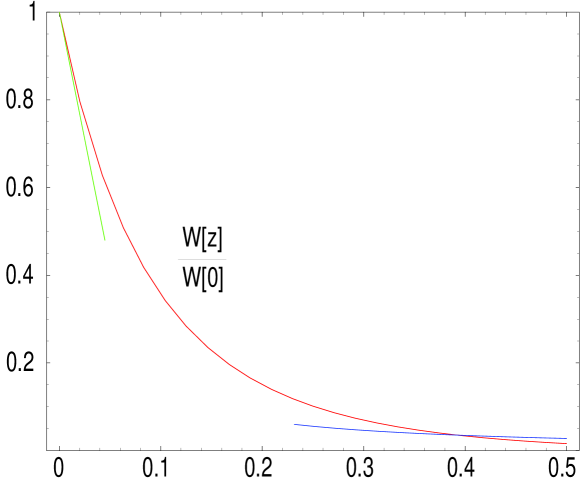
Figure 1: Plot of the hadronic function $W[z]$ in Eq. (3.1) versus $z=Q^{2}/\mu_{\mbox{\rm{\scriptsize had.}}}^{2}$ for $\mu_{\mbox{\rm{\scriptsize had.}}}=1.4\,\mbox{\rm GeV}$. The red curve is the normalized function $W[z]$ corresponding to the minimal hadronic ansatz discussed in the text, with a vector meson of mass $M_{V}=770\ \mbox{\rm MeV}$. The green line represents the low–energy chiral behaviour and the blue curve the prediction from the OPE.

Notice that, if we had had a perfect matching between the minimal hadronic ansatz and the OPE, we could have taken the limit $\hat{z}\rightarrow\infty$ in Eq. (4) and find again the same result as in Eq. (3.8) with the sum over hadronic states restricted to the lowest vector state. The fact that, as seen in Fig. 1, the matching is not perfect is not surprising; it is due to the restriction of the infinite sum in Eq. (3.1) to just the couplings of the lowest vector state. It is quite remarkable that, already at this approximation, the quality of the matching is so good. The advocated choice of a $\hat{z}$ which minimizes the value of $B_{K}$ at the separation between a low $Q^{2}$ region and a high $Q^{2}$ region implicitly assumes that the leading term of the OPE controls reasonably well the behaviour of the underlying Green’s function $W[z]$ down to $Q$ values in the region $0.8\,\mbox{\rm GeV}{\ \lower-1.2pt\vbox{\hbox{\hbox to0.0pt{$<$\hss}\lower 5.0pt\vbox{\hbox{$\sim$}}}}\ }Q{\ \lower-1.2pt\vbox{\hbox{\hbox to0.0pt{$<$\hss}\lower 5.0pt\vbox{\hbox{$\sim$}}}}\ }1\,\mbox{\rm GeV}$. 

In order to quantify the errors in Eq. (4.7) we proceed as follows: for every choice of $\mu_{\mbox{\rm{\scriptsize had.}}}$ one finds the corresponding value of $\hat{z}$ for which the hadronic ansatz and the OPE intersect. This value of $\hat{z}$ is then used in Eq. (4) to obtain $\hat{B}_{K}$. The error is estimated by allowing for a reasonable variation of the input parameters: $M_{V}=770\pm 30\ \mbox{\rm MeV}$ and $1$ GeV$\leq\mu_{\mbox{\rm{\scriptsize had.}}}\leq 3$ GeV. The corresponding values for $\hat{B}_{K}$ are given in Table 1. They correspond to the spread of values:

$$0.33\leq\hat{B}_{K}\leq 0.44\,.$$ (4.8)

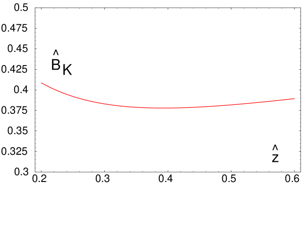
Figure 2: Plot of $\hat{B}_{K}$ in Eq. (4) versus $\hat{z}$, for $\mu_{\mbox{\rm{\scriptsize had.}}}\simeq 1.4\,\mbox{\rm GeV}$, $F_{0}=85.3\,\mbox{\rm MeV}$ and $M_{V}=770\,\mbox{\rm MeV}$. Notice the vertical scale in the figure.

Table 1: Summary of $\hat{B}_{K}$ results for different input values of $\mu_{\mbox{\rm{\scriptsize had.}}}$ and $M_{V}$

$M_{V}$	$\mu_{\mbox{\rm{\scriptsize had.}}}^{2}$
	$1\,\mbox{\rm GeV}^{2}$	$2\,\mbox{\rm GeV}^{2}$	$3\,\mbox{\rm GeV}^{2}$	$4\,\mbox{\rm GeV}^{2}$	$5\,\mbox{\rm GeV}^{2}$	$6\,\mbox{\rm GeV}^{2}$	$7\,\mbox{\rm GeV}^{2}$	$8\,\mbox{\rm GeV}^{2}$	$9\,\mbox{\rm GeV}^{2}$
$740\,\mbox{\rm MeV}$	0.387	0.413	0.421	0.426	0.429	0.431	0.433	0.434	0.435
$770\,\mbox{\rm MeV}$	0.388	0.413	0.422	0.426	0.429	0.432	0.433	0.435	0.436
$800\,\mbox{\rm MeV}$	0.329	0.342	0.346	0.347	0.348	0.349	0.350	0.350	0.350

One way to quantify the systematic error of the minimal hadronic ansatz approximation of this calculation would be to include in the analysis e.g. higher order terms in Eq. (3.3). Until we do that we suggest as a cautious rule-of-thumb estimate of this uncertainty to round off the spread in Eq. (4.8) to an overall $30\%$ of the central value, with the result

$$\hat{B}_{K}=0.38\pm 0.11\,.$$ (4.9)

Several remarks concerning this result are in order.

• Our result in Eq. (4.9) does not include the error due to next–to–next–to–leading terms in the $1/N_{c}$ expansion nor the error due to chiral corrections in the unfactorized contribution, but we consider it a rather robust prediction of $\hat{B}_{K}$ in the chiral limit and at the next-to-leading order in the $1/N_{c}$ expansion.

• Our calculation shows a crucial qualitative issue, which is the fact that the low–energy hadronic contribution below a mass scale $1\,\mbox{\rm GeV}{\ \lower-1.2pt\vbox{\hbox{\hbox to0.0pt{$<$\hss}\lower 5.0pt\vbox{\hbox{$\sim$}}}}\ }\mu_{\mbox{\rm{\scriptsize had.}}}{\ \lower-1.2pt\vbox{\hbox{\hbox to0.0pt{$<$\hss}\lower 5.0pt\vbox{\hbox{$\sim$}}}}\ }3\,\mbox{\rm GeV}$ brings down, rather dramatically, the value of $\hat{B}_{K}|_{\mbox{\rm{\scriptsize nll}}}$ in Eq. (4.2) evaluated at that scale. We can already conclude that any calculation which ”ignores” the details of the low–energy hadronic contribution will give an overestimate of $\hat{B}_{K}$.

• The result in Eq. (4.9) is compatible with the current algebra prediction [26] which, to lowest order in chiral perturbation theory, relates the $B_{K}$ factor to the $K^{+}\rightarrow\pi^{+}\pi^{0}$ decay rate. In fact, our calculation of the $B_{K}$ factor can be viewed as a successful prediction of the $K^{+}\rightarrow\pi^{+}\pi^{0}$ decay rate!

• As discussed in ref. [27] the bosonization of the four–quark operator $Q_{\Delta S=2}$ and the bosonization of the operator $Q_{2}-Q_{1}$ which generates $\Delta I=1/2$ transitions are related to each other in the combined chiral limit and next–to–leading order $1/N_{c}$ expansion. Lowering the value of $\hat{B}_{K}$ from the large–$N_{c}$ prediction in Eq. (1.9) to the result in Eq. (4.9) is correlated with an increase of the coupling constant in the lowest order effective chiral Lagrangian which generates $\Delta I=1/2$ transitions, and provides a first step towards a quantitative understanding of the dynamical origin of the $\Delta I=1/2$ rule.

• Finally, we wish to point out that the techniques applied here can be extended as well to include higher order terms in the chiral expansion. It remains to be seen if chiral corrections to the unfactorized term in Eq. (2.3) could be so large, (of order 100%?) as to increase our result in Eq. (4.9) to the values favoured by the lattice QCD determinations  as well as by recent phenomenological arguments [29].

Acknowledgments

We wish to thank Marc Knecht, Hans Bijnens and Ximo Prades for very helpful discussions on many topics related to the work reported here and to Maarten Golterman, Michel Perrottet and Toni Pich for discussions at various stages of this work. One of the authors (S.P.) is also grateful to C. Bernard and Y. Kuramashi for conversations and to the Physics Dept. of Washington University in Saint Louis for the hospitality extended to him while the earlier version of this work was being finished. This work has been supported in part by TMR, EC-Contract No. ERBFMRX-CT980169 (EURODA$\phi$NE). The work of S. Peris has also been partially supported by the research project CICYT-AEN99-0766.

References

[1]
G. Buchalla, A.J. Buras and M.E. Lautenbacher,
Rev. Mod. Phys. 68 (1996) 1125.
[2]
A.J. Buras, in Les Houches Lectures, Session LXVIII,
Probing the
Standard Model of Particle Interactions, eds. R. Gupta, A. Morel,
E. de Rafael and F. David, North–Holland 1999.
[3]
A. Pich and E. de Rafael, Nucl. Phys. B358 (1991) 311.
[4]
E. de Rafael, “Chiral Lagrangians and Kaon CP–Violation”, in
CP Violation and the Limits of the Standard Model, Proc.
TASI’94, ed. J.F. Donoghue (World Scientific, Singapore, 1995)