Abstract

We present the results of a quenched lattice calculation of the operator matrix elements relevant for predicting the $B_{s}$ width difference. Our main result is $\left(\Delta\Gamma_{B_{s}}/\Gamma_{B_{s}}\right)=(4.7\pm 1.5\pm 1.6)\times 10^{-2}$, obtained from the ratio of matrix elements ${\cal R}(m_{b})=\langle\bar{B}_{s}^{0}|Q_{S}|B_{s}^{0}\rangle/\langle\bar{B}_{s}^{0}|Q_{L}|B_{s}^{0}\rangle=-0.93(3)^{+0.00}_{-0.01}$. ${\cal R}(m_{b})$ was evaluated from the two relevant $B$-parameters $B_{S}^{\overline{\rm MS}}(m_{b})=0.86(2)^{+0.02}_{-0.03}$ and $B_{B_{s}}^{\overline{\rm MS}}(m_{b})=0.91(3)^{+0.00}_{-0.06}$, which we computed in our simulation.

 

PACS: 13.75Lb, 11.15.Ha, 12.38.Gc.

1 Introduction

In the Standard Model, the width difference $\left(\Delta\Gamma_{B_{s}}/\Gamma_{B_{s}}\right)$ of $B_{s}$ mesons is expected to be rather large and within reach for being measured in the near future. Recent experimental studies [1, 2] already provide an interesting bound on this quantity. In particular, in ref. [2] the limit $\left(\Delta\Gamma_{B_{s}}/\Gamma_{B_{s}}\right)<0.31$ $(95\%C.L.)$ is quoted .

Theoretically, the prediction of $\left(\Delta\Gamma/\Gamma\right)_{B_{s}}$ relies on the use of the operator product expansion (OPE), where the large scale is provided by the heavy quark mass [3]. All recent developments, including the calculation of the next-to-leading order (NLO) perturbative QCD corrections, have been discussed in great detail in refs. [4]–[6]. The theoretical estimates are in the range $\left(\Delta\Gamma_{B_{s}}/\Gamma_{B_{s}}\right)=(5\div 15)\%$ and crucially depend on the size of relevant hadronic matrix elements which must be computed non-perturbatively.

In this paper we present a new lattice calculation of the main contribution to $(\Delta\Gamma_{B_{s}}/\Gamma_{B_{s}})$. On the basis of our results, and using the expressions given below, we predict

$$\frac{\Delta\Gamma_{B_{s}}}{\Gamma_{B_{s}}}=(4.7\pm 1.5\pm 1.6)\times 10^{-2}\,,$$ (1)

where the last error is obtained by assuming an uncertainty of $30\%$ on the $1/m_{b}$ corrections.

We now present the relevant formulae which have been used to get the prediction in eq. (1). Up and including $1/m_{b}$ corrections, the theoretical expression for $\left(\Delta\Gamma_{B_{s}}/\Gamma_{B_{s}}\right)$ reads [4]

$${\Delta\Gamma_{B_{s}}\over\Gamma_{B_{s}}}={G_{F}^{2}m_{b}^{2}\over 12\pi m_{B_{s}}}\left|{V_{cb}V_{cs}}\right|^{2}\tau_{B_{s}}\biggl{(}G(z)\langle Q_{L}(m_{b})\rangle-G_{S}(z)\langle Q_{S}(m_{b})\rangle+\delta_{1/m}\sqrt{1-4z}\biggr{)}\;,$$ (2)

where $z=m_{c}^{2}/m_{b}^{2}$ and $G(z)$ and $G_{S}(z)$ are functions which have been computed in perturbation theory at the next-to-leading order (NLO) [6]. $\langle Q_{L,S}\rangle=\langle\bar{B}_{s}^{0}|Q_{L,S}|B_{s}^{0}\rangle$ are the hadronic matrix elements of the renormalized operators relevant at the lowest order in the heavy quark expansion

$$Q_{L} = \bar{b}^{i}\gamma^{\mu}(1-\gamma_{5})s^{i}\ \bar{b}^{j}\gamma_{\mu}(1-\gamma_{5})s^{j}$$ (3)

$$Q_{S} = \bar{b}^{i}(1-\gamma_{5})s^{i}\ \bar{b}^{j}(1-\gamma_{5})s^{j}\,,$$ (5)

where $i$ and $j$ are colour indices. The last term in eq. (2), $\delta_{1/m}\sqrt{1-4z}$, represents the contribution of $1/m_{b}$ corrections.

In order to reduce the uncertainties of the theoretical predictions, it is convenient to consider the ratio of the width and mass differences of the $B_{s}^{0}$–$\bar{B}_{s}^{0}$ system

$${\Delta\Gamma_{B_{s}}\over\Delta m_{B_{s}}}={4\pi\over 3}{m_{b}^{2}\over m_{W}^{2}}\left|{V_{cb}V_{cs}\over V_{ts}V_{tb}}\right|^{2}{1\over\eta_{B}(m_{b})S_{0}(x_{t})}\left(G(z)-G_{S}(z){\langle Q_{S}\rangle\over\langle Q_{L}\rangle}+\tilde{\delta}_{1/m}\right)\;,$$ (6)

where $\eta_{B}(m_{b})$ has been computed in perturbation theory to NLO [7] and $S_{0}(x_{t})$ is the usual Inami-Lim function [8]. Note that, to make contact with ref. [6], in the above formulae we used the $\overline{\rm MS}$ coefficient $\eta_{B}(m_{b})$ instead of the standard $\eta_{B}$ of ref. [7]. Consequently, the operators $Q_{S}$ and $Q_{L}$ are renormalized in the $\overline{\rm MS}$ (NDR) scheme. We see from eq. (6), that $(\Delta\Gamma_{B_{s}}/\Delta m_{B_{s}})$ only depends on the ratio of matrix elements,

$${\cal R}(m_{b})={\langle Q_{S}\rangle\over\langle Q_{L}\rangle}={\langle\bar{B}_{s}^{0}|Q_{S}(m_{b})|B_{s}^{0}\rangle\over\langle\bar{B}_{s}^{0}|Q_{L}(m_{b})|B_{s}^{0}\rangle}\ ,$$ (7)

which may, in principle, be directly determined on the lattice. The use of ${\cal R}$ is particularly convenient because dimensionless quantities are not affected by the uncertainty due to the calibration of the lattice spacing. One may also argue that many systematic errors, induced by discretization and quenching, cancel in the ratio of two similar amplitudes.

Finally, eq. (6) allows to express $(\Delta\Gamma_{B_{s}}/\Gamma_{B_{s}})$ in terms of i) perturbative quantities, encoded in the overall factor and in the functions $G(z)$ and $G_{S}(z)$, ii) a lattice measured quantity, ${\cal R}$ and iii) $\Delta m_{B_{s}}$ which will be hopefully precisely measured in the near future:

$${\Delta\Gamma_{B_{s}}\over\Gamma_{B_{s}}}\ =\ \left(\tau_{B_{s}}\Delta m_{B_{s}}\right)^{\rm(exp.)}\ {K}\times\left(G(z)-G_{S}(z){\cal R}(m_{b})+\tilde{\delta}_{1/m}\right)\ ,$$ (8)

where

$$K={4\pi\over 3}{m_{b}^{2}\over m_{W}^{2}}\left|{V_{cb}V_{cs}\over V_{ts}V_{tb}}\right|^{2}{1\over\eta_{B}(m_{b})S_{0}(x_{t})}\ ,$$ (9)

Waiting the measurement of $\Delta m_{B_{s}}$, for which only a lower bound presently exists [9], one can use a modified version of eq. (8), namely

$${\Delta\Gamma_{B_{s}}\over\Gamma_{B_{s}}}\ =\ \left(\tau_{B_{s}}\Delta m_{B_{d}}\frac{m_{B_{s}}}{m_{B_{d}}}\right)^{\rm(exp.)}\ \left|V_{ts}\over V_{td}\right|^{2}{K}\cdot\biggl{(}G(z)-G_{S}(z){\cal R}(m_{b})+\tilde{\delta}_{1/m}\biggr{)}\ \xi^{2}\ ,$$ (10)

where

$$\xi=\frac{f_{B_{s}}\sqrt{\hat{B}_{B_{s}}}}{f_{B_{d}}\sqrt{\hat{B}_{B_{d}}}}\ .$$ (11)

In this way, besides the quantities discussed above, we only use the experimental $B_{d}$-meson mass difference, which is known with a tiny error [2]

$$\left(\Delta m_{B_{d}}\right)^{\rm(exp.)}=0.484(15)\,ps^{-1}\ ,$$ (12)

and another ratio of hadronic matrix elements, namely $\xi$, which is rather accurately determined in lattice simulations [10, 11].

For the following discussion, it is useful to write eq. (10) as (note the ${\cal R}(m_{b})$ is negative)

$${\Delta\Gamma_{B_{s}}\over\Gamma_{B_{s}}}\ =\left[(0.5\pm 0.1)-(13.8\pm 2.8){\cal R}(m_{b})+(15.7\pm 2.8)\tilde{\delta}_{1/m}\right]\times 10^{-2}\,,$$ (13)

where the three contributions correspond to $G(z)$, $-G_{S}(z){\cal R}(m_{b})$ and $\tilde{\delta}_{1/m}$ in (10), respectively.

The advantage of using eqs. (6), (8) and (10) consists also in the fact that, in order to predict $\left(\Delta\Gamma_{B_{s}}/\Gamma_{B_{s}}\right)$, we do not need $f_{B_{s}}$, which enters eq. (2) when we express the matrix elements in terms of $B$-parameters. There is still a considerable uncertainty, indeed, on $f_{B_{s}}$, which has been evaluated both in the quenched ($f_{B_{s}}=195\pm 20$ MeV) and unquenched ($f_{B_{s}}=245\pm 30$ MeV) case, with a sizeable shift between the two central values [10]. Since the “unquenched” results are still in their infancy, however, we think that the large quenching effect should not be taken too seriously yet.

In the numerical evaluation of the width difference, we have used the values and errors of the parameters given in Tab. 1. For the perturbative quantities $G(z)$ and $G_{S}(z)$, the main uncertainty comes from dependence on the renormalization scale, which was varied between $m_{b}/2$ and $2m_{b}$ in ref. [6] (with $m_{b}=4.8$ GeV). For this reason, we found it useless to recompute these coefficients with $m_{b}=4.6$ GeV (which is very close to the mass used in [6]). Instead, we took as central value the average $G_{S}(z)=(G_{S}^{\mu_{1}=m_{b}/2}(z)+G_{S}^{\mu_{1}=2\ m_{b}}(z))/2$ (see Tab. 1 of that paper), and as error $(G_{S}^{\mu_{1}=m_{b}/2}(z)-G_{S}^{\mu_{1}=2\ m_{b}}(z))/2$. The same was made in the case of $G(z)$.

For the hadronic quantities, we have used the following values

$${\cal R}(m_{b})=-0.93(3)^{+0.00}_{-0.01}\ ,\quad\quad\xi=1.16(7)\ ,$$ (14)

${\cal R}(m_{b})$ is the main results of this lattice study, while the result for $\xi$ has already been reported in our previous paper [11]. Following ref. [4], for the $1/m_{b}$ corrections we get

$$\delta_{1/m}=-2.0\,\mbox{GeV}^{4}\;,$$ (15)

using $f_{B_{s}}=204$ MeV from ref. [11]. This value of $\delta_{1/m}$ corresponds to $\tilde{\delta}_{1/m}=-0.55$ (obtained with $B_{B_{s}}^{\overline{\rm MS}}(m_{b})=0.91$) . Since in the estimate of $\tilde{\delta}_{1/m}$, the operator matrix elements were computed in the vacuum saturation approximation (VSA), and the radiative corrections were not included, we allow it to vary by $30\%$, i.e. $\tilde{\delta}_{1/m}=-0.55\pm 0.17$. In the numerical evaluation of the factor $K$, we have used the pôle mass $m_{b}=4.6$ GeV derived from the $\overline{\rm MS}$ mass in Tab. 1 at the NLO. Using these numbers, from eq. (10) we obtain the result in eq. (1), where the last error comes from the uncertainty on $\tilde{\delta}_{1/m}$.

We have an important remark to make. Eq. (13) shows explicitly the cancellation occurring between the main contribution, proportional to ${\cal R}(m_{b})$, and the $1/m_{b}$ corrections, proportional to $\tilde{\delta}_{1/m}$. Without the latter, we would have found a much larger value, $\left(\Delta\Gamma_{B_{s}}/\Gamma_{B_{s}}\right)\simeq 14\times 10^{-2}$. $\left(\Delta\Gamma_{B_{s}}/\Gamma_{B_{s}}\right)$ would remain in the $10\%$ range even with a sizeable, but smaller, value for the $1/m_{b}$ term, $\tilde{\delta}_{1/m}=-0.30$ for example. This demonstrates that, in spite of the progress made in the evaluation of the relevant matrix elements ($\langle Q_{S}\rangle$ and $\langle Q_{L}\rangle$), a precise determination of the width difference requires a good control of the subleading terms in the $1/m_{b}$ expansion, which is missing to date.

lj Parameter	Value and error
$m_{W}$	80.41 GeV
$m_{B_{d}}$	5.279 GeV
$m_{B_{s}}$	5.369 GeV
$\tau_{B_{s}}$	$1.460\pm 0.056\,ps$
$|V_{cb}|$	$0.0395\pm 0.0017$
$|V_{ts}|$	$0.0386\pm 0.0013$
$|V_{cs}|$	$0.9759\pm 0.0005$
$|V_{td}|$	$0.0080\pm 0.0005$
$\alpha_{s}(M_{Z})$	$0.118\pm 0.003$
$\Delta m_{B_{d}}$	$0.484\pm 0.015\,ps^{-1}$
$m_{t}$	$165\pm 5$ GeV
$m_{b}$	$4.23\pm 0.07$ GeV
$m_{c}/m_{b}$	$0.29\pm 0.02$
$m_{s}$	$110\pm 20$ MeV
$\eta_{B}(m_{b})$	$0.85\pm 0.02$
$G(z)$	$0.030\pm 0.007$
$G_{S}(z)$	$0.88\pm 0.14$

Table 1: Average and errors of the main parameters. When the error is negligible it has been omitted. The heavy-quark masses ($m_{t}$, $m_{b}$ and $m_{c}$) are the $\overline{\rm MS}$ masses renormalized at their own values, e.g. $m_{t}=m_{t}^{\scriptsize{\overline{\rm MS}}}(m_{t}^{\scriptsize{\overline{\rm MS}}})$. $m_{s}=m_{s}^{\scriptsize{\overline{\rm MS}}}(\mu=2\,\mbox{GeV})$ is the strange quark mass renormalized in $\overline{\rm MS}$ at the scale $\mu=2$ GeV. Its central value and error are not important in the numerical evaluation of $\Delta\Gamma_{B_{s}}$.

One can also use eq. (8), and combine it with [9]

$$\left(\Delta m_{B_{s}}\right)^{\rm(exp.)}>14.6\ ps^{-1}\ ,$$ (16)

to obtain a lower bound on $(\Delta\Gamma_{B_{s}}/\Gamma_{B_{s}})$. Given the large uncertainties, this bound is at present rather weak. At the 1-$\sigma$ level we get

$$\frac{\Delta\Gamma_{B_{s}}}{\Gamma_{B_{s}}}>2.5\times 10^{-2}\,\,\,\,(68\%\mbox{C.L.})\ .$$ (17)

Following ref. [2], from eq. (8) and the limit $\left(\Delta\Gamma_{B_{s}}/\Gamma_{B_{s}}\right)<0.31$, we could also obtain an upper limit on $\Delta m_{B_{s}}$. In our case this is not very interesting, however, since we find a very large upper bound of ${\cal O}(200)\ ps^{-1}$.

Our prediction in eq. (1) is in good agreement with ref. [6]. It is instead about a factor of two smaller than the result of ref. [17]. A detailed comparison of the two lattice calculations can be found in sec. 4.

We stress that the theoretical formulae should be evaluated with hadronic parameters computed in a coherent way, within the same lattice calculation, and not from different calculations (the “Arlequin” procedure according to ref. [12]), since their values and errors are correlated. All our lattice results were obtained using a non-perturbatively improved action [13], and with operators renormalized on the lattice with the non-perturbative method of ref. [14], as implemented in [15, 16]. Our new result is ${\cal R}(m_{b})$. For completeness, we also present some relevant $B$-parameters which enter the calculation of the mixing and width difference

$$B_{S}^{\overline{\rm MS}}(m_{b})=0.86(2)^{+0.02}_{-0.03}\;,\quad B_{B_{s}}^{\overline{\rm MS}}(m_{b})=0.91(3)^{+0.00}_{-0.06}\;.$$ (18)

The remainder of this paper is as follows: in sec. 2 we discuss the renormalization of the relevant operators and the calculation of their matrix elements; the extrapolation to the physical points and the evaluation of the statistical and systematic errors are presented in sec. 3; sec. 4 contains a comparison of our results with other calculations of the same quantities as well as our conclusions.

2 Calculation of the Matrix Elements

In this section, we discuss the construction of the renormalized operators which enter the prediction of $\Delta\Gamma_{B_{s}}$ and describe the extraction of their matrix elements in our simulation.

Besides the operators in eq. (3), we also need

$${\tilde{Q}}_{S} = \ \bar{b}^{i}(1-\gamma_{5})s^{j}\,\bar{b}^{j}(1-\gamma_{5})s^{i}\,,$$

$${Q}_{P} = \ \bar{b}^{i}(1-\gamma_{5})s^{i}\,\bar{b}^{j}(1+\gamma_{5})s^{j}\,,$$ (19)

$${\tilde{Q}}_{P} = \ \bar{b}^{i}(1-\gamma_{5})s^{j}\,\bar{b}^{j}(1+\gamma_{5})s^{i}\,.$$

The five operators in eqs. (3) and (2) form a complete basis necessary for the lattice subtractions which will be discussed later on. In ref. [18], a new method, that allows the calculation of $\Delta F=2$ amplitudes without subtractions, has been proposed and feasibility studies are underway. If successful, it will be obviously applied also to the calculation of $\Delta\Gamma_{B_{s}}$.

The matrix elements which contribute to $\Delta\Gamma_{B_{s}}$ are traditionally computed in terms of their value in the vacuum saturation approximation (VSA), by introducing the so called $B$-parameters. The latter encode the mismatch between full QCD and VSA values. There is a certain freedom in defining the $B$-parameters (see for example the discussion in ref. [19]). For $Q_{S}$ and $\tilde{Q}_{S}$, two equivalent definitions will be used in the following

$$\langle\bar{B}^{0}_{q}|{Q_{L}}(\mu)|B^{0}_{q}\rangle = \frac{8}{3}\ m_{B_{s}}^{2}f_{B_{s}}^{2}\ B_{B_{s}}(\mu)\,,$$ (20)

j (21)

$$\langle\bar{B}^{0}_{q}|{Q}_{S}(\mu)|B^{0}_{q}\rangle = -\frac{5}{3}\ \left({m_{B_{s}}\over m_{b}(\mu)+m_{s}(\mu)}\right)^{2}m_{B_{s}}^{2}f_{B_{s}}^{2}\ B_{S}(\mu)\equiv-\frac{5}{3}m_{B_{s}}^{2}f_{B_{s}}^{2}B_{S}^{\prime}(\mu)\,,$$ (22)

j (23)

$$\langle\bar{B}^{0}_{q}|{\tilde{Q}}_{S}(\mu)|B_{q}\rangle = \frac{1}{3}\ \left({m_{B_{s}}\over m_{b}(\mu)+m_{s}(\mu)}\right)^{2}m_{B_{s}}^{2}f_{B_{s}}^{2}\ \tilde{B}_{S}(\mu)\equiv\frac{1}{3}m_{B_{s}}^{2}f_{B_{s}}^{2}\tilde{B}_{S}^{\prime}(\mu)\,.$$ (24)

The first definition is the traditional one that requires, for the physical matrix elements, the knowledge of the quark masses; the second one may present some advantage, because the matrix elements are derived using physical quantities only ($m_{B_{s}}$ and $f_{B_{s}}$). The label $(\mu)$ denotes that operators and quark masses are renormalized, in a given renormalization scheme ($\overline{\rm MS}$ in our case) at the scale $\mu$. Since the matrix element of the first operator, essential for $\bar{B}_{s}^{0}$–$B^{0}_{s}$ mixing, was studied in detail in our previous paper [11], here we only consider the two other relevant operators, namely $Q_{S}$ and $\tilde{Q}_{S}$.

2.1 Matrix elements from correlation functions

Before presenting our results, let us recall the main steps necessary to extract the matrix elements in numerical simulations. As usual, one starts from the (Euclidean) three-point correlation functions:

$${\cal C}^{(3)}_{i}(t_{P_{1}},t_{P_{2}})=\displaystyle{\sum_{\vec{x},\vec{y}}}\ \langle 0|P_{5}(\vec{x},-t_{P_{2}}){Q}_{i}(0)P_{5}(\vec{y},t_{P_{1}})|0\rangle\ ,$$ (25)

where $Q_{i}$ denotes any of the operators enumerated in eqs. (3) and (2). When the $Q_{i}$ and the sources $P_{5}$ (which we choose to be $P_{5}=i\bar{s}\gamma_{5}b$) are sufficiently separated in time, the lightest pseudoscalar-meson contribution dominates the correlation functions and the matrix elements can be extracted

$${\cal C}^{(3)}_{i}(t_{P_{1}},t_{P_{2}})\stackrel{{\scriptstyle t_{P_{1}},t_{P_{2}}\gg 0}}{{\longrightarrow}}\,{\sqrt{{\cal{Z}}_{P}}\over 2M_{P}}e^{-M_{P}t_{P_{1}}}\ \langle\bar{P}|{Q}_{i}(a)|P\rangle\ {\sqrt{{\cal{Z}}_{P}}\over 2M_{P}}e^{-M_{P}t_{P_{2}}},$$ (26)

where $\sqrt{{\cal{Z}}_{P}}=|\langle 0|P_{5}|P\rangle|$. We take both mesons at rest and label the bare operators on the lattice as ${Q}_{i}(a)$, to distinguish them from their continuum counterparts. The matching to the continuum renormalized operators is what we discuss next.

2.2 Operator Matching and Renormalization

In this subsection, we describe the procedure used to get the renormalized operator ${Q}_{S}(\mu)$, relevant in the calculation of $\Delta\Gamma_{B_{s}}$, from the lattice bare operators. This is achieved through a two steps procedure:

• We define the subtracted operators ${Q^{\prime}}_{S}$ and $\tilde{Q}^{\prime}_{S}$, obeying to the continuum Ward identities (up to corrections of ${\cal O}(a)$), as

  $${Q^{\prime}}_{S}={Q}_{S}(a)+\sum_{i=L,P,\tilde{P}}\Delta_{i}(g_{0}^{2}){Q}_{i}(a)\ ,$$ (27)

  (28)

  $${\tilde{Q}^{\prime}}_{S}={\tilde{Q}}_{S}(a)+\sum_{i=L,P,\tilde{P}}\widetilde{\Delta}_{i}(g_{0}^{2}){Q}_{i}(a)\ .$$ (29)

  The constants $\Delta_{i}(g_{0}^{2})$, which we calculate using the non-perturbative method discussed in refs. [15, 16], are listed in Tab. 2. Note that the mixing (27) is a lattice artifact (as a consequence of the explicit chiral symmetry breaking in the Wilson action) and the subtraction ensures that the resulting operators, ${Q^{\prime}}_{S}$ and $\tilde{Q}^{\prime}_{S}$, have the same chiral properties as in the continuum.

  In principle, the mixing coefficients $\Delta_{i}(g_{0}^{2})$ are functions of the bare coupling constant $g_{0}^{2}$ only. Therefore, at fixed lattice spacing, they should be independent of the scale at which the operators are renormalized. In practice, due to some systematic effects, they may depend on the renormalization scale (which corresponds to the virtuality of the external quark legs). This induces an uncertainty in the determination of the physical matrix elements which will be accounted for in the estimate of the systematic error.

• CPS symmetry allows the mixing of ${Q}_{S}$ and ${\tilde{Q}}_{S}$ under renormalization. This is why we must consider both of them, although our main target is the matrix element of the renormalized ${Q}_{S}(\mu)$. In the second step, the operators are renormalized as:

  $$\left(\begin{array}[]{c}{Q}_{S}(\mu)\\ {\tilde{Q}}_{S}(\mu)\\ \end{array}\right)\ =\ \left(\begin{array}[]{cc}Z_{22}(\mu)&Z_{23}(\mu)\\ Z_{32}(\mu)&Z_{33}(\mu)\\ \end{array}\right)\ \left(\begin{array}[]{c}{Q^{\prime}}_{S}\\ {\tilde{Q}^{\prime}}_{S}\\ \end{array}\right)\;,$$ (36)

  where the structure of mixing ($Z_{23}\neq Z_{32}\neq 0$) is the same as in the continuum. We compute the renormalization matrix non-perturbatively by using the method of ref. [16], in the Landau RI-MOM renormalization scheme. The results for three values of the renormalization scale, $\mu=\{$ $1.9$ GeV, $2.7$ GeV, $3.8$ GeV $\}$, are given in Tab. 2.

lj Scale $\mu$	$\Delta_{L}$	$\Delta_{P}$	$\Delta_{\tilde{P}}$	$\widetilde{\Delta}_{L}$	$\widetilde{\Delta}_{P}$	$\widetilde{\Delta}_{\tilde{P}}$
lj 1.9 GeV	0.005(1)	0.219(8)	-0.016(8)	-0.002(0)	-0.094(3)	0.007(3)
lj 2.7 GeV	0.003(0)	0.175(5)	-0.014(2)	-0.001(0)	-0.075(2)	0.005(1)
lj 3.8 GeV	0.002(1)	0.189(3)	-0.012(2)	-0.001(0)	-0.081(1)	0.003(1)

lj Scale $\mu$	$Z_{22}(\mu)$	$Z_{23}(\mu)$	$Z_{32}(\mu)$	$Z_{33}(\mu)$
lj 1.9 GeV	0.237(13)	-0.122(16)	0.313(1)	1.018(5)
lj 2.7 GeV	0.282(12)	-0.128(16)	0.229(0)	0.883(3)
lj 3.8 GeV	0.332(12)	-0.184(16)	0.203(1)	0.902(0)

Table 2: Numerical results for the $\Delta(g_{0}^{2})$s and the matrix $Z(g_{0}^{2},\mu)$. They have been evaluated non-perturbatively in the Landau RI-MOM scheme, at $\beta=6/g_{0}^{2}=6.2$, at the three different scales $\mu$ given in the table.

2.3 Extraction of the B-parameters

Equipped with suitably renormalized operators in the RI-MOM scheme, we proceed by removing the external meson propagators and sources from the correlation functions. This can be done in two ways. From the ratios

$${{\cal C}^{(3)}_{S}(t_{P_{1}},t_{P_{2}};\mu)\over\ -{5\over 3}Z_{A}^{2}{\cal C}_{AP}^{(2)}(t_{P_{2}})\ {\cal C}_{AP}^{(2)}(t_{P_{1}})}\ \to\ {\langle\bar{P}|{Q}_{S}(\mu)|P\rangle\over-{5\over 3}|\langle 0|\hat{A}_{0}|P\rangle|^{2}}\ \equiv B_{S}^{\prime}(\mu)\ ,$$ (37)

(38)

(39)

$${{\cal C}^{(3)}_{\tilde{S}}(t_{P_{1}},t_{P_{2}};\mu)\over\ {1\over 3}Z_{A}^{2}{\cal C}_{AP}^{(2)}(t_{P_{2}})\ {\cal C}_{AP}^{(2)}(t_{P_{1}})}\ \to\ {\langle\bar{P}|{\tilde{Q}}_{S}(\mu)|P\rangle\over{1\over 3}|\langle 0|\hat{A}_{0}|P\rangle|^{2}}\ \equiv\tilde{B}_{S}^{\prime}(\mu)$$ (40)

we extract the $B^{\prime}$-parameters (Method-I). The quality of the resulting plateaus is illustrated in Fig. 1. Since the lattice renormalization constant of the axial current ($\hat{A}_{0}=Z_{A}\bar{s}\gamma_{0}\gamma_{5}b$) is $\mu$-independent, the anomalous dimension of the parameter ${B}_{S}^{\prime}(\mu)$ is exactly the same as for $\langle{Q}_{S}(\mu)\rangle$.

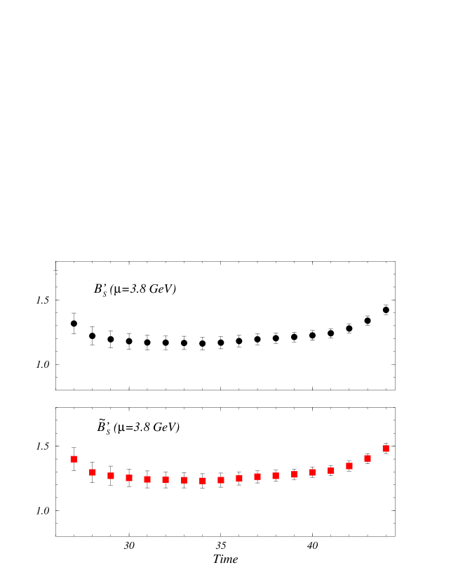
Figure 1: The ratios defined in eq. (37) are shown as a function of ${\rm Time}=-t_{P_{2}}$ at fixed $t_{P_{1}}=16$. All quantities are in lattice units. The figure refers to $\kappa_{q}=0.1349$ and $\kappa_{Q}=0.1220$.

On the other hand, if we combine the correlation functions in the ratios:

$${{\cal C}^{(3)}_{S}(t_{P_{1}},t_{P_{2}};\mu)\over\ -{5\over 3}Z^{2}_{P}(\mu){\cal C}_{PP}^{(2)}(t_{P_{2}};\mu)\ {\cal C}_{PP}^{(2)}(t_{P_{1}};\mu)}\ \to\ {\langle\bar{P}|{Q}_{S}(\mu)|P\rangle\over-{5\over 3}|\langle 0|\hat{P}_{5}(\mu)|P\rangle|^{2}}\ \equiv B_{S}(\mu)\ ,$$ (41)

(42)

(43)

$${{\cal C}^{(3)}_{\tilde{S}}(t_{P_{1}},t_{P_{2}};\mu)\over\ {1\over 3}Z^{2}_{P}(\mu){\cal C}_{PP}^{(2)}(t_{P_{2}};\mu)\ {\cal C}_{PP}^{(2)}(t_{P_{1}};\mu)}\ \to\ {\langle\bar{P}|{\tilde{Q}}_{S}(\mu)|P\rangle\over{1\over 3}|\langle 0|\hat{P}_{5}(\mu)|P\rangle|^{2}}\ \equiv\tilde{B}_{S}(\mu)\ .$$ (44)

we get the standard $B$-parameters (Method-II). The plateaus are shown in Fig. 2.

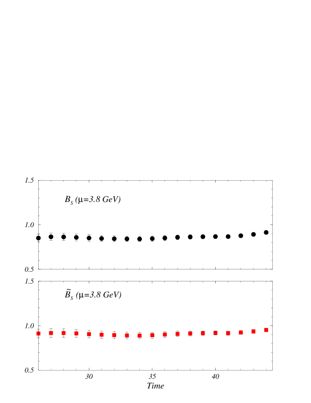
Figure 2: As in Fig. 1. for the standard $B_{S}$ and $\tilde{B}_{S}$, as specified in eq. (41).

In the above ratios, we have used the renormalized pseudoscalar density, $\hat{P}_{5}(\mu)=iZ_{P}(\mu)\bar{s}\gamma_{5}b$. The value of $Z_{P}(\mu)$ is also obtained non-perturbatively in the way described in ref. [14]. Numerically (and in the chiral limit), we have $Z_{P}(\mu)=\{0.43(2),0.45(2),0.50(2)\}$ in increasing order of $\mu$.

The second method has the advantage that the (rather large) $\mu$-dependence of the operator $\langle{Q}_{S}(\mu)\rangle$ is almost cancelled by the anomalous dimension of the squared renormalized pseudoscalar density. On the other hand, the first method seems more convenient because physical amplitudes can be obtained without introducing the quark masses, which are a further source of theoretical uncertainty. We found, however, that $B^{\prime}_{S}$ has a very strong dependence on the heavy quark mass, which prevents a reliable extrapolation to $m_{B_{s}}$. Before discussing the subtleties related to the extrapolation, we present our results for the heavy-light meson masses directly accessible in our simulation.

2.4 $B$-parameters in the Landau RI-MOM scheme

In this subsection we present the results for both sets of $B$-parameters. As in our previous paper [11], our study is based on a sample of $200$ independent quenched gauge field configurations, generated at the coupling constant $\beta=6.2$, on the volume $24^{3}\times 48$. We use three values of the hopping parameter corresponding to the light quark mass ($\kappa_{q}=$ $0.1344$, $0.1349$, $0.1352$), and three values corresponding to the heavy quarks ($\kappa_{Q}=$ $0.125$, $0.122$, $0.119$). The first source is kept fixed at $t_{P_{1}}=16$, while the second one moves along the temporal axis. The 4-fermion operator under study is inserted at the origin ($t=0$). After examining the plateaus of the different ratios in eqs. (37) and (41), for every combination of the hopping parameters, we choose to fit in the time intervals, $t_{B_{S}}\ \in\ [31,34]$ and $t_{\tilde{B}_{S}}\ \in\ [32,35]$. We present results for each value of $\kappa_{Q}$, with the light quark interpolated to the $s$-quark or extrapolated to the $d$-quark. For a generic $B$-parameter, this is obtained by fitting our data to the following expression:

$${B}(m_{Q},m_{q})=\alpha_{0}^{Q}+\alpha_{1}^{Q}M^{2}_{P}(m_{q},m_{q})\,.$$ (45)

This is illustrated in Fig. 3, while a detailed list of results is presented in Tabs. 3 and 4.

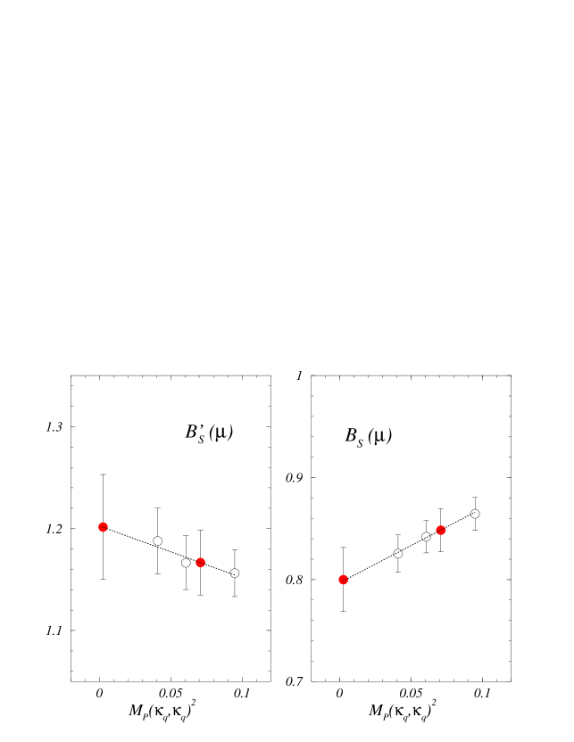
Figure 3: Fit in the light quark mass of ${B}_{S}(\mu)$ and $B_{S}^{\prime}(\mu)$ (at $\mu=3.8$ GeV) according to eq. (45). Empty symbols denote data obtained from our simulation, whereas filled symbols denote quantities obtained after interpolation (extrapolation) to the strange (up-down) light quark mass. The heavy-quark mass corresponds to $\kappa_{Q_{2}}=0.1220$.

lj $\mu$	$1.9$ GeV		$2.7$ GeV		$3.8$ GeV
lj Light quark	$q=s$	$q=d$	$q=s$	$q=d$	$q=s$	$q=d$
lj $B_{S}^{\prime}(\mu;\kappa_{Q}=0.1250)$	0.93(3)	0.98(5)	1.15(4)	1.21(6)	1.32(4)	1.38(7)
lj $\tilde{B}_{S}^{\prime}(\mu;\kappa_{Q}=0.1250)$	0.99(4)	1.06(6)	1.21(4)	1.29(6)	1.41(5)	1.49(7)
lj $B_{S}^{\prime}(\mu;\kappa_{Q}=0.1220)$	0.83(3)	0.85(4)	1.02(3)	1.05(5)	1.17(4)	1.20(5)
lj $\tilde{B}_{S}^{\prime}(\mu;\kappa_{Q}=0.1220)$	0.87(3)	0.91(5)	1.06(3)	1.10(5)	1.23(4)	1.28(6)
lj $B_{S}^{\prime}(\mu;\kappa_{Q}=0.1190)$	0.75(2)	0.77(3)	0.91(2)	0.94(4)	1.05(3)	1.08(4)
lj $\tilde{B}_{S}^{\prime}(\mu;\kappa_{Q}=0.1190)$	0.77(3)	0.82(4)	0.94(3)	0.99(4)	1.10(3)	1.15(5)

Table 3: Results for $B_{S}^{\prime}(\mu)$ and $\tilde{B}_{S}^{\prime}(\mu)$ in the Landau RI-MOM scheme. The light quark mass is extrapolated/interpolated to $d/s$ quarks.

lj $\mu$	$1.9$ GeV		$2.7$ GeV		$3.8$ GeV
lj Light quark	$q=s$	$q=d$	$q=s$	$q=d$	$q=s$	$q=d$
lj $B_{S}(\mu;\kappa_{Q}=0.1250)$	0.87(3)	0.84(4)	0.85(2)	0.82(3)	0.87(2)	0.79(3)
lj $\tilde{B}_{S}(\mu;\kappa_{Q}=0.1250)$	0.92(3)	0.91(4)	0.90(3)	0.88(4)	0.88(3)	0.86(4)
lj $B_{S}(\mu;\kappa_{Q}=0.1220)$	0.90(3)	0.85(4)	0.88(2)	0.83(3)	0.85(2)	0.80(3)
lj $\tilde{B}_{S}(\mu;\kappa_{Q}=0.1220)$	0.94(3)	0.91(4)	0.92(2)	0.88(4)	0.90(2)	0.86(4)
lj $B_{S}(\mu;\kappa_{Q}=0.1190)$	0.92(2)	0.91(3)	0.90(2)	0.89(3)	0.87(2)	0.86(3)
lj $\tilde{B}_{S}(\mu;\kappa_{Q}=0.1190)$	0.95(3)	0.96(4)	0.93(2)	0.94(3)	0.91(2)	0.91(3)

Table 4: As in Tab. 3, but for $B_{S}(\mu)$ and $\tilde{B}_{S}(\mu)$.

At this point we have obtained the matrix elements parameterized in two ways ( $B_{S}^{\prime}(\mu)$–$\tilde{B}_{S}^{\prime}(\mu)$ and $B_{S}(\mu)$–$\tilde{B}_{S}(\mu)$, respectively) in the RI-MOM scheme, at three values of the heavy quark masses (around the charm quark mass). The matrix elements that we need refer, instead, to the $\overline{\rm MS}$ scheme and to the heavy mesons $B_{s}$. Thus, to get the physical results, we have to discuss the scheme dependence, and the extrapolation in the heavy-meson mass.

3 The Physical Mixing Amplitudes

In this section we discuss the scaling behaviour of the renormalized amplitudes ($B$-parameters), the conversion of the $B$-parameters from the RI-MOM to the $\overline{\rm MS}$ scheme and the extrapolation of the results in the heavy-quark mass. These points are all essential to obtain the final results and to estimate the systematic errors. The explicit expressions for the evolution matrices and the corrections relating different schemes have been derived from the results of refs. [20, 21].

3.1 Scale dependence of the $B$-parameters

The renormalized operators obtained non-perturbatively are subject to systematic errors. It is thus important to check whether the renormalized matrix elements follow the scaling behaviour predicted by NLO perturbation theory. This is also important because we have finally to compute the physical amplitudes by combining our matrix elements with the Wilson coefficients evaluated using perturbation theory in ref. [4] .

The scaling behaviour of the matrix elements is governed by the following equation (we use the same notation as in ref. [20])

$$\ \langle\vec{Q}(\mu_{2})\rangle\ =\ W^{T}[\mu_{2},\mu_{1}]^{-1}\langle\vec{Q}(\mu_{1})\rangle\;,$$ (46)

where the evolution operator $W[\mu_{2},\mu_{1}]$ can be written as:

$$W[\mu_{2},\mu_{1}]=M(\mu_{2})U(\mu_{2},\mu_{1})M^{-1}(\mu_{1})\,.$$ (47)

$U(\mu_{2},\mu_{1})$ is the leading order matrix and the NLO-corrections are encoded in $M(\mu)$. For our purpose, it is convenient to rewrite eq. (47) in the following form

$$W[\mu_{2},\mu_{1}]=w(\mu_{2})w^{-1}(\mu_{1})\,,$$ (48)

where

$$w(\mu)\ =\ M(\mu)\ \alpha_{s}(\mu)^{-\gamma_{0}^{T}/2\beta_{0}}\ ,$$ (49)

and $\beta_{0}=11-2n_{f}/3$. The one-loop anomalous dimension is scheme independent and, in the basis (36), it is given by:

$${\gamma_{0}}=\left(\begin{array}[]{rr}-28/3&4/3\\ 16/3&32/3\\ \end{array}\right)\;.$$

The NLO contribution

$$M(\mu)\ =\ \widehat{1}\ +\ {J}_{\rm RI-MOM}^{\ n_{f}}\ {\alpha_{s}(\mu)\over 4\pi}\;$$ (50)

is given in terms of the matrix ${J}_{\rm RI-MOM}^{\ n_{f}}$,  which we write explicitly for $n_{f}=0$

$${J}_{\rm RI-MOM}^{n_{f}=0}\ =\ \left(\begin{array}[]{cc}{\phantom{\Huge{l}}}\raisebox{-11.38092pt}{\phantom{\Huge{j}}}\frac{\large 170749}{27225}+{44\over 9}\,\log 2&\;-\frac{247372}{27225}+{28\over 9}\log 2\\ {\phantom{\Huge{l}}}\raisebox{-11.38092pt}{\phantom{\Huge{j}}}-{{6667}\over{27225}}+{28\over 9}\log 2&\;-{{196424}\over{27225}}+{44\over 9}\log 2\\ \end{array}\right)\;,$$ (53)

since our lattice results are obtained in the quenched approximation. These formulae are sufficient for the study of the scaling behaviour of $B_{S}^{\prime}(\mu)$ and $\tilde{B}_{S}^{\prime}(\mu)$. For $B_{S}(\mu)$ and $\tilde{B}_{S}(\mu)$, since they are obtained by dividing the operator matrix elements by $\langle\hat{P}_{5}(\mu)\rangle=\langle 0|\hat{P}_{5}(\mu)|P\rangle$, we also need the NLO evolution of the pseudoscalar density with the scale $\mu$, in the RI-MOM scheme and with $n_{f}=0$. This is given by

$$\langle\hat{P}_{5}^{\rm RI-MOM}(\mu_{2})\rangle=\left({\alpha_{s}(\mu_{2})\over\alpha_{s}(\mu_{1})}\right)^{-4/11}\ \left(1-{489\over 242}{\alpha_{s}(\mu_{2})-\alpha_{s}(\mu_{1})\over\pi}\right)\langle\hat{P}_{5}^{\rm RI-MOM}(\mu_{1})\rangle\,.$$ (54)

We now use the above formulae to check whether our lattice results scale as predicted by perturbation theory.

In Fig. 4, we plot the evolution of both $B_{S}^{\prime}(\mu)$ and $B_{S}(\mu)$, by normalizing them at one of the scales at which we have computed the renormalization matrix $Z_{ij}$ in eq. (36).

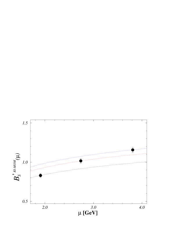
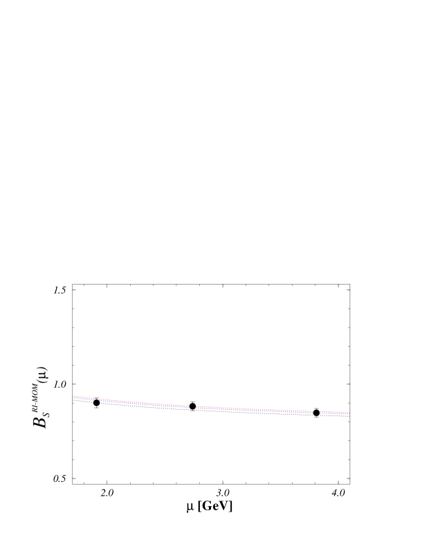
Figure 4: NLO evolution of the parameters ${B}^{\prime}_{S}(\mu)$ and ${B}_{S}(\mu)$ in the RI-MOM scheme. The curves are obtained by starting the evolution from the lattice results (filled circles) at $\mu=1.9$, $2.7$ and $3.8$ GeV, respectively.

From the figure, we see that $B_{S}^{\prime}(1.9\ {\rm GeV})$ falls below the other results. On the other hand, the evolution curves relative to $B_{S}^{\prime}(\mu=2.7\ {\rm GeV})$ and $B_{S}^{\prime}(\mu=3.8\ {\rm GeV})$ are closer to each other. This is to be contrasted to the situation for $B_{S}(\mu)$ where the scale dependence is not as large as for $B_{S}^{\prime}(\mu)$, and the description of our data by the perturbative NLO anomalous dimension is more satisfactory, as also shown in Fig. 4. To convert our result to the $\overline{\rm MS}$ scheme, as central values we choose the $B$-parameters obtained with the non-perturbative renormalization at $\mu=3.8$ GeV. The difference with the other results will be accounted in the systematic uncertainty.

3.2 $B$ parameters in the $\overline{\rm MS}$ scheme at $\mu=m_{b}$

In ref. [4], the formulae in eqs. (2) and (6) were derived in the $\overline{\rm MS}$ scheme. For this reason we have to convert our results from RI-MOM to $\overline{\rm MS}$. We have chosen to change renormalization scheme before extrapolating in the heavy quark mass. The change of scheme is obtained by using the relation

$$\langle\vec{Q}^{\overline{\rm MS}}(\mu)\rangle\ =\ \left(\widehat{1}\ +\ {r}_{\overline{\rm MS}}\ {\alpha_{s}(\mu)\over 4\pi}\right)\ \langle\vec{Q}^{\rm RI-MOM}(\mu)\rangle\;,$$

where

$$\quad\;{r}_{\overline{\rm MS}}\ =\ {1\over 18}\ \left(\begin{array}[]{cc}{\phantom{\Huge{l}}}\raisebox{-11.38092pt}{\phantom{\Huge{j}}}56+88\ \log 2&\;-8+56\ \log 2\\ {\phantom{\Huge{l}}}\raisebox{-11.38092pt}{\phantom{\Huge{j}}}-143+56\ \log 2&\;-115+88\ \log 2\\ \end{array}\right)\ .$$ (57)

We note that ${r}_{\overline{\rm MS}}$ is independent of $n_{f}$. $\langle\vec{Q}^{\overline{\rm MS}}(\mu=3.8{\rm GeV})\rangle$ is then evolved to $\mu=m_{b}=4.6$ GeV using (46), with ${J}_{\rm RI-MOM}^{n_{f}=0}$ replaced by

$$J^{n_{f}=0}_{\overline{\rm MS}}\ =\ \ \left(\begin{array}[]{cc}{\phantom{\Huge{l}}}\raisebox{-11.38092pt}{\phantom{\Huge{j}}}\frac{\large 9561}{3025}&\;-\frac{20723}{18150}\\ {\phantom{\Huge{l}}}\raisebox{-11.38092pt}{\phantom{\Huge{j}}}{{1811}\over{9075}}&\;-{{4997}\over{6050}}\\ \end{array}\right)\ .$$ (60)

The $\overline{\rm MS}$ $B$-parameters at $\mu=m_{b}^{\rm pole}=4.6$ GeV are presented in Tab. 5. $m_{b}^{\rm pole}=4.6$ GeV corresponds to the $\overline{\rm MS}$ mass given in Tab. 1 and it is very close to the value used in [4] to evaluate the Wilson coefficients at NLO.

lj $\kappa_{Q}$	0.1250		0.1220		0.1190
lj Light quark	$q=s$	$q=d$	$q=s$	$q=d$	$q=s$	$q=d$
lj $m_{P}$ [GeV]	1.85(7)	1.75(8)	2.11(9)	2.02(9)	2.38(10)	2.26(11)
lj $B_{S}^{\prime}(m_{P},m_{b})$	1.52(5)	1.60(8)	1.35(4)	1.39(7)	1.21(3)	1.25(5)
lj $\tilde{B}_{S}^{\prime}(m_{P},m_{b})$	2.18(8)	2.31(12)	1.93(6)	1.99(10)	1.72(5)	1.79(8)
lj $B_{S}(m_{P},m_{b})$	0.73(2)	0.71(3)	0.76(2)	0.72(3)	0.78(2)	0.76(3)
lj $\tilde{B}_{S}(m_{P},m_{b})$	1.05(3)	1.03(5)	1.08(3)	1.03(5)	1.10(3)	1.09(5)

Table 5: $B$-parameters in the $\overline{\rm MS}$ scheme at $\mu=4.6$ GeV.

3.3 Extrapolation to the $B_{s}$ meson

From Tabs. 3, 4 and 5, we observe that the dependence of $B_{S}^{\prime}$ on both the renormalization scale and the heavy-quark (meson) mass is much more pronounced than in the case of the parameter $B_{S}$ (see also Figs. 4 and 5). In particular, because of the large mass dependence, it is more difficult to extrapolate $B_{S}^{\prime}$ to the physical point. This is related to the fact that in eqs. (20) the ratio $(m_{B_{s}}/m_{b})^{2}$, distinguishing $B_{S}$ from $B^{\prime}_{S}$, still varies very rapidly in the mass range (around the charm) covered in our simulation. A similar problem is found if one tries to extract $m_{b}$ from the heavy-meson spectrum, computed with fully propagating quarks, by extrapolating in the heavy-quark mass. For this reason, so far, $m_{b}$ has been computed on the lattice only by using the Heavy Quark Effective Theory (HQET) [22] or Non-Relativistic QCD (NRQCD) [23]. Thus, although in principle we would prefer $B^{\prime}_{S}$ because it allows the evaluation of the matrix element without using the quark mass, in practice our best results are those obtained from $B_{S}$. For the same reasons, we were unable to extract ${\cal R}(m_{b})=\langle Q_{S}\rangle/\langle Q_{L}\rangle$ directly from the ratio of the matrix elements. The strongest dependence of $B^{\prime}_{S}$ on the quark mass finds its explanation in the framework of the HQET, by studying the leading and subleading contributions in the $1/m_{b}$ expansion to the $B$ parameters [24]. Our estimates of $\left(\Delta\Gamma_{B_{s}}/\Gamma_{B_{s}}\right)$ are then obtained with ${\cal R}(m_{b})$ computed by using $B_{S}$, $B_{B_{s}}$ and $m_{b}$ from Tab. 1, as shown below. For completeness we also present the results for $B^{\prime}_{S}$. Hopefully, when smaller values of the lattice spacing, and hence larger values of the heavy quark mass, will be accessible, an accurate determination of the physical matrix element will be provided by $B^{\prime}_{S}$.

In order to make the extrapolation in the heavy-quark mass from the region where we have data to $m_{b}$, we rely on the scaling laws of the HQET. The $B$-parameters in Tab. 5 have been obtained using the anomalous dimension matrix of the massless theory. This is the appropriate procedure since, on our data, $\mu$ is larger than the heavy quark mass, $m_{Q}$, used in our simulation. In order to use the HQET scaling laws, we have to evolve first to a scale smaller than the quark mass, at $m_{Q}$ fixed, and then to study the scaling at fixed $\mu$ as a function of the heavy quark mass. In practice, this is achieved, at LO in the anomalous dimensions, by introducing the following quantities:

$$\vec{\Phi}(m_{P_{s}},m_{b})=\left({\alpha_{s}(m_{P_{s}})\over\alpha_{s}(m_{B_{s}})}\right)^{\gamma/2\beta_{0}}\vec{B}(m_{P_{s}},m_{b})$$ (61)

(62)

$$\vec{\Phi}^{\prime}(m_{P_{s}},m_{b})=\left({\alpha_{s}(m_{P_{s}})\over\alpha_{s}(m_{B_{s}})}\right)^{\gamma^{\prime}/2\beta_{0}}\vec{B}^{\prime}(m_{P_{s}},m_{b})$$ (63)

where we have introduced the matrices $\gamma=\gamma_{0}-\widetilde{\gamma}_{0}+2(\widetilde{\gamma}_{P}-\gamma_{P})$, and $\gamma^{\prime}=\gamma_{0}-\widetilde{\gamma}_{0}+2\widetilde{\gamma}_{A}$. $\vec{B}=\left(B_{S},\tilde{B}_{S}\right)^{T}$ and similarly for $\vec{B}^{\prime}$. $\widetilde{\gamma}_{0}$ is the HQET anomalous dimension matrix which at leading order is given by

$$\widetilde{\gamma}_{0}\ =\ -{8\over 3}\ \left(\begin{array}[]{cc}2&\;1\\ 1&\;2\\ \end{array}\right)\ ,$$ (66)

whereas $\widetilde{\gamma}_{P}=\widetilde{\gamma}_{A}=-4$ and the LO anomalous dimension of the pseudoscalar density in full QCD is given by $\gamma_{P}=-8$.

The quantity $\vec{\Phi}(m_{P_{s}},m_{b})$ scales with the heavy quark (heavy meson) as:

$$\vec{\Phi}(m_{P_{s}},m_{b})\ =\ \alpha+{\beta\over m_{P_{s}}}+\dots$$ (67)

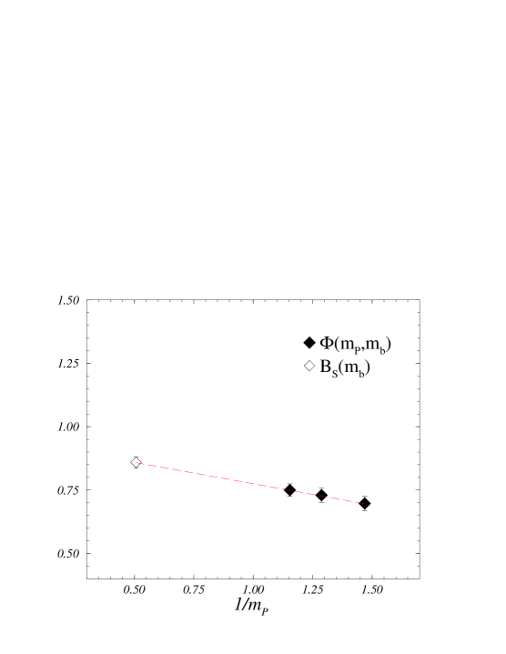
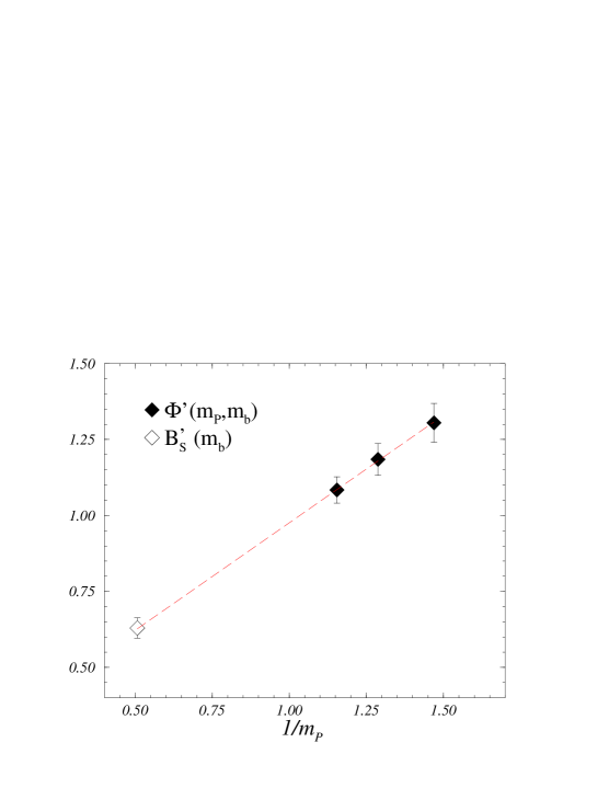
Figure 5: Extrapolation of $\Phi(m_{P},m_{b})$ and $\Phi^{\prime}(m_{P},m_{b})$ in $1/m_{P}$ to the $B_{s}$-meson mass. $m_{P}$ is given in lattice units.

The extrapolations of $B_{S}^{\overline{\rm MS}}(m_{b})$ and $B_{S}^{\prime\overline{\rm MS}}(m_{b})$ to $m_{B_{s}}$ are shown in Fig. 5. The results are:

$$B_{S}^{\overline{\rm MS}}(m_{b})=0.86(2)\;,\quad\tilde{B}_{S}^{\overline{\rm MS}}(m_{b})=1.25(3)$$ (68)

(69)

$$B_{S}^{\prime\ \overline{\rm MS}}(m_{b})=0.63(3)\;,\quad\tilde{B}_{S}^{\prime\ \overline{\rm MS}}(m_{b})=0.91(5)\;.$$ (70)

As for the systematic uncertainties, we account for the following two:

• if, instead of converting to the $\overline{\rm MS}$ scheme before extrapolating to $m_{B_{s}}$, we extrapolate our RI-MOM results (obtained at $\mu=3.8$ GeV) in the heavy quark by using the same scaling laws of eqs. (61), then evolve to $\mu=m_{b}$, and convert to the $\overline{\rm MS}$ scheme, the results are :

  $$B_{S}^{\overline{\rm MS}}(m_{b})=0.88(2)\;,\quad\tilde{B}_{S}^{\overline{\rm MS}}(m_{b})=1.27(3)$$ (71)

  (72)

  $$B_{S}^{\prime\ \overline{\rm MS}}(m_{b})=0.62(3)\;,\quad\tilde{B}_{S}^{\prime\ \overline{\rm MS}}(m_{b})=0.90(5)\;.$$ (73)

• if we start from a $\mu$ lower than $3.8$ GeV, for example $\mu=1.9$ GeV, then $B_{S}(m_{b})$ and $\tilde{B}_{S}(m_{b})$ change by $-3$%, while $B^{\prime}_{S}(m_{b})$ and $\tilde{B}^{\prime}_{S}(m_{b})$ drop by $-6$%.

After combining these uncertainties, we arrive at our final results:

$$B_{S}^{\overline{\rm MS}}(m_{b})=0.86(2)^{+0.02}_{-0.03}\;, \tilde{B}_{S}^{\overline{\rm MS}}(m_{b})=1.25(3)^{+0.02}_{-0.05}\;,$$ (74)

$$B_{S}^{\prime\ \overline{\rm MS}}(m_{b})=0.63(3)^{+0.00}_{-0.04}\;, \tilde{B}_{S}^{\prime\ \overline{\rm MS}}(m_{b})=0.91(5)^{+0.00}_{-0.06}\;.$$ (76)

From these numbers, we observe that there is a discrepancy between the value of $B_{S}^{\overline{\rm MS}}(m_{b})$ and $B_{S}^{\prime\ \overline{\rm MS}}(m_{b})$. Using $B_{S}^{\prime\ \overline{\rm MS}}(m_{b})\simeq(m_{B_{s}}/m_{b})^{2}B_{S}^{\overline{\rm MS}}(m_{b})$, with $(m_{B_{s}}/m_{b})^{2}=1.6$ from Tab. 1, we get $B_{S}^{\prime\ \overline{\rm MS}}(m_{b})\sim 1.37$, which is about twice the value of $B_{S}^{\prime\ \overline{\rm MS}}(m_{b})$ in (76).

In order to obtain the physical results we have used $B_{S}^{\overline{\rm MS}}(m_{b})$, for which the extrapolation to the $B_{s}$ meson is much smoother. In this case, we are obliged to use the quark mass to derive the matrix element needed to obtain ${\cal R}(m_{b})$, which is the relevant quantity for $\left(\Delta\Gamma_{B_{s}}/\Gamma_{B_{s}}\right)$, as explained in the introduction. This is not a major concern, however, since $m_{b}$ is known with a very tiny error (see Tab. 1).

The best way to minimize the statistical uncertainty is to compute on the same set of configurations

$${B_{S}^{\overline{\rm MS}}(m_{b})\over B_{B_{s}}^{\overline{\rm MS}}(m_{b})}=0.95(3)^{+0.00}_{-0.02}\ ,$$ (77)

which, when combined with the numbers from the Tab. 1, gives the wanted quantity

$${\cal R}(m_{b})=-{5\over 8}\left({m_{B_{s}}\over m_{b}(m_{b})+m_{s}(m_{b})}\right)^{2}{B_{S}(m_{b})\over B_{B_{s}}(m_{b})}=-0.93(3)^{+0.00}_{-0.01}\ .$$ (78)

4 Conclusion

In this section, we compare our results with previous lattice studies and draw our conclusion.

The first lattice calculation of $B_{S}(\mu)$ was performed in ref. [25], using the (unimproved) Wilson fermion action. Their $B$-parameters were obtained in a modified $\overline{\rm MS}$ NDR scheme, at the scale $\mu=2.33$ GeV, at a heavy-quark mass corresponding approximately to the $D_{s}$ mass. By translating their result to the $\overline{\rm MS}$ of ref. [6], one finds $B^{\overline{\rm MS}}_{S}(2.33\ {\rm GeV})=0.81(1)$ and $\tilde{B}^{\overline{\rm MS}}_{S}(2.33\ {\rm GeV})=0.86(1)$. To compare with these numbers, we have used our results at $\kappa_{Q}=0.1250$, interpolated to the strange light-quark mass and then evolved down to $\mu=2.33$ GeV. We get $B^{\overline{\rm MS}}_{S}(2.33\ {\rm GeV})=0.80(2)$ and $\tilde{B}^{\overline{\rm MS}}_{S}(2.33\ {\rm GeV})=1.05(2)$. $B^{\overline{\rm MS}}_{S}$ is hence in very good agreement with the value of [25], whereas our $\tilde{B}^{\overline{\rm MS}}_{S}$ is $20$% larger. We note, however, that the values $B^{\overline{\rm MS}}_{S}(2.33\ {\rm GeV})=0.81$ and $\tilde{B}^{\overline{\rm MS}}_{S}(2.33\ {\rm GeV})=0.86$ correspond (only evolution but no extrapolation in the heavy quark mass) to $B^{\overline{\rm MS}}_{S}(m_{b})=0.75$ [6] which is $14\%$ smaller than our number.

In refs. [17, 26], NRQCD has been used to compute $B^{\prime}_{S}(m_{b})$. A comparison with them is interesting, because effective theories have different systematic errors with respect to the approach followed in the present study. Their latest result (which we convert to $B_{S}$) reads $B^{\overline{\rm MS}}_{S}(m_{b})=0.78(2)(10)$, which is in fair agreement with ours. Moreover their ratio $B_{S}^{\overline{\rm MS}}(m_{b})/B_{B_{s}}^{\overline{\rm MS}}(m_{b})\sim 0.78/0.85=0.92$ is very close to ours. This implies that, in spite of the difference in the single $B$-parameters, the same physical answer for $\left(\Delta\Gamma_{B_{s}}/\Gamma_{B_{s}}\right)$ is obtained from eq. (10). In [17, 26], in order to get the width difference, they adopted, however, another expression (eq. (4) of [26]), which uses different inputs, namely the experimental inclusive semileptonic branching ratio and the theoretical determination of the decay constant $f_{B_{s}}=245\pm 30$ MeV. Their result [17], $\left(\Delta\Gamma_{B_{s}}/\Gamma_{B_{s}}\right)=(10.7\pm 2.6\pm 1.4\pm 1.7)\times 10^{-2}$ is about a factor of two larger than ours. One may wonder whether the difference is due to a different evaluation of the $1/m$ corrections, which are so important in this game. From our calculation, we find that this contribution to $\left(\Delta\Gamma_{B_{s}}/\Gamma_{B_{s}}\right)$ is about $-8.6\times 10^{-2}$, identical to the value used in [17] and [26] (eq. (9) of [26]). Besides the fact that they use a formula which involves the inclusive semileptonic branching ratio, the main difference stems, instead, from the use of a very large value of $f_{B_{s}}$ (and to a lesser extent from the use of $m_{b}=4.8$ GeV instead of $4.6$ GeV). We do not find it justified to use the unquenched value of $f_{B_{s}}$, combined with $B$ parameters computed in the quenched approximation. What really matters is the combination of these quantities in the matrix elements, and we do not know how much the $B$ parameters change in the unquenched case. This is the reason why we prefer eq. (10), which does not require $f_{B_{s}}$, but only ${\cal R}(m_{b})$ (which is essentially the same for us and in [17]) and $\xi$, which is known to remain almost the same in the quenched and unquenched case [10].

On the lattice, physical quantities relevant in heavy-quark physics can be computed following two main routes, either by extrapolating the results in the heavy-quark mass from a region around the charm mass or by using some effective theory (HQET or NRQCD). The two approaches have different systematics and in many cases lead to results which are barely compatible. The $B_{s}$ width difference is particularly lucky, in this respect, since ${\cal R}(m_{b})$ in our calculation and in ref. [17] are in excellent agreement and lead to the same value of $\left(\Delta\Gamma_{B_{s}}/\Gamma_{B_{s}}\right)$ if eq. (10) is used. It is not surprising that ref. [17] predicts a much larger value for $\left(\Delta\Gamma_{B_{s}}/\Gamma_{B_{s}}\right)$, since they use a very large value of $f_{B_{s}}$, which is not needed in eq. (10). We find that, in order to reduce the present error, a better determination of the $1/m$ correction, although rather hard, is very important. Obviously, calculations with larger heavy-quark masses and without quenching are also demanded for a better control of the remaining systematic errors.

References

- [1] R. Barate et al. [ALEPH Collaboration], CERN-EP-2000-036.
- [2] O. Schneider, talk given at “ Rencontres de Moriond” Les Arcs, France, 11-18 March 2000, [hep-ex/0006006].
- [3] V. A. Khoze, M. A. Shifman, N. G. Uraltsev and M. B. Voloshin, Sov. J. Nucl. Phys. 46 (1987) 112.
- [4] M. Beneke, G. Buchalla and I. Dunietz, Phys. Rev. D54 (1996) 4419 [hep-ph/9605259].
- [5] I. Dunietz, Eur. Phys. J. C7 (1999) 197 [hep-ph/9806521].
- [6] M. Beneke, G. Buchalla, C. Greub, A. Lenz and U. Nierste, Phys. Lett. B459 (1999) 631 [hep-ph/9808385].
- [7] A. J. Buras, M. Jamin and P. H. Weisz, Nucl. Phys. B347 (1990) 491.
- [8] T. Inami and C. S. Lim, Prog. Theor. Phys. 65 (1981) 297.
- [9] The LEP B Oscillation Working Group, LEPBOSC 98/3.
- [10] S. Hashimoto, review talk given at the 17th International Symposium on Lattice Field Theory “Lattice ’99”, Pisa, Italy, 29 Jun - 3 Jul 1999,[hep-lat/9909136].
- [11] D. Becirevic, D. Meloni, A. Retico, V. Gimenez, L. Giusti, V. Lubicz and G. Martinelli, [hep-lat/0002025].
- [12] M. Ciuchini, E. Franco, L. Giusti, V. Lubicz and G. Martinelli, Nucl. Phys. B573 (2000) 201 [hep-ph/9910236].
- [13] M. Lüscher, Les Houches Lectures on “Advanced Lattice QCD”, and refs. therein [hep-lat/9802029].
- [14] G. Martinelli, C. Pittori, C. T. Sachrajda, M. Testa and A. Vladikas, Nucl. Phys. B445 (1995) 81 [hep-lat/9411010].
- [15] A. Donini et al., Phys. Lett. B360 (1996) 83; M. Crisafulli et al., Phys. Lett. B369 (1996) 325; A. Donini et al., Phys.Lett. B470 (1999) 233, [hep-lat/9910017]; L. Conti et al., Phys.Lett. B421 (1998) 273, [hep-lat/9711053].
- [16] A. Donini, V. Gimenez, G. Martinelli, M. Talevi and A. Vladikas, Eur. Phys. J. C10 (1999) 121 [hep-lat/9902030].
- [17] S. Hashimoto, K. I. Ishikawa, T. Onogi, M. Sakamoto, N. Tsutsui and N. Yamada, [hep-lat/0004022].
- [18] D. Becirevic, P. Boucaud, V. Gimenez, V. Lubicz, G. Martinelli, J. Micheli and M. Papinutto, [hep-lat/0005013].
- [19] A. Donini, V. Gimenez, L. Giusti and G. Martinelli, Phys. Lett. B470 (1999) 233 [hep-lat/9910017].
- [20] M. Ciuchini, E. Franco, V. Lubicz, G. Martinelli, I. Scimemi and L. Silvestrini, Nucl. Phys. B523 (1998) 501 [hep-ph/9711402].
- [21] A. J. Buras, M. Misiak and J. Urban, [hep-ph/0005183].
- [22] V. Gimenez, G. Martinelli and C. T. Sachrajda, Phys. Lett. B393 (1997) 124 [hep-lat/9607018]; G. Martinelli and C. T. Sachrajda, Nucl. Phys. B559 (1999) 429 [hep-lat/9812001]; V. Gimenez, L. Giusti, G. Martinelli and F. Rapuano, JHEP 0003 (2000) 018 [hep-lat/0002007].
- [23] C. T. Davies et al., Phys. Rev. Lett. 73 (1994) 2654 [hep-lat/9404012]; A. Ali Khan et al., [hep-lat/9912034].
- [24] V. Gimenez and J. Reyes, in preparation.
- [25] R. Gupta, T. Bhattacharya and S. Sharpe, Phys. Rev. D55 (1997) 4036 [hep-lat/9611023].
- [26] S. Hashimoto, K. I. Ishikawa, T. Onogi and N. Yamada, [hep-ph/9912318].