QCD factorization for exclusive non-leptonic

$B$-meson decays: General arguments

and the case of heavy–light final states

M. Beneke^a, G. Buchalla^b, M. Neubert^c and C.T. Sachrajda^d

^aInstitut für Theoretische Physik E, RWTH Aachen

D - 52056 Aachen, Germany

^bTheory Division, CERN, CH-1211 Geneva 23, Switzerland

^cNewman Laboratory of Nuclear Studies

Cornell University, Ithaca, NY 14853, USA

^dDepartment of Physics and Astronomy, University of Southampton

Southampton SO17 1BJ, UK

Abstract

We provide a rigorous basis for factorization for a large class of non-leptonic two-body $B$-meson decays in the heavy-quark limit. The resulting factorization formula incorporates elements of the naive factorization approach and the hard-scattering approach, but allows us to compute systematically radiative (“non-factorizable”) corrections to naive factorization for decays such as $B\to D\pi$ and $B\to\pi\pi$. We first discuss the factorization formula from a general point of view. We then consider factorization for decays into heavy-light final states (such as $B\to D\pi$) in more detail, including a proof of the factorization formula at two-loop order. Explicit results for the leading QCD corrections to factorization are presented and compared to existing measurements of branching fractions and final-state interaction phases.

1 Introduction

Non-leptonic, two-body $B$-meson decays, although simple as far as the underlying weak decay of the $b$ quark is concerned, are complicated on account of strong-interaction effects. If these effects could be computed, this would enhance tremendously our ability to uncover the origin of CP violation in weak interactions from data on a variety of such decays being collected at the $B$ factories.

In this paper we begin a systematic analysis of weak heavy-meson decays into two energetic mesons based on the factorization properties of decay amplitudes in quantum chromodynamics (QCD). (Some of the results have already been presented in [1].) As in the classic analysis of semi-leptonic $B\to D$ transitions [2, 3], our arguments make extensive use of the fact that the $b$ quark is heavy compared to the intrinsic scale of strong interactions. This allows us to deduce that non-leptonic decay amplitudes in the heavy-quark limit have a simple structure. The arguments to reach this conclusion, however, are quite different from those used for semi-leptonic decays, since for non-leptonic decays a large momentum is transferred to at least one of the final-state mesons. The results of this work justify naive factorization of four fermion operators for many, but not all, non-leptonic decays and imply that corrections termed “non-factorizable”, which up to now have been thought to be intractable, can be calculated rigorously, if the mass of the weakly decaying quark is large enough. This leads to a large number of predictions for CP-violating $B$ decays in the heavy-quark limit, for which measurements will soon become available.

Weak decays of heavy mesons involve three fundamental scales, the weak interaction scale $M_{W}$, the $b$-quark mass $m_{b}$, and the QCD scale $\Lambda_{\rm QCD}$, which are strongly ordered: $M_{W}\gg m_{b}\gg\Lambda_{\rm QCD}$. The underlying weak decay being computable, all theoretical work concerns strong-interaction corrections. The strong-interaction effects which involve virtualities above the scale $m_{b}$ are well understood. They renormalize the coefficients of local operators ${\cal O}_{i}$ in the weak effective Hamiltonian [4], so that the amplitude for the decay $B\to M_{1}M_{2}$ is given by

$${\cal A}(B\to M_{1}M_{2})=\frac{G_{F}}{\sqrt{2}}\sum_{i}\lambda_{i}\,C_{i}(\mu)\,\langle M_{1}M_{2}|{\cal O}_{i}|B\rangle(\mu),$$ (1)

where $G_{F}$ is the Fermi constant. Each term in the sum is the product of a Cabibbo-Kobayashi-Maskawa (CKM) factor $\lambda_{i}$, a coefficient function $C_{i}(\mu)$, which incorporates strong-interaction effects above the scale $\mu\sim m_{b}$, and a matrix element of an operator ${\cal O}_{i}$. The most difficult theoretical problem is to compute these matrix elements or, at least, to reduce them to simpler non-perturbative objects.

There exist a variety of treatments of this problem, on many of which we will comment later, which rely on assumptions of some sort. Here we identify two somewhat contrary lines of approach. (A more comprehensive discussion of the literature on non-leptonic $B$ decays is given in a separate section of this paper.)

The first approach, which we shall call “naive factorization”, replaces the matrix element of a four-fermion operator in a heavy-quark decay by the product of the matrix elements of two currents [5, 6], for example,

$$\langle\pi^{+}\pi^{-}|(\bar{u}b)_{\rm V-A}(\bar{d}u)_{\rm V-A}|\bar{B}_{d}\rangle\to\langle\pi^{-}|(\bar{d}u)_{\rm V-A}|0\rangle\,\langle\pi^{+}|(\bar{u}b)_{\rm V-A}|\bar{B}_{d}\rangle.$$ (2)

This assumes that the exchange of “non-factorizable” gluons between the $\pi^{-}$ and the $(\bar{B_{d}}\,\pi^{+})$ system can be neglected, if the virtuality of the gluons is below $\mu\sim m_{b}$. The non-leptonic decay amplitude reduces to the product of a form factor and a decay constant. This assumption is in general not justified, except in the limit of a large number of colours in some cases. It deprives the amplitude of any physical mechanism that could account for rescattering in the final state and for the generation of a strong phase shift between different amplitudes. “Non-factorizable” radiative corrections must also exist, because the scale dependence of the two sides of (2) is different. Since “non-factorizable” corrections at scales larger than $\mu$ are taken into account in deriving the effective weak Hamiltonian, it appears rather arbitrary to leave them out below the scale $\mu$.

The correct scale dependence can be restored by computing the transition matrix element for an inclusive or partonic final state and by absorbing the correction into effective scale-independent coefficients. However, without a systematic approach to computing the hadronic matrix elements, this sidelines the real question of how to improve the parametric accuracy of the naive factorization approach.

Various generalizations of the naive factorization approach have been proposed, which include new parameters that account for non-factorizable corrections. In the most general form, these generalizations have nothing to do with the original “factorization” ansatz, but amount to a general parameterization of the matrix elements, including those of penguin operators. Such general parameterizations are exact, but at the price of introducing many unknown parameters and eliminating any theoretical input on strong-interaction dynamics. Making such a parameterization useful requires certain assumptions that relate these parameters.

The second method used to study non-leptonic decays is the hard-scattering approach. Here the assumption is that the decay is dominated by hard gluon exchange. The decay amplitude is then expressed as a convolution of a hard-scattering factor with light-cone wave functions of the participating mesons, for example,

$$\langle\pi^{+}\pi^{-}|(\bar{u}b)_{\rm V-A}(\bar{d}u)_{\rm V-A}|\bar{B}_{d}\rangle\to\int_{0}^{1}\!d\xi dudv\,\Phi_{B}(\xi)\,\Phi_{\pi}(u)\,\Phi_{\pi}(v)\,T(\xi,u,v;m_{b}).$$ (3)

This is analogous to more familiar applications of this method to hard exclusive reactions involving only light hadrons [7, 8].

For many hard exclusive processes the hard-scattering contribution represents the leading term in an expansion in $\Lambda_{\rm QCD}/Q$, where $Q$ denotes the hard scale. However, the short-distance dominance of hard exclusive processes is not enforced kinematically and relies crucially on the properties of hadronic wave functions. There is an important difference between light mesons and heavy mesons regarding these wave functions, because the light quark in a heavy meson at rest naturally has a small momentum of order $\Lambda_{\rm QCD}$, while for fast light mesons a configuration with a soft quark is suppressed by the meson’s wave function. As a consequence the soft (or Feynman) mechanism is power suppressed for hard exclusive processes involving light mesons, but it is of leading power, and in fact larger than the hard-scattering contribution by a factor $1/\alpha_{s}(\sqrt{m_{b}\Lambda_{\rm QCD}})$, for heavy-meson decays. (The arguments that lead to this conclusion will be reviewed below.)

A standard analysis of higher-order corrections to the hard-scattering amplitude $T$ in (3) shows that the configuration in which the final-state meson picks up the soft spectator quark of the heavy meson as a soft quark is suppressed by a Sudakov form factor, if the meson has large momentum. This suggests that the hard-scattering term may become dominant even for heavy-meson decays, if the heavy-quark mass is very large. However, calculation of the $B\to\pi$ form factors in the QCD sum rule approach [9, 10] indicates that the soft contribution dominates for $b$ quarks with $m_{b}\approx 5\,$GeV. Even if Sudakov suppression were effective, arguing away the soft contribution in this way is not completely satisfactory; a factorization formula that separates soft and hard contributions on the basis of power counting alone is more desirable.

It is clear from this discussion that a satisfactory treatment should take into account soft contributions (and hence provide the correct asymptotic limit – if we ignore Sudakov suppression factors), but also allow us to compute corrections to the naive factorization result in a systematic way (and hence result in a scheme- and scale-independent expression up to corrections of higher order in the strong coupling $\alpha_{s}$).

It is not at all obvious that such a treatment would result in a predictive framework. We will show that this does indeed happen for most non-leptonic two-body $B$ decays. Our main conclusion is that “non-factorizable” corrections are dominated by hard gluon exchange, while the soft effects that survive in the heavy-quark limit are confined to the $(BM_{1})$ system, where $M_{1}$ denotes the meson that picks up the spectator quark in the $B$ meson. This result is expressed as a factorization formula, which is valid up to corrections suppressed by $\Lambda_{\rm QCD}/m_{b}$. At leading power non-perturbative contributions are parameterized by the physical form factors for the $B\to M_{1}$ transition and leading-twist light-cone distribution amplitudes of the mesons. Hard perturbative corrections can be computed systematically in a way similar to the hard-scattering approach. On the other hand, because the $B\to M_{1}$ transition is parameterized by a form factor, we recover the result of naive factorization at lowest order in $\alpha_{s}$. An important implication of the factorization formula is that strong rescattering phases are either perturbative or power suppressed in $m_{b}$. It is worth emphasizing that the decoupling of $M_{2}$ occurs in the presence of soft interactions in the $(BM_{1})$ system. In other words, while strong-interaction effects in the $B\to M_{1}$ transition are not confined to small transverse distances, the other meson $M_{2}$ is predominantly produced as a compact object with small transverse extension. The decoupling of soft effects then follows from “colour transparency”. The colour-transparency argument for exclusive $B$ decays has already been noted in the literature [11, 12], but it has never been developed into a factorization formula that could be used to obtain quantitative predictions.

The approach described in this paper is general and applies to decays into a heavy and a light meson (such as $B\to D\pi$) as well as to decays into two light mesons (such as $B\to\pi\pi$, $B\to\pi K$, etc.). Factorization does not hold, however, for decays such as $B\to\pi D$ and $B\to DD_{s}$, in which the meson that does not pick up the spectator quark in the $B$ meson is heavy. For the special case of the ratio $\Gamma(B\to D^{*}\pi)/\Gamma(B\to D\pi)$ Politzer and Wise evaluated “non-factorizable” one-loop corrections several years ago [13]. Their result agrees with the result obtained from the general factorization formula proposed here.

The outline of the paper is as follows: in Sect. 2 we state the factorization formula in its general form and define the various elements of the formula, in particular the light-cone distribution amplitudes. In Sect. 3 we collect the arguments that lead to the factorization formula. We show how light-cone distribution amplitudes enter, discuss the heavy-quark scaling of the $B\to\pi$ form factor and the cancellation of soft and collinear effects. We also address the issue of multi-particle Fock states and annihilation topologies, which are power suppressed in $\Lambda_{\rm QCD}/m_{b}$. The arguments of this section are appropriate for decays into a heavy and a light meson, as well as, with some modifications, to decays into two light mesons. However, we will keep the discussion qualitative and leave technical details to later sections. In Sect. 4 we discuss the cancellation of long-distance singularities at one-loop order, and present the calculation of the hard-scattering functions at this order for decays into a heavy and a light meson. Sect. 5 extends the proof of the cancellation of singularities to two-loop order and provides arguments for factorization to all orders. In Sect. 6 we consider the phenomenology of decays into a heavy and a light meson on the basis of the factorization formula. We examine to what extent a charm meson should be considered as heavy or light and discuss various tests of the theoretical framework. A critical review of and comparison with other approaches to exclusive non-leptonic decays is given in Sect. 7. Sect. 8 contains our conclusion.

Except for the general discussion, we restrict this paper to the proof of factorization and the phenomenology for decays into a heavy and a light meson. The more elaborate technical arguments needed to establish the factorization formula for decays into two light mesons, together with an adequate discussion of the heavy-quark limit in this case, will be given in a subsequent paper.

2 Statement of the factorization formula

In this section we summarize the main result of this paper, the factorization formula for non-leptonic $B$ decays. We introduce relevant terminology and definitions.

2.1 The idea of factorization

In the context of non-leptonic decays the term “factorization” is usually applied to the approximation of the matrix element of a four fermion operator by the product of a form factor and a decay constant, see (2). Corrections to this approximation are called “non-factorizable”. We will refer to this approximation as “naive factorization” and use quotes on “non-factorizable” to avoid confusion with the meaning of factorization in the context of hard processes in QCD.

In the latter context factorization refers to the separation of long-distance contributions to the process from a short-distance part that depends only on the large scale $m_{b}$. The short-distance part can be computed in an expansion in the strong coupling $\alpha_{s}(m_{b})$. The long-distance contributions must be computed non-perturbatively or determined experimentally. The advantage is that these non-perturbative parameters are often simpler in structure than the original quantity, or they are process independent. For example, factorization applied to hard processes in inclusive hadron-hadron collisions requires only parton distributions as non-perturbative inputs. Parton distributions are much simpler objects than the original matrix element with two hadrons in the initial state. On the other hand, factorization applied to the $B\to D$ form factor leads to a non-perturbative object (the “Isgur-Wise function”) which is still a function of the momentum transfer. However, the benefit here is that symmetries relate this function to other form factors. In the case of non-leptonic $B$ decays, the simplification is primarily of the first kind (simpler structure). We call those effects non-factorizable (without quotes) which depend on the long-distance properties of the $B$ meson and both final-state mesons combined.

The factorization properties of non-leptonic decay amplitudes depend on the two-meson final state. We call a meson “light”, if its mass $m$ remains finite in the heavy-quark limit. A meson is called “heavy”, if we assume that its mass scales with $m_{b}$ in the heavy-quark limit, such that $m/m_{b}$ stays fixed. In principle, we could still have $m\gg\Lambda_{\rm QCD}$ for a light meson. Charm mesons could be considered as light in this sense. However, unless otherwise mentioned, we assume that $m$ is of order $\Lambda_{\rm QCD}$ for a light meson, and we consider charm mesons as heavy. We also restrict the term “heavy mesons” to mesons of a heavy and a light quark and do not include onia of two heavy quarks. The difference is that heavy and light mesons have large transverse extension of order $1/\Lambda_{\rm QCD}$, while the transverse size of onia becomes small in the heavy-quark limit.

Although not necessary, it is useful to describe non-leptonic decays in the $B$-meson rest frame. In this paper quantities which are not Lorentz invariant will always refer to this frame. In evaluating the scaling behaviour of the decay amplitudes we assume that the energies of both final-state mesons scale like $m_{b}$ in the heavy-quark limit. We do not consider explicitly the so-called small velocity limit for heavy mesons in which $m_{b}\sim m$ while $m_{b}-m\gg\Lambda_{\rm QCD}$ stays fixed in the heavy-quark limit, which implies $m/m_{b}\to 1$. Although our results remain valid in this limit, the assumption that $m/m_{b}$ stays fixed simplifies the discussion, because we do not have to distinguish the scales $m_{b}$ and $m_{b}-m$.

2.2 The factorization formula

We consider weak decays $B\to M_{1}M_{2}$ in the heavy-quark limit and differentiate between decays into final states containing a heavy and a light meson or two light mesons. Up to power corrections of order $\Lambda_{\rm QCD}/m_{b}$ the transition matrix element of an operator ${\cal O}_{i}$ in the weak effective Hamiltonian is given by

$$\langle M_{1}M_{2}|{\cal O}_{i}|\bar{B}\rangle = \sum_{j}F_{j}^{B\to M_{1}}(m_{2}^{2})\,\int_{0}^{1}du\,T_{ij}^{I}(u)\,\Phi_{M_{2}}(u)\,\,+\,\,(M_{1}\leftrightarrow M_{2})$$ (4)

$$+\,\int_{0}^{1}d\xi dudv\,T_{i}^{II}(\xi,u,v)\,\Phi_{B}(\xi)\,\Phi_{M_{1}}(v)\,\Phi_{M_{2}}(u)$$

if $$M_{1} M_{2}$$ and are both light,

$$\langle M_{1}M_{2}|{\cal O}_{i}|\bar{B}\rangle = \sum_{j}F_{j}^{B\to M_{1}}(m_{2}^{2})\,\int_{0}^{1}du\,T_{ij}^{I}(u)\,\Phi_{M_{2}}(u)$$

if $$M_{1} M_{2}$$ is heavy and is light.

Here $F_{j}^{B\to M_{1,2}}(m_{2,1}^{2})$ denotes a $B\to M_{1,2}$ form factor, and $\Phi_{X}(u)$ is the light-cone distribution amplitude for the quark-antiquark Fock state of meson $X$. These non-perturbative quantities will be defined precisely in the next subsection. $T_{ij}^{I}(u)$ and $T_{i}^{II}(\xi,u,v)$ are hard-scattering functions, which are perturbatively calculable. The hard-scattering kernels and light-cone distribution amplitudes depend on a factorization scale and scheme, which is suppressed in the notation of (4). Finally, $m_{1,2}$ denote the light meson masses. Eq. (4) is represented graphically in Fig. 1. (The second line of the first equation in (4) is somewhat simplified and may require including an integration over transverse momentum in the $B$ meson starting from order $\alpha_{s}^{2}$, see the remarks after (12).)

Figure 1: Graphical representation of the factorization formula. Only one of the two form-factor terms in (4) is shown for simplicity.

As it stands, the first equation in (4) applies to decays into two light mesons, for which the spectator quark in the $B$ meson (in the following simply referred to as the “spectator quark”) can go to either of the final-state mesons. An example is the decay $B^{-}\to\pi^{0}K^{-}$. If the spectator quark can go only to one of the final-state mesons, as for example in $\bar{B}_{d}\to\pi^{+}K^{-}$, we call this meson $M_{1}$ and the second form-factor term on the right-hand side of (4) is absent.

The factorization formula simplifies when the spectator quark goes to a heavy meson (second equation in (4)), such as in $\bar{B}_{d}\to D^{+}\pi^{-}$. In this case the third term on the right-hand side of (4), which accounts for hard interactions with the spectator quark, can be dropped because it is power suppressed in the heavy-quark limit. In the opposite situation that the spectator quark goes to a light meson but the other meson is heavy, factorization does not hold because the heavy meson is neither fast nor small and cannot be factorized from the $B\to M_{1}$ transition. However, such amplitudes are again power suppressed in the heavy-quark limit relative to amplitudes in which the spectator quark goes to a heavy meson while the other meson is light. (These statements will be justified in detail in Sect. 3.) We also note that factorization does hold, at least formally, if the emission particle $M_{2}$ is an onium. Finally, notice that annihilation topologies do not appear in the factorization formula. They do not contribute at leading order in the heavy-quark expansion.

Any hard interaction costs a power of $\alpha_{s}$. As a consequence the third term in (4) is absent at order $\alpha_{s}^{0}$. Since at this order the functions $T^{I}_{ij}(u)$ are independent of $u$, the convolution integral results in a meson decay constant and we see that (4) reproduces naive factorization. The factorization formula allows us to compute radiative corrections to this result to all orders in $\alpha_{s}$. Further corrections are suppressed by powers of $\Lambda_{\rm QCD}/m_{b}$ in the heavy-quark limit.

The significance and usefulness of the factorization formula stems from the fact that the non-perturbative quantities which appear on the right-hand side of (4) are much simpler than the original non-leptonic matrix element on the left-hand side. This is because they either reflect universal properties of a single meson state (light-cone distribution amplitudes) or refer only to a $B\to\mbox{meson}$ transition matrix element of a local current (form factors). While it is extremely difficult, if not impossible [14], to compute the original matrix element $\langle M_{1}M_{2}|{\cal O}_{i}|\bar{B}\rangle$ in lattice QCD, form factors and light-cone distribution amplitudes are already being computed in this way, although with significant systematic errors at present. Alternatively, form factors can be obtained using data on semi-leptonic decays, and light-cone distribution amplitudes by comparison with other hard exclusive processes.

Adopting the terminology introduced earlier, Eq. (4) implies that there exist no non-factorizable effects (in the sense of QCD factorization) at leading order in the heavy-quark expansion. Since the form factors and light-cone distribution amplitudes are real, all final-state interactions and the strong phases generated by them are part of the calculable hard-scattering functions. This and the absence of non-factorizable corrections is unlikely to be true beyond leading order in the heavy-quark expansion, because there exist soft gluon effects that connect $M_{1}$ and $M_{2}$, which are suppressed by one power of $\Lambda_{\rm QCD}/m_{b}$.

2.3 Definition of non-perturbative parameters

2.3.1 Form factors

The form factors $F_{j}^{B\to M}(q^{2})$ in (4) arise in the decomposition of matrix elements of the form

$$\langle M(p^{\prime})|\bar{q}\Gamma b|\bar{B}(p)\rangle,$$ (5)

where $\Gamma$ can be any irreducible Dirac matrix that appears after contraction of the hard subgraph to a local vertex with respect to the $B\to M$ transition. For the purpose of discussion we will often refer to the matrix element of the vector current, which is conventionally parameterized by two scalar form factors:

$$\langle P(p^{\prime})|\bar{q}\gamma^{\mu}b|\bar{B}(p)\rangle=F_{+}^{B\to P}(q^{2})\,(p^{\mu}+{p^{\prime}}^{\mu})+\Big{[}F_{0}^{B\to P}(q^{2})-F_{+}^{B\to P}(q^{2})\Big{]}\,\frac{m_{B}^{2}-m_{P}^{2}}{q^{2}}\,q^{\mu},$$ (6)

where $q=p-p^{\prime}$. The pseudoscalar meson is denoted by $P$, $m_{P}$ is its mass and $m_{B}$ the mass of the $B$ meson. For $q^{2}=0$ the two form factors coincide, $F_{+}^{B\to P}(0)=F_{0}^{B\to P}(0)$. The scaling of $F_{+}^{B\to P}(0)$ with $m_{b}$ will be discussed in Sect. 3.

Note that we write (4) in terms of physical form factors. In principle, Fig. 1 could be looked upon in two different ways. In the first way, we suppose that the region represented by ‘$F$’ accounts only for the soft contributions to the $B\to M_{1}$ form factor. The hard contributions to the form factor can be considered as part of $T^{I}_{ij}$ or as part of the second diagram, i.e. as part of the hard-scattering factor $T^{II}_{i}$. Performing this split-up requires that one understands the factorization of hard and soft contributions to the form factor. If $M_{1}$ is heavy, this amounts to matching the form factor onto a form factor defined in heavy-quark effective theory. However, for a light meson $M_{1}$, the factorization of hard and soft contributions to the form factor is not yet completely understood. We bypass this problem by interpreting ‘$F$’ as the physical form factor, including hard and soft contributions. The hard contributions to the form factor should then be omitted from the hard-scattering kernel $T^{II}_{i}$ and a subtraction has to be performed in $T^{I}_{ij}$ beginning at two-loop order (see also Sect. 5). The relevant diagrams are easily identified. An additional advantage of using physical form factors is that they are directly related to measurable quantities, or to the form factors obtained from lattice QCD or QCD sum rules.

2.3.2 Light-cone distribution amplitudes of light mesons

Light-cone distribution amplitudes play the same role for hard exclusive processes that parton distributions play for inclusive processes. As in the latter case, the leading-twist distribution amplitudes, which are the ones we need at leading power in the $1/m_{b}$ expansion, are given by two-particle operators with a certain helicity structure. The helicity structure is determined by the angular momentum of the meson and the fact that the spinor of an energetic quark has only two large components.

The leading-twist light-cone distribution amplitudes for pseudoscalar mesons ($P$), longitudinally polarized vector mesons ($V_{||}$), and transversely polarized vector mesons ($V_{\perp}$) with flavour content $(\bar{q}q^{\prime})$ are

$$\langle P(q)|\bar{q}(y)_{\alpha}q^{\prime}(x)_{\beta}|0\rangle\Big{|}_{(x-y)^{2}=0} = \frac{if_{P}}{4}\,(\not\!q\gamma_{5})_{\beta\alpha}\,\int_{0}^{1}du\,e^{i(\bar{u}qx+uqy)}\,\Phi_{P}(u,\mu),$$

$$\langle V_{||}(q)|\bar{q}(y)_{\alpha}q^{\prime}(x)_{\beta}|0\rangle\Big{|}_{(x-y)^{2}=0} = -\frac{if_{V}}{4}\!\!\not\!q_{\beta\alpha}\,\int_{0}^{1}du\,e^{i(\bar{u}qx+uqy)}\,\Phi_{||}(u,\mu),$$ (7)

$$\langle V_{\perp}(q)|\bar{q}(y)_{\alpha}q^{\prime}(x)_{\beta}|0\rangle\Big{|}_{(x-y)^{2}=0} = -\frac{if_{T}(\mu)}{8}\,[\not\!\varepsilon^{*}_{\perp},\not\!q\,]_{\beta\alpha}\,\int_{0}^{1}du\,e^{i(\bar{u}qx+uqy)}\,\Phi_{\perp}(u,\mu).$$

The equality sign is to be understood as “equal up to higher-twist terms”, and it is also understood that the operator on the left-hand side is a colour singlet. We use the “bar”-notation throughout this paper, i.e. $\bar{v}\equiv 1-v$ for any longitudinal momentum fraction variable. The parameter $\mu$ is the renormalization scale of the light-cone operators on the left-hand side. The distribution amplitudes are normalized as $\int_{0}^{1}du\,\Phi_{X}(u,\mu)=1$ $(X=P,||,\perp)$. One defines the asymptotic distribution amplitude as the limit in which the renormalization scale is sent to infinity. All three distribution amplitudes introduced above have the same asymptotic form

$$\Phi_{X}(u,\mu)\stackrel{{\scriptstyle\mu\to\infty}}{{=}}6u\bar{u}.$$ (8)

The decay constants appearing in (2.3.2) refer to the normalization in which $f_{\pi}=131\,$MeV. ($f_{T}(\mu)$ is scale dependent, because it is related to the matrix element of the non-conserved tensor current.) $\varepsilon_{\perp}^{\mu}$ is the polarization vector of a transversely polarized vector meson. For longitudinally polarized vector mesons we can identify $\varepsilon_{||}^{\mu}=q^{\mu}/m_{V}$, where $m_{V}$ is the vector-meson mass. Corrections to this are suppressed by two powers of $m_{V}/q^{0}\sim\Lambda_{\rm QCD}/m_{b}$. We have used this fact to eliminate the polarization vector of $V_{||}$ in (2.3.2). There is a path-ordered exponential that connects the two quark fields at different positions and makes the light-cone operators gauge invariant. In (2.3.2) we have suppressed this standard factor.

The use of light-cone distribution amplitudes in non-leptonic $B$ decays requires justification, which we will provide in Sect. 3. The decay amplitude is then calculated as follows: assign momentum $uq$ to the quark in the outgoing (light) meson with momentum $q$ and assign momentum $\bar{u}q$ to the antiquark. Write down the on-shell amplitude in momentum space with outgoing quark and antiquark of momentum $uq$ and $\bar{u}q$, respectively, and perform the replacement

$$\bar{u}_{\alpha a}(uq)\Gamma(u,\ldots)_{\alpha\beta,ab,\ldots}v_{\beta b}(\bar{u}q)\,\longrightarrow\,\frac{if_{P}}{4N_{c}}\int_{0}^{1}du\,\Phi_{P}(u)\,(\not\!q\gamma_{5})_{\beta\alpha}\Gamma(u,\ldots)_{\alpha\beta,aa,\ldots}$$ (9)

for pseudoscalars and, with obvious modifications, for vector mesons. (Here $N_{c}=3$ refers to the number of colours.)

Even when working with light-cone distribution amplitudes (light-cone wave functions integrated over transverse momentum) it is not always justified to perform the collinear approximation on the external quark (antiquark) lines right away. One may have to keep the transverse components of the quark momentum $k$ and be allowed to put $k=uq$ only after some operations on the amplitude have been carried out. However, these subtleties do not concern calculations that use only leading-twist light-cone distributions.

2.3.3 Light-cone distribution amplitudes of $B$ mesons

It is intuitive that light-cone distribution amplitudes for light mesons appear in non-leptonic decays. The relevance of light-cone distribution amplitudes of $B$ mesons is less clear, because the spectator quark in the $B$ meson is not energetic in the $B$-meson rest frame. Hence if we assign momentum $l$ to the spectator quark, all components of $l$ are of order $\Lambda_{\rm QCD}$.

The $B$-meson light-cone distribution amplitude appears only in the third term on the right-hand side of (4), the hard spectator interaction term. As discussed above, this term is of leading power only for decays into two light mesons or decays into a light meson and an onium. One finds, at least at order $\alpha_{s}$, that the hard spectator interaction amplitude depends only on $p^{\prime}\!\cdot l$ at leading order in $1/m_{b}$, where $p^{\prime}$ is the momentum of the light meson that picks up the spectator quark. We introduce light-cone components

$$v_{\pm}=\frac{v^{0}\pm v^{3}}{\sqrt{2}}$$ (10)

for any vector $v$. If we choose $p^{\prime}$ such that only $p^{\prime}_{-}$ is non-zero, the hard spectator amplitude $A(l,\ldots)$ depends only on $l_{+}$. The decay amplitude for the general two-particle Fock state of the $B$ meson is given by the integral over the full Bethe-Salpeter wave function

$$\Psi_{B}(z,p)=\langle 0|\bar{q}_{\alpha}(z)[\ldots]b_{\beta}(0)|\bar{B}_{d}(p)\rangle=\int\frac{d^{4}l}{(2\pi)^{4}}\,e^{-ilz}\,\hat{\Psi}_{B}(l,p)$$ (11)

with the partonic decay amplitude. (The dots denote the path-ordered exponential required to make the matrix element gauge invariant.) We then approximate

$$\int\frac{d^{4}l}{(2\pi)^{4}}\,A(l,\ldots)\,\hat{\Psi}_{B}(l,p)=\int dl_{+}\,A(l_{+},\ldots)\,\int\frac{d^{2}l_{\perp}dl_{-}}{(2\pi)^{4}}\,\hat{\Psi}_{B}(l,p),$$ (12)

which is valid up to power corrections. Since the wave function can be integrated over $l_{\perp}$ and $l_{-}$ it follows that we need $\Psi(z,p)$ only for light-like $z$, i.e. for $z_{+}=z_{\perp}=0$. We used this property to express the hard spectator interaction in (4) in terms of an integral over longitudinal momentum fraction $\xi$. It is possible that this cannot be justified in higher orders in perturbation theory. If not, the hard spectator interaction has to be generalized to include an integration over the transverse momentum. We leave this issue to subsequent work on factorization in decays into two light mesons. (An example for which this generalization is necessary is the decay $B^{+}\to\gamma e^{+}\nu$, which has recently been discussed in [15].) The qualitative discussion for light-light final states in this paper is not affected by this potential complication.

For the most general decomposition of the light-cone distribution amplitude at leading order in $1/m_{b}$, we make use of the fact that in the $B$-meson rest frame only the upper two components of the $b$-quark spinor are large. However, since the spectator quark is neither energetic nor heavy, no further restriction on the components of the spectator-quark spinor exists. We then find that the $B$ meson is described by two scalar wave functions at leading power, which we can choose as

$$\langle 0|\bar{q}_{\alpha}(z)[\ldots]b_{\beta}(0)|\bar{B}_{d}(p)\rangle\Big{|}_{z_{+}=z_{\perp}=0} =$$ (13)

$$-\frac{if_{B}}{4}\,[(\not\!p+m_{b})\gamma_{5}]_{\beta\gamma}\,\int_{0}^{1}d\xi\,e^{-i\xi p_{+}z_{-}}\left[\Phi_{B1}(\xi)+\not\!n_{-}\Phi_{B2}(\xi)\right]_{\gamma\alpha},$$

where $n_{-}=(1,0,0,-1)$, and the normalization conditions are

$$\int_{0}^{1}d\xi\,\Phi_{B1}(\xi)=1,\qquad\int_{0}^{1}d\xi\,\Phi_{B2}(\xi)=0.$$ (14)

The light spectator carries longitudinal momentum fraction $\xi\equiv l_{+}/p_{+}$. At leading power in $1/m_{b}$, we can neglect the difference between the $b$-quark mass and the $B$-meson mass. We emphasize that (13) gives the most general decomposition of the leading-power light-cone distribution amplitude only if the transverse momentum of the spectator quark $l_{\perp}$ can be neglected in the hard-scattering amplitude at leading power in an expansion in $1/m_{b}$. If this is not the case, the $B$ meson is still described by two scalar wave functions at leading power; however, the right-hand side of (13) has to be modified.

Contrary to the distribution amplitudes of light mesons, the $B$-meson distribution amplitudes are poorly known, even theoretically. At scales much larger than $m_{b}$, the $B$ meson is like a light meson and the distribution amplitude should approach a symmetric form. At scales of order $m_{b}$ and smaller, one expects the distribution amplitudes to be very asymmetric with $\xi$ of order $\Lambda_{\rm QCD}/m_{b}$.

We will use the decomposition (13) for the qualitative discussion of factorization in Sect. 3. This will be sufficient since the remainder of the paper, which provides technical arguments for factorization, is restricted to decays into heavy-light final states, for which the hard spectator interaction, which requires the $B$-meson wave function, is absent. For a technical proof of factorization for decays into two light mesons the definition (13) is not satisfactory for several reasons. The $B$-meson wave functions are defined in full QCD and contain an implicit dependence on $m_{b}$ that should be made explicit. This concerns logarithms of $m_{b}$ which have to be summed in order to define the heavy-quark limit properly. This can be done by matching the distribution amplitudes on distribution amplitudes defined in heavy-quark effective theory, although this is not mandatory at leading power in $1/m_{b}$. The distribution amplitudes in heavy-quark effective theory are expressed more naturally in terms of $l_{+}$ rather than the variable $\xi$, which is $m_{b}$ dependent. Logarithmic effects in $m_{b}$ should then be absorbed into the strong coupling and into the $B$-meson distribution amplitude, or summed in other ways. In this respect it is worth noting that the evolution of the $B$-meson distribution amplitude at scales below $m_{b}$ is driven by soft singularities rather than by collinear ones. The singularity structure implies that the integral over $l_{+}$ actually extends to infinity, because the energy of the heavy quark is infinite in the soft limit. In other words, even if the “primordial” $B$-meson distribution contains only momenta of order $\Lambda_{\rm QCD}$, evolution generates a tail that extends to infinite momenta. A complete definition of the $B$-meson wave function therefore contains a cut-off $\mu$ such that $l_{+}<\mu$ in addition to the cut-off in transverse momentum related to collinear singularities. We will return to these issues in a subsequent paper devoted to factorization for decays into two light mesons.

3 Arguments for factorization

In this section we provide the basic power-counting arguments that lead to the factorized structure of (4). We shall do so by analyzing qualitatively the hard, soft and collinear contributions of the simplest diagrams in each class of contributions.

The plan of this section is as follows. We begin by spelling out the kinematic properties and dynamical assumptions from which power counting in $1/m_{b}$ and the relevance of light-cone distributions follow. We then discuss the heavy-quark scaling for the $B$-meson form factors and review the argument why the soft contribution is not suppressed. The analysis of “non-factorizable” diagrams for decays into a heavy and a light meson and into two light mesons is presented subsequently. This includes a discussion of power suppression of the contributions from annihilation diagrams. The following subsection is devoted to the implications of the factorization formula for final-state interactions. Next we discuss decays in which the emission particle is a heavy-light meson, for which factorization (even naive factorization) does not hold, and decays in which the emission particle is a heavy quarkonium, for which factorization holds in the formal heavy-quark limit. We then discuss in more detail the power suppression of the contributions from non-leading Fock states (higher-twist light-cone distribution amplitudes) of the mesons. The section concludes by mentioning some limitations of the QCD factorization approach.

3.1 Preliminaries and power counting

In this section we label the meson which picks up the spectator quark by $M_{1}$ and assign momentum $p^{\prime}$ to it. If $M_{1}$ is light, we choose the coordinate axis so that only $p^{\prime}_{-}$ is large, i.e. of order $m_{b}$. The other meson is labeled $M_{2}$ with momentum $q$. Unless otherwise stated, $M_{2}$ will be assumed to be light, and only $q_{+}$ is of order $m_{b}$. When meson masses are neglected, $p^{\prime}=m_{B}n_{-}/2$, $q=m_{B}n_{+}/2$ with $n_{\pm}=(1,0,0,\pm 1)$. See Fig. 2 for notation and further terminology. In subsequent diagrams lines directed upwards will always belong to $M_{2}$ as in Fig. 2.

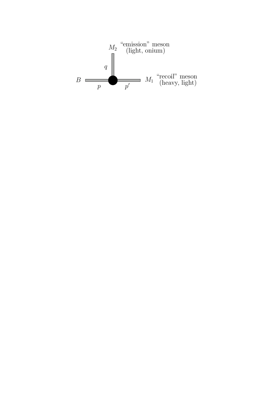
Figure 2: Kinematics and notation.

The simplest diagrams that we can draw for a non-leptonic decay amplitude assign a quark and antiquark to each meson. We choose the quark and antiquark momentum in $M_{2}$ as

$$k_{q}=uq+k_{\perp}+\frac{\vec{k}_{\perp}^{\,2}}{2um_{B}}\,n_{-},\qquad k_{\bar{q}}=\bar{u}q-k_{\perp}+\frac{\vec{k}_{\perp}^{\,2}}{2\bar{u}m_{B}}\,n_{-}.$$ (15)

Note that $q\not=k_{q}+k_{\bar{q}}$, but the off-shellness $(k_{q}+k_{\bar{q}})^{2}$ is of the same order as the light meson mass, which we can neglect at leading power in $1/m_{b}$. A similar decomposition is used for $M_{1}$ in terms of $v$, $p^{\prime}$ and $k_{\perp}^{\prime}$. Let $l$ denote the momentum of the spectator quark. The decay amplitude is then a function

$$A(p^{\prime},q;l;u,k_{\perp};v,k^{\prime}_{\perp})$$ (16)

convoluted with meson wave functions.

We start by considering the case for which $M_{1}$ is heavy. To prove (4) in this case one has to show that:

• There is no leading (in $1/m_{b}$) contribution from the endpoint regions $u\sim\Lambda_{\rm QCD}/m_{b}$ and $\bar{u}\sim\Lambda_{\rm QCD}/m_{b}$.

• One can set $k_{\perp}=0$ in the amplitude (more generally, expand the amplitude in $k_{\perp}$) after collinear subtractions, which can be absorbed into the wave function of $M_{2}$. This, together with 1), guarantees that the amplitude is legitimately expressed in terms of the light-cone distribution amplitude of $M_{2}$.

• The leading contribution comes from $\bar{v}\sim\Lambda_{\rm QCD}/m_{b}$, which guarantees the absence of a hard spectator interaction term.

• After subtraction of infrared contributions corresponding to the light-cone distribution amplitude and the form factor, the leading contributions to the amplitude come only from internal lines with virtuality that scales with $m_{b}$.

• Non-valence Fock states are non-leading.

If $M_{1}$ is light the same statements apply, except that there is now a leading contribution from large momentum transfer to the spectator quark, so that $\bar{v}$ can be of order 1. In order to verify the structure of the third term in the first equation in (4), one then has to show that for any hard spectator interaction the amplitude depends only on $l_{+}$, and that one can set $k^{\prime}_{\perp}=0$ in addition to $k_{\perp}=0$ after collinear subtractions appropriate to the wave functions of $M_{1}$, $M_{2}$ and $B$.

The requirement that after subtractions virtualities should be large is obvious to guarantee the infrared finiteness of the hard-scattering functions $T^{I}_{ij}$ and $T^{II}_{i}$. Let us comment on setting transverse momenta in the wave functions to zero and on endpoint contributions.

Neglecting transverse momenta requires that we count them as order $\Lambda_{\rm QCD}$ when comparing terms of different magnitude in the scattering amplitude. This conforms to our intuition, and the assumption of the parton model, that intrinsic transverse momenta are limited to hadronic scales. However, in QCD transverse momenta are not limited, but logarithmically distributed up to the hard scale. The important point is that those contributions that violate the starting assumption of limited transverse momentum can be absorbed into the universal meson light-cone distribution amplitudes. The statement that transverse momenta can be counted of order $\Lambda_{\rm QCD}$ is to be understood after these subtractions have been performed.

The second comment concerns “endpoint contributions” in the convolution integrals over longitudinal momentum fractions. These contributions are dangerous, because we may be able to demonstrate the infrared safety of the hard-scattering amplitude under assumption of generic $u$ and independent of the shape of the meson distribution amplitude, but for $u\to 0$ or $u\to 1$ a propagator that was assumed to be off-shell approaches the mass-shell. If such a contribution is of leading power, we do not expect the perturbative calculation of the hard-scattering function to be reliable.

Estimating endpoint contributions requires knowledge of the endpoint behaviour of the light-cone distribution amplitude. Since the distribution amplitude enters the factorization formula at a renormalization scale of order $m_{b}$, we can use the asymptotic form of the wave function to estimate the endpoint contribution. (More generally, we only have to assume that the distribution amplitude at a given scale has the same endpoint behaviour as the asymptotic distribution amplitude. This is generally the case, unless there is a conspiracy of terms in the Gegenbauer expansion of the distribution amplitude. If such a conspiracy existed at some scale, it would be immediately destroyed by evolving the distribution amplitude to a slightly different scale.) Using (8) we count a light meson distribution amplitude as order $\Lambda_{\rm QCD}/m_{b}$ in the endpoint region (defined as the region where $u$ or $\bar{u}$ is of order $\Lambda_{\rm QCD}/m_{b}$, such that the quark or antiquark momentum is of order $\Lambda_{\rm QCD}$) and order $1$ away from the endpoint ($X=P,||,\perp$):

$$\Phi_{X}(u)\sim\left\{\begin{array}[]{cl}1\,;&\quad\mbox{generic $u$,}\\[2.84544pt] \Lambda_{\rm QCD}/m_{b}\,;&\quad u,\,\bar{u}\sim\Lambda_{\rm QCD}/m_{b}.\end{array}\right.$$ (17)

Note that the endpoint region has size of order $\Lambda_{\rm QCD}/m_{b}$ so that the endpoint suppression is $\sim(\Lambda_{\rm QCD}/m_{b})^{2}$. This suppression has to be weighted against potential enhancements of the partonic amplitude when one of the propagators approaches the mass shell.

The counting for $B$ mesons, or heavy mesons in general, is different. Given the normalization condition (14), we count

$$\Phi_{B1}(\xi)\sim\left\{\begin{array}[]{cl}m_{b}/\Lambda_{\rm QCD}\,;&\quad\xi\sim\Lambda_{\rm QCD}/m_{b},\\[2.84544pt] 0\,;&\quad\xi\sim 1.\end{array}\right.$$ (18)

The zero probability for a light spectator with momentum of order $m_{b}$ must be understood as a boundary condition for the wave function renormalized at a scale much below $m_{b}$. There is a small probability for hard fluctuations that transfer large momentum to the spectator as discussed above. This “hard tail” is generated by evolution of the wave function from a hadronic scale to a scale of order $m_{b}$. If we assume that the initial distribution at the hadronic scale falls sufficiently rapidly for $\xi\gg\Lambda_{\rm QCD}/m_{b}$, this remains true after evolution. We shall assume a sufficiently fast fall-off, so that, for the purposes of power counting, the probability that the $l_{+}$ ($=\xi p_{+}$) component of the spectator quark’s momentum is of order $m_{b}$ can be set to zero. If $M_{1}$ is a heavy meson, the same counting that applies to the $B$ meson is valid also for $M_{1}$. Despite the fact that $M_{1}$ has momentum of order $m_{b}$, we do not need to distinguish the $B$- and $M_{1}$-meson rest frames for the purpose of power counting, because the two frames are not connected by a parametrically large boost (i.e. the Lorentz factor of the boost is of order 1 and not of order $m_{b}/\Lambda_{\rm QCD}$). In other words, the components of the spectator quark in $M_{1}$ are still of order $\Lambda_{\rm QCD}$.

3.2 The $B\to M_{1}$ form factor

We now consider the form factor for the $B\to M_{1}$ transition and demonstrate that it receives a leading contribution from soft gluon exchange. This implies that a non-leptonic decay cannot be treated completely in the hard-scattering picture, and therefore that the form factor should enter the factorization formula as a non-perturbative quantity, as in (4). We begin the argument with the diagrams shown in Fig. 3, which would be leading if the $B\to M_{1}$ transition could be considered as a hard process. We shall also establish how the form factors scale with the mass of the heavy quark.

Figure 3: Leading contributions to the $B\to M_{1}$ form factor in the hard-scattering approach. The dashed line represents the weak current. The two lines to the left belong to the $B$ meson, the ones to the right to the recoil meson $M_{1}$.

3.2.1 $M_{1}$ heavy ($B\to D$ transitions)

The case when the final-state meson is heavy, for example a $D$ meson, is particularly simple. When the gluon exchanged in Fig. 3 is hard, the final spectator quark has momentum of order $m_{b}$. According to the counting rule (18) this configuration has no overlap with the $D$-meson wave function. On the other hand, there is no suppression for soft gluons in Fig. 3. It follows that the dominant behaviour of the $B\to D$ form factor in the heavy-quark limit is given by soft processes.

To answer the question how the form factor scales in the heavy-quark limit, we note that since the form factor is dominated by soft processes we can exploit the heavy-quark symmetries. (The discussion in this section aims only at counting powers of $m_{b}$, that is we ignore logarithmic effects in $m_{b}$ which arise from hard corrections to the $b\to c$ vertex.) Heavy-quark symmetry implies that the form factor scales like a constant, since it is equal to one at zero velocity transfer and is independent of $m_{b}$ as long as the Lorentz boost that connects the $B$ and $D$ rest frames is independent of $m_{b}$. The same conclusion also follows from the power-counting rules for light-cone wave functions. To see this, we represent the form factor by an overlap integral of light-cone wave functions (not integrated over transverse momentum),

$$F_{+,0}^{B\to D}(0)\sim\int\frac{d\xi d^{2}k_{\perp}}{16\pi^{3}}\,\Psi_{B}(\xi,k_{\perp})\,\Psi_{D}(\xi^{\prime}(\xi),k_{\perp}),$$ (19)

where $\xi^{\prime}(\xi)$ is fixed by kinematics and we have set $q^{2}=0$. The probability of finding the $B$ meson in its valence Fock state is of order 1 in the heavy-quark limit, i.e.

$$\int\frac{d\xi d^{2}k_{\perp}}{16\pi^{3}}\,|\Psi_{B,D}(\xi,k_{\perp})|^{2}\sim 1.$$ (20)

Counting $k_{\perp}\sim\Lambda_{\rm QCD}$ and $d\xi\sim\Lambda_{\rm QCD}/m_{b}$, we deduce that $\Psi_{B}(\xi,k_{\perp})\sim m_{b}^{1/2}/\Lambda_{\rm QCD}^{3/2}$. An alternative way to arrive at this result uses the relation

$$\Phi_{B}(\xi)\sim\frac{1}{f_{B}}\,\,\int_{k_{\perp}<\mu}\!\!d^{2}k_{\perp}\Psi_{B}(\xi,k_{\perp}),$$ (21)

together with $f_{B}\sim\Lambda_{\rm QCD}^{3/2}/m_{b}^{1/2}$ and the normalization condition for $\Phi_{B}(\xi)$. From (19), we then obtain the scaling law

$$F_{+,0}^{B\to D}(0)\sim 1,$$ (22)

in agreement with our earlier power-counting estimate. The representation (19) of the form factor as an overlap of wave functions for the two-particle Fock components of the heavy-meson wave function is not rigorous, because there is no reason to assume that the contribution from higher Fock states with additional soft gluons is suppressed. The consistency with the estimate based on heavy-quark symmetry shows that these additional contributions are not larger than the two-particle contribution.

3.2.2 $M_{1}$ light ($B\to\pi$ transitions)

The case of the heavy-light form factor is more complicated. When the exchanged gluon in Fig. 3 is soft, one of the quark constituents of $M_{1}$ is soft (for the purpose of illustration, for the remainder of this subsection we will take $M_{1}$ to be a pion). This configuration is suppressed by the endpoint behaviour of the pion distribution amplitude given by (17). In addition we now also have a hard contribution, for which there is no wave-function suppression.

We begin with the hard contribution. By assumption both quarks that form the pion have longitudinal momenta of order $m_{b}$, so that the virtuality of the exchanged gluon is of order $m_{b}\Lambda_{\rm QCD}$. These gluons can be treated perturbatively in the heavy-quark limit. The calculation of the diagrams shown in Fig. 3, setting $q^{2}=0$ as an example, results in

$$F_{+,0}^{B\to\pi}(0) = \frac{\pi\alpha_{s}C_{F}}{N_{c}}\,\frac{f_{\pi}f_{B}}{m_{b}^{2}}\int_{0}^{1}d\xi du\,[\Phi_{B1}(\xi)-2\Phi_{B2}(\xi)]\,\Phi_{\pi}(u)\,\frac{1}{\xi\bar{u}^{2}}$$ (23)

$$\,+\,\mbox{terms with }1/\bar{u}.$$

(For the calculation of the $1/\bar{u}$ term the $B$-meson distribution amplitude has to be generalized as indicated after (13). However, the precise expression for the $1/\bar{u}$ term is not necessary for the subsequent discussion.) With $\bar{u}\sim 1$, $\xi\sim\Lambda_{\rm QCD}/m_{b}$ and the scaling behaviours of the distribution amplitudes discussed earlier, we obtain

$$F_{+,0;\,\rm hard}^{B\to\pi}(0)\sim\alpha_{s}(\sqrt{m_{b}\Lambda_{\rm QCD}})\,\left(\frac{\Lambda_{\rm QCD}}{m_{b}}\right)^{\!3/2}.$$ (24)

To our knowledge, this scaling behaviour was first derived in [16].

However, the computation of the hard contribution is not self-consistent. With $\Phi_{\pi}(u)\propto u\bar{u}$, the integral in (23) diverges logarithmically for $u\to 1$ [17, 18]. In this limit the momentum of the exchanged gluon approaches zero. If we interpret $\alpha_{s}$ times this logarithmic divergence as a constant of order 1, we obtain an estimate for the soft contribution to the form factor:

$$F_{+,0;\,\rm soft}^{B\to\pi}(0)\sim\left(\frac{\Lambda_{\rm QCD}}{m_{b}}\right)^{\!3/2}.$$ (25)

There is an alternative way to arrive at this result. As in (19) we represent the soft contribution to the form factor by an overlap integral of wave functions not integrated over transverse momentum. The difference is that for $u(\xi)\sim\Lambda_{\rm QCD}/m_{b}$ the wave function for the pion scales as $\Psi_{\pi}(u(\xi),k_{\perp})\sim 1/m_{b}$. Eq. (25) then follows from (19). We therefore conclude that the hard and soft contributions to the heavy-light form factor have the same scaling behaviour in the heavy-quark limit. The hard contribution is suppressed by one power of $\alpha_{s}$. This is why the standard approach to hard, exclusive processes [7, 8] is not applicable to heavy-light form factors, as noticed already in [16]. Note that both ways of arriving at this conclusion make use of the fact that the pion’s light-cone distribution amplitude vanishes linearly near the endpoints $u=0$ or 1. Since the applicability of the Fock-state expansion is doubtful for endpoint regions, relying on the endpoint behaviour of the two-particle wave function makes the power-counting estimate (25) appear less solid than the estimate for the $B\to D$ form factor.

The dominance of the soft contribution has been a major motivation for applying light-cone QCD sum rules to the calculation of the $B\to\pi$ form factor [16]. In this framework, the leading contribution is again given by a diagram that corresponds to the soft overlap term. The first order radiative correction [9, 10] contains both hard and soft contributions, in accordance with the above discussion. Furthermore, the heavy-quark scaling is also consistent with the one observed above [10]. However, it should be noted that the heavy-quark scaling law in the framework of QCD sum rules also relies on the endpoint behaviour of the pion wave function and therefore does not provide an independent verification of the scaling behaviour.

The upshot of this discussion is that the heavy-to-light form factor is not fully calculable in perturbative QCD (using light-cone distribution amplitudes), because the form factor is dominated by a soft endpoint contribution. At this point, it is worth recalling that we have neglected logarithmic effects in $m_{b}$. Summing such logarithms results in a Sudakov form factor that suppresses the kinematic configuration when almost all momentum in the $b\to u$ transition is transferred to the $u$ quark, i.e. it suppresses the singularity at $u=1$ in (23). (A similar situation occurs for the pion form factor at next-to-leading power and is discussed in [19].) If the soft contribution were suppressed sufficiently by the Sudakov form factor, as would be the case in the limit of an asymptotically large bottom quark mass, the heavy-to-light form factor would be calculable perturbatively in terms of light-cone distribution amplitudes. By the arguments provided later in this section, the entire non-leptonic decay amplitude into two light mesons (but not a heavy and a light meson) could then be brought into the form of the second line of the first equation in (4). This observation is the starting point for the hard-scattering approach to non-leptonic decays as discussed further in Sect. 7. However, it appears unlikely to us that Sudakov suppression makes the soft contribution negligible for $m_{b}\approx 5\,$GeV. For this reason we prefer to keep the factorization formula in the more general form of (4). The important point is that factorization is still valid under less restrictive assumptions that admit a soft contribution to the heavy-light form factor. Nothing is lost keeping this more general form, as the form factor, which then appears as an additional non-perturbative input, can be obtained experimentally or from other methods.

We shall see later that the first and second line in the factorization formula (4) are of the same order in the heavy-quark limit, but that the second line is suppressed by one power of $\alpha_{s}$. This conclusion depends on the assumed endpoint behaviour of the light-cone distribution amplitude of a light meson and on neglecting a potential Sudakov suppression of the endpoint contribution. Let us mention what changes if these assumptions are not valid. If Sudakov suppression is effective, or if the light-cone distribution amplitude vanishes more rapidly than linearly near the endpoint, then the hard contribution to the form factor is leading and both terms in the factorization formula are of the same order in the heavy-quark limit and in $\alpha_{s}$. If, on the other hand, the light meson distribution amplitude vanishes less rapidly than linearly near the endpoint, or if soft effects are larger than indicated by the endpoint behaviour of the two-particle wave function, then the first line in (4) becomes more important. (If the wave function does not vanish at the endpoint, the factorization formula breaks down.) In the following we shall assume the canonical endpoint behaviour provided by the asymptotic wave function. We shall also restrict ourselves to power counting and neglect possible Sudakov form factors.

To conclude this discussion of the form factor, we also mention that a complete treatment of logarithms of $m_{b}$ goes far beyond the Sudakov form factor mentioned above. The factor $1/\bar{u}^{2}$ that causes the divergence of the integral in (23) comes only from the first diagram of Fig. 3. In [20] this term is absorbed into a redefinition of the $B$-meson wave function by an eikonal phase. If this could be done to all orders, this would remove the need to include a soft contribution to the form factor at leading power in $1/m_{b}$, at least in perturbation theory. It is then shown in [20] that there is another Sudakov form factor that suppresses the contribution from the small-$\xi$ region to the integral in (23). A complete discussion of logarithms of $m_{b}$ to all orders in perturbation theory has, to our knowledge, never been given. We shall not pursue this in this paper, too, since we use the form factor as an input.

3.3 Non-leptonic decay amplitudes

We now turn to the qualitative discussion of the lowest-order and one-gluon exchange diagrams that could contribute to the hard-scattering kernels $T^{I}_{ij}(u)$ and $T^{II}_{i}(\xi,u,v)$ in (4). In the figures which follow, with the exception of the annihilation diagrams, the two lines directed upwards represent $M_{2}$, which we shall assume to be a $\pi^{-}$ for definiteness. The two lines on the left represent the $\bar{B}_{d}$, the lower line being the light $\bar{d}$ spectator. The two lines directed to the right represent $M_{1}$, taken to be a $D^{+}$ or $\pi^{+}$ for definiteness. The black square marks the weak decay vertex for $b\to q\bar{u}d$ where $q=c,u$ (see also Fig. 2).

3.3.1 Lowest-order diagram

Figure 4: Leading-order contribution to the hard-scattering kernel $T^{I}_{ij}(u)$. The weak decay of the $b$ quark through a four-fermion operator (of current-current or penguin type) is represented by the black square. See text and Fig. 2 for further notation.

There is a single diagram with no hard gluon interactions shown in Fig. 4. According to (18) the spectator quark is soft, and since it does not undergo a hard interaction it is absorbed as a soft quark by the recoiling meson. This is evidently a contribution to the left-hand diagram of Fig. 1, involving the $B\to D$ ($B\to\pi$) form factor in the case of $\bar{B}_{d}\to D^{+}\pi^{-}$ ($\bar{B}_{d}\to\pi^{+}\pi^{-}$). The hard subprocess in Fig. 4 is just given by the insertion of a four-fermion operator and hence it does not depend on the longitudinal momentum fraction $u$ of the two quarks that form the emitted $\pi^{-}$. Consequently, the lowest-order contribution to $T_{ij}^{I}(u)$ in (4) is independent of $u$, and the $u$-integral reduces to the normalization condition for the pion wave function. The result is, not surprisingly, that the factorization formula (4) reproduces the result of naive factorization, if we neglect gluon exchange.

Note that the physical picture underlying this lowest-order process is that the spectator quark (which is part of the $B\to D$ or $B\to\pi$ form factor) is soft. If this is the case, the hard-scattering approach misses the leading contribution to the non-leptonic decay amplitude.

Putting together all factors relevant to power counting we find that, in the heavy-quark limit, the decay amplitude scales as

$${\cal A}(\bar{B}_{d}\to D^{+}\pi^{-})\sim G_{F}m_{b}^{2}\,F^{B\to D}(0)\,f_{\pi}\sim G_{F}m_{b}^{2}\,\Lambda_{\rm QCD}$$ (26)

for a decay into a heavy-light final state (in which the spectator quark is absorbed by the heavy meson), and

$${\cal A}(\bar{B}_{d}\to\pi^{+}\pi^{-})\sim G_{F}m_{b}^{2}\,F^{B\to\pi}(0)\,f_{\pi}\sim G_{F}m_{b}^{1/2}\,\Lambda^{5/2}_{\rm QCD}$$ (27)

for a decay into two light mesons. Other contributions must be compared with these scaling rules.

3.3.2 Factorizable diagrams

Figure 5: Diagrams at order $\alpha_{s}$ that need not be calculated.

In order to justify naive factorization (Fig. 4) as the leading term in an expansion in $\alpha_{s}$ and $\Lambda_{\rm QCD}/m_{b}$, we must show that radiative corrections are either suppressed in one of these two parameters, or already contained in the definition of the form factor and the decay constant of $M_{2}$ (the pion).

Consider the diagrams shown in Fig. 5. The first three diagrams are part of the form factor and do not contribute to the hard-scattering kernels. Since the first and third diagrams contain leading contributions from the region in which the gluon is soft (as discussed for the first diagram in the previous subsection), they should not be considered as corrections to Fig. 4. This is of no consequence since these soft contributions are absorbed into the physical form factor. The diagrams also have hard contributions, which we could isolate and compute. For instance, the hard contributions in the third diagram are those that go into the short-distance coefficient when the physical form factor is matched onto the heavy-to-heavy or heavy-to-light form factor in heavy-quark effective theory. However, we do not perform this matching here, neither do we attempt to construct a factorization formula for the heavy-light form factor itself. Rather, the form factor that appears in (4) is the form factor in full QCD, which is also the one directly measured in experiments.

The fourth diagram in Fig. 5 is also factorizable. In general, this diagram would split into a hard contribution and a contribution to the evolution of the pion distribution amplitude. However, as the leading-order diagram (Fig. 4) involves only the normalization integral of the pion distribution amplitude, the sum of the fourth diagram in Fig. 5 and the wave-function renormalization of the quarks in the emitted pion vanishes. In other words, these diagrams renormalize the $(\bar{u}d)$ light-quark $V-A$ current, which however is conserved.

3.3.3 “Non-factorizable” vertex corrections

Figure 6: “Non-factorizable” vertex corrections.

We now begin the analysis of “non-factorizable” diagrams, i.e. diagrams containing gluon exchanges that do not belong to the form factor for the $B\to M_{1}$ transition or the decay constant of $M_{2}$. At order $\alpha_{s}$ these diagrams can be divided into four groups: vertex corrections, penguin diagrams, hard spectator interactions and annihilation diagrams. We discuss these four cases in turn.

The vertex corrections shown in Fig. 6 violate the naive factorization ansatz (2). One of the key points of this paper is that these diagrams are calculable nonetheless. Let us summarize the argument here. The explicit evaluation of these diagrams can be found in Sect. 4. A generalization of the argument to higher orders is given in Sect. 5.

The statement is that these diagrams form an order-$\alpha_{s}$ correction to the hard-scattering kernel $T^{I}_{ij}(u)$. To demonstrate this, we have to show that: (a) The transverse momentum of the quarks that form $M_{2}$ can be neglected at leading power, i.e. the two momenta in (15) can be approximated by $uq$ and $\bar{u}q$, respectively. This guarantees that only a convolution in the longitudinal momentum fraction $u$ appears in the factorization formula. (b) The contribution from the soft-gluon region and gluons collinear to the direction of $M_{2}$ and $M_{1}$ (if $M_{1}$ is light) is power suppressed. In practice this means that the sum of these diagrams cannot contain any infrared divergences at leading power in $1/m_{b}$.

Neither of the two conditions holds true for any of the four diagrams individually, as each of them separately is collinearly and infrared divergent. As will be shown in detail later, the infrared divergences cancel when one sums over the gluon attachments to the two quarks comprising the emission pion ((a+b), (c+d) in Fig. 6). This cancellation is a technical manifestation of Bjorken’s colour-transparency argument [11]: soft gluon interactions with the emitted colour-singlet $\bar{u}d$ pair are suppressed, because they interact only with the colour dipole moment of the compact light-quark pair. Collinear divergences cancel after summing over gluon attachments to the $b$ and $c$ (or $u$) quark line ((a+c), (b+d) in Fig. 6); in the light-cone gauge, collinear divergences are absent altogether. Thus the sum of the four diagrams (a-d) involves only hard gluon exchange at leading power. Because the hard gluons transfer large momentum to the quarks that form the emission pion, the hard-scattering factor now results in a non-trivial convolution with the pion distribution amplitude. “Non-factorizable” contributions are therefore non-universal, i.e. they depend on what type of meson $M_{2}$ is.

Note that the colour-transparency argument, and hence the cancellation of soft gluon effects, applies only if the $\bar{u}d$ pair is compact. This is not the case if the emitted pion is formed in a very asymmetric configuration, in which one of the quarks carries almost all of the pion’s momentum. Since the probability for forming a pion in such an endpoint configuration is of order $(\Lambda_{\rm QCD}/m_{b})^{2}$, they could become important only if the hard-scattering amplitude favoured the production of these asymmetric pairs, i.e. if $T^{I}_{ij}\sim 1/u^{2}$ for $u\to 0$ (or $T^{I}_{ij}\sim 1/\bar{u}^{2}$ for $u\to 1$). However, such strong endpoint singularities in the hard-scattering amplitude do not occur.

3.3.4 Penguin diagrams

Figure 7: Diagram with a “penguin” contraction. The second diagram represents a contribution from the chromomagnetic dipole operator in the weak effective Hamiltonian.

The penguin diagram (first diagram in Fig. 7) exists for $\bar{B}_{d}\to\pi^{+}\pi^{-}$ but not for $\bar{B}_{d}\to D^{+}\pi^{-}$. We need to show again that, at leading order in $1/m_{b}$, all internal lines in this diagram are hard.

Consider first the two final-state quarks into which the gluon splits. The quark that goes into the recoil $\pi^{+}$ to the right must always be energetic to make an energetic pion, because the $\bar{d}$ spectator quark is soft. The configuration in which the other quark is soft is suppressed by the endpoint behaviour of the light-cone distribution amplitude of the $\pi^{-}$. We conclude that the gluon splits into two energetic quarks that fly in opposite directions, and that the gluon has large virtuality $\sim\bar{u}m_{b}^{2}$, where $\bar{u}$ is the longitudinal momentum fraction of the antiquark in the $\pi^{-}$. In principle, one of the quarks in the quark loop can still be soft, if the loop momentum is soft and the gluon momentum flows asymmetrically through the loop. But this configuration is suppressed by two powers of $\Lambda_{\rm QCD}/m_{b}$ relative to the configuration where both quarks carry large momentum of order $m_{b}$, as follows from the structure of a vacuum polarization diagram. As a result the penguin diagram contributes to the hard-scattering kernel $T_{ij}^{I}(u)$ at order $\alpha_{s}$, just as the vertex diagrams do. The same argument shows that the chromomagnetic dipole diagram (second diagram in Fig. 7) is also a calculable correction to the hard-scattering kernel. An explicit calculation of these diagrams can be found in [1].

Note that this argument provides a rigorous justification for the Bander-Silverman-Soni (BSS) mechanism [21] to generate strong-interaction phases perturbatively by means of the rescattering phase of the penguin loop. In particular, the gluon virtuality $k^{2}=\bar{u}m_{b}^{2}$, which is usually treated as a phenomenological parameter, is unambiguously determined by the kinematics of the decay process together with the weighting of $\bar{u}$ implied by the pion wave function. At the same time it should be noted that the BSS mechanism does not provide a complete description of final-state interactions even in the heavy-quark limit, as the vertex diagrams (c,d) of Fig. 6 also generate imaginary parts, which are of the same order as those of the penguin diagram. A more detailed discussion of final-state interaction phases will be presented in Sect. 3.4.

3.3.5 Hard spectator interaction

Figure 8: “Non-factorizable” spectator interactions.

Up to this point, we have not obtained a contribution to the second line of (4), i.e. to the hard-scattering term in Fig. 1 (as opposed to the form-factor term). The diagrams shown in Fig. 8 cannot be associated with the form-factor term. These diagrams would impede factorization if there existed a soft contribution at leading power. While such terms are present in each of the two diagrams separately, to leading power they cancel in the sum over the two gluon attachments to the $\bar{u}d$ pair by the same colour-transparency argument that was applied to the “non-factorizable” vertex corrections. For decays into two light mesons there is a further suppression of soft gluon exchange because of the endpoint suppression of the light-cone distribution amplitude for the recoiling meson $M_{1}$.

We consider first the decay into a heavy and a light meson ($\bar{B}_{d}\to D^{+}\pi^{-}$) in more detail. We still have to show that after the soft cancellation the remaining soft contribution is power suppressed relative to the leading-order contribution (26). A straightforward calculation leads to the following (simplified) result for the sum of the two diagrams:

$${\cal A}(\bar{B}_{d}\to D^{+}\pi^{-})_{({\rm Fig.~{}\ref{fig8}})} \sim G_{F}\,f_{\pi}f_{D}f_{B}\,\alpha_{s}\,\int_{0}^{1}\frac{d\xi}{\xi}\,\Phi_{B1}(\xi)\int_{0}^{1}\frac{d\eta}{\eta}\,\Phi_{D1}(\eta)\int_{0}^{1}\frac{du}{u}\,\Phi_{\pi}(u)$$ (28)

$$\sim G_{F}\,\alpha_{s}\,m_{b}\,\Lambda_{\rm QCD}^{2}.$$

This is indeed power suppressed relative to (26). Note that the gluon virtuality is of order $\xi\eta m_{b}^{2}\sim\Lambda_{\rm QCD}^{2}$ and so, strictly speaking, the calculation in terms of light-cone distribution amplitudes cannot be justified. Nevertheless, we use (28) to estimate the size of the soft contribution, as we did for the heavy-light form factor. On the contrary, when the gluon is hard, it transfers large momentum to the spectator quark. According to our power-counting rule (18), such a configuration has no overlap with either the $B$- or the $D$-meson wave function. We therefore conclude that the hard spectator interaction does not contribute to heavy-light final states at leading power in the heavy-quark expansion. The factorization formula (4) then assumes a simpler form, with the second line omitted, as discussed earlier.

For decays into two light mesons ($\bar{B}_{d}\to\pi^{+}\pi^{-}$) the explicit expression for the sum of the two diagrams is similar to the one above [1]:

$${\cal A}(\bar{B}_{d}\to\pi^{+}\pi^{-})_{({\rm Fig.~{}\ref{fig8}})} \sim G_{F}\,f_{\pi}^{2}f_{B}\,\alpha_{s}\,\int_{0}^{1}\frac{d\xi}{\xi}\,\Phi_{B1}(\xi)\int_{0}^{1}\frac{dv}{\bar{v}}\,\Phi_{\pi}(v)\int_{0}^{1}\frac{du}{u}\,\Phi_{\pi}(u)$$ (31)

$$\sim\left\{\begin{array}[]{ll}G_{F}\,\alpha_{s}\,m_{b}^{1/2}\,\Lambda_{\rm QCD}^{5/2}\,;&\mbox{hard gluon},\\[2.84544pt] G_{F}\,\alpha_{s}\,m_{b}^{-1/2}\,\Lambda_{\rm QCD}^{7/2}\,;&\mbox{soft gluon}.\end{array}\right.$$

The soft contribution is suppressed as discussed above, but the hard contribution is of the same order as (27), with an additional factor of $\alpha_{s}$. (The hard gluon has momentum of order $m_{b}$, but its virtuality is only of order $m_{b}\Lambda_{\rm QCD}$, similar to the hard contribution to the $B\to\pi$ form factor.) Eq. (31) results in a contribution to the second hard-scattering kernel, $T^{II}_{i}(\xi,u,v)$, in (4). In the heavy-quark limit, the hard spectator interaction is of the same order as the vertex corrections and penguin contributions to the first hard-scattering kernel. (See, however, the comments at the end of Sect. 3.2 concerning a modification of this statement in the presence of Sudakov form factors.)

3.3.6 Annihilation topologies

Figure 9: Annihilation diagrams.

Our final concern in this subsection are the annihilation diagrams (Fig. 9) which contribute to $\bar{B}_{d}\to D^{+}\pi^{-}$ and $\bar{B}_{d}\to\pi^{+}\pi^{-}$. The hard part of these diagrams would amount to another contribution to the second hard-scattering kernel, $T^{II}_{i}(\xi,u,v)$. The soft part, if unsuppressed, would violate factorization. However, we shall show now that the hard part as well as the soft part are suppressed by at least one power of $\Lambda_{\rm QCD}/m_{b}$.

Light-light final states ($\bar{B}_{d}\to\pi^{+}\pi^{-}$)

We begin with the two diagrams (a,b). Suppose first that all four light quarks in the final state are energetic. Then the virtuality of the gluon is of order $m_{b}^{2}$. If we now let one of the quarks be soft, the gluon virtuality can decrease to $m_{b}\Lambda_{\rm QCD}$ and the amplitude is then enhanced by a factor $m_{b}/\Lambda_{\rm QCD}$. (In particular cases, the virtuality of the internal quark line can also become small. However, closer inspection shows that in this case the numerator also becomes small and there is no further enhancement of the amplitude.) This enhancement is over-compensated by a suppression with two powers of $\Lambda_{\rm QCD}/m_{b}$, where one power arises from the endpoint behaviour of the pion distribution amplitude and another from the small region of phase space considered. The configuration where two final-state quarks are soft is even further suppressed. It follows that the leading contribution to (a,b) arises when all four quarks are energetic. Since the integral over the $B$-meson wave function simply gives the normalization integral, it is easy to see that the diagrams scale at most as

$$G_{F}\,f_{\pi}^{2}f_{B}\alpha_{s}\sim G_{F}\,\alpha_{s}m_{b}^{-1/2}\Lambda_{\rm QCD}^{7/2},$$ (32)

which is one power of $\Lambda_{\rm QCD}/m_{b}$ smaller than (27). (In fact, current conservation implies that the result is proportional to the difference of quark masses at the annihilation vertex. Hence the sum of (a) and (b) vanishes for $\bar{B}_{d}\to\pi^{+}\pi^{-}$.)

The hard part of diagrams (c,d) (all four quarks energetic) obviously also scales as (32). A difference to (a,b) arises when some of the quarks are soft. For emission of the light $q\bar{q}$ pair from the $B$-meson spectator quark (diagram (d)) it may happen that the endpoint contribution from a single soft final-state quark is not suppressed relative to the hard part, because the amplitude is enhanced by a large internal gluon and quark propagator. (But since the gluon virtuality is still of order $m_{b}\Lambda_{\rm QCD}$, there remains a factor $\alpha_{s}(\sqrt{m_{b}\Lambda_{\rm QCD}})$). However, since the hard part is power suppressed relative to (27), power suppression continues to hold for the entire graph.

Heavy-light final states ($\bar{B}_{d}\to D^{+}\pi^{-}$)

The power counting is different for $\bar{B}_{d}\to D^{+}\pi^{-}$, because the light quark that goes into the $D$ meson must always be soft according to (18), and hence the virtuality of the gluon is never larger than $m_{b}\Lambda_{\rm QCD}$. Nevertheless, we obtain power suppression also in this case. The argument is as follows. We can write the annihilation amplitude as

$${\cal A}(\bar{B}_{d}\to D^{+}\pi^{-})_{({\rm Fig.~{}\ref{fig9}})}\sim G_{F}\,f_{\pi}f_{D}f_{B}\,\alpha_{s}\,\int_{0}^{1}d\xi d\eta du\,\Phi_{B1}(\xi)\,\Phi_{D1}(\eta)\,\Phi_{\pi}(u)\,T^{\rm ann.}(\xi,\eta,u),$$ (33)

where the dimensionless function $T^{\rm ann.}(\xi,\eta,u)$ is a product of propagators and vertices. The product of decay constants scales as $\Lambda_{\rm QCD}^{4}/m_{b}$. Since $d\xi\,\Phi_{B1}(\xi)$ scales as 1 and so does $d\eta\,\Phi_{D1}(\eta)$, while $du\,\Phi_{\pi}(u)$ is never larger than 1, the amplitude can only compete with the leading-order result (26) if $T^{\rm ann.}(\xi,\eta,u)$ can be made of order $(m_{b}/\Lambda_{\rm QCD})^{3}$ or larger. Since $T^{\rm ann.}(\xi,\eta,u)$ contains only two propagators, this can be achieved only if both quarks the gluon splits into are soft, in which case $T^{\rm ann.}(\xi,\eta,u)\sim(m_{b}/\Lambda_{\rm QCD})^{4}$. But then $du\,\Phi_{\pi}(u)\sim(\Lambda_{\rm QCD}/m_{b})^{2}$ so that this contribution is power suppressed.

3.3.7 Summary

To summarize the discussion up to this point: for the decay into a light emitted and a heavy recoiling meson (such as our example $\bar{B}_{d}\to D^{+}\pi^{-}$) the second factorization formula in (4) holds. The hard-scattering kernel $T^{I}_{ij}(u)$ is computed in lowest order from the diagram shown in Fig. 4, and at order $\alpha_{s}$ from the vertex diagrams in Fig. 6. For decays into two light mesons, the more complicated first formula in (4) applies. Then, in addition to the vertex diagrams, there are penguin contributions (Fig. 7) to the kernel $T^{I}_{ij}(u)$, and there is a non-vanishing hard-scattering term in (4). The kernel $T_{i}^{II}(\xi,u,v)$ is computed from the diagrams shown in Fig. 8. In both cases, naive factorization follows when one neglects all corrections of order $\Lambda_{\rm QCD}/m_{b}$ and of order $\alpha_{s}$. Eq. (4) allows us to compute systematically corrections to higher order in $\alpha_{s}$, but still neglects power corrections of order $\Lambda_{\rm QCD}/m_{b}$.

Some of the loop diagrams entering the calculation of the hard-scattering kernels have imaginary parts which contribute to the strong rescattering phases. It follows from our discussion that these imaginary parts are of order $\alpha_{s}$ or $\Lambda_{\rm QCD}/m_{b}$. This demonstrates that strong phases vanish in the heavy-quark limit (unless the real parts of the amplitudes are also suppressed). Since this statement goes against the folklore that prevails from the present understanding of this issue, we shall return to this point in Sect. 3.4.

In a common terminology, the decays which we have treated explicitly so far are called “class-I” decays. The distinction of “class-I”, “class-II” and “class-III” decays refers to colour factors and charge combinatorics arising in naive factorization. It is clear that this distinction is not relevant to QCD factorization in the sense of (4), which relies on the hardness and virtuality of partons. This means that the factorization formula applies to any decay into two light mesons, irrespective of whether the decay is class-I, class-II or dominated by penguin operators. Factorization also works for all decays into heavy-light final states, in which the light spectator quark in the $B$ meson is absorbed by the heavy final-state particle (class-I). Factorization does not work for a heavy-light final state, when the spectator quark is picked up by the light meson (class-II), for example $\bar{B}_{d}\to\pi^{0}D^{0}$. We will return to this point in Sect. 3.5.

Our discussion has so far been based on the leading two-particle valence-quark Fock state of the mesons. To complete the discussion we shall argue in Sect. 3.6 that the contributions to the decay amplitude from higher Fock components of the meson wave functions are power suppressed. In Sect. 3.7 we will discuss some of the limitations of the applicability of the factorization formula in practice, recalling that the physical mass of the $b$ quark is not asymptotically large.

3.4 Remarks on final-state interactions

Since the subject of final-state interactions, and of strong-interaction phases in particular, is of paramount importance for the interpretation of CP-violating observables, we discuss here in some more detail the implications of QCD factorization for this issue.

Final-state interactions are usually discussed in terms of intermediate hadronic states. This is suggested by the unitarity relation (taking $B\to\pi\pi$ for definiteness)

$$\mbox{Im}\,{\cal A}_{B\to\pi\pi}\sim\sum_{n}{\cal A}_{B\to n}{\cal A}_{n\to\pi\pi}^{*},$$ (34)

where $n$ runs over all hadronic intermediate states. We can also interpret the sum in (34) as extending over intermediate states of partons. The partonic interpretation is justified by the dominance of hard rescattering in the heavy-quark limit. In this limit the number of physical intermediate states is arbitrarily large. We may then argue on the grounds of parton-hadron duality that their average is described well enough (up to $\Lambda_{\rm QCD}/m_{b}$ corrections, say) by a partonic calculation. This is the picture implied by (4). The hadronic language is in principle exact. However, the large number of intermediate states makes it intractable to observe systematic cancellations, which usually occur in an inclusive sum over hadronic intermediate states.

A particular contribution to the right-hand side of (34) is elastic rescattering ($n=\pi\pi$). The energy dependence of the total elastic $\pi\pi$-scattering cross section is governed by soft pomeron behaviour. Hence the strong-interaction phase of the $B\to\pi\pi$ amplitude due to elastic rescattering alone increases slowly in the heavy-quark limit [22]. On general grounds, it is rather improbable that elastic rescattering gives an appropriate representation of the imaginary part of the decay amplitude in the heavy-quark limit. This expectation is also borne out in the framework of Regge behaviour, as discussed in [22], where the importance (in fact, dominance) of inelastic rescattering is emphasized. However, the approach pursued in [22] leaves open the possibility of soft rescattering phases that do not vanish in the heavy-quark limit, as well as the possibility of systematic cancellations, for which the Regge approach does not provide an appropriate theoretical framework.

Eq. (4) implies that such systematic cancellations do occur in the sum over all intermediate states $n$. It is worth recalling that similar cancellations are not uncommon for hard processes. Consider the example of $e^{+}e^{-}\to\,$hadrons at large energy $q$. While the production of any hadronic final state occurs on a time scale of order $1/\Lambda_{\rm QCD}$ (and would lead to infrared divergences if we attempted to describe it using perturbation theory), the inclusive cross section given by the sum over all hadronic final states is described very well by a $q\bar{q}$ pair that lives over a short time scale of order $1/q$. In close analogy, while each particular hadronic intermediate state $n$ in (34) cannot be described partonically, the sum over all intermediate states is accurately represented by a $q\bar{q}$ fluctuation of small transverse size of order $1/m_{b}$. Because the $q\bar{q}$ pair is small, the physical picture of rescattering is very different from elastic $\pi\pi$ scattering.

In perturbation theory, the pomeron is associated with two-gluon exchange. The analysis of two-loop contributions to the non-leptonic decay amplitude in Sect. 5 shows that the soft and collinear cancellations that guarantee the partonic interpretation of rescattering extend to two-gluon exchange. (Strictly speaking, the analysis of Sect. 5 applies only to decays into a heavy and a light meson. However, the cancellation in the soft-soft region, which is relevant to the present discussion, goes through unmodified if both final-state mesons are light.) Hence, the soft final-state interactions are again subleading as required by the validity of (4). As far as the hard rescattering contributions are concerned, two-gluon exchange plus ladder graphs between a compact $q\bar{q}$ pair with energy of order $m_{b}$ and transverse size of order $1/m_{b}$ and the other pion does not lead to large logarithms, and hence there is no possibility to construct the (hard) pomeron. Note the difference with elastic vector-meson production through a virtual photon, which also involves a compact $q\bar{q}$ pair. However, in this case one considers $s\gg Q^{2}$, where $\sqrt{s}$ is the photon-proton center-of-mass energy and $Q$ the virtuality of the photon. This implies that the $q\bar{q}$ fluctuation is born long before it hits the proton. It is this difference of time scales, non-existent in non-leptonic $B$ decays, that permits pomeron exchange in elastic vector-meson production in $\gamma^{*}p$ collisions.

It follows from (4) that the leading strong-interaction phase is of order $\alpha_{s}$ in the heavy-quark limit. (More precisely, the imaginary part of the decay amplitude is of order $\alpha_{s}$, so rescattering phases are small unless the real part, which starts at order $\alpha_{s}^{0}$, is suppressed.) The same statement holds for rescattering in general. For instance, according to the duality argument, a penguin contraction with a charm loop represents the sum over all intermediate states of the form $D\bar{D}$, $J/\Psi\rho$, etc. that rescatter into two pions.

As is clear from the discussion, parton-hadron duality is crucial for the validity of (4) beyond perturbative factorization. Proving quantitatively to what accuracy we can expect duality to hold is, as yet, an unsolved problem in QCD. In the absence of a solution, it is worth noting that the same (often implicit) assumption is fundamental to many successful QCD predictions in jet physics and hadron-hadron collisions. In particular, the duality assumption that the sum over all hadronic states in (34) is calculable in terms of partons (given the dominance of hard scattering) is the same assumption that forms the basis for the application of the operator product expansion to inclusive non-leptonic heavy-quark decays [23].

3.5 Non-leptonic decays when $M_{2}$ is not light

The analysis of non-leptonic decay amplitudes in Sect. 3.3 referred to decays where the emission particle $M_{2}$ – the meson that does not pick up the spectator quark – is a light meson. We now discuss the two other possibilities, $M_{2}$ a heavy meson (for example, $D$) and $M_{2}$ an onium such as $J/\psi$.

3.5.1 $M_{2}$ a heavy-light meson ($\bar{B}_{d}\to\pi^{0}D^{0},\,D^{+}D^{-}$)

Suppose that $M_{2}$ is a $D$ meson and the meson that picks up the spectator quark is heavy or light. Examples of this type are the decays $\bar{B}_{d}\to\pi^{0}D^{0}$ and $\bar{B}_{d}\to D^{+}D^{-}$. It is intuitively clear that factorization must be problematic in this case, because the heavy $D$ meson has large overlap with the $B\pi$ (or $BD$ in case of $\bar{B}_{d}\to D^{+}D^{-}$) system, which is dominated by soft processes.

In more detail, we consider the coupling of a gluon to the two quarks that form the emitted $D$ meson, i.e. the pairs of diagrams in Figs. 6 (a+b), (c+d) and Fig. 8. Denoting the gluon momentum by $k$, the quark momenta by $l_{q}$ and $l_{\bar{q}}$, and the $D$-meson momentum by $q$, we find that the gluon couples to the “current”

$$J_{\lambda}=\frac{\gamma_{\lambda}(\not\!l_{q}+\not\!k+m_{c})\Gamma}{2l_{q}\cdot k+k^{2}}-\frac{\Gamma(\not\!l_{\bar{q}}+\not\!k)\gamma_{\lambda}}{2l_{\bar{q}}\cdot k+k^{2}},$$ (35)

where $\Gamma$ is part of the weak decay vertex. When $k$ is soft (all components of order $\Lambda_{\rm QCD}$) each of the two terms scales as $1/\Lambda_{\rm QCD}$. Taking into account the complete amplitude as done explicitly in Sect. 4.2, we can see that the decoupling of soft gluons requires that the two terms in (35) cancel, leaving a remainder of order $1/m_{b}$. This cancellation does indeed occur when $M_{2}$ is a light meson, since in this case $l_{q}$ and $l_{\bar{q}}$ are dominated by their longitudinal components. When $M_{2}$ is heavy the momenta $l_{q}$ and $l_{\bar{q}}$ are asymmetric, with all components of the light antiquark momentum $l_{\bar{q}}$ of order $\Lambda_{\rm QCD}$ in the $B$- or $D$-meson rest frame, while the zero-component of $l_{q}$ is of order $m_{c}\sim m_{b}$. Hence the current can be approximated by

$$J_{\lambda}\approx\frac{\delta_{\lambda 0}\Gamma}{k_{0}}-\frac{\Gamma(\not\!l_{\bar{q}}+\not\!k)\gamma_{\lambda}}{2l_{\bar{q}}\cdot k+k^{2}}\sim\frac{1}{\Lambda_{\rm QCD}},$$ (36)

and the soft cancellation does not occur. (The on-shell condition for the charm quark has been used to arrive at the previous equation.)

It follows that the emitted $D$ meson does not factorize from the rest of the process and that a factorization formula analogous to (4) does not apply to decays such as $\bar{B}_{d}\to\pi^{0}D^{0}$ and $\bar{B}_{d}\to D^{+}D^{-}$. An important implication of this is that one should also not expect naive factorization to work in this case. In other words, non-factorizable corrections such as those shown in Fig. 6 modify the (naively) factorized decay amplitude by terms of order 1.

There are decay modes, such as $B^{-}\to D^{0}\pi^{-}$, in which the spectator quark can go to either of the two final-state mesons. The factorization formula (4) applies to the contribution that arises when the spectator quark goes to the $D$ meson, but not when the spectator quark goes to the pion. However, even in the latter case we may use naive factorization to estimate the power behaviour of the decay amplitude. Adapting (26) and (27) to the decay $B^{-}\to D^{0}\pi^{-}$, we find that the non-factorizing (class-II) amplitude is suppressed compared to the factorizing (class-I) amplitude:

$$\frac{{\cal A}(B^{-}\to D^{0}\pi^{-})_{\rm class-II}}{{\cal A}(B^{-}\to D^{0}\pi^{-})_{\rm class-I}}\sim\frac{F^{B\to\pi}(m_{D}^{2})f_{D}}{F^{B\to D}(0)f_{\pi}}\sim\left(\frac{\Lambda_{\rm QCD}}{m_{b}}\right)^{2}.$$ (37)

Here we use that $F^{B\to\pi}(q^{2})\sim 1/m_{b}^{3/2}$ even for $q^{2}\sim m_{b}^{2}$ as long as $q_{max}^{2}-q^{2}$ is also of order $m_{b}^{2}$. (It follows from our definition of heavy final-state mesons that these conditions are fulfilled.) As a consequence, factorization does hold for $B^{-}\to D^{0}\pi^{-}$ in the sense that the class-II contribution is power suppressed. It should be mentioned that (37) refers to the heavy-quark limit and that the scaling behaviour for real $B$ and $D$ mesons is far from the estimate (37). This will be discussed briefly later in this section and in more detail in Sect. 6.

3.5.2 $M_{2}$ an onium ($\bar{B}_{d}\to J/\psi K$)

The case where $M_{2}$ is a heavy quarkonium is special, because then additional momentum scales are involved. We consider the decay into charmonium and suppose that $m_{c}\sim m_{b}\to\infty$, bearing in mind that this limit is hardly realistic.

The gluon coupling to the $c\bar{c}$ pair analogous to (35) is now given by

$$J_{\lambda}=\frac{\gamma_{\lambda}(\not\!l_{q}+\not\!k+m_{c})\Gamma}{(l_{q}+k)^{2}-m_{c}^{2}}-\frac{\Gamma(\not\!l_{\bar{q}}+\not\!k-m_{c})\gamma_{\lambda}}{(l_{\bar{q}}+k)^{2}-m_{c}^{2}}.$$ (38)

In the heavy-quark limit we may write $l_{q}=q/2+p$, $l_{\bar{q}}=q/2-p$, where $p$ is of order $m_{c}\alpha_{s}$, the inverse size of the charmonium. A second important difference to the case considered previously is that the charm-quark lines directed upwards in Figs. 4 and 6 must be considered off-shell by an amount $\delta\sim(m_{c}\alpha_{s})^{2}$. When $k$ is soft (all components of order $\Lambda_{\rm QCD}$), the denominators in (38) are dominated by the off-shellness $\delta$, and the current simplifies to

$$J_{\lambda}\approx\frac{1}{\delta}\left(4p_{\lambda}\Gamma+(-\!\not\!l_{q}+m_{c})\gamma_{\lambda}\Gamma-\Gamma\gamma_{\lambda}(-\!\not\!l_{\bar{q}}-m_{c})\right)\approx\frac{4p_{\lambda}\Gamma}{\delta}\sim\frac{1}{m_{b}\alpha_{s}}.$$ (39)

Here we used that $-\!\!\not\!l_{q}+m_{c}$ acting to the left (and similarly $-\!\!\not\!l_{\bar{q}}-m_{c}$ acting to the right) gives a contribution of order $m_{c}\alpha_{s}^{2}$, and we identified $m_{c}$ and $m_{b}$ in our formal scaling limit. (Note that the scale of $\alpha_{s}$ that appears here is $p\sim m_{c}\alpha_{s}$.) It follows that factorization does hold for decay modes like $J/\psi K$, although the soft gluon contribution is suppressed only by a factor $\Lambda_{\rm QCD}/(m_{b}\alpha_{s})$ rather than $\Lambda_{\rm QCD}/m_{b}$. This reflects the fact that an onium is small in the heavy-quark limit, but that its Bohr radius is larger than $1/m_{b}$. For $J/\psi$ the suppression is probably only marginal. On the other hand, factorization is also recovered in the limit $m_{c}/m_{b}\to 0$, i.e. when the $J/\psi$ is treated as a light meson relative to the $B$ meson.

3.6 Non-leading Fock states

The discussion of the previous subsections concentrated on contributions related to the quark-antiquark components of the meson wave functions. We now present qualitative arguments that justify this restriction to the valence-quark Fock components. Some of these arguments are standard [7, 8].

Figure 10: Diagram that contributes to the hard-scattering kernel involving a quark-antiquark-gluon distribution amplitude of the $B$ meson and the emitted light meson.

An example of a diagram that would contribute to a hard-scattering function involving quark-antiquark-gluon components of the emitted meson and the $B$ meson is shown in Fig. 10. For light mesons higher Fock components are related to higher-order terms in the collinear expansion, including the effects of intrinsic transverse momentum and off-shellness of the partons by gauge invariance. The assumption is that the additional partons are collinear and carry a finite fraction of the meson’s momentum in the heavy-quark limit. Under this assumption, it is easy to see that adding additional partons to the Fock state increases the number of off-shell propagators in a given diagram (compare Fig. 10 to Fig. 4). This implies power suppression in the heavy-quark expansion. Additional partons in the $B$-meson wave function are always soft, as is the spectator quark. Nevertheless, when these partons are connected to the hard-scattering amplitudes the virtuality of the additional propagators is still of order $m_{b}\Lambda_{\rm QCD}$, which is sufficient to guarantee power suppression.

Figure 11: (a) Soft overlap contribution which is part of the $B\to M_{1}$ form factor. (b) Soft overlap with $M_{2}$ which would violate factorization, if it were unsuppressed.

A more precarious situation may arise when the additional Fock components carry only a small fraction of the meson’s momentum, contrary to the assumption made above. It is usually argued [7, 8] that these configurations are suppressed, because they occupy only a small fraction of the available phase space (since $\int du_{i}\sim\Lambda_{\rm QCD}/m_{b}$ when the parton that carries momentum fraction $u_{i}$ is soft). This argument does not apply when the process involves heavy mesons. Consider for example a diagram such as the one in Fig. 11a for $B\to D\pi$. This denotes the overlap of the $B$-meson wave function involving additional soft gluons with the wave function of the $D$ meson, also containing soft gluons. There is no reason to suppose that this overlap is suppressed relative to the soft overlap of the valence-quark wave functions. It represents (part of) the overlap of the “soft cloud” around the $b$ quark with (part of) the “soft cloud” around the $c$ quark after the weak decay of the $b$ quark. The partonic decomposition of this cloud is unrestricted up to global quantum numbers. In the case where the $B$ meson decays into two light mesons, there is a form-factor suppression $\sim(\Lambda_{\rm QCD}/m_{b})^{3/2}$ for the overlap of the valence-quark wave functions (see Sect. 3.2), but once this price is paid there is again no reason for further suppression of additional soft gluons in the overlap of the $B$-meson wave function and the wave function of the recoiling meson $M_{1}$.

The previous paragraph essentially repeated our earlier argument against the hard-scattering approach, and in favour of using the $B\to M_{1}$ form factor as an input for the factorization formula. However, given the presence of additional soft partons in the $B\to M_{1}$ transition, we must now argue that it is unlikely that the emitted meson $M_{2}$ drags with it one of these soft partons, for instance a soft gluon that goes into the wave function of $M_{2}$, as shown in Fig. 11b. Notice that if the $q\bar{q}$ pair is produced in a colour-octet state at the weak interaction vertex, at least one gluon (or further $q\bar{q}$ pair) must be pulled into the emitted meson, if the decay is to result in a two-body final state. What suppresses the process shown in Fig. 11b relative to the one shown in Fig. 11a even if the emitted $q\bar{q}$ pair is in a colour-octet state? The dominant configuration has both quarks carry a large fraction of the momentum of $M_{2}$, and only the gluon might be soft. In this situation we can apply a non-local “operator product expansion” to determine the coupling of the soft gluon to the small $q\bar{q}$ pair. The gluon endpoint behaviour of the $q\bar{q}g$ wave function shown in Fig. 12 is then determined by the sum of the two diagrams on the right-hand side of this figure. The leading term (for small gluon momentum) cancels in the sum of the two diagrams, because the meson (represented by the black bar) is a colour singlet. This cancellation, which is exactly the same cancellation needed to demonstrate that “non-factorizable” vertex corrections (Fig. 6) are dominated by hard gluons, provides one factor of $\Lambda_{\rm QCD}/m_{b}$ needed to show that Fig. 11b is power suppressed relative to Fig. 11a. An explicit calculation of this soft, non-factorizable contribution is presented in Sect. 4.3 for the decay $B\to D\pi$, which confirms that it is power suppressed in the heavy-quark limit. We have thus covered (qualitatively) all possibilities for non-valence contributions to the decay amplitude and find that they are all suppressed in the heavy-quark limit.

Figure 12: Quark-antiquark-gluon distribution amplitude in the gluon endpoint region.

3.7 Limitations of the factorization approach

Above we argued that the factorization formula (4) holds in the heavy-quark limit $m_{b}\to\infty$. Since $m_{b}$ is fixed to about 5 GeV in the real world one may question the accuracy of the heavy-quark limit. Indeed, we have seen that corrections to the asymptotic limit are of order $\Lambda_{\rm QCD}/m_{b}$ and, generally speaking, do not assume a factorized form. In this subsection we discuss several reasons why some power corrections could turn out to be numerically larger than suggested by the parametric suppression factor $\Lambda_{\rm QCD}/m_{b}$.

3.7.1 Several small parameters

Large non-factorizable power corrections may arise if the leading-power, factorizable term is somehow suppressed. There are several possibilities for such a suppression, given a variety of small parameters that may enter into the non-leptonic decay amplitudes.

I) The hard, “non-factorizable” effects computed using the factorization formula occur at order $\alpha_{s}$. Some interesting effects such as final-state interactions appear first at this order. However, for realistic $B$ mesons $\alpha_{s}$ is not large compared to $\Lambda_{\rm QCD}/m_{b}$. Strong-interaction phases are a particularly important example. Since the phases due to hard interactions are of order $\alpha_{s}$ and soft phases are of order $\Lambda_{\rm QCD}/m_{b}$, one should not expect that these phases can be calculated with great precision. However, it is probably more important to know that the imaginary part is small compared to the real part, which is of order $\alpha_{s}^{0}$, and hence that strong phases should be small. This does not apply if the real part is suppressed for other reasons (see below).

II) Colour suppression. Either the leading-order contribution or the order-$\alpha_{s}$ correction to naive factorization may be colour suppressed. In the second case, which occurs for the class-I decays $\bar{B}_{d}\to D^{+}\pi^{-}$ and $\bar{B}_{d}\to\pi^{+}\pi^{-}$, the first-order correction to naive factorization is small. In this case, the two-loop correction may be as important as the first-order correction computed later in this paper and in [1], but both are small. If, on the other hand, the lowest-order term is colour suppressed, as occurs for the class-II decays $\bar{B}_{d}\to J/\psi K$ and $\bar{B}_{d}\to\pi^{0}\pi^{0}$, perturbative and power corrections can be sizeable. Then even the hard strong-interaction phase can be large [1]. But at the same time soft contributions could be potentially important, so that in some cases only an order-of-magnitude estimate of the decay rate may be possible.

III) Small Wilson coefficients. The effective Hamiltonian (1) contains small coefficients $C_{i}$ relative to $C_{1}\approx 1$, in particular the coefficients of the penguin operators ($i=3,\ldots$). The distinction of class-I and class-II decays mentioned in II) is in part also a manifestation of this effect. In addition there are decays for which the entire leading-power contribution is suppressed by small Wilson coefficients, but some power-suppressed effects are not. An example of this type is $B^{-}\to K^{-}K^{0}$. The decay proceeds through a penguin operator $b\to ds\bar{s}$ at leading power. But the annihilation contribution which is power suppressed can occur through the current-current operator with large Wilson coefficient $C_{1}$. Our approach does not apply to such (presumably) annihilation-dominated decays, unless a systematic treatment of annihilation amplitudes can be found.

IV) Small CKM elements. Some amplitudes may be suppressed by a combination of small CKM elements. For example, $B\to\pi K$ decays receive large penguin contributions despite their small Wilson coefficients, because the so-called tree amplitude is CKM suppressed. This is not a problem for factorization, since it applies to the penguin and the tree amplitudes. We are not aware of any case (for ordinary $B$ mesons) in which a purely power-suppressed term is CKM enhanced and which would therefore dominate the decay, as in the example of III) above. This situation could occur for $B^{-}_{c}\to\bar{D}^{0}K^{-}$, where the QCD dynamics is similar, if we consider the charm as a light quark.

3.7.2 Power corrections enhanced by small quark masses

There is another enhancement of power-suppressed effects for some decays into two light mesons connected with the curious numerical fact that

$$2\mu_{\pi}\equiv\frac{2m_{\pi}^{2}}{m_{u}+m_{d}}=-\frac{4\langle\bar{q}q\rangle}{f_{\pi}^{2}}\approx 3\,\mbox{GeV}$$ (40)

is much larger than its naive scaling estimate $\Lambda_{\rm QCD}$. (Here $\langle\bar{q}q\rangle=\langle 0|\bar{u}u|0\rangle=\langle 0|\bar{d}d|0\rangle$ is the quark condensate.) Consider the contribution of the penguin operator ${\cal O}_{6}=(\bar{d}_{i}b_{j})_{V-A}(\bar{u}_{j}u_{i})_{V+A}$ to the $\bar{B}_{d}\to\pi^{+}\pi^{-}$ decay amplitude. The leading-order graph of Fig. 4 results in the expression

$$\langle\pi^{+}\pi^{-}|(\bar{d}_{i}b_{j})_{V-A}(\bar{u}_{j}u_{i})_{V+A}|\bar{B}_{d}\rangle=im_{B}^{2}F_{+}^{B\to\pi}(0)f_{\pi}\times\frac{2\mu_{\pi}}{m_{b}},$$ (41)

which is formally a $\Lambda_{\rm QCD}/m_{b}$ power correction compared to (27) but numerically large due to (40). We would not have to worry about such terms if they could all be identified and the factorization formula (4) applied to them, since in this case higher-order perturbative corrections would not contain non-factorizing infrared logarithms. However, this is not the case.

After including radiative corrections, the matrix element on the left-hand side of (41) is expressed as a non-trivial convolution with the pion light-cone distribution amplitude. The terms involving $\mu_{\pi}$ can be related to two-particle twist-3 (rather than leading twist-2) distribution amplitudes, conventionally called $\Phi_{p}(u)$ and $\Phi_{\sigma}(u)$. The distribution amplitude $\Phi_{p}(u)$ does not vanish at the endpoint. As a consequence the hard spectator interaction (Fig. 8) contains an endpoint divergence. In other words, the “correction” relative to (41) is of the form $\alpha_{s}\times\,$logarithmic divergence, which we interpret as being of the same order as (41). The non-factorizing character of the “chirally-enhanced” [1] power corrections can introduce a substantial uncertainty in some decay modes. As in the related situation for the pion form factor [19] one may argue that the endpoint divergence is suppressed by a Sudakov form factor. However, it is likely that when $m_{b}$ is not large enough to suppress these chirally-enhanced terms, then it is also not large enough to make Sudakov suppression effective. Given the importance of this issue, it deserves further investigation.

Notice that the chirally-enhanced terms do not appear in decays into a heavy and a light meson such as $B\to D\pi$, which we treat in detail later in this paper, because these decays have no penguin contribution and no contribution from the hard spectator interaction. Hence the twist-3 light-cone distribution amplitudes responsible for chirally-enhanced power corrections do not enter in the evaluation of the decay amplitude.

We conclude this subsection with a side remark: when (41) is applied to the $\pi^{0}\pi^{0}$ final state, naive application of the equations of motion to the factorized matrix element would result in $m_{\pi}^{2}/m_{u}$ rather than $2m_{\pi}^{2}/(m_{u}+m_{d})$. This statement can sometimes be found in the literature but it is incorrect. The distinction of $2m_{u}$ and $m_{u}+m_{d}$ is an isospin-breaking effect. In the presence of isospin breaking the $\pi^{0}$ has a small iso-singlet component, which leads to a non-vanishing vacuum-to-$\pi^{0}$ matrix element of the anomaly term in the divergence of the singlet axial-vector current. When this term is taken into account in the equation of motion one obtains $m_{\pi}^{2}/(m_{u}+m_{d})$ also for the factorized matrix element in $\bar{B}_{d}\to\pi^{0}\pi^{0}$ decay. Note that as $(m_{u}+m_{d})/(2m_{u})\approx 1.5$, keeping track of the light quark masses is important to correctly estimate the factorized amplitude.

3.7.3 Difficulties with charm

For the purposes of power counting we treated the charm quark as heavy, taking the heavy-quark limit for fixed $m_{c}/m_{b}$. This simplified the discussion, since we did not have to introduce $m_{c}$ as a separate scale. However, in reality charm is somewhat intermediate between a heavy and a light quark, since $m_{c}$ is not particularly large compared to $\Lambda_{\rm QCD}$.

It is worth noting that the first hard-scattering kernel in (4) cannot have $1/m_{c}$ corrections, since there is a smooth transition to the case of two light mesons. The situation is different with the hard spectator interaction term, which we argued to be power suppressed for decays into a $D$ meson and a light meson. We shall come back to this in Sect. 6, where we estimate the magnitude of this term for the $D\pi$ final state relaxing the assumption that the $D$ meson is heavy.

The power-counting estimates based on $m_{c}\sim m_{b}\to\infty$ are particularly suspicious in case of the suppression of the class-II amplitude in $B^{-}\to D^{0}\pi^{-}$ in (37). Since the class-I amplitude dominates, we expect

$$R\equiv\frac{\mbox{Br}(B^{-}\to D^{0}\pi^{-})}{\mbox{Br}(\bar{B}_{d}\to D^{+}\pi^{-})}=1$$ (42)

in the heavy-quark limit. This contradicts existing data which yield $R=1.89\pm 0.35$, despite the additional colour suppression of the class-II amplitude. One reason for the failure of power counting lies in the departure of the decay constants and form factors from naive power counting. The following compares the power counting to the actual numbers (square brackets):

$$\frac{f_{D}}{f_{\pi}}\sim\left(\frac{\Lambda_{\rm QCD}}{m_{c}}\right)^{1/2}\,\,[\approx 1.5]\qquad\frac{F_{+}^{B\to\pi}(m_{D}^{2})}{F_{+}^{B\to D}(0)}\sim\left(\frac{\Lambda_{\rm QCD}}{m_{b}}\right)^{3/2}\,\,[\approx 0.5].$$ (43)

However, it is unclear whether the failure of power counting can be attributed to the form factors and decay constants alone.

4 $B\to D\pi$: Factorization to one-loop order

In this section we begin a more detailed and quantitative treatment of exclusive $B$ decays into a heavy meson (a $D$ or $D^{*}$ meson) and a light meson, governed by a $b\to c\bar{u}d$ transition. Following the general discussion of Sect. 3, we shall illustrate explicitly how factorization emerges at the one-loop order in this specific case, and in the heavy-quark limit, defined as $m_{b}$, $m_{c}\gg\Lambda_{\rm QCD}$ with $m_{c}/m_{b}$ fixed. In particular, we will compute at order $\alpha_{s}$ the hard-scattering kernel $T^{I}(u)$ in the factorization formula (4) for the decays $\bar{B}_{d}\to D^{(*)+}L^{-}$, where $L$ is a light meson. For each final state $f$, we will finally express the decay amplitudes in terms of parameters $a_{1}(f)$, defined in analogy with similar parameters used in the literature on naive factorization. The numerical analysis of one-loop corrections to factorization and a comparison of our results to the existing branching ratio measurements are postponed to Sect. 6. For notational convenience we shall in this section mostly speak about $B\to D\pi$ decays, but a similar treatment applies also to transitions such as $B\to D^{*}\pi$, $D\rho$, or $D^{*}\rho$.

4.1 Generalities

The effective Hamiltonian relevant for $B\to D\pi$ can be written as

$${\cal H}_{\rm eff}=\frac{G_{F}}{\sqrt{2}}V^{*}_{ud}V_{cb}\left(C_{0}O_{0}+C_{8}O_{8}\right),$$ (44)

with the operators

$$O_{0} = \bar{c}\gamma^{\mu}(1-\gamma_{5})b\,\bar{d}\gamma_{\mu}(1-\gamma_{5})u,$$ (45)

$$O_{8} = \bar{c}\gamma^{\mu}(1-\gamma_{5})T^{A}b\,\bar{d}\gamma_{\mu}(1-\gamma_{5})T^{A}u.$$ (46)

Here we have chosen to write the two independent operators in the singlet-octet basis, which is most convenient for our purposes, rather than in the more conventional bases of $Q_{1}$, $Q_{2}$ or $Q_{+}$, $Q_{-}$ [4]. The Wilson coefficients $C_{0}$, $C_{8}$ describe the exchange of hard gluons in the weak transition with virtualities between the high-energy matching scale $M_{W}$ and a renormalization scale $\mu$ of order $m_{b}$ in the low-energy effective theory. These coefficients have been calculated at next-to-leading order in renormalization-group improved perturbation theory [24, 25] and are given by

$$C_{0}=\frac{N_{c}+1}{2N_{c}}C_{+}+\frac{N_{c}-1}{2N_{c}}C_{-},\qquad C_{8}=C_{+}-C_{-},$$ (47)

where

$$C_{\pm}(\mu)=\left(1+\frac{\alpha_{s}(\mu)}{4\pi}B_{\pm}\right)\,\bar{C}_{\pm}(\mu),$$ (48)

$$\bar{C}_{\pm}(\mu)=\left[\frac{\alpha_{s}(M_{W})}{\alpha_{s}(\mu)}\right]^{d_{\pm}}\left[1+\frac{\alpha_{s}(M_{W})-\alpha_{s}(\mu)}{4\pi}(B_{\pm}-J_{\pm})\right].$$ (49)

(The coefficients $C_{0}$, $C_{8}$ are related to the ones of the standard basis by $C_{0}=C_{1}+C_{2}/3$ and $C_{8}=2C_{2}$.) We employ the next-to-leading order expression for the running coupling,

$$\alpha_{s}(\mu)=\frac{4\pi}{\beta_{0}\ln(\mu^{2}/\Lambda_{\rm QCD}^{2})}\left[1-\frac{\beta_{1}}{\beta^{2}_{0}}\frac{\ln\ln(\mu^{2}/\Lambda_{\rm QCD}^{2})}{\ln(\mu^{2}/\Lambda_{\rm QCD}^{2})}\right],$$ (50)

$$\beta_{0}=\frac{11N_{c}-2f}{3},\qquad\beta_{1}=\frac{34}{3}N^{2}_{c}-\frac{10}{3}N_{c}f-2C_{F}f,\qquad C_{F}=\frac{N^{2}_{c}-1}{2N_{c}},$$ (51)

where $N_{c}$ is the number of colours, and $f$ the number of light flavours. $\Lambda_{\rm QCD}\equiv\Lambda^{(f)}_{\overline{\rm MS}}$ is the QCD scale in the $\overline{\rm MS}$ scheme with $f$ flavours. Next we have

$$d_{\pm}=\frac{\gamma^{(0)}_{\pm}}{2\beta_{0}},\qquad\gamma^{(0)}_{\pm}=\pm 12\frac{N_{c}\mp 1}{2N_{c}},\qquad B_{\pm}=\pm\frac{N_{c}\mp 1}{2N_{c}}B.$$ (52)

The general definition of $J_{\pm}$ may be found in [4]. Numerically, for $N_{c}=3$ and $f=5$

$$d_{\pm}=\left\{\begin{array}[]{c}\phantom{-}\frac{6}{23},\\[5.69046pt] -\frac{12}{23},\end{array}\right.\qquad B_{\pm}-J_{\pm}=\left\{\begin{array}[]{c}\phantom{-}\frac{6473}{3174},\\[5.69046pt] -\frac{9371}{1587}.\end{array}\right.$$ (53)

The quantities $\beta_{0}$, $\beta_{1}$, $d_{\pm}$, $B_{\pm}-J_{\pm}$ are scheme independent. The scheme dependence of the coefficients at next-to-leading order is parameterized by $B_{\pm}$ in (48). In the naive dimensional regularization (NDR) and ‘t Hooft-Veltman (HV) schemes, this scheme dependence is expressed in a single number $B$ with $B_{\rm NDR}=11$ and $B_{\rm HV}=7$. The dependence of the Wilson coefficients on the renormalization scheme and scale is cancelled by a corresponding scale and scheme dependence of the hadronic matrix elements of the operators $O_{0}$ and $O_{8}$.

Before continuing with a discussion of these matrix elements, it is useful to consider the flavour structure for the various contributions to $B\to D\pi$ decays. The possible quark-level topologies are depicted in Fig. 13.

Figure 13: Basic quark-level topologies for $B\to D\pi$ decays ($q=u$, $d$): (a) class-I, (b) class-II, (c) weak annihilation. $\bar{B}_{d}\to D^{+}\pi^{-}$ receives contributions from (a) and (c), $\bar{B}_{d}\to D^{0}\pi^{0}$ from (b) and (c), and $B^{-}\to D^{0}\pi^{-}$ from (a) and (b). Only (a) contributes in the heavy-quark limit.

In the terminology generally adopted for two-body non-leptonic decays, the decays $\bar{B}_{d}\to D^{+}\pi^{-}$, $\bar{B}_{d}\to D^{0}\pi^{0}$ and $B^{-}\to D^{0}\pi^{-}$ are referred to as class-I, class-II and class-III, respectively (see e.g. [26]). In both $\bar{B}_{d}\to D^{+}\pi^{-}$ and $B^{-}\to D^{0}\pi^{-}$ decays the pion can be directly created from the weak current. We may call this a class-I contribution, following the above terminology. In addition, in the case of $\bar{B}_{d}\to D^{+}\pi^{-}$ there is a contribution from weak annihilation and a class-II amplitude contributes to $B^{-}\to D^{0}\pi^{-}$, see Fig. 13. The important point is that the spectator quark goes into the light meson in the case of the class-II amplitude. According to Sect. 3.5 this amplitude is therefore suppressed in the heavy-quark limit, as is the annihilation amplitude. It follows that the amplitude for $\bar{B}_{d}\to D^{0}\pi^{0}$, receiving only class-II and annihilation contributions, is subleading compared with $\bar{B}_{d}\to D^{+}\pi^{-}$ and $B^{-}\to D^{0}\pi^{-}$, which are dominated by the class-I topology. The treatment of this leading class-I mechanism will be the main subject of the following sections. (With reference to the general discussion in Sect. 3, it should be noted that in the case of decays into light-light final states class-I and class-II amplitudes are both of leading power in the heavy-quark expansion, and the factorization formula applies to both of them.)

We shall use the one-loop analysis for $\bar{B}_{d}\to D^{+}\pi^{-}$ as a concrete example on which we will illustrate explicitly the various steps involved in establishing the factorization formula. We emphasize that most of the arguments used below are standard from the theory of hard exclusive processes involving light hadrons [7]. However, we find it instructive to repeat those arguments in the context of $B$ decays.

4.2 Soft and collinear cancellations at one-loop order

In order to demonstrate the property of factorization for $\bar{B}_{d}\to D^{+}\pi^{-}$, we will now analyze the “non-factorizable” one-gluon exchange contributions (Fig. 6) to the $b\to c\bar{u}d$ transition in some detail. Recall from Sect. 3 that this is the only type of one-loop corrections that we need to consider for heavy-light final states.

We consider the leading, valence Fock state of the emitted pion. This is justified since higher Fock components only give power-suppressed contributions to the decay amplitude in the heavy-quark limit, as discussed in Sect. 3.6 and demonstrated below. The valence Fock state of the pion can be written as

$$|\pi(q)\rangle=\int\frac{du}{\sqrt{u\bar{u}}}\frac{d^{2}l_{\perp}}{16\pi^{3}}\frac{1}{\sqrt{2N_{c}}}\left(a^{\dagger}_{\uparrow}(l_{q})b^{\dagger}_{\downarrow}(l_{\bar{q}})-a^{\dagger}_{\downarrow}(l_{q})b^{\dagger}_{\uparrow}(l_{\bar{q}})\right)|0\rangle\,\Psi(u,\vec{l}_{\perp}),$$ (54)

where $a^{\dagger}_{s}$ ($b^{\dagger}_{s}$) denotes the creation operator for a quark (antiquark) in a state with spin $s=\uparrow$ or $s=\downarrow$, and we have suppressed colour indices. This representation of the pion state is adequate for a leading-power analysis. The wave function $\Psi(u,\vec{l}_{\perp})$ is defined as the amplitude for the pion to be composed of two on-shell quarks, characterized by longitudinal momentum fraction $u$ and transverse momentum $l_{\perp}$. The on-shell momenta ($l^{2}_{q,\bar{q}}=0$) of the quark ($l_{q}$) and the antiquark ($l_{\bar{q}}$) are given by

$$l_{q}=uq+l_{\perp}+\frac{\vec{l}^{\,2}_{\perp}}{4uE}n_{-},\qquad l_{\bar{q}}=\bar{u}q-l_{\perp}+\frac{\vec{l}^{\,2}_{\perp}}{4\bar{u}E}n_{-}.$$ (55)

Here $q=E(1,0,0,1)$ is the pion momentum, $E=p_{B}\cdot q/m_{B}$ the pion energy and $n_{-}=(1,0,0,-1)$. Furthermore $l_{\perp}\cdot q=l_{\perp}\cdot n_{-}=0$. For the purpose of power counting $l_{\perp}\sim\Lambda_{\rm QCD}\ll E\sim m_{b}$. Note that the invariant mass of the valence state is $(l_{q}+l_{\bar{q}})^{2}=\vec{l}^{\,2}_{\perp}/(u\bar{u})$, which is of order $\Lambda^{2}_{\rm QCD}$ and hence negligible in the heavy-quark limit, unless $u$ is in the vicinity of the endpoints ($\mathrm{𝟎}$ or $1$). In this case the invariant mass of the quark-antiquark pair becomes large and the valence Fock state is no longer a valid representation of the pion. However, in the heavy-quark limit the dominant contributions to the decay amplitude come from configurations where both partons are hard ($u$ and $\bar{u}$ both of order 1) and the two-particle Fock state yields a consistent description. The suppression of the soft regions ($u$ or $\bar{u}\ll 1$) is related to the endpoint behaviour of the pion wave function, as discussed in previous sections. We will provide an explicit consistency check of this important feature later on.

As a next step we write down the amplitude

$$\langle\pi(q)|u(0)_{\alpha}\bar{d}(y)_{\beta}|0\rangle=\int du\frac{d^{2}l_{\perp}}{16\pi^{3}}\frac{1}{\sqrt{2N_{c}}}\Psi^{*}(u,\vec{l}_{\perp})(\gamma_{5}\!\not\!q)_{\alpha\beta}\,e^{il_{q}\cdot y},$$ (56)

which appears as an ingredient of the $B\to D\pi$ matrix element. The right-hand side of (56) follows directly from (54). Using (56) it is straightforward to write down the one-gluon exchange contribution to the $B\to D\pi$ matrix element of the operator $O_{8}$ (Fig. 6). We have

$$\langle D^{+}\pi^{-}|O_{8}|\bar{B}_{d}\rangle_{\rm 1-gluon} =$$

$$ig_{s}^{2}\frac{C_{F}}{2}\int\frac{d^{4}k}{(2\pi)^{4}}\langle D^{+}|\bar{c}A_{1}(k)b|\bar{B}_{d}\rangle\frac{1}{k^{2}}\int^{1}_{0}du\frac{d^{2}l_{\perp}}{16\pi^{3}}\frac{\Psi^{*}(u,\vec{l}_{\perp})}{\sqrt{2N_{c}}}\,{\rm tr}[\gamma_{5}\!\not\!qA_{2}(l_{q},l_{\bar{q}},k)],$$

where

$$A_{1}(k)=\frac{\gamma^{\lambda}(\not\!p_{c}-\not\!k+m_{c})\Gamma}{2p_{c}\cdot k-k^{2}}-\frac{\Gamma(\not\!p_{b}+\not\!k+m_{b})\gamma^{\lambda}}{2p_{b}\cdot k+k^{2}},$$ (58)

$$A_{2}(l_{q},l_{\bar{q}},k)=\frac{\Gamma(\not\!l_{\bar{q}}+\not\!k)\gamma_{\lambda}}{2l_{\bar{q}}\cdot k+k^{2}}-\frac{\gamma_{\lambda}(\not\!l_{q}+\not\!k)\Gamma}{2l_{q}\cdot k+k^{2}}.$$ (59)

Here $\Gamma=\gamma^{\mu}(1-\gamma_{5})$ and $p_{b}$, $p_{c}$ are the momenta of the $b$ quark and the $c$ quark, respectively. Note that this expression holds in an arbitrary covariant gauge. The gauge-parameter dependent part of the gluon propagator gives no contribution to (4.2), as can be easily seen from (58) and (59). There is no correction to the matrix element of $O_{0}$ at order $\alpha_{s}$, because in this case the $(d\bar{u})$ pair is necessarily in a colour-octet configuration and cannot form a pion.

In (4.2) the pion wave function $\Psi(u,l_{\perp})$ appears separated from the $B\to D$ transition. This is merely a reflection of the fact that we have represented the pion state by (54). It does not, by itself, imply factorization, since the right-hand side of (4.2) involves still nontrivial integrations over $\vec{l}_{\perp}$ and gluon momentum $k$, and long- and short-distance contributions are not yet disentangled. In order for (4.2) to make sense we need to show that the integral over $k$ receives only subdominant contributions from the region of small $k^{2}$. This is equivalent to showing that the integral over $k$ does not contain infrared divergences at leading power in $1/m_{b}$.

To demonstrate infrared finiteness of the one-loop integral

$$J\equiv\int d^{4}k\,\frac{1}{k^{2}}\,A_{1}(k)\otimes A_{2}(l_{q},l_{\bar{q}},k)$$ (60)

at leading power, the heavy-quark limit and the corresponding large light-cone momentum of the pion are again essential. First note that when $k$ is of order $m_{b}$, $J\sim 1$ for dimensional reasons. Potential infrared divergences could arise when $k$ is soft or when $k$ is collinear to the pion momentum $q$. We need to show that the contributions from these regions are power suppressed in $m_{b}$. (Note that we do not need to show that $J$ is infrared finite. It is enough that logarithmic divergences have coefficients that are power suppressed.)

We treat the soft region first. Here all components of $k$ become small simultaneously, which we describe by scaling $k\sim\lambda$. Counting powers of $\lambda$ ($d^{4}k\sim\lambda^{4}$, $1/k^{2}\sim\lambda^{-2}$, $1/p\cdot k\sim\lambda^{-1}$) reveals that each of the four diagrams (corresponding to the four terms in the product in (60)) is logarithmically divergent. However, because $k$ is small, the integrand can be simplified. For instance, the second term in $A_{2}$ can be approximated as

$$\frac{\gamma_{\lambda}(\not\!l_{q}+\not\!k)\Gamma}{2l_{q}\cdot k+k^{2}}=\frac{\gamma_{\lambda}(\!u\not\!q+\not\!l_{\perp}+\frac{\vec{l}^{2}_{\perp}}{4uE}\not\!n_{-}+\not\!k)\Gamma}{2uq\cdot k+2l_{\perp}\cdot k+\frac{\vec{l}^{2}_{\perp}}{2uE}n_{-}\cdot k+k^{2}}\simeq\frac{q_{\lambda}}{q\cdot k}\,\Gamma,$$ (61)

where we used that $\not\!q$ to the extreme left or right of an expression gives zero due to the on-shell condition for the external quark lines. We get exactly the same expression but with an opposite sign from the other term in $A_{2}$ and hence the soft divergence cancels out when adding the two terms in $A_{2}$. More precisely, we find that the integral is infrared finite in the soft region when $l_{\perp}$ is neglected. When $l_{\perp}$ is not neglected, there is a divergence from soft $k$ which is proportional to $l^{2}_{\perp}/m_{b}^{2}\sim\Lambda^{2}_{\rm QCD}/m_{b}^{2}$. In either case, the soft contribution to $J$ is of order $\Lambda_{\rm QCD}/m_{b}$ or smaller and hence suppressed relative to the hard contribution. This corresponds to the standard soft cancellation mechanism, which is a technical manifestation of colour transparency.

Each of the four terms in (60) is also divergent when $k$ becomes collinear with the light-cone momentum $q$. This implies the scaling

$$k^{+}\sim\lambda^{0},\quad k_{\perp}\sim\lambda,\quad k^{-}\sim\lambda^{2}.$$ (62)

Then $d^{4}k\sim dk^{+}dk^{-}d^{2}k_{\perp}\sim\lambda^{4}$ and $q\cdot k=q^{+}k^{-}\sim\lambda^{2}$, $k^{2}=2k^{+}k^{-}+k^{2}_{\perp}\sim\lambda^{2}$. The divergence is again logarithmic and it is thus sufficient to consider the leading behaviour in the collinear limit. Writing $k=\alpha q+\ldots$ we can now simplify the second term of $A_{2}$ as

$$\frac{\gamma_{\lambda}(\not\!l_{q}+\not\!k)\Gamma}{2l_{q}\cdot k+k^{2}}\simeq q_{\lambda}\,\frac{2(u+\alpha)\Gamma}{2l_{q}\cdot k+k^{2}}.$$ (63)

No simplification occurs in the denominator (in particular $l_{\perp}$ cannot be neglected), but the important point is that the leading-power contribution is proportional to $q_{\lambda}$. Therefore, substituting $k=\alpha q$ into $A_{1}$ and using $q^{2}=0$, we obtain

$$q_{\lambda}A_{1}\simeq\frac{\not\!q(\not\!p_{c}+m_{c})\Gamma}{2\alpha p_{c}\cdot q}-\frac{\Gamma(\not\!p_{b}+m_{b})\!\not\!q}{2\alpha p_{b}\cdot q}=0,$$ (64)

employing the equations of motion for the heavy quarks. Hence the collinearly divergent region is seen to cancel out via the standard collinear Ward identity. This completes the proof of the absence of infrared divergences at leading power in the hard-scattering kernel for $\bar{B}_{d}\to D^{+}\pi^{-}$ to one-loop order. In other words, we have shown that the “non-factorizable” diagrams of Fig. 6 are dominated by hard gluon exchange.

Since we have now established that the leading contribution to $J$ arises from $k$ of order $m_{b}$ (“hard” $k$), and since $|\vec{l}_{\perp}|\ll E$, we may expand $A_{2}$ in $|\vec{l}_{\perp}|/E$. To leading power the expansion simply reduces to neglecting $l_{\perp}$ altogether, which implies $l_{q}=uq$ and $l_{\bar{q}}=\bar{u}q$ in (59). As a consequence, we may perform the $l_{\perp}$ integration in (4.2) over the pion wave function. Defining

$$\int\frac{d^{2}l_{\perp}}{16\pi^{3}}\frac{\Psi^{*}(u,\vec{l}_{\perp})}{\sqrt{2N_{c}}}\equiv\frac{if_{\pi}}{4N_{c}}\Phi_{\pi}(u),$$ (65)

the matrix element of $O_{8}$ in (4.2) becomes

$$\langle D^{+}\pi^{-}|O_{8}|\bar{B}_{d}\rangle_{\rm 1-gluon} =$$

$$-g_{s}^{2}\frac{C_{F}}{8N_{c}}\int\frac{d^{4}k}{(2\pi)^{4}}\langle D^{+}|\bar{c}A_{1}(k)b|\bar{B}_{d}\rangle\frac{1}{k^{2}}f_{\pi}\int^{1}_{0}du\,\Phi_{\pi}(u)\,{\rm tr}[\gamma_{5}\!\not\!qA_{2}(uq,\bar{u}q,k)].$$

Putting $y$ on the light-cone in (56), $y^{+}=y_{\perp}=0$, hence $l_{q}\cdot y=l^{+}_{q}y^{-}=uqy$, and comparing with (2.3.2), we see that the $l_{\perp}$-integrated wave function $\Phi_{\pi}(u)$ in (65) is precisely the light-cone distribution amplitude of the pion in the usual definition (2.3.2). This demonstrates the relevance of the light-cone wave function for the factorization formula. Note that the collinear approximation for the quark-antiquark momenta emerges automatically in the heavy-quark limit.

After the $k$ integral is performed, the expression (4.2) can be cast into the form

$$\langle D^{+}\pi^{-}|O_{8}|\bar{B}_{d}\rangle_{\rm 1-gluon}\sim F_{B\to D}(0)\,\int^{1}_{0}du\,T_{8}(u,z)\Phi_{\pi}(u),$$ (67)

where $z=m_{c}/m_{b}$, $T_{8}(u,z)$ is the hard-scattering kernel, and $F_{B\to D}(0)$ the form factor that parameterizes the $\langle D^{+}|\bar{c}[\ldots]b|\bar{B}_{d}\rangle$ matrix element. The result for $T_{8}(u,z)$ is given in Sect. 4.4 below.

4.3 Higher Fock states and soft non-factorizable contributions

The discussion of the previous subsection relied on the dominance of the valence Fock state of the high-energy pion emitted in $B\to D\pi$. In the following section we will argue that higher Fock states yield only subleading contributions in the heavy-quark limit.

4.3.1 Additional hard-collinear partons

Generally, if additional collinear partons beyond the valence quarks are present in the pion state, the $B\to D\pi$ amplitude will contain additional hard propagators that lead to a power suppression in $\Lambda_{\rm QCD}/m_{b}$. We illustrate this property by considering the simplest nontrivial example, where the pion is composed of three partons, the quark, the antiquark, and an additional gluon. The contribution of this 3-particle Fock state to the $B\to D\pi$ decay amplitude is shown in Fig. 14.

Figure 14: The contribution of the $q\bar{q}g$ Fock state to the $\bar{B}_{d}\to D^{+}\pi^{-}$ amplitude.

To evaluate this contribution it is convenient to use the Fock-Schwinger gauge, which allows one to express the gluon field $A_{\lambda}$ in terms of the field-strength tensor $G_{\rho\lambda}$ via

$$A_{\lambda}(x)=\int^{1}_{0}dv\,vx^{\rho}G_{\rho\lambda}(vx).$$ (68)

Up to twist 4 there are three quark-antiquark-gluon matrix elements that could potentially contribute to the diagrams shown in Fig. 14. Due to the $V-A$ structure of the weak interaction vertex, the only relevant three-particle light-cone wave function has twist 4 and is given by [27, 28]

$$\langle\pi(q)|\bar{d}(0)\gamma_{\mu}\gamma_{5}\,g_{s}G_{\alpha\beta}(vx)u(0)|0\rangle = f_{\pi}(q_{\beta}g_{\alpha\mu}-q_{\alpha}g_{\beta\mu})\int{\cal D}u\,\phi_{\perp}(u_{i})e^{ivu_{3}q\cdot x}$$ (69)

$$+\,f_{\pi}\frac{q_{\mu}}{q\cdot x}(q_{\alpha}x_{\beta}-q_{\beta}x_{\alpha})\int{\cal D}u\,\left(\phi_{\perp}(u_{i})+\phi_{\parallel}(u_{i})\right)e^{ivu_{3}q\cdot x}.$$

Here $\int{\cal D}u\equiv\int^{1}_{0}du_{1}\,du_{2}\,du_{3}\,\delta(1-u_{1}-u_{2}-u_{3})$, with $u_{1}$, $u_{2}$ and $u_{3}$ the fractions of the pion momentum carried by the quark, the antiquark and the gluon, respectively. $\phi_{\perp}$ and $\phi_{\parallel}$ are twist-4, 3-particle light-cone distribution amplitudes. Evaluating the diagrams in Fig. 14, and neglecting the charm-quark mass for simplicity, we find

$$\langle D^{+}\pi^{-}|O_{8}|\bar{B}_{d}\rangle_{q\bar{q}g}=if_{\pi}\langle D^{+}|\bar{c}\!\not\!q(1-\gamma_{5})b|\bar{B}_{d}\rangle\int{\cal D}u\frac{2\phi_{\parallel}(u_{i})}{u_{3}\,m^{2}_{b}}.$$ (70)

Since $\phi_{\parallel}\sim\Lambda^{2}_{\rm QCD}$, the suppression by two powers of $\Lambda_{\rm QCD}/m_{b}$ compared to the leading-order matrix element is obvious. We remark that due to G-parity $\phi_{\parallel}$ is antisymmetric in $u_{1}\leftrightarrow u_{2}$ for a pion, so that (70) actually vanishes in this case. (It would be non-zero if the pion were replaced by a $K$ meson.)

There are higher-twist corrections also in the two-particle Fock state of the pion itself. They could also contribute to power corrections. The leading ones could come from the twist-3, two-particle pion wave functions, which can be important numerically due to a chiral enhancement factor $m^{2}_{\pi}/(m_{u}+m_{d})$ (despite the suppression by a power of $\Lambda_{\rm QCD}/m_{b}$ as $m_{b}\to\infty$). However, their contribution vanishes identically for $B\to D\pi$. This comes about because the twist-3 wave function is proportional to an even number of $\gamma$-matrices ($\gamma_{5}$, $\sigma_{\mu\nu}\gamma_{5}$) and therefore the projection of the light-quark “current” $A_{2}$ in (59) onto this wave function is zero.

4.3.2 Additional soft partons

Finally, we consider the case where the non-factorizable gluon, i.e. the gluon exchanged between the pion and the $(\bar{B}D)$ system, is soft. In this case, the “$q\bar{q}g$ Fock state” cannot be described by a light-cone wave function as in (69), which requires the partons to be energetic. As we shall see now, such a contribution still receives a power suppression in the heavy-quark limit, which arises from the soft-cancellation mechanism discussed already in Sect. 4.2. Here we will derive an explicit expression for the soft non-factorizable gluon correction. Note that the soft gluon can interact with the spectator degrees of freedom in the $B\to D$ transition; this was not possible for the mechanism of Fig. 14, which requires a collinear, energetic gluon, whereas the spectator cloud is always soft.

We start from (59), take $l_{q}=uq$ and $l_{\bar{q}}=\bar{u}q$, and put the gluon on-shell (since now we are interested in an external gluon field). The resulting expression describes the interaction of a soft gluon with the collinear light-quark pair, since both quarks are energetic. Re-introducing colour, the coupling constant $g_{s}$ and the gluon polarization vector $\varepsilon^{\lambda}$, the expression (59) projected onto the pion state becomes

$$\bar{d}A_{2}u\,\to\,-\frac{q^{\kappa}k^{\alpha}\varepsilon^{\lambda}\epsilon_{\kappa\alpha\mu\lambda}}{2q\cdot k}\frac{f_{\pi}\Phi_{\pi}(u)}{u\bar{u}}\frac{g_{s}\mbox{Tr}(T^{A}T)}{N_{c}},$$ (71)

where $T$ denotes the colour matrix at the weak vertex ($T=1$ for $O_{0}$, $T=T^{B}$ for $O_{8}$). We also used the $\epsilon$-tensor with $\epsilon^{0123}=-1$ and

$$\bar{d}\gamma_{\mu}(1-\gamma_{5})u\,\to\,if_{\pi}\Phi_{\pi}(u)q_{\mu}$$ (72)

for projecting the current on the pion wave function, see (9). To simplify the result, we have used the symmetry of $\Phi_{\pi}(u)$ under $u\leftrightarrow\bar{u}$. The dependence on the gluon momentum $k$ in (71) involves the eikonal propagator $i/q\cdot k$, which has the Fourier-decomposition

$$\frac{i}{q\cdot k+i\epsilon}=\int d^{4}x\,e^{ik\cdot x}\int^{\infty}_{0}d\tau\,\delta^{(4)}(x-\tau q).$$ (73)

Hence we see that in configuration space the right-hand side of (71) corresponds to the operator expression (at space-time point $x=0$)

$$-\frac{f_{\pi}\Phi_{\pi}(u)}{4N_{c}u\bar{u}}\int^{\infty}_{0}ds\,g_{s}\,\mbox{Tr}[\tilde{G}_{\mu\nu}(-sn)\,T]\,n^{\nu},$$ (74)

where we defined $n$ as a dimensionless null-vector describing the pion flight direction, i.e. $q=En$, and

$$\tilde{G}_{\mu\nu}=\epsilon_{\mu\nu\alpha\beta}\,G^{\alpha\beta},\qquad G_{\mu\nu}=G^{A}_{\mu\nu}\,T^{A}.$$ (75)

Note that the expression (74) corresponds to the right-hand side of Fig. 12. With this result we can write down the soft non-factorizable (SNF) contribution to the matrix elements of $O_{0,8}$ from one-gluon exchange as

$$\langle D^{+}\pi^{-}|O_{0}|\bar{B}_{d}\rangle_{\rm SNF} = 0,$$ (76)

$$\langle D^{+}\pi^{-}|O_{8}|\bar{B}_{d}\rangle_{\rm SNF} =$$ (77)

$$-\int^{\infty}_{0}ds\,\langle D^{+}|\bar{c}\gamma^{\mu}(1-\gamma_{5})g_{s}\tilde{G}_{\mu\nu}(-sn)n^{\nu}b|\bar{B}_{d}\rangle\,\int^{1}_{0}du\,\frac{f_{\pi}\Phi_{\pi}(u)}{8N_{c}u\bar{u}}.$$

Because of the colour structure of the one-gluon contribution, only the matrix element of $O_{8}$ is non-vanishing. The result in (77) can be compared to the leading contribution to the matrix element of $O_{0}$,

$$\langle D^{+}\pi^{-}|O_{0}|\bar{B}_{d}\rangle_{\rm lead}=\langle D^{+}|\bar{c}\gamma^{\mu}(1-\gamma_{5})b|\bar{B}_{d}\rangle\,if_{\pi}q_{\mu}\int^{1}_{0}du\,\Phi_{\pi}(u).$$ (78)

In the heavy-quark limit ($m_{b},m_{c}\to\infty$) the dependence of the matrix elements of the $(\bar{c}b)$ currents in (77), (78) on the heavy-quark masses can be extracted using heavy-quark effective theory. Up to logarithms, this dependence arises only from trivial factors related to the normalization of the $B$- and $D$-meson states, i.e.

$$\langle D^{+}|(\bar{c}b)_{V-A}|\bar{B}_{d}\rangle\sim\sqrt{m_{c}m_{b}}.$$ (79)

From dimensional counting one then finds for the matrix elements in (77) and (78)

$$\langle O_{0}\rangle_{\rm lead}\sim f_{\pi}m^{2}_{b},\qquad\langle O_{8}\rangle_{\rm SNF}\sim f_{\pi}m_{b}\Lambda_{\rm QCD}.$$ (80)

It follows that the soft non-factorizable interactions of the pion with the spectator, and soft partons in the $B\to D$ transition in general, are suppressed by one power of $\Lambda_{\rm QCD}/m_{b}$. This result is general as argued in Sect. 3.6 above. Note that in the present case the contribution of $\langle O_{8}\rangle_{\rm SNF}$ to the decay amplitude is further suppressed as it occurs only at relative order $1/N^{2}_{c}$ in colour counting.

4.4 Matrix elements at next-to-leading order

As we have seen above, the $\bar{B}_{d}\to D^{+}\pi^{-}$ amplitude factorizes in the heavy-quark limit into a matrix element of the form $\langle D^{+}|\bar{c}[\ldots]b|\bar{B}_{d}\rangle$ for the $B\to D$ transition and a matrix element $\langle\pi^{-}|\bar{d}(x)[\ldots]u(0)|0\rangle$ with $x^{2}=0$ that gives rise to the pion light-cone distribution amplitude. Leaving aside power-suppressed contributions, the essential requirement for this conclusion was the absence of both soft and collinear infrared divergences in the gluon exchange between the $(\bar{c}b)$ and $(\bar{d}u)$ currents. This gluon exchange is therefore calculable in QCD perturbation theory. We now compute these corrections explicitly to order $\alpha_{s}$.

The effective Hamiltonian (44) can be written as

$${\cal H}_{\rm eff} = \frac{G_{F}}{\sqrt{2}}\,V^{*}_{ud}V_{cb}\,\Bigg{\{}\left[\frac{N_{c}+1}{2N_{c}}\bar{C}_{+}(\mu)+\frac{N_{c}-1}{2N_{c}}\bar{C}_{-}(\mu)+\frac{\alpha_{s}(\mu)}{4\pi}\,\frac{C_{F}}{2N_{c}}\,BC_{8}(\mu)\right]O_{0}$$ (81)

$$\qquad\mbox{}+C_{8}(\mu)\,O_{8}\Bigg{\}},$$

where the scheme-dependent terms in the coefficient of the operator $O_{0}$, proportional to the constant $B$ defined after (53), have been written explicitly.

Schematically, the matrix elements of $O_{0}$ and $O_{8}$ can be expressed in the form of (4). Because the light-quark pair has to be in a colour singlet to produce the pion in the leading Fock state, only $O_{0}$ gives a contribution to zeroth order in $\alpha_{s}$. Similarly, to first order in $\alpha_{s}$ only $O_{8}$ can contribute. The result of computing the diagrams in Fig. 6 with an insertion of $O_{8}$ can be presented in a form that holds simultaneously for $H=D,D^{*}$ and $L=\pi,\rho$, using only that the $(\bar{u}d)$ pair is a colour singlet and that the external quarks can be taken on-shell. We obtain ($z=m_{c}/m_{b}$)

$$\langle H(p^{\prime})L(q)|O_{8}|\bar{B}_{d}(p)\rangle = \frac{\alpha_{s}}{4\pi}\frac{C_{F}}{2N_{c}}\,if_{L}\int_{0}^{1}du\,\Phi_{L}(u)$$

$$\times\left[-\left(6\ln\frac{\mu^{2}}{m_{b}^{2}}+B\right)(\langle J_{V}\rangle-\langle J_{A}\rangle)+F(u,z)\,\langle J_{V}\rangle-F(u,-z)\,\langle J_{A}\rangle\right],$$

where

$$\langle J_{V}\rangle=\langle H(p^{\prime})|\bar{c}\!\not\!q\,b|\bar{B}_{d}(p)\rangle,\qquad\langle J_{A}\rangle=\langle H(p^{\prime})|\bar{c}\!\not\!q\gamma_{5}b\,|\bar{B}_{d}(p)\rangle.$$ (83)

In obtaining (4.4) we have used the equations of motion for the quarks to reduce the operator basis to $J_{V}$ and $J_{A}$. It is worth noting that even after computing the one-loop correction the $(\bar{u}d)$ pair retains its $V-A$ structure. This, together with (2.3.2), implies that the form of (4.4) is identical for pions and longitudinally polarized $\rho$ mesons. The production of transversely polarized $\rho$ mesons is power suppressed in $\Lambda_{\rm QCD}/m_{b}$, as follows from the $[\not\!\varepsilon_{\perp}^{*},\not\!q\,]$ structure in the third line of (2.3.2).

In the case of a distribution amplitude $\Phi_{L}(u)$ that is symmetric under $u\leftrightarrow\bar{u}$, which is relevant for $L=\pi,\rho$, the function $F(u,z)$ appearing in (4.4) can be compactly written as

$$F(u,z)=3\ln z^{2}-7+f(u,z)+f(u,1/z),$$ (84)

with

$$f(u,z)=-\frac{u(1-z^{2})[3(1-u(1-z^{2}))+z]}{[1-u(1-z^{2})]^{2}}\ln[u(1-z^{2})]-\frac{z}{1-u(1-z^{2})}.$$ (85)

In the general case, where $\Phi_{L}(u)$ is not necessarily symmetric, the function $F(u,z)$ is given by

$$F(u,z)=\left(3+2\ln\frac{u}{\bar{u}}\right)\ln z^{2}-7+f(u,z)+f(\bar{u},1/z),$$ (86)

where

$$f(u,z)=-\frac{u(1-z^{2})[3(1-u(1-z^{2}))+z]}{[1-u(1-z^{2})]^{2}}\ln[u(1-z^{2})]-\frac{z}{1-u(1-z^{2})}$$

$$~{}~{}\mbox{}+2\Bigg{[}\frac{\ln[u(1-z^{2})]}{1-u(1-z^{2})}-\ln^{2}[u(1-z^{2})]-\mbox{Li}_{2}[1-u(1-z^{2})]-\{u\to\bar{u}\}\Bigg{]},$$ (87)

and

$$\mbox{Li}_{2}(x)=-\int_{0}^{x}dt\,\frac{\ln(1-t)}{t}$$ (88)

is the dilogarithm. The contribution of $f(u,z)$ in (86) comes from the first two diagrams in Fig. 6 with the gluon coupling to the $b$ quark, whereas $f(\bar{u},1/z)$ arises from the last two diagrams with the gluon coupling to the charm quark. Note that the terms in the large square brackets in the definition of the function $f(u,z)$ are odd under the exchange $u\leftrightarrow\bar{u}$ and thus vanish for a symmetric light-cone distribution amplitude. These terms can be dropped if the light final-state meson is a pion or a $\rho$ meson, but they are relevant, e.g., for the discussion of Cabibbo-suppressed decays such as $\bar{B}_{d}\to D^{(*)+}K^{-}$ and $\bar{B}_{d}\to D^{(*)+}K^{*-}$. The discontinuity of the amplitude, which is responsible for the occurrence of strong rescattering phases, arises from $f(\bar{u},1/z)$ and can be obtained by recalling that $z^{2}$ is $z^{2}-i\epsilon$ with $\epsilon>0$ infinitesimal. We then find

$$\frac{1}{\pi}\,\mbox{Im}\,F(u,z) = -\frac{(1-u)(1-z^{2})[3(1-u(1-z^{2}))+z]}{[1-u(1-z^{2})]^{2}}$$ (89)

$$\mbox{}-2\Bigg{[}\ln[1-u(1-z^{2})]+2\ln u+\frac{z^{2}}{1-u(1-z^{2})}-\{u\to\bar{u}\}\Bigg{]}.$$

For $z\to 0$ and the special case of a symmetric wave function these results coincide with the results already presented in [1].

As mentioned above, (4.4) is applicable to all decays of the type $\bar{B}_{d}\to D^{(*)+}L^{-}$, where $L$ is a light hadron such as a pion or a (longitudinally polarized) $\rho$ meson. Only the operator $J_{V}$ contributes to $\bar{B}_{d}\to D^{+}L^{-}$, and only $J_{A}$ contributes to $\bar{B}_{d}\to D^{*+}L^{-}$. (Due to helicity conservation the vector current $B\to D^{*}$ matrix element contributes only in conjunction with a transversely polarized $\rho$ meson and hence is power suppressed in the heavy-quark limit.) Our final result can therefore be written as

$$\langle D^{+}L^{-}|O_{0,8}|\bar{B}_{d}\rangle=\langle D^{+}|\bar{c}\gamma^{\mu}(1-\gamma_{5})b|\bar{B}_{d}\rangle\cdot if_{L}q_{\mu}\int^{1}_{0}du\,T_{0,8}(u,z)\,\Phi_{L}(u),$$ (90)

where $L=\pi$, $\rho$, and the hard-scattering kernels are

$$T_{0}(u,z) = 1+O(\alpha^{2}_{s}),$$ (91)

$$T_{8}(u,z) = \frac{\alpha_{s}}{4\pi}\frac{C_{F}}{2N_{c}}\left[-6\ln\frac{\mu^{2}}{m_{b}^{2}}-B+F(u,z)\right]+O(\alpha^{2}_{s}).$$ (92)

When the $D$ meson is replaced by a $D^{*}$ meson, the result is identical except that $F(u,z)$ in (92) must be replaced by $F(u,-z)$. Since no order $\alpha_{s}$ corrections exist for $O_{0}$, the matrix element retains its leading-order factorized form

$$\langle D^{+}L^{-}|O_{0}|\bar{B}_{d}\rangle=if_{L}q_{\mu}\,\langle D^{+}|\bar{c}\gamma^{\mu}(1-\gamma_{5})b|\bar{B}_{d}\rangle$$ (93)

to this accuracy. From (4.4) it follows that $T_{8}(u,z)$ tends to a constant as $u$ approaches the endpoints ($u\to 0$, $1$). (This is strictly true for the part of $T_{8}(u,z)$ that is symmetric in $u\leftrightarrow\bar{u}$; the asymmetric part diverges logarithmically ($\propto\ln u$) as $u\to 0$, which however does not affect the power behaviour and the convergence properties in the endpoint region.) Therefore the contribution to (90) from the endpoint region is suppressed, both by phase space and by the endpoint suppression intrinsic to $\Phi_{L}(u)$. Consequently the emitted light meson is indeed dominated by energetic constituents, as required for the self-consistency of the factorization formula (90).

Combining (81), (90), (91) and (92), we obtain our final result for the class-I, non-leptonic $\bar{B}_{d}\to D^{(*)+}L^{-}$ decay amplitudes in the heavy-quark limit, and at next-to-leading order in $\alpha_{s}$. The results can be compactly expressed in terms of the matrix elements of a “transition operator”

$${\cal T}=\frac{G_{F}}{\sqrt{2}}V^{*}_{ud}V_{cb}\left[a_{1}(DL)\,Q_{V}-a_{1}(D^{*}L)\,Q_{A}\right],$$ (94)

where

$$Q_{V}=\bar{c}\gamma^{\mu}b\,\otimes\,\bar{d}\gamma_{\mu}(1-\gamma_{5})u,\qquad Q_{A}=\bar{c}\gamma^{\mu}\gamma_{5}b\,\otimes\,\bar{d}\gamma_{\mu}(1-\gamma_{5})u,$$ (95)

and hadronic matrix elements of $Q_{V,A}$ are understood to be evaluated in factorized form, i.e.

$$\langle DL|j_{1}\otimes j_{2}|\bar{B}\rangle\equiv\langle D|j_{1}|\bar{B}\rangle\,\langle L|j_{2}|0\rangle.$$ (96)

Eq. (94) defines the quantities $a_{1}(D^{(*)}L)$, which include the leading “non-factorizable” corrections, in a renormalization-scale and -scheme independent way. To leading power in $\Lambda_{\rm QCD}/m_{b}$ these quantities should not be interpreted as phenomenological parameters (as is usually done), because they are dominated by hard gluon exchange and thus calculable in QCD. At next-to-leading order we get

$$a_{1}(DL) = \frac{N_{c}+1}{2N_{c}}\bar{C}_{+}(\mu)+\frac{N_{c}-1}{2N_{c}}\bar{C}_{-}(\mu)$$ (97)

$$\mbox{}+\frac{\alpha_{s}}{4\pi}\frac{C_{F}}{2N_{c}}\,C_{8}(\mu)\left[-6\ln\frac{\mu^{2}}{m_{b}^{2}}+\int^{1}_{0}du\,F(u,z)\,\Phi_{L}(u)\right],$$

$$a_{1}(D^{*}L) = \frac{N_{c}+1}{2N_{c}}\bar{C}_{+}(\mu)+\frac{N_{c}-1}{2N_{c}}\bar{C}_{-}(\mu)$$ (98)

$$\mbox{}+\frac{\alpha_{s}}{4\pi}\frac{C_{F}}{2N_{c}}\,C_{8}(\mu)\left[-6\ln\frac{\mu^{2}}{m_{b}^{2}}+\int^{1}_{0}du\,F(u,-z)\,\Phi_{L}(u)\right].$$

These expressions generalize the well-known leading-order formula

$$a^{\rm LO}_{1}=\frac{N_{c}+1}{2N_{c}}C^{\rm LO}_{+}(\mu)+\frac{N_{c}-1}{2N_{c}}C^{\rm LO}_{-}(\mu).$$ (99)

We observe that the scheme dependence, parameterized by $B$, is cancelled between the coefficient of $O_{0}$ in (81) and the matrix element of $O_{8}$ in (90). Likewise, the $\mu$ dependence of the terms in brackets in (97) and (98) cancels against the scale dependence of the coefficients $\bar{C}_{\pm}(\mu)$, ensuring a consistent physical result at next-to-leading order in QCD.

The coefficients $a_{1}(DL)$ and $a_{1}(D^{*}L)$ are seen to be non-universal, i.e. they are explicitly dependent on the nature of the final-state mesons. This dependence enters via the light-cone distribution amplitude $\Phi_{L}(u)$ of the light emission meson and via the analytic form of the hard-scattering kernel ($F(u,z)$ vs. $F(u,-z)$). However, the non-universality enters only at next-to-leading order.

Politzer and Wise have computed the “non-factorizable” vertex corrections to the decay rate ratio of the $D\pi$ and $D^{*}\pi$ final states [13]. This requires only the symmetric part (with respect to $u\leftrightarrow\bar{u}$) of the difference $F(u,z)-F(u,-z)$. Explicitly,

$$\frac{\Gamma(\bar{B}_{d}\to D^{+}\pi^{-})}{\Gamma(\bar{B}_{d}\to D^{*+}\pi^{-})}=\left|\frac{\langle D^{+}|\bar{c}\!\not\!q(1-\gamma_{5})b|\bar{B}_{d}\rangle}{\langle D^{*+}|\bar{c}\!\not\!q(1-\gamma_{5})b|\bar{B}_{d}\rangle}\right|^{2}\left|\frac{a_{1}(D\pi)}{a_{1}(D^{*}\pi)}\right|^{2},$$ (100)

where for simplicity we neglect the light meson masses as well as the mass difference between $D$ and $D^{*}$ in the phase-space for the two decays. At next-to-leading order

$$\left|\frac{a_{1}(D\pi)}{a_{1}(D^{*}\pi)}\right|^{2}=1+\frac{\alpha_{s}}{4\pi}\frac{C_{F}}{N_{c}}\frac{C_{8}}{C_{0}}\,{\rm Re}\int^{1}_{0}du\left[F(u,z)-F(u,-z)\right]\,\Phi_{\pi}(u).$$ (101)

Our result for the symmetric part of $F(u,z)-F(u,-z)$ coincides with that of Politzer and Wise. Haas and Youssefmir have considered the decay rate ratio of the $D\rho$ and $D\pi$ final states [29], which requires the calculation of the symmetric part of $F(u,z)$. Neglecting again the light meson masses we obtain

$$\frac{\Gamma(\bar{B}_{d}\to D^{+}\rho^{-})}{\Gamma(\bar{B}_{d}\to D^{+}\pi^{-})}=\frac{f^{2}_{\rho}}{f^{2}_{\pi}}\left|\frac{a_{1}(D\rho)}{a_{1}(D\pi)}\right|^{2},$$ (102)

where

$$\left|\frac{a_{1}(D\rho)}{a_{1}(D\pi)}\right|^{2}=1+\frac{\alpha_{s}}{4\pi}\frac{C_{F}}{N_{c}}\frac{C_{8}}{C_{0}}\,{\rm Re}\int^{1}_{0}du\,F(u,z)\left[\Phi_{\rho}(u)-\Phi_{\pi}(u)\right].$$ (103)

Our result for $F(u,z)$ does not agree with that obtained in [29]. To compare the two results, the kernel $F(u,z)$ has to be symmetrized in $u\leftrightarrow\bar{u}$ and $u$-independent constants can be dropped, because they do not contribute to (103). The result of Haas and Youssefmir would agree with ours if the term $a+\ln|a|/(1-a)$ in the function $I_{1,1}(a)$ defined in [29] were substituted by $1+\ln|a|/(1-a)$, and the function $J(a)$ were multiplied by 4.

5 $B\to D\pi$: Factorization in higher orders

The one-loop expression for $T_{8}$ in (92) has no infrared singularities, as required for the validity of the factorization formula. In order for the factorization formula for $\bar{B}_{d}\to D^{+}\pi^{-}$ decays (here and below we suppress a factor $if_{\pi}m_{B}^{2}$),

$$\langle\pi^{-}D^{+}|O_{0,8}|\bar{B}_{d}\rangle=F^{B\to D}(0)\int_{0}^{1}du\,T_{0,8}(u)\,\Phi_{\pi}(u),$$ (104)

to be valid, the amplitude $T_{0,8}(u)$ must be free of infrared singularities to all orders in perturbation theory. (In this section we use again the decay $\bar{B}_{d}\to D^{+}\pi^{-}$ as a representative for all decays into a heavy and light meson for which the spectator quark in the $B$ meson goes to the heavy meson in the final state.) This requires demonstrating that the long-distance contributions to the $\bar{B}_{d}\to D^{+}\pi^{-}$ amplitude match those contained in the form factor and the pion light-cone distribution amplitude on the right-hand side of (104), i.e. that the sum of all the infrared singularities in Feynman diagrams for the $\bar{B}_{d}\to D^{+}\pi^{-}$ amplitude must be precisely that present in the Feynman diagrams for the form factor $F^{B\to D}(0)$ and for the light-cone distribution amplitude $\Phi_{\pi}(u)$ of the pion. In this section we analyze in detail the infrared singularities for $\bar{B}_{d}\to D^{+}\pi^{-}$ decays at two-loop order and demonstrate that this is indeed the case. Some of the arguments we use have straightforward extensions to all orders, but the following does not accomplish an all-order “proof”. We hope that the arguments used to prove infrared finiteness at two-loop order are sufficiently convincing to make infrared finiteness at all orders plausible.

The content of this section is rather technical. The phenomenologically oriented reader may want to proceed directly with Sect. 6, where we discuss practical applications of the factorization formula and comparisons of our results with experimental data.

5.1 Structure of the factorization proof at two-loop order

To state more precisely what needs to be demonstrated, we write the factorization formula schematically as

$$A(B\to D\pi)=F_{B\to D}(0)\cdot T*\Phi_{\pi},$$ (105)

where the $*$ represents the convolution, $A(B\to D\pi)$ represents the matrix element on the left-hand side of (104), and the subscript ‘0,8’ is omitted. In order to extract $T$, one computes $A$, $F_{B\to D}$ and $\Phi_{\pi}$ in perturbation theory and uses (105) to determine $T$. We therefore rewrite (105) in perturbation theory,

$$A^{(0)}+A^{(1)}+A^{(2)}+\,\cdots = \left(F_{B\to D}^{(0)}+F_{B\to D}^{(1)}+F_{B\to D}^{(2)}+\cdots\right)\cdot$$ (106)

$$\left(T^{(0)}+T^{(1)}+T^{(2)}+\cdots\right)*\left(\Phi_{\pi}^{(0)}+\Phi_{\pi}^{(1)}+\Phi_{\pi}^{(2)}+\cdots\right),$$

where the superscripts in parentheses indicate the order of perturbation theory, and then compare terms of the same order. Thus up to two-loop order

$$F_{B\to D}^{(0)}\cdot T^{(0)}*\Phi_{\pi}^{(0)} = A^{(0)},$$ (107)

$$F_{B\to D}^{(0)}\cdot T^{(1)}*\Phi_{\pi}^{(0)} = A^{(1)}-F_{B\to D}^{(1)}\cdot T^{(0)}*\Phi_{\pi}^{(0)}-F_{B\to D}^{(0)}\cdot T^{(0)}*\Phi_{\pi}^{(1)},$$ (108)

$$F_{B\to D}^{(0)}\cdot T^{(2)}*\Phi_{\pi}^{(0)} = A^{(2)}-F_{B\to D}^{(0)}\cdot T^{(1)}*\Phi_{\pi}^{(1)}-F_{B\to D}^{(1)}\cdot T^{(1)}*\Phi_{\pi}^{(0)}$$ (109)

$$-F_{B\to D}^{(2)}\cdot T^{(0)}*\Phi_{\pi}^{(0)}-F_{B\to D}^{(0)}\cdot T^{(0)}*\Phi_{\pi}^{(2)}-F_{B\to D}^{(1)}\cdot T^{(0)}*\Phi_{\pi}^{(1)}.$$

By perturbative expansion of the $B\to D$ form factor, we mean the perturbative expansion of the matrix element of $\bar{c}\Gamma b$, evaluated between on-shell $b$- and $c$-quark states. By perturbative expansion of the pion light-cone distribution amplitude, we mean the perturbative expansion of the light-cone matrix element in (2.3.2), but with the pion state replaced by an on-shell quark with momentum $uq$ and an on-shell antiquark with momentum $\bar{u}q$.

The zeroth order term in (107) is trivial and states that $T^{(0)}$ is given by the diagram of Fig. 4. The two terms that need to be subtracted from $A^{(1)}$ at first order exactly cancel the “factorizable” contributions to $A^{(1)}$ shown in Fig. 5. The first order term in (108) therefore states that $T^{(1)}$ is given by the “non-factorizable” diagrams of Fig. 6. If $T^{(1)}$ is to be infrared finite, the sum of these diagrams must be infrared finite, which is indeed the case as we have already seen.

In this section we will be concerned with the second order term (109). The last three terms on the right-hand side exactly cancel the “factorizable” corrections to the two-loop amplitude $A^{(2)}$. The remaining two terms that need to be subtracted from $A^{(2)}$ are non-trivial. We must show that the infrared divergences in the sum of “non-factorizable” contributions to $A^{(2)}$ have precisely the right structure to match the infrared divergences in $F_{B\to D}^{(1)}$ and $\Phi_{\pi}^{(1)}$, such that

$$A^{(2)}_{\rm non-fact.}-F_{B\to D}^{(0)}\cdot T^{(1)}*\Phi_{\pi}^{(1)}-F_{B\to D}^{(1)}\cdot T^{(1)}*\Phi_{\pi}^{(0)}=\mbox{ infrared finite.}$$ (110)

The discussion above implies that in order to demonstrate the validity of the factorization formula we need to identify the regions of phase space which can give rise to infrared singularities. In general these arise when massless lines become soft or collinear with the direction of $q$, the momentum of the pion. This requires that one or both of the loop momenta in a two-loop diagram become soft or collinear. Rather than computing the two-loop diagrams, we will analyze the Feynman integrands corresponding to these diagrams in those momentum configurations that can give rise to singularities, as we did at one-loop order, and show that (110) is valid. The potentially singular regions are: one momentum soft or collinear, the other hard; both momenta soft or collinear; one momentum soft, the other collinear. In the following subsections we consider each of the five regions in turn.

At two-loop order there are 62 “non-factorizable” diagrams that contribute to $A^{(2)}$ which we label from 1a to 19d and exhibit in Figs. 15 and 16. (We do not exhibit diagrams with vacuum polarization insertions in gluon propagators, external self-energy insertions in quark propagators, or one-loop counterterm insertions. The demonstration of factorization for these sets of diagrams is a simple extension of that for one-loop diagrams.)

Figure 15: Two-loop diagrams 1a-7b, contributing to the amplitudes for $B\to D\pi$ decays.

Figure 16: Two-loop diagrams 8a-19d, contributing to the amplitudes for $B\to D\pi$ decays.

In these diagrams the inserted four-quark current-current operators can have either a singlet-singlet ($O_{0}$) or octet-octet ($O_{8}$) colour structure. The corresponding colour factors for each of the 62 diagrams are tabulated in Table 1 and these will be used extensively in the discussion below. In evaluating the entries we have taken a factor $T^{A}_{ij}$ at each quark-gluon vertex ($A=1\ldots 8$ labels the colour of the gluon and $i=1,2,3$ ($j=1,2,3$) that of the outgoing (incoming) quark) and a factor of $-if^{ABC}$ at each three-gluon vertex where $A,B,C$ are the colour labels of the three gluons, with $A\to B\to C$ taken in a clockwise direction.

The diagrams are taken with on-shell external quark lines. We never write down the corresponding on-shell spinors, but we use extensively the equation of motion for the on-shell spinors to simplify the Feynman amplitude. We also use Feynman gauge for gluon propagators.

Table 1: Colour factors for the two-loop diagrams. Here the normalization is such that the tree-level diagram with $O_{0}$ insertion has a colour factor $N_{c}$.

Diagrams	$O_{0}$	$O_{8}$
1a,b  2c,d   4a,b   6a,b  7a	$\frac{C_{F}}{2}$	$\frac{C_{F}}{2}\,\frac{(N_{c}^{2}-2)}{2N_{c}}$
1c,d  2a,b  3a,b  5a,b  7b	$\frac{C_{F}}{2}$	$-\frac{C_{F}}{2}\,\frac{1}{N_{c}}$
8a,b  10a-d	0	$\frac{C_{F}}{2}\,\frac{N_{c}}{2}$
8c,d  9a,b  11a,b	0	$-\frac{C_{F}}{2}\,\frac{N_{c}}{2}$
12a-d  15a-d  16a-d  19a-d	0	$-\frac{C_{F}}{2}\,\frac{1}{2N_{c}}$
13a-d  14a-d  17a-d  18a-d	0	$\frac{C_{F}}{2}\,C_{F}$

5.2 The soft-soft region

We start by considering the region of phase space in which both loop momenta are soft, i.e. they have components of momentum (in the rest-frame of the $b$ quark) which are much smaller than $m_{b}$. There are different ways of routing the large external momenta through a two-loop diagram. It is easy to see that one obtains an infrared divergence only if the large momentum is routed through the quark lines and all the gluons in each diagram are soft. The generic power counting in this region of phase-space, taking all components of the gluons’ momenta to be of order $\lambda$, gives a factor of $\lambda^{8}$ from the two-loop phase space, factors of $\lambda^{-1}$ and $\lambda^{-2}$ for each quark and gluon propagator and $\lambda^{0}$ and $\lambda^{1}$ for each quark-gluon and triple-gluon vertex, respectively. Thus, for example, the counting for diagrams 1a-d would give $\lambda^{8}$ from phase space, $\lambda^{-4}$ from the two gluon propagators, $\lambda^{-4}$ from the four quark propagators and $\lambda^{0}$ for the four quark-gluon vertices, giving a total factor of $\lambda^{0}$ corresponding to a logarithmic divergence. Similarly for diagrams 8a-d we have factors of $\lambda^{8}$ (phase-space), $\lambda^{-3}$ (quark propagators), $\lambda^{-6}$ (gluon propagators), $\lambda^{0}$ (quark-gluon vertices) and $\lambda^{1}$ (triple-gluon vertex) giving $\lambda^{0}$ and a logarithmic divergence again. The analysis of all diagrams shows that the divergence is at most logarithmic. In this subsection we demonstrate the cancellation of these logarithmic divergences.

For diagrams in which a single gluon is attached to a constituent of the pion (diagrams 10a-11b, 16a-19d) the cancellation can be demonstrated in an exactly analogous way to the one-loop case, i.e. the two contributions in which the gluon is attached to the quark and antiquark in the pion cancel (e.g. the contribution of diagram 10a cancels that of 10c). We need not discuss such diagrams further in this subsection.

When one of the gluons is attached at both ends to the constituents of the pion (diagrams 12a-15d), each diagram is logarithmically divergent according to the generic power-counting rules above, but the divergence is in fact absent for each diagram separately. This follows because we can use the eikonal approximation for the quark propagators and the on-shell condition for the external quark lines to show that the logarithmic divergence is proportional to $q^{\rho}q_{\rho}=q^{2}=0$. (Of course, these diagrams have divergences in other momentum configurations, see the following subsections).

Consider now the 18 diagrams 1a-7b which contain two gluons, each attached to a heavy and a light quark, and take both gluons to be soft. The cancellation of the corresponding infrared divergences can readily be demonstrated using standard eikonal combinatorics. In Fig. 17 we draw the six possible ways of attaching two gluons to the constituents of the pion. Thus for each of the three distinct ways of attaching the two gluons to the heavy quarks there are six diagrams, {1a, 1c, 2a, 2c, 3a, 4a}, {5a, 5b, 6a, 6b, 7a, 7b} and {1b, 1d, 2b, 2d, 3b, 4b}. In this way the 18 diagrams 1a-7b get divided into three sets of six diagrams. By studying the structure of the diagrams in Fig. 17 we now demonstrate the cancellation of the divergences from the soft-soft region of phase space within each of the sets of six diagrams.

Figure 17: The six diagrams representing the possible attachments of two gluons to the quark and antiquark constituents of the pion.

In the six diagrams of Fig. 17 let the gluon with momentum $k_{1}$ ($k_{2}$) have Lorentz and colour indices $\mu_{1}$ and $A_{1}$ ($\mu_{2}$ and $A_{2}$) and let the Dirac matrix of the current be denoted by $\Gamma$ and its colour matrix by $T$. The diagram in Fig. 17a has a factor:

$$\frac{\gamma_{\mu_{1}}(u\not\!q+\not\!k_{1})\gamma_{\mu_{2}}(u\not\!q+\not\!k_{1}+\not\!k_{2})\Gamma}{(uq+k_{1})^{2}\,(uq+k_{1}+k_{2})^{2}}\,C_{1}$$ (111)

where $C_{1}\equiv\textrm{Tr}\{T^{A_{1}}T^{A_{2}}T\}$. The trace arises because the two external light quark lines are projected on a colour singlet combination. Since we are neglecting the masses of the light quarks we can use the equation of motion $\not\!q=0$ when the $\not\!q$ is the first or last factor in the product of gamma-matrices associated with the light quark and antiquark. Then, recalling that the components of $k_{1}$ and $k_{2}$ are small, and that we need to keep only the leading term because the divergence is logarithmic, the term in (111) reduces to

$$\frac{q_{\mu_{1}}q_{\mu_{2}}}{(q\cdot k_{1})\,(q\cdot(k_{1}+k_{2}))}\,\Gamma\,C_{1}.$$ (112)

This is the standard eikonal approximation. The corresponding factors for all six of the diagrams in Fig. 17 are:

Fig. 17a: ${\displaystyle\frac{q_{\mu_{1}}\,q_{\mu_{2}}}{(q\cdot k_{1})\,(q\cdot(k_{1}+k_{2}))}\,\Gamma\,C_{1}}$		Fig. 17b: ${\displaystyle\frac{q_{\mu_{1}}\,q_{\mu_{2}}}{(q\cdot k_{1})\,(q\cdot(k_{1}+k_{2}))}\,\Gamma\,C_{2}}$
Fig. 17c: ${\displaystyle\frac{q_{\mu_{1}}\,q_{\mu_{2}}}{(q\cdot k_{2})\,(q\cdot(k_{1}+k_{2}))}\,\Gamma\,C_{2}}$		Fig. 17d: ${\displaystyle\frac{q_{\mu_{1}}\,q_{\mu_{2}}}{(q\cdot k_{2})\,(q\cdot(k_{1}+k_{2}))}\,\Gamma\,C_{1}}$
Fig. 17e: ${\displaystyle-\frac{q_{\mu_{1}}\,q_{\mu_{2}}}{(q\cdot k_{1})\,(q\cdot k_{2})}\,\Gamma\,C_{2}}$		Fig. 17f: ${\displaystyle-\frac{q_{\mu_{1}}\,q_{\mu_{2}}}{(q\cdot k_{1})\,(q\cdot k_{2})}\,\Gamma\,C_{1}}$,

where $C_{2}\equiv\textrm{Tr}\{T^{A_{2}}T^{A_{1}}T\}$. We see that the coefficients of both $C_{1}$ and $C_{2}$ vanish when the six contributions are summed, and hence the divergences of the 18 diagrams 1a-7b cancel.

An analogous cancellation occurs when the two gluons in the diagrams of Fig. 17 end at a triple gluon vertex. Thus, choosing momentum assignments that correspond to (a), (d), (e) in Fig. 17, but with the labelling of $k_{1}$ and $k_{2}$ in (e) interchanged, and accounting for the signs of the colour factors given in Table 1, the diagrams {8a, 8c, 9a} have relative contributions

$$\frac{1}{(q\cdot k_{1})(q\cdot(k_{1}+k_{2}))}\ \ :\ \ \frac{1}{(q\cdot k_{2})(q\cdot(k_{1}+k_{2}))}\ \ :\ \ -\frac{1}{(q\cdot k_{1})(q\cdot k_{2})},$$ (113)

and hence cancel. A similar cancellation occurs between the soft-soft contributions in diagrams {8b, 8d, 9b}. (If one chooses the momentum labelling of (e) as given in Fig. 17, one obtains the third term in (113) with an opposite sign. The cancellation still occurs because the entire expression is multiplied by an odd expression in $k_{1}\leftrightarrow k_{2}$ and then integrated over $k_{1}$ and $k_{2}$.)

This completes our proof of the cancellation of potentially non-factorizing long-distance contributions from the soft-soft region of phase space at two-loop order. It is easy to see that the combinatorics of eikonal propagators is such that the cancellation generalizes to all orders, assuming that all loop momenta are soft. Furthermore, we did not use that the $c$ quark is heavy. Hence the same argument also shows the cancellation of purely soft divergences for the form-factor term in the factorization formula for decays into two light mesons.

5.3 The hard-soft region

We now turn our attention to the region of phase space in which one loop momentum is hard (i.e. all its components are of order $m_{b}$) and the other is soft (i.e. all its components are much smaller than $m_{b}$). In order to have a potentially divergent subgraph, we require one of the gluons (rather than quarks) to be soft.

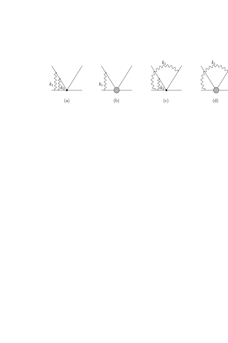
Figure 18: (a) Diagram 1a, (b) representation of diagram 1a in the hard-soft region, (c) diagram 4a, (d) representation of diagram 4a in the hard-soft region.

Diagrams 1a-7b:

We start by considering diagrams 1a-7b. As an example consider diagram 1a, which we redraw in Fig. 18a. This has a potentially non-factorizing contribution from the hard-soft region in which the inner loop is hard (i.e. $k_{2}$ is hard) and the external loop is soft (i.e. $k_{1}$ is soft). The key point is that we can neglect $k_{1}$ in the inner loop, allowing us, in this region of phase space, to represent diagram 1a as in Fig. 18b. The grey circle represents the inner loop (which contains the integral over $k_{2}$, see Fig. 19), but is independent of $k_{1}$. Similarly for diagram 4a, which we redraw in Fig. 18c, the contribution from the region in which $k_{1}$ is soft but $k_{2}$ is hard can be represented as in Fig. 18d, where the grey circle represents the same factor as in Fig. 18b (see Fig. 19). The cancellation of the hard-soft contributions from diagrams 1a and 4a now follows in the same way as for the infra-red divergences in one-loop graphs in Sect. 4.2.

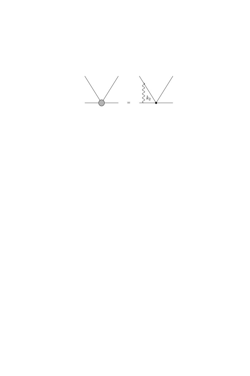
Figure 19: Representation of the hard inner loop.

Similarly the pairs of diagrams {1b, 4b}, {1c, 3a}, {1d, 3b}, {5a, 7b}, {5b, 7b}, {6a, 7a} and {6b, 7a} each cancel by the same argument. Diagrams 7a and 7b appear twice since they each contain two divergent hard-soft contributions (each of the two gluons may be soft). Diagrams 2a-d have no divergent hard-soft contributions.

Diagrams 9a,b, 11a,b and 14a-d:

By inspection we see that diagrams 9a,b, 11a,b and 14a-d have no divergent contributions in the hard-soft region.

Diagrams 10a-d, 15a-d, 16a-d, 18a-d and 19a-d:

The singular terms from the hard-soft contributions from each of the pairs of diagrams {10a, 10c}, {10b, 10d}, {15a, 15b}, {15c, 15d}, {16a, 16b}, {16c, 16d}, {18a, 18b}, {18c, 18d}, {19a, 19b} and {19c, 19d} cancel by the one-loop mechanism as described above. In each case the singular contribution comes from the region of phase space in which the gluon attached to one of the constituents of the pion is soft (in diagrams 15a-d it is the gluon which is attached to both a light and a heavy quark).

Diagrams 17a-d:

We now turn to diagrams 17a-d. In this case the contribution from the region in which the gluon attached to a light quark is soft and the other one is hard does not give a singular contribution. On the other hand, the region in which the gluon attached at both ends to heavy quarks is soft and the other one is hard does lead to singular contributions, which do not cancel, but which are necessary for the validity of the factorization formula. In other words, this contribution does not lead to a singular term in the hard-scattering kernel $T$, but is absorbed into the form-factor.

To see this, observe that the momentum of the soft gluon can be neglected in the hard subgraph. Hence the four diagrams 17a-d contain the diagrams in Fig. 6 as hard subgraph. Since, according to (108), these give $T^{(1)}$, the contribution of diagrams 17a-d to the two-loop $B\to D\pi$ amplitude $A^{(2)}$ in the hard-soft region is of the form

$$A^{(2)}_{\rm 17a-d,hard-soft}=f_{B\to D}^{(1)}\cdot T^{(1)}*\Phi_{\pi}^{(0)},$$ (114)

where $f_{B\to D}^{(1)}$ stands for the soft contribution to the diagram shown in Fig. 20. The factor $f_{B\to D}^{(1)}$ contains non-cancelling infrared divergences. But this factor is identical to the soft contribution to the $B\to D$ form factor $F_{B\to D}^{(1)}$ and hence

$$A^{(2)}_{\rm 17a-d,hard-soft}-F_{B\to D}^{(1)}\cdot T^{(1)}*\Phi_{\pi}^{(0)}=\mbox{ infrared finite}.$$ (115)

Hence we have recovered (and “used up”) one of two subtraction terms that appear in (110). Any other non-cancelling divergence that we may (and must) still find must therefore be cancelled by $F_{B\to D}^{(0)}\cdot T^{(1)}*\Phi_{\pi}^{(1)}$.

Figure 20: One-loop contribution to the $b\to c$ transition form-factor (and hence to $F_{B\to D}$)

Diagrams 8a-d, 12a-d, 13a-d:

We are now left with diagrams 8a-d, 12a-d and 13a-d representing vertex and self-energy insertions on the valence quarks in the pion. A potentially non-factorizing (infrared divergent) contribution arises when the gluon that attaches to the heavy quark line is soft. In order to facilitate the discussion we draw and label these insertions as in Fig. 21. The insertion of Fig. 21a contains a factor

$$\ref{fig:inserts}\mbox{a}=\frac{\gamma^{\mu}(u\not\!q+\not l)\gamma^{\rho}(u\not\!q+\not\!k+\not l)\gamma_{\mu}(u\not\!q+\not\!k)\Gamma}{(uq+l)^{2}\,(uq+k+l)^{2}\,(uq+k)^{2}\,l^{2}}\simeq\frac{\gamma^{\mu}(u\not\!q+\not l)\gamma^{\rho}(u\not\!q+\not l)\gamma_{\mu}}{\left[(uq+l)^{2}\right]^{2}\,l^{2}}\,\,\frac{\not\!q\,\Gamma}{2q\cdot k},$$ (116)

where we have used the fact that the components of $k$ are small with respect to the remaining momenta. This is multiplied by the colour factor $c_{a}=-1/2N_{c}$. In the same region of phase-space the corresponding factor from the diagram in Fig. 21(c) is $c_{c}=N_{c}/2$ times

21c $$\simeq (l_{\mu}g_{\nu\rho}+l_{\nu}g_{\mu\rho}-2l_{\rho}g_{\mu\nu})\,\frac{\gamma^{\mu}\,(u\not\!q+\not l)\gamma^{\nu}}{(uq+l)^{2}\,\left[l^{2}\right]^{2}}\,\frac{\not\!q\,\Gamma}{2q\cdot k}$$ (117)

$$= \frac{2q^{\rho}\,\Gamma}{\left[l^{2}\right]^{2}\,q\cdot k}-2l_{\rho}\frac{\gamma^{\mu}(u\not\!q+\not l)\gamma_{\mu}}{(uq+l)^{2}\,\left[l^{2}\right]^{2}}\,\,\frac{\not\!q\,\Gamma}{2q\cdot k}.$$

The first term on the right-hand side of (117) cancels with the corresponding contribution from diagram 21f and hence we do not consider it further here.

Figure 21: The six vertex and self-energy insertions on the constituents of the pion.

Finally we turn to the self-energy insertion in Fig. 21b,

$$\ref{fig:inserts}\mbox{b}=\frac{\gamma^{\rho}(u\not\!q+\not\!k)\left[(u\not\!q+\not\!k)\Sigma\right](u\not\!q+\not\!k)\Gamma}{\left[(uq+k)\right]^{2}}=\frac{\gamma^{\rho}\Sigma\ (u\not\!q+\not\!k)\Gamma}{(uq+k)^{2}},$$ (118)

where the self-energy $\Sigma$ is given by

$$\int_{l}\frac{\gamma^{\mu}\,(u\not\!q+\not\!k+\not l)\gamma_{\mu}}{(uq+k+l)^{2}\,l^{2}}=(u\not\!q+\not\!k)\Sigma.$$ (119)

In (119) $\int_{l}$ represents the integration over loop momentum $l$. The terms above are to be multiplied by the colour factor $c_{b}=(N_{c}^{2}-1)/2N_{c}$. Differentiating both sides of (119) with respect to $(uq+k)_{\rho}$ we obtain:

$$-\int_{l}\frac{\gamma^{\mu}\,(u\not\!q+\not\!k+\not l)\,\gamma^{\rho}\,(u\not\!q+\not\!k+\not l)\,\gamma_{\mu}}{\left[(uq+k+l)^{2}\right]^{2}\,l^{2}}=\gamma^{\rho}\Sigma+2(uq+k)^{\rho}(u\not\!q+\not\!k)\frac{d\Sigma}{d(uq+k)^{2}}.$$ (120)

Now in this paragraph we are only considering the contribution from the integral over the region of hard $l$. In this case $\Sigma$ is analytic in $(uq+k)^{2}$ and does not have a logarithmic singularity in $(uq+k)^{2}$ at small $(uq+k)^{2}$, so the second term on the right-hand side of (120) is of higher order in $(uq+k)^{2}\ll m_{b}^{2}$ and hence can be neglected. Inserting the expression (120) for $\gamma^{\rho}\Sigma$ into (118) and keeping only the terms which give a singularity from the infrared region of the integration over $k$ we obtain

$$\ref{fig:inserts}\mbox{b}=-\frac{\gamma^{\mu}(u\not\!q+\not l)\gamma^{\rho}(u\not\!q+\not l)\gamma_{\mu}}{\left[(uq+l)^{2}\right]^{2}\,l^{2}}\,\,\frac{\not\!q\,\Gamma}{2q\cdot k},$$ (121)

which apart from the colour factor is minus the contribution from the diagram of Fig. 21a as expected from the Ward identity.

Thus we have two different integrals over $l$ to consider. The first is the one which appears in diagrams 21a and 21b:

$$J_{1}^{\rho}\equiv\int_{l}\frac{\gamma^{\mu}(u\not\!q+\not l)\gamma^{\rho}(u\not\!q+\not l)\gamma_{\mu}}{\left[(uq+l)^{2}\right]^{2}\,l^{2}}=A_{1}\,\gamma^{\rho}+A_{2}\,\not\!q\,q^{\rho},$$ (122)

and the second comes from diagram 21c:

$$J_{2}^{\rho}\equiv\int_{l}\frac{-2l_{\rho}\,\gamma^{\mu}(u\not\!q+\not l)\gamma_{\mu}}{(uq+l)^{2}\,\left[l^{2}\right]^{2}}=B_{1}\,\gamma^{\rho}+B_{2}\,\not\!q\,q^{\rho}.$$ (123)

Since the $\not\!q\,q^{\rho}$ gives zero when multiplied by $\not\!q\,\Gamma/(2q\cdot k)$, the total contribution from 21a-c (up to the term in (117), which cancels with 21f) is

$$21\mbox{a}+21\mbox{b}+21\mbox{c(part)}=\left[(c_{a}-c_{b})A_{1}+c_{c}B_{1}\right]\,\frac{\not\!q\,\Gamma}{2q\cdot k}.$$ (124)

But multiplying $J_{i}^{\rho}$ by $\gamma_{\rho}$ and using the on-shell condition and $q^{2}=0$ gives

$$A_{1}=B_{1}=\int_{l}\frac{1}{l^{2}\,(uq+l)^{2}},$$ (125)

and thus the total contribution is proportional to the combination of colour factors $c_{a}-c_{b}+c_{c}=0$.

Similarly the soft-hard singularity from figures 21d, 21e and the remaining contribution from 21f cancel. Thus we have demonstrated the cancellation of the singularities from the soft-hard region of phase space in each of the sets of six diagrams {8a, 8c, 12a, 12b, 13a, 13c} and {8b, 8d, 12c, 12d, 13b, 13d}. This completes our proof that the contributions from this region of phase-space satisfy the factorization formula.

5.4 The collinear-collinear contribution

We now consider the (logarithmic) singularities from the region of phase space in which the momenta in both loops are collinear with the pion’s momentum. Let $k_{i}$ be the momentum of a gluon collinear with the pion, and write it in terms of Sudakov (light-cone) variables,

$$k_{i}=\alpha_{i}q+\beta_{i}\bar{q}+k_{\perp,i},$$ (126)

with $\bar{q}$ a second light-like vector such that $q\cdot\bar{q}\sim m_{b}^{2}$ (e.g. in a frame in which $q=E\,(1,0,0,1)$, where $E$ is the energy of the pion in the B-meson rest-frame, it is convenient to define $\bar{q}=E\,(1,0,0,-1))$. $k_{\perp,i}$ contains only components which are perpendicular to both $q$ and $\bar{q}$. By “collinear” we mean that $\alpha_{i}\sim 1,\,\beta_{i}\sim\lambda^{2},\,k_{\perp,i}\sim\lambda m_{b}$, with $\lambda\sim\Lambda_{\rm QCD}/m_{b}\ll 1$, and hence $k^{2}\sim\lambda^{2}m_{b}^{2}$. The loop integration measure scales as $d^{4}k_{i}\sim\lambda^{4}m_{b}^{4}$ for collinear $k_{i}$.

Figure 22: The six insertions of two gluons onto the heavy-quark propagators. The momenta $k_{i}$ are parallel to the pion’s momentum $q$ and so we write $k_{i}\approx\alpha_{i}q$. The black circle represents the heavy-quark weak current.

Diagrams 1a-7b:

We start with diagrams 1a-7b, and consider the six ways of attaching two gluons onto the heavy-quark propagators as illustrated in Fig. 22. The heavy quarks are off-shell in this region of phase space and hence their propagators are not singular, which significantly simplifies the discussion. Furthermore, the singularity is at most logarithmic and hence we may approximate the collinear momenta by $k_{i}\approx\alpha_{i}\,q$ ($i=1,2$). The diagrams in Fig. 22 have two Lorentz indices $\mu_{1}$ and $\mu_{2}$ for the external gluon lines. After approximating $k_{i}\approx\alpha_{i}\,q$, the remainder of a diagram, i.e. the light quark lines with their couplings to the two gluons, depends only on the vector $q$, hence the open indices in the diagrams of Fig. 22 must be contracted with $q^{\mu_{1}}q^{\mu_{2}}$. Including this factor, we obtain by repeated use of the on-shell condition for the $b$ quark:

Fig.22a $$= \frac{1}{\alpha_{1}\alpha_{2}}\,\Gamma\,\frac{1}{\not\!p+\alpha_{1}\not\!q+\alpha_{2}\not\!q-m_{b}}\,\alpha_{2}\not\!q\,\frac{1}{\not\!p+\alpha_{1}\not\!q-m_{b}}\,\alpha_{1}\not\!q$$ (127)

$$= \frac{1}{\alpha_{1}\alpha_{2}}\,\Gamma\,\frac{1}{\not\!p+\alpha_{1}\not\!q+\alpha_{2}\not\!q-m_{b}}\,\alpha_{2}\not\!q\,\,=\,\,\frac{1}{\alpha_{1}(\alpha_{1}+\alpha_{2})}\,\Gamma$$

Similar simplifications occur for the other five terms shown in Fig. 22. The relative factors of the six insertions in Fig. 22 are:

Fig.22a $$= \frac{1}{\alpha_{1}\,(\alpha_{1}+\alpha_{2})}\,C_{1}\qquad\textrm{Fig.}~{}\ref{fig:colcol}\mbox{b}\,\,=\,\,\frac{1}{\alpha_{2}\,(\alpha_{1}+\alpha_{2})}\,C_{2}$$ (128)

Fig.22c $$= \frac{1}{\alpha_{2}\,(\alpha_{1}+\alpha_{2})}\,C_{1}\qquad\textrm{Fig.}~{}\ref{fig:colcol}\mbox{d}\,\,=\,\,\frac{1}{\alpha_{1}\,(\alpha_{1}+\alpha_{2})}\,C_{2}$$ (129)

Fig.22e $$= -\frac{1}{\alpha_{1}\,\alpha_{2}}\,C_{2}\qquad\qquad\,\,\textrm{Fig.}~{}\ref{fig:colcol}\mbox{f}\,\,=\,\,-\frac{1}{\alpha_{1}\,\alpha_{2}}\,C_{1}.$$ (130)

$C_{1}$ and $C_{2}$ are the two distinct colour factors, $C_{1}=\textrm{Tr}(T\,T_{2}\,T_{1})$ ($C_{2}=\textrm{Tr}(T\,T_{1}\,T_{2}$)) where $T,\,T_{1}$ and $T_{2}$ are the colour matrices of the heavy-quark weak current and the gluons with momenta $k_{1}$ and $k_{2}$, respectively. Adding up the contributions in (128)-(130) we see that the coefficients of both $C_{1}$ and $C_{2}$ vanish. In this way the singularities from the collinear-collinear region of phase space in the 18 diagrams 1a-7b cancel in each of the following sets of six diagrams {1a, 2a, 2d, 1d, 5a, 6a}, {2c, 1c, 1b, 2b, 5b, 6b} and {3a, 4a, 3b, 4b, 7a, 7b}.

Diagrams 10a-11b:

A similar cancellation occurs for the the six diagrams 10a-11b, which are also individually logarithmically divergent. Indeed the cancellation occurs in each of the two sets of three diagrams {10a, 10d, 11a} and {10c, 10b, 11b}.

Diagrams 8a-9b and 12a-15d:

The diagrams 8a-9b and 12a-15d require special attention as they each contain five light propagators (either light quark or gluon) which are collinear with the pion and these diagrams are hence potentially quadratically divergent. In each case, however, the numerators are suppressed in the collinear-collinear region, so that the leading divergence is logarithmic. The cancellation of this singularity occurs between pairs of diagrams (such as 8a and 8d or 14a and 14d) in the same way as in the one-loop graphs.

As an example consider the numerator that comes from the light quark lines in diagram 12a,

$$N_{12}\equiv\gamma^{\mu}(u\not\!q+\!\not\!k_{2})\gamma^{\rho}(u\not\!q+\!\not\!k_{1}+\!\not\!k_{2})\gamma_{\mu}(u\not\!q+\!\not\!k_{1})\,\Gamma\sim m_{b}^{3}.$$ (131)

The scaling estimate is the naive scaling estimate, according to which diagram 12a is quadratically divergent, not taking into account cancellations. Inserting the Sudakov decomposition (126) and using only the on-shell condition and $q^{2}=0$, this transforms into

$$N_{12} = (u+\alpha_{2})\,\gamma^{\mu}\!\not\!q\,\gamma^{\rho}(\not\!k_{\perp,1}+\!\not\!k_{\perp,2})\gamma_{\mu}\!\not\!k_{\perp,1}\,\Gamma+(u+\alpha_{1}+\alpha_{2})\,\gamma^{\mu}\!\not\!k_{\perp,2}\gamma^{\rho}\not\!q\,\gamma_{\mu}\!\not\!k_{\perp,1}\,\Gamma$$ (132)

$$\,+\,(u+\alpha_{1})\,\gamma^{\mu}\!\not\!k_{\perp,2}\gamma^{\rho}(\not\!k_{\perp,1}+\!\not\!k_{\perp,2})\gamma_{\mu}\not\!q\,\Gamma\sim\lambda^{2}m^{3}_{b}$$

The two leading powers have cancelled, so that the divergence is at most logarithmic. We can now use that $q\cdot k_{\perp,1}=q\cdot k_{\perp,2}=0$ to commute $\not\!q$ to the left. The result is that

$$N_{12}\sim q^{\rho}.$$ (133)

But the logarithmically divergent terms proportional to $q^{\rho}$ (where $\rho$ is the index that couples the gluon in diagram 12a to the heavy-quark line) cancel pairwise according to the one-loop collinear cancellation mechanism discussed in Sect. 4.2. Similar manipulations apply to all other diagrams 8a-9b and 12b-15d.

Diagrams 16a-19d:

The diagrams 16a-19d are not divergent in the collinear-collinear region and we do not consider them further in this subsection. They do however have a collinear divergence, when the gluon attached to one of the constituents of the pion is collinear with the pion’s momentum, while the other momentum is hard. These divergences will be considered when considering the collinear-hard region of phase-space in Sect. 5.6 below.

This concludes our demonstration that the singularities in diagrams from the collinear-collinear region of phase space cancel and hence do not invalidate the factorization formula.

5.5 The soft-collinear contributions

We now present, in some detail, a demonstration that the singularities in the soft-collinear region of phase space do not invalidate the factorization formula, i.e. that soft-collinear singularities cancel in the sum of all diagrams.

5.5.1 Introduction

We start by explaining more carefully what we mean by both “soft” and “collinear”. Let $l$ be the momentum of a gluon collinear with the pion; we write it in terms of Sudakov variables as in (126), $l=\alpha q+\beta\bar{q}+l_{\perp}$. The scaling of the components of $l$ is as described at the beginning of Sect. 5.4.

Consider now a soft gluon with momentum $k$, by which we mean that all components of $k$ are much smaller than $m_{b}$. It is now important to consider what we mean by “much smaller”. To illustrate this point imagine that we have a diagram with a propagator $1/(uq+l)^{2}$, where $l$ is collinear to the pion’s momentum $q$ as described above. By the power counting introduced above we find that this propagator is of order $1/(\lambda^{2}\,m_{b}^{2})$. Now if in addition we have the radiation of a soft gluon, there may be a propagator such as $1/(uq+l+k)^{2}$. If the components of $k$ are of order $\lambda m_{b}$ then $1/(uq+l+k)^{2}\sim 1/(\lambda\,m^{2}_{b})$ and not of order $1/(\lambda^{2}\,m_{b}^{2})$. In this case $k+l$ is not collinear (as defined above), neither is it soft. Indeed in many of the diagrams there are propagators whose denominators are linear combinations of $q\cdot k,\,q\cdot l$ and $l^{2}$. Since $q\cdot l,l^{2}\sim\lambda^{2}m_{b}^{2}$, it is therefore also necessary to consider the region of phase space in which $q\cdot k\sim\lambda^{2}m_{b}^{2}$, which implies that $k\sim\lambda^{2}m_{b}$. We therefore distinguish the regions of phase-space in which the components of $k$ are of order $\lambda m_{b}$ (which we call “soft”) and where they are of order $\lambda^{2}m_{b}$ (which we call “supersoft”). When $l$ is collinear and $k$ is supersoft, then $k+l$ satisfies the scaling conditions for a collinear momentum. This means that when a loop momentum is collinear, one can classify the set of collinear lines of a graph in terms of one-particle-irreducible subgraphs, just as in the case of hard subgraphs. As far as we know, the only previous discussion of the distinction of soft and supersoft in the context of QCD factorization “proofs” is in [30]. If we think of $\lambda$ as being of order $\Lambda_{\rm QCD}/m_{b}$, one may consider the supersoft region as unphysical, since non-perturbative modifications of the quark and gluon propagators would prevent the momentum from becoming supersoft. On the other hand, the structure of denominators clearly indicates that the infrared singularities of Feynman integrals in dimensional regularization originate from supersoft momentum.

Table 2 contains a summary of the rules for determining the order of the divergence from the soft-collinear and supersoft-collinear regions of phase space. We imagine that the gluons have momenta $k$ and $l$ (and $k\pm l$ if the diagram contains a third gluon) and each propagator scales like $1/\lambda^{\delta}$ in these regions. The table contains the powers $\delta$ for the collinear gluon with momentum $l$, the soft (S) or supersoft (SS) gluon with momentum $k$, the gluon with momentum $k\pm l$ and the light and heavy quarks which radiate these gluons. Thus, for example, if there is a light quark propagator $1/(uq+k+l)^{2}$ in a diagram, then it scales like $1/\lambda$ for $k$ soft and $1/\lambda^{2}$ for $k$ supersoft. For the heavy quarks $1/[(p_{b,c}+k+l)^{2}-m^{2}_{b,c}]$ scales like $\lambda^{0}$ (where $p_{b,c}$ are the momenta of the $b$ and $c$ quarks respectively).

Table 2: The power $\delta$ corresponding to the $1/\lambda^{\delta}$ scaling behaviour of each quark and gluon propagator in the soft-collinear (S) and supersoft-collinear (SS) regions of phase space. $l$ is the momentum collinear to the pion’s momentum $q$ and $k$ is soft or supersoft.

		Gluon	Light quark	Heavy quark
	S	2	1	1
$k$	SS	4	2	2
$l$		2	2	0
	S	1	1	0
$k\pm l$	SS	2	2	0

To illustrate the use of the entries in Table 2 consider diagram 1a in Fig. 15 and start with the region in which one gluon is supersoft and the other is collinear. The phase space for this region is of $O(\lambda^{12})$. One possibility is that the outer gluon is supersoft and the inner one is collinear in which case we obtain factors from the propagators proportional to:

$$\begin{array}[]{cccccc}\displaystyle\frac{1}{\lambda^{4}}&\displaystyle\frac{1}{\lambda^{2}}&\displaystyle\frac{1}{\lambda^{2}}&\displaystyle\frac{1}{\lambda^{0}}&\displaystyle\frac{1}{\lambda^{2}}&\displaystyle\frac{1}{\lambda^{2}},\\[11.38092pt] \textrm{supersoft}&\textrm{collinear}&\textrm{outer}&\textrm{inner}&\textrm{outer}&\textrm{inner}\\ \textrm{gluon}&\textrm{gluon}&\textrm{heavy quark}&\textrm{heavy quark}&\textrm{light quark}&\textrm{light quark}\end{array}$$ (134)

which combine to give $1/\lambda^{12}$. Thus we have a logarithmic divergence from this region. If instead the outer gluon is collinear and the inner one is supersoft, then the outer heavy-quark propagator scales like $1/\lambda^{0}$ so that the combined scaling factor for all six propagators is $1/\lambda^{10}$ and there is no divergence.

Now consider the region in which $k$ is soft rather than supersoft, and again we illustrate the power counting in diagram 1a of Fig. 15. In this case the phase space is of $O(\lambda^{8})$ and if the outer gluon is the soft one then the propagators scale as:

$$\begin{array}[]{cccccc}\displaystyle\frac{1}{\lambda^{2}}&\displaystyle\frac{1}{\lambda^{2}}&\displaystyle\frac{1}{\lambda}&\displaystyle\frac{1}{\lambda^{0}}&\displaystyle\frac{1}{\lambda}&\displaystyle\frac{1}{\lambda},\\[11.38092pt] \textrm{soft}&\textrm{collinear}&\textrm{outer}&\textrm{inner}&\textrm{outer}&\textrm{inner}\\ \textrm{gluon}&\textrm{gluon}&\textrm{heavy quark}&\textrm{heavy quark}&\textrm{light quark}&\textrm{light quark}\end{array}$$ (135)

which gives a combined factor of $O(1/\lambda^{7})$. We therefore have no divergence from this region of phase-space (nor from the region in which the inner gluon is the soft one). This is not the case for all the diagrams, however, as we shall demonstrate below.

We now consider the supersoft-collinear and soft-collinear regions in turn.

5.5.2 The supersoft-collinear region

Diagrams 1a-7b

We start by considering the 18 diagrams 1a-7b. We place them into 4 groups {1a, 5a; 2a, 6a; 4a, 7b}, {1b, 5b; 2b, 6b; 4b, 7b}, {1c, 6b; 2c, 5b; 3a, 7a} and {1d, 6a; 2d, 5a; 3b, 7a}. We label these groups I-IV, and only consider explicitly the cancellation within group I (which will require contributions from additional graphs). The cancellations within groups II-IV proceeds analogously to that within group I. Diagrams 5a-7b have two contributions (where the two gluons are supersoft-collinear or collinear-supersoft respectively) and hence appear twice in the lists. Within each group, we identify three pairs (separated by the semicolons). Consider the first pair {1a, 5a} and the region of phase space for which the gluon with the outer vertex on the light quark propagator is the supersoft one (see e.g. Fig. 23a). For the insertion of the singlet-singlet operator $O_{0}$ the singularities from these diagrams cancel analogously to the cancellation of collinear divergences at one-loop level. A similar cancellation occurs between the singularities in all the pairs of diagrams for the insertion of the operator $O_{0}$.

Figure 23: Supersoft-collinear contributions to diagrams 1a [(a)], 2a [(b)] and 4a [(c)]. The gluon labelled by $l$ is collinear with the pion’s momentum $q$ and the one labelled by $k$ is supersoft.

For the insertion of the octet-octet operator $O_{8}$ the cancellation of the singularities is not complete within the set of diagrams 1a-7b. For illustration consider the first group of diagrams {1a, 5a; 2a, 6a; 4a, 7b}. Since, apart from the colour factors, the contributions of the two diagrams in each of the three pairs are equal and opposite, and using the colour factors tabulated in Table 1 the total contribution from this group of diagrams can be written in the form

$$\frac{C_{F}}{2}\,\frac{N_{c}}{2}\,\left(\textrm{Diag1a}-\textrm{Diag2a}+\textrm{Diag4a}\right).$$ (136)

We therefore need to look at diagrams 1a, 2a and 4a in some more detail (see Fig. 23). In this region of phase-space it is straightforward to establish that the integrands are proportional to

Diag1a $$\equiv \frac{2(u+\alpha)}{\alpha}\ \frac{p_{b}\cdot q}{(p_{b}\cdot k)\,(q\cdot k)}\ \frac{1}{k^{2}\,l^{2}\,(uq+k+l)^{2}}$$ (137)

Diag2a $$\equiv \frac{4(u+\alpha)^{2}}{\alpha}\ \frac{p_{b}\cdot q}{p_{b}\cdot k}\ \frac{1}{k^{2}\,l^{2}\,(uq+l)^{2}\,(uq+k+l)^{2}}$$ (138)

Diag4a $$\equiv -\frac{2(u+\alpha)}{\alpha}\ \frac{p_{b}\cdot q}{(p_{b}\cdot k)\,(q\cdot k)}\ \frac{1}{k^{2}\,l^{2}\,(uq+l)^{2}}.$$ (139)

Now using

$$(uq+k+l)^{2}-(uq+l)^{2}\simeq 2(u+\alpha)q\cdot k$$ (140)

we see that $\mbox{Diag2a}=-(\mbox{Diag1a}+\mbox{Diag4a})$ and that the non-cancelling contribution is proportional to the integral over

$$A_{1}=\frac{N_{c}}{2}\ \frac{4(u+\alpha)}{\alpha}\ \frac{p_{b}\cdot q}{(p_{b}\cdot k)(q\cdot k)k^{2}l^{2}}\left(\frac{1}{(uq+k+l)^{2}}-\frac{1}{(uq+l)^{2}}\right),$$ (141)

where we have included the colour factor. Note that here and in the following we do not include explicitly the colour factor $C_{F}/2$ present in one-loop diagrams.

Diagrams 16a-19d:

We now consider diagrams 16a-19d in the supersoft-collinear region. By inspection (power counting) we readily deduce that diagrams 16a-d and 19a-d do not give a singular contribution in this region of phase space, regardless of which of the two gluons is supersoft and which is collinear.

Diagram 17a does have a singular contribution from the region in which the gluon which is attached (at one end) to a light quark is collinear and the one which is attached at both ends to heavy quarks is supersoft. This singularity is cancelled by the corresponding one in diagram 17c by the same mechanism by which collinear divergences cancel at one-loop order (diagrams 17a and 17c have the same colour factor). Similarly the singular contributions from diagrams 17b and 17d cancel.

Diagram 18a has a singular contribution from the region in which the gluon which is attached at one end to a light quark is supersoft and the one which is attached at both ends to the $b$ quark is collinear. This singularity cancels against the corresponding one in diagram 18b, by the same mechanism by which soft divergences cancel at one-loop order. Similarly the singularities in diagrams 18c and 18d cancel.

Thus there is no residual singular contribution from diagrams 16a-19d.

Diagrams 10a-11b:

We now turn to the six diagrams 10a-11b. Consider diagram 10a and the three collinear-supersoft contributions as labelled in Fig. 24. The propagators in the region of Fig. 24a combine to give a factor of $\lambda^{-10}$ and hence no singularity. In the regions of Fig. 24b and Fig. 24c, however, they give factors of $\lambda^{-12}$ and hence do yield singular contributions. The singular contribution from the region in Fig. 24c can readily be seen to cancel the corresponding contribution from diagram 10c by the standard mechanism of one-loop soft cancellations. This leaves us the contribution of Fig. 24b, which is straightforward to evaluate giving a term proportional to the integral over

$$\textrm{Diag10a}\equiv-2(u+\alpha)\ \frac{p_{b}\cdot q}{p_{b}\cdot k}\ \frac{1}{k^{2}l^{2}(k+l)^{2}(uq+k+l)^{2}},$$ (142)

where we have used a shift of integration variable $l\to l+k$. The corresponding contributions from diagrams 10b, 10c and 10d contribute to groups II, III and IV respectively.

Figure 24: The three possible momentum routings in the supersoft-collinear region for diagrams 10a [(a)-(c)] and 11a [(d)-(f)]. $l$ represents the collinear momentum and $k$ the supersoft one.

Consider now diagram 11a and consider the three regions of phase-space as labelled in Fig. 24d-f. The region in Fig. 24f does not give a singular contribution, whereas the other two regions do. We consider the contribution from Fig. 24d here, that from Fig. 24e contributes to group IV. Similarly the two singular contributions from diagram 11b contribute to groups II and III. The contribution from the region in Fig. 24d can readily be evaluated and is proportional to the integral over

$$\textrm{Diag11a(part)}\equiv 2(u+\alpha)\ \frac{p_{b}\cdot q}{p_{b}\cdot k}\ \frac{1}{k^{2}l^{2}(k+l)^{2}(uq+k+l)^{2}},$$ (143)

where we repeat that it is only the part of diagram 11a which contributes to group I which is being evaluated.

Putting in the colour factor of $N_{c}/2$ for diagram 10a ($-N_{c}/2$ for diagram 11a) and summing the contributions from (142) and (143), we obtain a singular contribution to group I of

$$A_{2}=-\frac{N_{c}}{2}\ 4(u+\alpha)\ \frac{p_{b}\cdot q}{p_{b}\cdot k}\ \frac{1}{k^{2}l^{2}(k+l)^{2}(uq+k+l)^{2}}.$$ (144)

Next we note that $(k+l)^{2}\approx l^{2}+2\alpha q\cdot k$ so that

$$1=\frac{(k+l)^{2}}{2\alpha q\cdot k}-\frac{l^{2}}{2\alpha q\cdot k}$$ (145)

and

$$A_{2} = \frac{N_{c}}{2}\,(-2)\,\frac{(u+\alpha)}{\alpha}\ \frac{p_{b}\cdot q}{(p_{b}\cdot k)(q\cdot k)k^{2}l^{2}}\ \left(\frac{1}{(uq+k+l)^{2}}-\frac{1}{(uq+l)^{2}}\right)$$ (146)

$$= -\frac{1}{2}\,A_{1}$$ (147)

where we have made the change of variables $l\to l-k$ in the second term of (146). (Since $l-k$ remains collinear for supersoft $k$, this change of variables is permitted for supersoft $k$, but would not be permitted for soft $k$.)

Diagrams 8a-9b and 12a-15d:

Finally we consider the remaining diagrams in which there is a single gluon attached (at one end) to one of the heavy quarks. Power counting (including the momentum factor in the numerator) shows that there is no singularity when this gluon is collinear. Thus we can restrict our attention to the region in which the gluon which is attached to the heavy quark is supersoft. Note that in this case the superficial degree of divergence is quadratic. However, taking the numerator factors into account, the actual divergence is again only logarithmic as can be seen from the expressions below.

Consider the contributions to diagrams 8a, 12a and 13a from this region of phase space. This contribution can be written in the form:

$$A_{3}=\frac{N_{c}}{2}\,\textrm{Diag8a}+\left(\frac{-1}{2N_{c}}\right)\,\textrm{Diag12a}+\left(\frac{N_{c}}{2}-\frac{1}{2N_{c}}\right)\,\textrm{Diag13a},$$ (148)

where we have explicitly exhibited the colour factors. Straightforward evaluation of the diagrams shows that they are respectively proportional to the integrals over

Diag8a $$\equiv \frac{4\alpha q\cdot(k+l)+2(u+\alpha)q\cdot k+2(uq+l)^{2}}{(uq+k+l)^{2}k^{2}l^{2}(k+l)^{2}}\ \frac{p_{b}\cdot q}{(p_{b}\cdot k)(q\cdot k)}$$ (149)

Diag12a $$\equiv \frac{2l_{\perp}^{2}}{(uq+l)^{2}(uq+k+l)^{2}k^{2}l^{2}}\ \frac{p_{b}\cdot q}{(p_{b}\cdot k)(q\cdot k)}$$ (150)

Diag13a $$\equiv \frac{-2q\cdot(l+k)}{(uq+l+k)^{2}k^{2}l^{2}}\ \frac{p_{b}\cdot q}{(p_{b}\cdot k)(q\cdot k)^{2}},$$ (151)

where in (150) we use a metric such that $l_{\perp}^{2}$ is negative.

Using $l_{\perp}^{2}=(uq+l)^{2}-2(u+\alpha)q\cdot l$, $2(u+\alpha)q\cdot k=(uq+k+l)^{2}-(uq+l)^{2}$, and dropping a term that vanishes after integration over $k$ because it is antisymmetric in $k$, one readily finds that $\mbox{Diag12a}=-\mbox{Diag13a}$, so that (148) becomes

$$A_{3}=\frac{N_{c}}{2}(\textrm{Diag8a}-\textrm{Diag12a}).$$ (152)

Similarly using (145) we find that the first term in the numerator of (149) for diagram 8a gives the same contribution as diagram 12a, so that $A_{3}$ is the sum of the contributions of the second and third terms in the numerator of (149):

$$A_{3} = \frac{N_{c}}{2}\ \frac{2(u+\alpha)q\cdot k+2(uq+l)^{2}}{(uq+k+l)^{2}k^{2}l^{2}(k+l)^{2}}\ \frac{p_{b}\cdot q}{(p_{b}\cdot k)(q\cdot k)}$$ (153)

$$= \frac{N_{c}}{2}\ \frac{2(uq+k+l)^{2}-2(u+\alpha)q\cdot k}{(uq+k+l)^{2}k^{2}l^{2}(k+l)^{2}}\ \frac{p_{b}\cdot q}{(p_{b}\cdot k)(q\cdot k)}$$ (154)

$$= \frac{N_{c}}{2}\ \left\{\frac{2}{k^{2}l^{2}(k+l)^{2}}-\frac{2(u+\alpha)q\cdot k}{(uq+k+l)^{2}k^{2}l^{2}(k+l)^{2}}\right\}\ \frac{p_{b}\cdot q}{(p_{b}\cdot k)(q\cdot k)}.$$ (155)

The first term in the braces in (155) is independent of $u$. It cancels against the corresponding term in diagram 8c by the standard one-loop soft cancellation mechanism and so we drop it from the definition of $A_{3}$. We are left with the second term which (by direct comparison with the expression in (144) ) gives

$$A_{3}=\frac{1}{2}\,A_{2}.$$ (156)

We do not exhibit all the corresponding formulae here for diagrams 9a, 14a and 15a but the steps are very similar. There is one subtlety in that diagram 9a has two contributions, one to group I and the other to group III. Keeping only the part which has the right structure to be of group I we find

$$A_{4} = \frac{N_{c}}{2}\textrm{Diag9a(part)}+\left(\frac{N_{c}}{2}-\frac{1}{2N_{c}}\right)\textrm{Diag14a}+\left(-\frac{1}{2N_{c}}\right)\textrm{Diag15a}$$ (157)

$$= \frac{1}{2}\,A_{2}.$$

The evaluation of the contributions to the remaining groups of diagrams proceeds in a similar way. Group II has contributions from diagrams {8b, 9b(part), 12d, 13b, 14b, 15c}, group III from {8c, 9a(part), 12b, 13c, 14c, 15b} and group IV from {8d, 9b(part), 12c, 13d, 14d, 15d}.

Total:

The total contribution in group I is $A_{1}+A_{2}+A_{3}+A_{4}$, where $A_{3}=A_{4}=A_{2}/2$ (see (156) and (157)) and $A_{1}=-2A_{2}$ (see (147)). Thus the total contribution in group I is zero. The cancellation of all the contributions to groups II, III and IV occurs in a similar way. Hence we have demonstrated that there are no infrared singularities in the supersoft-collinear region of phase-space.

5.5.3 The soft-collinear region

We also discuss briefly how the cancellation of singular contributions occurs in the soft-collinear case. This case is simpler than the supersoft-collinear case, since some terms that contribute to singularities for supersoft $k$ give convergent integrals for soft $k$, while the converse never occurs. As a consequence we shall see that the soft-collinear case is covered by the line of argument that applied to the supersoft-collinear case.

Diagrams 1a-7b:

By power counting we see that the diagram 1a has no singular contribution in the soft-collinear region, whereas diagrams 2a and 4a do. Thus

$$A_{1\ \textrm{\scriptsize{soft}}}=\frac{N_{c}}{2}\,(-\textrm{Diag2a+Diag4a}).$$ (158)

Using the relation $(uq+k+l)^{2}\simeq 2(u+\alpha)q\cdot k$ which is valid in the soft-collinear region, we find that Diag2a = $-$Diag4a and

$$A_{1\ \textrm{\scriptsize{soft}}}=-4\frac{N_{c}}{2}\frac{u+\alpha}{\alpha}\ \frac{p_{b}\cdot q}{(p_{b}\cdot k)(q\cdot k)}\ \frac{1}{k^{2}l^{2}(uq+l)^{2}}.$$ (159)

Diagrams 16a-19d:

Diagrams 16a and 19a are convergent in this region of phase space just as they were in the supersoft-collinear one. Diagram 18a, which is singular in the supersoft-collinear region is now convergent.

Diagram 17a does have a singular contribution again, from the region in which the gluon which is attached (at one end) to a light quark is collinear and the one which is attached at both ends to heavy quarks is soft. As above, this singularity is cancelled by the corresponding one in diagram 17c by the same mechanism by which collinear divergences cancel at one-loop order (diagrams 17a and 17c have the same colour factor). Similarly the singular contributions from diagrams 17b and 17d cancel. Thus there is no residual singular contribution from diagrams 16a-19d.

Diagrams 10a-11b:

Consider diagram 10a and the momentum routings exhibited in Fig. 24. Power counting now indicates that only the routing of Fig. 24b gives a singular contribution and this can readily be evaluated:

$$\textrm{Diag10a}=-2\frac{N_{c}}{2}(u+\alpha)\ \frac{p_{b}\cdot q}{p_{b}\cdot k}\ \frac{1}{k^{2}l^{2}(k-l)^{2}(uq+l)^{2}}.$$ (160)

There is a singular contribution from the diagram 11a from the routing in Fig. 24d (the routing in Fig. 24e is also singular but contributes to group IV). Explicit evaluation of this contribution shows that it is equal to that in (160), so that the combined contribution from diagrams 10a and the part of diagram 11a which contributes to group I is

$$A_{2\ \textrm{\scriptsize{soft}}}=-4\frac{N_{c}}{2}(u+\alpha)\ \frac{p_{b}\cdot q}{p_{b}\cdot k}\ \frac{1}{k^{2}l^{2}(k-l)^{2}(uq+l)^{2}}.$$ (161)

In the soft collinear region $(k-l)^{2}\simeq-2\alpha q\cdot k$, so that

$$A_{2\ \textrm{\scriptsize{soft}}}=-\frac{1}{2}\,A_{1\ \textrm{\scriptsize{soft}}}$$ (162)

as in the supersoft-collinear case.

Diagrams 8a-9b and 12a-15d:

We start by considering diagrams 8a, 12a and 13a in the soft collinear region. In general, and for 13a in particular, when the gluon which is attached to a heavy quark is collinear, the cancellation of the corresponding singularity proceeds in an analogous way to the cancellation of one-loop collinear divergences. In fact for some diagrams (such as 8a or 12a) the potentially divergent contribution vanishes by itself. This leaves us to consider the contributions when this gluon is soft. Although by power counting it may appear that diagrams 12a and 13a are logarithmically or linearly divergent, the numerators of these diagrams vanish sufficiently quickly to render them finite. This leaves us with the singularity in diagram 8a from the region sketched in Fig. 25a which has to be evaluated and is found to be

$$\textrm{Diag8a}=-2\frac{N_{c}}{2}(u+\alpha)\ \frac{p_{b}\cdot q}{p_{b}\cdot k}\ \frac{1}{k^{2}l^{2}(k-l)^{2}(uq+l)^{2}}.$$ (163)

Therefore we have

$$A_{3\ \textrm{\scriptsize{soft}}}=\frac{1}{2}\,A_{2\ \textrm{\scriptsize{soft}}}$$ (164)

as before.

Figure 25: Momentum routings for diagrams 8a and 9a which are considered in the text for $l$ collinear to the pion and $k$ soft.

Finally we have to consider diagrams 14a, 15a and the part of diagram 9a which contributes to group I. The contribution to diagram 14a from the region in which the gluon which is attached to a heavy quark is soft, is superficially quadratically divergent, but the numerator reduces the divergence to a logarithmic one. This singularity is cancelled by the analogous one in diagram 14c by the standard mechanism for the cancellation of soft singularities at one-loop order. The remaining terms in diagram 14a are finite. Diagram 15a is superficially linearly divergent, but the numerators render it finite. This leaves the contribution from the diagram 9a to group I, as sketched in Fig. 25b. This can be evaluated and is found to be

$$\textrm{Diag6a}=-4\frac{N_{c}}{2}(u+\alpha)(\bar{u}-\alpha)\ \frac{(p_{b}\cdot q)(q\cdot k)}{p_{b}\cdot k}\ \frac{1}{k^{2}l^{2}(k-l)^{2}(uq+l)^{2}(\bar{u}q-l+k)^{2}}.$$ (165)

But in this region of phase space $(\bar{u}q-l+k)^{2}\simeq 2(\bar{u}-\alpha)\,q\cdot k$, so that again

$$A_{4\ \textrm{\scriptsize{soft}}}=\frac{1}{2}\,A_{2\ \textrm{\scriptsize{soft}}}.$$ (166)

Thus collecting up (162), (164) and (166) as before we find that the total contribution is zero:

$$A_{1\ \textrm{\scriptsize{soft}}}+A_{2\ \textrm{\scriptsize{soft}}}+A_{3\ \textrm{\scriptsize{soft}}}+A_{4\ \textrm{\scriptsize{soft}}}=0.$$ (167)

5.6 The hard-collinear contribution

In this subsection we consider the region in which one loop momentum is collinear with the pion’s momentum and the other is hard. We choose loop momenta such that a gluon has collinear momentum $l$ and write $l=\alpha q+\beta\bar{q}+l_{\perp}$. $k$ denotes a hard momentum and we choose it such that a gluon line has momentum $k$. As in the hard-soft case we can consider one-particle-irreducible hard subgraphs (since adding a collinear momentum to a hard momentum gives a hard momentum). But note that since $\alpha q\sim m_{b}$, the hard subgraph depends on $\alpha$, and a convolution in $\alpha$ with the remainder of the graph remains.

To anticipate the result of this subsection recall that we need to demonstrate that (110) is valid and that we have already identified the second of the two subtraction terms with a non-cancelling divergence in the hard-soft region. In order to verify that (110) is valid, it remains to show that there is a non-cancelling divergence in the hard-collinear region that has the structure of the first subtraction term, $F^{(0)}_{B\to D}\cdot T^{(1)}*\Phi_{\pi}^{(1)}$. It is plausible that we should find this term in the hard-collinear region, since $T^{(1)}$ is the hard one-loop amplitude and $\Phi_{\pi}^{(1)}$ has only collinear divergences.

Diagrams 1a-7b:

It is straightforward to establish that in order to get a divergence the gluon with the collinear momentum must be attached to the end of a light-quark or antiquark line and not internally (see Fig. 26). Since the divergences are logarithmic we can set $l=\alpha q$, and because the collinear gluon is attached to the end of a light-quark or antiquark line we always get (using the on-shell condition) a factor proportional to $q_{\rho}$, where $\rho$ is the Lorentz index of the collinear gluon.

Figure 26: Components of two-loop Feynman diagrams. $l$ is collinear with the pion’s momentum and $k$ is a hard momentum. Routing (a) leads to potentially singular contributions whereas routing (b) does not.

Figure 27: Attachments of the collinear gluon (labelled by $l$) and hard gluon (with momentum $k$) to the heavy quarks (see text).

Consider now the diagrams in which both gluons are attached to the $b$ quark as indicated in Fig. 27a. These are diagrams {1a, 1c, 3a(part), 4a(part)}. These diagrams all contain the factor

$$\Gamma\frac{1}{(\not\!p_{b}+\alpha\not\!q+\not\!k-m_{b})}\gamma^{\mu}\,\frac{1}{(\not\!p_{b}+\alpha\not\!q-m_{b})}\,\alpha\not\!q,$$ (168)

which can be simplified to

$$\Gamma\frac{1}{(\not\!p_{b}+\alpha\not\!q+\not\!k-m_{b})}\gamma^{\mu}.$$ (169)

(Strictly speaking these diagrams contain the factor (168) without the factor $\alpha$. We have included this factor for convenience and correct for it later in (177).)

Similarly consider the diagrams in which the two gluons are attached to the $b$ quark as in Fig. 27b, i.e. diagrams {2a, 2c, 4a(part), 3a(part)}. These all have a factor

$$\Gamma\frac{1}{(\not\!p_{b}+\alpha\not\!q+\not\!k-m_{b})}\,\alpha\not\!q\,\frac{1}{(\not\!p_{b}+\not\!k-m_{b})}\,\gamma^{\mu},$$ (170)

which simplifies to

$$\Gamma\frac{1}{(\not\!p_{b}+\not\!k-m_{b})}\,\gamma^{\mu}\ -\Gamma\frac{1}{(\not\!p_{b}+\alpha\not\!q+\not\!k-m_{b})}\,\gamma^{\mu}.$$ (171)

Apart from the factors in (169) and (171) and the colour factors, the remaining terms are common in the two sets of diagrams in the order we have written them (i.e. the remaining factors in diagram 1a are equal to those in diagram 2a etc.).

Next consider the diagrams which have the hard gluon attached to the $b$ quark and the collinear one to the $c$-quark as in Fig. 27c, i.e. diagrams {6a, 5b, 7b(part), 7a(part)}. These all have a common factor

$$\alpha\not\!q\,\frac{1}{(\not\!p_{c}-\alpha\not\!q-m_{c})}\,\Gamma\,\frac{1}{(\not\!p_{b}+\not\!k-m_{b})}\,\gamma^{\mu},$$ (172)

which can be simplified to

$$-\Gamma\frac{1}{(\not\!p_{b}+\not\!k-m_{b})}\gamma^{\mu}.$$ (173)

Again the remaining factors are equal in each of the four diagrams as in the corresponding diagrams of the previous two sets.

Summing up these contributions we find they are of the form

$$(C_{1}-C_{2})\Gamma\frac{1}{(\not\!p_{b}+\alpha\not\!q+\not\!k-m_{b})}\,\gamma^{\mu}+(C_{2}-C_{3})\Gamma\frac{1}{(\not\!p_{b}+\not\!k-m_{b})}\,\gamma^{\mu},$$ (174)

where $C_{1},C_{2}$ and $C_{3}$ are the remaining terms in each of the three sets of diagrams (they are equal except for the colour factors).

Similarly when the hard gluon couples to the charm quark we obtain

$$(C^{\prime}_{1}-C^{\prime}_{2})\gamma^{\mu}\frac{1}{\not\!p_{c}-\not\!k-m_{c}}\Gamma-(C^{\prime}_{3}-C^{\prime}_{2})\gamma^{\mu}\frac{1}{\not\!p_{c}-\alpha\not\!q-\not\!k-m_{c}}\Gamma.$$ (175)

When we insert the singlet-singlet operator $O_{0}$, all the colour factors are equal and hence $C_{1}-C_{2}=C_{3}-C_{2}=0$ (and similarly for the $C_{i}^{\prime}$) and we get an immediate cancellation. We therefore only need to consider the insertion of the octet-octet operator $O_{8}$. In this case $C^{\prime}_{1}-C_{2}^{\prime}=-(C_{1}-C_{2})$ and $C^{\prime}_{3}-C_{2}^{\prime}=-(C_{3}-C_{2})$ so that these diagrams give a contribution which is the integral over

$$\frac{N_{c}}{2}\Bigg{[}\,\Gamma\left(\frac{1}{\not\!p_{b}+\alpha\not\!q+\not\!k-m_{b}}-\frac{1}{\not\!p_{b}+\not\!k-m_{b}}\right)\,\gamma^{\mu}-$$

$$\hskip 42.67912pt\gamma^{\mu}\left(\frac{1}{\not\!p_{c}-\not\!k-m_{c}}-\frac{1}{\not\!p_{c}-\alpha\not\!q-\not\!k-m_{c}}\right)\Gamma\,\Bigg{]}\,\times{\cal L}$$ (176)

where ${\cal L}$ represents the contributions from the remaining parts of the diagrams, i.e. the gluon propagators and the contribution from the light quark lines, but with a factor $\alpha q^{\rho}$, that has already been included, extracted. Hence ${\cal L}$ is given by

$${\cal L} = \frac{1}{k^{2}l^{2}}\cdot$$ (177)

$$\left[\frac{2(u+\alpha)}{\alpha}\,\frac{\gamma^{\mu}((u+\alpha)\not\!q+\not\!k)\Gamma}{(uq+l)^{2}((u+\alpha)q+k)^{2}}-\frac{2(\bar{u}+\alpha)}{\alpha}\,\frac{\Gamma((\bar{u}+\alpha)\not\!q+\not\!k)\gamma^{\mu}}{(\bar{u}q+l)^{2}((\bar{u}+\alpha)q+k)^{2}}\right.$$

$$\hskip 8.5359pt\left.+\,\frac{2(u+\alpha)}{\alpha}\,\frac{\Gamma(\bar{u}\not\!q+\not\!k)\gamma^{\mu}}{(uq+l)^{2}(\bar{u}q+k)^{2}}-\frac{2(\bar{u}+\alpha)}{\alpha}\,\frac{\gamma^{\mu}(u\not\!q+\not\!k)\Gamma}{(\bar{u}q+l)^{2}\,(uq+k)^{2}}\right].$$

The four terms in square brackets in (177) correspond to the groupings we introduced above, e.g., the diagrams {1a, 1c, 3a(part), 4a(part)} or in the case of the hard gluon being attached to the charm quark they may be {5a, 6b, 7a(part), 7b(part)}. The common factor of $1/\alpha$ in (177) is present because we have already included a factor of $\alpha q^{\rho}$ in the evaluation of the factors from the heavy quarks. This completes the consideration of the contribution from diagrams 1a-7b.

Diagrams 8a-9b:

We now consider diagrams 8a-9b, which have a similar structure for the light quarks as diagrams 1a-7b. Evaluation of these diagrams yields the result

$$\frac{N_{c}}{2}\,\alpha q^{\rho}\left((l-k)_{\nu}g_{\mu\rho}+(2k+l)_{\rho}g_{\mu\nu}-(2l+k)_{\mu}g_{\nu\rho}\right)\cdot$$

$$\hskip 21.68121pt\frac{-1}{(k+l)^{2}}\left(\Gamma\frac{1}{\not\!p_{b}+\not\!k+\not l-m_{b}}\gamma^{\nu}+\gamma^{\nu}\frac{1}{\not\!p_{c}-\not\!k-\not l-m_{c}}\Gamma\right)\,\times{\cal L}.$$ (178)

In the factor coming from the triple gluon vertex in (178) we can approximate $l$ by $\alpha q$, so that

$$q^{\rho}\left((l-k)_{\nu}g_{\mu\rho}+(2k+l)_{\rho}g_{\mu\nu}-(2l+k)_{\mu}g_{\nu\rho}\right)$$

$$\hskip 85.35826pt=(\alpha q-k)_{\nu}q_{\mu}+2q\cdot kg_{\mu\nu}-(2\alpha q+k)_{\mu}q_{\nu}.$$ (179)

Next we make use of the fact that $q_{\mu}$ gives zero when contracted with ${\cal L}$ so that we can drop it and that $(k+l)^{2}=k^{2}+2\alpha q\cdot k$, to write the contribution from these diagrams as

$$\frac{N_{c}}{2}\left\{(k+l)^{2}g_{\mu\nu}-k^{2}g_{\mu\nu}-k_{\mu}\alpha q_{\nu}\right\}\cdot$$

$$\hskip 14.45377pt\frac{-1}{(k+l)^{2}}\left(\Gamma\frac{1}{\not\!p_{b}+\not\!k+\not l-m_{b}}\gamma^{\nu}+\gamma^{\nu}\frac{1}{\not\!p_{c}-\not\!k-\not l-m_{c}}\Gamma\right)\,\times{\cal L}.$$ (180)

We now consider the three terms in { } in (180) in turn. The first term cancels two of the four terms in (176) from diagrams 1a-7b. The remaining two terms in (176) can be combined with the second term in { } in (180) to give

$$X_{1} \equiv \frac{N_{c}}{2}\left(\,\frac{2(u+\alpha)}{\alpha}\frac{1}{(uq+l)^{2}l^{2}}[T(u)-T(u+\alpha)]\right.+$$ (181)

$$\hskip 57.81621pt\left.\frac{2(\bar{u}+\alpha)}{\alpha}\frac{1}{(\bar{u}q+l)^{2}l^{2}}[T(u)-T(u-\alpha)]\right),$$

where

$$T(u)\equiv\frac{1}{k^{2}}\left(\gamma^{\mu}\frac{1}{u\not\!q+\not\!k}\Gamma-\Gamma\frac{1}{\bar{u}\not\!q+\not\!k}\gamma^{\mu}\right)\times\left(\Gamma\frac{1}{\not\!p_{b}+\not\!k-m_{b}}\gamma^{\mu}+\gamma^{\mu}\frac{1}{\not\!p_{c}-\not\!k-m_{c}}\Gamma\right).$$ (182)

Note that $T(u)$ is exactly the integrand for the hard amplitude at one-loop order, i.e. using the notation of (106)

$$\int_{k}T(u)=T^{(1)},$$ (183)

where $\int_{k}$ denotes integration over the loop momentum $k$.

Finally we have to evaluate the third term in { } in (180), which gives a contribution of

$$X_{2} \equiv \frac{N_{c}}{2}\frac{4}{k^{2}l^{2}(k+l)^{2}}\left[\frac{u+\alpha}{\alpha}\frac{1}{(uq+l)^{2}}\Gamma-\frac{\bar{u}+\alpha}{\alpha}\frac{1}{(\bar{u}q+l)^{2}}\,\Gamma\right]\times$$ (184)

$$\left(\Gamma\,\frac{1}{\not\!p_{b}+\alpha\not\!q+\not\!k-m_{b}}\,\alpha\not\!q\,+\,\alpha\not\!q\,\frac{1}{\not\!p_{c}-\alpha\not\!q-\not\!k-m_{c}}\,\Gamma\,\right).$$

$X_{1}+X_{2}$ is the total contribution from diagrams 1a-9b.

Diagrams 12 and 15:

We now consider diagrams 12a-12d and 15a-15d. In these diagrams there are singular contributions when either of the two gluons is collinear (and the other one is hard). However, in the case where the gluon which is attached at one end to one of the heavy quarks is collinear, the standard mechanism for the cancellation of collinear divergences at one-loop level applies (the singularities of diagrams 15a and 15d cancel as do those in each pair of diagrams {15b, 15c}; {12a, 12c} and {12b, 12d}).

Figure 28: Attachments of the collinear gluon (labelled by $l$) and hard gluon (with momentum $k$) to the light quarks, as required for the evaluation of diagrams 12 and 15 (see text).

We therefore need only to consider the case where the collinear gluon is the one attached at both ends to the light quarks. Straightforward evaluation of the factor coming from the light quarks (see Fig. 28) shows that this factor is equal to

$$\frac{2(u+\alpha)}{\alpha}\frac{1}{(uq+l)^{2}}\bigg{(}\gamma^{\mu}\frac{1}{u\not\!q+\not\!k}\Gamma-\gamma^{\mu}\frac{1}{(u+\alpha)\not\!q+\not\!k}\Gamma$$

$$-\Gamma\frac{1}{\bar{u}\not\!q+\not\!k}\gamma^{\mu}+\Gamma\frac{1}{(\bar{u}-\alpha)\not\!q+\not\!k}\gamma^{\mu}\bigg{)}$$

$$+\frac{2(\bar{u}+\alpha)}{\alpha}\frac{1}{(\bar{u}q+l)^{2}}\bigg{(}\gamma^{\mu}\frac{1}{u\not\!q+\not\!k}\Gamma-\gamma^{\mu}\frac{1}{(u-\alpha)\not\!q+\not\!k}\Gamma$$

$$-\Gamma\frac{1}{\bar{u}\not\!q+\not\!k}\gamma^{\mu}+\Gamma\frac{1}{(\bar{u}+\alpha)\not\!q+\not\!k}\gamma^{\mu}\bigg{)}.$$ (185)

But this is exactly the same factor as appears in the expression $X_{1}$ in (181). Indeed, the contribution from diagrams 12 and 15 is identical to (181) except that the colour factor is $-1/2N_{c}$, instead of $N_{c}/2$. Combining the contributions from all the diagrams we have evaluated so far, i.e. diagrams 1a-9b, 12a-12d and 15a-15d, we find a total contribution of $2C_{F}/N_{c}\,X_{1}+X_{2}$.

Figure 29: Momentum routings in (a) diagram 16a, (b) diagram 17a (c) diagram 18a and (d) diagram 19a which are considered in the text. $l$ is a momentum collinear with that of the pion and $k$ is a hard momentum.

Diagrams 16a-19d:

In diagrams 16a-19d, the singular contribution comes from the region in which the collinear gluon is the one attached at one end to the light-quarks. As an example consider the diagram 16a (see Fig. 29a). The factor coming from the heavy-quark lines (again multiplying it by $\alpha q^{\rho}$) is of the form:

Diag16a $$\equiv \Gamma\,\frac{1}{\not\!p_{b}+\alpha\not\!q-m_{b}}\,\gamma^{\mu}\,\frac{1}{\not\!p_{b}+\alpha\not\!q+\not\!k-m_{b}}\,\alpha\not\!q\,\frac{1}{\not\!p_{b}+\not\!k-m_{b}}\,\gamma_{\mu}$$ (186)

$$=\Gamma\,\frac{1}{\not\!p_{b}+\alpha\not\!q-m_{b}}\,\gamma^{\mu}\,\frac{1}{\not\!p_{b}+\not\!k-m_{b}}\,\gamma_{\mu}-\Gamma\,\frac{1}{\not\!p_{b}+\alpha\not\!q-m_{b}}\,\gamma^{\mu}\,\frac{1}{\not\!p_{b}+\alpha\not\!q+\not\!k-m_{b}}\,\gamma_{\mu}$$

$$\equiv a_{1}-a_{2}.$$

The analogous contribution from diagram 17a is

$$\textrm{Diag17a}\equiv\gamma^{\mu}\frac{1}{\not\!p_{c}+\not\!k-m_{c}}\,\Gamma\,\frac{1}{\not\!p_{b}+\not\!k-m_{b}}\,\gamma_{\mu}-a_{3},$$ (187)

where

$$a_{3}\equiv\gamma^{\mu}\,\frac{1}{\not\!p_{c}+\not\!k-m_{c}}\,\Gamma\,\frac{1}{\not\!p_{b}+\alpha\not\!q+\not\!k-m_{b}}\,\gamma_{\mu}.$$ (188)

The first term in (187) cancels against the corresponding contribution from diagram 17c and we do not include it further in the discussion. Finally the corresponding terms in diagrams 18a and 19a are

Diag18a $$= a_{2}$$ (189)

Diag19a $$= a_{3}.$$ (190)

All the remaining factors in these diagrams are the same, apart from the colour factors, so including these we find that the sum of these four diagrams gives a contribution which is proportional to

$$\textrm{Diag16a+Diag17a+Diag18a+Diag19a}=-\frac{1}{2N_{c}}a_{1}+\frac{N_{c}}{2}(a_{2}-a_{3}).$$ (191)

Figure 30: Insertion of a mass-renormalization counterterm into a one-loop diagram.

There is a further subtlety, however, and this concerns the mass renormalization of the $b$ quark (see Fig. 30). The singular contribution does not cancel (in contrast to the wave-function renormalization), and is readily found to be $-C_{F}\,a_{1}$. Thus the contribution of the diagrams {16a, 17a, 18a, 19a} together with that from the diagram with the mass counterterm gives a contribution which is proportional to

$$-\frac{N_{c}}{2}\,(a_{1}-a_{2}+a_{3}).$$ (192)

The remaining diagrams in the set 16a-19d yield analogous results, with different factors from the light quarks naturally.

Diagrams 10a-11b:

Again the only singular contribution comes from the region in which the collinear gluon is the one which is attached at one end to a light quark (see Fig. 24a). Explicit evaluation of diagram 10a gives the following contribution:

$$\textrm{Diag10a}=\frac{N_{c}}{2}(a_{1}-a_{2})\,+\,\frac{N_{c}}{2}\,\frac{1}{(k+l)^{2}}\left[2\Gamma-\Gamma\,\frac{1}{\not\!p_{b}+\alpha\not\!q+\not\!k-m_{b}}\,\alpha\not\!q\,\right],$$ (193)

where all remaining factors are as in the previous paragraph. Thus we see that the first term cancels part of the contribution from diagrams 16a-19d in (192). The term $2\Gamma$ in the square brackets cancels against the corresponding contribution in diagram 10d and we do not consider it further. This leaves us with the second term in square brackets, which cancels half of the corresponding contribution in $X_{2}$ (by corresponding term we mean the product of the first term in the square brackets in (184) with the first term in the brackets on the second line). The remaining terms in $X_{2}$ are cancelled by the corresponding contributions from the diagrams 10b-d and 11a-b.

Explicit evaluation of diagram 11a shows that it also contains the term $N_{c}/2\,a_{3}$ which cancels the remaining term in (192). Thus $X_{2}$, together with diagrams 16a-19d and 10a-11b cancel. The total contribution from diagrams 1a-12d and 15a-19d is $2C_{F}/N_{c}\,X_{1}$, where $X_{1}$ is given explicitly in (181). Finally we need to evaluate diagrams 13a-14d.

Diagrams 13a-14d:

The singular contributions from diagrams 13a-d come from the region in which the collinear gluon is the one attached at one end to a heavy quark. These singularities in diagrams 13a-d from the collinear-hard region of phase space can be seen to cancel by the mechanism which ensures the cancellation of collinear singularities at one-loop order. Thus the singularity from diagram 13a cancels that from 13d and similarly the singularities from diagrams 13b and 13c cancel.

Finally we consider diagrams 14a-d and the singular contributions come from the region in which the collinear gluon is the one attached at one end to a light quark and at the other to the light antiquark. Explicit evaluation of these four diagrams yields the result:

$$\textrm{Diags14a-d}=C_{F}\,\frac{2l_{\perp}^{2}}{(uq+l)^{2}(\bar{u}q-l)^{2}l^{2}}\,T(u+\alpha),$$ (194)

In deriving (194) we have used that the pion projection (2.3.2) inserts a factor $\not\!q\gamma^{5}$ in the trace over the light quark lines.

5.6.1 The total contribution

We now combine the result in (194) with the remaining term, $2C_{F}/N_{c}\,X_{1}$, to write the total singular contribution ($S$) from the hard-collinear region of phase space as

$$S = C_{F}\left(\,\frac{2(u+\alpha)}{\alpha}\,\frac{1}{(uq+l)^{2}l^{2}}-\,\frac{2(\bar{u}-\alpha)}{\alpha}\,\frac{1}{(\bar{u}q-l)^{2}l^{2}}\,\right)(\,T(u)-T(u+\alpha)\,)$$ (195)

$$-\,C_{F}\frac{l_{\perp}^{2}}{q\cdot l}\left(\frac{1}{(uq+l)^{2}l^{2}}-\frac{1}{(\bar{u}q-l)^{2}l^{2}}\,\right)\,T(u+\alpha).$$

In arriving at (195) we have made the change of integration variable $l\to-l$ in the second line of (181) and have used partial fractions to obtain the second line in (195) from (194). From now on we will assume that $T(u)$ contains the integration over the hard momentum $k$, so that it equals $T^{(1)}$ according to (183). We now need to convert $S$ into an expression of the form $F^{(0)}_{B\to D}\cdot T^{(1)}*\Phi_{\pi}^{(1)}$.

We would like to write $\int_{l}S$ as a convolution in $\alpha$ and hence need to do the integrations over $\beta$ and $l_{\perp}$. The $\beta$ integration can be done using Cauchy’s theorem, and vanishes if $\alpha>\bar{u}$ and $\alpha<-u$, since in that case all the poles in $\beta$ are on the same side of the contour. Including the factors of $i$ and $g_{s}$ from the Feynman rules for the propagators and vertices (which we have been neglecting until now), we find that the total contribution is

$$-C_{F}\frac{\alpha_{s}}{2\pi}\int\frac{d\,l_{\perp}^{2}}{l_{\perp}^{2}}\,d\alpha\left\{\theta(-\alpha)\theta(u+\alpha)\,\left(-\frac{u+\alpha}{u}\,T(u+\alpha)+\frac{u+\alpha}{u\alpha}\,[T(u+\alpha)-T(u)]\right)\right.$$

$$\hskip 14.45377pt\left.-\theta(\alpha)\theta(\bar{u}-\alpha)\,\left(\frac{\bar{u}-\alpha}{\bar{u}}\,T(u+\alpha)+\frac{\bar{u}-\alpha}{\bar{u}\alpha}\,[T(u+\alpha)-T(u)]\right)\right\}.$$ (196)

In (196) we have switched metric so that $l_{\perp}^{2}$ is positive. The integral over transverse momentum is both ultraviolet and infrared divergent. The ultraviolet divergence is an artefact of the collinear approximation and is absent in the exact expression for the amplitude. We write the integral over transverse momentum as

$$\int\,\frac{dl_{\perp}^{2}}{l_{\perp}^{2}}=2\ln\frac{\mu_{UV}}{\mu_{IR}},$$ (197)

introducing an ultraviolet and an infrared scale, $\mu_{UV}$ and $\mu_{IR}$, respectively. Then we change the longitudinal integration variable from $\alpha$ to $w=u+\alpha$ to write (196) as

$$C_{F}\,\frac{\alpha_{s}}{\pi}\ln\frac{\mu_{UV}}{\mu_{IR}}\,\int dw\left\{\theta(w)\theta(u-w)\,\left(\frac{w}{u}\,T(w)+\frac{w}{u(u-w)}\,[T(w)-T(u)]\,\right)\right.$$

$$+\left.\theta(w-u)\theta(\bar{w})\,\left(\frac{\bar{w}}{\bar{u}}\,T(w)+\frac{\bar{w}}{\bar{u}(\bar{u}-\bar{w})}\,[T(w)-T(u)]\,\right)\right\}.$$ (198)

We rewrite this as

$$C_{F}\,\frac{\alpha_{s}}{\pi}\,\ln\frac{\mu_{UV}}{\mu_{IR}}\int_{0}^{1}\,dw\,T(w)\,V(w,u),$$ (199)

where

$$V(w,u)=\theta(u-w)\frac{w}{u}+\left[\theta(u-w)\frac{w}{u(u-w)}\right]_{+}\,\,+\,\theta(w-u)\frac{\bar{w}}{\bar{u}}+\left[\theta(w-u)\frac{\bar{w}}{\bar{u}(\bar{u}-\bar{w})}\right]_{+}\,$$ (200)

with $[f]_{+}$ defined by

$$[f(w,u)]_{+}\equiv f(w,u)-\delta(w-u)\,\int^{1}_{0}\,dv\,f(v,u).$$ (201)

This is almost the correct expression for the total hard-collinear contribution, except for $\delta$-function terms at $u=w$. These come from the diagrams with wave-function renormalization on external light-quark lines, which we have not considered so far. They modify the expression for $V$ to

$$V(w,u)=\left[\theta(u-w)\frac{w}{u}\left(1+\frac{1}{u-w}\,\right)\,+\,\theta(w-u)\frac{\bar{w}}{\bar{u}}\left(1+\frac{1}{\bar{u}-\bar{w}}\,\right)\,\right]_{+},$$ (202)

and hence ensure that $\int dwV(w,u)=0$ as required by current conservation.

Finally, including the convolution with the pion distribution amplitude and writing explicitly also the $B\to D$ form factor (omitted so far for simplicity) the total contribution $S$ takes the form

$$S=F_{B\to D}^{(0)}\cdot C_{F}\frac{\alpha_{s}}{\pi}\ln\frac{\mu_{UV}}{\mu_{IR}}\,\int^{1}_{0}\,dw\,du\,T(w)\,V(w,u)\,\Phi^{(0)}_{\pi}(u),$$ (203)

with $V(w,u)$ as defined in (202). We next recall that the infrared singular contribution to the pion distribution amplitude is determined by [7]

$$\Phi^{(1)}_{\pi}(w)=C_{F}\,\frac{\alpha_{s}}{\pi}\,\ln\frac{\mu_{UV}}{\mu_{IR}}\,\int_{0}^{1}\,du\,V(w,u)\,\Phi^{(0)}_{\pi}(u).$$ (204)

This expression is equivalent to the familiar evolution equation for the pion distribution amplitude $\Phi_{\pi}(w)=\Phi^{(0)}_{\pi}(w)+\Phi^{(1)}_{\pi}(w)$ to order $\alpha_{s}$

$$\frac{d}{d\ln\mu_{UV}}\,\Phi_{\pi}(w)=C_{F}\,\frac{\alpha_{s}}{\pi}\,\int_{0}^{1}\,du\,V(w,u)\,\Phi_{\pi}(u).$$ (205)

Using (204) and $T(w)\equiv T^{(1)}(w)$, Eq. (203) reduces to

$$S=F_{B\to D}^{(0)}\cdot\int^{1}_{0}\,dw\,T^{(1)}(w)\,\Phi^{(1)}_{\pi}(w).$$ (206)

We see that the collinearly divergent contribution $S$ corresponds precisely to the part of $A^{(2)}_{\rm non-fact.}$ in (110) that is subtracted by the second term $F_{B\to D}^{(0)}\cdot T^{(1)}*\Phi_{\pi}^{(1)}$. This completes our demonstration of the validity of the factorization formula for $B\to D\pi$ decays at two-loop order in perturbation theory.

5.7 Summary

The result of Sects. 5.2-5.6 is that the non-cancelling infrared divergences are precisely those which are necessary to cancel the infrared singularities in the perturbative expansion of the semi-leptonic form factor and pion light-cone distribution amplitude. In this way we have explicitly verified the factorization formula to two-loop order.

The natural question to ask now is whether our arguments can be generalized to higher orders of perturbation theory. Although for some of the singular regions such a generalization is straightforward (e.g. the eikonal combinatorics for soft gluons discussed in Sect. 5.2, or the combinatorics for collinear gluons discussed in Sect. 5.4) we have not yet tried to carry out such a program for all singular regions. This remains an interesting challenge.

Another important extension concerns $B$ decays into two light mesons, for example $\bar{B}_{d}\to\pi^{+}\pi^{-}$. Most of the arguments we used apply directly to this case as well. In addition, however, one has to consider singularities that arise in momentum configurations collinear to the recoil pion. The same method that was applied to $D^{+}\pi^{-}$ final states should prove that these singularities cancel in the sum over all diagrams or can be absorbed into the $B\to\pi$ form factor. A further complication for final states of two light mesons comes from the hard spectator interaction in the factorization formula (4). Because the characteristic hard gluon virtuality in hard spectator interactions is order $m_{b}\Lambda_{\rm QCD}$, this term requires an analysis of momentum configurations different from those considered for heavy-light final states. We plan to return to the extension of the factorization proof to light-light final states in a future publication.

6 Phenomenology of $B\to D^{(*)}L$ decays

The matrix elements we have computed in Sect. 4.4 provide the theoretical basis for a model-independent calculation of the class-I non-leptonic decay amplitudes for decays of the type $B\to D^{(*)}L$, where $L$ is a light meson, to leading power in $\Lambda_{\rm QCD}/m_{b}$ and at next-to-leading order in renormalization-group improved perturbation theory. In this section we will discuss phenomenological applications of this formalism and confront our numerical results with experiment. We will also provide some simple estimates of power-suppressed corrections to the factorization formula.

6.1 Basic input

The results for the class-I decay amplitudes for $B\to D^{(*)}L$ are obtained by evaluating the (factorized) hadronic matrix elements of the transition operator ${\cal T}$ defined in (94). They are written in terms of products of CKM matrix elements, light-meson decay constants, $B\to D^{(*)}$ transition form factors, and the QCD parameters $a_{1}(D^{(*)}L)$, whose explicit expressions at next-to-leading order have been given in (97) and (98).

The decay constants of light pseudoscalar and vector mesons are defined as

$$\langle P^{-}(q)|\bar{d}\gamma_{\mu}\gamma_{5}u|0\rangle = -if_{P}q_{\mu},$$ (207)

$$\langle V^{-}(q)|\bar{d}\gamma_{\mu}u|0\rangle = -if_{V}m_{V}\eta_{\mu}^{*},$$ (208)

where $\eta_{\mu}$ is the polarization vector of the vector meson. The decay constants can be determined experimentally using data on the weak leptonic decays $P^{-}\to l^{-}\bar{\nu}_{l}(\gamma)$, hadronic $\tau^{-}\to M^{-}\nu_{\tau}$ decays, and the electromagnetic decays $V^{0}\to e^{+}e^{-}$. Following [26], we use $f_{\pi}=131$ MeV, $f_{K}=160$ MeV, $f_{\rho}=210$ MeV, $f_{K^{*}}=214$ MeV, and $f_{a_{1}}=229$ MeV. Here $a_{1}$ is the pseudovector meson with mass $m_{a_{1}}\simeq 1230$ MeV. Its decay constant is defined in analogy with (208), but in terms of a matrix element of an axial vector current.

The $B\to D^{(*)}$ transition form factors of vector and axial vector currents are defined as ($q\equiv p-p^{\prime}$)

$$\langle D(p^{\prime})|\bar{c}\gamma^{\mu}b|\bar{B}(p)\rangle=F_{+}(q^{2})\!\left[(p+p^{\prime})^{\mu}-\frac{m^{2}_{B}-m^{2}_{D}}{q^{2}}\,q^{\mu}\right]+F_{0}(q^{2})\,\frac{m^{2}_{B}-m^{2}_{D}}{q^{2}}\,q^{\mu},$$

(209)

$$\langle D^{*}(p^{\prime},\varepsilon)|\bar{c}\gamma^{\mu}b|\bar{B}(p)\rangle=\frac{2iV(q^{2})}{m_{B}+m_{D^{*}}}\epsilon^{\mu\nu\rho\sigma}p^{\prime}_{\nu}p_{\rho}\varepsilon_{\sigma}^{*},$$ (210)

$$\langle D^{*}(p^{\prime},\varepsilon)|\bar{c}\gamma^{\mu}\gamma_{5}b|\bar{B}(p)\rangle = (m_{B}+m_{D^{*}})A_{1}(q^{2})\,\varepsilon^{*\mu}-A_{2}(q^{2})\,\frac{\varepsilon^{*}\cdot q}{m_{B}+m_{D^{*}}}\,(p+p^{\prime})^{\mu}$$ (211)

$$-\,\frac{\varepsilon^{*}\cdot q}{q^{2}}\,q^{\mu}\left[(m_{B}+m_{D^{*}})A_{1}(q^{2})-(m_{B}-m_{D^{*}})A_{2}(q^{2})-2m_{D^{*}}A_{0}(q^{2})\right].$$

Here the sign conventions are chosen such that all form factors are positive (in particular $\epsilon^{0123}=-1$).

6.2 Non-leptonic amplitudes and decay rates

Using these definitions, the non-leptonic $\bar{B}_{d}\to D^{(*)+}L^{-}$ decay amplitudes for $L=\pi$, $\rho$ can be expressed as

$${\cal A}(\bar{B}_{d}\to D^{+}\pi^{-}) = i\frac{G_{F}}{\sqrt{2}}\,V^{*}_{ud}V_{cb}\,a_{1}(D\pi)\,f_{\pi}\,F_{0}(m^{2}_{\pi})\,(m^{2}_{B}-m^{2}_{D}),$$ (212)

$${\cal A}(\bar{B}_{d}\to D^{*+}\pi^{-}) = -i\frac{G_{F}}{\sqrt{2}}\,V^{*}_{ud}V_{cb}\,a_{1}(D^{*}\pi)\,f_{\pi}A_{0}(m^{2}_{\pi})\,2m_{D^{*}}\,\varepsilon^{*}\!\cdot p,$$ (213)

$${\cal A}(\bar{B}_{d}\to D^{+}\rho^{-}) = -i\frac{G_{F}}{\sqrt{2}}\,V^{*}_{ud}V_{cb}\,a_{1}(D\rho)\,f_{\rho}\,F_{+}(m^{2}_{\rho})\,2m_{\rho}\,\eta^{*}\!\cdot p.$$ (214)

The decay mode $\bar{B}_{d}\to D^{*+}\rho^{-}$ has a richer structure than the decays with at least one pseudoscalar in the final state and deserves a more detailed discussion. The most general Lorentz invariant decomposition of the corresponding decay amplitude can be written as

$${\cal A}(\bar{B}_{d}\to D^{*+}\rho^{-})=i\frac{G_{F}}{\sqrt{2}}\,V^{*}_{ud}V_{cb}\,\varepsilon^{*\mu}\eta^{*\nu}\bigg{(}S_{1}\,g_{\mu\nu}-S_{2}\,q_{\mu}p^{\prime}_{\nu}+iS_{3}\,\epsilon_{\mu\nu\alpha\beta}\,p^{\prime\alpha}q^{\beta}\bigg{)}.$$ (215)

It is convenient to introduce helicity amplitudes corresponding to the polarization of the vector mesons in the $B$ rest frame. We find

$$H_{0} = \frac{1}{2m_{D^{*}}m_{\rho}}\left[(m_{B}^{2}-m_{D^{*}}^{2}-m_{\rho}^{2})\,S_{1}-2m_{B}^{2}|\vec{q}\,|^{2}S_{2}\right],$$ (216)

$$H_{\pm} = S_{1}\mp m_{B}|\vec{q}\,|\,S_{3},$$ (217)

where

$$|\vec{q}\,|=\frac{1}{2m_{B}}\sqrt{(m^{2}_{B}-m^{2}_{1}-m^{2}_{2})^{2}-4m^{2}_{1}m^{2}_{2}}$$ (218)

is the momentum of the two final-state mesons in the parent rest frame (with $m_{1}=m_{D^{*}}$, $m_{2}=m_{\rho}$ in the present case). The subscript on the helicity amplitudes refers to the polarization of the $D^{*}$ meson. (Our convention for the helicity amplitudes differs from that usually employed in the analysis of semi-leptonic $\bar{B}_{d}\to D^{*}l\,\nu$ decays by an overall factor of $m_{\rho}f_{\rho}\,a_{1}(D^{*}\rho)$.) To leading power in $\Lambda_{\rm QCD}/m_{b}$, we obtain

$$S_{1} = a_{1}(D^{*}\rho)\,m_{\rho}f_{\rho}\,(m_{B}+m_{D^{*}})A_{1}(m_{\rho}^{2}),$$ (219)

$$S_{2} = a_{1}(D^{*}\rho)\,m_{\rho}f_{\rho}\,\frac{2A_{2}(m_{\rho}^{2})}{m_{B}+m_{D^{*}}}.$$ (220)

The contribution proportional to $S_{3}$ in (215) is associated with transversely polarized $\rho$ mesons and thus leads to power-suppressed effects, which we do not consider here. For the helicity amplitudes, it follows that

$$H_{0} = \frac{a_{1}(D^{*}\rho)\,f_{\rho}}{2m_{D^{*}}}\bigg{[}(m_{B}^{2}-m_{D^{*}}^{2}-m_{\rho}^{2})(m_{B}+m_{D^{*}})A_{1}(m_{\rho}^{2})-\frac{4m_{B}^{2}|\vec{q}\,|^{2}}{m_{B}+m_{D^{*}}}\,A_{2}(m_{\rho}^{2})\bigg{]},$$

$$\frac{H_{\pm}}{H_{0}}=O(m_{\rho}/m_{B}).$$ (222)

The decay rates for the non-leptonic decays $\bar{B}_{d}\to D^{(*)+}L^{-}$ are given by

$$\Gamma(\bar{B}_{d}\to D^{+}\pi^{-}) = \frac{G_{F}^{2}(m_{B}^{2}-m_{D}^{2})^{2}|\vec{q}\,|}{16\pi m_{B}^{2}}\,|V_{ud}^{*}V_{cb}|^{2}\,|a_{1}(D\pi)|^{2}\,f_{\pi}^{2}\,F_{0}^{2}(m_{\pi}^{2}),$$ (223)

$$\Gamma(\bar{B}_{d}\to D^{*+}\pi^{-}) = \frac{G_{F}^{2}|\vec{q}\,|^{3}}{4\pi}\,|V_{ud}^{*}V_{cb}|^{2}\,|a_{1}(D^{*}\pi)|^{2}\,f_{\pi}^{2}\,A_{0}^{2}(m_{\pi}^{2}),$$ (224)

$$\Gamma(\bar{B}_{d}\to D^{+}\rho^{-}) = \frac{G_{F}^{2}|\vec{q}\,|^{3}}{4\pi}\,|V_{ud}^{*}V_{cb}|^{2}\,|a_{1}(D\rho)|^{2}\,f_{\rho}^{2}\,F_{+}^{2}(m^{2}_{\rho}),$$ (225)

$$\Gamma(\bar{B}_{d}\to D^{*+}\rho^{-}) = \frac{G_{F}^{2}|\vec{q}\,|}{16\pi m_{B}^{2}}\,|V_{ud}^{*}V_{cb}|^{2}\left(|H_{0}|^{2}+|H_{+}|^{2}+|H_{-}|^{2}\right).$$ (226)

The decay rate for the process $\bar{B}_{d}\to D^{*+}\rho^{-}$ with two vector mesons in the final state has a non-trivial angular distribution given by [31, 32]

$$\frac{d\Gamma}{d\cos\theta_{1}d\cos\theta_{2}d\phi}\sim\cos^{2}\theta_{1}\cos^{2}\theta_{2}|H_{0}|^{2}+\frac{1}{4}\sin^{2}\theta_{1}\sin^{2}\theta_{2}(|H_{+}|^{2}+|H_{-}|^{2})$$

$$\ \ +\frac{1}{4}\sin 2\theta_{1}\sin 2\theta_{2}\left[\cos\phi\,{\rm Re}(H^{*}_{0}H_{+}+H^{*}_{0}H_{-})-\sin\phi\,{\rm Im}(H^{*}_{0}H_{+}-H^{*}_{0}H_{-})\right]$$

$$\ \ +\frac{1}{2}\sin^{2}\theta_{1}\sin^{2}\theta_{2}\left(\cos 2\phi\,{\rm Re}H^{*}_{+}H_{-}+\sin 2\phi\,{\rm Im}H^{*}_{+}H_{-}\right).$$ (227)

Here $\theta_{1}$ is the angle between the direction of flight of the decaying $D^{*}$ meson and the daughter particle $D^{0}$, measured in the $D^{*}$ rest frame, $\theta_{2}$ is the angle between the direction of flight of the decaying $\rho$ meson and the daughter particle $\pi^{-}$, measured in the $\rho$ rest frame, and $\phi$ is the angle between the decay planes of $D^{*}$ and $\rho$ in the rest frame of the $B$ meson. The variables $\cos\theta_{1,2}$ are to be integrated from $-1$ to $1$ and $\phi$ from $\mathrm{𝟎}$ to $2\pi$. Note that in the heavy-quark limit only the first term (proportional to $|H_{0}|^{2}$) remains. Likewise, this term dominates in the total decay rate in (226).

The CLEO collaboration has studied the angular distribution in $\bar{B}_{d}\to D^{*+}\rho^{-}$ decays [32]. A particular focus of this investigation was the search for non-trivial complex phases in the helicity amplitudes. Such phases arise from strong final-state interactions and can manifest themselves in the terms proportional to $\sin 2\theta_{1}\,\sin 2\theta_{2}\,\sin\phi$ and $\sin^{2}\theta_{1}\,\sin^{2}\theta_{2}\,\sin 2\phi$ in the angular distribution (6.2). From our discussion above it follows that these interference terms are power suppressed in the heavy-quark limit. We expect them to be small and will not discuss them further here. (Experimentally, one finds $|H_{+}/H_{0}|\approx 0.15$ and $|H_{-}/H_{0}|\approx 0.3$ with large uncertainties [32].)

The various $B\to D^{(*)}$ form factors entering the expressions for the decay rates in (223)-(226) can be determined by combining experimental data on semi-leptonic decays with theoretical relations derived using heavy-quark effective theory [2, 26]. Since we work to leading order in $\Lambda_{\rm QCD}/m_{b}$, it is consistent to set the light meson masses to zero and evaluate these form factors at $q^{2}=0$. In this case the kinematic relations

$$F_{0}(0)=F_{+}(0),\qquad(m_{B}+m_{D^{*}})A_{1}(0)-(m_{B}-m_{D^{*}})A_{2}(0)=2m_{D^{*}}A_{0}(0),$$ (228)

the second of which implies

$$H_{0}\Big{|}_{m_{\rho}^{2}=0}=a_{1}(D^{*}\rho)\,f_{\rho}\,(m_{B}^{2}-m_{D^{*}}^{2})A_{0}(0),$$ (229)

allow us to express the two $\bar{B}_{d}\to D^{+}L^{-}$ rates in terms of $F_{+}(0)$, and the two $\bar{B}_{d}\to D^{*+}L^{-}$ rates in terms of $A_{0}(0)$. Heavy-quark symmetry implies that these two form factors are equal to within a few percent [33]. Below we adopt the common value $F_{+}(0)=A_{0}(0)=0.6$. All our predictions for decay rates will be proportional to the square of this number.

6.3 Meson distribution amplitudes and predictions for $a_{1}$

Let us now discuss in more detail the ingredients required for the numerical analysis of the coefficients $a_{1}(D^{(*)}L)$. The Wilson coefficients $C_{i}$ in the effective weak Hamiltonian depend on the choice of the scale $\mu$ as well as on the value of the strong coupling $\alpha_{s}$, for which we take $\alpha_{s}(m_{Z})=0.118$ and two-loop evolution down to a low scale $\mu\sim m_{b}$. To study the residual dependence of the results, which remains because the perturbation series are truncated at next-to-leading order, we vary $\mu$ between $m_{b}/2$ and $2m_{b}$. The hard-scattering kernels depend on the ratio of the heavy-quark masses, for which we take $z=m_{c}/m_{b}=0.30\pm 0.05$.

Table 3: Numerical values for the integrals $\int^{1}_{0}du\,F(u,z)\,\Phi_{L}(u)$ (upper portion) and $\int^{1}_{0}du\,F(u,-z)\,\Phi_{L}(u)$ (lower portion) obtained including the first two Gegenbauer moments.

$z$	Leading term	Coefficient of $\alpha_{1}^{L}$	Coefficient of $\alpha_{2}^{L}$
0.25	$-8.41-9.51i$	$5.92-12.19i$	$-1.33+0.36i$
0.30	$-8.79-9.09i$	$5.78-12.71i$	$-1.19+0.58i$
0.35	$-9.13-8.59i$	$5.60-13.21i$	$-1.00+0.73i$
0.25	$-8.45-6.56i$	$6.72-10.73i$	$-0.38+0.93i$
0.30	$-8.37-5.99i$	$6.83-11.49i$	$-0.21+0.85i$
0.35	$-8.24-5.44i$	$6.81-12.29i$	$-0.08+0.75i$

Hadronic uncertainties enter the analysis also through the parameterizations used for the meson light-cone distribution amplitudes. It is convenient and conventional to expand the distribution amplitudes in Gegenbauer polynomials:

$$\Phi_{L}(u)=6u(1-u)\left[1+\sum_{n=1}^{\infty}\alpha_{n}^{L}(\mu)\,C_{n}^{3/2}(2u-1)\right],$$ (230)

where $C_{1}^{3/2}(x)=3x$, $C_{2}^{3/2}(x)=\frac{3}{2}(5x^{2}-1)$, etc. Then the Gegenbauer moments $\alpha_{n}^{L}(\mu)$ are multiplicatively renormalized. The scale dependence of these quantities would, however, enter the results for the coefficients only at order $\alpha_{s}^{2}$, which is beyond the accuracy of our calculation. We assume that the leading-twist distribution amplitudes are close to the asymptotic form and thus truncate the expansion at $n=2$. However, it would be straightforward to account for higher-order terms if desired. For the asymptotic form of the distribution amplitude, $\Phi_{L}(u)=6u(1-u)$, the integral in (97) yields

$$\int^{1}_{0}du\,F(u,z)\,\Phi_{L}(u)=3\ln z^{2}-7$$

$$\quad\mbox{}+\Bigg{[}\frac{6z(1-2z)}{(1-z)^{2}(1+z)^{3}}\left(\frac{\pi^{2}}{6}-\mbox{Li}_{2}(z^{2})\right)-\frac{3(2-3z+2z^{2}+z^{3})}{(1-z)(1+z)^{2}}\ln(1-z^{2})$$

$$\qquad\hskip 8.5359pt\mbox{}+\frac{4-17z+20z^{2}+5z^{3}}{2(1-z)(1+z)^{2}}+\{z\to 1/z\}\Bigg{]},$$ (231)

and the corresponding result with the function $F(u,-z)$ is obtained by replacing $z\to-z$. More generally, a numerical integration with a distribution amplitude expanded in Gegenbauer polynomials yields the results collected in Table 3. We observe that the first two Gegenbauer polynomials in the expansion of the light-cone distribution amplitudes give contributions of similar magnitude, whereas the second moment gives rise to much smaller effects. This tendency persists in higher orders. For our numerical discussion, it is a safe approximation to truncate the expansion after the first non-trivial moment. The dependence of the results on the value of the quark mass ratio $z=m_{c}/m_{b}$ is mild and can be neglected for all practical purposes. We also note that the difference of the convolutions with the kernels for a pseudoscalar $D$ and vector $D^{*}$ meson are numerically very small. This observation is, however, specific to the case of $B\to D^{(*)}L$ decays and should not be generalized to other decay modes.

Table 4: The QCD coefficients $a_{1}(D^{(*)}L)$ at next-to-leading order for three different values of the renormalization scale $\mu$. The leading-order values are shown for comparison.

	$\mu=m_{b}/2$	$\mu=m_{b}$	$\mu=2m_{b}$
$a_{1}(DL)$	$1.074+0.037i$	$1.055+0.020i$	$1.038+0.011i$
	$-(0.024-0.052i)\,\alpha_{1}^{L}$	$-(0.013-0.028i)\,\alpha_{1}^{L}$	$-(0.007-0.015i)\,\alpha_{1}^{L}$
$a_{1}(D^{*}L)$	$1.072+0.024i$	$1.054+0.013i$	$1.037+0.007i$
	$-(0.028-0.047i)\,\alpha_{1}^{L}$	$-(0.015-0.025i)\,\alpha_{1}^{L}$	$-(0.008-0.014i)\,\alpha_{1}^{L}$
$a^{\rm LO}_{1}$	$1.049$	$1.025$	$1.011$

Next we evaluate the complete results for the parameters $a_{1}$ at next-to-leading order, and to leading power in $\Lambda_{\rm QCD}/m_{b}$. We set $z=m_{c}/m_{b}=0.3$. Varying $z$ between 0.25 and 0.35 would change the results by less than 0.5%. The results are shown in Table 4. Note that the contribution proportional to the second Gegenbauer moment $\alpha_{2}^{L}$ has coefficients of order 0.2% or less. There is now increasing evidence that the leading-twist light-cone distribution amplitudes of light mesons are close to their asymptotic form, and that the Gegenbauer moments $\alpha_{n}^{L}$ take values at most of order 1 in magnitude. It then follows that the contributions proportional to $\alpha_{2}^{L}$ can be safely neglected. The contributions associated with $\alpha_{1}^{L}$ are present only for the strange mesons $K$ and $K^{*}$, but not for $\pi$ and $\rho$. Moreover, the imaginary parts of the coefficients contribute to their modulus only at order $\alpha_{s}^{2}$, which is beyond the accuracy of our analysis. To summarize, we thus obtain

$$|a_{1}(DL)| = 1.055_{-0.017}^{+0.019}-(0.013_{-0.006}^{+0.011})\alpha_{1}^{L},$$ (232)

$$|a_{1}(D^{*}L)| = 1.054_{-0.017}^{+0.018}-(0.015_{-0.007}^{+0.013})\alpha_{1}^{L},$$ (233)

where the quoted errors reflect the perturbative uncertainty due to the scale ambiguity (and the negligible dependence on the value of the ratio of quark masses and higher Gegenbauer moments), but not the effects of power-suppressed corrections. These will be estimated later. It is evident that within theoretical uncertainties there is no significant difference between the two $a_{1}$ parameters, and moreover there is only a very small sensitivity to the differences between strange and non-strange mesons (assuming that $|\alpha_{1}^{K^{(*)}}|<1$). In our numerical analysis below we take the fixed value $|a_{1}|=1.05$ for all decay modes.

6.4 Tests of factorization

The main lesson from the previous discussion is that corrections to naive factorization in the class-I decays $\bar{B}_{d}\to D^{(*)+}L^{-}$ are very small. The reason is that these effects are governed by a small Wilson coefficient and, moreover, are colour suppressed by a factor $1/N_{c}^{2}$. For these decays, the most important implications of the QCD factorization formula are to restore the renormalization-group invariance of the theoretical predictions, and to provide a theoretical justification for why naive factorization works so well. On the other hand, given the theoretical uncertainties arising, e.g., from unknown power-suppressed corrections, there is clearly no hope to confront the extremely small predictions for non-universal (process-dependent) “non-factorizable” corrections with experimental data. Rather, what we may do is ask whether data supports the prediction of a quasi-universal parameter $|a_{1}|\simeq 1.05$ in these decays. If this is indeed the case, it would support the usefulness of the heavy-quark limit in analyzing non-leptonic decay amplitudes. If, on the other hand, we were to find large non-universal effects, this would point towards the existence of sizeable power corrections to our predictions.

We will see that with present experimental errors the data are in good agreement with our prediction of a quasi universal $a_{1}$ parameter. However, a reduction of the experimental uncertainties to the percent level would be very desirable for obtaining a more conclusive picture.

6.4.1 Ratios of non-leptonic decay rates

We start by reconsidering the ratios of non-leptonic rates in (100) and (102). The calculable perturbative corrections to naive factorization are below the percent level. In the comparison of $B\to D\pi$ and $B\to D^{*}\pi$ decays one is sensitive to the difference of the values of the two $a_{1}$ parameters shown in (232) and (233) evaluated for $\alpha_{1}^{L}=0$. This difference is at most few times $10^{-3}$. Likewise, in the comparison of $B\to D\pi$ and $B\to D\rho$ decays one is sensitive to the difference in the light-cone distribution amplitudes of the pion and the $\rho$ meson, which start at the second Gegenbauer moment $\alpha_{2}^{L}$. These effects are suppressed even more strongly.

From the explicit expressions for the decay rates in (223)-(225) it follows that

$$\frac{\Gamma(\bar{B}_{d}\to D^{+}\pi^{-})}{\Gamma(\bar{B}_{d}\to D^{*+}\pi^{-})} = \frac{(m_{B}^{2}-m_{D}^{2})^{2}|\vec{q}\,|_{D\pi}}{4m_{B}^{2}|\vec{q}\,|_{D^{*}\pi}^{3}}\left(\frac{F_{0}(m_{\pi}^{2})}{A_{0}(m_{\pi}^{2})}\right)^{2}\left|\frac{a_{1}(D\pi)}{a_{1}(D^{*}\pi)}\right|^{2},$$ (234)

$$\frac{\Gamma(\bar{B}_{d}\to D^{+}\rho^{-})}{\Gamma(\bar{B}_{d}\to D^{+}\pi^{-})} = \frac{4m_{B}^{2}|\vec{q}\,|_{D\rho}^{3}}{(m_{B}^{2}-m_{D}^{2})^{2}|\vec{q}\,|_{D\pi}}\,\frac{f_{\rho}^{2}}{f_{\pi}^{2}}\,\left(\frac{F_{+}(m_{\rho}^{2})}{F_{0}(m_{\pi}^{2})}\right)^{2}\left|\frac{a_{1}(D\rho)}{a_{1}(D\pi)}\right|^{2}.$$ (235)

Using the experimental values for the branching ratios reported by the CLEO Collaboration in [34] we find (taking into account a correlation between some systematic errors in the second case)

$$\left|\frac{a_{1}(D\pi)}{a_{1}(D^{*}\pi)}\right|\,\frac{F_{0}(m_{\pi}^{2})}{A_{0}(m_{\pi}^{2})} = 1.00\pm 0.11,$$ (236)

$$\left|\frac{a_{1}(D\rho)}{a_{1}(D\pi)}\right|\,\frac{F_{+}(m_{\rho}^{2})}{F_{0}(m_{\pi}^{2})} = 1.16\pm 0.11.$$ (237)

Within errors, there is thus no evidence for any deviations from naive factorization.

6.4.2 Ratios of non-leptonic and semi-leptonic decay rates

Our next-to-leading order results for the quantities $a_{1}(D^{(*)}L)$ allow us to make theoretical predictions which are not restricted to ratios of hadronic decay rates. A particularly clean test of these predictions, which is essentially free of hadronic uncertainties, is obtained by relating the $\bar{B}_{d}\to D^{(*)+}L^{-}$ decay rates to the differential semi-leptonic $\bar{B}_{d}\to D^{(*)+}\,l^{-}\nu$ decay rate evaluated at $q^{2}=m_{L}^{2}$ [11]. In this way the parameters $|a_{1}|$ can be measured directly. One obtains

$$R_{L}^{(*)}=\frac{\Gamma(\bar{B}_{d}\to D^{(*)+}L^{-})}{d\Gamma(\bar{B}_{d}\to D^{(*)+}l^{-}\bar{\nu})/dq^{2}\big{|}_{q^{2}=m^{2}_{L}}}=6\pi^{2}|V_{ud}|^{2}f^{2}_{L}\,|a_{1}(D^{(*)}L)|^{2}\,X^{(*)}_{L},$$ (238)

where $X_{\rho}=X_{\rho}^{*}=1$ for a vector meson (because the production of the lepton pair via a $V-A$ current in semi-leptonic decays is kinematically equivalent to that of a vector meson with momentum $q$), whereas $X_{\pi}$ and $X_{\pi}^{*}$ deviate from 1 only by (calculable) terms of order $m_{\pi}^{2}/m_{B}^{2}$, which numerically are below the 1% level [26]. We emphasize that with our results for $a_{1}$ in (97) and (98), Eq. (238) becomes a prediction based on first principles of QCD. This is to be contrasted with the usual interpretation of this formula, where $a_{1}$ plays the role of a phenomenological parameter that is fitted from data.

The most accurate test of factorization is at present possible for the class-I processes $\bar{B}_{d}\to D^{*+}L^{-}$, because the differential semi-leptonic decay rate in $B\to D^{*}$ transitions has been measured as a function of $q^{2}$ with good accuracy. The results of such an analysis, performed using the most recent CLEO data, have been reported in [35]. One finds

$$R_{\pi}^{*}=(1.13\pm 0.15)\,\mbox{GeV}^{2}\quad \Rightarrow \quad|a_{1}(D^{*}\pi)|=1.08\pm 0.07,$$ (239)

$$R_{\rho}^{*}=(2.94\pm 0.54)\,\mbox{GeV}^{2}\quad \Rightarrow \quad|a_{1}(D^{*}\rho)|=1.09\pm 0.10,$$ (240)

$$R_{a_{1}}^{*}=(3.45\pm 0.69)\,\mbox{GeV}^{2}\quad \Rightarrow \quad|a_{1}(D^{*}a_{1})|=1.08\pm 0.11.$$ (241)

This is consistent with our theoretical result in (233). In particular, the data show no evidence for large power corrections to our predictions obtained at leading order in $\Lambda_{\rm QCD}/m_{b}$. However, a further improvement in the experimental accuracy would be desirable in order to become sensitive to process-dependent, non-factorizable effects.

6.5 Predictions for class-I decay amplitudes

We now consider a larger set of class-I decays of the form $\bar{B}_{d}\to D^{(*)+}L^{-}$, all of which are governed by the transition operator (94). In Table 5 we compare the QCD factorization predictions with experimental data. As previously we work in the heavy-quark limit, i.e. our predictions are model independent up to corrections suppressed by at least one power of $\Lambda_{\rm QCD}/m_{b}$. We keep the light meson masses in the phase space factors in (223)-(226), but we neglect them in the form factors, i.e. we relate the various form factors to each other using the kinematic relations in (228).

Table 5: Model-independent predictions for the branching ratios (in units of $10^{-3}$) of class-I, non-leptonic $\bar{B}_{d}\to D^{(*)+}L^{-}$ decays in the heavy-quark limit. All predictions are in units of $(V_{cb}/0.04)^{2}\times(|a_{1}|/1.05)^{2}\times(\tau_{B_{d}}/1.56\,\mbox{ps})$. The last two columns show the experimental results reported by the CLEO Collaboration [34], and by the Particle Data Group [36].

Decay mode	Theory (HQL)	CLEO data	PDG98
$\bar{B}_{d}\to D^{+}\pi^{-}$	3.27	$2.50\pm 0.40$	$3.0\pm 0.4$
$\bar{B}_{d}\to D^{+}K^{-}$	0.25	—	—
$\bar{B}_{d}\to D^{+}\rho^{-}$	7.64	$7.89\pm 1.39$	$7.9\pm 1.4$
$\bar{B}_{d}\to D^{+}K^{*-}$	0.39	—	—
$\bar{B}_{d}\to D^{+}a_{1}^{-}$	7.76	$8.34\pm 1.66$	$6.0\pm 3.3$
	$\times[F_{+}(0)/0.6]^{2}$
$\bar{B}_{d}\to D^{*+}\pi^{-}$	3.05	$2.34\pm 0.32$	$2.8\pm 0.2$
$\bar{B}_{d}\to D^{*+}K^{-}$	0.22	—	—
$\bar{B}_{d}\to D^{*+}\rho^{-}$	7.59	$7.34\pm 1.00$	$6.7\pm 3.3$
$\bar{B}_{d}\to D^{*+}K^{*-}$	0.40	—	—
$\bar{B}_{d}\to D^{*+}a_{1}^{-}$	8.53	$11.57\pm 2.02$	$13.0\pm 2.7$
	$\times[A_{0}(0)/0.6]^{2}$

The results show good agreement within the experimental errors, which are still rather large. It would be desirable to reduce these errors to the percent level. Note that we have not attempted to adjust the semi-leptonic form factors $F_{+}(0)$ and $A_{0}(0)$ so as to obtain a best fit to the data. In this context we stress that the fact that with $F_{+}(0)=A_{0}(0)=0.6$ our predictions for the $\bar{B}_{d}\to D^{(*)+}\pi^{-}$ branching ratios come out higher than the central experimental results must not be taken as evidence against QCD factorization in the heavy-quark limit. On the contrary, we have seen earlier in (239) that the value of $|a_{1}(D^{*}\pi)|$ extracted in a form-factor independent way is in very good agreement with our theoretical result.

We take the observation that, within errors, the experimental data on class-I decays into heavy-light final states show good agreement with our predictions obtained in the heavy-quark limit as (weak) evidence that in these decays there are no unexpectedly large power corrections. We will now address the important question of the size of power corrections theoretically. To this end we provide rough estimates of two sources of power-suppressed effects: weak annihilation and spectator interactions. We stress that a complete account of power corrections to the heavy-quark limit cannot be performed in a systematic way, since these effects are no longer dominated by hard gluon exchange. In other words, factorization breaks down beyond leading power. We believe that the estimates presented here are both instructive and realistic. Yet, it is important to keep in mind that there are other sources of power corrections, e.g., contributions from higher Fock states in the light-cone expansion of meson wave functions, which we will not address here.

To obtain an estimate of the power corrections we adopt the following, heuristic procedure. We treat the charm quark as light compared to the large scale provided by the mass of the decaying $b$ quark ($m_{c}\ll m_{b}$ and $m_{c}$ fixed as $m_{b}\to\infty$) and use a light-cone projection similar to that of the pion also for the $D$ meson. In addition we assume that $m_{c}$ is still large compared to $\Lambda_{\rm QCD}$. We implement this by using a highly asymmetric $D$-meson wave function, which is strongly peaked at a light-quark momentum fraction of order $\Lambda_{\rm QCD}/m_{D}$. This guarantees correct power counting for the heavy-light final states we are interested in and allows us to obtain simple, semi-quantitative estimates. As discussed in Sect. 3.3.6 there are four annihilation diagrams with single gluon exchange (see Fig. 9 (a)-(d)). The first two diagrams are “factorizable” and their contributions vanish because of current conservation in the limit $m_{c}\to 0$. For non-zero $m_{c}$ they therefore carry an additional suppression factor $m^{2}_{D}/m^{2}_{B}\approx 0.1$. Moreover, their contributions to the decay amplitude are suppressed by small Wilson coefficients. Diagrams (a) and (b) can therefore safely be neglected. From the non-factorizable diagrams (c) and (d) in Fig. 9, the one with the gluon attached to the $b$ quark turns out to be strongly suppressed numerically, giving a contribution of less than $1\%$ of the leading class-I amplitude. We are thus left with diagram (d), in which the gluon couples to the light quark in the $B$ meson. This mechanism gives the dominant annihilation contribution. (Note that by deforming the light spectator-quark line one can redraw this diagram in such a way that it can be interpreted as a final-state rescattering process.)

Adopting a common notation, we parameterize the annihilation contribution to the $\bar{B}_{d}\to D^{+}\pi^{-}$ decay amplitude in terms of a (power-suppressed) amplitude $A$ such that

$${\cal A}(\bar{B}_{d}\to D^{+}\pi^{-})=T+A,$$ (242)

where $T$ is the “tree topology”, which contains the dominant factorizable contribution. A straightforward calculation using the approximations discussed above shows that the contribution of diagram (d) is (to leading order) independent of the momentum fraction $\xi$ of the light quark inside the $B$ meson:

$$A\sim f_{\pi}f_{D}f_{B}\int du\,\frac{\Phi_{\pi}(u)}{u}\int dv\,\frac{\Phi_{D}(v)}{\bar{v}^{2}}\simeq 3f_{\pi}f_{D}f_{B}\,\int dv\,\frac{\Phi_{D}(v)}{\bar{v}^{2}}.$$ (243)

The $B$-meson wave function simply integrates to $f_{B}$, and the integral over the pion distribution amplitude can be performed using the asymptotic form of the wave function. We take $\Phi_{D}(v)$ in the form of (230) with the coefficients $\alpha^{D}_{1}=0.8$ and $\alpha^{D}_{2}=0.4$ ($\alpha^{D}_{i}=0$, $i>2$). With this ansatz $\Phi_{D}(v)$ is strongly peaked at $\bar{v}\sim\Lambda_{\rm QCD}/m_{D}$. The integral over $\Phi_{D}(v)$ in (243) is divergent at $v=1$, and we regulate it by introducing a cut-off such that $v\leq 1-\Lambda/m_{B}$, where $\Lambda\approx 0.3$ GeV. Then $\int dv\,\Phi_{D}(v)/\bar{v}^{2}\approx 34$. Evidently, the proper value of $\Lambda$ is largely unknown and our estimate will be correspondingly uncertain. Nevertheless, this exercise will give us an idea of the magnitude of the effect. For the ratio of the annihilation amplitude to the leading, factorizable contribution we obtain

$$\frac{A}{T}\simeq\frac{2\pi\alpha_{s}}{3}\,\frac{C_{+}+C_{-}}{2C_{+}+C_{-}}\,\frac{f_{D}f_{B}}{F_{0}(0)\,m_{B}^{2}}\int dv\,\frac{\Phi_{D}(v)}{\bar{v}^{2}}\approx 0.04.$$ (244)

We have evaluated the Wilson coefficients at $\mu=m_{b}$ and used $f_{D}=0.2$ GeV, $f_{B}=0.18$ GeV, $F_{0}(0)=0.6$, and $\alpha_{s}=0.4$. This value of the strong coupling constant reflects that the typical virtuality of the gluon propagator in the annihilation graph is of order $\Lambda_{\rm QCD}m_{B}$. We conclude that the annihilation contribution is a correction of a few percent, which is what one would expect for a generic power correction to the heavy-quark limit. Taking into account that $f_{B}\sim\Lambda_{\rm QCD}^{3/2}m_{B}^{-1/2}$, $F_{0}(0)\sim\Lambda_{\rm QCD}^{3/2}m_{B}^{-3/2}$ and $f_{D}\sim\Lambda_{\rm QCD}$, we observe that in the heavy-quark limit the ratio $A/T$ indeed scales as $\Lambda_{\rm QCD}/m_{b}$, exhibiting the expected linear power suppression. (Recall that we consider the $D$ meson as a light meson for this heuristic analysis of power corrections.)

Using the same approach we may also derive a numerical estimate for the non-factorizable spectator interaction in $\bar{B}_{d}\to D^{+}\pi^{-}$ decays, discussed in Sect. 3.3.5. Adapting the corresponding result derived in [1] for the spectator interaction in $\bar{B}_{d}\to\pi^{+}\pi^{-}$ decays we find

$$\frac{T_{\rm spec}}{T_{\rm lead}}\simeq\frac{2\pi\alpha_{s}}{3}\,\frac{C_{+}-C_{-}}{2C_{+}+C_{-}}\,\frac{f_{D}f_{B}}{F_{0}(0)\,m_{B}^{2}}\frac{m_{B}}{\lambda_{B}}\int dv\,\frac{\Phi_{D}(v)}{\bar{v}}\approx-0.03,$$ (245)

where the hadronic parameter $\lambda_{B}=O(\Lambda_{\rm QCD})$ is defined as $\int_{0}^{1}(d\xi/\xi)\,\Phi_{B}(\xi)\equiv m_{B}/\lambda_{B}$. For the numerical estimate we have assumed that $\lambda_{B}\approx 0.3$ GeV. With the same model for $\Phi_{D}(v)$ as above we have $\int dv\,\Phi_{D}(v)/\bar{v}\approx 6.6$, where the integral is now convergent. The result (245) exhibits again the expected power suppression in the heavy-quark limit, and the numerical size of the effect is at the few percent level.

We conclude from this discussion that the typical size of power corrections to the heavy-quark limit in class-I decays of $B$ mesons into heavy-light final states is at the level of 10% or less, and thus our prediction for the near universality of the parameters $a_{1}$ governing these decay modes appears robust.

6.6 Remarks on class-II and class-III decay amplitudes

In the class-I decays $\bar{B}_{d}\to D^{(*)+}L^{-}$ considered above, the flavour quantum numbers of the final-state mesons ensure that only the light meson $L$ can be produced by the $(\bar{d}u)$ current contained in the operators of the effective weak Hamiltonian in (44). The QCD factorization formula then predicts that the corresponding decay amplitudes are factorizable in the heavy-quark limit. The formula also predicts that other topologies, in which the heavy charm meson would be created by a $(\bar{c}u)$ current, are power suppressed. To study these topologies we now consider decays with a neutral charm meson in the final state. In the class-II decays $\bar{B}_{d}\to D^{(*)0}L^{0}$ the only possible topology is to have the charm meson as the emission particle, whereas for the class-III decays $B^{-}\to D^{(*)0}L^{-}$ both final-state mesons can be the emission particle. The factorization formula predicts that in the heavy-quark limit class-II decay amplitudes are power suppressed with respect to the corresponding class-I amplitude, whereas class-III amplitudes should be equal to the corresponding class-I amplitudes up to power corrections.

It is convenient to introduce two common parameterizations of the decay amplitudes, one in terms of isospin amplitudes $A_{1/2}$ and $A_{3/2}$ referring to the isospin of the final-state particles, and one in terms of flavour topologies ($T$ for “tree topology”, $C$ for “colour suppressed tree topology”, and $A$ for “annihilation topology”). Taking the decays $B\to D\pi$ as an example, we have

$${\cal A}(\bar{B}_{d}\to D^{+}\pi^{-}) = \sqrt{\frac{1}{3}}A_{3/2}+\sqrt{\frac{2}{3}}A_{1/2}=T+A,$$ (246)

$$\sqrt{2}\,{\cal A}(\bar{B}_{d}\to D^{0}\pi^{0}) = \sqrt{\frac{4}{3}}A_{3/2}-\sqrt{\frac{2}{3}}A_{1/2}=C-A,$$ (247)

$${\cal A}(B^{-}\to D^{0}\pi^{-}) = \sqrt{3}A_{3/2}=T+C.$$ (248)

A similar decomposition holds for the other $B\to D^{(*)}L$ decay modes. Note that isospin symmetry of the strong interactions implies that the class-III amplitude is a linear combination of the class-I and class-II amplitudes. (In the case of final states containing two vector mesons, this statement applies separately for each of the three helicity amplitudes.) In other words, there are only two independent amplitudes, which can be taken to be $A_{1/2}$ and $A_{3/2}$, or $(T+A)$ and $(C-A)$. These amplitudes are complex due to strong-interaction phases from final-state interactions. Only the relative phase of the two independent amplitudes is an observable. We define $\delta$ to be the relative phase of $A_{1/2}$ and $A_{3/2}$, and $\delta_{TC}$ the relative phase of $(T+A)$ and $(C-A)$. The QCD factorization formula implies that

$$\frac{A_{1/2}}{\sqrt{2}\,A_{3/2}} = 1+O(\Lambda_{\rm QCD}/m_{b}),\qquad\delta=O(\Lambda_{\rm QCD}/m_{b}),$$ (249)

$$\frac{C-A}{T+A} = O(\Lambda_{\rm QCD}/m_{b}),\hskip 43.81705pt\delta_{TC}=O(1).$$ (250)

In the remainder of this section, we will explore to what extent these predictions are supported by data.

Table 6: CLEO data on the branching ratios for the decays $B\to D^{(*)}L$ in units of $10^{-3}$ [34, 37]. Upper limits are at 90% confidence level. See text for the definition of the quantities $\delta$ and ${\cal R}$.

	$B\to D\pi$	$B\to D\rho$	$B\to D^{*}\pi$	$B\to D^{*}\rho$
Class-I   ($D^{(*)+}L^{-}$)	$2.50\pm 0.40$	$7.89\pm 1.39$	$2.34\pm 0.32$	$7.34\pm 1.00$
Class-II   ($D^{(*)0}L^{0}$)	$<0.12$	$<0.39$	$<0.44$	$<0.56$
Class-III ($D^{(*)0}L^{-}$)	$4.73\pm 0.44$	$9.20\pm 1.11$	$3.92\pm 0.63$	$12.77\pm 1.94$
$\delta$	$<22^{\circ}$	$<30^{\circ}$	$<57^{\circ}$	$<31^{\circ}$
${\cal R}$	$1.34\pm 0.13$	$1.05\pm 0.12$	$1.26\pm 0.14$	$1.28\pm 0.13$

In Table 6 we show the experimental results for the various $B\to D^{(*)}L$ branching ratios reported by the CLEO Collaboration [34, 37]. We first note that no evidence has been seen for any of the class-II decays, in accordance with our prediction that these decays are suppressed with respect to the class-I modes in the heavy-quark limit. Below we will investigate in more detail how this suppression is realized. The fourth line in the table shows upper limits on the strong-interaction phase difference $\delta$ between the two isospin amplitudes. These bounds follow from the relation [26]

$$\sin^{2}\!\delta<\frac{9}{2}\,\frac{\tau(B^{-})}{\tau(B_{d})}\,\frac{\mbox{Br}(\bar{B}_{d}\to D^{0}\pi^{0})}{\mbox{Br}(B^{-}\to D^{0}\pi^{-})},$$ (251)

where we use $\tau(B^{-})=1.65$ ps and $\tau(B_{d})=1.56$ ps for the $B$-meson lifetimes [36]. The strongest bound arises in the decays $B\to D\pi$, where the strong-interaction phase is bound to be less than $22^{\circ}$. This confirms our prediction that the phase $\delta$ is suppressed in the heavy-quark limit.

Let us now study the suppression of the class-II amplitudes in more detail. We have already mentioned in Sect. 3.7.3 that the observed smallness of class-II amplitudes is more a reflection of colour suppression than power suppression. This is already apparent in the naive factorization approximation, because the appropriate ratios of meson decay constants and semi-leptonic form factors exhibit large deviations from their expected scaling laws in the heavy-quark limit, see (43). Indeed, it is obvious from Table 6 that there are significant differences between the class-I and class-III amplitudes, indicating that some power-suppressed contributions are not negligible. In the last line in the table we show the experimental values of the quantity

$${\cal R}=\left|\frac{{\cal A}(B^{-}\to D^{(*)0}L^{-})}{{\cal A}(\bar{B}_{d}\to D^{(*)+}L^{-})}\right|=\sqrt{\frac{\tau(B_{d})}{\tau(B^{-})}\,\frac{\mbox{Br}(B^{-}\to D^{(*)0}L^{-})}{\mbox{Br}(\bar{B}_{d}\to D^{(*)+}L^{-})}},$$ (252)

which parameterizes the magnitude of power-suppressed effects at the level of the decay amplitudes. If we ignore the decays $B\to D^{*}\rho$ with two vector mesons in the final state, which are more complicated because of the presence of different helicity amplitudes, then the ratio ${\cal R}$ is given by

$${\cal R}=\left|1+\frac{C-A}{T+A}\right|=\left|1+x\,\frac{a_{2}}{a_{1}}\right|,$$ (253)

where $a_{1}$ are the QCD parameters entering the transition operator in (94), and

$$a_{2}=\frac{N_{c}+1}{2N_{c}}\,C_{+}-\frac{N_{c}-1}{2N_{c}}\,C_{-}+\mbox{``non-factorizable corrections''}$$ (254)

are the corresponding parameters describing the deviations from naive factorization in the class-II decays (see e.g. [26]). All the quantities in (253) depend on the nature of the final-state mesons. In particular, the parameters

$$x(D\pi) = \frac{(m_{B}^{2}-m_{\pi}^{2})\,f_{D}\,F_{0}^{B\to\pi}(m_{D}^{2})}{(m_{B}^{2}-m_{D}^{2})\,f_{\pi}\,F_{0}^{B\to D}(m_{\pi}^{2})}\approx 0.9,$$ (255)

$$x(D\rho) = \frac{f_{D}\,A_{0}^{B\to\rho}(m_{D}^{2})}{f_{\rho}\,F_{+}^{B\to D}(m_{\rho}^{2})}\approx 0.5,$$ (256)

$$x(D^{*}\pi) = \frac{f_{D^{*}}F_{+}^{B\to\pi}(m_{D^{*}}^{2})}{f_{\pi}\,A_{0}^{B\to D^{*}}(m_{\pi}^{2})}\approx 0.9,$$ (257)

account for the ratios of decay constants and form factors entering in the naive factorization approximation. For the numerical estimates we have assumed that the ratios of heavy-to-light over heavy-to-heavy form factors are approximately equal to 0.5, and we have taken $f_{D}=0.2$ GeV and $f_{D^{*}}=0.23$ GeV for the charm meson decay constants. Note that in (253) it is the quantities $x$ that are formally power suppressed (by a factor of order $\Lambda_{\rm QCD}^{2}/m_{b}^{2}$) in the heavy-quark limit, not the ratios $a_{2}/a_{1}$. For the final states containing a pion the power suppression is clearly not operative, mainly due to the fact that the pion decay constant $f_{\pi}$ is much smaller than the quantity $(f_{D}\sqrt{m_{D}})^{2/3}\approx 0.42$ GeV. To reproduce the experimental values of the ratios ${\cal R}$ shown in Table 6 requires values of $a_{2}/a_{1}$ of order 0.1–0.4 (with large uncertainties), which is consistent with the fact that these ratios are of order $1/N_{c}$ in the large-$N_{c}$ limit, i.e. they are colour suppressed.

The QCD factorization formula (4) allows us to compute the coefficients $a_{1}$ in the heavy-quark limit, but it does not allow us to compute the corresponding parameters $a_{2}$ in class-II decays. The reason is that in class-II decays the emission particle is a heavy charm meson, and hence the mechanism of colour transparency, which was essential for the proof of factorization, is not operative. For a rough estimate of $a_{2}$ in $B\to\pi D$ decays we consider as previously the limit in which the charm meson is treated as a light meson ($m_{c}\ll m_{b}$), however with a highly asymmetric distribution amplitude. In this limit we can adapt our results for the class-II amplitude in $B\to\pi\pi$ decays derived in [1], with the only modification that the hard-scattering kernel must be generalized to the case where the leading-twist light-cone distribution amplitude of the emission meson is not symmetric. We find that

$$a_{2} \simeq \frac{N_{c}+1}{2N_{c}}\,\bar{C}_{+}(\mu)-\frac{N_{c}-1}{2N_{c}}\,\bar{C}_{-}(\mu)$$ (258)

$$\mbox{}+\frac{\alpha_{s}}{4\pi}\,\frac{C_{F}}{2N_{c}}\,[\bar{C}_{+}(\mu)+\bar{C}_{-}(\mu)]\left(-6\ln\frac{\mu^{2}}{m_{b}^{2}}+f_{I}+f_{II}\right),$$

where

$$f_{I} = \int_{0}^{1}dv\,\Phi_{D}(v)\left[\ln^{2}\!\bar{v}+\ln\bar{v}+\frac{\pi^{2}}{3}-6+i\pi(2\ln\bar{v}-3)+O(\bar{v})\right],$$ (259)

$$f_{II} = \frac{12\pi^{2}}{N_{c}}\,\frac{f_{\pi}f_{B}}{F_{0}^{B\to\pi}(m_{D}^{2})\,m_{B}^{2}}\,\frac{m_{B}}{\lambda_{B}}\int dv\frac{\Phi_{D}(v)}{\bar{v}}.$$ (260)

The contribution from $f_{II}$ describes the hard, non-factorizable spectator interaction. Note that this term involves $\int dv\,\Phi_{D}(v)/\bar{v}$, which can be sizeable but remains constant in the heavy-quark limit implied here ($m_{b}\to\infty$ with $m_{c}$ constant). Using the same numerical inputs as previously, we find that $f_{II}\approx 13$ and $f_{I}\approx-1-19i$. In writing the hard-scattering kernel for $f_{I}$ we have only kept the leading terms in $\bar{v}$, in accordance with the strongly asymmetric shape of $\Phi_{D}(v)$. Note the large imaginary part arising from the “non-factorizable” vertex corrections with a gluon exchange between the final-state quarks. Combining all contributions, and taking $\mu=m_{b}$ for the renormalization scale, we find

$$a_{2}\approx 0.25\,e^{-i41^{\circ}},$$ (261)

which is significantly larger in magnitude than the leading-order result $a_{2}^{\rm LO}\approx 0.12$ corresponding to naive factorization. We hasten to add that our estimate (261) should not be taken too seriously since it is most likely not a good approximation to treat the charm meson as a light meson. Nevertheless, we find it remarkable that in this idealized limit one obtains indeed a very significant correction to naive factorization, which gives the right order of magnitude for the modulus of $a_{2}$ and, at the same time, a large strong-interaction phase. For completeness, we note that the value for $a_{2}$ in (261) would imply a strong-interaction phase difference $\delta\approx 10^{\circ}$ between the two isospin amplitudes $A_{1/2}$ and $A_{3/2}$ in $B\to D\pi$ decays, and hence is not in conflict with the experimental upper bound on the phase $\delta$ given in Table 6. The phase $\delta_{TC}$, on the other hand, is to leading order simply given by the phase of $a_{2}$ and is indeed large, in accordance with (250).

7 Comparison with previous approaches

The theoretical understanding of non-leptonic weak decays has always been a challenge for theorists. Because of the complexity of the corresponding hadronic matrix elements progress in this field has been very slow, and most of the phenomenological work was based on simple models and assumptions. In the present work we have presented, for the first time, a consistent theoretical framework allowing us to perform a systematic, model-independent study of a large class of two-body $B$ decays in the heavy-quark limit. For the particular case of $B$ decays into a heavy-light final state such as $D\pi$, a factorization formula of the form (90) has been used previously by Politzer and Wise [13]. Although in their work no attempt is made to prove factorization, the underlying physical motivation for their approach was the same as in our case. The extension of the factorization formula to a wider class of decay modes, including in particular those with two light mesons in the final state, is however non-trivial and has been presented here and in [1] for the first time.

We will now set our approach in perspective with previous attempts to tackle the problem of non-leptonic decays. These can be grouped into three classes: phenomenological models, dynamical approaches, and methods based on classifications in terms of flavour topologies or Wick contractions. The first class consists of various formulations and generalizations of the naive factorization hypothesis, which typically introduce a small set of phenomenological parameters in order to parameterize important non-factorizable effects. No attempt is made to calculate these parameters from a fundamental theory. The second class consists of several different approaches aiming at a dynamical understanding of non-leptonic weak decays starting from QCD and making a controlled set of approximations. We will briefly discuss the large-$N_{c}$ expansion, lattice field theory, QCD sum rules, large-energy effective theories, and hard-scattering approaches in this category. We also comment on previous treatments of final-state rescattering phases. The third class of approaches aims at a convenient parameterization of non-leptonic amplitudes rather than at a dynamical calculation. To this end, the amplitudes are decomposed into invariant subamplitudes, which are either associated with certain flavour topologies and classified according to their transformation properties under isospin or SU(3) flavour symmetries, or chosen to correspond to certain Wick contractions of operators in the effective weak Hamiltonian, defined in a renormalization-scheme invariant way. Apart from flavour symmetry relations, these amplitudes are treated as phenomenological parameters to be determined from experiment.

7.1 Phenomenological approaches

Here we summarize different formulations and generalizations of the concept of naive factorization in non-leptonic $B$ decays, taking as an example the decays $\bar{B}_{d}\to D^{+}\pi^{-}$ and $\bar{B}_{d}\to D^{0}\pi^{0}$. The non-factorizable effects in these decays can be parameterized in terms of quantities $a_{1}$ and $a_{2}$, respectively. The QCD factorization formula applies only in the first case and leads to a calculable expression for $a_{1}$ given in (97), which is valid to leading power in $\Lambda_{\rm QCD}/m_{b}$.

We have already mentioned that for class-I decays into heavy-light final states (and all decays into two light mesons) the naive factorization model [38, 39, 40], in which all non-factorizable gluon exchanges are ignored, is contained as the leading term in our approach. In this model the parameters $a_{1}=C_{1}(\mu)+C_{2}(\mu)/N_{c}$ and $a_{2}=C_{2}(\mu)+C_{1}(\mu)/N_{c}$ carry a renormalization-scale and -scheme dependence, which remains uncompensated because the factorized amplitudes multiplying these quantities are scale and scheme independent. (In this section we adopt the standard parameterization of the effective weak Hamiltonian. The coefficients $C_{0}$ and $C_{8}$ of the singlet-octet basis used in Sects. 4-6 are related to the standard coefficients by $C_{0}=C_{1}+C_{2}/N_{c}$ and $C_{8}=2C_{2}$.) Without knowing that “non-factorizable” corrections are actually dominated by hard scattering the scale $\mu$ could be of order $\Lambda_{\rm QCD}$, in which case the scale-dependent terms would not be suppressed by any small parameter. This indicates that an important aspect of the physics (i.e. “non-factorizable” exchanges) is missing in this model.

Several phenomenological recipes have been proposed for fixing this deficiency. Typically, they aim at parameterizing (rather than ignoring) the dominant part of the non-factorizable corrections by introducing a small number of phenomenological parameters. To maintain predictive power, it is assumed that these parameters are universal (i.e. process independent) for classes of decays sharing similar kinematics. This treatment is known as the “generalized factorization hypothesis”. The first proposal in this direction was the basis of the Bauer-Stech-Wirbel model for non-leptonic decays [41], in which one sets $a_{1}=C_{1}(m_{b})+\xi\,C_{2}(m_{b})$ and $a_{2}=C_{2}(m_{b})+\xi\,C_{1}(m_{b})$ with the quantity $\xi$ of order $1/N_{c}$ treated as a free parameter. A phenomenological analysis of charm meson decays indicated that setting $\xi\approx 0$ provided a successful description of two-body $D$ decays. This observation found theoretical support in the framework of a systematic $1/N_{c}$ expansion [42]. However, it was soon realized that the “rule of discarding the $1/N_{c}$ terms” would not work in $B$ decays [43, 44]. An equivalent formulation uses the notion of an “effective number of colours”, $\xi\to 1/N_{c}^{\rm eff}$, where typically $N_{c}^{\rm eff}$ is varied between 2 and infinity [45]. To some extent, the generalized factorization ansatz was motivated by the large-$N_{c}$ counting rules of QCD, which show that non-factorizable effects are of the same order as the $1/N_{c}$ terms kept in the naive factorization approach. Hence, it was natural to replace these terms by a more flexible parameterization. However, using the same parameter $\xi$ in the expressions for $a_{1}$ and $a_{2}$, and assuming that $\xi$ should be the same in $K$, $D$ and $B$ decays, was an oversimplification lacking any theoretical justification.

A refined version of generalized factorization has been proposed, in which non-factorizable contributions are classified according to their behaviour in the large-$N_{c}$ limit [26]. For $B$ decays one finds the simple relations $a_{1}=1+O(1/N_{c}^{2})$ and $a_{2}=C_{2}(m_{b})+\xi\,C_{1}(m_{b})+O(1/N_{c}^{3})$, where $\xi=1/N_{c}+\varepsilon_{8}(m_{b})$ is related to a non-factorizable colour-octet matrix element of order $1/N_{c}$, which in general is a process-dependent quantity [46, 47, 48, 49]. In the next step, the colour-transparency argument [11] was invoked to argue that for renormalization scales of order $m_{b}$ the process dependence of this matrix element is expected to be a small effect [26]. This led to a successful phenomenological description of a large class of Cabibbo-favoured two-body $B$ decays. However, it remained unclear if (and why) a similar treatment should work for more complicated, rare decay processes, in which penguin operators play an important role. In the literature, it has often been assumed that the same effective parameter $N_{c}^{\rm eff}$ can be used to account for non-factorizable contributions to the matrix elements of all operators in the effective weak Hamiltonian [50, 51], or that two parameters $N_{c}^{\rm eff}(LL)$ and $N_{c}^{\rm eff}(LR)$, referring to operators with chiral structure $(V-A)\otimes(V-A)$ or $(V-A)\otimes(V+A)$ respectively, would suffice to account for these effects [45]. In the present paper and in our previous work [1], we have shown that even at leading power in $\Lambda_{\rm QCD}/m_{b}$ the “non-factorizable” effects in rare $B$ decays have a richer structure than assumed in these analyses.

Because of the renormalization-scale and -scheme dependence of the Wilson coefficients $C_{1}(\mu)$ and $C_{2}(\mu)$, the parameters $\xi$ and $N_{c}^{\rm eff}$ introduced in generalized factorization are unphysical quantities, which carry a scale and scheme dependence in such a way that the resulting expressions for the quantities $a_{1}$ and $a_{2}$ are renormalization-group invariant. One must therefore be careful when trying to give physical significance to the values extracted for $\xi$ and $N_{c}^{\rm eff}$ from a fit to data [52]. The parameters $a_{1}$ and $a_{2}$, however, are physical by definition. In many recent phenomenological analyses based on generalized factorization the authors have tried to avoid the problems of renormalization-group dependence of the Wilson coefficients by using so-called “effective, scheme-independent Wilson coefficients” $C_{i}^{\rm eff}$ [53, 45, 50, 51, 49]. These coefficients are related to the original ones by an equation of the form

$$C_{i}^{\rm eff}=C_{i}(\mu)+\frac{\alpha_{s}(\mu)}{4\pi}\left(\gamma_{V}^{T}\ln\frac{m_{b}}{\mu}+r_{V}^{T}\right)_{ij}C_{j}(\mu),$$ (262)

where the matrix $(\ldots)_{ij}$ contains the ultraviolet logarithms and certain process-independent parts of the vertex-correction diagrams of the operators in the effective weak Hamiltonian [54]. (In addition, for $i\neq 1,2$ the penguin contractions of the local operators were evaluated in perturbation theory and their contributions absorbed into the definition of the effective coefficients.) These matrices are chosen in such a way that the resulting expressions for $C_{i}^{\rm eff}$ are formally scale and scheme independent. It is important to realize, however, that such a treatment does not achieve an improvement of the accuracy of naive or generalized factorization in a parametric way. Non-trivial, process-dependent corrections of the same order as the extra terms in (262) are neglected. In practice, the definition of the effective coefficients is nothing but the choice of a particular renormalization scheme $V$, defined such that $\mu=m_{b}$ and $r_{V}=0$. It has also been pointed out that, in general, the values of the effective coefficients depend on the gauge and infrared regulator, and as such are unphysical [52]. All of these shortcomings are resolved in our approach, where all “non-factorizable” terms of leading power are retained.

7.2 Dynamical approaches

Because of the complexity of non-leptonic weak decays, dynamical calculations starting from first principles of QCD have not been very successful so far in producing useful predictions for the decay amplitudes, or even in providing a semi-quantitative understanding of the hadronic dynamics involved in these processes. Indeed, most of the approaches face difficult conceptual problems, which cannot be overcome in a straightforward way by increasing the level of technical sophistication.

The factorization formula established in the present work changes this situation in that it provides a systematic basis for a discussion of most non-leptonic $B$ decays in a well-defined approximation given by the heavy-quark limit, i.e. an expansion in powers of $\Lambda_{\rm QCD}/m_{b}$. In the following we summarize earlier dynamical approaches and compare them to our results obtained in the heavy-quark limit where appropriate.

7.2.1 Large-$N_{c}$ expansion

An expansion around the limit of a large number of colours is an important theoretical tool in the study of non-perturbative properties of QCD, which in particular has led to insights into the dynamics of hadronic weak decays. Factorization of non-leptonic decay amplitudes becomes exact in the large-$N_{c}$ limit, and hence an expansion in powers of $1/N_{c}$ provides a natural framework in which to discuss the structure of non-factorizable corrections [42]. For kaon decays, detailed calculations of non-factorizable effects have been performed by combining the $1/N_{c}$ expansion with methods of chiral perturbation theory [55]. An important outcome of this analysis was that at subleading order in $1/N_{c}$ there are, in general, two types of contributions: $1/N_{c}$ terms present in naive factorization (which result from a colour Fierz-reordering of the operators in the effective Hamiltonian), and non-factorizable effects that are genuinely non-perturbative. As a consequence, naive factorization, where the second type of contribution is neglected, cannot be justified theoretically beyond the large-$N_{c}$ limit. This observation initiated attempts to generalize the naive factorization approach by treating the terms of order $1/N_{c}$ as phenomenological parameters [41].

The large-$N_{c}$ counting rules were useful also in the analysis of non-leptonic $B$ decays, despite the fact that chiral perturbation theory does not apply in this case. For so-called class-I and class-II decays governed by phenomenological parameters $a_{1}\sim 1$ and $a_{2}\sim 1/N_{c}$, respectively, one can show that

$$a_{1}=C_{1}(m_{b})+O(1/N_{c}^{2})\,,\qquad a_{2}=C_{2}(m_{b})+\xi\,C_{1}(m_{b})+O(1/N_{c}^{3}),$$ (263)

where $\xi=1/N_{c}+\varepsilon_{8}(m_{b})$ is a non-perturbative, process-dependent hadronic matrix element of a colour octet-octet operator [26]. In addition to the arguments based on the heavy-quark limit presented in this paper, this discussion shows that non-factorizable corrections in class-I decays are generally suppressed by two powers of $1/N_{c}$. The situation is, however, different for other decays, where such a suppression does not persist. For instance, in class-II decays non-factorizable corrections have the same $1/N_{c}$ scaling as the leading factorizable contributions. On the other hand, our discussion based on the heavy-quark limit still applies to class-II decays, provided there are two light mesons in the final state.

7.2.2 Lattice field theory

The evaluation of the matrix elements corresponding to exclusive non-leptonic $B$ decays represents a major challenge for lattice field theory. No results have been obtained up to now and new theoretical ideas have to be developed and tested before amplitudes which are sufficiently precise to be phenomenologically useful can be computed. Lattice determinations of matrix elements traditionally follow from computations of correlation functions of two or more local operators, separated by large time distances in order to isolate the lightest hadrons with the required quantum numbers. In general, therefore, energy is not conserved in such correlation functions. For example, if we consider a decay of a $B$ meson at rest into two hadrons, then the lowest energy final state is the one in which the two hadrons are also both at rest. The correlation functions at large time separations are therefore dominated by the unphysical process of a $B$ meson decaying into two hadrons, all at rest.

For kaon decays the use of chiral perturbation theory allows one to estimate the physical $K\to\pi\pi$ amplitude from the computed value of the matrix element obtained with all three particles at rest (for a theoretical introduction and references to the original literature see e.g. [56], and for a review of recent numerical results see [57]). For $B$ decays this is clearly not applicable. Moreover for $K\to\pi\pi$ decays the momenta of the final-state pions are sufficiently small that one can hope to compute the matrix elements corresponding to physical kinematics in the foreseeable future (see for example [58] for a discussion of the applications of finite-volume techniques to kaon decays).

When, as in physical decay amplitudes, the two final-state hadrons have non-zero momenta, final-state interactions are present and the corresponding scattering phases need to be evaluated. There is considerable effort currently being devoted to developing efficient techniques for the computation of scattering phases in lattice simulations (which are performed in Euclidean space so that the dependence of the correlation functions on the scattering phases is different than in Minkowski space), with a realistic expectation of success, at least for kaon decays [59, 60].

It is an intriguing question whether the results of this paper might be potentially helpful for lattice computations of the amplitudes for exclusive $B$ meson non-leptonic decays. Since we have shown above that the strong phases in leading order of the heavy-quark expansion are perturbative, it should be investigated whether rescattering effects are sufficiently small to enable the extraction of the amplitude into final-state hadrons with non-zero momenta. At least for those $B$ decays in which penguin diagrams do not contribute significantly, this becomes a realistic and interesting possibility (although extrapolations in the mass of the $b$ quark would have to be performed). This can be checked by studying the time behaviour of the correlation functions to see if it is indeed given by energies corresponding to hadrons with the expected non-zero momentum. For decays in which penguin diagrams contribute significantly there remain many technical difficulties. These are being studied intensively for $K\to\pi\pi$ decays, and, before turning to $B$ decays, one needs first to establish that these kaon decays can be controlled.

7.2.3 QCD sum rules

QCD sum rules provide a powerful field-theoretic approach with which to study the properties of hadronic bound states, incorporating essential non-perturbative features of QCD, such as chiral symmetry breaking, vacuum condensates, unitarity and dispersion relations. They have been used extensively to compute the masses, decay constants, form factors and other strong-interaction couplings of mesons and baryons [61]. In many areas, sum rules have been established as a serious competitor to lattice gauge theory computations.

QCD sum rules have also been applied to the difficult problem of non-leptonic weak decays. The first such applications were presented in the pioneering work by Blok and Shifman dealing with decays of charm mesons [62]. Later, the same authors studied non-factorizable effects in $B\to D\pi$ decays and identified a long-distance, non-factorizable contribution to the decay amplitude which shows a tendency to reduce the $1/N_{c}$ terms arising in naive factorization [63]. In terms of the parameter $\xi$ introduced earlier in this section, they found that $\xi=1/N_{c}-x\cdot 3\lambda_{2}/(4\pi^{2}f_{\pi}^{2})$, where $\lambda_{2}\approx 0.12$ GeV² is determined from the $B$-$B^{*}$ mass splitting, and $x\approx 1$ is a parameter of the model. Note that the presence of such a non-perturbative term at leading power would contradict the factorization formula (4), according to which $\xi$ is calculable up to corrections of order $\Lambda_{\rm QCD}/m_{b}$. (With the definition of $\xi$ above, its value can be determined from (97).) The resolution is that in [63] the authors worked in a special kinematic regime, where the pion energy $E_{\pi}$ in the $B$-meson rest frame is assumed to stay of order $\Lambda_{\rm QCD}$ as $m_{b}\to\infty$. However, this would require that $m_{b}-m_{c}=O(\Lambda_{\rm QCD})$ in the heavy-quark limit. This scaling is different from the one we assumed in the derivation of the factorization formula, which crucially relies on having $E_{\pi}\gg\Lambda_{\rm QCD}$.

Khodjamirian and Rückl have applied QCD sum rules to the study of non-factorizable effects in the decays $B\to J/\psi\,K_{S}$, first using the conventional approach based on three-point vacuum correlation functions [27], and more recently using the method of light-cone sum rules [64]. Earlier, Halperin had applied light-cone sum rules to estimate soft non-factorizable gluon exchanges in the colour-suppressed decay $\bar{B}_{d}\to D^{0}\pi^{0}$ [65].

A problem common to all QCD sum-rule calculations of non-leptonic decay amplitudes is that, because of the technical complexity, up to now “non-factorizable” corrections to the amplitudes arising from hard gluon exchange have not been included. These are, however, the leading “non-factorizable” effects in the heavy-quark limit. The non-factorizable contributions which have been included are those due to vacuum condensates or higher-dimensional form factors involving gluon fields, which correspond to formally subleading corrections in the heavy-quark limit. As in the lattice calculations described above, in addition to technical problems, QCD sum rule applications to non-leptonic decays also face conceptual limitations. In particular, it will not be possible to obtain a realistic description of final-state interactions if the projection on the external hadron states is, as is usually the case, performed using an ad hoc continuum subtraction.

We also mention that the sum rule technique has not yet been applied to heavy-light final states in which the light meson is emitted and energetic, as well as to decays into two light particles, because the current that couples to the emitted meson cannot be expanded in a series of local operators in these cases. These are exactly the cases for which the theoretical description discussed in this paper is most useful.

7.2.4 Large-energy effective theories

We have seen that the physical principle of colour transparency plays an important role in our approach, as it implies a systematic cancellation of soft divergences in the “non-factorizable” diagrams. The notion that colour transparency would imply an approximate factorization (in the sense that $a_{1}$ is close to 1) in energetic two-body $B$ decays in which the emission particle is a light meson was introduced by Bjorken [11] and subsequently used to argue in favour of an approximate universality of the parameters $a_{i}$ in energetic $B$ decays [26]. Dugan and Grinstein made a first step towards formalizing the concept of colour transparency by introducing a “large-energy effective theory” (LEET) to describe the soft interactions of gluons with a pair of fast-moving quarks inside a pion [12]. The effective theory was derived in analogy with heavy-quark effective theory by considering the Feynman rule for the gluon-quark coupling in the soft limit $k^{\mu}=O(\Lambda_{\rm QCD})$, $k\cdot p_{\pi}=O(\Lambda_{\rm QCD}m_{b})$, in much the same way as we did in Sect. 4.2. However, since collinear gluon exchanges provide another source of infrared singularities, the decoupling of soft gluons is not sufficient to establish factorization.

The LEET gives, essentially, an operator description of what is often called the eikonal approximation for the coupling of soft particles to energetic ones. But since the eikonal approximation does not apply to hard-collinear lines, it cannot be universally used in infrared factorization proofs for hard processes. This is a very general feature of all factorization theorems in QCD for processes which involve (nearly) massless, hard particles. It raises the important conceptual question of whether it is possible to perform a consistent matching of QCD onto the LEET, in other words, whether the LEET correctly represents the long-distance dynamics of QCD in $B$ decays into at least one light particle. Due to collinear singularities, the answer to this question is negative. (In a somewhat different language, this point was already discussed in [66].) In the particular situation of non-leptonic $B$ decays, we should distinguish collinear singularities which cancel in non-leptonic decay amplitudes from those which do not. For example, the non-factorizable collinear singularities cancel, and this is crucial for the validity of (4), but because of their cancellation they do not invalidate a description provided by the LEET. On the other hand, as seen explicitly in Sect. 5, factorizable collinear singularities do not cancel. This is perfectly consistent with (4), since these singularities can be factorized into the light-cone distribution amplitudes. However, one cannot introduce light-cone distribution amplitudes in the context of the LEET effective Lagrangian, and therefore the LEET provides no means for absorbing these collinear singularities into non-perturbative parameters. This is a particular example of the statement that the LEET is not the correct low-energy theory for non-leptonic $B$ decays.

Let us be more specific and compare our result for the “non-factorizable” corrections to the $\bar{B}_{d}\to D^{+}\pi^{-}$ decay amplitude with the corresponding results obtained by Dugan and Grinstein in [12]. Using the LEET, these authors have resummed large logarithms in two different kinematic regimes: $m_{b}\ \hbox to0.0pt{\raise 3.0pt\hbox{$>$}\hss}{\lower 3.0pt\hbox{$\sim$}}\ m_{c}\gg E_{\pi}$ (case 1), and $m_{b}\ \hbox to0.0pt{\raise 3.0pt\hbox{$>$}\hss}{\lower 3.0pt\hbox{$\sim$}}\ E_{\pi}\gg m_{c}$ (case 2). Because of the kinematic relation $1-2E_{\pi}/m_{b}\approx(m_{c}/m_{b})^{2}$ it follows that $m_{c}/m_{b}=O(1)$ in case 1, whereas $E_{\pi}/m_{b}=O(1)$ in case 2. Hence, for consistency the ratios $\alpha_{s}(m_{c})/\alpha_{s}(m_{b})$ (case 1) or $\alpha_{s}(E_{\pi})/\alpha_{s}(m_{b})$ (case 2) must be set to 1 in the leading-logarithmic approximation. With these replacements the results of Dugan and Grinstein precisely correspond to the result of naive factorization with the Wilson coefficients evaluated at a scale of order $m_{b}$. In the present work, we have developed a general formalism that allows us to calculate in a systematic way the leading non-trivial corrections to this picture.

Aglietti and Corbò have argued that the correct way of dealing with the collinear singularities missed in the Dugan-Grinstein approach is to consider, instead of the exclusive decay $B\to D\pi$, a semi-inclusive process such as $B\to D+\mbox{jet}$ [67]. Then the collinear singularities may cancel by virtue of the KLN theorem, and the LEET can be applied to prove the factorization of the soft contributions. Here we have shown that in the heavy-quark limit a stronger form of factorization holds even for the exclusive process $B\to D\pi$. The reason for this is the cancellation of collinear singularities in the sum of all “non-factorizable” diagrams.

Another interesting analysis related to our work is a study of $B\to D\pi$ decays by Donoghue and Petrov [68], in which they calculate the non-factorizable one-gluon corrections in a background gluon field. Their ansatz is equivalent to the calculation of soft non-factorizable one-gluon contributions performed in Sect. 4.3. They find that this contribution vanishes exactly. This contradicts our result (77), which shows that the resulting contribution is power suppressed in $\Lambda_{\rm QCD}/m_{b}$ but not vanishing. The origin of this discrepancy is that the Lorentz decomposition of a certain matrix element in Eq. (22) of [68] misses a term proportional to the $\epsilon$-tensor, which gives rise to the non-vanishing result.

7.2.5 Hard-scattering approaches

Methods familiar from the hard-scattering approach play an important role in our analysis. Yet, as we have emphasized the presence of a soft spectator quark in the $B$ meson prevents us from describing its weak decays exclusively using the language of perturbative QCD. In fact, the semi-leptonic form factors governing $B\to M$ decays receive dominant soft contributions by power counting. This is evident for heavy-to-heavy transitions, where the dominance of the soft contribution is the basis for the validity of an approximate heavy-quark symmetry and leads to the construction of the heavy-quark effective theory [69, 70, 71, 33]. Only at very large recoil, such that $v\cdot v^{\prime}\sim m_{b}/\Lambda_{\rm QCD}$, are the form factors dominated by hard gluon exchange [72].

For heavy-to-light transitions hard and soft contributions have the same power behaviour in $\Lambda_{\rm QCD}/m_{b}$, as discussed in Sect. 3.2, so the soft contribution is a leading effect again [16, 10, 73, 74]. Contrary to familiar applications of the hard-scattering approach, such as to the pion form factor at large momentum transfer, the endpoint suppression of the light-cone distribution amplitude of the light meson is not sufficient to render the soft contribution power suppressed. (In fact, the hard gluon correction is suppressed by one power of $\alpha_{s}(\sqrt{\Lambda_{\rm QCD}m_{b}})$ relative to the soft one.) This discussion refers to counting powers only. It ignores the possibility that a resummation of Sudakov logarithms may suppress the soft contribution beyond naive power counting (see e.g. [20]). This possibility deserves further investigation. In this paper we have taken the point of view that Sudakov suppression is not sufficiently effective for realistic $B$ mesons and showed that a useful factorization formula holds even in the presence of soft contributions to the form factor. This also provides a common framework to discuss decays into light-light final states and heavy-light final states, while the hard-scattering approach is never an option for heavy-light final states.

Several authors have analyzed exclusive, semi-leptonic and non-leptonic $B$ decays using a perturbative hard-scattering approach [17, 18, 75, 76, 77, 78, 79, 80, 81]. The basic assumption in these studies is that non-leptonic $B$ decays are indeed dominated by hard gluon exchange, either because soft exchanges are Sudakov suppressed, or because they are negligible for other dynamical reasons. A systematic formulation of this approach can be found in [79, 82], which adapts the “modified hard-scattering approach” of [83] to the case of non-leptonic $B$ decays. The decay amplitudes are expressed as a convolution of a hard-scattering amplitude, containing a resummed Sudakov factor, and meson wave functions, e.g.

$${\cal A}(B\to\pi\pi)=T*\Phi_{B}*\Phi_{\pi}*\Phi_{\pi}.$$ (264)

The structure of this equation is similar to the hard spectator-interaction term in (4), because the hard-scattering approach assumes that the spectator quark in the $B$ meson always participates in a hard interaction. However, here $T$ also contains a convolution in impact parameter space with a Sudakov form factor and therefore takes a more complicated form than in our approach. Because the hard subamplitudes are evaluated with on-shell quark states, each term in the factorization formula is separately gauge invariant (as in our approach). The authors of [82] also observed the cancellation of the infrared double poles ($\sim 1/\epsilon_{\rm IR}^{2}$) in the sum of all “non-factorizable” diagrams. In their scheme, the remaining single poles are absorbed into the definition of the $B$-meson wave function.

Although this approach shares some similarities with our method, and is intrinsically self-consistent, it is important to note that it is based – in addition to the heavy-quark limit – on the further assumption that soft contributions to the $B\to M$ form factors are negligible. As mentioned in Sect. 3.2 and above, the theoretical framework proposed in this work is more general. It does in fact include the (modified) hard-scattering approach as the special case when the form factors that appear as parameters in (4) are assumed to be perturbatively calculable. This amounts to a slightly different power-counting scheme than the one adopted throughout our discussion, since for instance the leading-order diagram in Fig. 4 is absent altogether. (It does not contain a hard interaction with the spectator quark.) As a consequence the form-factor term in the factorization formula is suppressed relative to the hard spectator interaction. In particular, this means that naive factorization is not recovered in any limit, because the “non-factorizable” hard spectator interaction is always as important as the form-factor term.

7.2.6 Models of final-state interactions

Whereas final-state interactions may be of little importance in Cabibbo-allowed $B$ decays into heavy-light final states such as $B\to D\pi$, their understanding is crucial for studies of CP violation in rare $B$ decays, such as decays into two light mesons. The reason is that interference of at least two contributions to the decay amplitude which differ in both their weak (CP-violating) and strong (rescattering) phases is necessary for observing a CP-violating rate asymmetry. Hence, in the study of direct CP-violation final-state interactions are a crucial ingredient, and a theoretical handle on the corresponding strong-interaction phases is of great importance. In the recent literature there have been numerous attempts to estimate these phases in decays such as $B\to\pi\pi$ or $B\to\pi K$, where they directly affect the determination of the angles $\alpha$ and $\gamma$ of the unitarity triangle [84, 85, 86, 87, 88, 89, 90, 91]. Our approach provides a first systematic attempt to calculate these phases in a heavy-quark expansion.

We have stressed in Sect. 3.4 that the dominance of hard rescattering in the heavy-quark limit justifies the use of both a partonic and a hadronic language when discussing final-state rescattering effects. However, the large number of intermediate states makes it intractable to observe systematic cancellations using a hadronic description. (An example of this is familiar from other applications of the heavy-quark expansion such as to the inclusive semi-leptonic decay width of a heavy quark. Here the leading term is given by the free quark decay, but the attempt to reproduce this obvious result by summing exclusive modes has been successful only in solvable two-dimensional toy models, but not in QCD [92, 93].) In many phenomenological discussions of final-state interactions, it has been assumed that such cancellations are absent. It is then reasonable to consider the size of rescattering effects for a subset of intermediate states (such as the two-body states), assuming that this will provide a correct order-of-magnitude estimate for the total rescattering effect. This strategy underlies all estimates of final-state phases using dispersion relations and Regge phenomenology [22, 89, 91]. Such approaches suggest that soft rescattering phases do not vanish in the heavy-quark limit. However, they also leave open the possibility of systematic cancellations.

In the present work, we have shown (implicitly) that systematic cancellations do indeed occur in the sum over all intermediate states. It is worth recalling that similar infrared cancellations are not uncommon for hard processes, such as $e^{+}e^{-}\to\mbox{hadrons}$ at large center-of-mass energy. In a somewhat more remote context, cancellations among many individually large contributions from hadronic intermediate states are also known to occur for hadronic loop corrections to the Okubo-Zweig-Iizuka (OZI) rule [94]. In our case, the underlying physical reason is that the sum over all states is accurately represented by a $q\bar{q}$ fluctuation in the emitted light meson of small transverse size of order $1/m_{b}$. Because the $q\bar{q}$ pair is small, the physical picture of rescattering is very different from elastic $\pi\pi$ scattering – and hence the Regge phenomenology applied to $B$ decays is difficult to justify in the heavy-quark limit. We stress that this important result of our analysis is not in conflict with the findings of [22] that individual intermediate states give rise to large rescattering effects. However, we have identified a dynamical mechanism for systematic cancellations among all intermediate states that contribute to the decay. Because of these cancellations, the numerical estimates for rescattering effects and final-state phases obtained using Regge models are likely to overestimate the correct size of the effects.

An alternative proposal to deal with the large number of accessible hadronic intermediate states in $B$ decays was made by Suzuki and Wolfenstein [95], who stress the importance of multi-channel final-state interactions. The key element of their analysis is the postulate of a randomness (under variation of $n$) of the relative strong phases between the weak decay matrix elements $M_{B\to n}$ and the elements $S_{nf}$ of the strong-interaction $S$ matrix, which connect an intermediate state $n$ to a particular final state $f$. The elastic contribution $S_{ff}$ is again estimated on the basis of pomeron exchange. Although the randomness assumption implies some degree of cancellations at a statistical level, it does not incorporate the QCD dynamics that results in systematic cancellations of the kind observed in the present work.

7.3 Classifications in terms of flavour topologies or Wick contractions

In the absence of reliable field-theoretic methods for calculating non-leptonic weak decay amplitudes, strategies have been developed to classify the various contributions to these amplitudes in a convenient way, and then to use symmetry arguments or “plausible dynamical assumptions” to derive relations between different decay processes. The most common classification scheme is based on SU(3) flavour topologies, providing a catalogue of invariant amplitudes classified according to their transformation properties under SU(3) flavour symmetry [96, 97, 98, 99]. Sometimes, SU(3) subgroups such as isospin, U- or V-spin provide useful classification schemes, too. Neglecting flavour-symmetry breaking, it is then possible to derive model-independent relations between different decay amplitudes (e.g. isospin triangles or more complicated constructions).

More recently, some authors have pointed out that the diagrammatic approach, though perfectly correct, may not provide the most suitable classification scheme, because the amplitudes defined there are in general not renormalization-scheme invariant. It is possible, however, to modify the approach in order to deal with this problem. To this end, one classifies the various contributions to non-leptonic amplitudes in terms of Wick contractions of the various operators in the effective weak Hamiltonian [100, 86]. This can be done in such a way that operators that mix under renormalization are grouped together. It has been argued that some Wick contractions that had previously been neglected may play an important role in some cases. In particular, the so-called “charming penguins”, referring to penguin contractions of four-quark operators containing a $c\bar{c}$ pair of quark fields, may be of relevance for many rare $B$ decays [100, 101]. A complete classification of all possible Wick contractions to two-body hadronic $B$ decays can be found in [102].

Table 7: Summary of the scaling properties of the various amplitudes contributing to $B\to D\pi$ and $B\to\pi\pi$ decays with respect to the large-$N_{c}$ and heavy-quark limits ($\Lambda\equiv\Lambda_{\rm QCD}$). The scaling laws for the leading hard (and computable) and soft (and incalculable) non-factorizable corrections to naive factorization are given separately. The scaling laws refer to the amplitude without a factor $G_{F}f_{\pi}m_{B}^{2}$.

Topology	$E_{1}$	$E_{2}$	$A_{2}$	$P_{1}$, $P_{1}^{\rm GIM}$	$P_{3}$, $P_{3}^{\rm GIM}$
Large-$N_{c}$ counting	1	$1/N_{c}$	$1/N_{c}$	$1/N_{c}$	$1/N_{c}^{2}$
$B\to D\pi$:
Hard non-fact. cor.	1	$(\Lambda/m_{b})^{2}$	$\Lambda/m_{b}$	—	—
Soft non-fact. cor.	$\Lambda/m_{b}$	$(\Lambda/m_{b})^{2}$	$\Lambda/m_{b}$	—	—
$B\to\pi\pi$:
Hard non-fact. cor.	$(\Lambda/m_{b})^{3/2}$	$(\Lambda/m_{b})^{3/2}$	$(\Lambda/m_{b})^{5/2}$	$(\Lambda/m_{b})^{3/2}$	$(\Lambda/m_{b})^{5/2}$
Soft non-fact. cor.	$(\Lambda/m_{b})^{5/2}$	$(\Lambda/m_{b})^{5/2}$	$(\Lambda/m_{b})^{5/2}$	$(\Lambda/m_{b})^{5/2}$	$(\Lambda/m_{b})^{5/2}$

In their most general form, such complete parameterizations are of a limited use for phenomenological analyses, since they do not provide any dynamical insight into the underlying strong-interaction phenomena governing non-leptonic decays. For instance, in [102] the authors define up to fourteen process-dependent phenomenological parameters for a single $B$ decay. Only when combined with a dynamical approach such as the heavy-quark expansion presented in the present work, one can make statements about the relative importance of these parameters. To illustrate this point, we summarize in Table 7 the properties of the various amplitudes defined in terms of Wick contractions of the operators relevant to $B\to D\pi$ and $B\to\pi\pi$ decays, as defined by Buras and Silvestrini [102]. In their notation, $E_{1}$ and $E_{2}$ are “exchange amplitudes”, $A_{2}$ are “annihilation amplitudes”, $P_{1}$ ($P_{3}$) are “penguin (annihilation) amplitudes”, and $P_{1}^{\rm GIM}$ ($P_{3}^{\rm GIM}$) are “GIM-penguin (annihilation) amplitudes”. There are many other amplitudes defined in this reference, which however are not relevant to our discussion here. The table shows that in $B\to D\pi$ decays the exchange amplitude $E_{1}$ is parametrically enhanced with respect to the other amplitudes, and that the “non-factorizable” contributions to this amplitude are calculable in perturbation theory. This allows us to obtain model-independent predictions for the $\bar{B}_{d}\to D^{+}\pi^{-}$ and $B^{-}\to D^{0}\pi^{-}$ decay amplitudes in the heavy-quark limit. On the other hand, since only $E_{2}$ and $A_{2}$ contribute to the $\bar{B}_{d}\to D^{0}\pi^{0}$ decay amplitude, we do not obtain a model-independent prediction in this case. In the case of $B\to\pi\pi$ decays a significantly larger number of amplitudes contributes. We find that the annihilation amplitudes $A_{2}$, $P_{3}$ and $P^{\rm GIM}_{3}$ are power suppressed, whereas all other amplitudes are of the same order in the heavy-quark expansion and only receive calculable “non-factorizable” contributions at leading power.

8 Conclusion

With the recent commissioning of the $B$ factories and the planned emphasis on heavy-flavour physics in future collider experiments, the role of $B$ decays in providing fundamental tests of the standard model and potential signatures of new physics will continue to grow. In many cases the principal source of systematic uncertainty is a theoretical one, namely our inability to quantify the non-perturbative QCD effects present in these decays. This is true, in particular, for almost all measurements of CP violation at the $B$ factories. In this paper we have presented a rigorous framework for the evaluation of strong-interaction effects for a large class of exclusive, two-body non-leptonic decays of $B$ mesons. Our main results are contained in the factorization formula (4), which expresses the amplitudes for these decays in terms of experimentally measurable semi-leptonic form factors, hadronic light-cone distribution amplitudes, and hard-scattering functions that are calculable in perturbative QCD. For the first time, therefore, we have a well founded field-theoretic basis for phenomenological studies of exclusive hadronic $B$ decays, and a formal justification for the ideas of factorization. In this work we have focused on $B\to D\pi$ decays. A detailed discussion of $B$ decays into two light mesons will be presented in a forthcoming paper.

It is our belief that the factorization formula (4) will form the foundation for future phenomenological studies of non-leptonic two-body decays of $B$ mesons. We stress, however, that a considerable amount of conceptual work remains to be completed. This includes proving the validity of the factorization formula to all orders in perturbation theory. In particular, the two-loop proof for heavy-light final states presented in this paper must be extended to the more complicated case of $B$ decays into final states containing two light mesons. Next, it will be important to investigate better the limitations on the numerical precision of the factorization formula, which are valid in the formal heavy-quark limit. We have presented some preliminary estimates of power-suppressed effects in the present work, but a more complete analysis would be desirable. In particular, for rare $B$ decays into two light mesons it will be important to understand the role of chirally-enhanced power corrections. Finally, we mention that at present there are still large uncertainties associated with the description of the hard spectator interactions, which enter the factorization formula for $B$ decays into two light mesons. Some of these uncertainties are related to the fact that only little in known about the light-cone structure of heavy mesons and the properties of their wave functions.

Theoretical investigations along these lines should be pursued with great vigour. We are confident that, ultimately, this research will result in a theory of non-leptonic $B$ decays, which should be as useful for this area of heavy-flavour physics as the large-$m_{b}$ limit and heavy-quark effective theory were for the phenomenology of semi-leptonic weak decays.

Note added: While this paper has been written, Ref. [103] appeared, in which the matrix elements for $\bar{B}_{d}\to D^{(*)}\pi^{-}$ are also computed to next-to-leading order. The result for the symmetric part of the hard-scattering kernel disagrees with our result (4.4) and (85). (The asymmetric part of the kernel is not needed for the pion final state and has not been computed in [103].) The correct result is obtained if the sign of the imaginary parts in $f_{1}(x)$ and $g_{1}(x)$ defined in [103] is inverted, and a term $-r^{2}\ln r^{2}$ is added to the square bracket in the expression for $f_{1}(x)$.

References

- [1] M. Beneke, G. Buchalla, M. Neubert and C.T. Sachrajda, Phys. Rev. Lett. 83 (1999) 1914.
- [2] N. Isgur and M.B. Wise, Phys. Lett. B232 (1989) 113; ibid. 237 (1990) 527.
- [3] M.A. Shifman and M.B. Voloshin, Sov. J. Nucl. Phys. 45 (1987) 292 [Yad. Fiz. 45 (1987) 463]; ibid. 47 (1988) 511 [47 (1988) 801].
- [4] See the review: G. Buchalla, A.J. Buras and M.E. Lautenbacher, Rev. Mod. Phys. 68 (1996) 1125.
- [5] D. Fakirov and B. Stech, Nucl. Phys. B133 (1978) 315.
- [6] N. Cabibbo and L. Maiani, Phys. Lett. B73 (1978) 418; ibid. 76 (1978) 663 (E).
- [7] G.P. Lepage and S.J. Brodsky, Phys. Rev. D22 (1980) 2157.
- [8] A.V. Efremov and A.V. Radyushkin, Phys. Lett. B94 (1980) 245.
- [9] A. Khodjamirian, R. Rückl, S. Weinzierl and O. Yakovlev, Phys. Lett. B410 (1997) 275.
- [10] E. Bagan, P. Ball and V.M. Braun, Phys. Lett. B417 (1998) 154.
- [11] J.D. Bjorken, Nucl. Phys. (Proc. Suppl.) B11 (1989) 325.
- [12] M.J. Dugan and B. Grinstein, Phys. Lett. B255 (1991) 583.
- [13] H.D. Politzer and M.B. Wise, Phys. Lett. B257 (1991) 399.
- [14] L. Maiani and M. Testa, Phys. Lett. B245 (1990) 585.
- [15] G.P. Korchemsky, D. Pirjol and T. Yan, Phys. Rev. D61 (2000) 114510.
- [16] V.L. Chernyak and I.R. Zhitnitsky, Nucl. Phys. B345 (1990) 137.
- [17] A. Szczepaniak, E.M. Henley and S.J. Brodsky, Phys. Lett. B243 (1990) 287.
- [18] G. Burdman and J.F. Donoghue, Phys. Lett. B270 (1991) 55.
- [19] B.V. Geshkenbein and M.V. Terentev, Phys. Lett. B117 (1982) 243; Sov. J. Nucl. Phys. 39 (1984) 554 [Yad. Fiz. 39 (1984) 873].
- [20] R. Akhoury, G. Sterman and Y.P. Yao, Phys. Rev. D50 (1994) 358.
- [21] M. Bander, D. Silverman and A. Soni, Phys. Rev. Lett. 43 (1979) 242.
- [22] J.F. Donoghue, E. Golowich, A.A. Petrov and J.M. Soares, Phys. Rev. Lett. 77 (1996) 2178.
-
[23]
I.I. Bigi, N.G. Uraltsev and A.I. Vainshtein, Phys. Lett. B293 (1992) 430;
I. Bigi, M. Shifman and N. Uraltsev, Ann. Rev. Nucl. Part. Sci. 47 (1997) 591. - [24] G. Altarelli, G. Curci, G. Martinelli and S. Petrarca, Nucl. Phys. B187 (1981) 461.
- [25] A.J. Buras and P.H. Weisz, Nucl. Phys. B333 (1990) 66.
-
[26]
M. Neubert and B. Stech, in: Heavy Flavours II, ed. A.J. Buras and M. Lindner (World Scientific, Singapore, 1998)
pp. 294 [hep-ph/9705292];
M. Neubert, Nucl. Phys. (Proc. Suppl.) B64 (1998) 474. - [27] A. Khodjamirian and R. Rückl, in: Heavy Flavours II, ed. A.J. Buras and M. Lindner (World Scientific, Singapore, 1998) pp. 345 [hep-ph/9801443].
- [28] V.M. Braun and I.E. Filyanov, Z. Phys. C48 (1990) 239.
- [29] G.D. Haas and M. Youssefmir, Phys. Lett. B272 (1991) 391.
- [30] J.C. Collins, L. Frankfurt and M. Strikman, Phys. Rev. D56 (1997) 2982.
- [31] J.G. Körner and G.R. Goldstein, Phys. Lett. B89 (1979) 105.
- [32] G. Bonvicini et al., CLEO Collaboration, Conference report CLEO CONF 98-23 (ICHEP98 852).
- [33] For a review, see: M. Neubert, Phys. Rep. 245 (1994) 259.
- [34] B. Barish et al., CLEO Collaboration, Conference report CLEO CONF 97-01 (EPS 97-339).
- [35] J.L. Rodriguez, in: Proceedings of the 2nd International Conference on B Physics and CP Violation, Honolulu, Hawaii, March 1997, ed. T.E. Browder et al. (World Scientific, Singapore, 1998) pp. 124 [hep-ex/9801028].
- [36] C. Caso et al., Particle Data Group, Eur. Phys. J. C3 (1998) 1.
- [37] B. Nemati et al., CLEO Collaboration, Phys. Rev. D57 (1998) 5363.
- [38] J. Schwinger, Phys. Rev. Lett. 12 (1964) 630.
- [39] R.P. Feynman, in: Symmetries in Particle Physics, ed. A. Zichichi (Academic Press, 1965) pp. 167.
- [40] O. Haan and B. Stech, Nucl. Phys. B22 (1970) 448.
-
[41]
M. Bauer and B. Stech, Phys. Lett. B152 (1985) 380;
M. Bauer, B. Stech and M. Wirbel, Z. Phys. C34 (1987) 103. - [42] A.J. Buras, J.-M. Gérard and R. Rückl, Nucl. Phys. B268 (1986) 16.
- [43] M. Neubert, V. Rieckert, B. Stech and Q.P. Xu, in: Heavy Flavours, ed. A.J. Buras and M. Lindner (World Scientific, Singapore, 1992) pp. 286.
-
[44]
A. Deandrea, N. Di Bartolomeo, R. Gatto and G. Nardulli,
Phys. Lett. B318 (1993) 549;
A. Deandrea et al., Phys. Lett. B320 (1994) 170. -
[45]
H.-Y. Cheng and B. Tseng, Phys. Rev. D58 (1998) 094005;
Y.-H. Chen, H.-Y. Cheng and B. Tseng, Phys. Rev. D59 (1999) 074003;
H.-Y. Cheng and K.-C. Yang, Phys. Rev. D59 (1999) 092004;
Y.-H. Chen, H.-Y. Cheng, B. Tseng and K.-C. Yang, Phys. Rev. D60 (1999) 094014. -
[46]
N.G. Deshpande, M. Gronau and D. Sutherland, Phys. Lett. B90 (1980) 431;
M. Gronau and D. Sutherland, Nucl. Phys. B183 (1981) 367. - [47] H.-Y. Cheng, Phys. Lett. B335 (1994) 428; ibid. 395 (1997) 345.
- [48] J.M. Soares, Phys. Rev. D51 (1995) 3518.
- [49] F.M. Al-Shamali and A.N. Kamal, Phys. Rev. D59 (1999) 054020; ibid. 60 (1999) 114019.
-
[50]
A. Ali and C. Greub, Phys. Rev. D57 (1998) 2996;
A. Ali, J. Chay, C. Greub and P. Ko, Phys. Lett. B424 (1998) 161. - [51] A. Ali, G. Kramer and C.-D. Lü, Phys. Rev. D58 (1998) 094009; ibid. 59 (1999) 014005.
-
[52]
A.J. Buras, Nucl. Phys. B434 (1995) 606;
A.J. Buras and L. Silvestrini, Nucl. Phys. B548 (1999) 293. - [53] G. Kramer, W.F. Palmer and H. Simma, Nucl. Phys. B428 (1994) 77; Z. Phys. C66 (1995) 429.
- [54] A.J. Buras, M. Jamin, E. Lautenbacher and P.H. Weisz, Nucl. Phys. B370 (1992) 69.
- [55] W.A. Bardeen, A.J. Buras and J.-M. Gérard, Phys. Lett. B192 (1987) 138; Nucl. Phys. B293 (1987) 787.
- [56] C. Bernard, in: From Actions to Answers, Proceedings of the 1989 Theoretical Advanced Study Institute in Elementary Particle Physics, ed. T. deGrand and D. Toussaint (World Scientific, Singapore, 1990) pp. 233, and references therein.
- [57] Y. Kuramashi, Nucl. Phys. (Proc. Suppl.) B83 (2000) 24.
- [58] L. Lellouch and M. Lüscher, Preprint CERN-TH-2000-091 [hep-lat/0003023].
- [59] M. Ciuchini, E. Franco, G. Martinelli and L. Silvestrini, Phys. Lett. B380 (1996) 353.
- [60] D. Lin, G. Martinelli and C.T. Sachrajda, in preparation.
- [61] For a review, see: Vacuum Structure and QCD Sum Rules, ed. M.A. Shifman, (North-Holland, Amsterdam, 1992).
- [62] B. Blok and M.A. Shifman, Sov. J. Nucl. Phys. 45 (1987) 135 [Yad. Fiz. 45 (1987) 211]; ibid. 45 (1987) 301 [45 (1987) 478]; ibid. 45 (1987) 522 [45 (1987) 841]; ibid. 46 (1987) 767 [46 (1987) 1310].
- [63] B. Blok and M. Shifman, Nucl. Phys. B389 (1993) 534.
- [64] A. Khodjamirian and R. Rückl, in: Proceedings of the 3rd Workshop on Continuous Advances in QCD, Minneapolis, Minnesota, April 1998, ed. A.V. Smilga (World Scientific, Singapore, 1998) [hep-ph/9807495].
- [65] I. Halperin, Phys. Lett. B349 (1995) 548.
- [66] U. Aglietti, Phys. Lett. B292 (1992) 424.
- [67] U. Aglietti and G. Corbò, Int. J. Mod. Phys. A15 (2000) 363; Phys. Lett. B431 (1998) 166.
- [68] J.F. Donoghue and A.A. Petrov, Phys. Lett. B393 (1997) 149.
- [69] E. Eichten and B. Hill, Phys. Lett. B234 (1990) 511.
- [70] B. Grinstein, Nucl. Phys. B339 (1990) 253.
- [71] H. Georgi, Phys. Lett. B240 (1990) 447.
- [72] A.G. Grozin and M. Neubert, Phys. Rev. D55 (1997) 272.
- [73] J. Charles et al., Phys. Rev. D60 (1999) 014001; Phys. Lett. B451 (1999) 187.
- [74] T. Feldmann and P. Kroll, Eur. Phys. J. C12 (2000) 99.
- [75] H. Simma and D. Wyler, Phys. Lett. B272 (1991) 395.
- [76] C.E. Carlson and J. Milana, Phys. Lett. B301 (1993) 237.
- [77] B.F. Ward, Phys. Rev. D51 (1995) 6253.
- [78] M. Dahm, R. Jakob and P. Kroll, Z. Phys. C68 (1995) 595.
-
[79]
C.-H.V. Chang and H.-n. Li, Phys. Rev. D55 (1997) 5577;
T.-W. Yeh and H.-n. Li, Phys. Rev. D56 (1997) 1615. - [80] L.-B. Guo, L.-S. Liu and D.-S. Du, J. Phys. G25 (1999) 1.
-
[81]
B. Melić, Phys. Rev. D59 (1999) 074005;
H.-n. Li and B. Melić, Eur. Phys. J. C11 (1999) 695. - [82] H.-Y. Cheng, H.-n. Li and K.-C. Yang, Phys. Rev. D60 (1999) 094005
-
[83]
J. Botts and G. Sterman, Nucl. Phys. B325 (1989) 62;
H.-n. Li and G. Sterman, Nucl. Phys. B381 (1992) 129. - [84] B. Blok and I. Halperin, Phys. Lett. B385 (1996) 324.
-
[85]
B. Blok, M. Gronau and J.L. Rosner, Phys. Rev. Lett. 78 (1997) 3999;
M. Gronau and J.L. Rosner, Phys. Rev. D58 (1998) 113005. - [86] A.J. Buras, R. Fleischer and T. Mannel, Nucl. Phys. B533 (1998) 3.
-
[87]
J.M. Gérard and J. Weyers, Eur. Phys. J. C7 (1999) 1;
D. Delepine et al., Phys. Lett. B429 (1998) 106;
J.M. Gérard, J. Pestieau and J. Weyers, Phys. Lett. B436 (1998) 363. - [88] M. Neubert, Phys. Lett. B424 (1998) 152.
- [89] A.F. Falk et al., Phys. Rev. D57 (1998) 4290.
- [90] D. Atwood and A. Soni, Phys. Rev. D58 (1998) 036005.
- [91] I. Caprini, L. Micu and C. Bourrely, Phys. Rev. D60 (1999) 074016; Preprint CPT-99-P-3893 [hep-ph/9910297].
- [92] B. Grinstein and R.F. Lebed, Phys. Rev. D57 (1998) 1366.
- [93] I.I. Bigi, M. Shifman, N. Uraltsev and A. Vainshtein, Phys. Rev. D59 (1999) 054011.
- [94] P. Geiger and N. Isgur, Phys. Rev. Lett. 67 (1991) 1066; Phys. Rev. D47 (1993) 5050.
- [95] M. Suzuki and L. Wolfenstein, Phys. Rev. D60 (1999) 074019.
- [96] D. Zeppenfeld, Z. Phys. C8 (1981) 77.
- [97] M.J. Savage and M.B. Wise, Phys. Rev. D39 (1989) 3346; ibid. 40 (1989) 3127 (E).
- [98] L.L. Chau et al., Phys. Rev. D43 (1991) 2176.
-
[99]
M. Gronau, J.L. Rosner and D. London, Phys. Rev. Lett. 73 (1994) 21;
O.F. Hernández, D. London, M. Gronau and J.L. Rosner, Phys. Lett. B333 (1994) 500; Phys. Rev. D50 (1994) 4529. -
[100]
M. Ciuchini, E. Franco, G. Martinelli and L. Silvestrini,
Nucl. Phys. B501 (1997) 271;
M. Ciuchini et al., Nucl. Phys. B512 (1998) 3; ibid. 531 (1998) 656 (E). - [101] A.J. Buras and R. Fleischer, Phys. Lett. B341 (1995) 379.
- [102] A.J. Buras and L. Silvestrini, Nucl. Phys. B569 (2000) 3.
- [103] J. Chay, Phys. Lett. B476 (2000) 339.