ONE-LOOP FACTORIZATION OF THE NUCLEON
$g_{2}$-STRUCTURE FUNCTION IN THE NON-SINGLET CASE

Abstract

We consider the one-loop factorization of the simplest twist-three process: inclusive deep-inelastic scattering of longitudinally-polarized leptons on a transversely-polarized nucleon target. By studying the Compton amplitudes for certain quark and gluon states at one loop, we find the coefficient functions for the non-singlet twist-three distributions in the factorization formula of $g_{2}(x_{B},Q^{2})$. The result marks the first step towards a next-to-leading order (NLO) formalism for this transverse-spin-dependent structure function of the nucleon.

Deep-inelastic scattering (DIS) of leptons on the nucleon is a time-honored example of the success of perturbative quantum chromodynamics (PQCD)mueller . The factorization formulae for the leading structure functions $F_{1}(x_{B},Q^{2})$ and $g_{1}(x_{B},Q^{2})$, augmented by the Dokshitzer-Gribov-Lipatov-Altarelli-Parisi (DGLAP) evolution equations for parton distributions dglap , can describe the available DIS data collected over the last 30 years exceedingly well. Although the same formalism is believed to work for the so-called higher-twist structure functions sterman , e.g. $g_{2}(x_{B},Q^{2})$ and $F_{L}(x_{B},Q^{2})$, which contribute to physical observables down by powers of the hard momentum $Q$, there are few detailed studies of them in the literature beyond the tree level. The QCD radiative corrections to $g_{2}(x_{B},Q^{2})$ need be investigated as accurate data have recently been taken e155x and more data will be available in the future jlab .

In this paper, we report a one-loop study of inclusive deep-inelastic scattering of longitudinally-polarized leptons (e.g. electrons) on a transversely-polarized nucleon target hey . The subject was first investigated in the context of single parton scattering in Ref. kodaira , and studies along the same line have continued in the literature quarkonly . However, due to the subtlety of the twist-three process sv ; bkl ; other , those results are sensitive to the treatment of quark masses and are incomplete in the context of QCD fatorization. Indeed, even at tree level one must go beyond the single quark process to derive the correct $g_{2}(x_{B},Q^{2})$ expression in terms of the parton distributions et ; jj ; ji . When loop corrections are included, one needs a general strategy to systematically calculate their contribution to higher twist processes.

For a transversely polarized nucleon of four-momentum $P^{\mu}$ and polarization vector $S_{\perp}^{\mu}$, the hadron tensor $W^{\mu\nu}={1\over 4\pi}\int e^{iq\cdot\xi}\langle PS|[J^{\mu}(\xi),J^{\nu}(0)]PS\rangle$ can be expressed as

$$W^{\mu\nu}=-i\epsilon^{\mu\nu\alpha\beta}q_{\alpha}S_{\perp\beta}{1\over\nu}\left(g_{1}(x_{B},Q^{2})+g_{2}(x_{B},Q^{2})\right)\ ,$$ (1)

where $q^{\mu}$ is the photon four-momentum, $Q^{2}=-q^{2}$, $\nu=q\cdot P$, $x_{B}=Q^{2}/(2\nu)$, and $\epsilon^{0123}=+1$. $J^{\mu}$ is the electromagnetic current of the quarks. Thus it is the combination $g_{T}(x_{B},Q^{2})\equiv g_{1}(x_{B},Q^{2})+g_{2}(x_{B},Q^{2})$ that naturally appears in the $1/Q$-suppressed transverse polarization asymmetry. In this paper, we concentrate only on the non-singlet part of $g_{T}(x_{B},Q^{2})$; the singlet case is left to a separate publication. We seek a factorization formula for $g_{T}(x_{B},Q^{2})$ to one-loop order in terms of the perturbative coefficient functions $C_{i}(x,y)$ and the generalized parton distributions (correlations) $K_{i}(x,y)$ with two light-cone (or Feynman) variables $x$ and $y$. The starting point is one-loop forward virtual-photon Compton scattering off a few “on-shell” quark and gluon states. ¿From the scattering amplitudes, we examine the validity of infrared factorization and extract the one-loop coefficient functions $C_{i}(x,y)$.

We begin by outlining a general approach to the factorization of higher-twist observables, generalizing the method of Ref. efp for the twist-two structure functions. For deep-inelastic scattering, it is convenient to consider first the forward Compton amplitude

$$T^{\mu\nu}=i\int d^{4}\xi e^{iq\cdot\xi}\langle PS|{\rm T}J^{\mu}(\xi)J^{\nu}(0)|PS\rangle\ .$$ (2)

The spin-dependent part of the Compton amplitude (antisymmetric in $\mu$ and $\nu$) defines two invariant amplitudes $S_{1,2}(x_{B},Q^{2})$,

$$T^{\mu\nu}=-i\epsilon^{\mu\nu\alpha\beta}q_{\alpha}\left({S_{1}(x_{B},Q^{2})\over\nu}S_{\beta}+{S_{2}(x_{B},Q^{2})\over\nu^{2}}\left(\nu S_{\beta}-q\cdot SP_{\beta}\right)\right)\ .$$ (3)

According to the optical theorem, the imaginary part of the $S_{1,2}$ amplitudes (divided by $2\pi$) is just the nucleon spin structure functions $g_{1,2}$. Hence, factorization of $S_{T}(x_{B},Q^{2})=S_{1}(x_{B},Q^{2})+S_{2}(x_{B},Q^{2})$ naturally leads to factorization of the structure function $g_{T}(x_{B},Q^{2})$. The former has a straightforward Feynman-Dyson perturbative expansion, making it easily handled.

According to Ref. efp , the nucleon Compton amplitude $T^{\mu\nu}$ can be expressed as a sum of terms that are convolutions of quark-gluon Compton scattering amplitudes $M_{i}^{\mu\nu}$ and the bare quark-gluon correlation functions $\Gamma_{iB}$ in the nucleon, as shown schematically in Fig. 1,

$$T^{\mu\nu}=\sum_{i}M^{\mu\nu}_{i}\otimes\Gamma_{iB}\ .$$ (4)

Implicitly involved in the convolution are integration over the intermediate quark-gluon four-momenta $k_{j}$ and summation over the spin and color indices. $M^{\mu\nu}_{i}$, without external quark-gluon legs and self-energies, is the sum of a complete set of Feynman diagrams for Compton scattering. These diagrams are calculated in unrenormalized perturbation theory in the sense that all parameters in the expansion are bare. We use dimensional regularization to regularize both infrared and ultraviolet divergences in the diagrams.

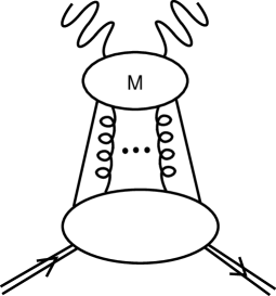
Figure 1: Schematic diagram for Compton scattering in terms of quark and gluon scattering amplitudes and their correlation functions in the nucleon.

The pair of light-cone four-vectors $p^{\mu}=\Lambda(1,0,0,1)/\sqrt{2}$ and $n^{\mu}=(1,0,0,-1)/(\sqrt{2}\Lambda)$ define a collinear basis in which the nucleon and photon momenta are written $P^{\mu}=p^{\mu}+M^{2}n^{\mu}/2$ and $q^{\mu}=-x_{B}p^{\mu}+\nu n^{\nu}$, respectively, where $\Lambda$ is an arbitrary dimensionful parameter. Intermediate quark and gluon momenta can also be expressed in this basis:

$$k_{j}^{\mu}=(k_{j}\cdot n)p^{\mu}+(k_{j}\cdot p)n^{\mu}+k_{j}^{\perp}\ ,$$ (5)

and the full result for $M^{\mu\nu}_{i}$ can be expanded about $k_{j}^{\mu}=(k_{j}\cdot n)p^{\mu}$. The leading term in this expansion can be interpreted as scattering of collinear partons with Feynman momentum fractions $x_{j}=k_{j}\cdot n$. Because the partons are on-shell, $M^{\mu\nu}_{i}$ can be viewed as the parton scattering S-matrix element. In principle, one must multiply by parton wave function renormalization factors to get the proper S-matrix element. However, in dimensional regularization, the absence of a physical scale at the massless poles of the quark and gluon propagators reduces these contributions to unity. Subleading terms in the expansion of $M^{\mu\nu}_{i}$ are parton scattering S-matrix elements with insertions of certain vertices associated with powers of $k_{j}^{\perp}$ and $k^{-}_{j}(\equiv p\cdot k_{j})$. For instance, with one power of quark momentum $k_{j}^{\perp}$, the subleading term is calculated with one insertion of the vector vertex $i\gamma^{\alpha}_{\perp}$ to one of the quark propagators. Because S-matrix elements and their relatives are gauge invariant, one may choose any gauge for the internal gluon propagators in $M^{\mu\nu}_{i}$. We use Feynman’s choice in our calculation.

After the collinear expansion and integration over the quark-gluon four momenta, the convolution of Eq. (4) involves integrating over the parton Feynman variables $x_{j}=(k_{j}\cdot n)$. The correlation functions $\Gamma_{iB}$ are matrix elements of gauge-invariant nonlocal quark and gluon operators in one-to-one correspondence with the external parton states in $M^{\mu\nu}_{i}$. In particular, when $M^{\mu\nu}_{i}$ contains momentum-related vertex insertions, the quark and/or gluon fields in $\Gamma_{iB}$ appear with partial derivatives. The collinear expansion results in all QCD fields separated in spacetime along the light-cone direction $n^{\mu}$. As in the leading-twist case, expanding the gluon polarization indices and summing over all contributions from longitudinally-polarized gluons generates straightline gauge-links which connect fields at separate spacetime points. To simplify the derivation of a factorization formula, we use the light-cone gauge ($A\cdot n=A^{+}=0$), or link-free, expression for $\Gamma_{iB}$. This gauge choice allows one to focus on the physical partons without worrying about the effects of the longitudinally polarized gluons. The gauge-invariant form of the factorization is recovered simply by imposing gauge invariance on the final form of parton correlations.

As we have argued above, $M_{i}^{\mu\nu}$ is ultraviolet finite because the on-shell wave function renormalization is trivial in dimensional regularization. Nevertheless, due to the massless on-shell external states, $M_{i}^{\mu\nu}$ has infrared divergences showing up as $1/\epsilon$ poles. These divergences may be factorized in the perturbative sense

$$M^{\mu\nu}_{i}=C^{\mu\nu}_{i}\otimes P_{i}\ ,$$ (6)

where $C_{i}^{\mu\nu}$ is the finite coefficient function and $P_{i}$ contains only the $1/\epsilon$ poles. On the other hand, the infrared-finite quantities $\Gamma_{iB}$ contain ultraviolet divergences which also show up as $1/\epsilon$ poles. When the infrared poles in $P_{i}$ cancel all the ultraviolet poles in $\Gamma_{iB}$, $T^{\mu\nu}$ is said to be factorizable. The product $P_{i}\Gamma_{iB}$ defines the renormalized parton correlation functions $\Gamma_{i}$. The final factorization formula for the Compton amplitude is then

$$T^{\mu\nu}=\sum_{i}C^{\mu\nu}_{i}\otimes\Gamma_{i}\ ,$$ (7)

where $C^{\mu\nu}_{i}$ is a well-defined perturbation series in $\alpha_{s}$ and $\Gamma_{i}$ is a finite nonperturbative distribution.

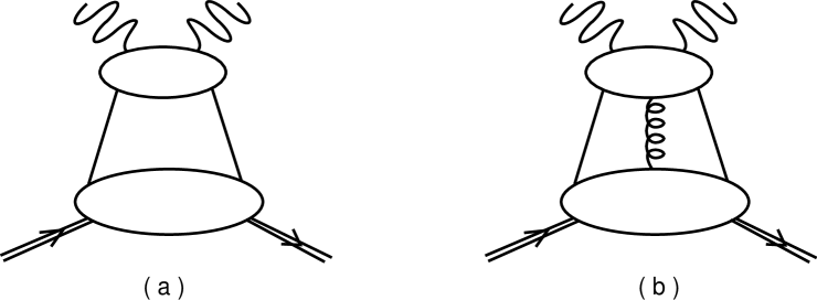
Figure 2: Parton intermediate states appearing in the twist-three Compton amplitude.

We apply the above discussion to Compton scattering on a transversely polarized nucleon. As shown in Fig. 2, the non-singlet twist-three process involves two possible intermediate parton states in the light-cone gauge. First is the two-quark state with the transverse momentum flowing through $M_{qq}^{\mu\nu}$, as shown in Fig. 2a. After Taylor-expansion, we keep only the contribution with exactly one insertion of the $i\gamma^{\alpha}_{\perp}$ vertex. The corresponding correlation function is

$$\Gamma_{qqB}^{\alpha}(x,y) = \int{d\lambda\over 2\pi}{d\mu\over 2\pi}e^{i\lambda x}e^{i\mu(y-x)}\langle PS|\bar{\psi}(0)i\partial^{\alpha}_{\perp}\psi(\lambda n)|PS\rangle$$ (8)

$$= \delta(x-y)\int{d\lambda\over 2\pi}e^{i\lambda x}\langle PS|\bar{\psi}(0)i\partial^{\alpha}_{\perp}\psi(\lambda n)|PS\rangle\ ,$$

where the Dirac and color indices on quark fields are open and $\alpha$ is perpendicular to $p^{\mu}$ and $n^{\mu}$. The second intermediate parton state involves two quark lines and one gluon line, as shown in Fig. 2b. If we use the Feynman rule $it^{a}\gamma^{\alpha}_{\perp}$ for the gluon attachment to $M^{\mu\nu}_{qgq}$, the corresponding correlation function is

$$\Gamma_{qgqB}^{\alpha}(x,y)=\int{d\lambda\over 2\pi}{d\mu\over 2\pi}e^{i\lambda x}e^{i\mu(y-x)}\langle PS|\bar{\psi}(0)(-g_{B})A^{\alpha}_{\perp}(\mu n)\psi(\lambda n)|PS\rangle\ .$$ (9)

We remind the reader that all fields and the couplings here are bare. To decouple the spin and color indices in $M^{\mu\nu}_{i}$ and $\Gamma_{iB}$, we write explicitly

$$\Gamma_{qqB}^{\alpha ij}(x,y) = \left(S_{\perp}^{\alpha}\gamma_{5}\not\!p\Gamma_{1(qq)B}(x,y)+iT^{\alpha}_{\perp}\not\!p\Gamma_{2(qq)B}(x,y)\right){\delta_{ij}\over N_{c}}\ ,$$

$$\Gamma_{qgqB}^{\alpha ija}(x,y) = \left(S_{\perp}^{\alpha}\gamma_{5}\not\!p\Gamma_{1(qgq)B}(x,y)+iT^{\alpha}_{\perp}\not\!p\Gamma_{2(qgq)B}(x,y)\right){t^{a}_{ij}\over N_{c}C_{F}}\ ,$$ (10)

where $N_{c}$ is the number of colors, $C_{F}=(N_{c}^{2}-1)/(2N_{c})$, and $T^{\alpha}=\epsilon^{\alpha\beta\gamma\delta}S_{\perp\beta}p_{\gamma}n_{\delta}$. In dimensional regularization, $\gamma_{5}$ must be defined explicitly. Here, we follow t’ Hooft and Veltman’s convention.

With appropriate insertions of light-cone gauge links, which can be generated by summing over intermediate states with additional longitudinally-polarized gluons, we define the following gauge-invariant parton correlations et ; ji :

$$K_{iB}(x,y)=\Gamma_{i(qq)B}(x,y)+\Gamma_{i(qgq)B}(x,y)\ .$$ (11)

One may argue that this is not the only way to obtain gauge invariant correlations. In particular, the combination $(y-x)\Gamma^{\alpha}_{i(qgq)B}(x,y)$ is the light-cone expression for a gauge invariant distribution involving the gluon field strength rather than the covariant derivative. On the other hand, these contributions necessarily involve coefficients $C_{i(qgq)\alpha}^{\mu\nu}(x,y)$ that vanish when $x=y$. Eq.(8) then implies that one can consider instead the combination of Eq.(11) free of charge. Hence these are the only distributions relevant to our process. Using hermitian conjugation, it is easy to show that $K_{1B}$ is symmetric in $x$ and $y$ and $K_{2B}$ is antisymmetric. We will use these symmetries to simplify our presentation of the coefficient functions.

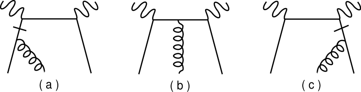
Figure 3: Tree contribution to $M^{\mu\nu}_{qgq}$. The contribution to $M^{\mu\nu}_{qq}$ is obtained by replacing the gluon vertex by $i\gamma^{\alpha}_{\perp}$.

Let us consider the use of the above approach to the tree diagrams shown in Fig. 3, where we have shown $M_{gqg}^{\mu\nu}$ only. Those diagrams for $M_{qq}^{\mu\nu}$ can be obtained simply by replacing the gluon interaction $it^{a}\gamma^{\alpha}_{\perp}$ by the transverse vector vertex $i\gamma^{\alpha}_{\perp}$. Figure 3 corresponds to the following on-shell process: a quark and gluon with four-momenta $xp^{\mu}$ and $(y-x)p^{\mu}$, respectively, scatter with a photon of four-momentum $q^{\mu}$, producing a quark of four-momentum $yp^{\mu}$ and a forward photon. The Compton amplitude can easily be calculated using the usual Feynman rules. When the quark and gluon combine before or after interacting with the photons, the intermediate propagator, $i/(y\not\!p)$, drawn with a bar in Fig. 3, is singular and needs regularization. Adding an infinitesimal $\lambda\not\!n$, one arrives at

$${i(y\not\!p+\lambda\not\!n)\over(yp+\lambda n)^{2}}={i\not\!p\over 2\lambda}+{i\not\!n\over 2y}\ .$$ (12)

The first term yields zero when acting on the external quark wave function, so only the second term contributes. Combining the result from $M_{qq}^{\mu\nu}$ and taking into account crossing symmetry, we find the following gauge-invariant expression for the tree-level Compton amplitude

$$T^{\mu\nu} =-i\epsilon^{\mu\nu\alpha\beta}q_{\alpha}S_{\perp\beta}{1\over\nu}\int dxdy\sum_{i}\hat{e}^{2}_{i}$$ (13)

$$\times\;{2\over x(x_{B}-x)}\left[K_{1i}(x,y)+K_{2i}(x,y)\right]-(x_{B}\rightarrow-x_{B})\ ,$$

where $\hat{e}^{2}_{i}=e^{2}_{i}-\bar{e}^{2}$ is the non-singlet part of the quark charge squared and $\bar{e}^{2}=\sum_{i}e_{i}^{2}/n_{f}$. The integration has support only for $\{x,y\}\in[-1,1]$. When $|x_{B}|<1$, the above expression develops an imaginary part through $x_{B}\rightarrow x_{B}-i\epsilon$. Using the optical theorem, one obtains the following tree result for $g^{NS}_{T}$,

$$g_{T}^{NS(0)}(x_{B},Q^{2})={1\over 2}\sum_{i}\hat{e}_{i}^{2}{2\over x_{B}}\int^{1}_{-1}dy\left(K_{1i}(x_{B},y)+K_{2i}(x_{B},y)\right)+(x_{B}\rightarrow-x_{B})\ .$$ (14)

¿From QCD equations of motion, one can show

$$\Delta q_{T}(x)={2\over x}\int^{1}_{-1}dy\left(K_{1}(x,y)+K_{2}(x,y)\right)\ ,$$ (15)

where $\Delta q_{T}(x)$ is defined as

$$\Delta q_{T}(x)={1\over 2}\int{d\lambda\over 2\pi}e^{i\lambda x}\langle PS_{\perp}|\bar{\psi}(x)\gamma_{\perp}\gamma_{5}\psi(0)|PS_{\perp}\rangle\ .$$ (16)

This object seems to have a simple physical interpretation.

The tree level result suggests the following all-order factorization formula for the non-singlet part of $g_{T}$,

$$g^{NS}_{T}(x_{B},Q^{2}) = \sum_{i}\hat{e}_{i}^{2}\int^{1}_{-1}{dxdy\over xy}\left(C_{1}\left({x_{B}\over x},{x_{B}\over y},\alpha_{s}\right)K_{1i}(x,y)\right.$$ (17)

$$\left.+C_{2}\left({x_{B}\over x},{x_{B}\over y},\alpha_{s}\right)K_{2i}(x,y)\right)+(x_{B}\rightarrow-x_{B})\ .$$

$C_{1,2}$ can be written in terms of a perturbation series in the strong coupling $\alpha_{s}$,

$$C_{1,2}=\sum_{i}C_{1,2}^{(i)}\left({\alpha_{s}\over 2\pi}\right)^{i}\ .$$ (18)

The tree result yields

$$C_{1,2}^{(0)}\left({x_{B}\over x},{x_{B}\over y}\right)=y\delta(x-x_{B})\;\;.$$ (19)

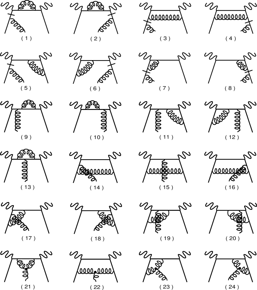
Figure 4: One-loop contribution to $M^{\mu\nu}_{qgq}$. The contribution to $M^{\mu\nu}_{qq}$ is obtained by modifying the external gluon vertex in the first 20 diagrams.

Now we come to the main subject of the paper: one-loop radiative corrections for $g^{NS}_{T}(x_{B},Q^{2})$. All the Feynman diagrams for $M_{qgq}^{\mu\nu}$ are shown in Fig. 4. The first 12 diagrams have color factor $C_{F}$, the next 8 come with the factor $C_{F}-C_{A}/2$, and the final 4 with $C_{A}=N_{c}$. Since the external transverse momentum of the quark only goes through the quark propagators, the Taylor-expansion of $M_{qq}^{\mu\nu}$ yields the vector vertex insertion on the quark line only. These diagrams correspond to the first 20 diagrams in Fig. 4 with the external gluon vertex replaced by the vector vertex. An inspection of the one-loop Feynman integrals reveals a simple rule: $M_{qq}^{\mu\nu}$ is just the $C_{F}$ part of $M_{qgq}^{\mu\nu}$ and, hence, the former need not be calculated separately.

Since all Feynman diagrams are computed in bare perturbation theory, the result depends on the bare coupling $g_{B}$. We replace it with a renormalized coupling in the $\overline{\rm MS}$ scheme, with a difference of higher order in $\alpha_{s}(\mu^{2})$. After a lengthy calculation involving one-loop integrals with up to five internal Feynman propagators, we find

$$S_{T}^{(1)NS}(x_{B},Q^{2}) = \sum_{i}\hat{e}_{i}^{2}\int{dxdy\over xy}\left[M^{(1)}_{1}\left({x\over x_{B}},{y\over x_{B}}\right)K_{1iB}(x,y)\right.$$ (20)

$$\left.+M^{(1)}_{2}\left({x\over x_{B}},{y\over x_{B}}\right)K_{2iB}(x,y)\right]-(x_{B}\rightarrow-x_{B})\ .$$

Explicit expressions for the $M$’s in the region $|x_{B}|>1$ can be found in the Appendix.

Now we are ready to show that $S^{NS}_{T}(x_{B},Q^{2})$ is factorizable at the one-loop level, i.e., the infrared poles $1/\epsilon$ in $M^{(1)}_{i}$ match the ultraviolet poles in $K_{iB}$. To this end, we use the infrared poles in $M_{i}$ to generate a scale evolution equation for the parton distributions. From the result in the Appendix, we find

$${d\over d\ln\mu^{2}}\int^{1}_{-1} dxdy \left({2\over x(x_{B}-x)}\right)(K_{1}(x,y,\mu^{2})+K_{2}(x,y,\mu^{2}))$$ (21)

$$= -{\alpha_{s}(\mu^{2})\over 2\pi}\int^{1}_{-1}dxdy\left\{C_{F}K_{1}(x,y,\mu^{2})\left[{-1\over x(x_{B}-x)}+{2\over x^{2}}-{2\over xy}\right.\right.$$

$$-2\left({2x_{B}\over x^{2}y}+{1\over x^{2}}-{x_{B}\over x^{3}}+{2\over x(x_{B}-x)}\right)\log\left({x_{B}-x\over x_{B}}\right)$$

$$\left.+{2\over y-x}\left({2x_{B}\over x(y-x)}+{1\over x_{B}-y}\right)\log\left({x_{B}-y+x\over x_{B}}\right)\right]$$

$$+C_{F}K_{2}(x,y,\mu^{2})\left[{-1\over x(x_{B}-x)}+{2\over x^{2}}-2\left({1\over x^{2}}-{x_{B}\over x^{3}}+{2\over x(x_{B}-x)}\right)\right.$$

$$\left.\times\log\left({x_{B}-x\over x_{B}}\right)-{2\over(y-x)(x_{B}-y)}\log\left({x_{B}-y+x\over x_{B}}\right)\right]$$

$$+{C_{A}\over 2}K_{1}(x,y,\mu^{2})\left[-{4x_{B}\over xy(y-x)}\log\left({x_{B}-x\over x_{B}}\right)\right.$$

$$\left.-{2x_{B}\over y-x}\left({2\over x(y-x)}+{1\over x_{B}-y}\right)\log\left({x_{B}-y+x\over x_{B}}\right)\right]$$

$$\left.+{C_{A}\over 2}K_{2}(x,y,\mu^{2}){2\over(y-x)(x_{B}-y)}\log\left({x_{B}-y+x\over x_{B}}\right)\right\}\ .$$

Expanding the above in the large $x_{B}$ limit, we get the evolution equation for the moments of the parton distributions. A detailed check shows that the equation is identical to that in Ref. bkl obtained by studying the ultraviolet divergences present in the twist-three operators. In particular, in the large $N_{c}$ limit, the above equation becomes autonomous ali ; osborne .

The final step of the calculation is to take the imaginary part of the factorized $S^{NS}_{T}(x_{B},Q^{2})$ to get a factorized expression for the structure function $g^{NS}_{T}(x_{B},Q^{2})$ in the physical region $x_{B}<1$. With the definition in Eq. (19) we find the following result for the coefficient functions,

$$C_{1}^{(1)}\left({x_{B}\over x},{x_{B}\over y}\right) =C_{F}y\left\{-2\delta(x-x_{B})+\theta\left({x\over x_{B}}-1\right)\left[{3/2\over(x_{B}-x)_{+}}-{x_{B}\over x^{2}}+{6x_{B}\over xy}\right.\right.$$ (22)

$$+{2x_{B}\over y(y-x)}-{1/2\over x}-{1\over y}-{1\over y-x}-\left({2x_{B}\over xy}+{1\over x}-{x_{B}\over x^{2}}\right)\log\left({x-x_{B}\over x_{B}}\right)$$

$$\left.-\left({2\over(x_{B}-x)}\log\left({x-x_{B}\over x_{B}}\right)\right)_{+}\right]$$

$$+\theta\left({y-x\over x_{B}}-1\right){1\over y-x}\left[1-{2x\over x_{B}-y}-{4x_{B}\over y-x}\right.$$

$$\left.+\left({2x_{B}\over y-x}+{x\over x_{B}-y}\right)\log{\left(y-x-x_{B}\over x_{B}\right)}\right]$$

$$+\delta(x-x_{B})\log{\left(1-x_{B}\over x_{B}\right)}\left[-{3\over 2}+\log{\left(1-x_{B}\over x_{B}\right)}\right]$$

$$\left.+\delta(y-x_{B}){2x\over x_{B}-x}\log\left({x\over x_{B}}\right)\left[1-{1\over 4}\log\left({x\over x_{B}}\right)\right]\right\}$$

$$+{C_{A}\over 2}y\left\{\theta\left({x\over x_{B}}-1\right){x_{B}\over y}\left[{1\over x_{B}-y}+{4\over y-x}\left(1-{1\over 2}\log\left({x_{B}-x\over x_{B}}\right)\right)\right]\right.$$

$$-\theta\left({y-x\over x_{B}}-1\right){1\over(y-x)}\left[1-\left({2x\over x_{B}-y}+{4x_{B}\over(y-x)}\right)\right.$$

$$\left.\times\left(1-{1\over 2}\log\left({y-x-x_{B}\over x_{B}}\right)\right)\right]-\delta(y-x_{B})\left[\log\left({x-x_{B}\over x_{B}}\right)\right.$$

$$\left.\left.+{2x\over(x_{B}-x)}\left(1-{1\over 4}\log\left({x\over x_{B}}\right)\right)\log\left({x\over x_{B}}\right)\right]\right\}\ ,$$

$$C_{2}^{(1)}\left({x_{B}\over x},{x_{B}\over y}\right) =C_{F}y\left\{-2\delta(x-x_{B})+\theta\left({x\over x_{B}}-1\right)\left[{3/2\over(x_{B}-x)_{+}}-{x_{B}\over x^{2}}\right.\right.$$ (23)

$$-{1/2\over x}+{1\over y}\left.-\left({1\over x}-{x_{B}\over x^{2}}\right)\log\left({x-x_{B}\over x_{B}}\right)-\left({2\over(x_{B}-x)}\log\left({x-x_{B}\over x_{B}}\right)\right)_{+}\right]$$

$$+\theta\left({y-x\over x_{B}}-1\right){1\over y-x}\left[1+{2x\over x_{B}-y}-{x\over x_{B}-y}\log{\left(y-x-x_{B}\over x_{B}\right)}\right]$$

$$+\delta(x-x_{B})\log{\left(1-x_{B}\over x_{B}\right)}\left[-{3\over 2}+\log{\left(1-x_{B}\over x_{B}\right)}\right]$$

$$\left.-\delta(y-x_{B}){2x\over x_{B}-x}\log\left({x\over x_{B}}\right)\left[1-{1\over 4}\log\left({x\over x_{B}}\right)\right]\right\}$$

$$+{C_{A}\over 2}y\left\{-{x_{B}\over y(x_{B}-y)}\theta\left({x\over x_{B}}-1\right)\right.$$

$$-{1\over y-x}\left[1+{2x\over x_{B}-y}\left(1-{1\over 2}\log\left({y-x-x_{B}\over x_{B}}\right)\right)\right]\theta\left({y-x\over x_{B}}-1\right)$$

$$\left.+\delta(y-x_{B})\left[\log\left({x-x_{B}\over x_{B}}\right)+{2x\over x_{B}-x}\left(1-{1\over 4}\log\left({x\over x_{B}}\right)\right)\log\left({x\over x_{B}}\right)\right]\right\}$$

The definition of the + functions can be found in Ref. dglap . The support for the parton correlations limits $y-x$ to the interval $[-1,1]$.

To check the Burkhardt-Cottingham sum rule bc , we integrate $g^{NS}_{T}(x_{B},Q^{2})$ over $x_{B}$. Assuming the integration over $x$ and $y$ can be interchanged with that of $x_{B}$, one obtains

$$\int^{1}_{0}dx_{B}g^{NS}_{T}(x_{B},Q^{2})={1\over 2}\sum_{i}\hat{e}_{i}^{2}\left(1-{7\over 2}C_{F}{\alpha_{s}\over 2\pi}\right)\langle PS|\overline{\psi}_{i}\gamma_{\perp}\gamma_{5}\psi_{i}|PS\rangle\ .$$ (24)

Here the coefficient $7/2$ reduces to $3/2$ if we define $\gamma_{5}$ so that the non-singlet axial current is conserved. Compared with the factorization formula for $g_{1}(x_{B},Q^{2})$, we have the Burkhardt-Cottingham sum rule at one loop

$$\int^{1}_{0}dx_{B}g^{NS}_{2}(x_{B},Q^{2})=0\ .$$ (25)

If the order of integration cannot be interchanged because of the singular behevior of the parton distributions at small $x$ and $y$, the above sum rule may be violated. Indeed some small $x_{B}$ study does indicate such singular behavior smallx .

Finally, we consider the next-to-leading order correction to the non-singlet part of the $x^{2}$ moment of $g_{T}(x_{B},Q^{2})$. In the leading order, it is well known :

$$\int^{1}_{0}dx~{}x^{2}g^{NS}_{T}(x,Q^{2})={1\over 3}\sum_{i}\hat{e}_{i}^{2}\left({1\over 2}a_{2i}(Q^{2})+d_{2i}(Q^{2})\right)\ ,$$ (26)

where $a_{2}$ is the second moment of the $g_{1}(x,Q^{2})$ structure function and $d_{2}$ is a twist-three matrix element jj . Using the coefficient functions found above, we see that

$$\int^{1}_{0}dxx^{2}g^{NS}_{T}(x,Q^{2}) = {1\over 3}\sum_{i}\hat{e}_{i}^{2}\left\{{a_{2i}\over 2}\left[1+{\alpha_{s}(Q^{2})\over 4\pi}{7\over 12}C_{F}\right]\right.$$ (27)

$$\phantom{{1\over 3}\sum_{i}\hat{e}_{i}^{2}}\quad\left.+d_{2i}\left[1+{\alpha_{s}(Q^{2})\over 4\pi}\left({27\over 4}C_{A}-{29\over 3}C_{F}\right)\right]\right\}\ .$$

Using the next-to-leading result for $g_{1}(x,Q^{2})$kodaira , we find

$$\int^{1}_{0}dxx^{2}\left(g^{NS}_{T}(x,Q^{2})-{1\over 3}g^{NS}_{1}(x,Q^{2})\right)={1\over 3}\sum_{i}\hat{e}_{i}^{2}d_{2i}\left(1+{\alpha_{s}(Q^{2})\over 4\pi}\left({27\over 4}C_{A}-{29\over 3}C_{F}\right)\right)\ .$$ (28)

Notice that the combination of $g_{T}$ and $g_{1}$ relevant to $d_{2}$ receives no radiative correction.

To summarize, we have extended the leading-twist factorization formalism to higher twist. The extension mainly involves a correct identification of the intermediate parton states and arranging different calculations into gauge invariant combinations. Because of the multipartons in the initial state, higher-twist perturbative calculations are, in general, much more complicated than the leading twist cases. As an example, we have presented the one-loop coefficient functions the twist-three process involving forward Compton scattering on a transversely polarized nucleon target. This result can be combined with a two-loop calculation of the twist-three evolution equation to yield a next-to-leading order formalism for the $g_{2}$ structure function.

Appendix

In this appendix, we present the tree and one-loop Compton amplitudes for virtual photon scattering on a transversely polarized nucleon in the unfactorized form. To simplify the expressions, we assume $|x_{B}|>1$ so that the amplitudes are purely real. With $\epsilon^{0123}=+1$, we write the Compton tensor as

$$T^{\mu\nu}=-i\epsilon^{\mu\nu\alpha\beta}q_{\alpha}S_{\perp\beta}{1\over\nu}S_{T}(x_{B},Q^{2})\ .$$ (29)

In QCD, we can write,

$$S^{NS}_{T}(x_{B},Q^{2}) = \sum_{i}\hat{e}_{i}^{2}\int^{1}_{-1}{dxdy\over xy}\left[M_{1}\left({x\over x_{B}},{y\over x_{B}}\right)K_{1iB}(x,y)\right.$$ (30)

$$\left.+M_{2}\left({x\over x_{B}},{y\over x_{B}}\right)K_{2iB}(x,y)\right]-(x_{B}\rightarrow-x_{B})\ ,$$

where the $K$’s are unrenormalized parton distributions as defined in the text, $M$’s are perturbation series in $\alpha_{s}$ and have infrared poles.

At tree level, the result is well known,

$$M^{(0)}_{1}(x,y)=M^{(0)}_{2}(x,y)={2y\over 1-x}\ .$$ (31)

At the one-loop level, the following amplitudes are associated with distributions with a covariant derivative,

$$M^{(1)}_{1}(x,y) = {\alpha_{sB}\over 2\pi}C_{F}\left({\bar{\mu}^{2}\over Q^{2}}\right)^{\epsilon/2}\left\{{2\over\epsilon}\left[{-y\over(1-x)}+{2y\over x}-2-2\left({2\over x}+{y\over x}-{y\over x^{2}}+{2y\over 1-x}\right)\right.\right.$$ (32)

$$\left.\times\log(1-x)+{2y\over y-x}\left({2\over y-x}+{x\over 1-y}\right)\log(1-y+x)\right]$$

$$-2\left({2y\over 1-x}-{y\over x}+3\right)-\left({3y\over 1-x}-{2y\over x^{2}}\right.$$

$$+\left.{12\over x}+{4\over y-x}-{y\over x}-2-{2y\over y-x}\right)\log(1-x)$$

$$-{2y\over y-x}\left(1-{2x\over 1-y}-{4\over y-x}\right)\log(1-y+x)$$

$$+\left({2\over x}+{y\over x}-{y\over x^{2}}+{2y\over 1-x}\right)\log^{2}(1-x)$$

$$\left.-{y\over y-x}\left({2\over y-x}+{x\over 1-y}\right)\log^{2}(1-y+x)\right\}$$

$$+{\alpha_{sB}\over 2\pi}{C_{A}\over 2}\left({\bar{\mu}^{2}\over Q^{2}}\right)^{\epsilon/2}\left\{{2\over\epsilon}\left[-{4\over y-x}\log(1-x)\right.\right.$$

$$\left.-{2y\over y-x}\left({2\over y-x}+{x\over 1-y}\right)\log(1-y+x)\right]$$

$$-2\left({1\over 1-y}+{4\over y-x}\right)\log(1-x)$$

$$+{2y\over y-x}\left(1-{2x\over 1-y}-{4\over y-x}\right)\log(1-y+x)$$

$$+{2\over y-x}\log^{2}(1-x)$$

$$\left.+{y\over y-x}\left({2\over y-x}+{x\over 1-y}\right)\log^{2}(1-y+x)\right\}\ ,$$

$$M^{(1)}_{2}(x,y) = {\alpha_{sB}\over 2\pi}C_{F}\left({\bar{\mu}^{2}\over Q^{2}}\right)^{\epsilon/2}\left\{{2\over\epsilon}\left[{-y\over(1-x)}+{2y\over x}-2\left({y\over x}-{y\over x^{2}}+{2y\over 1-x}\right)\right.\right.$$ (33)

$$\left.\times\log(1-x)-{2xy\over(y-x)(1-y)}\log(1-y+x)\right]$$

$$-2\left({2y\over 1-x}-{y\over x}\right)-\left({3y\over 1-x}-{2y\over x^{2}}-{y\over x}+2\right)\log(1-x)$$

$$-{2y\over y-x}\left(1+{2x\over 1-y}\right)\log(1-y+x)$$

$$+\left({y\over x}-{y\over x^{2}}+{2y\over 1-x}\right)\log^{2}(1-x)$$

$$\left.+{xy\over(y-x)(1-y)}\log^{2}(1-y+x)\right\}$$

$$+{\alpha_{sB}\over 2\pi}{C_{A}\over 2}\left({\bar{\mu}^{2}\over Q^{2}}\right)^{\epsilon/2}\left\{{2\over\epsilon}{2xy\over(y-x)(1-y)}\log(1-y+x)\right.$$

$$+{2\over 1-y}\log(1-x)$$

$$+{2y\over y-x}\left(1+{2x\over 1-y}\right)\log(1-y+x)$$

$$\left.-{xy\over(y-x)(1-y)}\log^{2}(1-y+x)\right\}\ ,$$

where $\epsilon=4-d$, $\bar{\mu}^{2}=4\pi e^{-\gamma_{E}}\mu^{2}$, and $\gamma_{E}$ is the Euler constant.

References

(1)
A. Mueller, Perturbative Quantum Chromodynamics (World
Scientific, Singapore, 1989).
(2)
V. N. Gribov and L. N. Lipatov, Sov. J. Nucl. Phys. 15, 78 (1972);
G. Altarelli and G. Parisi, Nucl. Phys. B 126, 298 (1977);
Y. L. Dokshitser, Sov. Phys.-JETP 46, 641 (1977).
(3)
J. Qiu and G. Sterman, Nucl. Phys. B 353, 137 (1991).
(4)
P. Bosted for E155x Collaboration, Nucl. Phys. A 666-667, 300 (2000).
(5)
JLab workshop on 12 GeV upgrade, January, 2000.
(6)
A. J. G. Hey and J. E. Mandula, Phys. Rev. D 5, 2610 (1972);
M. A. Ahmed and G. G. Ross, Nucl. Phys. B 111, 441 (1976);
K. Sasaki, Prog. Theor. Phys. 54, 1816 (1975).
(7)
J. Kodaira, S. Matsuda, K. Sasaki, T. Uematsu, Nucl. Phys. B
159, 99 (1979).
(8)
R. Mertig and W. L. van Neervan, Z. Phys. C 60, 489 (1993);
G. Altarelli, B. Lampe, P. Nason and G. Ridolfi,
Phys. Lett. B 334, 187 (1994);
J. Kodaira, S. Matsuda, T. Uematsu, and K. Sasaki,
Phys. Lett. B 345, 527 (1995);
P. Mathews, V. Ravindran, and K. Sridhar,
hep-ph/9607385;
A. Gabieli, G. Ridolfi Phys, Lett. B 417, 369 (1998).
(9)
E. V. Shuryak and A. I. Vainshtein, Nucl. Phys. B199,
951 (1982).
(10)
A. P. Bukhvostov, E. A. Kuraev, and L. N. Lipatov,
JETP Lett. 37, 484 (1983);
Sov. Phys. JETP 60, 22 (1984).
(11)
P. G. Ratcliffe, Nucl. Phys. B 264, 493 (1989);
I. I. Balitsky and V. M. Braun, Nucl. Phys. B 311, 541
(1989);
X. Ji and C. Chou, Phys. Rev. D 42, 3637 (1990);
B. Geyer, D. Müller and D. Robaschik, hep-ph/9611452;
J. Kodaira, Y. Yasui, K. Tanaka and T. Uematsu, Phys. Lett. B387, 855 (1996).
(12)
A. V. Efremov and O. V. Teryaev, Sov. J. Nucl. Phys. 36, 140 (1982).
(13)
R. L. Jaffe and X. Ji, Phys. Rev. D 43, 724 (1991).
(14)
X. Ji, Nucl. Phys. B 402, 217 (1993).
(15)
G. Curci, W. Furmanski, and R. Petronzio, Nucl. Phys. B 175, 27 (1980).
(16)
J. Qiu and G. Sterman, Phys. Rev. Lett. 67, 2264 (1991);
Phys. Rev. D 59, 014004 (1999).
(17)
A. Ali, V. M. Braun and G. Hiller, Phys. Lett.
B 266, 117 (1991).
(18)
X. Ji and J. Osborne, Eur. Phys. J. C 9, 487 (1999).
(19)
H. Burkhardt and W. N. Cottingham, Ann. Phys. (N. Y.) 56, 453 (1970).
(20)
I. P. Ivanov, N. N. Nikolaev, A. V. Pronyaev, W. Schafer,
Phys. Lett. B 457, 218 (1999).