SLAC-PUB-8469 June 2000

The $g-2$ of the Muon in Localized Gravity Models

H. Davoudiasl, J.L. Hewett, and T.G. Rizzo

Stanford Linear Accelerator Center

Stanford University

Stanford CA 94309, USA

The $(g-2)$ of the muon is well known to be an important model building constraint on theories beyond the Standard Model. In this paper, we examine the contributions to $(g-2)_{\mu}$ arising in the Randall-Sundrum model of localized gravity for the case where the Standard Model gauge fields and fermions are both in the bulk. Using the current experimental world average measurement for $(g-2)_{\mu}$, we find that strong constraints can be placed on the mass of the lightest gauge Kaluza-Klein excitation for a narrow part of the allowed range of the assumed universal 5-dimensional fermion mass parameter, $\nu$. However, employing both perturbativity and fine-tuning constraints we find that we can further restrict the allowed range of the parameter $\nu$ to only one fourth of its previous size. The scenario with the SM in the RS bulk is thus tightly constrained, being viable for only a small region of the parameter space.

The existence of extra spacetime dimensions has recently been suggested[1, 2, 3] as a means to explain the hierarchy. In one scenario of this kind from Arkani-Hamed, Dimopoulos, and Dvali (ADD)[1], the apparent hierarchy is generated by a large volume for the extra dimensions. In this case, the fundamental Planck scale in $4+n$-dimensions, $M$, can be reduced to the TeV scale and is related to the observed 4-d Planck scale, $\overline{M}_{Pl}$, through the volume $V_{n}$ of the compactified dimensions, $\overline{M}_{Pl}^{2}=V_{n}M^{2+n}$. In a second scenario due to Randall and Sundrum (RS)[2], the observed hierarchy is induced through an exponential warp factor which arises from a non-factorizable geometry. An exciting feature of these approaches is that they both lead to concrete and distinctive phenomenological tests[4, 5] at the TeV scale.

In addition to collider tests, loop-order processes, such as rare transitions which are suppressed in the Standard Model (SM) or radiative corrections to perturbatively calculable processes, can provide complementary information about new physics. One such traditional quantity is the $(g-2)$ of the $\mu$[6]. Currently the SM prediction is approximately $1\sigma$ higher than that of the World Average measured value, with the difference between the theoretical and experimental results being $a^{exp}_{\mu}-a^{SM}_{\mu}=(43\pm 45)\times 10^{-10}$, where $a=(g-2)/2$. This corresponds to a $95\%$ CL upper bound on the magnitude of a new negative contribution, $\Delta a_{\mu}$, of $-3.1\times 10^{-9}$. The E821 experiment at BNL is expected to reduce the experimental error on $a_{\mu}^{exp}$ by approximately an order of magnitude during the next few years to the level of 0.35ppm which is below the current SM theory error of 0.60ppm. The SM error will also decrease in the future as more data on the $R$ ratio in the low energy region becomes available. The size of the contribution to $(g-2)_{\mu}$ in the ADD scenario has been calculated in Ref.[7] and results in interesting constraints. In this paper, we examine this quantity within the RS model in the case where the SM fields propagate in the bulk with the expectation from our earlier work[8] that existing data will yield interesting bounds over a region of the parameter space. With an anticipated ten-fold increase in the experimental precision in the not too distant future, these bounds should soon improve if no signal for new physics is observed.

In its original construction, the RS model consists of two 3-branes each being stabilized[9] at an $S^{1}/Z_{2}$ orbifold fixed point with a separation of $\pi r_{c}$ between the branes in an additional dimension denoted as $r_{c}\phi$. The model initially postulated that only gravity was allowed to propagate in the higher dimensional anti-deSitter bulk with the SM fields being confined to one of the 3-branes. The exponential ‘warp’ factor $e^{-kr_{c}\phi}$, with $k$ being a 5-d space-time curvature parameter of order the Planck scale, is responsible for generating the observed hierarchy assuming the scale of physics on the SM brane located at $\phi=\pi$ is $\Lambda_{\pi}=\overline{M}_{Pl}e^{-kr_{c}\pi}\simeq 1$ TeV with $kr_{c}\sim 11-12$. The usual 4-d Planck scale and that of the original 5-d theory are found to be related via $\overline{M}_{Pl}^{2}=M_{5}^{3}/k$. Recently, a series of authors[8, 10] have considered peeling the SM gauge and matter fields off of the wall in the limit where their back-reaction on the RS metric can be ignored. (There are a number of arguments which strongly suggest that if the Higgs is the source of electroweak symmetry breaking it must remain on the wall[8, 10].) It is the existence of these SM bulk fields that allows for a potentially sizeable contribution to $(g-2)_{\mu}$. In what follows we use the notation as defined in the last paper listed in Ref.[8].

When the SM gauge and matter fields are allowed to propagate in the bulk, there are three parameters that need to be specified to determine the phenomenological predictions of the RS model: $c\equiv k/\overline{M}_{Pl}$ which is expected to lie in the range 0.01 to 1, the common dimensionless bulk mass parameter for the fermions $\nu\equiv m/k$, where $m$ represents the 5-d fermion mass, which is expected to be of order unity, and the mass of the lightest gauge, fermion or graviton Kaluza-Klein(KK) excitation. We remind the reader that a common value of $\nu$ for all fermions is not a necessary assumption but is certainly the simplest choice and the one which naturally avoids constraints associated with flavor changing neutral currents. For a fixed value of $\nu$,the entire KK spectrum is determined for all fields once the mass of a single KK excitation is known. We recall that the KK spectrums for gravitons, fermions, and gauge bosons are related[8] by the roots of various Bessel functions and that all gauge bosons, i.e., gluons, $W$’s, $Z$’s and $\gamma$’s, have essentially the same excitation spectra.

Note that the limits we obtain below are derived under the assumption that no other new physics is present beyond what is considered here. As with all bounds obtained via indirect means, the presence of additional new interactions may cancel the loop effects and erase or ease the constraints.

Consider the situation where we have two fermions in the bulk, $D$ and $S$, which have the quantum numbers of an $SU(2)_{L}$ doublet and singlet with weak hypercharges $Y=-1/2$ and $-1$, respectively. Following the notation of our previous work, their interactions with the gauge fields can be described by the action,

$$S_{fV}=\int d^{4}x\int r_{c}~{}d\phi\sqrt{G}\left[V^{M}_{n}\left({i\over{2}}\overline{S}\,\gamma^{n}\,{\cal D}_{M}S+h.c.\right)-sgn(\phi)m_{S}\overline{S}S+(S\rightarrow D\right)],$$ (1)

where, $G$ is the determinant of the metric tensor, $V$ is the vielbein, ${\cal D}_{M}$ is a covariant derivative and $h.c.$ denotes the Hermitian conjugate term. Here, as discussed above, we will assume that $m_{D}=m_{S}=k\nu$. Note that gauge interactions do not mix the $D$ and $S$ fields. The $D$ and $S$ fields also interact with the Higgs isodoublet field(s), $H^{0}$, which reside on the wall, i.e.,

$$S_{fH}={\lambda\over{k}}\int d^{4}x\int d\phi\sqrt{G}\ \overline{S}DH^{0}\ \delta(\phi-\pi)+h.c.,$$ (2)

with $\lambda$ being a dimensionless Yukawa coupling. Due to the KK mechanism the fields $D_{L,R}^{(n)}$ and $S_{L,R}^{(n)}$ form separate 4-d towers of Dirac fermions which are degenerate level by level. The KK expansion can be written as $D=\sum D_{L}^{(n)}(x)\chi^{(n)}(\phi)+D_{R}^{(n)}(x)\tau^{(n)}(\phi)$ and $S=\sum S_{L}^{(n)}(x)\tau^{(n)}(\phi)+S_{R}^{(n)}(x)\chi^{(n)}(\phi)$ where the $\nu$-dependent $\chi(\tau)$ fields are $Z_{2}$ even(odd) and are given explicitly in our previous paper. Note that the $Z_{2}$ orbifold symmetry allows couplings of the type $\overline{D_{L}}^{(n)}S_{R}^{(m)}+h.c.$ but not ones of the form $\overline{D_{R}}^{(n)}S_{L}^{(m)}+h.c.$ since the $Z_{2}$ odd wavefunctions vanish on both of the boundaries. After shifting the Higgs field $H^{0}\rightarrow e^{kr_{c}\pi}H$ so that it is canonically normalized, the value of $\lambda$ is fixed as a function of $\nu$ by the requirement that the coupling of the $D_{L}$ and $S_{R}$ zero modes obtains a mass, $m_{\mu}$, once the Higgs gets a vev, $v_{4}=v_{SM}/\sqrt{2}$ with $v_{SM}\simeq 246$ GeV. (It is thus important to observe that in a theory with a fixed value of $\nu$ the set of Yukawa couplings $\lambda_{f}$ associated with the set of SM fermions is clearly hierarchical.) This then fixes the couplings between a Higgs, a zero mode fermion and any tower member to be $C_{0i}^{ffH}=(-1)^{i}~{}{m_{\mu}\over{v_{4}}}\sqrt{F}$, as well as the coupling between two different tower members and the Higgs as $C_{ij}^{ffH}=(-1)^{i+j}~{}{m_{\mu}\over{v_{4}}}F$ (up to a possible $\nu$-dependent sign where),

$$F=2\Big{|}{1-\epsilon^{2\nu+1}\over{1+2\nu}}\Big{|},$$ (3)

with $\epsilon=e^{-kr_{c}\pi}\sim 10^{-16}$. Note that for negative values of $\nu$, the factor $F$ grows exponentially large.

In terms of the $D$ and $S$ fields, the operator which generates the anomalous magnetic dipole moment of the $\mu$ can be written as $D_{L}^{(0)}\sigma_{\mu\nu}S_{R}^{(0)}+h.c.$. This reminds us that this operator and the muon mass generating term have the same isospin and helicity structure such that a Higgs interaction is required in the form of a mass insertion to connect the two otherwise decoupled zero modes. We can think of this mass insertion as the interaction of a fermion with an external Higgs field that has been replaced by its vev.

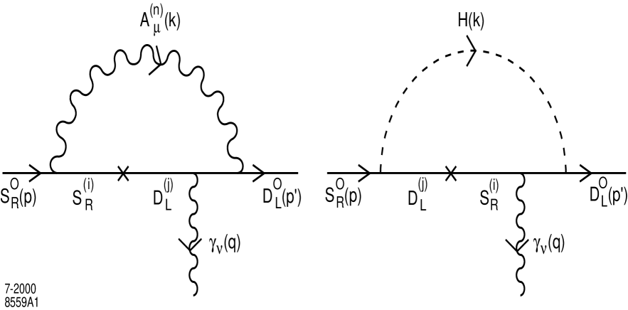
Figure 1: Typical Feynman diagrams for the gauge and Higgs boson contribution to $(g-2)_{\mu}$. The mass insertion is denoted by the cross.

Helicity flips play an important role in evaluating the contributions to $(g-2)_{\mu}$ since muon KK excitations are now propagating inside the loop. As is well-known, for non-chiral couplings the contribution to the anomalous magnetic moment of a light fermion can be enhanced when a heavy fermion of mass $m_{h}$ participates inside the loop[11]. There are a number of diagrams that can contribute to $(g-2)_{\mu}$ at one loop of which two are shown in Fig. 1. The diagram on the left corresponds to the exchange of a tower of the 4-d neutral gauge bosons, $\gamma^{(n)}$ and/or $Z^{(n)}$, which we will now discuss in detail. Due to gauge invariance we are free to choose a particular gauge in order to simplify the calculation. Here, we make use of the $\xi=1$ unitary gauge where the 4-d propagator is just the flat space metric tensor[12]. Hence, the loops with the 4-d components of the gauge fields and the ones with the fifth component need to be considered separately. In this example, the mass insertion takes place inside the loop before the photon is emitted. Clearly there are three other diagrams of this class: two with the mass insertion on an external leg and the third with the mass insertion inside the loop but after the photon is emitted. The amplitude arising from this vector exchange graph is given by

$${\cal M}_{V} = C_{L}C_{R}C_{0in}^{ffA}C_{0jn}^{ffA}~{}\bar{u}(p^{\prime})\ (-ie\gamma_{\mu})P_{L}i{{\hat{\not\!p^{\prime}}+m_{j}}\over{\hat{p}^{\prime 2}-m_{j}^{2}}}\ (-ie\gamma_{\nu})P_{L}\,$$ (4)

$$\times i{{\hat{\not\!p}+m_{j}}\over{\hat{p}^{2}-m_{j}^{2}}}\ (im_{ij}P_{R})\ i{{\hat{\not\!p}+m_{i}}\over{\hat{p}^{2}-m_{i}^{2}}}\ (-ie\gamma^{\mu})P_{R}\ u(p)\ {-i\over{k^{2}-m_{A}^{(n)~{}2}}}+h.c.\,,$$

where $C_{L,R}$ are the corresponding couplings of the SM gauge boson to the $\mu$ in units of $e$ and $\hat{p}(\hat{p}^{\prime})=p(p^{\prime})-k$. The coefficients $C_{0in}^{ffA}$ are the reduced couplings between a zero mode fermion, a fermion tower member of mass $m_{i}$ and the $n^{th}$ gauge boson tower member. Here $m_{i}$ and $m_{j}$ are the masses of the $D$ or $S$ fermionic KK states and $m_{A}^{(n)}$ are the masses of the KK gauge tower states. Note that the mass insertion, $m_{ij}$, comes with a chirality factor that can be determined from the action $S_{fH}$; numerically, $m_{ij}=C_{ij}^{ffH}v_{4}$. The amplitude where the mass insertion comes after the photon emission can be easily obtained by interchanging $i$ and $j$ in the resulting final amplitude expression. When the mass insertion occurs on an external leg it connects a zero mode with a tower mode and is given by $m_{0i}=C_{0i}^{ffH}v_{4}$. With some algebra it is straightforward to show that the corresponding amplitudes obtained in the two cases with external insertions are suppressed in comparison to the case of internal insertion by a factor of order $\sim m_{\mu}^{2}/M_{KK}^{2}$, where $M_{KK}$ is a typical large KK mass. In the case of the $W$ gauge boson tower graphs, since the $W$ couples only to the $D$’s, the mass insertion must occur on the incoming leg of the graph and the photon is emitted from the $W$; this graph can also be shown to produce a sub-leading contribution by a factor of order $\sim m_{\mu}^{2}/M_{KK}^{2}$. Thus, $W$ tower graphs can be safely ignored in comparison to those arising from the $Z$ and $\gamma$ towers and the resulting contribution from all of the 4-d vector exchanges, neglecting the subleading terms, is given by

$$\Delta a_{\mu}^{A} = \sum_{i,j,k}{-3C_{V}^{2}K\alpha m_{ij}m_{\mu}\over{\pi}}\times\,$$ (5)

$$\int_{0}^{1}~{}dx~{}\int_{0}^{1-x}~{}dy~{}\Bigg{[}{x(1-x-y)\over{m_{j}^{2}(1-x-y)+m_{i}^{2}y+m_{A}^{(k)2}x}}\ +(i\rightarrow j)\Bigg{]}\,,$$

where the sum is over all internal KK states, the $i\rightarrow j$ represents the addition of the other internal insertion graph and $C_{V}^{2}=C_{0ik}^{ffA}C_{0jk}^{ffA}$ with $K$ given by

$$K=\Bigg{[}1+{{(1-4x_{w})^{2}-1}\over{16x_{w}(1-x_{w})}}\Bigg{]}\,,$$ (6)

where $x_{w}=\sin^{2}\theta_{w}\simeq 0.2315$. Note that since the coefficients $C_{0ik}^{ffA}$ behave as $\sim 1/\sqrt{F}$[8] and $m_{ij}\sim F$ we may expect that the $\nu$ dependence of $\Delta a_{\mu}^{A}$ to be rather weak. In principle the sum extends over all of the internal KK states but in practice we find that truncating the sum after the first 20-40 members of each tower leads to a rather stable result.

The next class of graphs is similar to the 4-d vector exchange, but in the $\xi=1$ gauge, now involves the fifth component of the original 5-d field. Here it is important to recall that these fifth components are $Z_{2}$ odd fields thus connecting $S_{L}(D_{L})$ with $S_{R}(D_{R})$. The action $S_{fH}$ in Eq.(2) demonstrates that the Higgs boson does not interact with odd fields since they vanish on the wall. From this observation we conclude that in the case of fifth component vector exchanges the mass insertions can only occur on the external legs. By following similar algebraic manipulations as before it is easy to show that all of these contributions are always subleading by factors of order $\sim m_{\mu}^{2}/M_{KK}^{2}$ and thus their contribution to $(g-2)_{\mu}$ can be safely neglected.

Next, we turn to the possibility of Higgs exchange, also shown in Fig. 1. Ordinarily, one might dismiss such contributions as being small but they now involve the off-diagonal Higgs couplings discussed above which contain powers of the factor $F$ which grows large rapidly as $\nu$ grows negative. The amplitude for the Higgs graph shown in the figure is given by

$${\cal M}_{H} = C_{0i}^{ffH}C_{0j}^{ffH}~{}\bar{u}(p^{\prime})\ iP_{R}\ i{{\hat{\not\!p^{\prime}}+m_{i}}\over{\hat{p}^{\prime 2}-m_{i}^{2}}}(-ie\gamma_{\nu})P_{R}\ i{{\hat{\not\!p}+m_{i}}\over{\hat{p}^{2}-m_{i}^{2}}}\,$$ (7)

$$\times (im_{ij}P_{L})\ i{{\hat{\not\!p}+m_{j}}\over{\hat{p}^{2}-m_{j}^{2}}}\ iP_{R}\ u(p)\ {i\over{k^{2}-m_{H}^{2}}}\ +h.c.\,,$$

using the notation above. Here the coefficients $C_{0i}^{FFH}$ are the reduced couplings of a Higgs boson to a zero mode fermion and an $i^{th}$ fermion tower member. The amplitude where the insertion and emission occur with the opposite order can be obtained in a straightforward manner and, as we now expect, the two diagrams with external insertions can be shown to be subleading. Combining the two dominant Higgs amplitudes we find the following contribution to $\Delta a_{\mu}$:

$$\Delta a_{\mu}^{H}=\sum_{i,j}{C_{H}^{2}m_{ij}m_{\mu}\over{16\pi^{2}}}\ \int_{0}^{1}~{}dx~{}\int_{0}^{1-x}~{}dy~{}\Bigg{[}{{(1-x-y)(3y-3x-1)}\over{m_{i}^{2}(1-x-y)+m_{j}^{2}y+m_{H}^{2}x}}\ +(i\rightarrow j)\Bigg{]}\,,$$ (8)

where $C_{H}^{2}=C_{0i}^{ffH}C_{0j}^{ffH}$ with $m_{H}$ being the Higgs boson mass. The $i\rightarrow j$ term results from the addition of the other internal emission graph. (In our numerical analysis below we assume $m_{H}=120$ GeV; these results are not very sensitive to this particular choice.) Since $C_{0i}^{ffH}$ behave as $\sim\sqrt{F}$ and $m_{ij}\sim F$ we expect $\Delta a_{\mu}^{H}$ to have a strong $\nu$ dependence and to grow very rapidly as $\nu$ becomes increasingly negative. As in the vector case, truncating the sum over the KK fermion contributions after the first 20-40 tower members have been included yields a numerically stable result.

What are the other potential contributions to $(g-2)_{\mu}$ in the RS model? The radion is the zero mode remnant scalar resulting from the KK decomposition of the 5-d graviton field. Since it couples diagonally to KK tower members, as does the zero mode graviton and photon, the $\mu$ continues through the diagram and no KK modes are excited. Loops involving radions[13] are thus easily shown to be small[14] since both the radion couplings and the mass insertions in this case are not accompanied by any compensating powers of $F$. These contributions can be safely neglected.

The last remaining potential contribution arises from graviton loops which may be calculated via the Feynman rules given in [15] with small modifications due to the fact that the SM fields are now in the bulk and have nontrival $Z_{2}$ parity. These diagrams lead to amplitudes which are found to be log-divergent and lead to cutoff ($\Lambda$) dependent results and are thus not well-defined. The divergences, which occur in all graviton diagrams, arise due to the fact that the operator describing, e.g., the fermion-fermion-graviton interaction is dimension-five and involves an additional power of fermion momentum.

This differs significantly from the results obtained by Graesser [7] in the case of the ADD model, where it was found that the total contribution to $(g-2)_{\mu}$ due to gravity is finite. This difference arises from a number of sources: (i) in the ADD model the SM fields lie on the wall and only gravitons are allowed to propagate in the bulk, whereas in the version of the RS model under consideration here, both the SM gauge fields and fermions propagate in the bulk. (ii) In the ADD case, the graviton couplings are universal for all KK tower members whereas in the RS scenario the couplings are KK excitation state dependent and also differ for fermions and gauge bosons for arbitrary values of $\nu$. (iii) In the ADD case, each of the 5 diagrams shown in Fig. 1 of Graesser [7] was found to be log divergent with their sum, however, being finite, since the divergences cancel at each KK level. In the RS case, these cancellations cannot occur due to both the breakdown in universality of the graviton couplings and the fact that the complete calculation of each diagram involves different coupling coefficients and different numbers of KK states. For example, in the diagram where the graviton is emitted off the fermion KK line, we must sum over the triple product of coefficients $C_{0ik}^{ffG}C_{0jk}^{ffG}m_{ij}$. On the otherhand, the diagram involving the gauge-gauge graviton vertex we must instead sum over the quartic product of coefficients $C_{0ik}^{ffA}C_{0k\ell}^{AAG}C_{0n\ell}^{ffG}m_{in}$, where the sum extends over the KK towers for two fermions, one graviton, and one photon. Since the evaluation of the coefficients involve $\nu$-dependent integrals over Bessel functions, it is highly unlikely that the divergences encountered in each class of diagrams can sum to zero unless a theorem demands that it be so. Thus, we expect that the complete contribution due to gravity to remain log divergent when all diagrams are summed.

We can, however, make an estimate of the size of these graviton contributions. As in the case of vector and Higgs boson exchange we expect graphs with internal insertions proportional to $F$ to dominate. Since the relevant vertex couplings $C_{0ik}^{ffG}$ scale as $\sim 1/\sqrt{F}$[8] we do not expect the graviton contribution to be strongly $\nu$ dependent as was also the case for vector exchange. An order of magnitude estimate suggests that

$$\Delta a_{\mu}^{G}\simeq\sum_{ijk}{C_{0ik}^{ffG}C_{0jk}^{ffG}m_{ij}m_{\mu}\over{16\pi^{2}\Lambda_{\pi}^{2}}}\ log\Bigg{[}{\Lambda^{2}\over{m_{KK_{k}}^{2}}}\Bigg{]}\,,$$ (9)

with the cutoff $\Lambda$ expected to be of order $\Lambda_{\pi}$. The origin of the various terms in this estimate are easy to identify: the $C$’s are vertex functions, the $(16\pi^{2})^{-1}$ is a typical loop factor, the $\Lambda_{\pi}^{-1}$ appears in all graviton couplings to SM fields, and the $m_{ij}m_{\mu}$ arises in the usual single mass insertion approximation as seen above. The $\log\Lambda^{2}$ is the divergence discussed above and $m_{KK_{i}}$ represents canonical KK-tower masses which appear in the loop. Note that $\Lambda_{\pi}\rightarrow\infty$ as $m_{KK_{i}}\rightarrow\infty$ and thus $\Delta a_{\mu}^{G}\rightarrow 0$ as the KK mass gets large. Inserting typical values of the parameters we estimate that $\Delta a_{\mu}^{G}$ should certainly be less than $10^{-(9-10)}$ and thus is at most comparable to the vector boson contribution. (An explicit calculation of the diagram containing the $\gamma ffG$ vertex confirms this expectation.) As we will see this means that the graviton exchange contributions will then have very little effect upon our results.

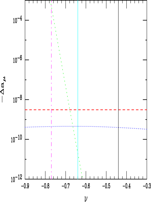
Figure 2: Bounds on the parameter $\nu$ from considerations of $(g-2)_{\mu}$. The horizontal dotted curve shows the value of $-\Delta a_{\mu}^{A}$ while the steeply rising dotted curve is that for $-\Delta a_{\mu}^{H}$; both of which are calculated assuming the mass of the first KK gauge state to be 1 TeV. The vertical dash dotted line arises from the Yukawa coupling perturbativity constraint discussed in the text while the left(right)solid line arises from the corresponding $\mu$(top) no fine-tuning mass constraint. Regions to the left of these lines are excluded. The horizontal dashed line is the current experimental upper bound at $95\%$ CL.

Let us now turn to our numerical results which are summarized in Fig. 2. We first remind the reader that for a fixed value of $\nu$ specifying the mass of any single KK tower state determines the entire KK spectrum for fermions, gauge bosons and gravitons. Here we take the mass of the lightest gauge KK state to be 1 TeV with the results for both the vector and Higgs contributions scaling as $\sim(1~{}{\rm TeV}/M_{KK})^{2}$. In our previous work[8] we have shown that for values of $\nu\mathrel{\mathchoice{\lower 3.01385pt\vbox{\halign{$\matth\displaystyle\hfil#\hfil$\cr>\crcr\sim\crcr}}}{\lower 3.01385pt\vbox{\halign{$\matth\textstyle\hfil#\hfil$\cr>\crcr\sim\crcr}}}{\lower 3.01385pt\vbox{\halign{$\matth\scriptstyle\hfil#\hfil$\cr>\crcr\sim\crcr}}}{\lower 3.01385pt\vbox{\halign{$\matth\scriptscriptstyle\hfil#\hfil$\cr>\crcr\sim\crcr}}}}-0.3$ the masses of the KK states as well as $\Lambda_{\pi}$ are required to be in the multi-TeV range, disfavoring this model as a solution to the hierarchy problem. Also we noted that when $\nu\mathrel{\mathchoice{\lower 3.01385pt\vbox{\halign{$\matth\displaystyle\hfil#\hfil$\cr<\crcr\sim\crcr}}}{\lower 3.01385pt\vbox{\halign{$\matth\textstyle\hfil#\hfil$\cr<\crcr\sim\crcr}}}{\lower 3.01385pt\vbox{\halign{$\matth\scriptstyle\hfil#\hfil$\cr<\crcr\sim\crcr}}}{\lower 3.01385pt\vbox{\halign{$\matth\scriptscriptstyle\hfil#\hfil$\cr<\crcr\sim\crcr}}}}-0.9$ the Yukawa couplings of the fermions became too large, hence for we display the range of $\nu$ in Fig. 2 to be between $-0.3$ and $-1$.

The first result to notice is the value of $\Delta a_{\mu}^{A}$ corresponding to the essentially $\nu$-independent horizontal dotted curve. This $\nu$ independence is only approximate and results from the scale of the figure as $\Delta a_{\mu}^{A}$ varies by a factor of order a few as $\nu$ increases up to 2. This curve lies about an order of magnitude below the current experimental $(g-2)_{\mu}$ bound implying that we should obtain no reasonable constraint on the KK masses arising from this contribution unless there is a substantial change in both the experimental central value and the error. The rising dotted line is the Higgs boson contribution which we note is rather small over most of the interesting range of $\nu$. Scaling the curve to allow for the first KK masses to only be as large as a few to 10 TeV, we find that the region to the left of $\nu\simeq-0.70$ is excluded. This rules out a reasonable fraction, $\simeq 30\%$, of the preferred allowed range of $\nu$ remaining subsequent to our last analysis[8].

There are however two other points to consider. First, a quick examination of the perturbative bound on the Yukawa couplings in the Higgs graph shown in Fig. 1 also yields a constraint. Imposing the weak requirement that $C_{H}^{2}=C_{0i}^{ffH}C_{0j}^{ffH}<16\pi^{2}$ we obtain the dash-dotted line in Fig. 2 at $\nu\simeq-0.77$ excluding the region to its left. A second, perturbative-like bound can also be extracted from the Higgs loop in Fig.1 when we remove the photon line and consider the resulting mass renormalization contribution[16]. We next demand the no fine-tuning requirement that the finite part of this graph be not much larger than $m_{\mu}$; from this we explicitly obtain the constraint that $C_{H}^{2}m_{ij}/16\pi^{2}$ be not much greater than $m_{\mu}$. This then excludes the region to the left of the solid line at $\nu\simeq-0.64$ and results in a stronger bound than that obtained from the present experimental value of $(g-2)_{\mu}$. Of course one could repeat this exercise for the case of the top quark provided the value of $\nu$ is universal. In this case, the value of $C_{H}^{2}m_{ij}$ is increased by the factor $(m_{t}/m_{\mu})^{2}$ and the resulting bound is drastically strengthened. We find that the region to the left of $\nu\simeq-0.44$ would now be excluded by this analysis; these considerations now exclude more than $\simeq 75\%$ of the previously preferred range of $\nu$ and leaves only the relatively narrow window between $-0.30$ and $-0.44$ as allowed. This would seem to greatly disfavor the possibility of the SM being in the RS bulk in the case of a universal mass parameter, $\nu$.

In conclusion the present experimental measurements of $(g-2)_{\mu}$ do not place significant constraints on localized gravity models with the SM field content in the bulk for most of the allowed range of $\nu$. However, requiring that one loop corrections to the fermion masses be of the same order as the measured fermion mass, so that no fine tuning of the parameters in the Lagrangian are necessary, severly constrains the allowed bulk mass parameter space. This result is obtained assuming that the value of $\nu$ is flavor independent and that the 5-d Yukawa couplings of the fermions are hierarchical. Given these assumptions, however, placing the SM field content in the bulk is tightly constrained by the above considerations.

Acknowledgements

The authors would like to thank S. Brodsky, S. Chivukula, Y. Grossman, J. Ng, M. Peskin, A. Pomarol, M. Schmaltz, and J.Wells for discussions related to this work.

References

- [1] N. Arkani-Hamed, S. Dimopoulos, and G. Dvali, Phys. Lett. B429, 263 (1998), and Phys. Rev. D59, 086004 (1999); I. Antoniadis, N. Arkani-Hamed, S. Dimopoulos, and G. Dvali, Phys. Lett. B436, 257 (1998).
- [2] L. Randall and R. Sundrum, Phys. Rev. Lett. 83, 3370 (1999), and ibid., 4690, (1999).
- [3] I. Antoniadis, Phys. Lett. B246, 377 (1990); I. Antoniadis, C. Munoz and M. Quiros, Nucl. Phys. B397, 515 (1993); I. Antoniadis and K. Benalki, Phys. Lett. B326, 69 (1994); I. Antoniadis, K. Benalki and M. Quiros, Phys. Lett. B331, 313 (1994).
- [4] G.F. Giudice, R. Rattazzi, and J.D. Wells, Nucl. Phys. B544, 3 (1999); E.A. Mirabelli, M. Perelstein, and M.E. Peskin, Phys. Rev. Lett. 82, 2236 (1999); T. Han, J.D. Lykken, and R.-J. Zhang, Phys. Rev. D59, 105006 (1999); J.L. Hewett, Phys. Rev. Lett. 82, 4765 (1999); T.G. Rizzo, Phys. Rev. D59, 115010 (1999). For a recent review, see T.G. Rizzo, hep-ph/9910255.
- [5] H. Davoudiasl, J.L. Hewett, and T.G. Rizzo, Phys. Rev. Lett. 84, 2080 (2000).
- [6] For a recent review of the experimental and theoretical situation, see R. Carey, talk given at the XXXth International Conference on High Energy Physics, Osaka, Japan, July 27-August 2, 2000.
- [7] M.L. Graesser, Phys. Rev. D61, 074019 (2000). See also, P. Nath and M. Yamaguchi, Phys. Rev. D60,, 116006 (1999).
- [8] H. Davoudiasl, J.L. Hewett, and T.G. Rizzo, Phys. Lett. B473, 43 (2000), and hep-ph/0006041.
- [9] W.D. Goldberger and M.B. Wise, Phys. Rev. Lett. 83, 4922 (1999); O. DeWolfe, D.Z. Freedman, S.S. Gubser, and A. Karch, hep-th/9909134; M.A. Luty, and R. Sundrum, hep-ph/9910202; J. Garriga, O. Pujolàs, and T. Tanaka, hep-ph/0004109; U. Mahanta, hep-ph/0006350; W.D. Goldberger and I.Z. Rothstein, hep-th/0007065; C. Csaki, M. Graesser, L. Randall, and J. Terning, Phys. Rev. D62, 045015 (2000).
- [10] A. Pomarol, hep-ph/9911294; S. Chang and M. Yamaguchi, hep-ph/9909523; Y. Grossman and M. Neubert, Phys. Lett. B474, 361 (2000); R. Kitano, hep-ph/0002279; S. Chang et al., hep-ph/9912498; T. Gherghetta and A. Pomarol, hep-ph/0003129; S.J. Huber and Q. Shafi, hep-ph/0005286; C-H. V. Chang and J.N. Ng, hep-ph/0006164.
- [11] S.J. Brodsky and J.D. Sullivan, Phys. Rev. 156, 1644 (1967) ; S.J. Brodsky and S. Drell, Phys. Rev. D22, 2236 (1980).
- [12] See, for example, A. Delgado, A. Pomarol and M. Quiros, Phys. Rev. D60, 095008 (1999).
- [13] W.D. Goldberger and M.B. Wise, hep-ph/9911457; U. Mahanta and S. Rakshit, hep-ph/0002049; U. Mahanta and A. Datta, hep-ph/0002183; G.F. Giudice, R. Rattazzi and J.D. Wells, hep-ph/0002178; J.E. Kim, B. Kyae and J.D. Park, hep-ph/0007008.
- [14] See the last paper of the previous reference.
- [15] For the Feynman rules, see the first three papers in Ref. [4].
- [16] We would like to thank S. Chivukula for pointing out this constraint to us.