Leading logarithm calculation of the
$e^{+}e^{-}\rightarrow e^{+}\,\nu_{e}\,\bar{u}\,d$ cross section

Abstract

We analytically evaluate in the leading logarithm approximation the differential cross section for $e^{+}e^{-}\rightarrow e^{+}\,\nu_{e}\,\bar{u}\,d$. We compare our order $\alpha^{4}\alpha_{s}^{0}$ leading-log result to the order $\alpha^{4}\alpha_{s}^{0}$ exact result obtained from the GRC4F Monte Carlo program. Finally we use the Glück, Reya, Schienbien distribution of partons in a virtual photon, which incorporates both evolution and nonperturbative strong interaction contributions, to obtain better estimates of the differential cross section.

I Introduction

Events at a high energy $e^{+}e^{-}$ collider in which only hadrons are seen in the final state and the net momemtum of the hadrons transverse to the beam axis is large could be signatures for physics beyond the standard model [1]. However, these events could also arise from the simple standard model process depicted in Fig. 1. Here the positron emits a slightly virtual photon and escapes down the beam pipe. The hadrons recoil against a high $P_{T}$ neutrino.

The cross section for background processes that arise from graphs like that shown in Fig. 1 can be computed exactly to order $\alpha^{4}\alpha_{s}^{0}$ by using the Monte Carlo code GRC4F [2]. However, it is useful to have an approximate analytical calculation of the cross section as a check, if the calculation is simple enough to illuminate the basic physics. In this paper, we provide such a calculation based on the leading logarithm approximation in which the photon carries small transverse momentum $p_{T}$ while the quark carries much larger transverse momentum $k_{T}$: $m_{e}^{2}\ll p_{T}^{2}\ll k_{T}^{2}\ll M_{W}^{2}$. We compare our order $\alpha^{4}\alpha_{s}^{0}$ leading-log result with the order $\alpha^{4}\alpha_{s}^{0}$ exact result.

We also go beyond the $\alpha^{4}\alpha_{s}^{0}$ leading-log result by incorporating two strong interaction effects: the DGLAP evolution of parton distribution functions in a virtual photon giving rise to contributions of order $\sum_{N}(\alpha_{s}\ln Q^{2}/|p^{2}|)^{N}$, and the phenomenological, nonperturbative splitting of the photon into a quark plus anything. To that end, we use the Glück, Reya and Schienbein (GRS) parton distributions in a virtual photon [3]. We investigate whether these two strong interaction effects are big enough to substantially affect the cross section.

FIG. 1.: Charged current deep inelastic scattering $e^{+}e^{-}\rightarrow e^{+}\nu_{e}\,\bar{u}\,d$.

.

II Framework

In this section, we set the framework for the approximations we will make and the momentum cuts we will use. We first present notation that will prove useful later on in the calculation. We will use light-cone coordinates [4] to describe momentum four-vectors $p^{\mu}$,

$$p^{\pm}=\frac{p^{0}\pm p^{3}}{\sqrt{2}},\ \ \ p_{T}^{j}=(p^{1},p^{2}).$$ (1)

This set of coordinates is very convenient for symmetric collisions because one of the incoming particles has almost exclusively plus momentum and negligible minus and transverse momentum, whereas the other has almost exclusively minus momentum.

There are constraints on the momenta of the photon and the quark coupling to the W boson. As the transverse momentum squared $p_{T}^{2}$ of the photon falls below the mass squared $m_{e}^{2}$ of the positron, the matrix element squared falls off sharply. We can thus take $m_{e}^{2}$ to be an effective lower limit of integration for $p_{T}^{2}$. Its upper limit is the squared veto momentum of positron detection, $M^{2}$. This is an experimental limit and will depend on the exact configuration of the detector. If the scattered positron has an angle $\theta$ greater than some limit $\theta_{0}$, it will be detected. Thus we demand that $|\theta|<\theta_{0}$. In our approximate calculation, this amounts to requiring that $p_{T}<M=\theta_{0}\sqrt{s}/2$.

A reasonable lower cut-off on the quark transverse momentum squared $k_{T}^{2}$ is the greater of $m_{\rho}^{2}$, the mass squared of the $\rho$ meson (or indeed some other meson such as the $\pi$), and $p_{T}^{2}$, i.e. $k_{T}^{2}>\max(m_{\rho}^{2},p_{T}^{2})$. For $k_{T}^{2}<m_{\rho}^{2}$, the distribution function of quarks in a photon is nonperturbative. In the first part of this investigation, we have set this nonperturbative contribution to zero. The approximate upper limit on $k_{T}^{2}$ is the virtuality of the W boson, $Q^{2}$, which is fixed by the transverse momentum of the neutrino. A plot of these constraints, Fig. 2, makes it easy to visualize the phase-space under consideration.

FIG. 2.: Momentum cuts.

The approximation we make is to calculate the cross section by including the region in the middle of the polygon in Fig. 2, without worrying about what happens at its edges. This is reasonable because most events will lie in this region,

$$m_{e}^{2}\ll p_{T}^{2}\ll k_{T}^{2}\ll Q^{2}.$$ (2)

This approximation is called the leading-log approximation, for reasons that will become apparent later on. We can split our calculation into three steps, in which the hardness increases at each step.

The first step is to assume that the transverse momentum $p_{T}$ of the photon is much smaller than the transverse momentum $k_{T}$ of the quark that couples the photon to the W boson (Graph A, Fig. 3). We can then calculate the piece of Fig. 1 dealing with the emission of the photon from the positron. The second step is to assume that the transverse momentum $k_{T}$ of the quark is much smaller than the transverse momentum $q_{T}$ of the W boson (Graph B, Fig. 4). We then calculate the piece of Fig. 1 in which the photon splits into a quark-antiquark pair. The third and final step involves no further approximations and is a direct calculation of the cross section for charged current deep inelastic scattering (Graph C, Fig. 5).

The general form of the cross section for the process in Fig. 1 is the following:

$$d\sigma = \frac{1}{2P^{0}2l^{0}2}|{\mathcal{M}}_{\mathrm{A}}|^{2}\frac{d^{2}P^{\prime}_{T}dP^{\prime+}}{(2\pi)^{3}2P^{\prime+}}\frac{d^{2}l^{\prime}_{T}dl^{\prime+}}{(2\pi)^{3}2l^{\prime+}}\frac{d^{2}k^{\prime}_{T}dk^{\prime+}}{(2\pi)^{3}2k^{\prime+}}\frac{d^{2}k^{\prime\prime}_{T}dk^{\prime\prime+}}{(2\pi)^{3}2k^{\prime\prime+}}$$ (4)

$$\times(2\pi)^{4}\delta^{4}(P^{\mu}+l^{\mu}-P^{\prime\mu}-l^{\prime\mu}-k^{\prime\mu}-k^{\prime\prime\mu}).$$

We are now ready to calculate the total matrix element squared.

III Graph A: Calculation of $P_{\gamma/e}$

As just discussed, we will calculate the total matrix element squared $|{\mathcal{M}}_{\mathrm{A}}|^{2}$ in three successive refinements. First we concentrate on the part of the diagram involving the photon (Graph A, Fig. 3), which will be the starting point. This is the first step in our three-step calculation, as we go from the least hard to the most hard part of the diagram in Fig. 1. $|{\mathcal{M}}_{\mathrm{A}}|^{2}$ will contain a factor $|{\mathcal{M}}_{\mathrm{B}}|^{2}$ that represents the next hardest contribution, while $|{\mathcal{M}}_{\mathrm{B}}|^{2}$ will contain the very hardest factor $|{\mathcal{M}}_{\mathrm{C}}|^{2}$.

FIG. 3.: Graph A.

We calculate the probability $P_{\gamma/e}$ of finding a photon in a positron by evaluating Graph A (Fig. 3). Averaging over the initial spins of the positron, we find the total matrix element squared to be

$$|{\mathcal{M}}_{A}|^{2}=\frac{e^{2}}{(p^{2})^{2}}\frac{1}{2}\sum_{i,j}\mathrm{Tr}\left\{\!\not\!{P}\!\not\!{\epsilon}(p,j)\!\not\!{P}^{\prime}\!\not\!{\epsilon}(p,i)\right\}\delta^{ij}|{\mathcal{M}}_{B}|^{2}.$$ (5)

Here we neglect the positron mass compared to $p_{T}$. $|{\mathcal{M}}_{B}|^{2}$ is averaged over the photon polarizations and contains the next hardest part which we calculate later on. $\epsilon(p,i)$ is the polarization vector in the physical $A^{+}=0$ gauge of the photon with momentum $p^{\mu}$ and polarization index $i$.

We work in the c.m. frame of the electron and positron, with the positron carrying only plus momentum and the electron carrying only minus momentum. In this frame the momenta in our graphs have components $v^{\nu}=(v^{+},v^{-},\vec{v}_{T})$ given by

$$P^{\mu} = (P^{+},0,\vec{0}_{T}),$$ (6)

$$l^{\mu} = (0,l^{-},\vec{0}_{T}),$$ (7)

$$P^{\prime\mu} = \left((1-\xi)P^{+},\frac{p_{T}^{2}}{2(1-\xi)P^{+}},-\vec{p}_{T}\right),$$ (8)

$$p^{\mu} = \left(\xi P^{+},\frac{-p_{T}^{2}}{2(1-\xi)P^{+}},\vec{p}_{T}\right).$$ (9)

Now, $\epsilon^{\mu}(p,i)$ is

$$\epsilon^{+}(p,i)=0,\ \ \ \epsilon^{-}(p,i)=p_{T}\cdot\epsilon_{T}/p^{+},\ \ \ \epsilon^{j}(p,i)=\delta_{i}^{j}.$$ (10)

Using $\sum_{i}\epsilon^{2}(p,i)=-2$, we have

$$|{\mathcal{M}}_{\mathrm{A}}|^{2}=\frac{4(2\pi)\alpha}{p_{T}^{2}}\frac{(1-\xi)}{\xi}\left\{\frac{1+(1-\xi)^{2}}{\xi}\right\}|{\mathcal{M}}_{\mathrm{B}}|^{2}.$$ (11)

We recognize the standard splitting function $P_{\gamma/e}$,

$$P_{\gamma/e}(\xi)=\frac{1+(1-\xi)^{2}}{\xi}.$$ (12)

Define $p^{\mu}\approx\tilde{p}^{\mu}\equiv(\xi P^{+},0,\vec{0}_{T})$. Since the process is very hard, i.e. $p_{T}\ll k_{T}$, the minus components and transverse components of $p^{\mu}$ are small compared to the plus components. In this approximation,

$$(2\pi)^{4}\delta^{4}(P^{\mu}+l^{\mu}-P^{\prime\mu}-l^{\prime\mu}-k^{\prime\mu}-k^{\prime\prime\mu})\approx(2\pi)^{4}\delta^{4}(\tilde{p}^{\mu}+l^{\mu}-l^{\prime\mu}-k^{\prime\mu}-k^{\prime\prime\mu}).$$ (13)

Then the cross section can be reexpressed to depend on $p_{T}$ and $\xi$,

$$d\sigma = \frac{2\alpha d^{2}p_{T}d\xi}{(2\pi)^{2}p_{T}^{2}}P_{\gamma/e}(\xi)\frac{1}{2\tilde{p}^{0}2l^{0}2}|{\mathcal{M}}_{\mathrm{B}}|^{2}\frac{d^{2}l^{\prime}_{T}dl^{\prime+}}{(2\pi)^{3}2l^{\prime+}}\frac{d^{2}k^{\prime}_{T}dk^{\prime+}}{(2\pi)^{3}2k^{\prime+}}\frac{d^{2}k^{\prime\prime}_{T}dk^{\prime\prime+}}{(2\pi)^{3}2k^{\prime\prime+}}$$ (15)

$$\times(2\pi)^{4}\delta^{4}(\tilde{p}^{\mu}+l^{\mu}-l^{\prime\mu}-k^{\prime\mu}-k^{\prime\prime\mu}).$$

IV Graph B: Calculation of $P_{q/\gamma}$

We now calculate the probability of finding a quark in a photon. This will give us $|{\mathcal{M}}_{\mathrm{B}}|^{2}$, in terms of the final hard matrix element squared $|{\mathcal{M}}_{\mathrm{C}}|^{2}$. There is also a graph $\mathrm{B}^{\prime}$ in which the quark is replaced by an antiquark. In this case, everything is the same except the hard matrix element $|{\mathcal{M}}_{\mathrm{C}}|^{2}$ is replaced by a different matrix element $|{\mathcal{M}}_{\mathrm{C}^{\prime}}|^{2}$.

FIG. 4.: Graph B.

Summing over colors and averaging over spins, the matrix element squared for Graph B (Fig. 4) is

$$|{\mathcal{M}}_{\mathrm{B}}|^{2}=N_{C}\frac{e_{q}^{2}e^{2}}{(k^{2})^{2}}\frac{1}{2}\sum_{i}\mathrm{Tr}\left\{{\mathcal{H}}\!\not\!{k}\!\not\!{\epsilon}(\tilde{p},i)\!\not\!{k}^{\prime\prime}\!\not\!{\epsilon}(\tilde{p},i)\!\not\!{k}\right\}.$$ (16)

Again, the mass of the quark is negligible compared to $k_{T}$. The matrix ${\mathcal{H}}$ contains the final contribution that we will evaluate using Graph C (Fig. 5) later on. For now, we leave it as it is. Let $\!\not\!{L}=\!\not\!{k}\!\not\!{\epsilon}(\tilde{p},i)\!\not\!{k}^{\prime\prime}\!\not\!{\epsilon}(\tilde{p},i)\!\not\!{k}$. Since the partons involved are going much faster in the plus direction compared to all other directions, we can make the approximation $\!\not\!{L}\approx L^{+}\gamma^{-}$. Then,

$$|{\mathcal{M}}_{\mathrm{B}}|^{2}=N_{C}\frac{e_{q}^{2}e^{2}}{(k^{2})^{2}}\frac{1}{2}\sum_{i}\mathrm{Tr}\left\{{\mathcal{H}}\gamma^{-}\right\}L^{+}.$$ (17)

Let $\tilde{k}^{\mu}=(k^{+},0,\vec{0}_{T})$. We use it to rewrite the above,

$$|{\mathcal{M}}_{\mathrm{B}}|^{2}=N_{C}\frac{e_{q}^{2}e^{2}}{(k^{2})^{2}}\frac{1}{2}\sum_{i}\mathrm{Tr}\left\{{\mathcal{H}}\!\not\!{\tilde{k}}\right\}\frac{L^{+}}{k^{+}},$$ (18)

$$L^{+}=\frac{1}{4}\mathrm{Tr}\left\{\gamma^{+}L\right\}=\frac{1}{4}\mathrm{Tr}\left\{\gamma^{+}\!\not\!{k}\!\not\!{\epsilon(\tilde{p},i)}\!\not\!{k}^{\prime\prime}\!\not\!{\epsilon(\tilde{p},i)}\!\not\!{k}\right\}.$$ (19)

The hard scattering matrix element squared, which we leave unevaluated for now, is $|{\mathcal{M}}_{\mathrm{C}}|^{2}=\frac{1}{2}\mathrm{Tr}\left\{{\mathcal{H}}\!\not\!{\tilde{k}}\right\}$, and the matrix element squared is in the simple form

$$|{\mathcal{M}}_{\mathrm{B}}|^{2}=N_{C}\frac{e_{q}^{2}e^{2}}{(k^{2})^{2}}\sum_{i}\frac{1}{4}\frac{1}{k^{+}}\mathrm{Tr}\left\{\gamma^{+}\!\not\!{k}\!\not\!{\epsilon(\tilde{p},i)}\!\not\!{k}^{\prime\prime}\!\not\!{\epsilon(\tilde{p},i)}\!\not\!{k}\right\}|{\mathcal{M}}_{\mathrm{C}}|^{2}.$$ (20)

In the same c.m. frame as earlier, but now with the approximation $p^{\mu}\rightarrow\tilde{p}^{\mu}$ described above,

$$p^{\mu} = (p^{+},0,\vec{0}_{T}),$$ (21)

$$k^{\mu} = \left(zp^{+},\frac{-k_{T}^{2}}{2(1-z)p^{+}},\vec{k}_{T}\right),$$ (22)

$$k^{\prime\prime\mu} = \left((1-z)p^{+},\frac{k_{T}^{2}}{2(1-z)p^{+}},-\vec{k}_{T}\right).$$ (23)

After doing the trace algebra, the matrix element squared is

$$|{\mathcal{M}}_{\mathrm{B}}|^{2}=\frac{4(2\pi)\alpha}{k_{T}^{2}}\frac{(1-z)}{z}e_{q}^{2}N_{C}\left\{z^{2}+(1-z)^{2}\right\}|{\mathcal{M}}_{\mathrm{C}}|^{2}.$$ (24)

We recognize the standard splitting function $P_{q/\gamma}$,

$$P_{q/\gamma}(z)=N_{C}\left\{z^{2}+(1-z)^{2}\right\}.$$ (25)

In the same approximation as before, the minus and transverse components being small compared to the plus components, the delta function in the cross section can be expressed as

$$(2\pi)^{4}\delta^{4}(\tilde{p}^{\mu}+l^{\mu}-l^{\prime\mu}-k^{\prime\mu}-k^{\prime\prime\mu})\approx(2\pi)^{4}\delta^{4}(\tilde{k}^{\mu}+l^{\mu}-l^{\prime\mu}-k^{\prime\mu}).$$ (26)

Let $x=k^{+}/P^{+}$, which implies $k^{+}=(x/\xi)p^{+}$ and $z=x/\xi$. Then, using the result we obtained for $|{\mathcal{M}}_{\mathrm{B}}|^{2}$, the cross section can be written as

$$d\sigma = \frac{4\alpha^{2}e_{q}^{2}}{(2\pi)^{4}}\frac{d\xi}{\xi}dxP_{\gamma/e}(\xi)P_{q/\gamma}(x/\xi)\frac{d^{2}p_{T}}{p_{T}^{2}}\frac{d^{2}k_{T}}{k_{T}^{2}}$$ (28)

$$\times\frac{1}{2\tilde{k}^{0}2l^{0}2}|{\mathcal{M}}_{\mathrm{C}}|^{2}\frac{d^{2}l^{\prime}_{T}dl^{\prime+}}{(2\pi)^{3}2l^{\prime+}}\frac{d^{2}k^{\prime}_{T}dk^{\prime+}}{(2\pi)^{3}2k^{\prime+}}(2\pi)^{4}\delta^{4}(\tilde{k}^{\mu}+l^{\mu}-l^{\prime\mu}-k^{\prime\mu}),$$

which makes it obvious that the cross section is the convolution of a hard-scattering cross section with a piece that we identify as the distribution function of a quark in a positron.

A brief description of the required distribution functions is relevant. Graph A (Fig. 3) involves the distribution function of the photon in the positron, and Graph B (Fig. 4) the distribution function of a quark in a photon. As we combine the two graphs, we will require the distribution function of a quark in a positron. We will perform the trivial angular integral to write $d^{2}p_{T}=\pi dp_{T}^{2}$. We now define the distribution functions described,

$$f_{\gamma/e}(x) = \frac{\alpha}{2\pi}\int_{m_{e}^{2}}^{M^{2}}\frac{dp_{T}^{2}}{p_{T}^{2}}P_{\gamma/e}(x),$$ (29)

$$f_{q/\gamma}(x,Q^{2},p_{T}^{2}) = \frac{\alpha e_{q}^{2}}{2\pi}\int_{\max(p_{T}^{2},m_{\rho}^{2})}^{Q^{2}}\frac{dk_{T}^{2}}{k_{T}^{2}}P_{q/\gamma}(x),$$ (30)

$$f_{q/e}(x,Q^{2}) = \frac{\alpha^{2}e_{q}^{2}}{(2\pi)^{2}}\int_{x}^{1}\frac{d\xi}{\xi}P_{\gamma/e}(\xi)P_{q/\gamma}(x/\xi)\int_{m_{e}^{2}}^{M^{2}}\frac{dp_{T}^{2}}{p_{T}^{2}}\int_{\max(p_{T}^{2},m_{\rho}^{2})}^{Q^{2}}\frac{dk_{T}^{2}}{k_{T}^{2}}.$$ (31)

We first evaluate the convolution of the splitting functions,

$$\int_{x}^{1}\frac{d\xi}{\xi}P_{\gamma/e}(\xi)P_{q/\gamma}(x/\xi)=N_{C}\left((1-x)+2(1+x)\ln x+\frac{4}{3}\frac{(1-x^{3})}{x}\right).$$ (32)

Next, we compute the momentum integral, either by inspection of Fig. 2, or by explicit calculation,

$$\int_{m_{e}^{2}}^{M^{2}}\frac{dp_{T}^{2}}{p_{T}^{2}}\int_{\max(p_{T}^{2},m_{\rho}^{2})}^{Q^{2}}\frac{dk_{T}^{2}}{k_{T}^{2}} = \ln\frac{Q^{2}}{m_{\rho}^{2}}\ln\frac{m_{\rho}^{2}}{m_{e}^{2}}+\ln\frac{Q^{2}}{M^{2}}\ln\frac{M^{2}}{m_{\rho}^{2}}+\frac{1}{2}\ln^{2}\frac{M^{2}}{m_{\rho}^{2}}.$$ (33)

Therefore, the distribution function of a quark in a positron (or, equivalently, in an electron) is

$$f_{q/e}(x,Q^{2})=\frac{\alpha^{2}e_{q}^{2}}{(2\pi)^{2}}N_{C}\left((1-x)+2(1+x)\ln x+\frac{4}{3}\frac{(1-x^{3})}{x}\right)$$ (34)

$$\times\left(\ln\frac{Q^{2}}{m_{\rho}^{2}}\ln\frac{m_{\rho}^{2}}{m_{e}^{2}}+\ln\frac{Q^{2}}{M^{2}}\ln\frac{M^{2}}{m_{\rho}^{2}}+\frac{1}{2}\ln^{2}\frac{M^{2}}{m_{\rho}^{2}}\right).$$ (35)

If we use phenomenological distribution functions $f_{q/\gamma}$ of quarks in virtual photons (e.g. GRS distribution functions), we can evaluate $f_{q/e}$ as

$$f_{q/e}(x,Q^{2}) = \frac{\alpha}{2\pi}\int_{x}^{1}\frac{d\xi}{\xi}\int_{m_{e}^{2}}^{M^{2}}\frac{dp_{T}^{2}}{p_{T}^{2}}P_{\gamma/e}(x/\xi)f_{q/\gamma}(\xi,Q^{2},p_{T}^{2}).$$ (36)

We will use this convolution in a following section when using the GRS distribution functions.

We label the hard scattering cross section $d\hat{\sigma}$,

$$d\hat{\sigma}=\frac{1}{2\tilde{k}^{0}2l^{0}2}|{\mathcal{M}}_{\mathrm{C}}|^{2}\frac{d^{2}l^{\prime}_{T}dl^{\prime+}}{(2\pi)^{3}2l^{\prime+}}\frac{d^{2}k^{\prime}_{T}dk^{\prime+}}{(2\pi)^{3}2k^{\prime+}}(2\pi)^{4}\delta^{4}(\tilde{k}^{\mu}+l^{\mu}-l^{\prime\mu}-k^{\prime\mu}).$$ (37)

The cross section $d\sigma$ is a convolution of the distribution function with the hard scattering cross section

$$d\sigma=\int dx\,f_{q/e}(x)\,d\hat{\sigma}.$$ (38)

V Graph C: Charged current deep inelastic scattering

The third and final part of the calculation is to compute the charged current deep inelastic scattering cross section, Graph C (Fig. 5). This final calculation is quite standard and involves no further approximations. It is a direct calculation of the Feynman diagrams in Fig. 5. It involves the W boson coupling constant $g_{W}=\sqrt{4\pi\alpha}/\sin\theta_{W}$ and the element of the quark mixing matrix $V_{ud}$ that relates the up quark to the down quark.

Graph C	Graph $\mathrm{C}^{\prime}$

FIG. 5.: Charged current deep inelastic scattering.

Averaging over initial spins, the matrix element squared for Graph C (Fig. 5) is

$$|{\mathcal{M}}_{\mathrm{C}}|^{2} = \frac{2\hat{s}^{2}(2\pi)^{2}\alpha^{2}|V_{ud}|^{2}}{\sin^{4}\theta_{W}(Q^{2}+M_{W}^{2})^{2}},$$ (39)

where $\hat{s}$ is the c.m. energy squared of the electron-quark system.

The calculation of the matrix element squared for an incoming antiquark instead of a quark is nearly identical, and is depicted in Graph $\mathrm{C}^{\prime}$, Fig. 5. The matrix element squared is

$$|{\mathcal{M}}_{\mathrm{C}^{\prime}}|^{2} = \frac{2\hat{s}^{2}(2\pi)^{2}\alpha^{2}|V_{ud}|^{2}}{\sin^{4}\theta_{W}(Q^{2}+M_{W}^{2})^{2}}(1-y)^{2},$$ (40)

where $y\equiv q\cdot P/l\cdot P$.

We are now ready to evaluate the hard scattering cross section. We first rewrite it in a more suitable form,

$$d\hat{\sigma} = \frac{1}{2\tilde{k}^{0}2l^{0}2}\frac{d^{2}l^{\prime}_{T}}{(2\pi)^{2}}\frac{dl^{\prime+}}{2l^{\prime+}}\delta(k^{\prime 2})|{\mathcal{M}}_{\mathrm{C}}|^{2}.$$ (41)

Now,

$$k^{\prime 2}=(k+q)^{2}=2xq\cdot P-Q^{2}=Q^{2}(x/x_{bj}-1),$$ (42)

where $x_{bj}\equiv Q^{2}/2q\cdot P$. We express the momentum $l^{\prime}$ of the outgoing lepton in terms of its transverse momentum $l^{\prime}_{T}$ and its pseudo-rapidity $\eta^{\prime}$,

$$l^{\prime\mu}=\left(l^{\prime}_{T}e^{\eta^{\prime}}/\sqrt{2},l^{\prime}_{T}e^{-\eta^{\prime}}/\sqrt{2},l^{\prime}_{T}\right),$$ (43)

so $dl^{\prime+}=l^{\prime+}d\eta^{\prime}$. The azimuthal angle integral is trivial, $d^{2}l^{\prime}_{T}=\pi dl_{T}^{\prime 2}$. In terms of the c.m. energy of the hard process, $k^{0}l^{0}=\hat{s}/4$.

The hard cross section is then

$$d\hat{\sigma}=\frac{1}{16\pi\hat{s}}\frac{x_{bj}}{Q^{2}}dl_{T}^{\prime 2}d\eta^{\prime}\delta(x-x_{bj})|{\mathcal{M}}_{\mathrm{C}}|^{2}.$$ (44)

Using the squared matrix elements $|{\mathcal{M}}_{\mathrm{C}}|^{2}$ and $|{\mathcal{M}}_{\mathrm{C}^{\prime}}|^{2}$ we calculated previously, and the fact that $Q^{2}=y\hat{s}$, we obtain

$$d\hat{\sigma}_{e^{-}u\rightarrow\nu_{e}d} = \frac{\pi\alpha^{2}|V_{ud}|^{2}}{2\sin^{4}\theta_{W}(Q^{2}+M_{W}^{2})^{2}}\frac{x}{y}dl_{T}^{\prime 2}d\eta^{\prime}\delta(x-x_{bj}),$$ (45)

$$d\hat{\sigma}_{e^{-}\bar{d}\rightarrow\nu_{e}\bar{u}} = \frac{\pi\alpha^{2}|V_{ud}|^{2}}{2\sin^{4}\theta_{W}(Q^{2}+M_{W}^{2})^{2}}\frac{x}{y}dl_{T}^{\prime 2}d\eta^{\prime}\delta(x-x_{bj})(1-y)^{2}.$$ (46)

VI Differential cross sections

We have computed all the pieces necessary for the calculation of the cross section,

$$d\sigma=\int dx\left\{f_{u/e}(x)d\hat{\sigma}_{e^{-}u\rightarrow\nu_{e}d}+f_{\bar{d}/e}(x)d\hat{\sigma}_{e^{-}\bar{d}\rightarrow\nu_{e}\bar{u}}\right\}.$$ (47)

The result is

$$\frac{d\sigma}{dl_{T}^{\prime 2}d\eta^{\prime}}=\frac{\alpha^{4}N_{C}|V_{ud}|^{2}}{8\pi\sin^{4}\theta_{W}(Q^{2}+M_{W}^{2})^{2}}\left(\frac{1}{2}\ln^{2}\frac{M^{2}}{m_{\rho}^{2}}+\ln\frac{M^{2}}{m_{\rho}^{2}}\ln\frac{m_{\rho}^{2}}{m_{e}^{2}}+\ln\frac{Q^{2}}{M^{2}}\ln\frac{M^{2}}{m_{e}^{2}}\right)$$ (48)

$$\times\left(x(1-x)+2x(1+x)\ln x+\frac{4}{3}(1-x^{3})\right)\left(\frac{e_{u}^{2}+e_{\bar{d}}^{2}(1-y)^{2}}{y}\right).$$ (49)

It is often more convenient to rexpress this in terms of $l_{T}^{\prime}$ rather than $l_{T}^{\prime 2}$,

$$\frac{d\sigma}{dl_{T}^{\prime}d\eta^{\prime}}=(2l_{T}^{\prime})\frac{d\sigma}{dl_{T}^{\prime 2}d\eta^{\prime}}.$$ (50)

The final step is to change variables from $x,y,Q^{2}$ to $\eta^{\prime},l_{T}^{\prime},s$ where $s$ is the c.m. energy squared of the $e^{+}e^{-}$ pair, not to be confused with the hard scattering c.m. energy squared $\hat{s}$. In the laboratory frame, neglecting $m_{e}$ in the change of variables,

$$P^{\mu} = \left(\sqrt{s/2},0,\vec{0}_{T}\right),$$ (51)

$$l^{\mu} = \left(0,\sqrt{s/2},\vec{0}_{T}\right),$$ (52)

$$l^{\prime\mu} = \left(\frac{l^{\prime}_{T}e^{\eta^{\prime}}}{\sqrt{2}},\frac{l^{\prime}_{T}e^{-\eta^{\prime}}}{\sqrt{2}},\vec{l}^{\prime}_{T}\right).$$ (53)

The change of variables is

$$Q^{2} = -(l-l^{\prime})^{2}=e^{\eta^{\prime}}l_{T}^{\prime}\sqrt{s},$$ (54)

$$x = \frac{Q^{2}}{2q\cdot P}=\frac{e^{\eta^{\prime}}l_{T}^{\prime}}{\sqrt{s}-e^{-\eta^{\prime}}l_{T}^{\prime}},$$ (55)

$$y = \frac{q\cdot P}{l\cdot P}=1-\frac{l_{T}^{\prime}e^{-\eta^{\prime}}}{\sqrt{s}}.$$ (56)

The physical region is where $x<1$:

$$2l_{T}^{\prime}\cosh\eta^{\prime}<\sqrt{s}.$$ (57)

We now have a simple approximation to the cross section that can be compared with the output of Monte Carlo programs. We check our cross section against GRC4F [2]. Later we introduce a refinement not included in the purely perturbative Monte Carlo calculation. From GRC4F, we obtain the momentum four-vectors of all final state particles for 3666 events of the type we are interested in corresponding to a luminosity ${\mathrm{L}}=100\ {\mathrm{pb}}^{-1}$. The c.m. energy is $\sqrt{s}=189\ {\mathrm{GeV}}$ and the veto momentum squared was taken to be $M^{2}=5\ {\mathrm{GeV^{2}}}$. To be consistent with the choice made in getting the GRC4F results, we pick the cut-off for the pertubative treatment of our parton distributions to be twice the pion mass, i.e. $k_{T}^{2}>\max((0.28\ \mathrm{GeV})^{2},p_{T}^{2})$. We make a histogram of cross section $d\sigma/dl_{T}^{\prime}$ versus transverse momentum of the neutrino $l_{T}^{\prime}$. Next, we compare this GRC4F result to the approximate cross section obtained by numerically integrating the differential cross section we calculated

$$\frac{d\sigma}{dl_{T}^{\prime}}=\int_{-\eta^{\prime}_{\mathrm{max}}}^{\eta^{\prime}_{\mathrm{max}}}d\eta^{\prime}\frac{d\sigma}{dl_{T}^{\prime}d\eta^{\prime}}.$$ (58)

The range of pseudo-rapidity follows directly from the physicality condition in Eq. (57),

$$\eta^{\prime}_{\mathrm{max}}=\log\frac{1+\sqrt{1-(2l_{T}^{\prime}/\sqrt{s})^{2}}}{2l_{T}^{\prime}/\sqrt{s}}.$$ (59)

We plot this theoretical curve over the histogram in Fig. 6. Taking into consideration the multiple approximations we made, we see that our calculated cross section agrees quite well with the Monte Carlo GRC4F, except at low $l_{T}^{\prime}$, where the leading logarithm approximations used in the approximate calculation do not apply.

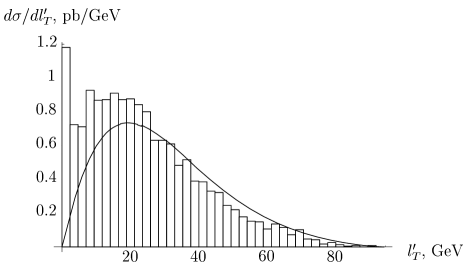
FIG. 6.: Differential cross section $d\sigma/dl^{\prime}_{T}$ versus transverse momentum of the neutrino. Our theoretical line is superimposed on results from Monte Carlo simulations using GRC4F with 3666 events.

We follow a similar procedure to obtain a graph of $d\sigma/d\eta^{\prime}$. We bin the events in pseudorapidity $\eta^{\prime}$ of the neutrino, from $\eta^{\prime}=-10$ to $\eta^{\prime}=10$, which is a reasonably large enough range to allow the cross section to fall off sharply at its edges, and we plot a histogram. Finally, we numerically integrate the differential cross section we calculated,

$$\frac{d\sigma}{d\eta^{\prime}}=\int_{0}^{l^{\prime}_{T{\mathrm{max}}}}dl_{T}^{\prime}\frac{d\sigma}{dl_{T}^{\prime}d\eta^{\prime}}.$$ (60)

From the boundary conditions of the physical region, the integration range of $l_{T}^{\prime}$ is from $0$ to $l^{\prime}_{T{\mathrm{max}}}$,

$$l^{\prime}_{T{\mathrm{max}}}=\frac{\sqrt{s}}{2\cosh\eta^{\prime}}.$$ (61)

The histogram and the theoretical curve are plotted in Fig. 7. Once again, we see that our approximate calculation and GRC4F agree except for large negative $\eta^{\prime}$, where the approximations we used break down.

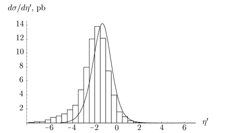
FIG. 7.: Differential cross section $d\sigma/d\eta^{\prime}$ versus pseudo-rapidity of the neutrino. Our theoretical line is superimposed on results from Monte Carlo simulations using GRC4F with 3666 events.

As a final check, we compute the total cross section $\sigma$. The GRC4F cross section is just the total number of events of this process divided by the luminosity, so $\sigma_{{\mathrm{GRC4F}}}=36.7\ {\mathrm{pb}}$. We calculate the total cross section from our result by either integrating $d\sigma/dl_{T}^{\prime}$ or $d\sigma/d\eta^{\prime}$ over their entire ranges $0<l_{T}^{\prime}<\sqrt{s}/2$ and $-\infty<\eta^{\prime}<\infty$. The cross section we obtain by either method is $\sigma_{\mathrm{th}}=30.7\ {\mathrm{pb}}$. This is in reasonable agreement with the GRC4F result.

In conclusion, we see that the cross section we calculated analytically from first principles in the leading log appromation is not far off from the GRC4F cross section in the region of large $l^{\prime}_{T}$ and not too negative $\eta^{\prime}$, where the momentum transfer from the electron is large.

VII Refinement using the GRS parton distributions

So far, our calculation has been at order $\alpha_{s}^{0}$, using pointlike parton distribution functions of quarks in a photon, without any evolution. The GRC4F result was exact at order $\alpha^{4}\alpha_{s}^{0}$, and our approximate calculation was a leading logarithm calculation at order $\alpha^{4}\alpha_{s}^{0}$. In this section, we extend the calculation to include strong interaction effects. We continue to work in the approximation that virtualities are strongly ordered (the leading log approximation) since we have seen that this approximation works well for large $l_{T}^{\prime 2}$ and $\eta^{\prime}\stackrel{{\scriptstyle>}}{{\scriptstyle\sim}}-3$. We investigate two strong interaction effects. First, the emission of gluons from the quark before it is struck can lead to contributions of order $\sum_{N}(\alpha_{s}\ln Q^{2}/|p^{2}|)^{N}$, that tend to lower the cross section. We can account for these potentially important contributions by using parton distribution functions $f_{q/\gamma}$ that have evolved according to the DGLAP evolution equation. Second, for $|p^{2}|\stackrel{{\scriptstyle<}}{{\scriptstyle\sim}}m_{\rho}^{2}$, there can be important nonperturbative hadronic contributions to $f_{q/\gamma}$. This “vector meson dominance” component can be modelled by using the parton distribution functions in pions [5], which are determined empirically. We can account for both these effects by using the recently published [3] parton distribution function for virtual photons by Glück, Reya, and Schienbein (GRS).

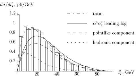
FIG. 8.: Differential cross section $d\sigma/dl_{T}^{\prime}$ versus transverse momentum of the neutrino. Our theoretical $\alpha^{4}\alpha_{s}^{0}$ leading-log calculation and the contributions due to the pointlike component of the GRS parton distribution, the hadronic component of the GRS parton distribution and the total GRS parton distribution are superimposed on $\alpha^{4}\alpha_{s}^{0}$ results from Monte Carlo simulations using GRC4F with 3666 events.

We define the virtuality of the photon to be $-p^{2}$. In the calculation that follows, we will make the approximation $p^{2}=-p_{T}^{2}$. The GRS parton distribution of a virtual photon has the form

$$f_{q/\gamma}^{\mathrm{GRS}}(x,Q^{2},-p^{2}) = f_{q/\gamma}^{\mathrm{pl}}(x,Q^{2},-p^{2})+f_{q/\gamma}^{\mathrm{had}}(x,Q^{2},-p^{2})$$ (62)

$$= f_{q/\gamma}^{\mathrm{pl}}(x,Q^{2},-p^{2})$$ (64)

$$+\frac{\alpha}{(1-p^{2}/m_{\rho}^{2})^{2}}\left(G_{q}^{2}f_{q/\pi}(x,Q^{2})+\delta_{q}\frac{1}{2}(G_{u}^{2}-G_{d}^{2})f_{s/\pi}(x,Q^{2})\right),$$

with $G_{u}^{2}\simeq 0.836$, $G_{d}^{2}\simeq 0.250$, and $\delta_{u}=-1$, $\delta_{d}=+1$. The two pieces of this parton distribution are the pointlike piece $f_{q/\gamma}^{\mathrm{pl}}$ and the hadronic piece $f_{q/\gamma}^{\mathrm{had}}$. The latter is a function of the parton distribution in a pion $f_{q/\pi}$ and of the strange sea distribution $f_{s/\pi}$, weighted by factors of order unity and a overall factor $(1-p^{2}/m_{\rho}^{2})^{-2}$ which turns on sharply as the virtuality $-p^{2}$ of the photon goes below the mass squared, $m_{\rho}^{2}$, of the $\rho$ meson. Here $\pi$ refers to the neutral pion $\pi^{0}$. The nonperturbative hadronic part is seen to start playing a role in the overall parton distribution at low photon virtuality, where the photon can be naïvely thought of as a vector meson. The distributions $f_{q/\gamma}^{\mathrm{pl}}$, $f_{q/\pi}$ and $f_{s/\pi}$ are specified parametrically by Glück, Reya, and Schienbein. We compute the distribution of quarks in an electron using the convolution

$$f_{q/e}^{\mathrm{GRS}}(x,Q^{2}) = \frac{\alpha}{2\pi}\int_{x}^{1}\frac{d\xi}{\xi}\int_{m_{e}^{2}}^{M^{2}}\frac{dp_{T}^{2}}{p_{T}^{2}}P_{\gamma/e}(x/\xi)f_{q/\gamma}^{\mathrm{GRS}}(\xi,Q^{2},p_{T}^{2}).$$ (65)

We perform the calculations of the differential cross sections as described earlier, using the new GRS distributions. The results are displayed in Figs. 8 and 9.

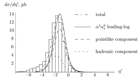
FIG. 9.: Differential cross section $d\sigma/d\eta^{\prime}$ versus pseudo-rapidity of the neutrino. Our theoretical $\alpha^{4}\alpha_{s}^{0}$ leading-log calculation and the contributions due to the pointlike component of the GRS parton distribution, the hadronic component of the GRS parton distribution and the total GRS parton distribution are superimposed on $\alpha^{4}\alpha_{s}^{0}$ results from Monte Carlo simulations using GRC4F with 3666 events.

We notice a few interesting features of the differential cross sections calculated using the GRS distributions. The cross section due to the pointlike GRS distribution has the general shape of the cross section we calculated using our unevolved pointlike distribution but is somewhat smaller. We should mention that the lower cut-off on $k_{T}$, $k_{T}^{2}>\max((0.28\ \mathrm{GeV})^{2},p_{T}^{2})$, we use to match the GRC4F results is lower than the corresponding cut-off used by GRS, $\max(0.26\ \mathrm{GeV^{2}},p_{T}^{2})$. If we set our cut-off equal to the GRS cut-off, the difference between our unevolved pointlike distribution and the GRS pointlike distribution diminishes, but does not vanish. One conjectures that this difference is due to the evolution built into the parametrization of the GRS pointlike distribution. The contribution due to the hadronic piece of the GRS distribution is fairly soft, as one would expect. The differential cross sections $d\sigma/dl_{T}^{\prime}$ (Fig. 8) and $d\sigma/d\eta^{\prime}$ (Fig. 9) are in reasonably close agreement with the GRC4F Monte-Carlo data, except once again at low $l_{T}^{\prime}$ and very negative $\eta^{\prime}$.

This check of our calculation and of the GRC4F Monte-Carlo leads us to believe that the exact result of the differential cross sections should lie reasonably close to the total GRS curves in Fig. 8 and 9, excluding perhaps the very low $l_{T}^{\prime}$ and very negative $\eta^{\prime}$ regions. One estimate of the error would be the difference between the GRS curves and the $\alpha_{s}^{0}\alpha_{s}^{4}$ leading-log curves.

We conclude that the GRC4F data is for the most part within the errors of our calculation. This gives us confidence both in our calculations and the GRC4F Monte Carlo. Finally, we have gained some insight into the physical content of the different parts of the cross section.

REFERENCES

[1] OPAL Collaboration, G. Abbiendi et al., Eur. Phys. J. C 14, 73 (2000).
[2] J. Fujimoto et al.,
Comput. Phys. Commun. 100, 128 (1997).
[3] M. Glück, E. Reya and I. Schienbein, Phys. Rev. D
60, 054019 (1999); Erratum Phys. Rev. D 62, 019902(E) (2000).
[4] J. B. Kogut and D. E. Soper, Phys. Rev. D 1, 2901 (1970); J. D. Bjorken, J. B. Kogut and D. E. Soper, Phys. Rev. D 3, 1382 (1971).
[5] M. Glück, E. Reya and I. Schienbein, Eur. Phys. J. C 10, 313 (1999).