Correlations of Solar Neutrino Observables for SNO

Neutrino oscillation scenarios predict correlations, and zones of avoidance, among measurable quantities such as spectral energy distortions, total fluxes, time dependences, and flavor content. The comparison of observed and predicted correlations will enhance the diagnostic power of solar neutrino experiments. A general test of all presently-allowed (2$\nu$) oscillation solutions is that future measurements must yield values outside the predicted zones of avoidance. To illustrate the discriminatory power of the simultaneous analysis of multiple observables, we map currently allowed regions of $\Delta m^{2}-\sin^{2}2\theta$ onto planes of quantities measurable with the Sudbury Neutrino Observatory (SNO). We calculate the correlations that are predicted by vacuum and MSW (active and sterile) neutrino oscillation solutions that are globally consistent with all available neutrino data. We derive approximate analytic expressions for the dependence of individual observables and specific correlations upon neutrino oscillations parameters. We also discuss the prospects for identifying the correct oscillation solution using multiple SNO observables.

I Introduction

After more than three decades of study, the number of proposed particle physics solutions to the solar neutrino problem is still increasing with time. The currently viable solutions to the available set of experimental data include two, three, and four neutrino oscillation scenarios (with vacuum and MSW oscillations among active as well as sterile neutrinos), neutrino decay, violation of Lorentz invariance, violation of the weak equivalence principle, and magnetic-moment transitions. Even for the simplest case of two neutrino oscillations, there are several isolated regions in neutrino parameter space that are consistent with all of the published data by the chlorine, Kamiokande, SuperKamiokande, GALLEX, and SAGE experiments.

The existing solar neutrino data provide at most (2–3)$\sigma$ indications favoring specific solutions. Moreover, the predicted sizes of those neutrino conversion effects that do not depend upon the standard solar model and that can be measured well in the Sudbury Neutrino Observatory (SNO) [1], are typically small: from a few per cent to about ten per cent [2]. Exceptions include the day-night asymmetry (for limited values of the oscillation parameters) and the double ratio of the neutral- to charged-current event rates. We will have to be lucky for the oscillation effects to be realized near their maximal possible values. In the largest part of the $\Delta m^{2}-\sin^{2}2\theta$ parameter space, currently acceptable neutrino oscillation scenarios predict that most of the new physics effects for SNO will typically be less than $3$ or $4$ $\sigma$ different from the no-oscillation predictions. And, as previous experience teaches us, Nature seems to prefer toying with us by providing ambiguous hints. The existence of systematic effects at the several percent level further increases the difficulty of identifying a unique solution.

In this paper, we show how the predictions for some solar neutrino observables are correlated, or why they are uncorrelated, in the context of specific solutions of the solar neutrino problems. We demonstrate that the signatures of a given neutrino solution include not only the values of specific observables, but also the correlations among the observables. A study of the correlations (and, where relevant, the lack of correlations) between the different predicted values of neutrino observables can be used to increase our understanding of the physical processes that are occurring.

In addition, there are excluded regions that we call “zones of avoidance.” None of the currently favored oscillation solutions predict that the measured neutrino observables will lie within these regions of avoided parameter space. We stress the diagnostic value of testing predictions that new measurable quantities lie outside these current zones of avoidance.

The main point of this paper is that studying the predicted correlations and zones of avoidance among solar neutrino observables can add discriminatory power to solar neutrino experiments. Although we illustrate the methodology using SNO variables and a particular set of allowed neutrino oscillation parameters, the diagnostic value of the predicted correlations and zones of avoidance are more general than the particulars of our illustrative calculations.

A Previous discussions of correlations

Correlations of solar neutrino observables have been discussed in several previous investigations. Perhaps the first such discussion pointed out (Ref. [3]) the lack of consistency, if no new physics were involved, between the total rates observed in the chlorine [4] and in the Kamiokande [5] experiments. This inconsistency was used as an argument to exclude astrophysical solutions of the solar neutrino problem. Kwong and Rosen (Ref. [6]) analyzed the relations between event rates measured with SuperKamiokande and with the Sudbury Neutrino Observatory (SNO) for various MSW solutions. Even more closely related to what we discuss in the present paper, Folgi, Lisi, and Montanino [7] mapped the Large Mixing Angle (LMA) MSW and the Small Mixing Angle (SMA) MSW solution regions in the $\Delta m^{2}-\sin^{2}2\theta$ plane onto the plane of flux independent observables: the day-night asymmetry, and the shift of the first moment of the electron spectrum measured with SuperKamiokande and SNO. The goal of the Bari group [7] was to show how correlations could be used to help distinguish between the SMA and the LMA solutions. The correlations of a spectrum distortion and the day-night asymmetry for SMA and MSW Sterile solutions were discussed in Ref. [8].

As discussed in Ref. [9], strong correlation exists between the day-night asymmetry and the seasonal variations of signals for the MSW solutions: both effects originate from the same earth regeneration effect. For the SMA solution, a strong correlation exists between the total day-night asymmetry and the event rate in the ”core bin” (the night bin in which neutrinos cross the core of the earth) [10]. For vacuum oscillation solutions (VAC) it has been pointed out in Ref. [11] that there is a strong correlation of spectrum distortion and seasonal variations.

In Ref. [2], we described the goal of analyzing simultaneously all of the SNO observables, measured and upper limits, in order to best constrain the allowed neutrino solutions. As a first step in that direction, we considered some pairs of measurable quantities but did not calculate the correlations between the predictions in the planes formed by the observables.

In this paper, we illustrate the power of studying the correlations between different solar neutrino observables by evaluating the correlations between measurable quantities in the SNO experiment. We elucidate the physical basis for the correlations with the aid of simple analytic approximations.

B Correlated SNO Observables

We consider here the correlations between the following quantities that are measurable in the SNO experiment.

• The total reduced rate of the charged-current events above a specified threshold:

  $${\rm[CC]}~{}\equiv~{}\frac{N_{\rm CC}}{N_{\rm CC}^{\rm SSM}}~{}.$$ (1)

  Here $N_{\rm CC}$ is the observed number of events from the CC (neutrino capture reaction by deuterium) and $N_{\rm CC}^{\rm SSM}$ is the number expected on the basis of the BP98 standard solar model [12] and no new particle physics beyond what is predicted by the standard electroweak model. The predictions for [CC] implied by the six currently allowed two-neutrino oscillation solutions have been calculated in [13] and are also discussed in [2].

  In what follows, we consider first the correlations of different experimental quantities with [CC] since the CC rate is the easiest quantity for the SNO collaboration to measure.

• The day-night asymmetry of the charged-current events [14]:

  $$A_{{\rm N-D}}^{\rm CC}~{}\equiv~{}2\frac{{\rm N}-{\rm D}}{{\rm N}+{\rm D}}~{}.$$ (2)

  Here N and D are the rates of the events observed during the night-time (N) and the day-time (D) averaged over the year (and corrected for the seasonally changing distance between the sun and the earth). The contours of constant $A_{\rm N-D}^{\rm CC}$ have been calculated in Ref. [15]. In what follows, we will use the notation $A_{\rm N-D}$ to denote the charged-current day-night effect and will use the more cumbersome notation, $A_{\rm N-D}^{\rm CC}$, only when there is a chance of confusion with the day-night effect measured from neutrino-electron scattering in SuperKamiokande, $A_{\rm N-D}^{\rm ES}$.

• The relative shift of the first moment of the electron energy spectrum from its non-oscillation value :

  $$\delta T\equiv\frac{T-T_{0}}{T_{0}}~{}.$$ (3)

  Here $T$ and $T_{0}$ are the first moments of the recoil electron energy distribution calculated with and without neutrino oscillations. The shift has been defined in [16]; we calculated $\delta T$ in Ref. [2] for the currently allowed set of neutrino parameters. The distortion is expected to be smooth for all solutions except for vacuum oscillations with large $\Delta m^{2}$, so that the first moment characterizes the distortion of the recoil energy spectrum rather well.

• The double ratio of the reduced neutral-current rate (neutrino disintegration of deuterium), $N_{\rm NC}$, to the reduced charged-current event rate:

  $$\frac{\rm[NC]}{\rm[CC]}~{}\equiv~{}\frac{N_{\rm NC}/N_{\rm CC}}{(N_{\rm NC}/N_{\rm CC})^{\rm SSM}}~{}.$$ (4)

  We will also discuss the ratio of the reduced rates of neutrino-electron scattering [ES] and charged current events [CC]: [ES]/[CC],

  $$\frac{\rm[ES]}{\rm[CC]}~{}\equiv~{}\frac{N_{\rm ES}/N_{\rm CC}}{(N_{\rm ES}/N_{\rm CC})^{\rm SSM}}~{}.$$ (5)

  Here [ES] $\equiv N_{\rm ES}/N_{\rm ES}^{\rm SSM}$, where $N_{\rm ES}$ is the number of observed $\nu-e$ scattering events and $N_{\rm ES}^{\rm SSM}$ is the number of predicted events according to the SSM.

Additional SNO observables are discussed in [2]. In particular, the seasonal variations may be significant for both vacuum[17] and MSW[2, 18] solutions.

C Outline of this paper

In Sec. II, we describe our method. In the next three sections, we study correlations related to the charged-current (CC) events observable with SNO: $A_{\rm N-D}-$ [CC] in Sec. III, [CC] - $\delta T$ in Sec. IV, and $A_{\rm N-D}-\delta T$ in Sec. V. We discuss in Sec. VI correlations in the plane of [NC]/[CC] and $A_{\rm N-D}$ and in Sec. VII the correlations of [NC]/[CC] and $\delta$T. In Sec. VIII, we summarize our results. In the Appendix, we describe the dependence on oscillation parameters of each of the observables discussed in the main text. Simple analytic expressions for these dependences are presented in the Appendix; these analytic expressions are useful for interpreting the results of detailed numerical calculations.

D How should this paper be read?

The most efficient way to read this paper is to first obtain an overview of what is accomplished and then to descend into the details. We recommend that the reader begin by looking at Fig. 2 to Fig. 11, which show the correlations and the zones of avoidance in planes constructed from quantities that are measurable by SNO. Then we suggest that the reader turn immediately to Sec. VIII, where we provide a succinct summary of our principal results and conclusions. Only after having acquired this overview, do we recommend returning to Sec. II in order to read about the details.

II Method

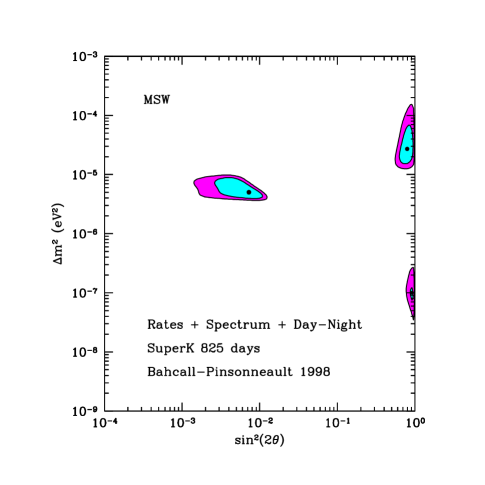
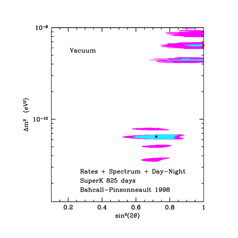
FIG. 1.: Global oscillation solutions. The input data include the total rates in the Homestake, Sage, Gallex, and SuperKamiokande experiments, as well as the electron recoil energy spectrum and the Day-Night effect measured by SuperKamiokande in 825 days of data taking. Figure 1a shows the global solutions for the allowed MSW oscillation regions, known, respectively, as the SMA, LMA, and LOW solutions [19]. Figure 1b shows the global solution for the allowed vacuum oscillation regions. The CL contours correspond, for both panels, to $\chi^{2}=\chi^{2}_{\rm min}+4.61(9.21)$, representing 90% ( 99% CL) relative to each of the best-fit solutions which are marked by dark circles.

For specificity, we consider correlations of observables in the SNO experiment for the two-flavor neutrino solutions of the solar neutrino problem. Each solution is characterized by the two oscillation parameters, $\Delta m^{2}$ and $\sin^{2}2\theta$. We use the techniques described in Ref. [19] to determine the allowed regions for the oscillation parameters. The input data used here include the total rates in the Homestake, Sage, Gallex, and SuperKamiokande experiments, as well as the electron recoil energy spectrum and the Day-Night effect measured by SuperKamiokande in $825$ days of data taking.

Fig. 1 shows the acceptable regions of the solutions in the plane of $\Delta m^{2}-\sin^{2}2\theta$ as determined in Ref. [13]. For our study of correlations, as exhibited in Fig. 2-Fig. 11, we use the $99$% C.L. solutions shown in Fig. 1.

We stress that the particular topography of the predicted correlations and the zones of avoidance depend upon the set of experimental data that are used in finding the allowed regions and the Confidence Limit (CL) that is adopted. We have adopted the input data and the CL specified above. Of course, the correlations and the zones of avoidance will evolve as more experimental data become available. Hopefully, the predicted correlations will become stronger and the zones of avoidance much larger.

We perform both numerical and semi-analytical studies of correlations. The analytic work provides, in many cases, a simple interpretation of the numerical results.

For SNO, two solar neutrino fluxes are relevant: the ⁸B flux and the $hep$ flux. We characterize these two neutrino fluxes by the dimensionless parameters $f_{B}$ and $f_{hep}$ [20, 21], which are the fluxes in units of the BP98 Standard Solar Model fluxes [12].

A Mapping from neutrino space to observable space

Predicted values of SNO observables, $X$ (e.g., [CC], $A_{\rm N-D}$, $\delta T$, [NC]/[CC]), are functions of two oscillation parameters and two flux parameters:

$$X\equiv X(\Delta m^{2},\sin^{2}2\theta,f_{B},f_{hep}).$$ (6)

Following the same procedure as in Ref. [13], we determine $f_{B}$ and $f_{hep}$ for each pair of values of the oscillation parameters, $\Delta m^{2}$ and $\sin^{2}2\theta$, by fitting to the total rate and the recoil electron energy spectrum of SuperKamiokande [22]:

$$f_{B}=f_{B}(\Delta m^{2},\sin^{2}2\theta),~{}~{}~{}~{}f_{hep}=f_{hep}(\Delta m^{2},\sin^{2}2\theta).$$ (7)

After this determination, the SNO observables are functions of two oscillation parameters only:

$$X=X(\Delta m^{2},~{}\sin^{2}2\theta).$$ (8)

The correlations depend on the form of the functions, Eq. (8); the functions are different for each solution of the solar neutrino problem. We give in the Appendix simple parametrizations of the dependences for various oscillation solutions.

In what follows, we find regions in planes of ($X$, $Y$) observables allowed by the data from all existing solar neutrino experiments. Formally, this is equivalent to mapping the solution regions in the $\Delta m^{2}-\sin^{2}2\theta$ plane onto the plane of observables of $X$ - $Y$. For each point $\Delta m^{2}-\sin^{2}2\theta$ of the solution regions, we calculate values of $X$ and $Y$. The mapping is given by Eq. (8).

If the region of an oscillation solution in the $\Delta m^{2}-\sin^{2}2\theta$ plane is projected onto a line segment or onto a narrow strip in the $X$ and $Y$ space, then we say that there is a strong correlation of the observables $X$ and $Y$ for the specified solution. In some cases, there is a strong correlation only in part of a given solution region.

There are various ways one might quantify the degree of correlation. The most appropriate way for our purpose (enhancing the identification power of the analysis) is the following. Let us denote by $S_{XY}$ the area of the region in the $X-Y$ plane to which a given solution region is projected. Let $\Delta X$ and $\Delta Y$ be the intervals of the observables $X$ and $Y$ in which these observables can vary within a given solution region if we consider the variables as independent. The product $\Delta X\times\Delta Y$ is the area of the mapped region if $X$ and $Y$ are uncorrelated. The degree of the correlation of $X$ and $Y$ can be characterized by the ratio:

$$\kappa_{XY}\equiv\frac{S_{XY}}{\Delta X\times\Delta Y}~{}.$$ (9)

If the correlation parameter $\kappa_{XY}<<1$, we will say that a strong correlation of the $X$ and $Y$ observables exists. In this case, the allowed $X$ and $Y$ parameter space is small and “zones of avoidance” dominate. For strong correlations, a combined study of the observables $X$ and $Y$ will enhance the identification power of the analysis. If $\kappa_{XY}\sim 1$, there is no correlation and no advantage to a combined study of $X$ and $Y$.

B Analytic approximations

The accurate prediction of solar neutrino observables requires multiple integrations over energy-dependent survival probabilities and neutrino interaction cross sections, and also over the energy resolution and the efficiency of detection. In spite of the complicated nature of the accurate calculations, simple and useful analytic results can often be found. The analytic expressions generally contain a small number of parameters that can be determined using the detailed numerical results. In developing analytic approximations, we proceed as described below.

First, we determine the functional dependence of the observables on the neutrino oscillation parameters, primarily through the dependence of the survival probability, $P$, on the oscillation parameters. Thus

$$X(\Delta m^{2},\sin^{2}2\theta)~{}\sim~{}X(P(\Delta m^{2},\sin^{2}2\theta))~{},$$ (10)

where the parameter $P$ represents the survival probability after a suitable average over the energy. Therefore the first step is to find expressions for observables in terms of $P$.

Second, the expressions for the survival probability $P$ can usually be simplified in the restricted regions of oscillation parameters that apply to specific allowed solutions. Also, averaging over relatively small intervals of energies (smoothing the dependences) often leads to further simplification.

Third, in the analytic expressions for observables, the average neutrino energy should be taken as a fitting parameter, which is determined by comparison of the analytic expression with the detailed results of numerical calculations. The energy parameter should be fitted separately for different solutions and for different observables. Moreover, if a given observable is described by several terms with different dependences on energy, the characteristic energy in each term should be considered as an independent parameter. This procedure will usually give the correct parametrization provided that there are no particularly strong energy dependences. The approximation generally works well if the fractional change of the survival probability over the effective range of integration is reasonably small. This condition is usually satisfied for most SNO observables.

In some cases, e.g., when observables depend on the same combination of oscillation parameters, the exact results for correlations can be obtained without performing complicated integrations over energies and over instrumental characteristics.

In summary, we find dependences of observables on oscillation parameters in terms of simple functions with a few fitting parameters that are determined by exact numerical calculations. The fitting parameters represent the complicated results of integrations over energies and over instrumental characteristics.

C Survival probabilities, observables, and correlations

We find in this subsection the dependence of different neutrino observables on the average survival probability. This is the first step in the process of deriving analytic expressions for correlations, which was outlined in the previous subsection. We shall see that some correlations appear clearly even when only survival probabilities are considered. In the Appendix, we derive expressions for the survival probabilities and show how these expressions can be used to predict correlations among neutrino observables.

1 Charged current in SNO and neutrino-electron scattering in SuperKamiokande

The reduced CC-event rate in the SNO detector can be written as

$${\rm[CC]}~{}=~{}P_{\rm SNO}\cdot f_{B}~{},$$ (11)

where $P_{\rm SNO}=P_{\rm SNO}(\Delta m^{2},\sin^{2}2\theta,E^{th})$ is the effective survival probability for CC events in SNO experiment. The $hep$ neutrinos do not contribute significantly to the total rate for an energy threshold in the likely range of $5$ to $8$ MeV and therefore $hep$ neutrinos can usually be neglected. We determine the flux parameter $f_{B}$ from the reduced total rate of events in the SuperKamiokande neutrino-electron scattering experiment:

$${\rm[ES]}_{\rm SK}~{}\equiv~{}N_{\rm SK}/N_{\rm SK}^{\rm SSM},$$ (12)

where $N_{\rm SK}$ and $N_{\rm SK}^{\rm SSM}$ are the observed and the SSM (BP98, see Ref. [12]) predicted event rates, respectively. In the case of oscillations into active neutrinos we find

$$f_{B}~{}\approx~{}\frac{\rm[ES]_{\rm SK}}{P_{\rm SK}+(1-P_{\rm SK})r}~{},$$ (13)

where $r\approx 0.16$ [23] is the ratio of the $\nu_{\mu}-e$ to the $\nu_{e}-e$ cross-sections, and $P_{\rm SK}=P_{\rm SK}(\Delta m^{2},\sin^{2}2\theta,E^{th})$ is the effective survival probability for the SK experiment.

Thus, we find from Eq. (11) and from Eq. (13)

$${\rm[CC]}~{}\approx~{}\frac{\rm[ES]_{\rm SK}}{(1-r)(P_{\rm SK}/P_{\rm SNO})+r/P_{\rm SNO}}~{},$$ (14)

where the ratio $P_{\rm SK}/P_{\rm SNO}$ depends in general on the oscillation parameters but is often of the order of unity. Equation (14) simplifies considerably if we make the approximation (valid for example if the SK and SNO energy thresholds are chosen near the plausible values of $E_{\rm SK}^{th}\sim 6.5$ MeV and $E_{\rm SNO}^{th}\sim 5$ MeV, see Ref. [24]) that $P_{\rm SK}~{}\approx~{}P_{\rm SNO}~{}=~{}P$. In this special circumstance,

$${\rm[CC]}~{}\approx~{}\frac{\rm[ES]_{\rm SK}}{1-r+r/P}~{}.$$ (15)

Equation (15) is generally valid for the LMA and LOW solutions [9], for which the survival probability depends only weakly on the energy in the energy range of interest.

In the case of conversion to sterile neutrinos ($r\rightarrow 0$), we have

$${\rm[CC]_{\rm Sterile}}~{}=~{}{\rm[ES]}_{\rm SK}\frac{P_{\rm SNO}}{P_{\rm SK}}~{}\approx~{}{\rm[ES]}_{\rm SK}.$$ (16)

For $P_{\rm SK}~{}\approx~{}P_{\rm SNO}$, the rate [CC] is approximately equal to ${\rm[ES]}_{\rm SK}$.

Deviations from the equality $P_{\rm SK}~{}=~{}P_{\rm SNO}$ can be caused by a strong energy dependence of the survival probability, by differences in the energy dependences of the neutrino cross-sections, by difference of energy thresholds, and by differences in instrumental responses.

2 Shift of the first moment of the CC spectrum

The fractional shift of the first moment of the recoil electron energy spectrum [see Eq. (3)] is easily shown (for a negligible $hep$ flux) to be proportional to the derivative of the survival probability:

$$\delta T~{}\propto~{}\frac{E}{P}\frac{dP}{dE}~{},$$ (17)

where $P$ and $dP/dE$ are suitable spectrum averages and $E$ is a characteristic energy.

3 Day-Night asymmetry

The day-night asymmetry can be estimated from the expression

$$A_{\rm N-D}^{\rm CC}~{}=~{}2\frac{P_{\rm N}-P_{\rm D}}{P_{\rm N}+P_{\rm D}}~{},$$ (18)

where $P_{N}$ and $P_{D}$ are the day and the night survival probabilities averaged over the year after removal of the geometrical factor $R^{-2}$. We showed previously in Ref. [2] that the day-night asymmetry in the SNO CC-events, $A_{\rm N-D}^{\rm CC}$, and the asymmetry in the neutrino-electron scattering observed by SuperKamiokande and SNO, $A_{\rm N-D}^{\rm ES}$, are related by the approximate equation

$$A_{\rm N-D}^{\rm CC}~{}=~{}A_{\rm N-D}^{\rm ES}\left[1+\frac{r}{(1-r)P}\right]~{}.$$ (19)

Equation (19) shows that the CC day-night asymmetry that will be measured in the SNO experiment is predicted to be larger than the neutrino-electron scattering asymmetry measured by SuperKamiokande. For typical values of the average survival probability in the range $P=0.3-0.5$, the enhancement factor in brackets in Eq. (19) is between $1.4$ and $1.6$. The prediction given in Eq. (19) can be tested also by using SNO data alone since both $A_{\rm N-D}^{\rm CC}$ and $A_{\rm N-D}^{\rm ES}$ are measurable by SNO.

Combining Eqs. (15) and (19), we obtain a relation between the day-night asymmetry $A_{\rm N-D}^{\rm CC}$ and the reduced CC rate [CC]:

$$A_{\rm N-D}^{\rm CC}~{}=~{}\frac{A_{\rm N-D}^{\rm ES}{\rm[ES]}_{\rm SK}}{{\rm[CC]}(1-r)}~{},$$ (20)

where $A_{\rm N-D}^{\rm ES}$ depends mainly on the $\Delta m^{2}$ for the LMA and LOW solution regions (see Ref. [2]): $A_{\rm N-D}^{\rm ES}~{}=~{}A_{\rm N-D}^{\rm ES}(\Delta m^{2})$. This relation holds pointwise, i.e., for a particular choice of $\Delta m^{2}$ and $\sin^{2}2\theta$. Most of the range in the $A_{\rm N-D}^{\rm CC}$ and [CC] plane is due to the allowed range in $\Delta m^{2}$ and $\sin^{2}2\theta$, which washes out the pointwise dependence of Eq. (20) because in the LMA and LOW solution regions $A_{\rm N-D}^{\rm CC}$ depends primarily on $\Delta m^{2}$ and [CC] primarily depends upon $\sin^{2}2\theta$ (cf. Fig. 2 and Fig. 3 ).

4 The double ratio [NC]/[CC]

The double ratio [NC]/[CC] is equal to the inverse of the appropriately-averaged survival probability for the active neutrino case:

$${\rm[NC]/[CC]}~{}=~{}\frac{1}{P}~{}.$$ (21)

Both [NC]/[CC] and [CC] are determined by $P$ [see Eq. (15)]. Inserting Eq. (21) into Eq. (15), we obtain

$${\rm[CC]}\approx\frac{\rm[ES]_{\rm SK}}{1-r+r{\rm[NC]/[CC]}}~{},$$ (22)

which implies that [NC]/[CC] and [CC] are strongly correlated in our approach (in which $f_{B}$ is fixed by the measured SuperKamiokande rate). As a consequence of Eq. (22), the correlation plots are similar for [NC]/[CC] and [CC] when combined with other observables. A strong correlation exists also between the double ratios [ES]/[CC] and [NC]/[CC], both of which will be measured by SNO:

$$\frac{\rm[ES]}{\rm[CC]}=1-r+r\frac{\rm[NC]}{\rm[CC]}~{}.$$ (23)

For sterile neutrinos,

$${\rm[NC]/[CC]}_{\rm Sterile}~{}=~{}\frac{P^{\prime}}{P}~{}\approx~{}1~{},$$ (24)

where $P^{\prime}$ is the average survival probability for the NC event sample. Since the thresholds for NC events ($2.2$ MeV) and for CC events (expected to be greater than $5$ MeV) are different, the ratio of the average survival probabilities, $P^{\prime}/P$, is in general different from one. However, for both NC and CC events the cross section increases with neutrino energy and most of the events that are observed correspond to neutrinos with relatively high energies. For these higher energy neutrinos, the survival probability depends rather weakly on energy (see Fig. 1 of Ref. [2]). So, while $P^{\prime}/P$ is not identical to one it is in general quite close to one for practical cases.

Combining Eq. (19) and Eq. (21), we find

$${\rm[NC]/[CC]}~{}=~{}\left(\frac{1-r}{r}\right)\Biggl{[}{{A_{\rm N-D}^{\rm CC}-A_{\rm N-D}^{\rm ES}}\over{A_{\rm N-D}^{\rm ES}}}\Biggr{]}~{}.$$ (25)

Equation (25) is an example of a correlation between three observables. The equality given in Eq. (25) does not depend explicitly on the oscillation parameters and holds approximately for all three MSW active neutrino solutions. The principal inaccuracy introduced in the derivation of Eq. (25) is caused by the fact that the average survival probability, $P$, that appears in Eq. (19) is not exactly equal to the average survival probability that appears in Eq. (21).

If we neglect the dependence of the measured quantities upon energy threshold and upon the energy dependence of the rates, then the neutrino observables depend only on two parameters, $\Delta m^{2}$ and $\sin^{2}2\theta$ . Therefore any three observables $X,Y,Z$ must be correlated, except for special cases in which one or more of the observables do not depend on the oscillation parameters. Indeed, expressing the oscillation parameters in terms of the two observables, say $X$ and $Y$, we can get the relation $Z=Z(\Delta m^{2},\sin^{2}2\theta)=Z(X,Y)$. The experimental study of the validity of Eq. (25), and other similar “triple” relations, will provide important tests of the consistency of the oscillation solutions and the experimental results. Deviations from the “triple” relations that could not be explained by expected energy dependences of the experimental quantities, or by differences in the average values of $P$ for the various measurables, would indicate either the participation of more than two neutrinos in solar neutrino oscillations or a lack of consistency of the experimental results.

5 What’s next?

The functional dependence of the survival probability on the oscillation parameters depends on which particular solution of the solar neutrino problems is chosen. In the Appendix, we give the function dependences for different currently-favored oscillation scenarios. Using the expressions for $P$ given in the Appendix and the relations presented in Eq. (15), Eq. (17), Eq. (18), and Eq. (21), we derive the dependences of the SNO observables on the neutrino oscillation parameters.

In the next three sections, we present maps of neutrino oscillation solution regions onto planes constructed from different pairs of SNO observables. We discuss results for the following currently-favored two-neutrino solutions which explain all of the available solar neutrino data: Large Mixing Angle (LMA) MSW solution, Small Mixing Angle (SMA) MSW solution, Low $\Delta m^{2}$ (LOW) solution, and MSW Sterile solution based on small mixing angle MSW conversion to sterile neutrinos. There are several disconnected regions (“islands”) of the Vacuum Oscillation solutions. We will divide them into two groups: vacuum oscillation solutions with small $\Delta m^{2}$ ($\Delta m^{2}<10^{-10}$ eV²), VAC_S, and several islands with large $\Delta m^{2}$ ($\Delta m^{2}>10^{-10}$ eV²) solutions, VAC_L. For VAC_S, there are currently four allowed islands in the $\Delta m^{2}$ and $\sin^{2}2\theta$ plane. The VAC_S solutions correspond to four almost fixed values of $\Delta m^{2}$ and varying $\sin^{2}2\theta$.

III CC-rate versus Day-Night Asymmetry

Figures 2 and 3 show maps of the currently-allowed regions in the $\Delta m^{2}-\sin^{2}2\theta$ plane onto the ${\rm[CC]}-A_{\rm N-D}$ plane for the electron energy thresholds of 5 MeV and 8 MeV, respectively. In Fig. 2, we show a simulated data point near the best-fit value for the LMA solution. The estimated $1\sigma$ error bar for the CC measurement is taken from Table II of Ref. [2]. For $A_{\rm N-D}$, we assume for purposes of illustration a $\pm 0.03$ uncertainty in the absolute value as a $1\sigma$ error, which is comparable with the accuracy that has been achieved after three years with the SuperKamiokande detector [22].

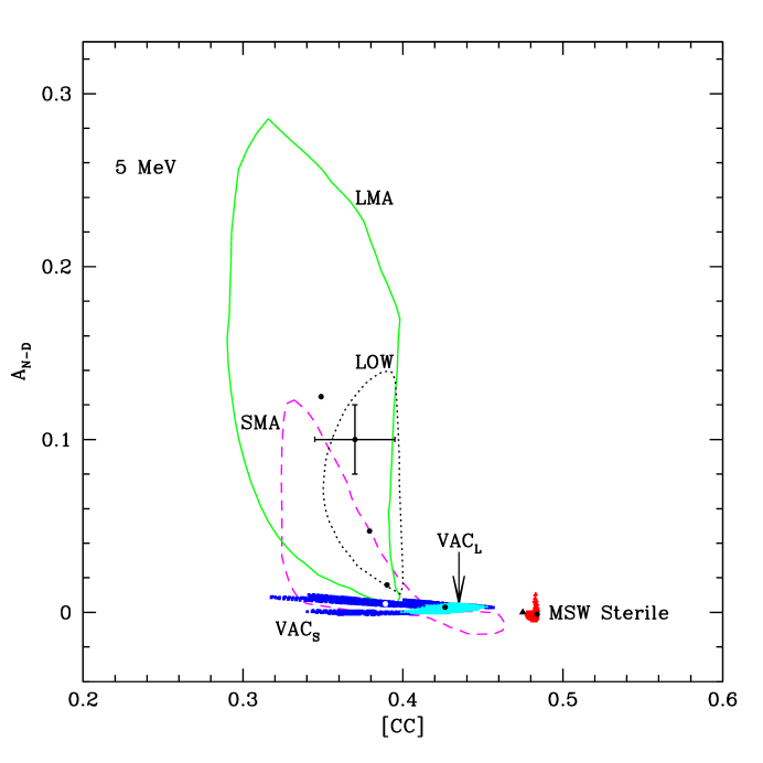
FIG. 2.: The allowed regions for the day-night asymmetry in the charged current event rate, $A_{\rm N-D}$, versus the reduced charged current rate, [CC], for an electron energy threshold 5 MeV. The figure shows the currently-allowed regions predicted by two-neutrino solutions [13] that describe all the available solar neutrino data: LMA (encircled by a solid line), SMA (dashed line), LOW (dotted line), VAC_S (black points), and VAC_L (grey points). The best-fit points for each solution are indicated by a small black circles within the allowed region. The prediction for the no-oscillations case is indicated by a triangle. The cross near the best-fit point of the LMA solution is a simulated measurement with estimated $1\sigma$ error bars.

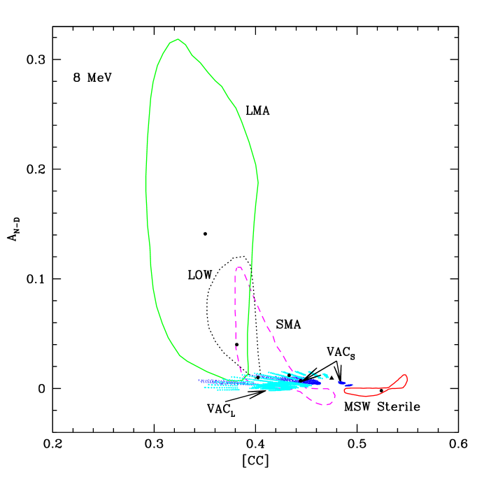
FIG. 3.: The allowed regions for the day-night asymmetry, $A_{\rm N-D}$, versus the reduced charged current rate, [CC], for an electron energy threshold $8$ MeV. The meaning of the symbols is the same as for Fig. 2, except that the regions now refer to a recoil electron energy threshold of 8 MeV.

A Discriminating among solutions

There are four regions in Fig. 2 and Fig. 3 for which (after taking account of the likely measurement uncertainties and the overlap of the predicted values of the observables) important scientific inferences will be possible if the measured values of [CC] and $A_{\rm N-D}$ fall within the designated areas. 1) If measurements show that $A_{\rm N-D}>0.2$, then that will be a strong indication in favor of the LMA solution. 2) If the measurements only show that $A_{\rm N-D}>0.1$, that by itself will be sufficient to disfavor the vacuum and MSW Sterile solutions. 3) If instead $A_{D-N}\sim 0$ and [CC] is consistent with $0.48$, then that would strongly favor the MSW Sterile solution. 4) If the measured values lie within the ‘zone of avoidance’ of $A_{\rm N-D}>0.02$ and ${\rm[CC]}>0.4$, then none of the currently acceptable oscillation solutions will be favored.

If $A_{\rm N-D}>0.1$, then the inferences from cases 1) and 2) above can be tested by measuring $\delta T$. Figure 4 and Fig. 5, as well as Fig. 6 and Fig. 7, show that all the currently allowed oscillation solutions predict $\delta T<0.01$ if $A_{\rm N-D}>0.15$.

If the day-night asymmetry lies in the broad range $0<A_{\rm N-D}<0.15$, it will be difficult to disentangle the LMA, LOW and SMA solutions. These three MSW solutions show a large overlap in their predictions for the [CC]-$A_{\rm N-D}$ plane (see Fig. 2 and Fig. 3 and especially Table IX of Ref. [2]). If the observed asymmetry is not too small, e.g., if $A_{\rm N-D}>0.1$, then the SMA solution can be identified by the zenith angle dependence of the rate during the night. According to the SMA scenario, the rate should be strongly enhanced in the deepest night bin (for the core-crossing neutrino trajectories) [25]. In contrast, the LMA and LOW solutions predict rather flat zenith angle distributions. The LOW and the LMA solutions may be distinguishable through the observed dependence of the day-night asymmetry on the energy threshold. The asymmetry increases with threshold for the LMA solution and decreases with threshold for the LOW solution. For the LMA solution, the maximal possible asymmetry becomes as large as 0.32 for $E^{th}=8$ MeV instead of 0.28 for $E=5$ MeV (see Fig. 2 and Fig. 3). For the LOW solution, the dependence upon the threshold energy is just the opposite; the predicted asymmetry decreases with increasing threshold energy. In particular, the LOW solution predicts that the maximal asymmetry decreases from $0.135$ to $0.11$ as the threshold energy increases from $5$ MeV to $8$ MeV. The LOW solution may also be identified later by strong Day-Night variations of the beryllium line in BOREXINO experiment [26].

The charged-current event ratio is in some ways the simplest experimental quantity to measure with the Sudbury Neutrino Observatory. However, the most remarkable aspect of the above analysis of Fig. 2 and Fig. 3 is that the potentially important inferences are almost entirely independent of the measured charged-current rate. This is because the estimated $1\sigma$ uncertainty in the value of [CC] is about $6.7$% (see Ref. [2]) and is dominated by the theoretical uncertainty in the charged-current neutrino-absorption cross section. Unless a major improvement is made in the accuracy of the theoretical cross section calculation, the potential diagnostic value of the charged-current measurement will be severely compromised by the large uncertainty in the neutrino absorption cross section.

B Correlation phenomenology

For the LMA solution, there is no significant correlation shown in Fig. 2 and Fig. 3; the correlation parameter, cf. Eq. (9), $\kappa_{A-CC}({\rm LMA})\sim 1$. For the largest area of the plane of oscillation parameters, the charged-current rate depends mainly on $\sin^{2}2\theta$ [see Eq. (A8)], whereas $A_{\rm N-D}$ depends strongly on $\Delta m^{2}$ [see Eq. (A10)]. There is a tendency for small values of [CC] to correspond to large values of $A_{\rm N-D}$, since [according to Eq. (20)] for fixed $\Delta m^{2}$ the asymmetry is inversely proportional to [CC].

Also for the LOW solution, no significant correlation appears. The area occupied in the [CC]-$A_{\rm N-D}$ plane by the LOW solution is substantially smaller than for the LMA solution, which reflects the smaller allowed region of the LOW solution in the $\Delta m^{2}-\sin^{2}2\theta$ plane.

The SMA solution has the form of two beautiful, asymmetric petals connected at the point of zero asymmetry. This form can be understood from the expression for the asymmetry, Eq. (A14). The zero asymmetry contour is determined by the condition $P=1/2$. Therefore, the contours of $A_{\rm N-D}=0$ and of ${\rm[CC]}=0.41$, both of which correspond to $P=1/2$, coincide. The contours are defined by the relation

$$\xi\equiv\Delta m^{2}\cdot\sin^{2}2\theta={\rm constant}~{}.$$ (26)

The correlation between $A_{\rm N-D}$ and [CC] appears in the region of small asymmetries and of large [CC]. The rate [CC] decreases with increase of $A_{\rm N-D}$ (Here $\kappa_{A-CC}({\rm SMA})\ll 1$ ) .

For vacuum solutions, there is a correlation between $A_{\rm N-D}$ and [CC] that is difficult to see on the scale of Fig. 2 and Fig. 3, because the day-night asymmetry is small. The residual asymmetry, which is calculated after first removing the $R^{-2}$ dependence of the total flux, is not zero, but $A_{\rm N-D}<2\%$ is predicted for all the currently-favored vacuum oscillation solutions [2]. By inspecting the figures carefully, one can see that the asymmetry $A_{\rm N-D}$ increases with decreasing [CC].

The day-night effect for vacuum oscillations is determined by geometrical factors. In the northern hemisphere, the nights are longer in the winter when the earth is closer to the sun. The earth-sun distance affects the vacuum oscillation probability and therefore the CC event rate. Combining Eq. (15), Eq. (A22), and Eq. (A24), we find

$$A_{\rm N-D}=\frac{1}{r}\left(\frac{\rm[ES]_{\rm SK}}{\rm[CC]}-1\right)\times f(\Delta m^{2})~{},$$ (27)

where

$$f(\Delta m^{2})\approx 2(\Delta m^{2}/m_{V}^{2})\cot(\Delta m^{2}/m_{V}^{2})$$ (28)

is a function of $\Delta m^{2}$ only. Since within a given currently-allowed “island” in the $\Delta m^{2}-\sin^{2}2\theta$ plane , the variation of $\Delta m^{2}$ is small, we can consider $f(\Delta m^{2})\approx{\rm constant}$. Equation (27) explains the correlation between $A_{\rm N-D}$ and [CC] that exists in Fig. 2 and Fig. 3.

IV Charged-Current Rate versus Shift of First Moment

Figures 4 and 5 show, for electron energy thresholds of $5$ MeV and $8$ MeV, maps onto the ${\rm[CC]}-\delta T$ plane of the currently-allowed regions in the $\Delta m^{2}-\sin^{2}2\theta$ plane. For illustrative purposes, Fig. 4 shows a simulated experimental point near the current best-fit predicted point for the LMA solution. The error bars are estimated $1\sigma$ uncertainties from Table II of Ref. [2], with a $1.3$% fractional uncertainty in the first moment and a $6.7$% for the charged-current rate.

A Discriminating among solutions

If the measured values of [CC] and $\delta T$ fall close to the current best-fit value of the LMA solution, then many of the currently-favored solutions will still be allowed if a $3\sigma$ level of disagreement is permitted. The difficulty in uniquely identifying solutions is primarily caused by the estimated $3\sigma$ uncertainties being comparable in many cases to the size of the predicted effects.

There are some regions of the two-dimensional parameter space, ${\rm[CC]}-\delta T$, that are relatively discriminatory. For example, in the region in which $\delta T>0.04$ and $0.3<{\rm[CC]}<0.4$, only the VAC_S and the SMA solutions are represented. The most extreme values of the [CC] parameter, e.g., [CC] $>0.5$ or [CC] $<0.3$, would indicate, respectively, the MSW Sterile solution or the LMA solution. If either of these cases is suggested by the [CC] measurement, then a comparison of the predicted and measured $\delta T$ (Fig. 4) and $A_{\rm N-D}$ (Fig. 2) will be useful checks of the validity of the identification of the solution.

Unique inferences will be possible (see Fig. 4) for extreme VAC_S solutions with a fractional shift $\delta T>4.5$% and for the MSW Sterile solution with [CC] greater than 0.48. The extreme VAC_S solution predicts a very small value for the day-night asymmetry, $A_{\rm D-N}<0.01$ (see Fig. 6).

Two zones of avoidance appear in Fig. 4 for large [CC]. None of the currently favored oscillation solutions predict $\delta T<0.01$ or $\delta T>0.04$ for [CC] $>0.45$. For an electron recoil energy threshold of $8$ MeV, we find that $\delta T<0.04$ for all the currently favored oscillation solutions (see Fig. 5). For smaller [CC], between $0.3$ and $0.4$, there is also a zone of avoidance for $\delta T>0.01$ and less than the values predicted by the SMA solution.

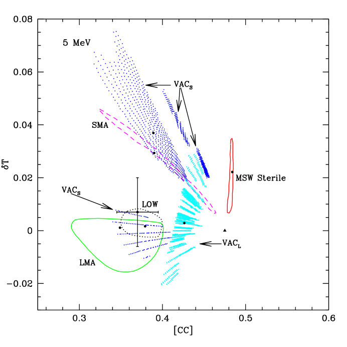
FIG. 4.: The allowed regions for the shift of the first moment, $\delta T$, versus the reduced charged current rate, [CC], for a recoil electron energy threshold of 5 MeV. The meaning of the symbols is the same as in Fig. 2, except that the regions now refer to $\delta T$ and [CC]. The nearly horizontal segments that overlap with the LOW and the LMA solution regions correspond to VAC_S solutions with the largest values of $\Delta m^{2}$.

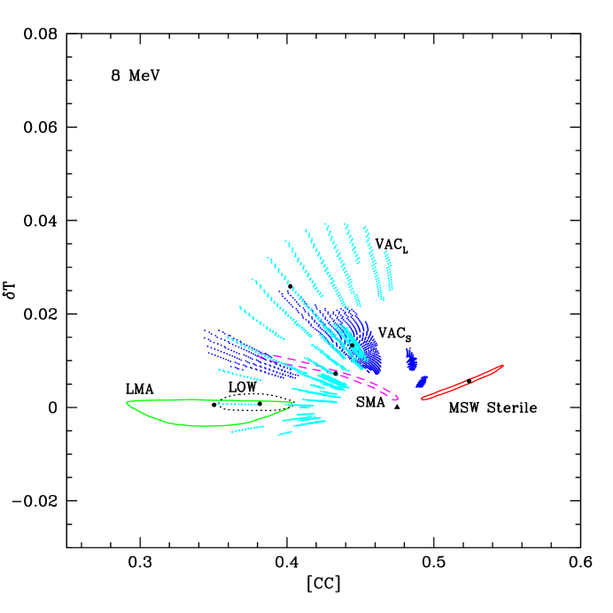
FIG. 5.: The allowed regions for the shift of the first moment, $\delta T$, versus the reduced charged current rate, [CC], for a recoil electron energy threshold of $8$ MeV. The meaning of the symbols is the same as in Fig. 2, except that the allowed regions refer to $\delta T$ and [CC] and the threshold for the recoil electron energy is $8$ MeV.

B Correlation phenomenology

For the SMA solution, both [CC] and $\delta T$ are determined by a unique combination of neutrino variables, $\xi$, defined by Eq. (26), so that (up to small earth matter effect corrections) the two measurables are strongly correlated. As $\delta T$ increases, the charged-current rate [CC] decreases (cf. Fig. 4). Using Eq. (14) (with $P_{\rm SNO}\sim P_{\rm SK}$) and Eq. (A13) for the rate and Eq. (A16) for the shift of the first moment, we find for an electron threshold energy of $5$ MeV

$${\rm[CC]}\approx\frac{\rm[ES]_{\rm SK}}{1-r+r\cdot e^{B\delta T}}~{}.$$ (29)

The numerical coefficient $B$ in the exponent that occurs in Eq. (29) is determined by results of exact numerical calculations, $B=29.3$. For an electron energy threshold of $8$ MeV, one should use the general formula given in Eq. (14) without making the approximation that $P_{\rm SNO}\sim P_{\rm SK}$.

For the VAC_S solution, a strong correlation exists. Using Eq. (15) and Eqs. (A23) and (A22), we find

$$\delta T=\frac{1}{r}\left(\frac{\rm[ES]_{\rm SK}}{\rm[CC]}-1\right)\times f(\Delta m^{2})~{},$$ (30)

where the function $f(\Delta m^{2})$, has been defined by Eq. (28). The relation given in Eq. (30) holds for each allowed island in neutrino parameter space, and, in the approximation of constant $\Delta m^{2}$, there is a strong correlation of the rate and the shift of the first moment for each of the three islands with low $\Delta m^{2}$. The first moment shift, $\delta T$, increases as [CC] decreases. For the allowed island with the largest value of $\Delta m^{2}$ (which overlaps for a $5$ MeV threshold with the LMA and LOW solutions), the shift of the first moment is close to zero and the correlations are weak.

For the MSW Sterile neutrino solution, the rate [CC] is strongly restricted by the measured value of ${\rm[ES]}_{\rm SK}$, whereas $\delta T$ varies over a significant range.

The LMA solution does not predict a strong correlation, as can easily be seen from Eqs. (A8) and (A9). The rate [CC] depends strongly on $\sin^{2}2\theta$, whereas $\delta T$ depends strongly on $\Delta m^{2}$. The situation is similar for the LOW solution.

At a higher threshold, $8$ MeV (see Fig. 5), the shift of the first moment becomes smaller for all solutions. In particular, a significant part of the LMA region with negative $\delta T$ disappears. At the same time, for the VAC_L region the best-fit point shifts to larger $\delta T$. In contrast, the spread of the [CC] rates increases especially for the SMA Sterile solution. For $E^{th}=5$ MeV, $P_{SNO}\approx P_{SK}$ and, as a consequence, [CC] is uniquely fixed by $R_{SK}$ [Eq. (16)]. For $E^{th}=8$ MeV, $P_{SNO}/P_{SK}$ differs from one and depends on oscillation parameters, which leads to the larger spread in [CC]. Also for $E^{th}=8$ MeV, the VAC_S region with the largest $\Delta m^{2}$ no longer overlaps with the LMA and the LOW solution regions.

V Shift of First Moment versus Day-Night Asymmetry

Figures 6 and 7 show maps of the currently-allowed regions in the $\Delta m^{2}-\sin^{2}2\theta$ plane onto the $\delta T-A_{\rm N-D}$ plane for the electron energy thresholds of 5 MeV and 8 MeV, respectively. In Fig. 6, the estimated $1.3$% ($1\sigma$) error bar for the $\delta T$ measurement is taken from Table II of Ref. [2]. For $A_{\rm N-D}$, we assume for purposes of illustration a $\pm 0.03$ uncertainty in the absolute value as a $1\sigma$ error, which is comparable with the accuracy that has been achieved after three years with the SuperKamiokande detector [22].

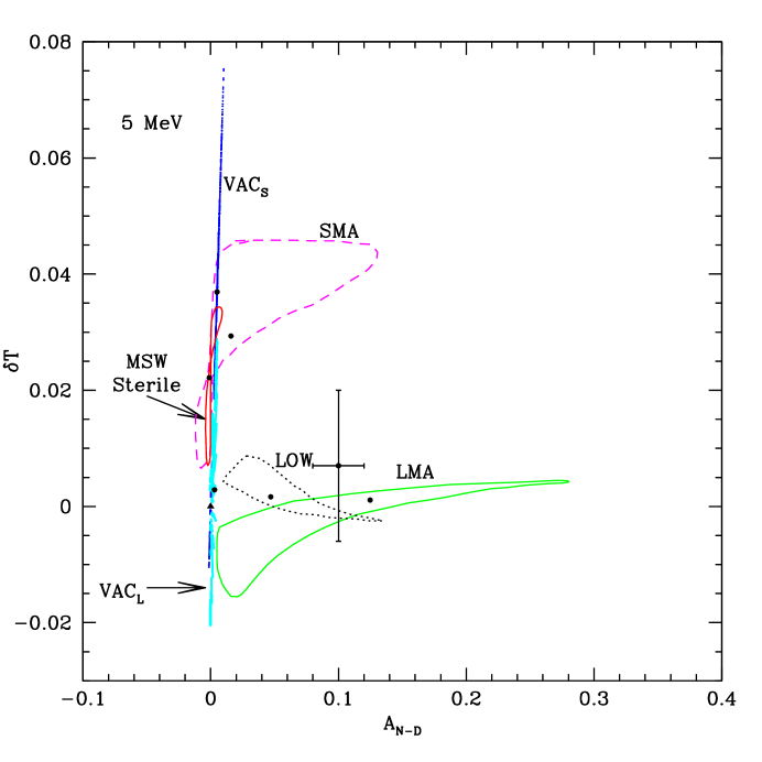
FIG. 6.: The allowed regions for the shift of the first moment, $\delta T$, versus the day-night asymmetry, $A_{\rm N-D}$, for an electron recoil electron energy threshold of $5$ MeV. The meaning of the symbols is the same as in Fig. 2, except that the allowed regions now refer to $\delta T$ and $A_{\rm N-D}$.

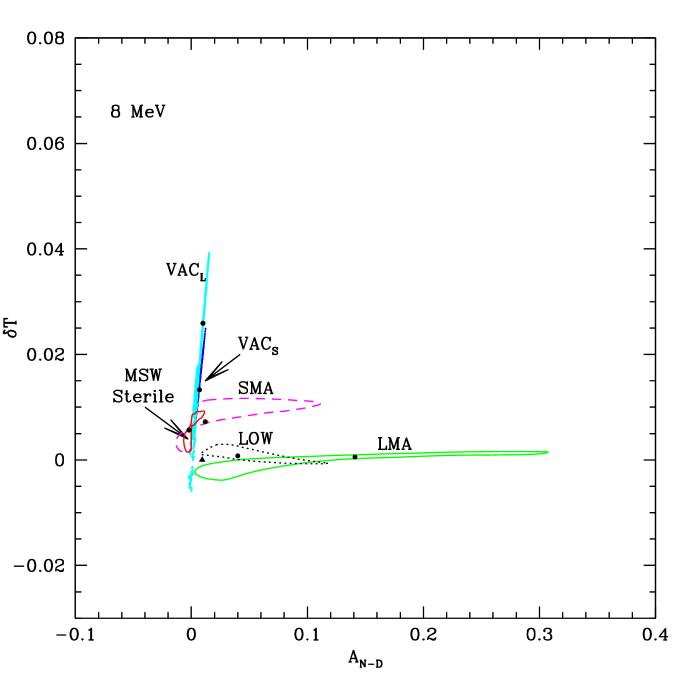
FIG. 7.: The allowed regions for the shift of the first moment, $\delta T$, versus the day-night asymmetry, $A_{\rm N-D}$, for an electron recoil electron energy threshold of $8$ MeV. The meaning of the symbols is the same as in Fig. 2, except that the allowed regions now refer to $\delta T$ and $A_{\rm N-D}$ and the threshold for the recoil electron energy is $8$ MeV.

A Discriminating among solutions

The only truly unique regions in the $A_{\rm N-D}-\delta T$ plane are the very large values of $A_{\rm N-D}>0.2$, which would favor LMA, and the very large values of $\delta T>0.06$ ($5$ MeV threshold), which would favor VAC_S. In both cases, the oscillation solution implies that the other measured parameter should be small, i.e., $\delta T$ should be small (according to LMA) if $A_{\rm N-D}$ is near its maximal value and $A_{\rm N-D}$ should be small if $\delta T$ is near its maximal value.

Both the LMA and the LOW solutions predict that the shift of the first moment is small for all allowed values of the day-night asymmetry, i.e., $-0.02<\delta T<0.015$. And, of course, the day-night asymmetry is predicted to be small for all the vacuum solutions and the MSW Sterile solution, i.e., $|A_{\rm N-D}|<0.02$ for all allowed values of $\delta T$. The imposition of these cross checks can be used to test the validity of currently-allowed oscillation solutions.

Taking into account the estimated uncertainties in the measurements, the most populated region in the $A_{\rm N-D}-\delta T$ plane contains multiple currently-allowed solutions.

It is easy to find zones of avoidance in Fig. 6 and Fig. 7. For a $5$ MeV electron recoil energy threshold, there are no predicted solutions with $A_{\rm N-D}>0.02$ and $\delta T>0.045$ nor are there any predicted solutions with $A_{\rm N-D}>0.1$ and $\delta T<0$. For an $8$ MeV energy threshold, there are no predicted solutions with $A_{\rm N-D}>0.02$ and $\delta T>0.01$.

B Correlation phenomenology

In the small $\Delta m^{2}$ limit (large day-night asymmetry), both the LMA and the LOW solutions predict an approximately linear relation between the day-night asymmetry and the fractional shift in the first moment:

$$\delta T~{}=~{}kA_{\rm N-D}~{}.$$ (31)

For the LMA solution, $k_{\rm LMA}=0.014$ and $k_{\rm LOW}=-0.03$ for a $5$ MeV threshold. These results can be obtained from Eq. (A9) and Eq. (A10) for the LMA solution and from Eq. (A20) and Eq. (A21) for the LOW solution. This weak correlation exists because in the region of small $\Delta m^{2}$ of the LMA solution and large $\Delta m^{2}$ of the LOW solution both the day-night asymmetry and the shift of the first moment are induced by the earth matter effect.

The allowed regions for the SMA and the MSW Sterile solutions both have the form of two petals connected at the point $A_{\rm N-D}=0$.

For vacuum solutions, with the accuracy that is apparent in Fig. 6 and Fig. 7, the shift of the first moment does not seem to depend significantly upon the day-night asymmetry. However, there is a linear correlation,

$$A_{\rm D-N}~{}\propto~{}\delta T,$$ (32)

where the coefficient of proportionality is sufficiently small that the variation of $A_{\rm D-N}$ about zero is not easily visible on the scale shown in the figures. The correlation arises because for vacuum oscillations $A_{\rm D-N}~{}\propto~{}RdP/dR$ and $\delta T~{}\propto~{}EdP/dE$, where the survival probability, $P$, depends upon the ratio of distance, $R$, to energy, $E$, i.e., $P=P(R/E)$ [see discussion following Eq. (A23) and Eq. (A24)]. It will be very difficult to test experimentally whether the relation given in Eq. (32) is present.

VI [NC]/[CC] versus Day-Night Asymmetry

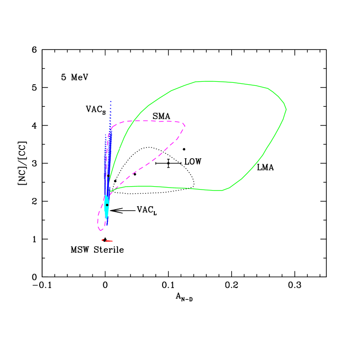
FIG. 8.: The allowed regions for the [NC]/[CC] double ratio versus the day-night asymmetry, $A_{\rm N-D}$, for a recoil electron energy threshold of $5$ MeV. The meaning of the symbols is the same as in Fig. 2, except that the allowed regions now refer to [NC]/[CC] and $A_{\rm N-D}$.

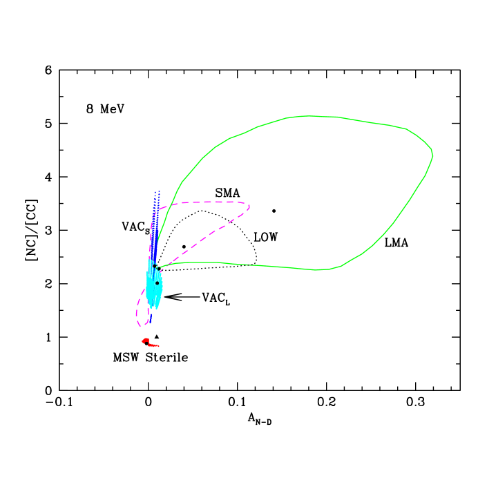
FIG. 9.: The allowed regions for the [NC]/[CC] double ratio versus the day-night asymmetry, $A_{\rm N-D}$, for a recoil electron energy threshold of $8$ MeV. The meaning of the symbols is the same as in Fig. 2, except that the allowed regions now refer to [NC]/[CC] and $A_{\rm N-D}$ and a recoil energy threshold of $8$ MeV.

Figures 8 and 9 show maps of the currently-allowed regions in the $\Delta m^{2}-\sin^{2}2\theta$ plane onto the ${\rm[NC]/[CC]}-A_{\rm N-D}$ plane for the electron energy thresholds of 5 MeV and 8 MeV, respectively. In Fig. 8, we show a simulated data point near the best-fit value for the LMA solution. The estimated $1\sigma$ error bar for the [NC]/[CC] measurement is $3.6$% after one year (Table II of Ref. [2]) and is dominated by the statistical error in the determination of the neutral-current rate. For $A_{\rm N-D}$, we assume for purposes of illustration a $\pm 0.03$ uncertainty in the absolute value as a $1\sigma$ error, comparable to the accuracy that has been achieved after three years with the SuperKamiokande detector [22].

The precision with which both the [NC]/[CC] ratio and the day-night asymmetry are measured will improve with time as more events are detected.

Figure 8 and Fig. 9 are similar to Fig. 2 and Fig. 3, because of the relation given in Eq. (22) between[NC]/[CC] and [CC]. The form of the allowed regions, the shape of the zones of avoidance, and the degree of overlap between different solutions are all quite similar in both sets of figures. But, because the double ratio [NC]/[CC] can potentially be measured with much better accuracy than [CC] alone, the correlations of [NC]/[CC] with $A_{\rm N-D}$ and other observables will have much stronger discriminatory power.

A Discriminating among solutions

There are regions in the [NC]/[CC] $-A_{\rm N-D}$ plane in which only one oscillation solution is predicted to exist and, on the other hand, regions in which there is significant overlap between different oscillation solutions. There are also significant regions, easily visible to the eye in Fig. 8 and Fig. 9, in which no oscillation solutions are predicted to lie.

We begin with a discussion of the regions where the identification of the oscillation solution may be unique and then discuss the ambiguous regions and the excluded regions.

If $A_{\rm N-D}$ is observed to be greater than $0.2$ and [NC]/[CC] is larger than $2.5$, then the LMA solution will be uniquely singled out. The measurement of the first moment of the electron recoil energy distribution will provide a check on this inference since the LMA solution implies $|\delta T|<0.01$ (see Fig. 6 and Fig. 7), i.e., a very small distortion of the charged-current energy spectrum. Moreover, the reduced [CC] rate should be consistent with a value in the range $0.3$ to $0.4$ (see Fig. 2 and Fig. 3).

If [NC]/[CC] is measured to be larger than $4.5$, then the only candidate solutions will be LMA and VAC_S. The two possibilities can be distinguished since (see Fig. 8 and Fig. 9) LMA predicts a significant day-night asymmetry, $A_{\rm N-D}>0.06$, for large [NC]/[CC] and VAC_S predicts a very small asymmetry, $|A_{\rm N-D}|<0.01$.

If, on the other hand, [NC]/[CC] is found to be smaller than $2.0$, then the LMA and LOW solutions will be eliminated. Values of [NC]/[CC] in the range $2.0$ to $1.2$ can be obtained with the SMA and vacuum solutions, but a value of [NC]/[CC] consistent with unity (and a small measurement error) would uniquely favor the MSW Sterile solution. In all cases of [NC]/[CC] less than $2.0$, the predicted day-night asymmetry is very small, $|A_{\rm N-D}|<0.02$ (see Fig. 8 and Fig. 9).

The most ambiguous region will be $2<{\rm[NC]/[CC]}<4$ and a small ($<0.02$) day-night asymmetry. Figure 8 shows that multiple oscillation solutions can give rise to observables in this region. Moderate values of $A_{\rm N-D}$ (e.g., $0.02$ to $0.12$) and moderate values of [NC]/[CC] (e.g., $2.5$ to $4.0$) will also be ambiguous since all three of the MSW active solutions, LMA, SMA, and LOW can populate this region in the ${\rm[NC]/[CC]}-A_{\rm N-D}$ plane. As we have discussed in Sec. III, a detailed study of the zenith angle distribution of the charged current events during the night may discriminate among these solutions.

The zones of avoidance in the ${\rm[NC]/[CC]}-A_{\rm N-D}$ plane are: all values of [NC]/[CC] larger than $5.2$ (for any values of $A_{\rm N-D}$, [CC], and $\delta T$): $A_{\rm N-D}$ less than $-0.02$ (for any values of [NC]/[CC], [CC], and $\delta T$); and [NC]/[CC] less than $2.5$ together with $A_{\rm N-D}$ larger than $0.02$.

B Correlation phenomenology

The correlations between [NC]/[CC] and $A_{\rm N-D}$ are similar to the correlations between [CC] and $A_{\rm N-D}$ that were discussed in Sec. III. The pointwise relation between [NC]/[CC] and $A_{\rm N-D}^{\rm CC}$ for the LMA and LOW active solutions is washed out in Fig. 8 and Fig. 9 by the fact that $A_{\rm N-D}^{\rm CC}$ depends primarily on $\Delta m^{2}$ and [NC]/[CC] primarily depends upon $\sin^{2}2\theta$.

In all cases, the day-night effect is small for vacuum oscillations. However, one can understand the general trend in Fig. 8 and Fig. 9, according to which the solutions for VAC_L (larger $\Delta m^{2}$) correspond to smaller values of [NC]/[CC] than the solutions for VAC_S.

It is easy to show from Eq. (21), Eq. (A22), and Eq. (A24) that for the VAC_S solutions

$$\frac{\rm[NC]}{\rm[CC]}=1+k\cdot A_{\rm N-D}~{},$$ (33)

where $k\equiv k(\Delta m^{2})$ is a function of $\Delta m^{2}$ only. For the VAC_S scenario, there are four islands of solutions along which $\Delta m^{2}\approx{\rm constant}$ but $\sin^{2}2\theta$ changes. So, for a given VAC_S island $k\approx{\rm constant}$, where $k$ takes on a different value for each island of solutions. From Eq. (33), we see that [NC]/[CC] increases linearly with $A_{\rm N-D}$. For $A_{\rm N-D}=0$, we obtain [NC]/[CC] $=1$. All of these features are apparent in Fig. 8 and Fig. 9.

The discussion following Eq. (24) explains why for sterile neutrinos [NC]/[CC] is predicted to be close to, but not identical to, one.

VII [NC]/[CC] versus Shift of First Moment

Figures 10 and 11 show, for electron energy thresholds of $5$ MeV and $8$ MeV, maps onto the ${\rm[NC]/[CC]}-\delta T$ plane of the currently-allowed regions in the $\Delta m^{2}-\sin^{2}2\theta$ plane. For illustrative purposes, Fig. 10 shows a simulated experimental point near the current best-fit predicted point for the LMA solution. The error bars are estimated $1\sigma$ uncertainties from Table II of Ref. [2], with a $1.3$% fractional uncertainty in the first moment and a $3.6$% for the neutral to charged-current double ratio.

Figure 10 and Fig. 11 are similar to Fig. 4 and Fig. 5; the latter pair refers to the correlation between the [CC] and the $\delta T$ variables. Because of the relation Eq. (22) between [NC]/[CC] and [CC], the acceptable solution space, as well as the zones of avoidance and the degree of overlap of the solution regions, are similar in the two sets of figures.

A Discriminating among solutions

There are certain regions of the parameter space, ${\rm[NC]/[CC]}-\delta T$, that are relatively discriminatory. For example, for a $5$ MeV threshold (see Fig. 10), in the region in which $\delta T>0.03$ and $1<{\rm[NC]/[CC]}<5$, only the VAC_S and the SMA solutions are represented. The most extreme values of the [NC]/[CC] parameter, e.g., [NC]/[CC] $>4.7$ or $<1$, would indicate, respectively, the LMA solution or the MSW Sterile solution. Only VAC_S solutions have a fractional shift $\delta T>4.5$% . Figure 10 shows significant zones of avoidance, e.g., [NC]/[CC] $>2.2$ and $0.01<\delta T<0.01{\rm[NC]/[CC]}$.

For an electron recoil energy threshold of $8$ MeV (see Fig. 11), the degree of the overlap between the predictions of different scenarios is not larger than it was for a $5$ MeV threshold, as is the case for ${\rm[CC]}-\delta T$ (cf. Fig. 4 and Fig. 5). The allowed regions of VAC_S solution with largest $\Delta m^{2}$ do not overlap with LMA and LOW regions, as occur for a $5$ MeV threshold. However, the largest $\Delta m^{2}$ VAC_S solutions do overlap with the allowed SMA region for an $8$ MeV threshold.

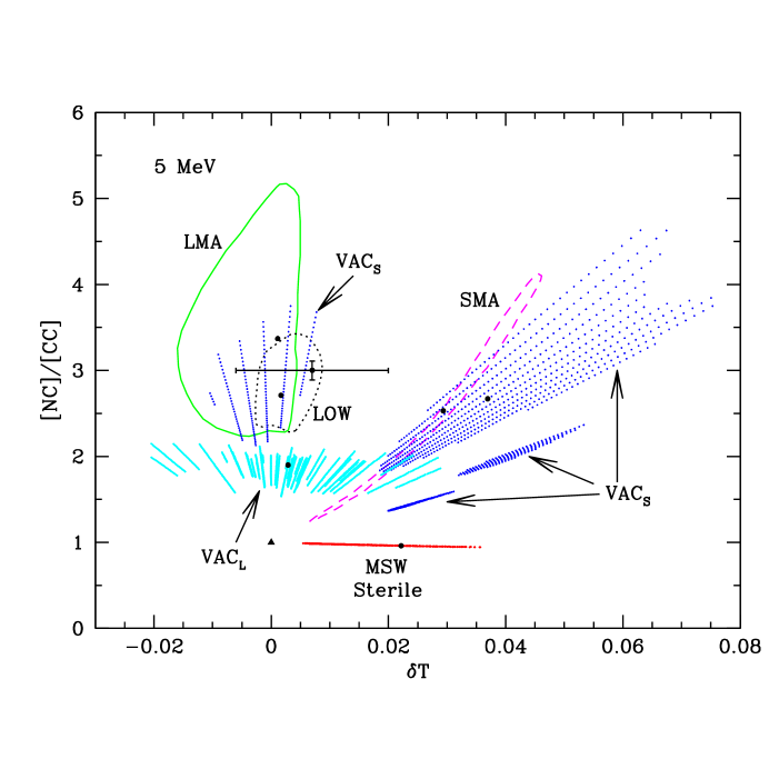
FIG. 10.: The allowed regions for the the double ratio, [NC]/[CC], versus the shift of the first moment, $\delta T$, for a recoil electron energy threshold of $8$ MeV. The meaning of the symbols is the same as in Fig. 2, except that the regions now refer to [NC]/[CC] and $\delta T$.

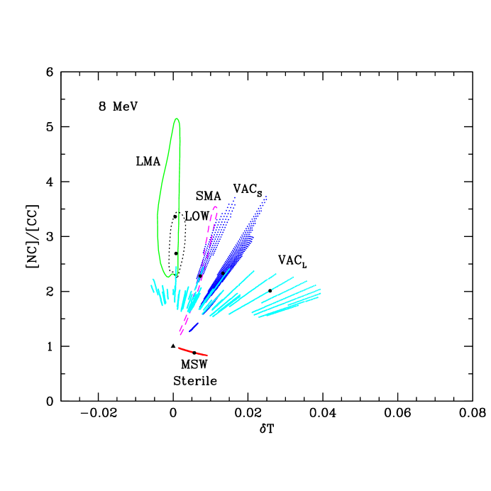
FIG. 11.: The allowed regions for the the double ratio, [NC]/[CC], versus the shift of the first moment, $\delta T$, for a recoil electron energy threshold of $8$ MeV. The meaning of the symbols is the same as in Fig. 2, except that the allowed regions refer to [NC]/[CC] and $\delta T$ and the threshold for the recoil electron energy is $8$ MeV.

B Correlation phenomenology

For the SMA solution, both [NC]/[CC] and $\delta T$ are determined by a unique combination of neutrino variables, $\xi$, defined by Eq. (26), so that the two measurables are strongly correlated: $\kappa_{\delta T-NC/CC}({\rm SMA})\ll 1$. As the shift $\delta T$ increases, the double ratio [NC]/[CC] also increases (cf. Fig. 10 and Fig. 11). Using Eq. (21) and Eq. (A12) for the survival probability and Eq. (A16) for the shift of the first moment, we find for an electron threshold energy of $5$ MeV

$$\frac{\rm[NC]}{\rm[CC]}\approx e^{B\delta T}~{},$$ (34)

where $B=29.3$.

For the VAC_S solution, a strong correlation exists. Using Eq. (21) and Eqs. (A23) and (A22), we find

$$\frac{\rm[NC]}{\rm[CC]}=1+k^{\prime}\delta T~{},$$ (35)

where $k^{\prime}\equiv k^{\prime}(\Delta m^{2})$ is the function of the $\Delta m^{2}$ only. For a given VAC_S island, $k^{\prime}$ can be considered as a constant. Thus the double ratio [NC]/[CC] is proportional to the shift $\delta T$. The slope $k^{\prime}$ is different for different VAC_S islands.

For the MSW Sterile neutrino solution, the rate [NC]/[CC] is strongly restricted by the measured value of ${\rm[ES]}_{\rm SK}$, whereas $\delta T$ varies over a significant range independent of [NC]/[CC].

The LMA solution does not predict a strong correlation, as can easily be seen from Eqs. (A8) and (A9). The ratio [NC]/[CC] depends strongly on $\sin^{2}2\theta$, whereas $\delta T$ depends strongly on $\Delta m^{2}$. The situation is similar for the LOW solution.

VIII Conclusions

We discuss and comment on in this section the principal results from our analysis. We begin in Sec. VIII A with a restatement of the problem we address and then describe in Sec. VIII B our most important numerical results. In Sec. VIII C, we summarize how the predicted correlations and zones of avoidance between neutrino measurables can enhance the discriminatory power of solar neutrino experiments. Finally, we discuss in Sec. VIII D some additional work that needs to be done in order to identify the correct set of mixing angles and mass squared differences of solar neutrinos.

A Correlated or not?

For a given pair of neutrino parameters, $\Delta m^{2}$ and $\sin^{2}2\theta$, the predictions for all the neutrino observables (e.g., day-night asymmetry or charged current rate) are completely determined. Thus on a point-by-point basis the predictions for all the neutrino measurables are fully correlated. But, the currently allowed oscillation solutions constitute islands of finite size in the space of neutrino parameters.

The practical question one wants to answer is: For a specified set of allowed solutions (e.g., LMA or VAC_S), how well correlated are the predictions for different neutrino measurables? In other words, if one considers for example the predictions that correspond to all the allowed values for $\Delta m^{2}$ and $\sin^{2}2\theta$ currently included in the LMA solution, will the predicted values of observables like the day-night asymmetry and the charged current rate be strongly correlated? Or, will the range of $\Delta m^{2}$ and $\sin^{2}2\theta$ within the allowed LMA domain obscure the point-by-point correlations?

B The answer

Figures 2 to 11 show the extent of the predicted correlations between different neutrino observables in the SNO experiment. These figures present our principal quantitative results. The specifics of these correlations depend upon the data set used (which will evolve with time) and the specified confidence level ($99$% in this paper).

We have considered the following pairs of neutrino measurables: $A_{\rm N-D}$ versus [CC] (day-night asymmetry for the charged current, charged current rate), $\delta T$ versus [CC] (shift of the first moment of the charged current electron recoil energy spectrum, the charged current rate), $A_{\rm N-D}$ versus $\delta T$ (day-night asymmetry, shift of first moment), [NC]/[CC] versus $A_{\rm N-D}$ (double ratio of neutral current to charged current rate, day-night asymmetry), and [NC]/[CC] versus $\delta T$ (double ratio versus shift of first moment). For each pair of neutrino measurables, results are given for two different electron recoil energy thresholds, $5$ MeV and $8$ MeV. The correlations are discussed in the text following the figures related to each pair of neutrino measurables.

Some of the currently-favored neutrino oscillation solutions predict strong correlations among measurable quantities. For example, the allowed set of SMA solutions predicts strong correlations between the values of $A_{\rm N-D}$ and [CC], as well as between $\delta T$ and [CC] and between $A_{\rm N-D}$ and $\delta T$. On the other hand, the LMA solutions predict correlations only between $A_{\rm N-D}$ and $\delta T$ and not between $A_{\rm N-D}$ and [CC] or between $\delta T$ and [CC].

The correlations, and the lack of correlations, can be understood from simple analytic arguments. We derive in Sec. II C and in the Appendix approximate expressions giving the dependence of neutrino measurables upon $\Delta m^{2}$ and $\sin^{2}2\theta$. In subsections labeled ‘correlation phenomenology,’ we describe the physical bases for the correlations and for the lack of correlations between different pairs of neutrino observables.

C Diagnostic power: correlations and zones of avoidance

Does the simultaneous analysis of different observables enhance the diagnostic power of solar neutrino experiments? The answer is: “Yes, in some cases.” In subsections labeled ‘Discriminating among solutions,’ we emphasize for which cases the correlations among the predictions are strongest and how they can help in identifying the correct oscillation solution. We give examples in which multiple correlations can enhance the diagnostic power. For example, the values predicted by the LMA oscillation solution for the variables [NC]/[CC], $A_{\rm N-D}$, and $\delta T$ are all correlated when $A_{\rm N-D}$ is large. We also show by examples that the dependence of the correlations on threshold provides additional constraints on the allowed solar neutrino solutions.

The most powerful diagnostic pair that we have investigated may well be [NC]/[CC] and $A_{\rm N-D}$. Figures 8 and 9 display the results for this case. This pair is particularly discriminatory because the systematic uncertainties in [NC]/[CC] and $A_{\rm N-D}$ can be reduced to values that are small compared to the ranges of the observables that are shown in Figs. 8 and 9. Moreover, correlations are predicted between the values of [NC]/[CC] and $A_{\rm N-D}$ for some favored oscillation solutions. By contrast, correlations involving the charged current rate, [CC], are severely compromised by the uncertainty in the value of the neutrino absorption cross section. Figures 10 and 11 also show significant correlations between [NC]/[CC] and $\delta T$.

Figures 2 to 11 show that there are zones of avoidance in the parameter space of neutrino measurables. None of the currently favored neutrino oscillation solutions predict values of the neutrino observables that lie within these unoccupied regions. We identify some of the more prominent zones of avoidance in the subsections ‘Discriminating among solutions.’

All of the currently favored oscillation solutions predict that the zones of avoidance will not be populated by values from experimental measurements. Thus an experimental test of whether or not the zones of avoidance are populated by future measurements is a general test of all of the presently allowed $2\nu$ oscillation solutions.

D Reducing the ambiguities

Measurements with the SNO observatory will greatly reduce the allowed regions in neutrino parameter space. Will a unique solution emerge from SNO measurements? Will we be able to identify the correct oscillation solution as one of the six currently-favored islands?

There are many regions in Figs. 2 to 11 where multiple solutions (LMA, SMA, and LOW, e.g.) all overlap. In general, a unique identification will be possible only if one of the variables lies near an extreme value in one of the observables planes that we have considered in this paper. We will have to be somewhat lucky to be able to extract a unique solution from SNO measurements alone.

In the future, we will study correlations between, on the one hand, measurable quantities in the SNO and SuperKamiokande experiments, and, on the other hand, quantities measured in low energy (less than 1 MeV) solar neutrino experiments (such as BOREXINO [26]). We anticipate that unique inferences may be possible when low and high energy solar neutrino measurements are combined.

Will the correlations and the zones of avoidance found in this paper also be valid for more complicated schemes of neutrino mixing three or even four neutrinos? Extensive and detailed computations are necessary in order to answer this question.

A Dependence of observables on the oscillation parameters

In what follows we present simple expressions for solar neutrino observables which are valid in narrow intervals near the best-fit points for different oscillation solutions. These expressions will be adequate for qualitative, and in many cases quantitative, understanding of the predicted correlations among the measurable quantities. Details of the approximations and more precise expressions for the observables are given elsewhere [27].

We use results of numerical calculations of the iso-contours obtained in [15, 16] in order to find parameters in the analytical expressions. The allowed regions in the $\Delta m^{2}-\sin^{2}2\theta$ plane are taken from Ref. [13] (see Fig. 1).

Before proceeding to the approximate expressions valid for different oscillation solutions, we give the relevant definitions and equations that were used in deriving the results presented in the following subsections.

For the MSW solution regions, the (daily) average survival probability is given by (see Eq. (35) in [27]):

$$P\equiv{1\over 2}(P_{D}+P_{N})={1\over 2}\left[1-\cos 2\theta_{S}(1-2P_{1})(f_{reg}-\cos 2\theta)\right],$$ (A1)

where $P_{D}$ and $P_{N}$ are the averaged probabilities $P(\nu_{e}\rightarrow\nu_{e})$ during the day time and during the night time, respectively.

The quantities that appear in Eq. (A1) are defined as follows.

The probability $P_{1}\equiv P(\nu_{e}\rightarrow\nu_{1})$ is the probability that the solar neutrinos reach the surface of the Earth as the mass eigenstate $\nu_{1}$.

The variable $\theta_{S}$ is the matter mixing angle in the neutrino production region inside the Sun:

$$\cos 2\theta_{S}={-1+\eta_{S}\cos 2\theta\over(1-2\eta_{S}\cos 2\theta+\eta_{S}^{2})^{1/2}}~{},$$ (A2)

where

$$\eta_{S}\equiv{\Delta m^{2}/2EV_{S}}~{},$$ (A3)

and $V_{S}$ is the matter potential in the center of the Sun;

The regeneration factor, $f_{reg}$ (see Eq. (30, 32) in [27]),

$$f_{reg}={\eta_{E}\sin^{2}2\theta\over 2(1-2\eta_{E}\cos 2\theta+\eta_{E}^{2})},$$ (A4)

describes the Earth matter effect. The quantity $f_{reg}$ equals zero in absence of regeneration. In Eq. (A4),

$$\eta_{E}\equiv{\Delta m^{2}/2EV_{E}},$$ (A5)

and $V_{E}$ is the effective matter potential for the Earth.

The Day–Night asymmetry is given by (see Eq. (37) in [27]):

$$A_{\rm N-D}\equiv{P_{N}-P_{D}\over P}={2f_{reg}\over 1/(1-2P_{1})-\cos 2\theta+f_{reg}}~{},$$ (A6)

where we have taken into account that in the $\Delta m^{2}$ region of significant Earth matter effect: $\eta_{S}\ll 1$, and therefore $\cos 2\theta_{S}\approx-1$.

In calculating observables, the probability and asymmetry should be averaged over the neutrino energy. The effect of averaging can be represented by substituting for $2EV$ the effective parameters $m^{2}$ which are introduced in different equations below. The values of the effective $m^{2}$ should be determined from the results of exact numerical calculations.

1 LMA solution

In the LMA solution region one has $\eta_{E}\gg 1$, so that according to (A4) the regeneration factor can be approximated by

$$f_{reg}\approx{\sin^{2}2\theta\over 2\eta_{E}}~{}.$$ (A7)

Moreover, in this region $P_{1}\approx\cos^{2}\theta$ and $\eta_{S}\ll 1$. Then expanding $\cos 2\theta_{S}$ given in Eq. (A2) in powers of $\eta_{S}$ and using the approximate expression Eq. (A7) for $f_{reg}$ we obtain from Eq. (A1) the average survival probability

$$P\approx\sin^{2}\theta+\frac{1}{4}\sin^{2}2\theta\left[\cos 2\theta\left(\frac{\Delta m^{2}}{m_{S}^{2}}\right)^{2}+\frac{m_{E}^{2}}{\Delta m^{2}}\right]~{},$$ (A8)

where $m_{S}^{2}$ and $m_{E}^{2}$ are fit parameters. The survival probability (and therefore the rate [CC] and the double ratio [NC]/[CC]) depend mainly on the mixing angle, $\sin^{2}\theta$; the dependence on $\Delta m^{2}$ is weak. The first term in the brackets of Eq. (A8) is the correction due to effect of the adiabatic edge of the suppression pit, which is due to closeness of the resonance to the production point. This leads to deviation of a $P$ from $\sin^{2}\theta$; $m_{S}^{2}$ is a parameter which corresponds to the product of the effective matter potential in the center of the sun, $V_{S}$, and the neutrino energy: $m_{S}^{2}\sim 2\bar{E}V_{S}$. The second term in the brackets describes the earth regeneration effect, where $m_{E}^{2}\sim 2\bar{E}V_{E}$.

From Eqs. (17) and (A8), we find for the shift of the first moment

$$\delta T\approx\frac{\sin^{2}2\theta}{2(1-\cos 2\theta)}\left[-2\cos 2\theta\left(\frac{\Delta m^{2}}{m_{S}^{2}}\right)^{2}+\frac{m_{E}^{2}}{\Delta m^{2}}\right]~{}.$$ (A9)

Here the negative term in the brackets is due to the adiabatic edge and the positive term describes the distortion due to the earth regeneration effect. The shift $\delta T$ is negative in the large-$\Delta m^{2}$ part of the LMA region and it becomes positive in the small $\Delta m^{2}$ part. For fixed $\Delta m^{2}$, the shift $\delta T$ increases with decreasing $\sin^{2}2\theta$. For the reasons stated in the previous paragraph, $\delta T$ is very small for the LMA solution.

For the day-night asymmetry, we find from Eqs. (A6) and (A7) the following analytical result:

$$A_{\rm N-D}\approx\frac{m_{E}^{2}}{\Delta m^{2}}\left[\frac{1-\cos 2\theta}{\sin^{2}2\theta}+\frac{m_{E}^{2}}{2\Delta m^{2}}+\frac{1}{2}\left(\frac{\Delta m^{2}}{m_{S}^{2}}\right)^{2}\right]^{-1}~{}.$$ (A10)

The asymmetry is, to a good approximation, inversely proportional to $\Delta m^{2}$. The first term in brackets leads to a decrease of the asymmetry when the mixing approaches maximal value. The second term is due to the regeneration effect in the earth. The last term describes the effect of the adiabatic edge which becomes important for $\Delta m^{2}\sim 10^{-4}$ eV². For smaller $\Delta m^{2}$ the latter can be neglected and we obtain from Eq. (A10) the equations for the iso-asymmetry lines:

$$\Delta m^{2}\approx m_{E}^{2}\left(\frac{1}{A_{\rm N-D}}-\frac{1}{2}\right)\frac{\sin^{2}\theta}{1-\cos 2\theta}.$$ (A11)

Comparing with results of numerical calculations, we find $m_{S}^{2}\approx 6\times 10^{-5}$ eV² and $m_{E}^{2}\approx 3\times 10^{-6}$ eV².

2 SMA solution

For not too small mixing angles, the survival probability can be well described by the Landau-Zenner formula [28]:

$$P_{\rm LZ}\approx e^{-\frac{\xi}{\xi_{0}}},$$ (A12)

where $\xi\equiv\Delta m^{2}\cdot\sin^{2}2\theta$ and $\xi_{0}(\sim 2E/r_{0})$ is a fit parameter, $r_{0}$ is the electron density scale height, $n_{e}(r)\propto exp(-r/r_{0})$. The effect of earth regeneration on the survival probability can be neglected here. From Eq. (15) we find the reduced rate

$${\rm[CC]}\approx\frac{\rm[ES]_{\rm SK}}{1-r+re^{\xi/\xi_{0}}}.$$ (A13)

The day-night asymmetry can be parametrized in the following way:

$$A_{\rm N-D}=\sin^{2}2\theta\cdot f(\Delta m^{2})\cdot\left[\frac{1-2P_{\rm LZ}(\xi)}{P_{\rm LZ}(\xi)}\right]~{},$$ (A14)

where

$$f(\Delta m^{2})\approx A\frac{(\Delta m^{2}/m_{0}^{2})^{3}}{(\Delta m^{2}/m_{0}^{2})^{5}+1},$$ (A15)

and $A=7.8$ and $m_{0}^{2}=3\times 10^{-6}$ eV² are the fit parameters. Notice that $m_{0}^{2}$ corresponds to the $\Delta m^{2}$ with which neutrinos with an average detected energy resonate in matter of the earth. The probability $P_{\rm LZ}(\xi)$ is given in Eq. (A12).

For the shift of the first moment, Eqs. (17) and (A12) yield

$$\delta T=\frac{B}{{E}}\Delta m^{2}\cdot\sin^{2}2\theta=\frac{B}{{E}}\xi,$$ (A16)

where $B$ is a fit parameter.

3 LOW solution

In the LOW region, the probability $P_{1}$ equals the jump probability and can be approximated by the generalized Landau-Zenner probability, $P_{1}\approx P_{LZ}^{\prime}$. Also, in the LOW region $\eta_{E}\ll 1$, and therefore the regeneration factor (A4) becomes

$$f_{reg}\approx\sin^{2}2\theta~{}{\eta_{E}\over 2}~{}.$$ (A17)

Therefore the survival probability, Eq. (A1), can be written using Eq. (A17):

$$P\approx\sin^{2}\theta+\frac{1}{4}\sin^{2}2\theta\frac{\Delta m^{2}}{{(m_{E}^{\prime})^{2}}}+P_{\rm LZ}^{\prime}\left(\cos 2\theta-\frac{\Delta m^{2}}{2{(m_{E}^{\prime})^{2}}}\sin^{2}2\theta\right)~{}.$$ (A18)

where ${(m_{E}^{\prime})^{2}\sim 2EV_{E}}$. Here the second term is the correction due to the earth regeneration effect which is important for the large $\Delta m^{2}$-part of the LOW region and the third term, which is proportional to the jump probability, $P_{\rm LZ}^{\prime}$ (defined below), is due to effect of the non-adiabatic edge. The generalized Landau-Zenner probability, $P_{\rm LZ}^{\prime}$, which is valid for large vacuum mixing in the LOW region (see Ref. [29]), equals

$$P_{\rm LZ}^{\prime}\approx e^{-\gamma\sin^{2}\theta}~{},$$ (A19)

where $\gamma=2\pi r_{0}\Delta m^{2}/2E$ and $r_{0}$ is the density scale height of the solar electron density distribution.

From Eq. (17) and Eq. (A18), we find for the first moment

$$\delta T\approx-\frac{\sin^{2}2\theta}{\sin^{2}\theta}\frac{\Delta m^{2}}{4{(m_{E}^{\prime})^{2}}}+P_{\rm LZ}^{\prime}\frac{\Delta m^{2}}{m_{na}^{2}}\left(\cos 2\theta-\frac{\Delta m^{2}}{{(m_{E}^{\prime})^{2}}}\sin^{2}2\theta\right).$$ (A20)

Here $m_{na}^{2}(\sim E/\pi r_{0})$ is the fit parameter. The first term in Eq. (A20) gives the effect of the non-adiabatic edge and the second term, which is proportional to $P_{\rm LZ}^{\prime}$, describes the distortion due to regeneration. For fixed $\sin^{2}2\theta$, the shift decreases with increasing $\Delta m^{2}$. In the small $\Delta m^{2}$ part of the allowed solution space, $\delta T$ is positive since the spectrum is at the non-adiabatic edge of the suppression pit. The shift is zero at $\Delta m^{2}\approx 10^{-7}$ eV² and then becomes negative due to the regeneration effect. The shift increases with decreasing $\sin^{2}2\theta$.

For the day-night asymmetry, we find

$$A_{\rm N-D}\approx\frac{\Delta m^{2}}{{(m_{E}^{\prime})^{2}}}\left[\frac{1-\cos 2\theta}{\sin^{2}2\theta}+\frac{\Delta m^{2}}{2{(m_{E}^{\prime})^{2}}}+\frac{2P_{\rm LZ}^{\prime}}{(1-2P_{\rm LZ}^{\prime})\sin^{2}2\theta}\right]^{-1}~{}.$$ (A21)

The fit parameter ${(m_{E}^{\prime})^{2}}=2.5\times 10^{-6}$ eV². In the region of the LOW solutions, the last term in brackets (containing $P_{\rm LZ}^{\prime}$) describes the effect of adiabaticity breaking and is positive, which suppresses the asymmetry. The asymmetry increases with $\Delta m^{2}$, in contrast with the behavior of the LMA solution.

4 Vacuum oscillation solutions

The standard expression for the vacuum oscillation probability leads to the following approximate relation:

$$P=1-\sin^{2}2\theta\cdot\sin^{2}\frac{\Delta m^{2}}{m^{2}_{V}}~{}.$$ (A22)

where $m^{2}_{V}~{}~{}(\sim 4E/R)$ is a fit parameter. We find for the shift of the first moment:

$$\delta T\sim R\frac{1}{P}\frac{\Delta m^{2}}{m^{2}_{0}}\sin^{2}2\theta\cdot\sin\left(\frac{2\Delta m^{2}}{m^{2}_{V}}\right)~{}.$$ (A23)

The day-night asymmetry originates from the eccentricity of the earth’s orbit and the existence of seasons [2]. We find the residual asymmetry (after removal of the $R^{-2}$ dependence of the total flux) which is related to the dependence of the oscillation probability on distance from the sun. The stronger the dependence of $P$ on the distance (oscillation phase) the larger the asymmetry. Clearly, the asymmetry is absent for $P={\rm constant}$. Therefore

$$A_{\rm N-D}\propto\frac{R}{P}\frac{dP}{dR}\propto\frac{1}{P}\frac{\Delta m^{2}}{m^{2}_{V}}\sin^{2}2\theta\cdot\sin 2\frac{\Delta m^{2}}{m^{2}_{V}}~{}.$$ (A24)

The expression in Eq. (A24) coincides with $\delta T$, so $A_{\rm N-D}\propto\delta T$. This result was obtained earlier (see the discussion following Eq. (32) using the fact that $P=P(R/E)$.

For the VAC_L solution, there are strong averaging effects, and Eq. (A22) with a fixed characteristic energy does not reproduce accurately the functional dependence of the survival probability on oscillation parameters. As a consequence, the relations Eq. (A23) and Eq. (A24) describe only very approximately the dependence upon neutrino parameters of the ${\rm VAC_{\rm L}}$ solution.

5 MSW Sterile solution

The rate for the MSW Sterile solution is essentially fixed by the measured SuperKamiokande rate, ${\rm[ES]_{\rm SK}}$. The distortion of the electron recoil energy spectrum and the day-night asymmetry are similar to that for the SMA case, but the earth regeneration effect is much smaller.

REFERENCES

- [1] A. B. McDonald, Nucl. Phys. B (Proc. Suppl.) 77, 43 (1999); SNO Collaboration, Physics in Canada 48, 112 (1992); SNO Collaboration, nucl-ex/9910016.
- [2] J. N. Bahcall, P. I. Krastev, A. Yu. Smirnov, hep-ph/0002293.
- [3] J. N. Bahcall and H. Bethe, Phys. Rev. D 47, 1298 (1993).
- [4] B. T. Cleveland et al., Astrophys. J. 496, 505 (1998); R. Davis, Prog. Part. Nucl. Phys. 32, 13 (1994).
- [5] Kamiokande Collaboration, Y. Fukuda et al., Phys. Rev. Lett. 77, 1683 (1996).
- [6] W. Kwong and S. P. Rosen, Phys. Rev. D 54, 2043 (1996).
- [7] G. L. Fogli, E. Lisi, and D. Montanino, Phys. Lett. B 434, 333 (1998).
- [8] Q. Y. Liu and A. Yu. Smirnov, see in hep-ph/9809481.
- [9] J. N. Bahcall, P. I. Krastev, A. Yu. Smirnov, Phys. Rev. D 60, 93001 (1999).
- [10] A. Yu. Smirnov, hep-ph/9907296.
- [11] S. P. Mikheyev and A. Yu. Smirnov, Phys. Lett. B 429, 343 (1998).
- [12] J. N. Bahcall, S. Basu, and M. H. Pinsonneault, Phys. Lett. B 433, 1 (1998).
- [13] J. N. Bahcall, P. I. Krastev, A. Yu. Smirnov, Phys. Lett. B 477, 401 (2000), hep-ph/9911248.
- [14] S. P. Mikheyev and A. Yu. Smirnov, in ’86 Massive Neutrinos in Astrophysics and in Particle Physics, proceedings of the Sixth Moriond Workshop, edited by O. Fackler and Y. Trân Thanh Vân (Editions Frontières, Gif-sur-Yvette, 1986), p. 355; E. T. Carlson, Phys. Rev. D 34, 1454 (1986); J. Bouchez et al., Z. Phys. C 32, 499 (1986); M. Cribier, W. Hampel, J. Rich, and D. Vignaud, Phys. Lett. B 182, 89 (1986); A. J. Baltz and J. Weneser, Phys. Rev. D 35, 528 (1987); M. L. Cherry and K. Lande, Phys. Rev. D 36, 3571 (1987); S. Hiroi, H. Sakuma, T. Yanagida, and M. Yoshimura, Phys. Lett. B 198, 403 (1987); S. Hiroi, H. Sakuma, T. Yanagida, and M. Yoshimura, Prog. Theor. Phys. 78, 1428 (1987); A. Dar, A. Mann, Y. Melina, and D. Zajfman, Phys. Rev. D 35, 3607 (1988); M. Spiro and D. Vignaud, Phys. Lett. B 242, 279 (1990); E. Lisi and D. Montanino, Phys. Rev. D 56, 1792 (1997); A. H. Guth, L. Randall, and Serna, JHEP 9908, 018 (1999).
- [15] J. N. Bahcall and P. I. Krastev, Phys. Rev. C 56, 2839 (1997).
- [16] J. N. Bahcall, P. I. Krastev, and E. Lisi, Phys. Rev. C 55, 494 (1997).
- [17] V. N. Gribov and B. M. Pontecorvo, Phys. Lett. B 28, 493 (1969)
- [18] P. C. de Holanda, C. Pena-Garay, M. C. Gonzalez-Garcia, and J.W.F. Valle, Phys.Rev. D60, 093010 (1999)
- [19] J. N. Bahcall, P. I. Krastev, and A. Yu. Smirnov, Phys. Rev. D 58, 096016 (1998).
- [20] J. N. Bahcall and P. I. Krastev, Phys. Lett. B 436, 243 (1998), R. Escribano, J. M. Frere, A. Gevaert, and D. Monderen, Phys. Lett. B 444, 397 (1998).
- [21] L. E. Marcucci, R. Schiavilla, M. Viviani, A. Kievsky, and S. Rosati, nucl-th/0003065.
- [22] Super-Kamiokande Collaboration, Y. Fukuda et al., Phys. Rev. Lett. 81, 1158 (1998); Erratum 81, 4279 (1998); 82, 1810 (1999); 82, 2430 (1999); Y. Suzuki, Nucl. Phys. B (Proc. Suppl.) 77, 35 (1999); Y. Suzuki, Lepton-Photon ’99, https://www-sldnt.slac.stanford.edu/lp99/db/program.asp.
- [23] J. N. Bahcall, M. Kamionkowski, and A. Sirlin, Phys. Rev. D 51, 6146 (1995).
- [24] F. L. Villante, G. Fiorentini, and E. Lisi, Phys. Rev. D 59, 013006 (1999) hep-ph/9807360.
- [25] A. J. Baltz and J. Weneser Phys. Rev. D 50, 5971 (1994), Addendum 51, 3960 (1995); J. M. Gelb, W. Kwong, and S. P. Rosen, Phys. Rev. Lett. 78, 2296 (1997); Q. Y. Liu, M. Maris and S. T. Petcov, Phys. Rev. D 56, 5991 (1997).
- [26] G. L. Fogli, E. Lisi, D. Montanino, and A. Palazzo, Phys. Rev. D 61, 073009 (2000); A. de Gouvea, A. Friedland, and H. Murayama, hep-ph/9910286.
- [27] M. C. Gonzalez-Garcia C. Peña-Garay, Y. Nir and A. Yu. Smirnov, hep-ph/0007227 , to be published in Phys. Rev. D.
- [28] S. J. Park, Phys. Rev. Lett. 57, 1275 (1986); W. C. Haxton, Phys. Rev. Lett. 57, 1271 (1986).
- [29] P. I. Krastev and S. T. Petcov, Phys. Lett. B 207, 64 (1988), Erratum 214, 661 (1988).