Abstract

We review the theory of $\varepsilon^{\prime}/\varepsilon$ and present an updated phenomenological analysis using hadronic matrix elements from lattice QCD. The present status of the computation of $\varepsilon^{\prime}/\varepsilon$, considering various approaches to the matrix-element evaluation, is critically discussed.

 
^⋆ based on the talks given by M.C. at “Les Rencontres de Physique de la Vallée d’Aoste”, La Thuile (Italy), 27 February–4 March 2000 and by G.M. at the “XXXVth Rencontres de Moriond”, Les Arcs 1800 (France), 11–18 March 2000.

1 Introduction

The latest-generation experiments, aiming to obtain $\varepsilon^{\prime}/\varepsilon$ with a $10^{-4}$ accuracy, measured up to now

$$\frac{\varepsilon^{\prime}}{\varepsilon}=\Bigg{\{}\begin{tabular}[]{l l}$(28.0\pm 4.1)\times 10^{-4}$&KTeV~{}\cite[cite]{[\@@bibref{}{KTeV}{}{}]}\\ $(14.0\pm 4.3)\times 10^{-4}$&NA48~{}\cite[cite]{[\@@bibref{}{NA48}{}{}]}\end{tabular}$$ (1)

By combining these results with previous measurements, the latest world average reads [2]

$$\frac{\varepsilon^{\prime}}{\varepsilon}=(19.3\pm 2.4)\times 10^{-4}\,,$$ (2)

which is definitely in the $10^{-3}$ range. Given the differences in the results of eq. (1), the quoted error is, however, debatable [3].

On the other hand, theoretical estimates in the Standard-Model typically correspond to central values in the $10^{-4}$ range although, given the large theoretical uncertainties, values of the order of $10^{-3}$ are not excluded. The explanation of the difference between SM predictions and experimental values calls either for some missing dynamical effect in the hadronic parameters or for physics beyond the Standard Model. In the last few months, several studies exploring both possibilities have been published.

In this paper, the theoretical status of $\varepsilon^{\prime}/\varepsilon$ is reviewed and updated results obtained by using (whenever possible) hadronic matrix elements computed with lattice QCD are presented. Other theoretical approaches and recent attempts to “improve” the accuracy in the determination of the hadronic matrix elements (mostly to improve the agreement between theoretical estimates and measurements) are also discussed.

2 Basic formulae

Direct CP violation, occurring in $K^{0}$ decays, is parametrized by $\varepsilon^{\prime}$. In terms of weak-Hamiltonian matrix elements, this quantity is defined as

$$\varepsilon^{\prime}=\frac{\langle\pi\pi(0)|H_{W}|K_{S}\rangle\langle\pi\pi(2)|H_{W}|K_{L}\rangle-\langle\pi\pi(0)|H_{W}|K_{L}\rangle\langle\pi\pi(2)|H_{W}|K_{S}\rangle}{\sqrt{2}\langle\pi\pi(0)|H_{W}|K_{S}\rangle^{2}}\,,$$ (3)

where the $\langle\pi\pi(I)|$ is the isospin $I$ two-pion out-state and

$$|K_{L}\rangle = \frac{|K^{0}\rangle-|\bar{K}^{0}\rangle+\bar{\varepsilon}(|K^{0}\rangle+|\bar{K}^{0}\rangle)}{\sqrt{2(1+|\bar{\varepsilon}|^{2})}}\,$$

$$|K_{S}\rangle = \frac{|K^{0}\rangle+|\bar{K}^{0}\rangle+\bar{\varepsilon}(|K^{0}\rangle-|\bar{K}^{0}\rangle)}{\sqrt{2(1+|\bar{\varepsilon}|^{2})}}$$ (4)

are the eigenstates of the CPT-conserving Hamiltonian describing the $K^{0}$–$\bar{K}^{0}$ system, namely

$$H_{K^{0}-\bar{K}^{0}}=M-\frac{i}{2}\Gamma=\left(\begin{array}[]{cc}M_{0}&M_{12}\\ M_{12}^{*}&M_{0}\end{array}\right)-\frac{i}{2}\left(\begin{array}[]{cc}\Gamma_{0}&\Gamma_{12}\\ \Gamma_{12}^{*}&\Gamma_{0}\end{array}\right)\,.$$ (5)

We introduce the isospin amplitudes

$$A_{I}e^{i\delta_{I}}=\langle\pi\pi(I)|H_{W}|K^{0}\rangle\,,\qquad A_{I}^{\star}e^{i\delta_{I}}=\langle\pi\pi(I)|H_{W}|\bar{K}^{0}\rangle\,,$$ (6)

where, in virtue of Watson’s theorem, the $\delta_{I}$s are the strong-interactions phase shifts of $\pi\pi$ scattering. In the approximation $\mbox{Im}A_{0}\ll\mbox{Re}A_{0}$, $\mbox{Im}A_{2}\ll\mbox{Re}A_{2}$ and $\omega=\mbox{Re}A_{2}/\mbox{Re}A_{0}\ll 1$ (the latter coming from the $\Delta I=1/2$ enhancement in kaon decays), one finds

$$\varepsilon \simeq \bar{\varepsilon}+i\frac{\mbox{Im}A_{0}}{\mbox{Re}A_{0}}\simeq\frac{e^{i\pi/4}}{\sqrt{2}}\left(\frac{\mbox{Im}M_{12}}{2\mbox{Re}M_{12}}+\frac{\mbox{Im}A_{0}}{\mbox{Re}A_{0}}\right)\,,$$

$$\varepsilon^{\prime} \simeq i\frac{e^{i(\delta_{2}-\delta_{0})}}{\sqrt{2}}\mbox{Im}\left(\frac{A_{2}}{A_{0}}\right)\simeq i\frac{e^{i(\delta_{2}-\delta_{0})}}{\sqrt{2}}\frac{\omega}{\mbox{Re}A_{0}}\left(\omega^{-1}\mbox{Im}A_{2}-\mbox{Im}A_{0}\right)\,.$$ (7)

Using the experimental value [4]

$$\mbox{Arg}\,\varepsilon^{\prime}=\frac{\pi}{2}+\delta_{2}-\delta_{0}=(48\pm 4)^{\circ}\approx\pi/4\,,$$ (8)

one finally gets

$$\frac{\varepsilon^{\prime}}{\varepsilon}\simeq\frac{1}{\sqrt{2}|\varepsilon|}\frac{\omega}{\mbox{Re}A_{0}}\left(\omega^{-1}\mbox{Im}A_{2}^{\prime}-(1-\Omega_{IB})\mbox{Im}A_{0}\right)\,,$$ (9)

where the last expression includes isospin breaking contributions due to $\pi$–$\eta$ mixing encoded in $\Omega_{IB}$ ($A_{2}^{\prime}=A_{2}-\omega\Omega_{IB}A_{0}$) [5]. In the prediction of $\varepsilon^{\prime}/\varepsilon$, $\omega$ and $\mbox{Re}A_{0}$ are taken from experiments, whereas $\mbox{Im}A_{0,2}$ are the computed quantities.

The calculation of the real part of the amplitudes, and hence of $\omega$, is one of the longest-standing problems in particle physics: in spite of several decades of efforts, nobody succeeded so far to explain the $\Delta I=1/2$ rule in a convincing and quantitative way. The calculation of $\mbox{Im}A_{0}$ and $\mbox{Im}A_{2}$ is of comparable difficulty. Since the imaginary parts entering $\varepsilon^{\prime}/\varepsilon$, however, are not directly related to the real ones, and the operators of the effective Hamiltonian contribute with different weights in the two cases, it is conceivable that $\mbox{Im}A_{0}$ and $\mbox{Im}A_{2}$ be computed in spite of the difficulties encountered in calculations of the $\Delta I=1/2$ rule. On the other hand, as discussed below, one cannot exclude some common dynamical enhancement mechanism which produces large values of both $\mbox{Re}A_{0}$ and $\varepsilon^{\prime}/\varepsilon$.

3 $\varepsilon^{\prime}/\varepsilon$ in the Standard Model

The natural theoretical framework in dealing with weak hadronic decays is provided by the effective Hamiltonian formalism. Indeed the operator product expansion allows the separation of short- and long-distance scales and reduce the problem to the computation of Wilson coefficients, performed in perturbation theory, and to the calculation, with non-perturbative techniques, of local-operator matrix elements.

At the next-to-leading order (NLO) in the renormalization-group improved expansion, the 4-active-flavour ($m_{b}>\mu>m_{c}$) $\Delta S=1$ effective Hamiltonian, relevant for $\varepsilon^{\prime}/\varepsilon$, can be written as

$$H_{W} = -\frac{\lambda_{u}G_{F}}{\sqrt{2}}\Bigl{\{}(1-\tau)\Bigl{[}C_{1}(\mu)\Bigl{(}Q_{1}(\mu)-Q_{1}^{c}(\mu)\Bigr{)}+C_{2}(\mu)\left(Q_{2}(\mu)-Q_{2}^{c}(\mu)\right)\Bigr{]}$$ (10)

$$+\tau\sum_{i=1}^{9}C_{i}(\mu)Q_{i}(\mu)\Bigr{\}}\,~{},$$

where $G_{F}$ is the Fermi constant, $\lambda_{q}=V_{qd}V^{\star}_{qs}$ and $\tau=-\lambda_{t}/\lambda_{u}$ ($V_{q_{i}q_{j}}$ being the CKM matrix elements). The $CP$-conserving and $CP$-violating contributions are easily separated, the latter being proportional to $\tau$.

Neglecting electro- and chromo-magnetic dipole transitions, the operator basis includes eleven independent local four-fermion operators. They are given by

$$\begin{array}[]{ll}Q_{1}=({\bar{s}}_{\alpha}d_{\alpha})_{V-A}({\bar{u}}_{\beta}u_{\beta})_{V-A}\,,&Q_{2}=({\bar{s}}_{\alpha}d_{\beta})_{V-A}({\bar{u}}_{\beta}u_{\alpha})_{V-A}\,,\\ Q_{1}^{c}=({\bar{s}}_{\alpha}d_{\alpha})_{V-A}({\bar{c}}_{\beta}c_{\beta})_{V-A}\,,&Q_{2}^{c}=({\bar{s}}_{\alpha}d_{\beta})_{V-A}({\bar{c}}_{\beta}c_{\alpha})_{V-A}\,,\\ Q_{3,5}=({\bar{s}}_{\alpha}d_{\alpha})_{V-A}\sum_{q}({\bar{q}}_{\beta}q_{\beta})_{V\mp A}\,,&Q_{4,6}=({\bar{s}}_{\alpha}d_{\beta})_{V-A}\sum_{q}({\bar{q}}_{\beta}q_{\alpha})_{V\mp A}\,,\\ Q_{7,9}=\frac{3}{2}({\bar{s}}_{\alpha}d_{\alpha})_{V-A}\sum_{q}e_{q}({\bar{q}}_{\beta}q_{\beta})_{V\pm A}\,,&Q_{8}=\frac{3}{2}({\bar{s}}_{\alpha}d_{\beta})_{V-A}\sum_{q}e_{q}({\bar{q}}_{\beta}q_{\alpha})_{V+A}\,,\\ \end{array}$$ (11)

where $(\bar{q}_{\alpha}q^{\prime}_{\beta})_{V\pm A}=\bar{q}_{\alpha}\gamma_{\mu}(1\pm\gamma_{5})q^{\prime}_{\beta}$, $\alpha$ and $\beta$ are colour indices, and the sum index $q$ runs over $\{d,u,s,c\}$. The operator $Q_{2}$ appears in the Fermi Hamiltonian at tree level. The operators $Q_{3}$–$Q_{6}$ are generated by the insertion of $Q_{2}$ into the strong penguin diagrams, whereas $Q_{7}$–$Q_{9}$ come from the electromagnetic penguin diagrams. Both classes of operators are relevant for $\varepsilon^{\prime}/\varepsilon$. Further details on the NLO $\Delta S=1$ effective Hamiltonian can be found in refs. [6].

Using eq. (10), one can readily express $A_{0}$ and $A_{2}$ in terms of matrix elements of the operators in eq. (11). It is customary to write

$$\mbox{Im}A_{0} = -\frac{G_{F}}{\sqrt{2}}\mbox{Im}\Bigl{(}V_{ts}^{\star}V_{td}\Bigr{)}\Bigl{\{}-\Bigl{(}C_{6}B_{6}+\frac{1}{3}C_{5}B_{5}\Bigr{)}Z+\Bigl{(}C_{4}B_{4}+\frac{1}{3}C_{3}B_{3}\Bigr{)}X$$

$$+C_{7}B_{7}^{1/2}\Bigl{(}\frac{2Y}{3}+\frac{Z}{6}+\frac{X}{2}\Bigr{)}+C_{8}B_{8}^{1/2}\Bigl{(}2Y+\frac{Z}{2}+\frac{X}{6}\Bigr{)}$$

$$-C_{9}B_{9}^{1/2}\frac{X}{3}+\Bigl{(}\frac{C_{1}B_{1}^{c}}{3}+C_{2}B_{2}^{c}\Bigr{)}X\Bigr{\}}~{},$$

$$\mbox{Im}A_{2}^{\prime} = -G_{F}\mbox{Im}\Bigl{(}V_{ts}^{\star}V_{td}\Bigr{)}\Bigl{\{}C_{7}B_{7}^{3/2}\Bigl{(}\frac{Y}{3}-\frac{X}{2}\Bigr{)}+C_{8}B_{8}^{3/2}\Bigl{(}Y-\frac{X}{6}\Bigr{)}$$

$$+C_{9}B_{9}^{3/2}\frac{2X}{3}\Bigr{\}}\,.$$

In the previous equation, the relevant matrix elements are given in terms of $B$-parameters defined as

$$\langle\pi\pi(0)|Q_{i}|K\rangle = B^{1/2}_{i}\langle\pi\pi(0)|Q_{i}|K\rangle_{VIA}\,,$$

$$\langle\pi\pi(2)|Q_{i}|K\rangle = B^{3/2}_{i}\langle\pi\pi(2)|Q_{i}|K\rangle_{VIA}\,,$$ (13)

where the subscript $VIA$ means that the matrix elements are calculated in the vacuum insertion approximation. $VIA$ matrix elements are given in terms of the three quantities

$$X\! = \!f_{\pi}\left(M_{K}^{2}-M_{\pi}^{2}\right)~{},$$

$$Y\! = \!f_{\pi}\left(\frac{M_{K}^{2}}{m_{s}(\mu)+m_{d}(\mu)}\right)^{2}\sim 12\,X\left(\frac{150\,\mbox{MeV}}{m_{s}(\mu)}\right)^{2}~{},$$ (14)

$$Z\! = \!4\left(\frac{f_{K}}{f_{\pi}}-1\right)Y~{}.$$

Contrary to $X$ and $Z$, $Y$ does not vanish in the chiral limit, as a consequence of the different chiral properties of the operators $Q_{7}$ and $Q_{8}$. Moreover, whereas $X$ is expressed in terms of measurable quantities, both $Z$ and $Y$ depend on the quark masses which must be taken from theoretical estimates.

Note that some $VIA$ matrix elements seems to show a quadratic dependence on the strange quark mass $m_{s}$ through $Y$ and $Z$. This is true as long as one fixes the kaon mass to its experimental value and neglect the $m_{s}$ dependence of the $B$ parameters. The apparent quadratic dependence of the matrix elements on $m_{s}$ has been exploited in ref. [7] to claim that large values of $\varepsilon^{\prime}/\varepsilon$ can be obtained with suitably “small” strange quark masses. The actual dependence of the full matrix elements on $m_{s}$ is, however, very different. Indeed the ratio $M_{K}^{2}/m_{s}$ is essentially independent of $m_{s}$ (up to small chiral-symmetry-breaking terms) since it corresponds to the value of quark condensate. This is explicitly verified in lattice calculations, where a strong correlation between the value of the strange quark mass used in the $VIA$ matrix elements and the value of the corresponding $B$ parameters is observed, so that the $m_{s}$ dependence in the physical matrix element almost cancels out [8]. This is why one should always use $B$-parameters and $m_{s}$ consistently computed together (e.g. in the same simulation on the lattice) or, even better, matrix elements given in physical units without any reference to quark masses [8, 9].

4 Hadronic matrix elements calculation

Any prediction of $\varepsilon^{\prime}/\varepsilon$ must undergo the non-perturbative calculation of the relevant hadronic matrix elements. Theoretically, this calculations has to meet two requirements

1. to be applicable up to perturbative energy scales;

2. to keep under control the definition of the renormalized operators and their consistent matching to the Wilson coefficients.

Failure to meet these requirements indicates that the method cannot achieve the necessary NLO accuracy, as often the case with phenomenological models. Presently, however (or may be for this reason), experimental data are more easily accommodated by such models than by methods based on first principles, as lattice QCD.

With this caveat in mind, we list and briefly comment on various approaches that have been used in the literature. Various predictions of $\varepsilon^{\prime}/\varepsilon$, obtained using different methods, are shown in the compilation of fig. 1, together with the present experimental world average.

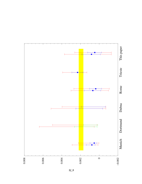
Figure 1: Compilation of recent theoretical predictions for $\varepsilon^{\prime}/\varepsilon$.

Lattice QCD [10]

In principle, Lattice QCD is the non-perturbative method for computing matrix elements. Being a regularized version of the fundamental theory, it allows a complete control over the definition of the renormalized operators, both at the perturbative and non-perturbative level. In addition, present simulations use inverse lattice spacings of $2$ GeV or larger and therefore the perturbative matching with the Wilson coefficients can be safely performed. Indeed, by using non-perturbative renormalization techniques, the matching scale in lattice calculations could be pushed to values as large as $\sim 10$ GeV. Although, so far, these methods have only been implemented in the calculation of the strong coupling constant [11] and of the quark masses [12], they will certainly be extended to the four-fermion operators of the weak effective Hamiltonian. When this will be the case, the error in the matching procedure will become negligible.

For many years, a general no-go theorem [13] of Euclidean field theory has prevented the direct extraction, in numerical simulations, of the physical matrix elements with more than one particle in the final state. For this reason, present lattice determinations of $\langle\pi\pi|Q_{i}|K\rangle$ are obtained from $\langle\pi|Q_{i}|K\rangle$ using lowest-order chiral relations (i.e. soft-pion theorems). This means that final-state interactions are not taken into account and that large chiral corrections may be present [14] . In addition, only some of the matrix elements needed for computing $\varepsilon^{\prime}/\varepsilon$ are presently available. In particular, the $Q_{6}$ matrix element, which is expected to give the most important contribution to $\varepsilon^{\prime}/\varepsilon$, has not been successfully computed yet.

Several theoretical progresses have opened a window of opportunity this year. In the past, a proposal to circumvent the no-go theorem of ref. [13] was made. The main idea was to extract the relevant matrix elements by studying suitable Euclidean Green functions at small time distances [15]. The weakness of this method, however, was that it relied on model-dependent smoothness assumptions which could lead to uncontrolled systematic errors. A big progress has been made in ref. [16], where it was rigorously proven how to relate the matrix elements extracted on a finite volume in lattice simulations to the physical $\langle\pi\pi|Q_{i}|K\rangle$ amplitudes. Moreover, it has been shown that the smoothness hypothesis of ref. [15] is unnecessary and that the physical $K\to\pi\pi$ matrix elements can be, at least in principle, extracted from Euclidean correlation functions at finite-time distances [17]. Although it will take some time before these approaches will be implemented in practice, they certainly open new perspectives to lattice calculations.

More details on the present status of lattice matrix elements, and possible developments in the near future, will be given in the discussion of the phenomenological analysis in the next section.

Phenomenological Approach [18]

In this approach, one basically attempts to extract information on the matrix elements relevant for $\varepsilon^{\prime}/\varepsilon$ by combining the measured values of the $CP$-conserving amplitudes with relations among different operators that can be established below the charm threshold under very mild assumptions (for details see ref. [19]). This procedure can be performed consistently at the NLO, allowing the extraction of matrix elements of well-defined renormalized operators.

Unfortunately, the leading contributions to $\varepsilon^{\prime}/\varepsilon$, namely the matrix elements of $Q_{6}$ and $Q_{8}^{3/2}$, cannot be fixed in this approach. Moreover, the method only works below the charm threshold where higher-order perturbative and power corrections (in $1/m_{c}$) may be large. In practice, for these matrix elements, Buras and collaborators have always used inputs coming from other theoretical sources, in particular lowest-order $1/N$ expansion or lattice calculations.

Chiral+$1/N$ Expansion [20]

This method relies on the non-perturbative technique originally proposed by Bardeen, Buras and Gérard [21]. In principle, the approach can be derived from QCD and allows the computation of all the matrix elements needed for calculating $\varepsilon^{\prime}/\varepsilon$ in a consistent theoretical scheme. In this framework, the Dortmund group computed the relevant matrix elements including the subleading corrections in both the chiral and the $1/N$ expansion .

This approach suffers, however, from the presence of quadratic divergences in the cutoff that must be introduced, beyond the leading order, in the effective chiral Lagrangian. The quadratic cutoff dependence, which appears in non-factorizable contributions, makes it impossible a consistent matching between the operator matrix elements and the corresponding Wilson coefficients, which depend only logarithmically on the cutoff. One may argue that the quadratic divergences will be cured and replaced by some hadronic scale in the full theory, which includes excitations heavier than the pseudoscalar mesons. In practice, since it is impossible to include the effects of higher-mass hadronic states, the cutoff is replaced with a scale of the order of 1 GeV, which is an arbitrary, although reasonable, choice. Since the divergent terms gives very large contributions to the matrix elements entering $\Delta I=1/2$ transitions and $\varepsilon^{\prime}/\varepsilon$, this introduces an uncontrolled numerical uncertainty in the final results.

Chiral Quark Model [22]

The $\chi$QM can be derived in the framework of the extended Nambu-Jona-Lasinio model of chiral symmetry breaking [22]. It contains an effective interaction between the $u$, $d$, $s$ quarks and the pseudo-scalar meson octet with three free parameters, two of which can be fixed using $CP$-conserving amplitudes. The Trieste group computed the ${\cal O}(p^{4})$ corrections to the relevant operators and found a correlation between the $CP$-conserving and $CP$-violating amplitudes so that, once the parameters of the model are fixed to provide the required octet enhancement, it is possible to predict $\varepsilon^{\prime}/\varepsilon$. The nice feature of this model is that, to some extent, it accounts for higher-order chiral effects, which are not easily included, for instance, in lattice calculations. The disadvantage is that the model dependence of the results can hardly be evaluated or corrected.

Theoretically, this approach shares some of the problems of the $1/N$ expansion mainly those related to the presence of quadratic divergences. These do not appear explicitly in the calculations of the Trieste group simply because dimensional regularization is used. It remains true, however, that the scale and scheme dependence of the renormalized operators is not under control at NLO. In order to deal with this problem, a third parameter of the model is fixed by imposing a sort of numerical “$\gamma_{5}$”-independence to the physical amplitudes. This recipe, while suggesting that some degree of “effective” renormalization-scheme independence can be achieved, has unfortunately no sound theoretical basis. Finally the correlation between the $\Delta I=1/2$ amplitude and $\varepsilon^{\prime}/\varepsilon$ is subject to potentially large uncertainties for the following reason. The parameters necessary to estimate the matrix element of $Q_{6}$ are fixed by fitting the $\Delta I=1/2$ amplitude. For this quantity, the contribution of $Q_{6}$ is rather marginal, whereas $Q_{1}$ and $Q_{2}$ dominate. Thus any small uncertainty in the dominant terms, due for example to unknown ${\cal O}(p^{6})$ corrections (${\cal O}(p^{4})$ corrections to the $\Delta I=1/2$ amplitude are of ${\cal O}(100\%)$), may change drastically the determination of the matrix element of $Q_{6}$, which is the dominant term for $\varepsilon^{\prime}/\varepsilon$.

Extended Nambu-Jona-Lasinio Model [23]

An extended Nambu-Jona-Lasino model has been used in ref. [23] to compute the $\Delta I=1/2$ $K\to\pi\pi$ matrix elements and $\varepsilon^{\prime}/\varepsilon$. The remarkable feature of this computation is the high order in the momentum expansion reached by the Dubna group. All matrix elements have been computed to ${\cal O}(p^{6})$ and a good stability of the results has been found. In this respect, this approach is safer than the $\chi$QM. However it shares with the $\chi$QM all the other theoretical flaws mentioned above, and particularly the problem of matching the short-distance calculations, since it is unclear which renormalized operators the amplitudes computed with the Dubna superpropagator regularization method correspond to.

Generalized Factorization [24]

Generalized factorization has been introduced in the framework of non-leptonic $B$ decays in order to parametrize the hadronic matrix elements without a-priori assumptions [25]. The basic idea is to extract from experimental data as much information as possible on the non-factorizable parameters. When needed, the number of independent parameters can be reduced using flavour symmetries, dynamical assumptions, etc. In ref. [24] the procedure has been applied to $K\to\pi\pi$ matrix elements. Unfortunately, in this case, the number of independent channels that one can use to fix the parameters is small (essentially only the two $CP$-conserving amplitudes). For his predictions, the author of ref. [24] was forced then to reduce the number of parameters by several “simplifying” assumptions, which are, however, questionable. Many parameters related to different operator matrix elements and to different colour structures were arbitrarily assumed to be equal. In such a way, a correlation between $CP$-conserving and $CP$-violating amplitudes was obtained, but the final results crucially depends on the assumptions, which are hardly justifiable theoretically, and cannot be tested phenomenologically in processes different from $\varepsilon^{\prime}/\varepsilon$.

$\sigma$ Models [7, 26]

A possible mechanism to enhance the $\Delta I=1/2$ amplitude is the exchange of a scalar $I=0$ meson [27]. It also leads to an enhancement of $\varepsilon^{\prime}/\varepsilon$, as recently studied in the framework of the linear [7] and non-linear [26] $\sigma$ models. While unable to achieve NLO accuracy, these models can produce the required correlation between the $\Delta I=1/2$ rule and $\varepsilon^{\prime}/\varepsilon$, at least for some choice of the free parameters, such as the $\sigma$ mass. Also in this case, however, it is not easy to estimate the uncertainties and the model dependence of the theoretical predictions.

Other theoretical developments

The marginal agreement between the SM predictions and the measured value of $\varepsilon^{\prime}/\varepsilon$ stimulated various attempts to “improve” the determination of the operator matrix elements, by including effects that were not considered previously. In particular, new studies have been devoted to the calculation of isospin-breaking and final-state interaction effects.

In most of the approaches isospin-breaking corrections are not included because they are beyond reach for these methods. These effects can be evaluated, however, a posteriori and included in the predictions. The leading effect in the chiral expansion is expected to come from $\pi$–$\eta$–$\eta^{\prime}$ mixing, which can be computed following ref. [5]. The resulting isospin-breaking effect is accounted for by the parameter $\Omega_{IB}$ which appears in eq. (9). Recently the calculation of $\Omega_{IB}$ has been updated by including the effect of $\pi^{0}-\eta$ mixing at ${\cal O}(p^{4})$ [28]. In addition, it has been pointed out in ref. [29] that new sources of isospin breaking appear, beyond the leading order, in the chiral Lagrangian. These terms may give large corrections to $\Omega_{IB}$. Unfortunately the calculation of the corrections is strongly model dependent and can only been taken as a warning on the potential importance of these effects.

The problem of including final-state interactions is particularly relevant for lattice or lowest-order $1/N$ calculations, where rescattering effects are missing. It has recently been suggested that these effects could be included by using the measured $\pi\pi$ phase shifts and dispersive techniques [14]. The resulting $A_{0}$ amplitude would be enhanced by the inclusion of final state interactions, giving for $\varepsilon^{\prime}/\varepsilon$ a prediction much closer to the experimental value. These approach have been subject to several criticisms [30]. On the one hand the analytic structure of the considered amplitudes is unclear and the corresponding dispersion relations questionable. On the other, the computation of the dispersive correction factors, as derived in ref. [14], is plagued by an irreducible ambiguity of the same order of the dispersive factors themselves. This uncertainty depends on the choice of the initial conditions which, as shown in [30], were arbitrarily chosen. For this reason, whereas final-state interactions are likely to give qualitatively a certain enhancement, as argued in ref. [14], the quantitative estimate of these effect is subject to very large uncertainties. As discussed in [30], lattice calculations could help in this respect by fixing the initial conditions in a unambiguous way.

Some short, provocative comment is necessary at this point. If one could implement in the same calculation all the corrections which have been suggested to improve the accuracy in the determination of the matrix elements (low strange-quark mass, isospin-breaking effects, final state interactions, etc.), one would probably end up with a prediction of $\varepsilon^{\prime}/\varepsilon$ much larger than its experimental value. It is also quite astonishing that the effects which were not considered before, or those which have been revised in recent studies, all increase the theoretical prediction for this quantity and no one goes in the opposite direction. Finally, if the $\Delta I=1/2$ rule and the large value of $\varepsilon^{\prime}/\varepsilon$ are a consequence of many effects which are all necessary in a conspiracy to give a large enhancement, it seems very unlikely that any of the existing theoretical approaches (including the lattice one), will ever be able to take them into account simultaneously at the necessary level of accuracy.

During the completion of this paper, several new calculations of $\varepsilon^{\prime}/\varepsilon$ appeared: i) a new estimate of the $Q_{6}$ and $Q_{8}^{3/2}$ matrix elements using QCD sum rules has been presented [31], with results for $\varepsilon^{\prime}/\varepsilon$ close to the experimental average; ii) within big uncertainties, very large values of $\varepsilon^{\prime}/\varepsilon$ have also been obtained using the $1/N$ and chiral expansions within the context of the extended Nambu-Jona-Lasinio model. In ref. [32], the proposal for controlling the scale and scheme dependence of renormalized operators using an intermediate $X$-boson has been implemented in the calculation of $\varepsilon^{\prime}/\varepsilon$. We refer the reader to the original publications for more details.

5 Results for $\varepsilon^{\prime}/\varepsilon$ using Lattice QCD

In order to compute $\varepsilon^{\prime}/\varepsilon$, besides hadronic matrix elements one needs the value of the relevant combination of CKM matrix elements, namely Im$V_{ts}^{\star}V_{td}$. This is constrained by using the experimental information on $|V_{cb}|$, $|V_{ub}|$, $B_{d,s}$–$\bar{B}_{d,s}$ mixings and $\varepsilon$ combined with lattice results. Nowadays this has become a standard way of determining the CKM-matrix parameters within the Standard Model, described for instance in refs. [10, 33]. It is worth noting that the linear dependence of $\varepsilon^{\prime}/\varepsilon$ on Im$V_{ts}^{\star}V_{td}$ is strongly reduced by the constraint on the CKM parameters enforced by the measured value of $\varepsilon$. In the analysis reported in this paper, the same input parameters as in ref. [10], with the exception of $\Omega_{IB}=0.16\pm 0.03$ which is now taken from [28], have been used.

The discussion in ref. [10] about the current status of the lattice computation of the main matrix elements $\langle\pi\pi|Q_{6}|K\rangle$ and $\langle\pi\pi|Q_{8}^{3/2}|K\rangle$ can be summarized as follows:

• At present, the matrix element $\langle\pi\pi|Q_{6}|K\rangle$ is not reliably known from lattice QCD. The results with staggered fermions are plagued by huge corrections appearing in the operator renormalized using lattice perturbation theory [34]. Other attempts using Wilson fermions or domain-wall fermions were unsuccessful so far.

• The matrix element $\langle\pi\pi|Q_{8}^{3/2}|K\rangle$ has been computed by several groups using different formulations of the lattice fermion action and different lattice spacing. A substantial agreement of the different determinations was found within $20\%$ uncertainty. We use the value

  $$\langle\pi\pi|Q_{8}^{3/2}(2\,\mbox{GeV},\overline{\mbox{MS}}\mbox{-HV})|K\rangle=0.62\pm 0.12\,\mbox{GeV}^{3}$$ (15)

  for the operator renormalized at $\mu=2$ GeV in the ’t Hooft-Veltman $\overline{\mbox{MS}}$ scheme. This value corresponds to the $B$ parameter $B_{8}^{3/2}=0.93\pm 0.18$ for a “conventional” quark mass $m_{s}^{\overline{\mbox{\scriptsize MS}}}+m_{d}^{\overline{\mbox{\scriptsize MS}}}=130$ MeV at $\mu=2$ GeV, see eq. (13).

Using some reasonable assumptions for the less important contributions due to other operators, given that the largest uncertainty stems from our ignorance of $\langle\pi\pi|Q_{6}|K\rangle$, a useful way of presenting the results is given by

$$\frac{\varepsilon^{\prime}}{\varepsilon}=\left[(-25.3^{+3.1}_{-3.6})\,\mbox{GeV}^{-3}\,\langle\pi\pi|Q_{6}(2\,\mbox{GeV},\overline{\mbox{MS}}\mbox{-HV})|K\rangle-6.3^{+1.6}_{-1.7}\right]\times 10^{-4}\,,$$ (16)

where the matrix element of $Q_{6}$ is considered as a free parameter. Notice that the the two terms in this equation are correlated and should not be varied independently.

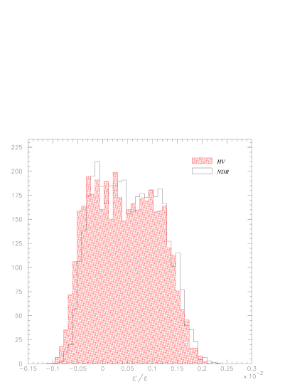
Figure 2: Distribution of values for $\varepsilon^{\prime}/\varepsilon$ using $B_{6}=1\pm 1$ either in $\overline{\mbox{MS}}\mbox{-HV}$ or in $\overline{\mbox{MS}}\mbox{-NDR}$ as discussed in the text.

In order to compare eq. (16) with experiments, we have to make some assumption on the value of $\langle\pi\pi|Q_{6}|K\rangle$. We take the central value suggested by the $VIA$ (or equivalently by the lowest-order $1/N$ expansion), namely $B_{6}=1$, with an uncertainty of $100\%$. This introduce a renormalization-scheme ambiguity, since $VIA$ does not allow a proper definition of the renormalized operators. For this reason, results obtained by taking two different central values for $\langle\pi\pi|Q_{6}|K\rangle$ (corresponding either to $B_{6}^{\mbox{\scriptsize HV}}(2$ GeV)=1 or to $B_{6}^{\mbox{\scriptsize NDR}}(2$ GeV)=1 are presented, namely

$$\langle\pi\pi|Q_{6}(2\,\mbox{GeV},\overline{\mbox{MS}}\mbox{-HV})|K\rangle=-0.4\pm 0.4\,\mbox{GeV}^{3}$$ (),

().

(17)

In the two cases, we obtain

$$\varepsilon^{\prime}/\varepsilon=(4.6^{+7.7}_{-7.2}\pm 0.4)\times 10^{-4}$$ Monte Carlo

scanning

Monte Carlo

scanning

(18)

The difference of the two results, contrary to what is often stated in the literature, is not the uncertainty associated to the renormalization-scheme dependence, but to a different choice of the value of the matrix element in a given scheme (the HV scheme in the example of eq. (17)). At the NLO, the scheme dependence comes from higher-order corrections only and its effect is estimated by the second error given in eq. (LABEL:eq:res). The two figures of eq. (LABEL:eq:res) correspond really to two different choices of the unknown value of $\langle\pi\pi|Q_{6}|K\rangle$ at a given scale ($\mu=2$ GeV) and in a well-defined scheme ($\overline{\mbox{MS}}\mbox{-HV}$). On the contrary, the two distributions of values for $\varepsilon^{\prime}/\varepsilon$ in fig. 2 include, for the same choice of $\langle\pi\pi|Q_{6}|K\rangle$, two different ways to match Wilson coefficients and matrix elements for estimating the real scheme dependence due to higher-order terms. Both distributions refer to the case $B_{6}(2\,\mbox{GeV},\overline{\mbox{MS}}\mbox{-HV})=1\pm 1$. The large error on the matrix elements of $Q_{6}$ obviously dominates the final uncertainty on $\varepsilon^{\prime}/\varepsilon$ and flattens these distributions. In ref. [18] a more optimistic error for the $B$ parameter ($B_{6}(2\,\mbox{GeV},\overline{\mbox{MS}}\mbox{-HV})=1\pm 0.2$) was assumed.

6 Comparison with data

Many of the Standard Model predictions shown in fig. 1 are below the present experimental world average. What does this imply? There are three legitimate answers:

1. There is nothing wrong! For some specific choice of the input parameters, all the different approaches are able to reproduce to some extent the experimental data. In some cases the agreement seems to arise naturally from the calculation [31, 32]. In other cases, this requires the adjustment of a few parameters [22] or a wise choice of several of them (often at the edge of the allowed range of values) [18, 10]. It is puzzling that most of the approaches, which suffer from intrinsic and irreducible uncertainties coming from the model dependence of the results, are in good agreement with the data. In the case of refs. [10, 18], instead, this requires that all the quantities on which we have a poor control conspire in the direction to increase the theoretical value of $\varepsilon^{\prime}/\varepsilon$. Thus, although unlikely in our opinion, the possibility that there is nothing wrong is not excluded. It may also well be that some of the models are indeed able to describe the underlying strong dynamics.

2. There is something missing in the computation of the matrix elements. The long-standing problem of explaining the $\Delta I=1/2$ rule suggests that some important dynamical effect is at work in $K\to\pi\pi$ $I=0$ decays. Unfortunately, contrary to some old claim, there is no simple relation between the $CP$-conserving and $CP$-violating decays, which could explain the large value of $\varepsilon^{\prime}/\varepsilon$ on the basis of the enhancement of the $\Delta I=1/2$ amplitude. Indeed, it would be very interesting if a common dynamical mechanism could explain both of them. In terms of Wick contractions in the matrix elements, such a mechanism could be possibly provided by a large contribution from eye diagrams (aka penguin contractions) [35]. From the lattice estimates, by taking $B_{6}$ as a free parameter, we can reproduce the experimental $\varepsilon^{\prime}/\varepsilon$ with $B_{6}^{\mbox{\scriptsize HV}}(2\,\mbox{GeV})\sim 2.4$. As we have seen, all non-perturbative methods are affected by theoretical and/or computational problems which limit their accuracy. Among them, the models based on the chiral expansion also support the existence of some correlation between the $\Delta I=1/2$ rule and $\varepsilon^{\prime}/\varepsilon$ which is at least in qualitative agreement with the observations. A possible exception is that of ref. [23]. Thus we conclude that a real quantitative explanation is still to come.

3. Hadronic matrix elements are fine. New physics is at work. If the theoretical calculations which gives low values for $\varepsilon^{\prime}/\varepsilon$ are correct, there is room for new physics effects. It is not difficult to imagine new sources of $CP$ violation. In supersymmetry, for example, there are even too many. The problem is that we must find a model for new physics such as to obtain a sizeable contribution to $\varepsilon^{\prime}/\varepsilon$ while remaining within the stringent constraints imposed by $\varepsilon$ and by other measured quantities. This problem can be circumvented, so that for instance supersymmetry is potentially able (with some special assumptions) to produce the required effect on $\varepsilon^{\prime}/\varepsilon$ still fulfilling the other phenomenological constraints [36].

At present, our preferred answer is the second one. Hopefully, improvements in non-perturbative techniques and a further insight in kaon phenomenology will clarify the mechanism responsible for the “large” value of $\varepsilon^{\prime}/\varepsilon$ and its connections with the $\Delta I=1/2$ rule.

References

- [1] A. Alavi-Harati et al., Phys. Rev. Lett. 83 (1999) 22.
- [2] A. Ceccucci, CERN Particle Physics Seminar (29 February 2000), http://www.cern.ch/NA48/Welcome/images/talks/cern00/talk.ps.gz.
- [3] G. D’Agostini, CERN-EP-99-139, hep-ex/9910036.
- [4] E. Chell and M.G. Olsson, Phys. Rev. D48 (1993) 4076.
- [5] A.J. Buras and J.-M. Gérard, Phys. Lett. B192 (1987) 156.
- [6] A.J. Buras, M. Jamin and M.E. Lautenbacher and P.H. Weisz, Nucl. Phys. B400 (1993) 37; A.J. Buras, M. Jamin and M.E. Lautenbacher, ibid. 75; M. Ciuchini, E. Franco, G. Martinelli and L. Reina, Nucl. Phys. B415 (1994) 403.
- [7] Y.-Y. Keum, U. Nierste and A.I. Sanda, Phys. Lett. B457 (1999) 157.
- [8] A. Donini et al., Phys. Lett. B470 (1999) 233.
- [9] M. Ciuchini et al., hep-ph/9910237, to appear in: Proc. of KAON ‘99, June 21–26 1999, Chicago, USA.
- [10] M. Ciuchini et al., Nucl. Phys B573 (2000) 201.
- [11] M. Lüscher, Les Houches Lectures on “Advanced Lattice QCD”, hep-lat/9802029, and refs. therein.
- [12] J. Garden et al., Nucl. Phys. B571 (2000) 237.
- [13] B.Yu. Blok and M.A. Shifman, Sov. J. Nucl. Phys. 45 (1987) 522; L. Maiani and M. Testa, Phys. Lett. B245 (1990) 585.
- [14] E. Pallante and A. Pich, Phys. Rev. Lett. 84 (2000) 2568; E. Paschos, hep-ph/9912230.
- [15] M. Ciuchini, E. Franco, G. Martinelli and L. Silvestrini, Phys. Lett. B380 (1996) 353
- [16] L. Lellouch and M. Lüscher, hep-lat/0003023.
- [17] Talk by C.T. Sachrajda at the Ringberg Workshop on Non-perturbative Methods, Ringberg, April 2-8, 2000; G. Martinelli and C.T. Sachrajda, to appear.
- [18] S. Bosch et al., Nucl. Phys. B565 (2000) 3.
- [19] A.J. Buras, M. Jamin and M.E. Lautenbacher, Nucl. Phys. B408 (1993) 209.
- [20] T. Hambye, G.O. Köhler, E.A. Paschos and P.H. Soldan, Nucl. Phys. B564 (2000) 391.
- [21] W.A. Bardeen, A.J. Buras and J.-M. Gérard, Phys. Lett. B180 (1986) 133; W.A. Bardeen, A.J. Buras and J.-M. Gérard, Phys. Lett. B192 (1987) 138; W.A. Bardeen, A.J. Buras and J.-M. Gérard, Phys. Lett. B211 (1988) 343.
- [22] S. Bertolini, J.O. Eeg and M. Fabbrichesi, hep-ph/0002234 and refs. therein..
- [23] A.A. Bel’kov, G. Bohm, A.V. Lanyov and A.A. Moshkin, hep-ph/9907335.
- [24] H.-Y. Cheng, hep-ph/9911202.
- [25] M. Neubert and B. Stech, CERN-TH-97-099, in Heavy flavours II, A. Buras and M. Lindner eds., p. 294, hep-ph/9705292.
- [26] M. Harada et al., hep-ph/9910201.
- [27] M.B. Gavela et al., Phys. Lett. B211 (1988) 139.
- [28] G. Ecker, G. Müller, H. Neufeld and A. Pich, Phys. Lett. B477 (2000) 88.
- [29] S. Gardner and G. Valencia, Phys. Lett. B466 (1999) 355.
- [30] A.J. Buras et al., Phys. Lett. B480 (2000) 80.
- [31] S. Narison, hep-ph/0004247.
- [32] J. Bijnens and J. Prades, JHEP 0001 (2000) 002; J. Bijnens and J. Prades, hep-ph/0005189.
- [33] P. Paganini, F. Parodi, P. Roudeau and A. Stocchi, Phys. Scripta V. 58 (1998) 556; F. Parodi, P. Roudeau and A. Stocchi, Nuovo Cim. 112A (1999) 833; F. Caravaglios, F. Parodi, P. Roudeau and A. Stocchi, hep-ph/0002171; S. Mele, Phys. Rev. D59 (1999) 113011; A. Ali and D. London, Eur. Phys J. C9 (1999) 687; M. Bargiotti et al., La Rivista del Nuovo Cimento, Vol. 23, N.3 (2000), 1; S. Plaszczynski, M.-H. Schune, hep-ph/9911280.
- [34] S. Sharpe et al., Phys. Lett. 192B (1987) 149; S. Sharpe and A. Patel, Nucl. Phys. B417 (1994) 307; N.Ishizuka and Y. Shizawa, Phys. Rev. D49 (1994) 3519; D. Pekurovsky and G. Kilcup, Nucl. Phys. Proc. Suppl. 63 (1998) 293; D. Pekurovsky and G. Kilcup, hep-lat/9812019.
- [35] M. Ciuchini, E. Franco, G. Martinelli and L. Silvestrini, hep-ph/9909530, to appear in: Proc. of KAON ‘99, June 21–26 1999, Chicago, USA.
- [36] A. Masiero and O. Vives, hep-ph/0001298 and refs. therein.