A Topcolor Jungle Gym

Abstract

We discuss an alternative to the topcolor seesaw mechanism. In our scheme, all the light quarks carry topcolor, and there are many composite $SU(2)$ doublets. This makes it possible to get the observed $t$ quark mass and observed $SU(2)\times U(1)$ breaking in a way that is quite different from the classic seesaw mechanism. We discuss a model of this kind that arises naturally in the context of dynamically broken topcolor. There are many composite scalars in a theory of this kind. This has important effects on the Pagels-Stokar relation and the Higgs mass. We find $m_{\rm Higgs}\raisebox{1.99997pt}{$\hbox to0.0pt{\raisebox{-5.0pt}{$\;\sim$}\hss}<\,$}330$ GeV, lighter than in typical topcolor models. We also show that the electroweak singlet quarks in such a model can be lighter than the corresponding quarks in a seesaw model.

1 Topcolor

We have known for many years that the weak interactions are associated with the exchange of a massive gauge boson associated with a spontaneously broken $SU(2)\times U(1)$ symmetry. The Goldstone bosons of the symmetry breaking are eaten by the Higgs mechanism to become the longitudinal components of the massive gauge bosons. But the nature of the Goldstone bosons remains mysterious. Although there are fascinating hints that the Goldstone bosons might be fundamental bosons from grand unified supermultiplets [1], it is still possible that some more complicated dynamics is involved. The simplest versions of strong dynamics are ruled out [2], so we know that if a strong coupling scheme is to work, it must be very different from QCD.

Topcolor [3] is a speculative scheme that may produce composite Goldstone bosons and a composite Higgs boson [4]. The idea is that if a strong topcolor gauge symmetry is spontaneously broken, there is a balance between the strong attractive gauge interaction that without spontaneous breaking would confine topcolored particles, and the effect of spontaneous breaking that liberates the topcolored particles by decreasing the range of the interaction in the Higgs phase. The hope is that the transition from the confining phase to the Higgs phase is smooth. If so, then we should be able to tune the strength of the symmetry breaking to produce a light composite scalar multiplet built out of the topcolored fermions. This composite multiplet can then contain the Goldstone bosons and a Higgs boson. There is no completely convincing proof of the required smoothness, but it is consistent with everything we know.

In section 2, we introduce our new topcolor model (which we call a “topcolor jungle gym”) and compare it with a classic seesaw model. The most obvious difference is that we have far more composite scalars below the topcolor scale. In the remaining sections, we discuss a variety of phenomenological issues that arise because of the large number composite scalars in our model. We discuss flavor-changing neutral current effects in section 3.1, the Pagels-Stokar relation in section 3.2, phenomenological constraints on the singlet quark masses in section 3.3, the size of the topcolor scale in section 4 and the Higgs mass and the stability of the vacuum in section 5. In appendix A, we work out a toy example of some of the physics that could give rise to quark masses.

2 Seesaw versus Jungle Gym

In the classic seesaw model [6], the left-handed $(t,b)$ doublet and a heavy right-handed particle, $\chi$, carry topcolor, and the Higgs multiplet is a bound state of these two. The mass of the $t$ results from mixing between the $t$ and the $\chi$, with the $t$ quark mass inversely related to the $\chi$ mass — hence the name. This scheme has some advantages [7], but is certainly not so compelling that we should ignore other possibilities.

In this note, we suggest a different scheme that emerged in our study of the possibility that topcolor itself may be broken dynamically [8]. With three or more heavy particles like the $\chi$ of the conventional seesaw model we have the option of having all the observed quarks carrying topcolor, as shown in moose notation [9] in figure 1.

....................................................................................................................................................................................................................................................................................................................................................................................................................................................................................................................................................................................................................................................................................................................................$$3_{TC} 3_{C} n_{\chi} n_{\omega} \xi_{R} \xi_{L} \psi^{j}_{L} \chi^{x}_{R} \omega^{a}_{R} \chi^{x}_{L} \omega^{a}_{L} U^{j}_{R} D^{j}_{R}$$+................................................................................................................................................................................................................................................................................................................................................................................................................................................................................................................................................................................................................................................................................................................................................................................................................................................................................................................................................................................................................................................................................................................................................................................

Figure 1: A Jungle-Gym Moose.

In a conventional notation, the moose of figure 1 describes the quarks of the standard model, the electroweak doublets $\psi^{j}_{L}$, and the singlets $U^{j}_{R}$ and $D^{j}_{R}$ for $j=1$ to 3, along with $n_{\chi}$ additional charge $2/3$ quarks, $\chi^{x}$ for $x=1$ to $n_{\chi}$, and $n_{\omega}$ additional charge $-1/3$ quarks, $\omega^{a}$ for $a=1$ to $n_{\omega}$. The gauge group is

$$SU(3)_{C}\times SU(3)_{TC}\times SU(n_{\chi}\mathord{+}n_{\omega})\times SU(2)\times U(1)$$ (2.1)

The transformation properties of the fermion fields (the directed lines in the moose diagram) are

$$\begin{array}[]{r@{\,:\;}l}\psi^{j}_{L}&(1,3,1,2)_{1/6}\\ U^{j}_{R}&(1,3,1,1)_{2/3}\\ D^{j}_{R}&(1,3,1,1)_{-1/3}\\ \chi^{x}_{R}&(1,3,1,1)_{2/3}\\ \omega^{a}_{R}&(1,3,1,1)_{-1/3}\\ \end{array}\quad\quad\begin{array}[]{r@{\,:\;}l}\xi_{L}&(3,1,n_{\chi}\mathord{+}n_{\omega},1)_{y}\\ \xi_{R}&(1,3,n_{\chi}\mathord{+}n_{\omega},1)_{y}\\ \chi^{x}_{L}&(3,1,1,1)_{2/3}\\ \omega^{a}_{L}&(3,1,1,1)_{-1/3}\\ \end{array}$$ (2.2)

where to cancel anomalies we need

$$y=-{2n_{\chi}-n_{\omega}\over 3(n_{\chi}\mathord{+}n_{\omega})}.$$ (2.3)

This is a “universal coloron” model [10] in the sense that all of the light quarks carry the topcolor interactions. The $\chi$ and $\omega$ quarks are required for anomaly cancellation, and as we will see, play a role in making the $t$ quark light. It is important that $n_{\chi}$+$n_{\omega}$ be greater than or equal to three, and that $n_{\chi}$ and $n_{\omega}$ be greater than zero, but otherwise, these are not tightly constrained.

In this model, the $\chi$ and $\omega$ play no direct role in the generation of mass for the observed quarks. Instead, among the many composite Higgs doublets are the following:

$$H_{U}^{m\overline{m}}\sim\overline{U}_{R}^{\overline{m}}\psi_{L}^{m},\quad\quad H_{D}^{m\overline{m}}\sim\overline{D}_{R}^{\overline{m}}\psi_{L}^{m}.$$ (2.4)

These have strong couplings to the quarks of which they are made with Yukawa couplings of the form

$$h\left(\overline{\psi}^{m}_{L}\,H_{U}^{m\overline{m}}\,U^{\overline{m}}_{R}+\overline{\psi}^{m}_{L}\,H_{D}^{m\overline{m}}\,D^{\overline{m}}_{R}\right)+\mbox{h.c.}$$ (2.5)

for large $h$ (in naive dimensional analysis, $h$ is of order $4\pi/\sqrt{3}$).

If the appropriate linear combination of these Higgs fields gets light and develops a vacuum expectation value (VEV), the strong Yukawa couplings produce the masses directly. The $\chi$ and $\omega$ may be important because Higgs doublets built out of them can provide additional breaking of the electroweak symmetry, to allow the Pagels-Stokar [11] formula to work for the $t$ quark (assuming, as we usually do for no very good reason, that the naive Pagels-Stokar formula is accurate — see section 3.2).

The mass matrix for the conventional seesaw model must get contributions from at least three different kinds of operators and couplings. However in the model of figure 1, there are only two kinds of terms because there is no difference except convention between $\chi_{R}$ and $U_{R}$. They transform in the same way under the topcolor and electroweak gauge symmetries, as you can see from (2.2). The mass matrix looks generically like

$$\pmatrix{\overline{\chi_{R}}&\overline{U_{R}}\cr}\,\pmatrix{x&y^{\prime}\cr x^{\prime}&y\cr}\,\pmatrix{\chi_{L}\cr U_{L}\cr},$$ (2.6)

where the repeated letters are intended to indicate that the mechanisms are the same for the $x$ and $x^{\prime}$ and (separately) for the $y$ and $y^{\prime}$. By purely conventional redefinitions of what is $\chi_{R}$ and and what is $U_{R}$ we can put zeros in (2.6) and write it either as

$$\pmatrix{\overline{\chi_{R}}&\overline{U_{R}}\cr}\,\pmatrix{x&y^{\prime}\cr 0&y\cr}\,\pmatrix{\chi_{L}\cr U_{L}\cr},$$ (2.7)

or as

$$\pmatrix{\overline{\chi_{R}}&\overline{U_{R}}\cr}\,\pmatrix{x&0\cr x^{\prime}&y\cr}\,\pmatrix{\chi_{L}\cr U_{L}\cr}.$$ (2.8)

The form in (2.7) is often the most useful, because we are typically interested in $x\gg y$, so it pays to diagonalize $x$.

There are a number of important consequences of the form (2.7).

First, we notice that all of the quarks can get masses from the dimension 6 operators. Of course, this is both good news and bad news. It means that we have a potentially realistic model, but also that there is no trivial explanation of the hierarchy of quark masses. This must come from the details of the flavor physics.

Second, the decoupling limit of the theory is very straightforward. If $x\gg y$, the light quark mass matrix is determined simply by the lower right-hand corner:

$$\pmatrix{\overline{\chi_{R}}&\overline{U_{R}}\cr}\,\pmatrix{x&y^{\prime}\cr 0&\framebox{$y$}\cr}\,\pmatrix{\chi_{L}\cr U_{L}\cr}.$$ (2.9)

The $y^{\prime}$ matrix in the upper right hand corner plays no role in the fermion mass spectrum in this limit, however, it is important in the Pagels-Stokar relation because the composite doublets whose VEVs contribute to this term also contribute to electroweak symmetry breaking.

Of course, the decoupling limit is also possible for the mass matrix of the conventional seesaw model, but it requires some tuning of the various different types of contributions to maintain the relation between the different types of terms in the mass matrix.

Note that because the difference between the $U_{R}$ and $\chi_{R}$ fields, and between the $D_{R}$ and $\omega_{R}$ fields is purely conventional (depending on the details of the flavor physics), it can be useful psychologically to combine them into multiplets, ${\cal U}_{R}$ and ${\cal D}_{R}$, and display the Moose as in figure 2.

....................................................................................................................................................................................................................................................................................................................................................................................................................................................................................................................................................................................................................................................................................................................................$$3 3 n_{\chi} n_{\omega} \xi_{R} \xi_{L} \psi^{j}_{L} {\cal U}^{r}_{R} {\cal D}^{s}_{R} \chi^{x}_{L} \omega^{a}_{L}$$+................................................................................................................................................................................................................................................................................................................................................................................................................................................................................................................................................................................................................................................................................................................................................................................................................................................................................................................................................................

Figure 2: The Moose of figure 1 in a notation in which the $U_{R}^{j}$ and $\chi_{R}^{x}$ fields are combined into a ${\cal U}_{R}^{r}$ multiplet (where $r$ runs from 1 to $n_{\chi}$+3), and the $D_{R}^{j}$ and $\omega_{R}^{a}$ fields are combined into a ${\cal D}_{R}^{s}$ multiplet (where $s$ runs from 1 to $n_{\omega}$+3).

The flavor physics in the model of figure 1 (or equivalently, figure 2) can be rather simple. No mass terms are allowed. One needs five types of 4-fermion operators —

$$\displaystyle\overline{\chi^{x}_{L}}\,\xi_{R}\;\overline{\xi_{L}}\,{\cal U}^{r}_{R},$$ (2.10)

$$\displaystyle\overline{\omega^{x}_{L}}\,\xi_{R}\;\overline{\xi_{L}}\,{\cal D}^{s}_{R},$$ (2.11)

$$\displaystyle\overline{\psi^{j}_{L}}\,{\cal U}^{r}_{R}\;\overline{\psi^{j^{\prime}}_{L}}\,{\cal D}^{s}_{R},$$ (2.12)

$$\displaystyle\overline{\psi^{j}_{L}}\,{\cal U}^{r}_{R}\;\overline{{\cal U}^{r^{\prime}}_{R}}\,\psi^{j^{\prime}}_{L},$$ (2.13)

$$\displaystyle\overline{\psi^{j}_{L}}\,{\cal D}^{s}_{R}\;\overline{{\cal D}^{s^{\prime}}_{R}}\,\psi^{j^{\prime}}_{L}.$$ (2.14)

The terms in (2.13) and (2.14) can arise from flavor gauge interactions, but (2.10-2.12) must come from more complicated flavor physics. Of the latter, (2.10) and (2.11) have a very simple structure and can be simply parameterized. On the other hand, the Peccei–Quinn-symmetry breaking terms in (2.12) involve a very large number of parameters. It may be possible to assume that all these terms are small. In appendix A, we work out a specific example in which the terms in (2.13) and (2.14) come from an $SO(3)$ gauge interaction. While we are unable to obtain a realistic mass matrix in this simple scheme, we do find a rich structure that we find encouraging.

3 Phenomenology

3.1 Flavor Violation

Below the topcolor scale, the $SU(3)\times SU(2)\times U(1)$ structure of this model is similar to that of a standard seesaw model. The differences here are that there are additional singlet quarks and more composite scalars. One might worry that the additional strongly coupled composite scalars will produce a host of unwanted flavor violating effects. However, this need not be the case. These effects will depend on the details of the flavor physics. The reason is that in the absence of flavor physics, the model has a large non-Abelian flavor symmetry acting on the topcolored quarks,

$$SU(3)_{L}\times SU(3\mathord{+}n_{\chi})_{U}\times SU(3\mathord{+}n_{\omega})_{D},$$ (3.15)

with the factors acting on the $\psi_{L}$, the ${\cal U}_{R}=U_{R}\mathord{+}\chi_{R}$ and the ${\cal D}_{R}=D_{R}\mathord{+}\omega_{R}$ multiplets, respectively. In fact, the symmetry of the strong interactions is still larger,

$$SU(6)_{L}\times SU(6\mathord{+}n_{\chi}\mathord{+}n_{\omega})_{U+D},$$ (3.16)

but (3.16) is broken down to (3.15) by the $SU(2)\times U(1)$ electroweak gauge interactions. The composite scalar doublets carry the transformation properties of the quarks out of which they are made, thus

$$H_{\cal U}^{m\overline{m}}\sim\overline{{\cal U}}_{R}^{\overline{m}}\psi_{L}^{m}$$ (3.17)

transforms like an electroweak doublet (with hypercharge $Y=-1/2$) and like $(3,\overline{3\mathord{+}n_{\chi}})$ under (3.15) and

$$H_{\cal D}^{m\overline{m}}\sim\overline{{\cal D}}_{R}^{\overline{m}}\psi_{L}^{m}$$ (3.18)

transforms like an electroweak doublet (with $Y=1/2$) and like $(3,\overline{3\mathord{+}n_{\omega}})$ under (3.15). The combination,

$$H=\pmatrix{H_{\cal U}&H_{\cal D}\cr}$$ (3.19)

transforms like a $(6,\overline{6\mathord{+}n_{\chi}\mathord{+}n_{\omega}})$ under (3.16). In terms of (3.19), the Yukawa couplings to the quarks look like

$$h\,\overline{\psi}_{L}\,H\,\pmatrix{{\cal U}_{R}\cr{\cal D}_{R}\cr}+\mbox{h.c.}$$ (3.20)

In particular the $H_{\cal U}$ and $H_{\cal D}$ composite scalar doublets are degenerate to lowest order in the absence of flavor physics. Now suppose that the flavor physics picks out a single linear combination of these scalar doublets and makes it light - with a slightly negative mass squared, so that this linear combination contains the Higgs boson and the Goldstone bosons of the standard model. Now we will show that all the extra doublets really do not introduce any additional flavor violation beyond that associated in a well defined sense with the exchange of the single Higgs multiplet. This is an overly simplistic picture of what the flavor physics does, to be sure, but it will illustrate the point that the extra flavor symmetry will in general suppress flavor changing effects. The idea of the demonstration is simple. Because of the large flavor symmetry, composite scalar exchange does not produce flavor violation if the scalars are all degenerate. If one linear combination has a different mass, it is only that difference that produces flavor violation. We will show more formally how this works below.

In general, we can write the properly normalized linear combination of scalar doublets that gets light as

$$\phi_{1}=\cos\theta\,H_{u}+\sin\theta\,\tilde{H}_{d},$$ (3.21)

where

$$\tilde{\phi}\equiv i\tau_{2}\,\phi^{*},$$ (3.22)

and

$$H_{u}\equiv\mathop{\rm tr}\Bigl{(}u^{\dagger}\,H_{\cal U}\Bigr{)}\quad\mbox{and}\quad H_{d}\equiv\mathop{\rm tr}\Bigl{(}d^{\dagger}\,H_{\cal D}\Bigr{)},$$ (3.23)

for a $3$$\times$$(3\mathord{+}n_{\chi})$ matrix $u$ and a $3$$\times$$(3\mathord{+}n_{\omega})$ matrix $d$ satisfying

$$\mathop{\rm tr}\Bigl{(}u\,u^{\dagger}\Bigr{)}=\mathop{\rm tr}\Bigl{(}d\,d^{\dagger}\Bigr{)}=1.$$ (3.24)

It is useful to define also the following fields:

$$\phi_{2}=\sin\theta\,H_{u}-\cos\theta\,\tilde{H}_{d},$$ (3.25)

$$H_{\hat{{\cal U}}}\equiv H_{\cal U}-u\,H_{u},\quad\quad H_{\hat{{\cal D}}}\equiv H_{\cal D}-d\,H_{d}.$$ (3.26)

In terms of these fields, we can write

$$H_{\cal U}=H_{\hat{{\cal U}}}+u\,(\cos\theta\,\phi_{1}+\sin\theta\,\phi_{2}),$$ (3.27)

$$H_{\cal D}=H_{\hat{{\cal D}}}+d\,(\cos\theta\,\tilde{\phi}_{2}-\sin\theta\,\tilde{\phi}_{1}).$$ (3.28)

The important point about (3.27) and (3.28) is they show exactly how $\phi_{1}$ appears in the matrix structure of (3.20).

Now to see the result, it is convenient to add two more fields, both with exactly the same couplings as $\phi_{1}$, call them $\phi^{\prime}_{1}$ and $\phi^{\prime\prime}_{1}$. Both $\phi^{\prime}_{1}$ and $\phi^{\prime\prime}_{1}$ are degenerate with $\phi_{2}$ and all the other composite doublets except $\phi_{1}$. But we choose $\phi^{\prime\prime}_{1}$ to be a ghost field, so that its effect cancels that of $\phi^{\prime}_{1}$. The point is that we can now group $\phi^{\prime}_{1}$ with $\phi_{2}$, $H_{\hat{{\cal U}}}$ and $H_{\hat{{\cal D}}}$ into a complete degenerate multiplet under the (3.16) flavor symmetry. Thus the couplings of these scalars produce no flavor change. All the flavor change comes from the propagation of $\phi_{1}$ and $\phi^{\prime\prime}_{1}$, which have the same couplings. This is the sense in which, as promised, the flavor violation is related to that produced by $\phi_{1}$ alone.

3.2 The Pagels-Stokar relation

In this section we discuss the constraint on the quark mass matrix in this model coming from the analog of the Pagels-Stokar relation. In this context, the Pagels-Stokar relation is essentially a formula for the Yukawa couplings of the composite Higgs. In this model, because of the large flavor symmetry, (3.16), it becomes a relation for the sum of the squares of all the terms in the quark mass matrix involving the left handed quark doublets. We can see this very simply using the formalism developed in section 3.1.

The masses of the charge $2/3$ and charge $-1/3$ quarks have the following form:

$$\pmatrix{\overline{{\cal U}_{R}}\cr}\,\pmatrix{X_{u}&Y_{u}\cr}\,\pmatrix{\chi_{L}\cr U_{L}\cr},\quad\quad\pmatrix{\overline{{\cal D}_{R}}\cr}\,\pmatrix{X_{d}&Y_{d}\cr}\,\pmatrix{\omega_{L}\cr D_{L}\cr},$$ (3.29)

where $X_{u}$ (a $(3$+$n_{\chi})$$\times$$n_{\chi}$ matrix) and $X_{d}$ (a $(3$+$n_{\omega})$$\times$$n_{\omega}$ matrix) are the contributions to the singlet masses and $Y_{u}$ (a $(3$+$n_{\chi})$$\times$$3$ matrix) and $Y_{d}$ (a $(3$+$n_{\omega})$$\times$$3$ matrix) are contributions to the masses from $SU(2)\times U(1)$ breaking.

Let $\phi_{1}$ from (3.21) be the linear combination of composite Higgs doublets that develops a vacuum expectation value. It is then clear from (3.27), (3.28) and (3.20) that the symmetry breaking mass matrices have the form

$$Y_{u}=h\,u\,v\cos\theta/\sqrt{2},\quad\quad Y_{d}=h\,d\,v\sin\theta/\sqrt{2}.$$ (3.30)

Thus using (3.24) we immediately conclude

$$\mathop{\rm tr}\Bigl{(}Y_{u}\,Y_{u}^{\dagger}\Bigr{)}+\mathop{\rm tr}\Bigl{(}Y_{d}\,Y_{d}^{\dagger}\Bigr{)}=h^{2}\,v^{2}/2.$$ (3.31)

Thus the sum of the squares of the $SU(2)\times U(1)$ breaking mass terms are determined by the square of coupling $h$. This coupling should be evaluated at a scale of the order of $\Lambda\approx 1$ TeV, the electroweak breaking scale. If the coupling at the topcolor scale, $\Lambda_{TC}$, is $h(\Lambda_{TC})$, then the coupling runs via the renormalization group down to a smaller value at the scale $\Lambda$. In our theory, all of the composite scalars in the low energy theory and all the quarks to which they couple contribute to the running of $h$. The running is thus not the same as in the simple seesaw model, and it depends on the masses of the composite scalars and the singlet quarks. For simplicity, let us assume, as we did in section 3.2, that the composite scalars are approximately degenerate except for the linear combination that becomes the Higgs doublet. Call the common mass of the other scalars $m_{s}$. We will also assume that the singlet quark mass terms are approximately equal. Call the mass of the singlet quarks $m_{sf}$. We will see in section 4 that $m_{sf}$ is naturally smaller than $m_{s}$. Finally, we will assume (for simplicity) that $m_{sf}$ is of order 1 TeV,

$$m_{sf}\approx\Lambda.$$ (3.32)

In section 4 we will estimate all these masses using dimensional analysis, and we will see that this is the most interesting case.

Between the scale $\Lambda_{TC}$ where the composite scalars are bound and the scale $m_{s}$, the theory has the full chiral flavor symmetry of

$$SU(6)_{L}\times SU(6\mathord{+}n_{\chi}\mathord{+}n_{\omega})_{U+D}.$$ (3.33)

Thus each complex component of the $6$ by $6\mathord{+}n_{\chi}\mathord{+}n_{\omega}$ matrix composite scalar satisfies a renormalization group equation with

$$\beta_{h}={h^{3}\over 32\pi^{2}}(2N_{C}+N_{L}+N_{R})$$ (3.34)

where

$$N_{L}=6\,,\quad\quad N_{R}=6\mathord{+}n_{\chi}\mathord{+}n_{\omega}\,.$$ (3.35)

Between the scale $m_{s}$ and the scale $m_{sf}$, what happens really depends on the structure of the breaking of the flavor symmetry. It is conservative (in the sense that it leads to slower running of the Yukawa coupling) to assume that only the Higgs field survives in this region, in which case $N_{L}=2$ and $N_{R}=1$. Because we have assumed that $m_{sf}$ is not so different from $\Lambda\approx 1$ TeV, we can use $h(m_{sf})$ in our Pagels-Stokar relation. Then we can write the renormalization group result as

$${32\pi^{2}\over h(m_{sf})^{2}}={32\pi^{2}\over h(\Lambda_{TC})^{2}}+(2N_{C}+N_{L}+N_{R})\ln(\Lambda_{TC}^{2}/m_{s}^{2})+(2N_{C}+3)\ln(m_{s}^{2}/m_{sf}^{2}).$$ (3.36)

Putting in $N_{C}=3$, (4.62), (4.65), (3.35) and using the mininum possible value of $n_{\chi}\mathord{+}n_{\omega}=3$, (3.36) becomes

$${32\pi^{2}\over h(m_{sf})^{2}}={32\pi^{2}\over h(\Lambda_{TC})^{2}}+21\ln(\Lambda_{TC}^{2}/m_{s}^{2})+9\ln(m_{s}^{2}/m_{sf}^{2}).$$ (3.37)

To say more, we must know something more about the various scales in (3.37). We will discuss this in detail in section 4.

In the limit that $h(\Lambda_{TC})$ is very large, (3.37) becomes

$$h(\Lambda)^{2}={32\pi^{2}\over 21\ln(\Lambda_{TC}^{2}/m_{s}^{2})+9\ln(m_{s}^{2}/m_{sf}^{2})}.$$ (3.38)

The condition

$$h(\Lambda_{TC})=\infty$$ (3.39)

is sometimes called the compositeness condition because it can be naively interpreted in terms of the vanishing of the wave function of the fundamental Higgs scalar at the topcolor scale. In our view, this is not a particularly useful way of thinking. Rather, we would argue that the finite parameter $h(\Lambda_{TC})$ is an important, non-perturbative constant that we need to learn how to calculate to make sense of the topcolor theory. Until we can do that, we will adopt $h(\Lambda_{TC})=\infty$ and (3.38) as a provisional estimate, but we will also consider what happens if $h(\Lambda_{TC})$ is smaller. Thus the analog of the Pagels-Stokar relation is

$$\mathop{\rm tr}\Bigl{(}Y_{u}\,Y_{u}^{\dagger}\Bigr{)}+\mathop{\rm tr}\Bigl{(}Y_{d}\,Y_{d}^{\dagger}\Bigr{)}={16\pi^{2}\,v^{2}\over 21\ln(\Lambda_{TC}^{2}/m_{s}^{2})+9\ln(m_{s}^{2}/m_{sf}^{2})},$$ (3.40)

but it should be interpreted as an upper bound on the $SU(2)\times U(1)$ symmetry breaking terms in the quark mass matrix.

Note that the right hand side of (3.40) is not the standard Pagels-Stokar relation, which is calculated in the large $N_{C}$ limit - ignoring $N_{L}$ and $N_{R}$, and thus has the form

$$h(\Lambda)^{2}={16\pi^{2}\,v^{2}\over 3\ln(\Lambda_{TC}^{2}/\Lambda^{2})}.$$ (3.41)

In our model, the flavors make a contribution that should not be ignored. The additional running caused by the extra composite scalar fields reduces the contribution to the quark masses.

3.3 Constraints on Singlets

In this section we discuss constraints on the masses and mixings of the $SU(2)$ singlet quarks. In the presence of these singlets, the mass eigenstate quarks are in general a mixture of $SU(2)$ doublets and $SU(2)$ singlets, leading to a variety of non-standard effects in the low-energy theory. The effect of the mixing is to modify the couplings of left-handed quarks to the $SU(2)$ gauge bosons. Since the extra right-handed quarks have the same couplings as the standard ones, the mixing in this sector is irrelevant. If a standard quark $q$ mixes with a singlet with mixing angle $\phi_{q}$, the left-handed quark’s coupling to the $Z$ is

$$g_{L}=\cos^{2}\phi_{q}(I_{3}-Q\sin^{2}\theta_{W})+\sin^{2}\phi_{q}(-Q\sin^{2}\theta_{W}).$$ (3.42)

Couplings of doublet quarks to the $W$ are suppressed by a factor $\cos^{2}\phi_{q}$ by this mixing. At tree level, mixing modifies $Z$ decay widths and neutral current phenomena such as deeply inelastic neutrino-nucleon scattering and parity violation in atoms. Loop effects can also be important. In particular, if the mixing does not preserve a custodial $SU(2)$ symmetry, the singlets can give large contributions to the $\rho$ parameter [6, 8]. In the charged-current sector, the mixing can give rise to a non-unitary CKM matrix and anomalous $W$ decay widths.

Constraints on mixing angles have been considered in detail in ref. [13]. The jungle gym model most nearly resembles Model A of ref. [13], where all the standard model fermions have singlet partners. Model A differs from the jungle gym since both leptons and quarks have singlet partners. At 95% confidence level, the constraints on mixing of the light quarks are [13]

$$\begin{array}[]{cc}\sin^{2}\phi_{u}<0.013,\ \sin^{2}\phi_{d}<0.015,\\ \sin^{2}\phi_{c}<0.020,\ \sin^{2}\phi_{s}<0.015.\end{array}$$ (3.43)

Measurements of $R_{b}$ lead to a more stringent constraint on mixing of the $b$ quark:

$$\sin^{2}\phi_{b}<0.0025.$$ (3.44)

Mixing of the top quark is constrained by loop effects. The electroweak $\rho$ parameter provides the most stringent bounds. In the case of a single doublet mixing with a heavy singlet, the contribution to $\rho$ is [6]

$$\delta\rho={N_{c}\over 16\pi^{2}v^{2}}\left[\sin^{4}\phi_{q}m^{2}_{\chi}+2\sin^{2}\phi_{q}\cos^{2}\phi_{q}{m^{2}_{\chi}m^{2}_{q}\over m^{2}_{\chi}-m^{2}_{q}}\ln{m^{2}_{\chi}\over m^{2}_{q}}-\sin^{2}\phi_{q}(2-\sin^{2}\phi_{q})m_{q}^{2}\right].$$ (3.45)

This contribution to $\rho$ is positive and implies a bound on the mass and mixing of the heavy singlet; in the simple seesaw case, the lower bound on the $\chi$ mass is about 5 TeV [8] if we use the naive Pagels-Stokar relation. The jungle gym case is more complicated. If, for instance, a pair of $\chi$ and $\omega$ quarks are degenerate and have equal mixing with an $SU(2)$ doublet of light quarks, then the model preserves a custodial $SU(2)$ symmetry, and the contribution to $\rho$ is greatly suppressed [8].

The exact bounds on the masses and mixings of the singlets depend upon a number of factors. Lower bounds on masses contain a factor of the topcolor Yukawa coupling $h$. Also, from the preceding paragraphs we see that the mixing bounds vary significantly depending on the flavor of the quark that condenses. Typically, the bound on a singlet $Q$ will be given by

$$m_{Q}\geq\frac{h\,v_{Qq}}{\sin\phi_{q}},$$ (3.46)

where $v_{Qq}$ is the expectation value of the composite field made of $\overline{Q}q$,

$$v_{Qq}\equiv\langle H_{\overline{Q}q}\rangle.$$ (3.47)

We can have lighter singlets by making the VEV $v_{Qq}$ smaller or by choosing the flavor of $q$ to maximize $\sin\phi_{q}$. One possibility would be to distribute the $SU(2)$ breaking VEVs uniformly over all of the composite Higgs fields $H_{u,d}$. However, this alternative is likely to lead to tree-level flavor changing neutral currents in $Z$ exchange, which is clearly not permissible. A second possibility is to give equal VEVs to a pair of up- and down-type Higgses. Depending on details of the flavor physics, this need not lead to tree-level flavor changing neutral currents. This pattern of VEVs has the added virtue that it results in a negligible contribution to the $\rho$ parameter if the corresponding $\chi$ and $\omega$ quarks are approximately degenerate. The lightest possible singlets result if we let the $(s,c)$ doublet of quarks condense. One might be tempted to have condensates of $\overline{t}_{L}\chi_{R}$ and $\overline{s}_{L}\omega_{R}$, for instance, but in this case contributions to the $\rho$ parameter are not small: the condensing quarks must belong to the same $SU(2)$ doublet to have a small value of $\delta\rho$. Thus the least constrained case seems to involve equal mixing of two degenerate singlets with the $c$ and $s$ respectively.

Now let us discuss the implicit dependence of $v_{Qq}$ on $h$. We can safely ignore all the quark masses in (3.31) except for $m_{t}\approx 174$ GeV. If we also assume that the only doublet-singlet mixing arises from equal expectation values for mixing with $c$ and $s$, we have

$$v_{Qq}^{2}\approx{1\over 2}(v^{2}/2-m_{t}^{2}/h(m_{sf})^{2}),$$ (3.48)

or

$$m_{sf}^{2}\raisebox{1.99997pt}{$\hbox to0.0pt{\raisebox{-5.0pt}{$\;\sim$}\hss}>\,$}{1\over 2}\frac{(h(m_{sf})^{2}v^{2}/2-m_{t}^{2})}{\sin^{2}\phi_{q}},$$ (3.49)

where $h(m_{sf})$ is given by (3.37). This produces the implicit dependence on $h(\Lambda)$ referred to above.

We will see in the next section that the jungle gym model admits lighter singlets than the standard seesaw model, where one finds a bound in the 5-12 TeV range [8].

The pattern of VEVs here is sufficiently bizarre that it merits further discussion. One might worry in particular that the mixing would result in a violation of CKM unitarity that conflicts with experiment. This is not the case. We can see this by considering mixing of the first two generations. It is safe to ignore the third generation since the mixing with the third generation is small and since the mixing angles in this sector are not as well measured as for the first two generations. We can derive the effect of the mixing with singlets by considering a two-step rotation from the weak basis to the mass basis. First, in the weak basis the $W$ couples only to doublet quarks, and there are no generation-changing couplings. Now, perform $SU(3)_{L,R}$ rotations on the standard model quarks to diagonalize their mass terms. In this basis there are still off-diagonal mass terms that mix doublets with singlets, and the $W$ couples to the standard model quarks with a unitary CKM matrix. By assumption, only the $c$ and $s$ quarks mix with the singlets, so we can now go to the final mass basis by performing rotations on $(c,\chi)_{L,R}$ and $(s,\omega)_{L,R}$. The $W$ now couples to the standard quarks with a non-unitary CKM matrix, and the mass terms are fully diagonalized. The mixing in the left-handed sector is set by the singlet mass and the $SU(2)$ breaking mass, which in turn is set by the Pagels-Stokar relation: the left-handed $c$-mass eigenstate is given by

$$c_{L}^{\rm mass}=\cos\theta_{L}c_{L}+\sin\theta_{L}\chi_{L},$$ (3.50)

with

$$\sin\theta_{L}\simeq\frac{h\langle H_{\overline{\chi}c}\rangle}{M_{\chi}}$$ (3.51)

for $M_{\chi}\gg h\langle H_{\overline{\chi}c}\rangle$. In terms of the Cabbibo angle $\theta_{C}$ and the mixing angle $\theta_{L}$, the mixing matrix for the two-generation case has the form

$$\left(\begin{array}[]{cc}\cos\theta_{C}&\sin\theta_{C}\cos\theta_{L}\\ -\sin\theta_{C}\cos\theta_{L}&\cos\theta_{C}\cos^{2}\theta_{L}\end{array}\right).$$ (3.52)

This is to be compared with the direct determination of the CKM matrix, where no assumption of unitarity has been made. The Particle Data Group [14] gives

$$\left(\begin{array}[]{cc}0.9735\pm 0.0008&0.2196\pm 0.0023\\ 0.224\pm 0.016&1.04\pm 0.16\end{array}\right)$$ (3.53)

for the magnitudes of the mixing angles. Curiously, the best fit of (3.52) to (3.53) gives a large value of $\theta_{L}$: the best fit is obtained with

$$\theta_{C}=0.2302,~{}~{}~{}\theta_{L}=0.2700.$$ (3.54)

The large value of $\theta_{L}$ means that there is no meaningful constraint on the mixing from CKM unitarity. The large value of $\theta_{L}$ comes about because the first row of the CKM matrix (3.53) is not particularly unitary: we would expect that $|V_{ud}|^{2}+|V_{us}|^{2}=1$, up to very small corrections from $V_{ub}$. Instead we find $|V_{ud}|^{2}+|V_{us}|^{2}=0.9959\pm 0.0018$, roughly $2\sigma$ away from unity. As a result, $V_{ud}$ favors a larger value of $\theta_{C}$ than $V_{us}$; we can eliminate this disagreement with a non-zero value of $\theta_{L}$. The large error on $V_{cs}$ also permits a large value of $\theta_{L}$.

We also note that the small ($\sim\theta_{C}$) mismatch between the weak- and mass-eigenstate $c$ and $s$ quarks results in a slightly larger value of $\delta\rho$ than one would find in the case of no mixing. However, the contribution to $\delta\rho$ from mixing is suppressed by $\sin^{2}\theta_{C}$ and so is small enough that the estimates we will discuss in the next section are not noticeably affected.

4 The Topcolor Scale

So far, we have discussed only the low energy theory below the topcolor scale. We do not know how to construct any complete model of the physics at higher energies. However, we can use the results of the previous sections and the tenets of effective field theory to develop a detailed picture of the different scales involved. We will find that if we assume that all the new physics beyond topcolor comes from a single large scale, $f_{F}$, then all the scales in the theory will be approximately determined.

First let us make some general remarks. There are two kinds of fine tunings required in a theory of this kind. For the model to be at all attractive, both must be modest. One fine-tuning is the tuning of the common mass of the composite scalars to be lower than the topcolor scale. This tuning is the crux of the topcolor model, and involves (in our model with dynamically broken topcolor) the relative strength of the two strong gauge groups at the topcolor scale. The other tuning is required to make the electroweak symmetry breaking vacuum expectation value small compared to the mass of the composite scalars. This involves a tuning of the coefficient of the dimension 6 operator responsible for splitting the Higgs multiplet from the other composite scalars, giving it a negative mass squared smaller in magnitude than the common mass from the topcolor physics. We will see that neither of these tunings needs to be very fine. Furthermore, it will turn out that it is very natural for both tunings to be at about the same level. We are not sure how uncomfortable we should be that we need two of them, or how to compare the “naturalness” of this scheme with models in which there is a single much finer tuning. We will simply describe how it works.

We listed in (2.10-2.14) the dimension six operators that appear as the most important interactions in the effective theory below $f_{F}$ from physics at higher scales. The singlet fermion masses arise from (2.10-2.11). Mass splittings among the various composite scalars arise directly from(2.12-2.14) and indirectly from the singlet masses.

Let us assume that all of these operators appear in the effective theory as nonrenormalizable interactions, suppressed by appropriate powers of some large scale, $f_{F}$. The interaction terms are

$$\displaystyle{1\over f_{F}^{2}}\,\overline{\chi^{x}_{L}}\,\xi_{R}\;\overline{\xi_{L}}\,{\cal U}^{r}_{R},$$ (4.55)

$$\displaystyle{1\over f_{F}^{2}}\,\overline{\omega^{x}_{L}}\,\xi_{R}\;\overline{\xi_{L}}\,{\cal D}^{s}_{R},$$ (4.56)

which contribute to the masses of the singlet fermions and

$$\displaystyle{1\over f_{F}^{2}}\,\overline{\psi^{j}_{L}}\,{\cal U}^{r}_{R}\;\overline{\psi^{j^{\prime}}_{L}}\,{\cal D}^{s}_{R},$$ (4.57)

$$\displaystyle{1\over f_{F}^{2}}\,\overline{\psi^{j}_{L}}\,{\cal U}^{r}_{R}\;\overline{{\cal U}^{r^{\prime}}_{R}}\,\psi^{j^{\prime}}_{L},$$ (4.58)

$$\displaystyle{1\over f_{F}^{2}}\,\overline{\psi^{j}_{L}}\,{\cal D}^{s}_{R}\;\overline{{\cal D}^{s^{\prime}}_{R}}\,\psi^{j^{\prime}}_{L},$$ (4.59)

which contribute to the scalar mass splittings.

We can now discuss the scales explicitly, using naive dimensional analysis (NDA) [15] to estimate the effects from the topcolor scale. In NDA we identify two scales associated with topcolor (or other generic strong interactions). The scale $f_{TC}$ sets the scale of the composite fields — the amplitude to produce a composite particle is of order $1/f_{TC}$. The scale $\Lambda_{TC}$ sets the mass scale for typical massive strongly interacting particles (like the colorons in the topcolor theory). Unless the number of colors is very large, $\Lambda_{TC}$ is expected be larger than $f_{TC}$ by a kinematic factor of about

$${\Lambda_{TC}\over f_{TC}}\approx 4\pi/\sqrt{N_{C}}\approx 7\,.$$ (4.60)

All dimensional quantities in the topcolor theory can then be very roughly estimated by assigning appropriate powers of $f_{TC}$ and $\Lambda_{TC}$. This is by no means a calculation, but at least it gets the kinematic factors right.

In (4.55) and (4.56), $\xi_{R}\;\overline{\xi_{L}}$ develops a vacuum expectation value at the topcolor scale of order

$$\left\langle\xi_{R}\;\overline{\xi_{L}}\right\rangle\approx\Lambda_{TC}f_{TC}^{2}.$$ (4.61)

Thus we expect singlet fermion masses of the order of

$$m_{sf}={\Lambda_{TC}f_{TC}^{2}\over f_{F}^{2}}.$$ (4.62)

In (4.57), (4.58) and (4.59), the fermion bilinears get replaced by composite scalar fields at the topcolor scale, via

$$\overline{\psi^{j}_{L}}\,{\cal U}^{r}_{R}\rightarrow\Lambda_{TC}f_{TC}\,\phi.$$ (4.63)

Thus the scalar mass terms induced by interactions at the flavor scale are of order

$${\Lambda_{TC}f_{TC}\over f_{F}}.$$ (4.64)

Now if the theory is to produce a Higgs doublet with a negative mass squared small compared to the common mass of the scalars, these terms must approximately cancel the common mass. Thus we expect

$$m_{s}={\Lambda_{TC}f_{TC}\over f_{F}}.$$ (4.65)

We can now see how all the scales get determined. It is clear that if we fix two of the masses, then the rest get determined. For example, in terms of $m_{sf}$ and $f_{F}$, we can get $f_{TC}$ from (4.62) and (4.60):

$$f_{TC}\approx\left({\sqrt{3}\,m_{sf}f_{F}^{2}\over 4\pi}\right)^{1/3}.$$ (4.66)

Then we can compute $m_{s}$ and $\Lambda_{TC}$. But we can also get a bound on $m_{sf}$ by using the renormalization group equation, (3.37), and the phenomenological bound from (3.46) and (3.49). If we assume that $m_{sf}$ saturates the bound — that it is as small as it can be consistent with (3.46), then all the masses are determined. What we would hope to find is that we get $m_{sf}$ of the order of the electroweak breaking scale, $\Lambda$. If the singlet mass are much smaller, they are ruled out experimentally. If they are much bigger, then our analysis is not complete. We would have to account for the difference between $m_{sf}$ and $\Lambda$, and we would need finer tunings as well.

The result of this calculation is shown in figure 3. The solid lines show $f_{TC}$ and $m_{sf}$ as functions of $f_{F}$ assuming the compositeness condition, (3.39). The dashed lines are calculated assuming $h(\Lambda_{TC})=2$. Evidently, everywhere in this range, $m_{sf}$ is in the appropriate range. The degree of fine-tuning increases as $f_{F}$ increases, but is still less than one part in 100 (as measured by $f_{TC}^{2}/f_{F}^{2}$) for $f_{F}=100$ TeV.

                      30405060708090100$$f_{F} \rightarrow \uparrow f_{TC} m_{sf}$$ (TeV)                                               0123456789101112 TeV                             ............................................................................................................................................................................................................................................................................................................................................................................................................................................................................................................................................................................................................................................................................................................................................................................................................................................................................................................................................................................................................................................................................................................................................................................................................................................................................................................................................................................................................................................................................................................................................................................................................................................................................................................................................................................................................................................

Figure 3: The solid lines show $f_{TC}$ and $m_{sf}$ as functions of $f_{F}$ assuming the compositeness condition, (3.39). The dashed lines are calculated assuming $h(\Lambda_{TC})=2$.

5 The Higgs Mass

In this section we study the stability of the composite Higgs potential, and make an estimate of the composite Higgs mass. In [16] it was pointed out that quantum corrections to the Higgs potential can destabilize the hierarchy between the weak scale and the topcolor scale. Specifically, the authors of [16] used the renormalization group to evolve the quartic couplings of the Higgs potential from the topcolor scale to the weak scale. In certain cases, it was found that the Higgs potential was unstable in the infrared. It was concluded that the electroweak symmetry-breaking phase transition cannot be second order in the parameters of high-energy topcolor theory. This means that one cannot tune the couplings to obtain the $v\ll\Lambda_{TC}$: as the couplings are varied, the Higgs VEV jumps discontinuously from zero to some large value of order $\Lambda_{TC}$. In [17], it was argued that in many cases the phase transition can be second order. In this section, we will determine the range of parameters for which the phase transition of our model is second order.

Below the topcolor scale, the theory can be described in terms of a composite Higgs field interacting with fermions. If we neglect the weak $SU(2)$ and $U(1)$ interactions, the symmetry of the theory is

$$SU(6)_{L}\times SU(6\mathord{+}n_{\chi}\mathord{+}n_{\omega})_{U+D}\equiv SU(N_{L})\times SU(N_{R}),$$ (5.67)

and we can write the renormalizable interactions in terms of the $N_{L}\times N_{R}$ matrix Higgs field $H$ as (see Eq. (3.20))

$$L_{\rm int}=h(\overline{\psi_{L}}H\psi_{R}+{\rm h.c.})-\lambda_{1}{\rm Tr}(H^{\dagger}H)^{2}-\lambda_{2}({\rm Tr}H^{\dagger}H)^{2}.$$ (5.68)

The Higgs potential is bounded below if $\lambda_{1}$ and $\lambda_{2}$ obey

$$\begin{array}[]{cc}\lambda_{1}(\mu)+\lambda_{2}(\mu)>0,~{}\rm{and}&\lambda_{1}(\mu)+N_{L}\lambda_{2}(\mu)>0.\end{array}$$ (5.69)

In order for the phase transition to be second order, the couplings must remain above these “stability lines” as they are evolved from the topcolor scale down to the weak scale.

The renormalization group equations for $\lambda_{1}$, $\lambda_{2}$, and $h$ are

$$\frac{d\lambda_{2}}{dt} = \frac{1}{16\pi^{2}}\left[4(N_{L}N_{R}+4)\lambda_{2}^{2}+8(N_{L}+N_{R})\lambda_{1}\lambda_{2}+12\lambda_{1}^{2}+4N_{C}h^{2}\lambda_{2}\right],$$

$$\frac{d\lambda_{1}}{dt} = \frac{1}{16\pi^{2}}\left[4(N_{L}+N_{R})\lambda_{1}^{2}+24\lambda_{1}\lambda_{2}-2N_{C}h^{4}+4N_{C}h^{2}\lambda_{1}\right],$$

$$\frac{dh}{dt} = \frac{1}{32\pi^{2}}\left[2N_{C}+N_{L}+N_{R}\right]h^{3},$$ (5.70)

where $t=\ln(\mu/\Lambda_{TC})$. With the choice of scales discussed in sec. 4, we have $f_{F}\sim 100$ TeV, $f_{TC}\sim 10$ TeV, and a common scalar mass $m_{s}$ of order 10 TeV. Below the common scalar mass, we assume, as in sec. 3.1, that the theory contains only a single composite doublet, and so the Higgs potential has only one quartic coupling $\lambda$. The coupled renormalization group equations for $\lambda$ and $h$ are such that $\lambda$ cannot become negative as we go to lower scales. So if the vacuum is stable down to $\mu=m_{s}$, it will remain stable down to the weak scale. The value of $\lambda(m_{s})$ depends on details of the flavor physics: in terms of the matrices $u$ and $d$ and appearing in (3.23) and the angle $\theta$ appearing in (3.25), we have

$$\lambda(\mu) = \biggl{[}\lambda_{2}(\mu)+\lambda_{1}(\mu)\,\mathop{\rm tr}\,(\cos^{2}\theta u^{\dagger}u+\sin^{2}\theta d^{\dagger}d)^{2}\biggr{]}$$ (5.71)

$$\leq \biggl{[}\lambda_{1}(\mu)+\lambda_{2}(\mu)\biggr{]}\equiv\lambda_{+}(\mu).$$

The upper bound will suffice for our purposes, since, as we will see, the Higgs mass turns out to be relatively light. In the subsequent analysis, we will use $\lambda_{+}(\mu)$ as our estimate of the Higgs quartic self-coupling.

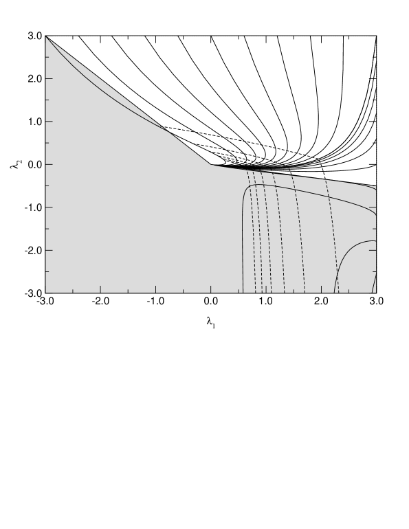
Figure 4: Renormalization group trajectories in the $\lambda_{1}$-$\lambda_{2}$ plane for $h(\Lambda_{TC})=3.5$. The solid curves are the trajectories, which begin at the boundary of the figure at $\mu=\Lambda_{TC}$. The dotted curves indicate $\mu=\Lambda_{TC}/2,\Lambda_{TC}/4,\dots$. In the shaded region, the vacuum is unstable.

In fig. 4, we display some typical renormalization group flows in the $\lambda_{1}-\lambda_{2}$ plane. We see that most of the trajectories which are stable in the ultraviolet remain stable as $\mu$ is reduced from $\Lambda_{TC}$ to $m_{s}$. The stability is fairly insensitive to the value of $h$ at the topcolor scale. If we consider all values of $\lambda_{1}$ and $\lambda_{2}$ with $|\lambda_{1,2}(\Lambda_{TC})|<10$, we find that about 65 percent of the renormalization group trajectories are stable over the range $\Lambda_{TC}>\mu>m_{s}$ for $h(\Lambda_{TC})=2$, 90 percent are stable for $h(\Lambda_{TC})=5$, and about 30 percent are stable for $h(\Lambda_{TC})=10$. If we restrict the values of $\lambda_{1,2}$ to $|\lambda_{1,2}(\Lambda_{TC})|<3$, the conclusions are qualitatively unchanged, except that there are fewer stable trajectories for $h(\Lambda_{TC})\raisebox{1.99997pt}{$\hbox to0.0pt{\raisebox{-5.0pt}{$\;\sim$}\hss}>\,$}9$.

We can use figure 4 to estimate the Higgs mass. In terms of $\lambda(\Lambda)$, we have

$$m_{\rm Higgs}^{2}=2\lambda(\Lambda)v^{2}\leq 2\lambda_{+}(\Lambda)v^{2}.$$ (5.72)

The surprising feature of figure 4 is that the values of $\lambda_{1,2}$ are very strongly focussed by renormalization group flow. As a result, we can make a qualitative estimate of the Higgs mass without detailed knowledge of the matching conditions at the topcolor scale. If we consider the region of parameter space $|\lambda_{1,2}(\Lambda_{TC})|<10$ and $h(\Lambda_{TC})\sim 2-10$, we find

$$\begin{array}[]{ccc}-0.4<\lambda_{1}(m_{s})<1.3,&-0.25<\lambda_{2}(m_{s})<0.35,&\lambda_{+}(m_{s})=\lambda_{1}(m_{s})+\lambda_{2}(m_{s})<1.1.\end{array}$$ (5.73)

Evolving the rest of the way down to $\mu=\Lambda$, we find $\lambda_{+}(\Lambda)\raisebox{1.99997pt}{$\hbox to0.0pt{\raisebox{-5.0pt}{$\;\sim$}\hss}<\,$}0.9$, and so

$$m_{\rm Higgs}\raisebox{1.99997pt}{$\hbox to0.0pt{\raisebox{-5.0pt}{$\;\sim$}\hss}<\,$}330~{}{\rm GeV}.$$ (5.74)

This is relatively light in comparison to typical topcolor models.

6 Conclusions

The singlet quarks discussed in section 3.3 will decay predominantly by GIM-violating interactions:

$$\chi\rightarrow cZ\,,sW^{+}\quad\quad\omega\rightarrow sZ\,,cW^{-}.$$ (6.75)

The bounds that we found in section 3.3 on the singlet masses apply only to the singlets that mix significantly with the left-handed doublets. At least one additional singlet is needed for anomaly cancellation in this model, and there are no strong indirect bounds on the masses of these non-mixing singlets. Presumably, their mixing will not be completely absent, and they will also decay by GIM violating processes to $W$s and $Z$s and the quarks with which they mix slightly, but with smaller widths. This rich quark phenomenology, possibly at quite accessible energies, is forced upon us by the constraints of anomaly cancellation in models like those of figure 1. In addition, in contrast to many topcolor models, we expect a relatively light Higgs. In this model, we also expect a large family of composite doublets, but these will appear only at the topcolor scale and may not be observable at the LHC.

7 Acknowledgments

We thank Markus Luty and John Terning for helpful discussions and to Sekhar Chivukula and Bogdan Dobrescu for comments on the manuscript.

Appendix A A toy model of flavor physics

To get some experience with flavor physics of this kind, we have undertaken a little demonstration project. We gauge the flavor symmetries in figure 2 with an $SO(3)$, and parameterize the mass terms from (2.10) and (2.11) and look at the masses that result to see whether we can get something that looks interesting. It will turn out that we cannot find the kind of hierarchical mass matrix that we need. A more elaborate scheme is needed, but we hope that some readers may find the exercise useful.

We consider a model with $N_{\cal U}=3\mathord{+}n_{\chi}$ charge $2/3$ quarks ${\cal U}_{R}^{m}$, $N_{\cal D}=3\mathord{+}n_{\omega}$ charge $-1/3$ quarks ${\cal D}_{R}^{m}$, and three $SU(2)$ doublets of quarks $\psi_{L}^{m}$, all of which feel the topcolor interaction. The ${\cal U}_{R}$ and ${\cal D}_{R}$ multiplets include both the standard model up and down quarks as well as the weak singlet $\chi$ and $\omega$ quarks. The composite Higgs fields are

$$H_{\cal U}^{m\overline{m}}=\overline{{\cal U}}_{R}^{\overline{m}}\psi_{L}^{m}$$ (A.76)

and

$$H_{\cal D}^{m\overline{m}}=\overline{{\cal D}}_{R}^{\overline{m}}\psi_{L}^{m}$$ (A.77)

In the absence of flavor-dependent couplings, and ignoring the weak $SU(2)\times U(1)$ interactions, the Higgs potential will have the form

$$V = -m^{2}(\mathop{\rm tr}H_{\cal U}^{\dagger}H_{\cal U}+\mathop{\rm tr}H_{\cal D}^{\dagger}H_{\cal D})+\lambda_{1}\mathop{\rm tr}\left[(H_{\cal U}^{\dagger}H_{\cal U})^{2}+(H_{\cal D}^{\dagger}H_{\cal D})^{2}+2H_{\cal U}^{\dagger}H_{\cal D}H_{\cal D}^{\dagger}H_{U}\right]$$ (A.78)

$$+ \lambda_{2}\left[(\mathop{\rm tr}H_{\cal U}^{\dagger}H_{\cal U})^{2}+(\mathop{\rm tr}H_{\cal D}^{\dagger}H_{\cal D})^{2}+2\mathop{\rm tr}(H_{\cal U}^{\dagger}H_{\cal U})\mathop{\rm tr}(H_{\cal D}^{\dagger}H_{\cal D})\right]\,.$$

This preserves the $SU(3)_{L}\times SU(N_{\cal U}\mathord{+}N_{\cal D})_{R}$ symmetry of the high-energy theory.

The degeneracy of the Higgs fields can be lifted by gauging an $SO(3)$ subgroup of the flavor symmetries. As a simple example, we place the three doublets into a triplet of $SO(3)$. We place the ${\cal U}$ and ${\cal D}$ quarks in representations of dimension $N_{\cal U}$ and $N_{\cal D}$. The Higgs bosons then live in product representations of $SO(3)$, which can be decomposed into representations of different total spin. If the $SO(3)$ is broken at a high scale (say 100 TeV or so), then in the low energy theory, single massive gauge boson exchange results in four-fermion operators of the form (2.13,2.14). These operators lift the degeneracy of Higgs fields with different total spin $J$. Writing the Higgs fields in terms of states of total $J$ using the Clebsch-Gordan decomposition,

$$\Phi^{JM}_{\cal Q}=\sum_{m\overline{m}}\langle JM|m\overline{m}\rangle H^{m\overline{m}}_{\cal Q}.$$ (A.79)

the Higgs mass terms have the form

$$V_{\rm Mass}=\sum_{JM}(m_{1}^{2}+\Delta_{J}m_{2}^{2})|\Phi^{JM}_{\cal U}|^{2}+\sum_{J^{\prime}M^{\prime}}(m_{1}^{2}+\Delta_{J^{\prime}}m_{2}^{2})|\Phi^{J^{\prime}M^{\prime}}_{\cal D}|^{2},$$ (A.80)

where

$$\Delta_{J}=\frac{1}{2}[J(J+1)-j_{{\cal Q}}(j_{{\cal Q}}+1)-j_{L}(j_{L}+1)].$$ (A.81)

We expect $m_{2}^{2}>0$, so that the states of lowest $J$ have the smallest masses and tend to condense more readily than those with higher $J$.

A further contribution to the Higgs potential comes from four-fermion operators that mix $\chi_{L}$ with ${\cal U}_{R}$ and $\omega_{L}$ with ${\cal D}_{R}$. These have the form

$$\frac{1}{M_{f}^{2}}\lambda^{\cal U}_{\overline{m}\alpha}(\overline{\chi}_{L}^{\alpha}\xi_{R})(\overline{\xi}_{L}{\cal U}_{R}^{\overline{m}})+\frac{1}{M_{f}^{2}}\lambda^{\cal U}_{\overline{m}\alpha}(\overline{\omega}_{L}^{\alpha}\xi_{R})(\overline{\xi}_{L}{\cal D}_{R}^{\overline{m}}),$$ (A.82)

where $M_{f}$ is the scale of flavor physics, of order 100 TeV or so. After the $\xi$ fields condense, these operators yield mass terms in the low energy:

$$\mu^{{\cal U}}_{\alpha\overline{m}}\overline{\chi_{L}}^{\alpha}{\cal U}_{R}^{\overline{m}}+\mu^{{\cal D}}_{\alpha\overline{m}}\overline{\omega_{L}}^{\alpha}{\cal D}_{R}^{\overline{m}}.$$ (A.83)

These operators break the $SU(N_{\cal U}+N_{\cal D})_{R}$ symmetry of the theory. This symmetry breaking should be reflected in some way by the Higgs potential. From the transformation properties of the symmetry breaking parameters $\mu^{\cal Q}$, we conclude that the symmetry breaking terms in the Higgs potential can be obtained by inserting factors of $(\mu^{{\cal Q},\dagger}\mu^{{\cal Q}})_{\overline{m}\overline{m}^{\prime}}$ at appropriate places in the Higgs potential. In particular, we expect terms of the form

$$\mathop{\rm tr}H^{\dagger}[\mu^{\dagger}\mu]H.$$ (A.84)

These terms lift the degeneracy of Higgs fields with different “magnetic” quantum number $M$.

We can also fix the sign of these $H^{\dagger}[\mu^{\dagger}\mu]H$ terms. In the limit that $\mu$ is large, some of the quarks become massive, and these masses must be reflected in the spectrum of composite scalars. As $\mu$ gets larger, the scalars must get heavier, and we conclude that the $H^{\dagger}[\mu^{\dagger}\mu]H$ contribution to the Higgs mass matrix must be positive. In the limit that $\mu$ is very small, this argument no longer works. However, we can include the effects of $\mu$ perturbatively to reach the same conclusion. Indeed, evaluating the correction to the composite scalar mass from Fig. 5, we find a contribution to the Higgs mass matrix of the form

$$\Delta m^{2}=\frac{h^{2}}{16\pi^{2}}\mu^{\dagger}\mu\log(\Lambda_{tc}^{2}/\overline{\mu}^{2}),$$ (A.85)

where $\overline{\mu}$ is a scale of order the typical singlet quark mass and $\Lambda_{tc}$ is the scale of the topcolor interactions. Hence in this limit we also find that the $H^{\dagger}[\mu^{\dagger}\mu]H$ terms give a positive contribution to the Higgs mass matrix.

..................................................................................................................................................................................................................................................................................................................................................................................................................................................................................................................................................................................................................................................................................................................................................................................................................$$\bullet \bullet \mu \mu^{\dagger}$$..................................................................................................................................   

Figure 5: The one-loop correction to the composite scalar mass with two insertions of $\mu$.

Now we would like to determine if this model gives a seesaw mass matrix for the quarks. This will depend on the relative “alignment” of $\mu$ and $\langle H\rangle$. The Yukawa couplings are

$$h\overline{\psi}_{L}H_{\cal U}{\cal U}_{R}+h\overline{\psi}_{L}H_{\cal D}{\cal D}_{R}.$$ (A.86)

After $SU(2)$ breaking, the quark mass matrix is

$$\left(\begin{array}[]{cc}\overline{u}^{m}_{L}\ \overline{\chi}^{\alpha}_{L}\end{array}\right)\left(\begin{array}[]{c}h\langle H^{m\overline{m}}\rangle\\ \mu_{\alpha\overline{m}}\end{array}\right)\left(\begin{array}[]{c}{{\cal U}_{R}^{\overline{m}}}\end{array}\right).$$ (A.87)

To obtain a seesaw mass matrix, we would like $\langle H\rangle$ to align with $\mu$ such that the largest entries of $\mu$ lie in the same column(s) as the largest entries of $\langle H\rangle$. Unfortunately, we find that this is not the case: the $\mu^{\dagger}\mu$ terms lift the masses of the Higgs fields such that the columns with the largest entries of $\mu$ also have the most positive masses, and so do not acquire large VEVs.

To illustrate this quantitatively, take the case $n_{\chi}=2$, $n_{\omega}=1$. For the parameters of the Higgs potential, take

$$\lambda_{1}=1,~{}\lambda_{2}=1,~{}m_{1}^{2}=1.37~{}{\rm TeV}^{2},~{}m_{2}^{2}=0.49~{}{\rm TeV}^{2}.$$ (A.88)

For this choice of masses, only the up-type Higgses with the lowest $J$ have negative mass-squared. For the singlet-quark mass-matrices, take (in TeV units)

$$\mu^{\cal U}=\left(\begin{array}[]{ccccc}0&0&0&2.4&3.6\\ 0&0&0.49&3.6&2.4\\ \end{array}\right),$$ (A.89)

and

$$\mu^{\cal D}=\left(\begin{array}[]{cccc}0&0&0&1\end{array}\right).$$ (A.90)

We include the effect of these masses on the Higgs potential by simply adding $\mu^{\dagger}\mu$ to the Higgs mass matrix. Minimizing the potential, we find that $\langle H_{\cal D}\rangle=0$, while

$$h\langle H_{\cal U}\rangle=\left(\begin{array}[]{ccccc}0&0&0.19&-0.05&0.03\\ 0&-0.33&0.05&-0.01&0\\ 0.46&-0.04&0.01&0&0\\ \end{array}\right)$$ (A.91)

We have used the Pagels-Stokar estimate of the Yukawa coupling $h$ with $\Lambda\sim 10\mu$, resulting in $h\simeq 3.4$. The Higgs VEV is mostly in the $J=1$, $M=-1$ direction, with small components on the $M=0,1$ directions. The resulting quark masses, in GeV, are

$$m^{\cal U}=\begin{array}[]{ccccc}195,&330,&460,&1230,&5940.\end{array}$$ (A.92)

The resulting spectrum does not have light quarks that could be identified with the first two generations, and does not yield a seesaw suppression of the top-quark mass. This result is generic over all of the parameter space.

References

- [1] For a nice recent review, see F. Wilczek, “Radical conservatism and nucleon decay,” hep-ph/0002045.
- [2] B. Holdom and J. Terning, “Large Corrections To Electroweak Parameters In Technicolor Theories,” Phys. Lett. B247, 88 (1990); M. Golden and L. Randall, “Radiative Corrections to Electroweak Parameters in Technicolor Theories,” Nucl. Phys. B361, 3 (1991); M. E. Peskin and T. Takeuchi, “A New Constraint On A Strongly Interacting Higgs Sector,” Phys. Rev. Lett. 65, 964 (1990); M. E. Peskin and T. Takeuchi, “Estimation of oblique electroweak corrections,” Phys. Rev. D46, 381 (1992).
- [3] C. T. Hill, Phys. Lett. B 266 (1991) 419.
- [4] D. B. Kaplan and H. Georgi, Phys. Lett. B136, 183 (1984); D. B. Kaplan, H. Georgi and S. Dimopoulos, Phys. Lett. B136, 187 (1984); H. Georgi, D. B. Kaplan and P. Galison, Phys. Lett. B143, 152 (1984).
- [5] S. Coleman and E. Weinberg, Phys. Rev. D7 (1973) 1888.
- [6] B. A. Dobrescu and C. T. Hill, Phys. Rev. Lett. 81, 2634 (1998) [hep-ph/9712319].
- [7] R. S. Chivukula, B. A. Dobrescu, H. Georgi and C. T. Hill, Phys. Rev. D59, 075003 (1999) [hep-ph/9809470].
- [8] H. Collins, A. Grant and H. Georgi, “Dynamically broken topcolor at large-N,” hep-ph/9907477.
- [9] H. Georgi, Nucl. Phys. B266 (1986) 274.
- [10] R. S. Chivukula, A. G. Cohen and E. H. Simmons, Phys. Lett. B380, 92 (1996) [hep-ph/9603311].
- [11] H. Pagels and S. Stokar, Phys. Rev. D20, 2947 (1979).
- [12] W. A. Bardeen, C. T. Hill and M. Lindner, “Minimal Dynamical Symmetry Breaking Of The Standard Model,” Phys. Rev. D41, 1647 (1990).
- [13] M. B. Popovic and E. H. Simmons, “Weak-singlet fermions: Models and constraints,” hep-ph/0001302.
- [14] C. Caso et al., “Review of particle physics,” Eur. Phys. J. C3, 1 (1998).
- [15] S. Weinberg, Physica A96, 327 (1979); A. Manohar and H. Georgi, Nucl. Phys. B234, 189 (1984); H. Georgi, Phys. Lett. B298 187 (1993) [hep-ph/9207278].
- [16] R. S. Chivukula, M. Golden and E. H. Simmons, “Critical constraints on chiral hierarchies,” Phys. Rev. Lett. 70, 1587 (1993) [hep-ph/9210276].
- [17] W. A. Bardeen, C. T. Hill and D. Jungnickel, “Chiral hierarchies, compositeness and the renormalization group,” Phys. Rev. D49, 1437 (1994) [hep-th/9307193].