Improved Unitarized Heavy Baryon Chiral Perturbation Theory for $\pi N$ Scattering

Abstract

We show how the unitarized description of pion nucleon scattering within Heavy Baryon Chiral Perturbation Theory can be considerably improved, by a suitable reordering of the expansion over the nucleon mass. Within this framework, the $\Delta$ resonance and its associated pole can be recovered from the chiral parameters obtained from low-energy determinations. In addition, we can obtain a good description of the six $S$ and $P$ wave phase shifts in terms of chiral parameters with a natural size and compatible with the Resonance Saturation Hypothesis.

PACS: 11.10.St;11.30.Rd; 11.80.Et; 13.75.Lb; 14.40.Cs; 14.40.Aq

Keywords: Chiral Perturbation Theory, Unitarity, $\pi N$-Scattering,

$\Delta$ Resonance, Heavy baryon, Partial waves.

I Introduction

The modern way to incorporate chiral symmetry and departures from it in low energy hadron dynamics, is by means of Chiral Perturbation Theory (ChPT)[2]. Being an effective Lagrangian approach all the detailed information on higher energies or underlying microscopic dynamics is effectively encoded in some low energy coefficients (LEC) which have to be determined experimentally. For processes involving only pseudoscalar mesons the expansion parameter is $p^{2}/(4\pi F)^{2}$ with $p$ their four momentum and $F$ the weak pion decay constant [2]. Of course, this expansion works better in the threshold region, breaking down at higher energies where the violation of unitarity becomes more and more severe. However, it has been shown that this applicability region can be extended by means of unitarization methods, describing remarkably well meson-meson scattering and its light resonances up to almost 1.2 GeV [3, 4]. In addition, it has been shown that the predicted unitarized amplitudes can reproduce the threshold region, and provide definite theoretical central values and error estimates of the phase-shifts away from threshold and up to about 1 GeV [5].

Baryons can also be included as explicit degrees of freedom if they are treated as heavy particles in a covariant framework [6] called Heavy-Baryon Chiral Perturbation Theory (HBChPT) [7, 8, 9]. In this case, the expansion to order $N=1,2,3,\dots$ is written in terms of contributions of the form $e^{N}/(F^{2l}M^{N+1-2l})$, where $l=1,\dots,[(N+1)/2]$, and $M$ is the baryon mass. The quantity $e$ is a generic parameter with dimensions of energy built up in terms of the pseudoscalar momenta and the velocity $v^{\mu}$ ($v^{2}=1$ ) and off-shellness $k$ of the baryons. The latter is defined from $p_{B}=\stackrel{{\scriptstyle\circ}}{{M}}v+k$, where $p_{B}$ and $\stackrel{{\scriptstyle\circ}}{{M}}$ are the baryon four momentum and its mass at lowest order in HBChPT, respectively.

Within HBChPT $\pi N$ scattering, has been calculated up to third order [11, 12] so far. In general, it is found that the HBChPT convergence is not as good as that of pure ChPT (see remarks in Ref. [11] and also below). Therefore, any attempt to unitarize this amplitude based on the increasing smallness of higher order terms, may formally reproduce HBChPT series but will likely fail numerically to describe the corresponding phase shifts even in the threshold region. Hence, any unitarization method should take into this slow convergence.

Unitarization methods have also been applied to $\pi N$ scattering in the literature. Already in the seventies Padé approximants had been used to unitarize simple phenomenological models [13], and a more systematic approach based on an effective Lagrangian formalism was called for. In addition, several relativistic phenomenological models exist which unitarize tree level amplitudes with the K-matrix method providing a reasonably good description of $\pi N$ scattering [14]. More recently, the $\Delta$ and $N^{*}$ resonances have also been considered as explicit degrees of freedom within HBChPT [15, 16, 17]. This requires the introduction of new parameters into the Chiral Lagrangian.

In contrast, the unitarization via the Inverse Amplitude Method (IAM) [3] does not introduce new parameters. However, when applied to $\pi N$ scattering [18], considering the higher orders to be increasingly small, the LEC turned out to be very different from those found within HBChPT [11] since they absorb higher order contributions which are not negligible. Nevertheless, in  [18] it was also shown that the $\Delta(1232)$ can be reproduced with the IAM using $O(p^{2})$ parameters constrained to lie within the range of values of Resonance Saturation, although the resulting $O(p^{3})$ parameters are still very unnatural. This situation is somewhat disappointing, since Padé approximants, which are similar to the IAM, together with simple phenomenological models, provided good descriptions of $\pi N$ scattering.

In this work we show how the $O(p^{3})$ HBChPT series can be reordered and the IAM modified, in order to i) implement exact unitarity , ii) comply with HBChPT at threshold and iii) describe the $\Delta$ resonance without introducing additional parameters.

II Partial Wave Amplitudes

Customarily, low-energy $\pi N$ scattering is described in terms of partial waves ( see, for instance Refs [19, 11]). We will rely heavily on the results in Ref. [11], where the third order HBChPT expressions where first obtained. However, in that work the full nucleon mass dependence has been retained, causing some order mixing. For our purposes, and in order to keep track of perturbative unitarity (see below), we have preferred to further expand the partial waves in terms of $1/M$ or $1/F^{2}$. That is, we only keep the pure $O(e/F^{2})$ (first order), $O(e^{2}/(F^{2}M))$ (second order) as well as the $O(e^{3}/F^{4})$ and $O(e^{3}/(F^{2}M^{2}))$ (third order) terms. One thus gets the following expansion,

$$f_{l\,\pm}^{\pm}=f_{l\,\pm}^{(1)\,\pm}+f_{l\,\pm}^{(2)\,\pm}+f_{l\,\pm}^{(3)\,\pm}+\cdots$$ (1)

which thus coincide with the first, second and third orders in [12], where the full nucleon mass dependence was not retained. However, we also separate these contributions in

$$f_{l\,\pm}^{(1)\,\pm} = {m\over F^{2}}t_{l\,\pm}^{(1,1)\,\pm}\Big{(}{\omega\over m}\Big{)}$$ (2)

$$f_{l\,\pm}^{(2)\,\pm} = {m^{2}\over F^{2}M}t_{l\,\pm}^{(1,2)\,\pm}\Big{(}{\omega\over m}\Big{)}$$ (3)

$$f_{l\,\pm}^{(3)\,\pm} = {m^{3}\over F^{4}}t_{l\,\pm}^{(3,3)\,\pm}\Big{(}{\omega\over m}\Big{)}+{m^{3}\over F^{2}M^{2}}t_{l\,\pm}^{(1,3)\,\pm}\Big{(}{\omega\over m}\Big{)}$$ (4)

where $t^{(n,m)\,\pm}_{l\,\pm}$ are dimensionless functions of the dimensionless variable $\omega/m$, independent of $F,M$ and $m$. The analytical expressions are too long to be displayed here, but can be easily obtained starting from Ref. [11]. The convenience of the double superscript notation will be explained below; $n+1$ indicates the power in $1/F$ and $m$ the total order in the HBChPT counting. The unitarity condition ${\rm Im}f_{l\,\pm}^{-1}=-q$ becomes in perturbation theory

$${\rm Im}\,t_{l\,\pm}^{(1,1)\,\pm}={\rm Im}\,t_{l\,\pm}^{(1,2)\,\pm} = {\rm Im}\,t_{l\,\pm}^{(1,3)\,\pm}=0$$ (5)

$${\rm Im}\,t_{l\,\pm}^{(3,3)\,\pm} = {q\over m}|t_{l\,\pm}^{(1,1)\,\pm}|^{2}$$ (6)

The equivalent of the last equation above for the $f$ amplitudes is not satisfied exactly if the nucleon mass dependence is retained through a redefinition of the nucleon field as in Ref.( [11]) (see, for instance, comments in [12] and [18]), although, of course, the corrections are just higher order in HBChPT. These exact relations for the perturbative contributions will be very convenient later on, and, as we have commented above, that is the reason why we have preferred to expand the amplitudes as in Eq. (1).

The scattering lengths $a_{l,\pm}^{\pm}$ and effective ranges $b_{l,\pm}^{\pm}$ are defined by

$${\rm Re}f_{l,\pm}^{\pm}=q^{2l}\Big{(}a_{l,\pm}^{\pm}+q^{2}b_{l,\pm}^{\pm}+\cdots\Big{)}$$ (7)

Obviously, the expansion of Eq. (4) carries over to the threshold parameters, $a_{l,\pm}^{\pm}$ and $b_{l,\pm}^{\pm}$, which we will use next to illustrate the slow low energy convergence of the HBChPT series.

Throughout this paper we use $F=92.4\,{\rm MeV}$, $M=938.27\,{\rm MeV}$, $m=139.57\,{\rm MeV}$ and $g_{A}=1.26$. Concerning the LEC , there are several determinations: The first one, which we give as Set I in Table I, was obtained from a fit to the extrapolated threshold parameters $a_{0,+}^{\pm}$, $b_{0,+}^{\pm}$, $a_{1,\pm}^{\pm}$, the Goldberger-Treiman discrepancy and the nucleon $\sigma-$term  [11]. Note that the full nucleon mass dependence was retained. For our purposes it is thus more convenient a more recent determination[12] from a low energy fit to $\pi N$ phase-shift data, although the authors used a different notation for the chiral parameters. The resulting LEC translated to the $a_{i}$ and $b_{i}$ notation (see [20, 12] ) are given in the Set II of Table I. On the theoretical side, there are estimations of the $a_{i}$ parameters assuming they are saturated by the exchange of resonances [10], in fairly good agreement with experimental determinations.

III Low Energy Convergence

In all our following considerations we further expand the amplitudes and threshold parameters as in Eqs.(4). For the scattering lengths we thus have

$$a_{2I\,2J}^{l}m^{2l+1}={m\over F^{2}}\alpha^{(1,1)}+{m^{2}\over F^{2}M}\alpha^{(1,2)}+{m^{3}\over F^{2}M^{2}}\alpha^{(1,3)}+{m^{3}\over F^{4}}\alpha^{(3,3)}+\cdots$$ (8)

and a similar expression for $b_{2I\,2J}^{l}m^{2l+3}$. The slower convergence of the HBChPT series as compared with ChPT was pointed out by the authors of the first calculations, (see for instance the comments in [10, 11, 12]). For our purposes, we have found instructive to separate the contributions to the scattering lengths and effective ranges of the lowest partial waves, which are given in Table II, using the set II of LEC in Table I. Note that, in this way, the threshold parameters are predictions, unlike those from set I which uses them as an input. A distinctive pattern emerging from this Table is that the contribution of order $1/(F^{2}M^{2})$ is always rather small. Only in some cases, however, is the contribution of order $1/F^{4}$ also small. This is so in the $P_{33}$ channel in particular, which is the one less likely to be well described by HBChPT alone due to the low mass of the $\Delta(1232)$ resonance. Hence, it seems that close to threshold the $1/F^{2}$ expansion converges faster than the $1/M$ expansion. Actually, the $1/F^{2}$ and $1/(F^{2}M)$ terms are comparable. It is clear that any unitarization method will only be consistent with the HBChPT approach, if it treats both the first and the second order as equally important.

IV Unitarization method for the reordered series

Our unitarization method assumes that, as suggested by the perturbative calculation, the chiral expansion in terms of $1/F^{2}$ converges much faster than the finite nucleon mass $1/M$ corrections. Indeed there are some recent theoretical attempts[23, 24] to define a relativistic power counting not requiring the heavy baryon idea, returning somehow to the spirit of older relativistic studies [25]. As a matter of fact, we show that the well-known IAM approach applied to the reordered HBChPT series generates the $P_{33}$ phase-shift satisfactorily, just using the LEC determined at low energies. In addition, it is possible to improve the overall description of the six $\pi N$ scattering S and P waves, using those very same parameters. Finally, if one fits the $\pi N$ phase shifts with this method (either constraining the parameters to the Resonance Saturation Hypothesis or leaving all the parameters unconstrained) the resulting parameters have a much more natural size, and the $\chi^{2}$ per d.o.f is considerably better than those obtained with the IAM applied to plain HBChPT [18].

	M.Mojzis [11]	N.Fettes et al. [12]	Resonance Saturation fit	Unconstrained fit
	Set I	Set II	Set III	Set IV
$a_{1}$	$-$ 2.60 $\pm$ 0.03	$-$ 2.69 $\pm$ 0.4	$-$2.065 $\pm$ 0.007	$-$ 1.36 $\pm$ 0.02
$a_{2}$	1.40 $\pm$ 0.05	1.34$\pm$0.1	0.915$\pm$0.005	0.438$\pm$0.015
$a_{3}$	$-$1.00 $\pm$ 0.06	$-$1.15$\pm$0.1	$-$0.85 (input)	$-$0.70$\pm$0.04
$a_{5}$	3.30$\pm$0.05	3.1$\pm$0.5	2.700$\pm$0.001	1.29$\pm$0.04
$\tilde{b}_{1}+\tilde{b}_{2}$	2.40$\pm$0.3	2.60$\pm$0.2	3.95$\pm$0.04	3.06$\pm$0.3
$\tilde{b}_{3}$	$-$2.8$\pm$0.6	$-$3.96$\pm$0.9	-1.45$\pm$0.03	$-$0.41$\pm$0.27
$\tilde{b}_{6}$	1.4$\pm$0.3	0.55$\pm$0.5	$-$1.17$\pm$0.17	$-$1.5$\pm$0.2
$b_{16}-\tilde{b}_{15}$	6.1$\pm$0.6	7.1 $\pm$0.5	5.86 $\pm$0.19	7.4 $\pm$0.5
$b_{19}$	$-$2.4$\pm$0.4	$-$1.72$\pm$0.3	-0.44$\pm$0.21	$-$3.7$\pm$0.2

TABLE I.: HBChPT low energy constants. Those in the first column were obtained from fitting the extrapolated threshold parameters $a_{0,+}^{\pm}$, $b_{0,+}^{\pm}$, $a_{1,\pm}^{\pm}$, the Goldberger-Treiman discrepancy and the nucleon $\sigma-$term to the HBChPT predictions [11]. In the second column we give the parameters obtained from a low energy fit to $\pi N$ phase-shift data [12]. In the third column we give the parameters obtained from an IAM fit with the $a_{i}$ constrained to the ranges predicted by resonance saturation. Finally, the fourth column is the result of a totally unconstrained fit.

	$1/F^{2}$	$1/(F^{2}M)$	$1/(F^{2}M^{2})$	$1/F^{4}$	Total	SP98	KA85
$a_{3\,1}^{0}$	$-$0.65	$-$0.04	+0.07	$+$0.07	$-$0.55${}^{+0.16}_{-0.18}$	$-$0.64 $\pm$ 0.01	$-$0.72
$a_{1,1}^{0}$	1.3	$-$0.34	$-$0.08	0.07	0.94$\pm$0.23	1.27 $\pm$ 0.02	1.26
$a_{3\,3}^{1}$	35.3	47.95	$-$1.75	0.26	81.8${}^{+0.8}_{-0.9}$	80.3$\pm$0.6	78.75
$a_{1\,3}^{1}$	$-$17.7	15.46	$-$3.1	$-$6.35	$-$11.66$\pm 0.9$	$-$10.5 $\pm$ 0.9	$-$11.00
$a_{3\,1}^{1}$	$-$17.7	12.96	$-$1.84	$-$9.77	$-$16.3${}^{+1.0}_{-0.9}$	$-$15.9 $\pm$ 1.0	$-$16.19
$a_{1\,1}^{1}$	$-$70.7	85.6	$-$3.77	$-$46.13	$-$35.0${}^{+1.6}_{-1.5}$	$-$27.0 $\pm$1.4	$-$28.67

TABLE II.: HBChPT, lowest partial S and P wave- scattering lengths, $a_{2I\,2J}^{l}$ (in ${\rm GeV}^{-2l-1}$ units) for $\pi N$ scattering using set II in Table I, decomposed as a sum of terms of first order $1/F^{2}$, second order, $1/(F^{2}M)$, and third order, $1/(F^{2}M^{2})$ and $1/(F^{4})$. The sum of all the terms yields the total scattering length parameter. For brevity, we only quote the errors in the final sum. The experimental values come from Ref. [22] for SP98, and Ref. [21] for KA85. For very recent and accurate values of only the S-wave scattering lengths see [28]

The IAM is based on the fact that elastic unitarity imposes the following relation on a generic partial wave $f$ and its inverse $f^{-1}$ (we drop the $l$, $I$ and $J$ labels for simplicity):

$${\rm Im}\,f=q\,|f|^{2}\quad\Rightarrow\quad{\rm Im}\,f^{-1}=-q$$ (9)

As a consequence, any amplitude satisfying exactly elastic unitarity has the form

$$f=\frac{1}{{\rm Re}\,f^{-1}-i\,q}$$ (10)

Thus, we only have to calculate ${\rm Re}\,f^{-1}$, whose different approximations provide different unitarization methods. Here we consider its expansion in terms of $m^{2}/F^{2}$, i.e.

$$f(\omega,m,F,M)={m\over F^{2}}t^{(1)}(\omega/m\,,\,m/M)+{m^{3}\over F^{4}}t^{(3)}(\omega/m\,,\,m/M)+\dots$$ (11)

where we have used that $t^{(2n+1)}$ are dimensionless functions, only depending on dimensionless variables. The functions $t^{(1)}$ and $t^{(3)}$ are only known in a further $m/M$ expansion,

$$t^{(2n+1)}(\omega/m,m/M)=t^{(2n+1,2n+1)}(\omega/m)+{m\over M}\,t^{(2n+1,2n+2)}(\omega/m)+\,\left({m\over M}\right)^{2}\,t^{(2n+1,2n+3)}(\omega/m)\,\dots$$ (12)

yielding Eq. (1) and Eq. (4) after a suitable isospin projection.

Perturbative unitarity in this expansion requires,

$${\rm Im}\,t^{(1)}=0\quad,\quad{\rm Im}\,t^{(3)}={q\over m}|t^{(1)}|^{2},$$ (13)

which also imply an infinite conditions in the $1/M$ expansion. For $f^{-1}$ we get then

$${1\over f}={F^{2}\over m}{1\over t^{(1)}}-m{t^{(3)}\over[t^{(1)}]^{2}}+\dots$$ (14)

Obviously, expanding in $m/F^{2}$ may be justified provided these corrections are small. As we have shown, for the $P_{33}$ channel, they are small precisely at threshold, and there the unitarization scheme will, approximately, reproduce the perturbative result. At the same time, unitarity is exactly implemented since, thanks to eqs.(13) the above formula is of the form given in eq.(10). However, the $1/M$ terms are not small corrections at threshold, and thus we do not further “expand the denominator”. In this way we keep the first mass corrections as equally important. At present, only the $t^{(1,1)}$, $t^{(1,2)}$, $t^{(1,3)}$ and $t^{(3,3)}$ HBChPT terms are known (see our previous footnote ∥ ‣ I). Therefore, we do not know neither $t^{(3,4)}$ nor $t^{(3,5)}$. i.e $O(1/(F^{4}M))$ and $O(1/(F^{4}M^{2}))$ respectively, and we can only approximate the numerator of the second term by $t^{(3)}\simeq t^{(3,3)}$. That is, we know the first three orders of the denominator $1/m$ expansion, but not their counterparts in the numerator. Therefore, although we could use $t^{(1)}\simeq t^{(1,1)}+t^{(1,2)}+t^{(1,3)}$ in the denominator, for consistency with the numerator expansion we keep only $t^{(1)}\simeq t^{(1,1)}$. Incidentally, this corresponds to the static limit of the second term. Note also that strict unitarity is still satisfied. Of course, it would be desirable to compute at least $t^{(3,4)}$ and $t^{(3,5)}$ in order to be able to keep also $t^{(1,2)}$ in the denominator of the second term of the mentioned equation. After these remarks, we have

$${1\over f|_{\rm Unitarized}}={F^{2}\over m}{1\over t^{(1,1)}+{m\over M}\,t^{(1,2)}+\,({m\over M})^{2}\,t^{(1,3)}}-m{t^{(3,3)}\over[t^{(1,1)}]^{2}}$$ (15)

At threshold, our formula yields a modified scattering length

$${1\over a_{\rm Unitarized}} = {F^{2}\over m}{1\over\alpha^{(1,1)}+{m\over M}\,\alpha^{(1,2)}+\,({m\over M})^{2}\,\alpha^{(1,3)}}-m{\alpha^{(3,3)}\over[\alpha^{(1,1)}]^{2}}$$ (16)

$$= {1\over a_{\rm HBChPT}-({m^{3}\over f^{4}})\,\alpha^{(3,3)}}-m{\alpha^{(3,3)}\over[\alpha^{(1,1)}]^{2}}$$ (17)

which, using set II in Table I, yields $a_{3\,3}^{1}|_{\rm Unitarized}=82.95{}^{+0.34}_{-0.35}{\rm GeV}^{-3}$, to be compared with $a_{3\,3}^{1}|_{\rm HBChPT}=81.8{}^{+0.8}_{-0.9}{\rm GeV}^{-3}$, both compatible with the experimental values. Notice that if we had expanded the denominator considering the second order contribution $O(1/(F^{2}M))$ to be small we would have obtained strictly the IAM method as used in Ref. [18],

$${1\over a_{\rm IAM}}={F^{2}\over m}\left\{{1\over\alpha^{(1,1)}}-{m\over M}\,{\alpha^{(1,2)}\over[\alpha^{(1,1)}]^{2}}-\left({m\over M}\right)^{2}\,{\alpha^{(1,3)}\over[\alpha^{(1,1)}]^{2}}+\left({m\over M}\right)^{2}\,{[\alpha^{(1,2)}]^{2}\over[\alpha^{(1,1)}]^{3}}\right\}-m{\alpha^{(3,3)}\over[\alpha^{(1,1)}]^{2}}$$ (18)

yielding $a_{3\,3}^{1}|_{\rm IAM}=22.8{\rm GeV}^{-3}$. This explains why an unconstrained IAM fit with standard HBChPT leads to LEC which are so different from those found in [11], as noted in Ref. [18].

V Numerical Results

From our previous discussion it is clear that at threshold our unitarized amplitude will reproduce very accurately and within error bars the HBChPT results and hence the experimental data. In addition, we expect that the $P_{33}$ phase shift can be extended up to the resonance region by propagating the errors of the LEC. It is also tempting to extend the other five $S$ and $P$ wave phase shifts. We show in Fig.1 the phase shifts obtained from our unitarization method, Eq. (15), compared with the experimental $\pi N$ data [22]. The shaded area corresponds to the phase shifts obtained by propagating the errors of the parameters given in Ref.[12] (See Table I, set II) by means of a Monte Carlo gaussian sampling of the LEC for any given CM energy value. Only for comparison, the dotted line corresponds to standard HBChPT extrapolated to high energies.

As one can see from the figures, the prediction of our unitarized approach produces a distinctive resonance in the $P_{33}$ channel, with very similar parameters to the physical $\Delta$ as we will see below. Concerning the other channels, there is some improvement in the $S$ waves, and a worse behavior for the $P_{13}$, $P_{31}$ and $P_{11}$, but note that these three partial waves have very tiny phase shifts, and any small error yields a large relative deviation.

The mass and width of the $\Delta$ resonance can be obtained either from the phase shifts, by means of $\delta^{1}_{33}|_{s=M_{\Delta}^{2}}=\pi/2$ and $1/\Gamma_{\Delta}=M_{\Delta}(d\delta^{1}_{33}/ds)|_{s=M^{2}_{\Delta}}$, or from its associated pole in the

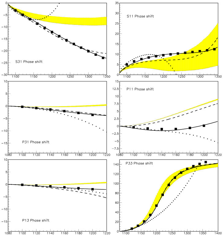
FIG. 1.: Phase shifts as a function of the total CM energy $\sqrt{s}$. Experimental data are from Ref. [22]. The shaded areas correspond to the propagated errors of the parameters in set II, which were obtained from low-energy data. The dotted line is the HBChPT result extrapolated to high energies. The dashed line is a fit with our unitarization procedure constrained to Resonance Saturation, whereas the continuous line corresponds to an unconstrained fit.

second Riemann sheet ($\sqrt{s_{pole}}\simeq M_{\Delta}-i\Gamma_{\Delta}/2$). We give in Table III the results for different parameter sets. Note that the width of the “predicted” resonance from the parameters determined from low-energy data (set II) is qualitatively very similar to the real $\Delta$. Of course, once we fit to the data (set III and IV), we obtain a much better description.

However, it was pointed out in Ref.[18] that the direct fit using the IAM directly on the HBChPT series leads to chiral parameters of very unnatural size. That is not the case when we fit with the reordered method proposed here as it can be seen in set IV of table I. This set comes from an unconstrained fit to the six $S$ and $P$ wave $\pi N$ phase shifts, which is represented as a continuous line in Fig.1. For the fits, which start at 1130 MeV, we have used the MINUIT minimization routine assigning a 3% uncertainty as in [12] plus a systematic error of one degree to the data in [22] (similar treatments are followed in [17, 18]).

Much more interesting [18] are those fits where the $O(p^{2})$ parameters are constrained to the range estimated by the Resonance Saturation Hypothesis [10]. The fitted parameters are given as set III in Table I, and the result is represented as the dashed line in Fig.1. In this case the $P_{11}$ and $S_{11}$ are not so well described, which may be due to effects of the $N^{*}(1440)$ and $N(1535)$, respectively, which are the closest resonances to the energy regions displayed in Fig.1. Indeed, the former plays a marginal role in the Resonance Saturation Hypothesis whereas the latter is not even considered.

A particularly relevant feature of these fits is that not only the resulting parameters have a more natural size, but also the $\chi^{2}$ per d.o.f. is between three and four times smaller than for the corresponding IAM fit applied to the standard HBChPT ordering. From this we can conclude that considering the $1/M$ expansion separately as in our formalism is a sensible approach, apart from the details of its precise realization.

FIG. 2.: $P_{33}$ phase shift. The upper shaded area corresponds to the result of propagating the errors of the set I parameters. This illustrates the uncertainties due to the choice of parameter sets from the literature. The intermediate shaded area cover the propagated uncertainties of set II if we applied the IAM in the static limit. Finally, with the same set we show, in the lowest shaded area the result of the IAM when applied directly to the standard HBChPT expansion.

	set I	set II	set III	set IV	PDG [26]
$M_{\Delta}$ (MeV)	1240 ${}^{+23}_{-17}$	1222 ${}^{+15}_{-12}$	1227 $\pm 4$	1226${}^{+14}_{-12}$	1230 - 1234
$\Gamma_{\Delta}$ (MeV)	157${}^{+46}_{-33}$	117${}^{+24}_{-18}$	104.1 ${}^{+5.2}_{-4.4}$	107${}^{+21}_{-16}$	115-125
Re (pole position) (MeV)	1205	1204	1204	1204	1209-1211
$\Gamma$ -2 Im (pole position) (MeV)	110	110	110	84	98-102

TABLE III.: $\Delta$ resonance parameters. The two first rows are obtained from the condition $\delta^{1}_{33}|_{s=M_{\Delta}^{2}}=\pi/2$ and $1/\Gamma_{\Delta}=M_{\Delta}(d\delta^{1}_{33}/ds)|_{s=M^{2}_{\Delta}}$. The second two rows are the real part and minus twice the imaginary part of its associated pole position, calculated for the central values of each set (the errors are expected to be of the same order than for the first two columns).

As an illustration of the uncertainties due to the different determinations of chiral parameters, we have also shown in Fig.2 the area corresponding to our formula applied to set I. We reobtain the same qualitative result, although numerically the mass and width of the $\Delta$ are worse than those obtained with set II. In addition, in order to estimate the convergence rate of our calculation, we have also plotted in Fig.2 the prediction in the static limit ($M\to\infty$). The shaded area in Fig.2 corresponds to the propagated errors of the parameter set II in this limit. As we see, there is also a distinctive resonant behavior, so that the bulk of the dynamics is contained in the static limit. However, the finite mass corrections, particularly the $1/(F^{2}M)$ contribution, are important to achieve a better description.

We have also studied what happens if one includes the incomplete higher order contributions to the second quotient in Eq. (14), i.e. if one approximates $t^{(1)}\simeq t^{(1,1)}+t^{(1,2)}+t^{(1,3)}$ in its denominator. In such case we obtain a worse result, closer to that of the static limit, but still there is a distinctive resonant behavior, improving the IAM results with the standard HBChPT expansion. This suggests that the unknown higher order contributions (see footnote ∥ ‣ I) in the numerator could give rise to some cancellation with those still incomplete of the denominator. Finally, we also show in Fig.2 the results obtained within the conventional IAM approach, for the parameter set II. As it was already pointed out in [18] the result is extremely poor if one uses the parameters determined from low energy data.

VI Conclusions and Outlook

Heavy Baryon Chiral Perturbation Theory provides definite predictions for the $\pi N$ scattering amplitudes in the threshold region. However it violates exact unitarity if the perturbative expansion is truncated to some finite order and also is unable to describe the $\Delta$ resonance (and its associated pole) in the $P_{33}$ channel. The analysis up to third order shows that the leading finite nucleon mass correction, which is second order, is of comparable size to the static approximation and in fact it dominates the corrections at threshold. This suggests a unitarization method using the expansion in inverse powers of the weak pion decay constant but without making the heavy baryon expansion. Such an idea is supported by recent theoretical attempts to redefine a relativistic chiral counting for baryons. We have proposed a unitarization scheme based on the Inverse Amplitude Method applied to this reordered HBChPT expansion. It provides a prediction for the $\pi N$ phase shifts, which generates a $\Delta$ resonance from the low energy constants and their errors, as determined from HBChPT. The fits within this scheme provide chiral parameters of a natural size and a better overall description than those performed with the IAM applied to the HBChPT standard expansion. This result suggests that including the $1/M$ expansion separately is a sensible physical approach. In addition, this method can be easily generalized to higher orders and coupled channels. Further work along these lines is in progress.

REFERENCES

- [1]
- [2] J. Gasser and H. Leutwyler, Ann. of Phys., (N.Y.) 158 (1984) 142.
- [3] T. N. Truong, Phys. Rev. Lett. 661 (1988) 2526; Phys. Rev. Lett. 67 (1991) 2260; A. Dobado, M.J.Herrero and T.N. Truong, Phys. Lett. B235 (1990) 134 ; A. Dobado and J.R. Peláez,Phys. Rev. D47 4883 (1993); Phys. Rev.D56 (1997) 3057.
- [4] J.A. Oller, E. Oset and J.R. Peláez, Phys. Rev. Lett. 80 (1998) 3452 ; Phys. Rev. D59 (1999) 074001; hep-ph/9909556. F. Guerrero and J. A. Oller, Nucl. Phys. B537 (1999) 459.
- [5] J. Nieves and E. Ruiz Arriola, Phys. Lett. B455 (1999) 30; hep-ph/9907469 and references therein.
- [6] N. Isgur and M.B. Wise, Phys. Lett. B232 (1989) 113.
- [7] E. Jenkins and A. V. Manohar, Phys. Lett. B255 (1991) 558.
- [8] V. Bernard, N. Kaiser, J. Kambor and U. -G. Meißner, Nucl. Phys. B388 (1992) 315.
- [9] For a review see e.g. V. Bernard, N. Kaiser and U.-G. Meißner, Int. J. Mod. Phys. E4 (1995) 193 and references therein.
- [10] V. Bernard, N. Kaiser and U.-G. Meißner, Nucl. Phys. A615 (1997) 483.
- [11] M. Mojzis, Eur. Phys. Jour. C2 (1998) 181.
- [12] N. Fettes, U.-G. Meißner and S. Steininger, Nucl.Phys. A640 (1998) 199.
- [13] J.L. Basdevant, Fort. der Phys. 20 (1972) 283.
- [14] M. G. Olsson and E. T. Osypowski, Nucl. Phys. B101 (1975) 136. D. Bofinger and W. S. Woolcock, Nuovo Cimento A104 (1991) 655. F. Gross and Y. Surya, Phys. Rev C47 (1993) 703. P.F.A. Goudsmit et al., Nucl. Phys. A575 (1994) 673.
- [15] A. Datta and S. Pakvasa, Phys. Rev. D56 (1997). P. J. Ellis and H.-B. Tang, Phys. Rev. C56 (1997) 3363 ; C57 (1998) 3356.
- [16] T. R. Hemmert, B. R. Holstein and J. Kambor, Phys. Lett. B395 (1997).
- [17] U. -G. Meißner and J. A. Oller, nucl-th/9912026.
- [18] A. Gomez-Nicola and J. R. Peláez, hep-ph/9912512 (To appear in Phys. Rev. D.) and hep-ph/9909568.
- [19] T. Ericson and W. Weise, Pions and Nuclei, Clarendon Press, Oxford, 1988.
- [20] G.Ecker and M.Mojzis, Phys.Lett. B365 (1996) 312-318.
- [21] R. Koch, Nucl. Phys. A348 (1986) 707.
- [22] R.A. Arndt, I.I. Strakovsky, R.L. Workman, and M.M. Pavan, Phys. Rev. C52, 2120 (1995). R. Arndt et al. nucl-th/9807087. SAID online-program.(Virginia Tech Partial-Wave Analysis Facility). Latest update, http://said.phys.vt.edu.
- [23] T. Becher and H. Leutwyler, hep-ph/9901384.
- [24] J.Gegelia, G. Japaridze and X. Q. Wang, hep-ph/9910260.
- [25] J. Gasser, M.E. Sainio and A. Svarc, Nucl. Phys. B307 (1988) 779.
- [26] Review of Particle Physics, Eur. Phys. J C 3 (1998) 1.
- [27] N. Fettes and U-G. Meißner, hep-ph/0002162.
- [28] H.-Ch.Schroeder et al., Phys. Lett. B 469 (1999) 25.