SLAC-PUB-8436 June 2000

Experimental Probes of Localized Gravity:
On and Off the Wall

H. Davoudiasl, J.L. Hewett, and T.G. Rizzo
Stanford Linear Accelerator Center

Stanford CA 94309, USA

The phenomenology of the Randall-Sundrum model of localized gravity is analyzed in detail for the two scenarios where the Standard Model (SM) gauge and matter fields are either confined to a TeV scale 3-brane or may propagate in a slice of five dimensional anti-deSitter space. In the latter instance, we derive the interactions of the graviton, gauge, and fermion Kaluza-Klein (KK) states. The resulting phenomenological signatures are shown to be highly dependent on the value of the 5-dimensional fermion mass and differ substantially from the case where the SM fields lie on the TeV-brane. In both scenarios, we examine the collider signatures for direct production of the graviton and gauge KK towers as well as their induced contributions to precision electroweak observables. These direct and indirect signatures are found to play a complementary role in the exploration of the model parameter space. In the case where the SM field content resides on the TeV-brane, we show that the LHC can probe the full parameter space and hence will either discover or exclude this model if the scale of electroweak physics on the 3-brane is less than 10 TeV. We also show that spontaneous electroweak symmetry breaking of the SM must take place on the TeV-brane.

1 Introduction

A novel approach which exploits the geometry of extra spacetime dimensions has been recently proposed[1, 2, 3] as a means to resolving the hierarchy problem. In one such scenario due to Arkani-Hamed, Dimopoulos, and Dvali (ADD)[1], the apparent hierarchy is generated by a large volume for the extra dimensions. In this case, the fundamental Planck scale in $4+n$-dimensions, $M$, can be brought down to a TeV and is related to the observed 4-d Planck scale through the volume $V_{n}$ of the compactified dimensions, $M^{2}_{Pl}=V_{n}M^{2+n}$. In an alternative scenario due to Randall and Sundrum (RS)[2], the observed hierarchy is created by an exponential warp factor which arises from a 5-dimensional non-factorizable geometry. An exciting feature of these approaches is that they both afford concrete and distinctive phenomenological tests[4, 5]. Furthermore, if these theories truly describe the source of the observed hierarchy, then their signatures should appear in experiment at the TeV scale.

The purpose of this paper is to explore the detailed phenomenology that arises in the non-factorizable geometry of the RS model. We will examine the cases where the Standard Model (SM) gauge and matter fields can propagate in the additional spacial dimension, denoted as the bulk, as well as being confined to ordinary 3+1 dimensional spacetime. The broad phenomenological features of the latter case were spelled out in Ref. [5]. Here, we expand on this previous work by considering the effects in precision electroweak observables and investigating a wider range of collider signatures, including the case of lighter graviton Kaluza-Klein (KK) excitations. We also show that the LHC can probe the full parameter space of this model and hence will either discover or exclude it if the scale of electroweak physics on the 3-brane is less than 10 TeV. The experimental signatures of the former scenario, where the SM fields reside in the bulk, are considered here for the first time. As we will see below, this possibility introduces an additional parameter, given by the 5-dimensional mass of the fermion fields, which has a dramatic influence on the phenomenological consequences and yields a range of experimental characteristics. While the general features of these signatures remain indicative of this type of geometry, the various details of the different cases can be taken to represent a wide class of possible models similar in nature to the RS scenario. We also present an argument which shows that spontaneous electroweak symmetry breaking must be confined to the Standard Model 3-brane.

The Randall-Sundrum model consists of a 5-dimensional non-factorizable geometry based on a slice of AdS₅ space with length $\pi r_{c}$, where $r_{c}$ denotes the compactification radius. Two 3-branes, with equal and opposite tensions, rigidly reside at $S_{1}/Z_{2}$ orbifold fixed points at the boundaries of the AdS₅ slice, taken to be $y=r_{c}\phi=0,r_{c}\pi$. The 5-dimensional Einstein’s equations permit a solution which preserves 4-dimensional Poincaré invariance with the metric

$$ds^{2}=e^{-2\sigma(\phi)}\eta_{\mu\nu}dx^{\mu}dx^{\nu}-r_{c}^{2}d\phi^{2}\,,$$ (1)

where the Greek indices extend over ordinary 4-d spacetime and $\sigma(\phi)=kr_{c}|\phi|$. Here $k$ is the AdS₅ curvature scale which is of order the Planck scale and is determined by the bulk cosmological constant $\Lambda=-24M_{5}^{3}k^{2}$, where $M_{5}$ is the 5-dimensional Planck scale. The 5-d curvature scalar is then given by $R_{5}=-20k^{2}$. Examination of the action in the 4-d effective theory yields the relation

$$\overline{M}_{Pl}^{2}={M_{5}^{3}\over k}(1-e^{-2kr_{c}\pi})$$ (2)

for the reduced 4-d Planck scale. The scale of physical phenomena as realized by the 4-d flat metric transverse to the 5th dimension $y=r_{c}\phi$ is specified by the exponential warp factor. TeV scales can naturally be attained on the 3-brane at $\phi=\pi$ if gravity is localized on the Planck brane at $\phi=0$ and $kr_{c}\simeq 11-12$. The scale of physical processes on this TeV-brane is then $\Lambda_{\pi}\equiv\overline{M}_{Pl}e^{-kr_{c}\pi}$. The observed hierarchy is thus generated by a geometrical exponential factor and no other additional large hierarchies appear. It has been demonstrated[6] that this value of $kr_{c}$ can be stabilized without the fine tuning of parameters by minimizing the potential for the modulus field, or radion, which describes the relative motion of the 2 branes. In the original construction of the RS model utilizing this stabilization mechanism, gravity and the modulus stabilization field may propagate freely throughout the bulk, while the SM fields are assumed to be confined to the TeV (or SM) brane at $\phi=\pi$. The 4-d phenomenology of this model is governed by only two parameters[5], given by the curvature $k$ and $\Lambda_{\pi}$. The radion, which receives a mass during the stabilization procedure, is expected to be the lightest new state and admits an interesting phenomenology[7] which we will not consider here.

This scenario has enjoyed immense popularity in the recent literature, with the cosmological/astrophysical [8], string theoretic[9], and phenomenological implications all being explored. We note that similar geometrical configurations have previously been found to arise in M/string theory[10]. In addition, extensions of this scenario where the higher dimensional space is non-compact[11], i.e., $r_{c}\rightarrow\infty$, as well as the inclusion of additional spacetime dimensions and branes[12] have been discussed.

Given the success of the RS scenario, it is logical to ask if it can be extended to include other fields in the bulk besides gravity and the modulus stabilization field. It would appear to be more natural for all fields to have the same status and be allowed to propagate throughout the full dimensional spacetime. In addition, Garriga et al.[13] have recently shown that the Casimir force of bulk matter fields themselves may be able to stabilize the radion field. In the case of non-warped, toroidal compactification of extra dimensions, bulk gauge fields can lead to an exciting phenomenology which is accessible at colliders[14, 15]. The possibility of placing gauge fields in the bulk of the RS model was first considered in Ref. [16]. In this case the couplings of the KK gauge bosons are greatly enhanced in comparison to those of the SM by a factor of $\sqrt{2\pi kr_{c}}\simeq 8.4$. An analysis of their contributions to electroweak radiative corrections was found to constrain the mass of the first KK gauge boson excitation to be in excess of 25 TeV, implying that the physical scale of the $\phi=\pi$ brane, $\Lambda_{\pi}$, must exceed 100 TeV. By itself, if the model is to be relevant to the hierarchy problem with $\Lambda_{\pi}$ being near the weak scale, this disfavors the presence of SM gauge fields alone in the RS bulk.

This endeavor has recently been extended to consider fermion bulk fields. Grossman and Neubert[17] investigated this possibility in an effort to understand the neutrino mass hierarchy. Using their results, Kitano[18] demonstrated that bounds on flavor changing processes such as $\mu\rightarrow e\gamma$ also force the KK gauge bosons to be heavy for neutrino Yukawa couplings of order unity. Subsequently, Chang et al.[19] demonstrated that placing fermion fields in the bulk allowed the zero-mode fermions, which are identified with the SM matter fields, to have somewhat reduced couplings to KK gauge fields. This allows for a weaker constraint on the value of $\Lambda_{\pi}$ from precision electroweak data. Gherghetta and Pomarol[20] have noted the importance of the value of the bulk fermion mass in determining the zero-mode fermion couplings to both bulk gauge and wall Higgs fields and found interesting implications for the fermion mass hierarchy and supersymmetry breaking.

In this paper we expand upon these studies and examine the phenomenological implications of placing the SM gauge and matter fields in the bulk. (In all cases to be discussed below, the backreaction on the metric due to the new bulk fields will be neglected.) We find that this possibility introduces an additional parameter, given by the 5-dimensional fermion mass, which governs the phenomenology. In the next section we peel the SM field content off the TeV-brane, or wall, and derive the KK spectrum and couplings of gravitons, bulk gauge fields, and bulk fermions. The 5-d fermion mass dependence of the couplings of the KK states to the zero-mode fermions is explicitly demonstrated. In section 3, we explore the phenomenology associated with allowing the SM fields to propagate in the additional dimension. We delineate the broad phenomenological features as a function of the bulk fermion mass and find that there are four distinct classes of collider signatures. We investigate these signatures and also compute the KK gauge contributions to electroweak radiative corrections. We find that the stringent precision electroweak bounds on $\Lambda_{\pi}$ discussed above are significantly relaxed for a sizable range of the fermion bulk mass parameter. In section 4, we expand on our previous work[5] and examine the phenomenology in detail for the scenario where the SM fields all reside on the TeV-brane. Section 5 consists of our conclusions. Appendix A contains an independent argument for confining the Higgs fields to the TeV-brane. Lastly, simplified expressions for a number of couplings as a function of the fermion bulk mass are given in Appendix B for the case when the SM field content propagates in the bulk.

2 Peeling the Standard Model off the Wall

In order to examine the phenomenological implications of placing the field content of the SM in the bulk of the RS model, we need to know the properties of various bulk fields. In this section, we review the KK reduction and interactions of massless gravitons and bulk gauge fields, as well as bulk fermions with arbitrary 5-d masses, and establish the notation that will be used in the sections that follow. Throughout our discussion, we will assume that the Higgs field and hence, spontaneous electroweak symmetry breaking, resides only on the TeV-brane. This choice has been advocated for a variety of different reasons by various authors[18, 19, 20, 21], and we will present an independent argument in Appendix A for keeping the Higgs field on the TeV-brane. We start our review with the massless bulk sector, namely the graviton and the gauge fields. In what follows, the Greek indices extend over the usual 4-d spacetime, whereas the upper case Roman indices represent all 5 dimensions. The lower case Roman indices correspond to 5-d Minkowski space.

2.1 Gravitons and Bulk Gauge Fields

We parameterize the 5-d graviton tensor fluctuations $h_{\alpha\beta}$ ($\alpha,\beta=0,1,2,3$) by

$$\hat{G}_{\alpha\beta}=e^{-2\sigma}\left(\eta_{\alpha\beta}+\kappa_{5}\,h_{\alpha\beta}\right),$$ (3)

where $\kappa_{5}=2M_{5}^{-3/2}$ and the metric tensor is defined as $\eta_{\mu\nu}={\rm diag}(1,-1,-1,-1)$. The 5-d graviton field $h_{\alpha\beta}(x,\phi)$ can be written in terms of a KK expansion of the form

$$h_{\alpha\beta}(x,\phi)=\sum_{n=0}^{\infty}h_{\alpha\beta}^{(n)}(x)\,\frac{\chi^{(n)}_{G}(\phi)}{\sqrt{r_{c}}},$$ (4)

where $h_{\alpha\beta}^{(n)}(x)$ represent the KK modes of the graviton (which we denote as $G^{(n)}$ in what follows) with masses $m^{G}_{n}$ in 4-d Minkowski space and $\chi^{(n)}_{G}(\phi)$ are the corresponding wavefunctions that depend only on the coordinate $\phi$ of the extra dimension.

Employing the gauge choice $\eta^{\alpha\beta}\partial_{\alpha}h^{(n)}_{\beta\gamma}=0$ and $\eta^{\alpha\beta}h_{\alpha\beta}^{(n)}=0$, and demanding the orthonormality condition

$$\int_{-\pi}^{\pi}d\phi\,\,e^{-2\sigma}\chi^{(m)}_{G}\chi^{(n)}_{G}=\delta^{mn},$$ (5)

we obtain [2, 5]

$$\chi^{(n)}_{G}(\phi)=\frac{e^{2\sigma}}{N_{n}^{G}}\left[J_{2}(z_{n}^{G})+\alpha_{n}^{G}\,Y_{2}(z_{n}^{G})\right],$$ (6)

where $J_{q}$ and $Y_{q}$ denote Bessel functions of order $q$ throughout this paper, $N_{n}^{G}$ give the wavefunction normalization, $\alpha_{n}^{G}$ are constant coefficients, and

$$z_{n}^{G}(\phi)=m^{G}_{n}\,\frac{e^{\sigma(\phi)}}{k}.$$ (7)

The solutions $\chi^{(n)}_{G}(\phi)$ are chosen to be $Z_{2}$-even in order to obtain a massless zero-mode graviton. The requirement of continuity of their first derivative at the orbifold fixed points $\phi=0$ and $\phi=\pm\pi$ yields

$$\alpha_{n}^{G}\sim\left({x_{n}^{G}}\right)^{2}e^{-2kr_{c}\pi}$$ (8)

and

$$J_{1}(x_{n}^{G})=0,$$ (9)

where $x_{n}^{G}\equiv z_{n}^{G}(\phi=\pi)$, and we have assumed that $m^{G}_{n}/k\ll 1$ as well as $e^{kr_{c}\pi}\gg 1$. With these assumptions, we find $m^{G}_{n}=x_{n}^{G}\,k\,e^{-kr_{c}\pi}$ and

$$N_{n}^{G}\simeq\frac{e^{kr_{c}\pi}}{\sqrt{kr_{c}}}\,J_{2}(x_{n}^{G})\,;\quad\quad\quad\quad n>0.$$ (10)

The corresponding zero-mode is given by $\chi^{(0)}_{G}=\sqrt{kr_{c}}$. We find $\alpha_{n}^{G}\ll 1$ for the KK modes of phenomenological importance, i.e., the lowest lying states, and thus the $Y_{2}$ term in Eq. (6) can be safely ignored compared to $J_{2}$ in our following analysis. Note that the masses of the graviton KK excitations are not equally spaced, unlike the case for a factorizable geometry, with their separation here being dependent on the roots of $J_{1}$. The first few values of $x_{n}^{G}$ are 3.83, 7.02, 10.17, and 13.32.

Next, we consider the case of a massless 5-d gauge field $A_{M}(x,\phi)$. Our notation is similar to that employed for the case of the graviton field. With the gauge choice $A_{4}(x,\phi)=0$, and assuming that the KK expansion of $A_{\mu}(x,\phi)$ is given by

$$A_{\mu}(x,\phi)=\sum_{n=0}^{\infty}A_{\mu}^{(n)}(x)\,\frac{\chi^{(n)}_{A}(\phi)}{\sqrt{r_{c}}}\,,$$ (11)

the solutions for $\chi^{(n)}_{A}(\phi)$ are [16]

$$\chi^{(n)}_{A}=\frac{e^{\sigma}}{N_{n}^{A}}\left[J_{1}(z_{n}^{A})+\alpha_{n}^{A}\,Y_{1}(z_{n}^{A})\right]\,,$$ (12)

subject to the orthonormality condition

$$\int_{-\pi}^{\pi}d\phi\,\chi^{(m)}_{A}\chi^{(n)}_{A}=\delta^{mn}.$$ (13)

The functions $\chi^{(n)}_{A}$ in Eq. (12) are also chosen to be $Z_{2}$-even. The continuity of $d\chi^{(n)}_{A}/d\phi$ at $\phi=0$ yields

$$\alpha_{n}^{A}=-\frac{J_{1}(m_{n}^{A}/k)+(m_{n}^{A}/k)J_{1}^{\prime}(m_{n}^{A}/k)}{Y_{1}(m_{n}^{A}/k)+(m_{n}^{A}/k)Y_{1}^{\prime}(m_{n}^{A}/k)}\,,$$ (14)

and at $\phi=\pm\pi$ we obtain

$$J_{1}(x_{n}^{A})+x_{n}^{A}J_{1}^{\prime}(x_{n}^{A})+\alpha_{n}^{A}\left[Y_{1}(x_{n}^{A})+x_{n}^{A}Y_{1}^{\prime}(x_{n}^{A})\right]=0,$$ (15)

where $m_{n}^{A}$ is the mass of the $n$th KK mode of the gauge field with $m_{n}^{A}=x_{n}^{A}\,ke^{-kr_{c}\pi}$. Again, we see that the masses of the gauge KK excitations are not equally spaced. The normalization $N_{n}^{A}$ is given by [19]

$$N_{n}^{A}=\left(\frac{e^{kr_{c}\pi}}{x_{n}^{A}\,\sqrt{kr_{c}}}\right)\sqrt{\left\{{z_{n}^{A}}^{2}\left[J_{1}(z_{n}^{A})+\alpha_{n}^{A}\,Y_{1}(z_{n}^{A})\right]^{2}\right\}^{z_{n}^{A}(\phi=\pi)}_{z_{n}^{A}(\phi=0)}}\,\,.$$ (16)

The zero-mode gauge field is then $\chi^{(0)}_{A}=1/\sqrt{2\pi}$. The first few numerical values of $x_{n}^{A}$ are 2.45, 5.57, 8.70, and 11.84.

2.2 Bulk Fermion Fields

We now discuss the KK solutions for bulk fermions [17, 18, 19, 20] of arbitrary Dirac 5-d mass; the possibility of Majorana mass terms for neutral fermion fields will not be considered here. The action $S_{f}$ for a free fermion of mass $m$ in the 5-d RS model is [17]

$$S_{f}=\int d^{4}x\int d\phi\sqrt{G}\left[V^{M}_{n}\left({i\over{2}}\overline{\Psi}\,\gamma^{n}\,\partial_{M}\Psi+h.c.\right)-sgn(\phi)m\overline{\Psi}\Psi\right],$$ (17)

where $h.c.$ denotes the Hermitian conjugate term, and we have $\sqrt{G}=[det(G^{MN})]^{1/2}=e^{-4\sigma}$, $n=0,1,\ldots,4$, $V^{M}_{\mu}=e^{\sigma}\delta^{M}_{\mu}$, $V^{4}_{4}=-1$, and $\gamma^{n}=(\gamma^{\nu},i\gamma_{5})$. As demonstrated previously[17, 19, 20], the contribution to the action from the spin connection vanishes when the hermitian conjugate term is included. The form of the mass term is dictated by the requirement of $Z_{2}$-symmetry [17] since $\overline{\Psi}\Psi$ is necessarily odd under $Z_{2}$ as can be seen from examining the first term in the action. We adopt the notation of Ref. [17] for the KK expansion of the $\Psi$ field and write

$$\Psi_{L,R}(x,\phi)=\sum_{n=0}^{\infty}\psi_{L,R}^{(n)}(x)\,\frac{e^{2\sigma(\phi)}}{\sqrt{r_{c}}}\,\hat{f}^{(n)}_{L,R}(\phi),$$ (18)

where $L$ and $R$ refer to the chirality of the fields and $\hat{f}_{L,R}^{(n)}$ represent 2 distinct complete orthonormal functions. The orthonormality relations are then given by

$$\int_{-\pi}^{\pi}d\phi\,\,e^{\sigma}{\hat{f}^{(m)*}_{L}}\hat{f}^{(n)}_{L}=\int_{-\pi}^{\pi}d\phi\,\,e^{\sigma}{\hat{f}^{(m)*}_{R}}\hat{f}^{(n)}_{R}=\delta^{mn}.$$ (19)

Due to the requirement of $Z_{2}$-symmetry of the action, $\hat{f}^{(n)}_{L}$ and $\hat{f}^{(n)}_{R}$ must have opposite $Z_{2}$-parity; here we choose $\hat{f}^{(n)}_{L}$ to be $Z_{2}$-even and $\hat{f}^{(n)}_{R}$ to be $Z_{2}$-odd. The SM matter fields then correspond to the zero-modes $\hat{f}^{(0)}_{L}$. All of the SM fermion fields are thus treated as left-handed as is commonly done in the literature. The KK reduction of the action $S_{f}$ through the expansion (18) for $\Psi_{L,R}(x,\phi)$ yields the solutions

$$\hat{f}^{(n)}_{L,R}(\phi)=\frac{e^{\sigma/2}}{N_{n}^{L,R}}\left[J_{\frac{1}{2}\mp\nu}(z_{n}^{L,R})+\beta_{n}^{L,R}\,Y_{\frac{1}{2}\mp\nu}(z_{n}^{L,R})\right]$$ (20)

for $n\neq 0$. The zero-mode $\hat{f}^{(0)}_{L}$, corresponding to a massless 4-d SM fermion, is given by

$$\hat{f}^{(0)}_{L}=\frac{e^{\nu\sigma}}{N_{0}^{L}}.$$ (21)

Here $\nu$ is defined by $m\equiv\nu k$ and is expected to be of order unity. For simplicity and phenomenological reasons we take all fermions to have the same value of $\nu$ throughout this paper.

With our choices for the $Z_{2}$-parity of the wavefunctions, the coefficients $\beta_{n}^{L,R}$ and the masses $m_{n}^{L,R}$ of the KK modes are obtained by requiring

$$\left(\frac{d}{d\phi}-m\,r_{c}\right)\hat{f}^{(n)}_{L}=0$$ (22)

and

$$\hat{f}^{(n)}_{R}=0$$ (23)

at $\phi=0,\pm\pi$, for the left- and right-handed solutions, respectively. In the case of the left-handed wavefunctions, we obtain

$$\beta_{n}^{L}=-\frac{J_{-(\nu+\frac{1}{2})}(m_{n}^{L}/k)}{Y_{-(\nu+\frac{1}{2})}(m_{n}^{L}/k)}$$ (24)

from evaluating the above conditions at $\phi=0$, and

$$J_{-(\nu+\frac{1}{2})}(x_{n}^{L})+\beta_{n}^{L}\,Y_{-(\nu+\frac{1}{2})}(x_{n}^{L})=0$$ (25)

at $\phi=\pi$. Similarly, for the right-handed solutions, we have

$$\beta_{n}^{R}=-\frac{J_{\nu+\frac{1}{2}}(m_{n}^{R}/k)}{Y_{\nu+\frac{1}{2}}(m_{n}^{R}/k)}$$ (26)

and

$$J_{\nu+\frac{1}{2}}(x_{n}^{R})+\beta_{n}^{R}\,Y_{\nu+\frac{1}{2}}(x_{n}^{R})=0\,.$$ (27)

Note that the left- and right-handed excitation masses, $m_{n}^{L,R}$, are degenerate for each value of $n$ above the zero-mode. The orthonormality of $\hat{f}^{(n)}_{L,R}$ yields

$$N_{0}^{L}=\sqrt{\frac{2\left[e^{kr_{c}\pi(1+2\nu)}-1\right]}{kr_{c}(1+2\nu)}}$$ (28)

and

$$N_{n}^{L,R}=\left(\frac{e^{kr_{c}\pi}}{x_{n}^{L,R}\,\sqrt{kr_{c}}}\right)\sqrt{\left\{{z_{n}^{L,R}}^{2}\left[J_{\frac{1}{2}\mp\nu}(z_{n}^{L,R})+\beta_{n}^{L,R}\,Y_{\frac{1}{2}\mp\nu}(z_{n}^{L,R})\right]^{2}\right\}^{z_{n}^{L,R}(\phi=\pi)}_{z_{n}^{L,R}(\phi=0)}}\,\,.$$ (29)

We note here that only the left-handed fermion fields are relevant to the phenomenological study in this paper, since their zero-modes correspond to the SM fermions.

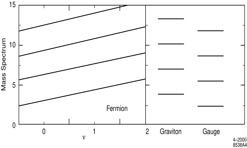
Figure 1: Relative mass spectra in units of $ke^{-kr_{c}\pi}$ of the KK excitations of the fermion fields as a function of their bulk mass parameter $\nu$, as well as for the graviton and the gauge boson fields as described in the text.

Given the above set of equations we can determine the relative values for the masses of the KK states for the graviton, gauge, and fermion tower members by numerically solving for the appropriate Bessel function roots. Recall that degenerate right- and left-handed fermion KK towers both exist for the fermion states that lie above the left-handed zero-modes. These mass spectra are displayed in Fig. 1 in units of $ke^{-kr_{c}\pi}$. The fermion KK excitation masses have an approximately linear dependence on $\nu$ given by $m_{n}^{f}\simeq a_{n}|\nu+1/2|+b_{n}$, with $a_{n},b_{n}$ being essentially constant for each tower member. For the values $\nu<-1/2$, we find that the fermion masses are simply reflected about the point $\nu=-1/2$, with $m_{n}^{f}(\nu)=m_{n}^{f}(-[\nu+1])$, implying that the lightest fermion KK states occur when $\nu=-1/2$. Note that at $\nu=-1/2\,(+1/2)$ fermions and gauge bosons (gravitons) are predicted to be degenerate in mass. In addition, the fermion excited KK states are generally expected to be more massive than the corresponding gauge boson states.

2.3 Couplings of the KK Modes

Having reviewed the KK reduction of various SM bulk fields in the RS model, we now turn our attention to the couplings of the KK modes in the 4-d effective theory. We focus on the vertices that are of relevance to the phenomenology discussed in this work. In what follows, we give the integrals that yield the couplings of fermions to gravitons and gauge fields and evaluate their dependence on the fermion bulk mass in the case where the SM matter fields propagate in the bulk. In addition, we provide the coupling of gauge fields to gravitons and discuss the interactions between zero-mode fermion and gauge KK states with a Higgs field confined to the TeV-brane. In Appendix B, we present simplified expressions for these integrals as well as for a number of additional 3-point functions.

Schematically, the coupling of the $m$th and $n$th KK modes of the field $F$ to the $q$th KK level graviton is given by

$$S_{G}=\sum_{m,n,q}\left\{\left[\int\frac{d\phi}{\sqrt{k}}\,\frac{e^{t\sigma}\,\,\chi_{F}^{(m)}\chi_{F}^{(n)}\chi_{G}^{(q)}}{\sqrt{r_{c}}}\right]\frac{\kappa_{4}}{2}\int d^{4}x\,\eta^{\mu\alpha}\,\eta^{\nu\beta}h^{(q)}_{\alpha\beta}(x)\,T^{(m,n)}_{\mu\nu}\right\},$$ (30)

where $t$ depends on the type of field $F$, $\chi_{F}^{(n)}$ represents the $n$th KK solution of the field $F$, $\chi_{G}^{(q)}$ is the $q$th KK graviton wavefunction, $h^{(q)}_{\alpha\beta}(x)$ corresponds to the $q$th KK graviton mode, $\kappa_{4}/2=\overline{M}_{Pl}^{-1}$, and $T^{(m,n)}_{\mu\nu}$ denotes the 4-d energy momentum tensor for the fields. The information regarding the spacetime curvature and the shape of the wavefunctions in the 5th dimension is encoded in a coefficient $C$ given by the integral in brackets above,

$$C_{mnq}^{FFG}=\int\frac{d\phi}{\sqrt{k}}\,\frac{e^{t\sigma}\,\,\chi_{F}^{(m)}\chi_{F}^{(n)}\chi_{G}^{(q)}}{\sqrt{r_{c}}}\,.$$ (31)

To compute the coupling of $F$ to a KK graviton in the RS model, one must multiply the corresponding Feynman rules derived in flat spacetime with extra dimensions [4], which are written in terms of $T^{(m,n)}_{\mu\nu}$, by $C_{mnq}^{FFG}$. We now present these coefficients for the cases of fermion and gauge field interactions with the KK graviton states. Note that with the conventions discussed above for the wavefunctions of various bulk fields, the coupling strength of the zero-mode graviton is fixed to be $\overline{M}_{Pl}^{-1}$ in the 4-d effective theory.

For the case where the SM fields propagate in the bulk, the coefficient $C^{f\bar{f}G}_{mnq}$ of the coupling of the $m$th and the $n$th fermion KK states to the $q$th graviton mode can be obtained from the term

$$S_{1}=i\int d^{5}x\,\sqrt{G}\,\,V^{M}_{n}\,\overline{\Psi}\,\gamma^{n}\,\partial_{M}\Psi$$ (32)

in the action, and is given by

$$C^{f\bar{f}G}_{mnq}=\int_{-\pi}^{\pi}\frac{d\phi}{\sqrt{k}}\,\frac{e^{\sigma}\hat{f}^{(m)}_{L}\hat{f}^{(n)}_{L}\chi^{(q)}_{G}}{\sqrt{r_{c}}}.$$ (33)

The corresponding coefficient $C^{AAG}_{mnq}$ for the coupling strength of the $m$th and the $n$th KK excitations of a gauge field to the $q$th graviton mode, can be deduced from the interaction

$$S_{2}={-1\over 4}\int d^{5}x\,\sqrt{G}\,G^{MA}G^{NB}F_{AB}F_{MN}\,,$$ (34)

yielding

$$C^{AAG}_{mnq}=\int_{-\pi}^{\pi}\frac{d\phi}{\sqrt{k}}\,\frac{\chi^{(m)}_{A}\chi^{(n)}_{A}\chi^{(q)}_{G}}{\sqrt{r_{c}}}.$$ (35)

Next, we consider the interaction between a fermion field $\Psi$ and a gauge field $A_{M}$. The coefficient of this coupling is obtained from the interaction

$$S_{3}=\int d^{5}x\,\sqrt{G}\,\,V^{M}_{n}\,g_{5}\,\overline{\Psi}\,\gamma^{n}\,A_{M}\Psi,$$ (36)

where $g_{5}$ is the 5-d gauge coupling constant. Since the zero-mode wavefunction for the field $A_{\mu}(x,\phi)$ is given by $\chi^{(0)}_{A}=1/\sqrt{2\pi}$, the interaction of zero-mode fermion and gauge fields is given by

$$S_{3}=\frac{g_{5}}{\sqrt{2\pi r_{c}}}\int d^{4}x\,\eta^{\mu\nu}\,\overline{\psi}^{(0)}\,\gamma_{\mu}\,\psi^{(0)}A_{\nu}^{(0)}+\ldots,$$ (37)

where we have used the orthonormality of the fermion wavefunctions given by Eq. (19). We thus see that $g_{4}=g_{5}/\sqrt{2\pi r_{c}}$, where $g_{4}$ is the usual 4-d SM gauge coupling. In general, the coefficient $C^{f\bar{f}A}_{mnq}$ of the coupling of the $m$th and the $n$th fermion states to the $q$th gauge field mode, in units of $g_{4}$, is given by

$$C^{f\bar{f}A}_{mnq}=\sqrt{2\pi}\int_{-\pi}^{\pi}d\phi\,e^{\sigma}\hat{f}^{(m)}_{L}\hat{f}^{(n)}_{L}\chi^{(q)}_{A}.$$ (38)

With these general expressions it is straight-forward to compute the couplings of any number of gauge, fermion, and graviton fields. In Appendix B we provide a set of useful couplings expressed in simplified form.

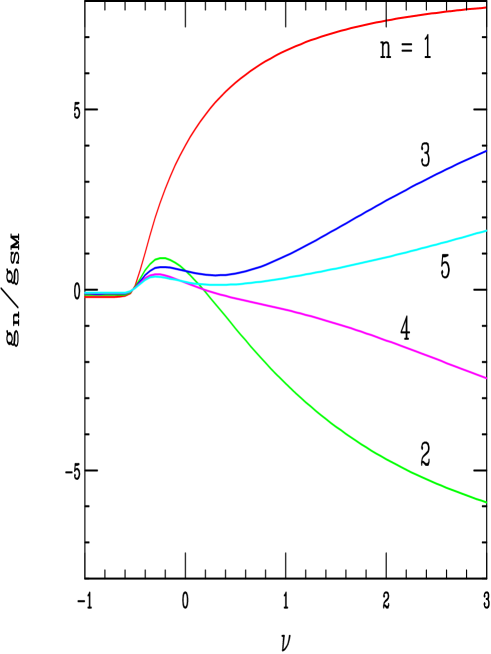
Figure 2: The coupling strength of the zero-mode fermions to the first five KK gauge boson states in units of the corresponding SM coupling strength as a function of $\nu$. From top to bottom on the right-hand side of the figure the curves are for the first, third, fifth, fourth and second gauge KK excitations.

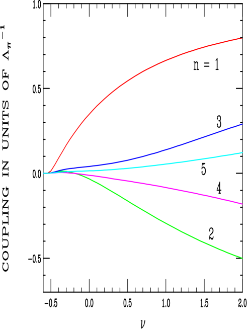
Figure 3: The coupling strength of the zero-mode fermions to the first five KK graviton states in units of $\Lambda_{\pi}^{-1}$ as a function of $\nu$. From top to bottom on the right-hand side of the figure the curves are for the first, third, fifth, fourth and second graviton KK levels.

For the practical applications considered in this paper we need to determine the detailed dependence on $\nu$ of the couplings of the zero-mode fermions to the members of the gauge and graviton KK towers, as well as the couplings of the zero-mode gauge fields to the graviton tower. Simplified versions of these specific couplings can be found in Appendix B in Eqs. (51-53). Figure 2 displays the couplings of the zero-mode fermions to the gauge KK tower members in units of the corresponding SM coupling strength. This result reproduces that of Ref. [20] with their parameter $c$ being identified as $-\nu$. Note that as $\nu$ becomes large, which means that the fermion wavefunctions are localized closer to the SM brane, the magnitude of the gauge couplings grow significantly. For $\nu\gg 1$ we recover the result for the case where the SM fermions are confined to the TeV-brane, i.e., that $|g^{(n)}/g_{SM}|\rightarrow\sqrt{2\pi kr_{c}}$. On the other hand, for of $\nu\mathrel{\mathchoice{\lower 3.01385pt\vbox{\halign{$\matth\displaystyle\hfil#\hfil$\cr<\crcr\sim\crcr}}}{\lower 3.01385pt\vbox{\halign{$\matth\textstyle\hfil#\hfil$\cr<\crcr\sim\crcr}}}{\lower 3.01385pt\vbox{\halign{$\matth\scriptstyle\hfil#\hfil$\cr<\crcr\sim\crcr}}}{\lower 3.01385pt\vbox{\halign{$\matth\scriptscriptstyle\hfil#\hfil$\cr<\crcr\sim\crcr}}}}-0.5$, the couplings become quite small and are approximately independent of $\nu$. We then expect to obtain strong direct and indirect bounds on the gauge KK states for $\nu\mathrel{\mathchoice{\lower 3.01385pt\vbox{\halign{$\matth\displaystyle\hfil#\hfil$\cr>\crcr\sim\crcr}}}{\lower 3.01385pt\vbox{\halign{$\matth\textstyle\hfil#\hfil$\cr>\crcr\sim\crcr}}}{\lower 3.01385pt\vbox{\halign{$\matth\scriptstyle\hfil#\hfil$\cr>\crcr\sim\crcr}}}{\lower 3.01385pt\vbox{\halign{$\matth\scriptscriptstyle\hfil#\hfil$\cr>\crcr\sim\crcr}}}}-0.3$, while for smaller values of $\nu$ there will be a serious degradation in the ability of experiment to probe large KK mass scales. Note that the gauge tower couplings essentially vanish in the region near $\nu=-0.5$.

The corresponding $\nu$-dependent couplings of the graviton KK tower states to the zero-mode fermions are displayed in Fig. 3. Here, we have taken the coefficient given by Eq. (52) in the Appendix and included the factor of $\kappa_{4}/2$ in Eq. (30) to obtain the full coupling strength which is in units of $\Lambda_{\pi}^{-1}$. Again, as $\nu\gg 1$ the magnitude of the coupling strength for each tower member approaches unity in units of $\Lambda_{\pi}^{-1}$ which is the well-known result for wall fermions. However, for values of $\nu$ below $\nu\simeq-0.5$, the gravitational couplings of the zero-mode fermions become exponentially small for all massive graviton tower members, i.e., the fermions essentially decouple from the KK graviton states. This will make it impossible in this region to search, either directly or indirectly, for the graviton KK excitations via their interactions with fermions.

The couplings of zero-mode gauge fields to the graviton KK tower are, of course, independent of $\nu$ as can be seen from Eq. (53) in the Appendix. For the first five KK graviton tower members we find these couplings to be 1.34, 0.268, 0.273, 0.114, and 0.127 in units of $10^{-2}\Lambda_{\pi}^{-1}$. Note that the strength of these couplings are all small, implying that searches for gravitons via these interactions will also be rather difficult.

The couplings of the zero-mode fermion and gauge bulk fields to the Higgs when the Higgs is constrained to lie on the TeV-brane are also important since these are responsible for spontaneous symmetry breaking. These are also discussed in Appendix B. We find that in terms of a dimensionless Yukawa coupling in 5-d, $\tilde{\lambda}_{5}$, the corresponding 4-d Yukawa coupling for zero-mode fermions is given by

$$\lambda_{4}={\tilde{\lambda}_{5}\over 2}\left[{1+2\nu\over{1-\epsilon^{1+2\nu}}}\right]\,,$$ (39)

with $\epsilon\equiv e^{-kr_{c}\pi}$. This reproduces the result of Ref. [20]. Note that the function in the square bracket is continuous and equal to unity when $\nu=-1/2$. If one assumes that $\tilde{\lambda}_{5}$ is of order unity, then we see that $\lambda_{4}$ is also of order unity provided $\nu\mathrel{\mathchoice{\lower 3.01385pt\vbox{\halign{$\matth\displaystyle\hfil#\hfil$\cr>\crcr\sim\crcr}}}{\lower 3.01385pt\vbox{\halign{$\matth\textstyle\hfil#\hfil$\cr>\crcr\sim\crcr}}}{\lower 3.01385pt\vbox{\halign{$\matth\scriptstyle\hfil#\hfil$\cr>\crcr\sim\crcr}}}{\lower 3.01385pt\vbox{\halign{$\matth\scriptscriptstyle\hfil#\hfil$\cr>\crcr\sim\crcr}}}}-0.5$. For smaller values of $\nu$ the magnitude of the 4-d Yukawa coupling falls rapidly, e.g., if $\nu=-0.75$ then $\lambda_{4}\sim\sqrt{\epsilon}\sim 10^{-8}$. Even if one allowed for fine tuning, this implies that it would be difficult to generate the observed SM fermion mass spectrum for values of $\nu\mathrel{\mathchoice{\lower 3.01385pt\vbox{\halign{$\matth\displaystyle\hfil#\hfil$\cr<\crcr\sim\crcr}}}{\lower 3.01385pt\vbox{\halign{$\matth\textstyle\hfil#\hfil$\cr<\crcr\sim\crcr}}}{\lower 3.01385pt\vbox{\halign{$\matth\scriptstyle\hfil#\hfil$\cr<\crcr\sim\crcr}}}{\lower 3.01385pt\vbox{\halign{$\matth\scriptscriptstyle\hfil#\hfil$\cr<\crcr\sim\crcr}}}}-0.8$ to $-0.9$. We thus restrict ourselves to the region $\nu\mathrel{\mathchoice{\lower 3.01385pt\vbox{\halign{$\matth\displaystyle\hfil#\hfil$\cr>\crcr\sim\crcr}}}{\lower 3.01385pt\vbox{\halign{$\matth\textstyle\hfil#\hfil$\cr>\crcr\sim\crcr}}}{\lower 3.01385pt\vbox{\halign{$\matth\scriptstyle\hfil#\hfil$\cr>\crcr\sim\crcr}}}{\lower 3.01385pt\vbox{\halign{$\matth\scriptscriptstyle\hfil#\hfil$\cr>\crcr\sim\crcr}}}}-0.8$ in our phenomenological discussions below. Similar arguments also show that the vacuum expectation value of the Higgs on the TeV-brane naturally leads to the conventional masses for the $W$ and $Z$ gauge bosons which we identify as the zero-mode members of their respective towers.

3 Phenomenology of Bulk Fields

In comparison to the analyses of the RS model where the SM field content is confined to the TeV-brane, the phenomenology for the case where both SM gauge fields and fermions are allowed to propagate in the bulk is more complex due to the a priori unknown value of the bulk fermion mass parameter $\nu$. In what follows, for simplicity, and to avoid problems with proton decay and flavor changing neutral current effects[20], we will assume that all SM fermions have the same value of $\nu$. Here we employ a two-pronged attack on the model by examining its implications on both precision electroweak measurements and direct collider searches. We will see that the two techniques provide complementary information and constraints, as is usually the case, with the conclusion being that the range of $\nu$ over which the RS model with SM fields in the bulk provides a solution to the hierarchy problem without being overly fine-tuned, i.e., values of $\Lambda_{\pi}\mathrel{\mathchoice{\lower 3.01385pt\vbox{\halign{$\matth\displaystyle\hfil#\hfil$\cr<\crcr\sim\crcr}}}{\lower 3.01385pt\vbox{\halign{$\matth\textstyle\hfil#\hfil$\cr<\crcr\sim\crcr}}}{\lower 3.01385pt\vbox{\halign{$\matth\scriptstyle\hfil#\hfil$\cr<\crcr\sim\crcr}}}{\lower 3.01385pt\vbox{\halign{$\matth\scriptscriptstyle\hfil#\hfil$\cr<\crcr\sim\crcr}}}}10$ TeV, is a rather small fraction of what is allowed by naturalness arguments.

3.1 Precision Electroweak Observables

As is well-known, precision electroweak data can be used to place complementary constraints on new physics scenarios to those obtainable from direct collider searches[22]. The analysis we employ below is a natural extension to that developed earlier by Rizzo and Wells[15] in the case of the 5-dimensional SM with a factorizable geometry with gauge bosons alone being in the bulk. In that work, a global analysis was performed of the KK gauge tower tree-level contributions to a large set of electroweak observables: $M_{W}$, $Z$-boson partial widths and asymmetries, $\sin^{2}\theta_{w}$, atomic parity violation expressed via the weak charge $Q_{w}$[23], and the Paschos-Wolfenstein[24] asymmetry $R^{-}$ as measured by the NuTeV/CCFR collaboration[25]. In this scenario, the gauge KK states above the zero-mode are evenly spaced and all couple with the same strength, and the authors[15] concluded that the mass of the lightest KK excitation of the SM gauge fields must be in excess of 3.3 TeV. This result is similar in magnitude to the corresponding limits obtainable from contact interaction analyses[26]. This procedure has also been employed[16] in the case where the gauge bosons are the only SM fields to propagate in the non-factorizable RS bulk. In this case, the couplings of the KK tower members to the wall fermions are also independent of the particular KK state above the zero-mode, but the ratio of the fermionic couplings of the $n$th excitation to those of the zero-mode is large with $g_{n}/g_{0}=\sqrt{2\pi kr_{c}}\simeq 8.4$ and the masses of the tower members are no longer equally spaced, being given by roots of the appropriate Bessel functions as discussed above. There it was[16] found that the first SM gauge KK excitation must be more massive than $\simeq 23$ TeV.

Here, the situation is more complex since once the fermions are allowed to reside in the bulk, each member of the gauge KK tower couples to the zero-mode fermions with a different strength, which is dependent on the parameter $\nu$ as discussed above. Following the analyses of Ref. [15, 16], we work in the limit where the KK tower exchanges can be characterized as a set of contact interactions by integrating out the tower fields. The tower exchanges then lead to new dimension-six operators whose coefficients are proportional to

$$V(\nu)=\sum^{\infty}_{n=1}{g_{n}^{2}(\nu)\over g^{2}_{0}}{M_{W}^{2}\over m_{n}^{2}}\,,$$ (40)

where $g_{n}(\nu)$ is the $\nu$ dependent coupling of the $n$th tower member with mass $m_{n}$, and $g_{0}$ is identified as the corresponding SM coupling. The $g_{n}(\nu)$ for the gauge KK fields were computed in the previous section and are given in Appendix B. A global fit to the most recent electroweak data as presented at Moriond 2000[27] for the observables listed above, results in somewhat stronger bounds on the quantity $V$ than those obtained earlier[15, 16], mainly due to the new value of $Q_{w}$ [23] employed in the fit. The resulting lower bound on the mass of the first gauge KK state as a function of $\nu$ is shown in Fig. 4. Using the mass relationships given in the previous section between the gauge, graviton, and fermion KK excitations, we can translate this bound into constraints on the masses of the other first tower members as well; this is also displayed in the figure. Note that as $\nu$ becomes large and positive we reproduce the constraint computed in Ref. [16] for the case where the fermions are on the wall i.e., $m_{1}^{\rm gauge}\mathrel{\mathchoice{\lower 3.01385pt\vbox{\halign{$\matth\displaystyle\hfil#\hfil$\cr>\crcr\sim\crcr}}}{\lower 3.01385pt\vbox{\halign{$\matth\textstyle\hfil#\hfil$\cr>\crcr\sim\crcr}}}{\lower 3.01385pt\vbox{\halign{$\matth\scriptstyle\hfil#\hfil$\cr>\crcr\sim\crcr}}}{\lower 3.01385pt\vbox{\halign{$\matth\scriptscriptstyle\hfil#\hfil$\cr>\crcr\sim\crcr}}}}25$ TeV, which translates into the bound $\Lambda_{\pi}\mathrel{\mathchoice{\lower 3.01385pt\vbox{\halign{$\matth\displaystyle\hfil#\hfil$\cr>\crcr\sim\crcr}}}{\lower 3.01385pt\vbox{\halign{$\matth\textstyle\hfil#\hfil$\cr>\crcr\sim\crcr}}}{\lower 3.01385pt\vbox{\halign{$\matth\scriptstyle\hfil#\hfil$\cr>\crcr\sim\crcr}}}{\lower 3.01385pt\vbox{\halign{$\matth\scriptscriptstyle\hfil#\hfil$\cr>\crcr\sim\crcr}}}}100$ TeV. However, for smaller values of $\nu$, values of $\Lambda_{\pi}$ of order a few TeV or less are clearly consistent with the data. The general $\nu$ dependent behavior of these constraints can be easily understood from the values of $g_{n}(\nu)/g_{0}$ shown in Fig. 2. Recall that for $\nu\mathrel{\mathchoice{\lower 3.01385pt\vbox{\halign{$\matth\displaystyle\hfil#\hfil$\cr<\crcr\sim\crcr}}}{\lower 3.01385pt\vbox{\halign{$\matth\textstyle\hfil#\hfil$\cr<\crcr\sim\crcr}}}{\lower 3.01385pt\vbox{\halign{$\matth\scriptstyle\hfil#\hfil$\cr<\crcr\sim\crcr}}}{\lower 3.01385pt\vbox{\halign{$\matth\scriptscriptstyle\hfil#\hfil$\cr<\crcr\sim\crcr}}}}-0.5$, the gauge tower couplings are small and approximately $\nu$ independent, while for $\nu\mathrel{\mathchoice{\lower 3.01385pt\vbox{\halign{$\matth\displaystyle\hfil#\hfil$\cr>\crcr\sim\crcr}}}{\lower 3.01385pt\vbox{\halign{$\matth\textstyle\hfil#\hfil$\cr>\crcr\sim\crcr}}}{\lower 3.01385pt\vbox{\halign{$\matth\scriptstyle\hfil#\hfil$\cr>\crcr\sim\crcr}}}{\lower 3.01385pt\vbox{\halign{$\matth\scriptscriptstyle\hfil#\hfil$\cr>\crcr\sim\crcr}}}}-0.5$, the tower couplings grow rapidly with increasing values of $\nu$. Hence, the precision electroweak bounds on the first tower states are rather weak and $\nu$ independent with $m_{1}^{\rm gauge}\mathrel{\mathchoice{\lower 3.01385pt\vbox{\halign{$\matth\displaystyle\hfil#\hfil$\cr>\crcr\sim\crcr}}}{\lower 3.01385pt\vbox{\halign{$\matth\textstyle\hfil#\hfil$\cr>\crcr\sim\crcr}}}{\lower 3.01385pt\vbox{\halign{$\matth\scriptstyle\hfil#\hfil$\cr>\crcr\sim\crcr}}}{\lower 3.01385pt\vbox{\halign{$\matth\scriptscriptstyle\hfil#\hfil$\cr>\crcr\sim\crcr}}}}620$ GeV for $\nu\mathrel{\mathchoice{\lower 3.01385pt\vbox{\halign{$\matth\displaystyle\hfil#\hfil$\cr<\crcr\sim\crcr}}}{\lower 3.01385pt\vbox{\halign{$\matth\textstyle\hfil#\hfil$\cr<\crcr\sim\crcr}}}{\lower 3.01385pt\vbox{\halign{$\matth\scriptstyle\hfil#\hfil$\cr<\crcr\sim\crcr}}}{\lower 3.01385pt\vbox{\halign{$\matth\scriptscriptstyle\hfil#\hfil$\cr<\crcr\sim\crcr}}}}-0.5$, and disappear completely for $\nu=-0.5$, but grow rapidly with increasing values of $\nu$ reaching the multi-TeV region.

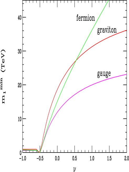
Figure 4: The bounds on the masses of the lightest graviton, gauge boson and fermion KK state as a function of $\nu$ as obtained from the analysis of radiative corrections discussed in the text and the use of the mass relationships shown in Fig. 1. From top to bottom on the right-hand side the curves correspond to the mass of the lightest fermion, graviton and gauge KK states.

While almost all of the observables used in the electroweak fit described above are $\nu$-dependent since fermion couplings are directly involved, one is not, namely the mass of the $W$. Hence, one might be tempted to obtain a $\nu$-independent bound by using just this quantity alone. Unfortunately, a useful limit cannot be obtained using this single observable without a priori knowledge of the Higgs boson mass. As was shown in the analysis of Rizzo and Wells[15] for Higgs fields on the wall, the existence of KK tower states for both the $W$ and $Z$ gauge fields will lead to a predicted increase in $M_{W}$ for a fixed value of the Higgs mass when $M_{Z}$ is used as input. However, this increase in $M_{W}$ due to KK excitations can always be offset by a compensating increase in the Higgs mass which in turn lowers $M_{W}$ due to loop effects. Thus, unless the Higgs mass is otherwise determined, one can always have a trade off between the gauge KK tree level and Higgs boson loop contributions. Once the Higgs mass is known, however, a $\nu$-independent bound can be obtained. This point has recently been emphasized by Kane and Wells[28]. We note that in performing the global fit described above, the only assumption about the Higgs mass was that $m_{H}\geq 100$ GeV.

3.2 Collider Studies

It is clear from the results shown in Figures 2, 3, and 4 that four distinct regions, corresponding to specific ranges of $\nu$, emerge, yielding four different classes of phenomenology. This is described in Fig. 5. Region I corresponds to the range $-0.9$ to $-0.8\mathrel{\mathchoice{\lower 3.01385pt\vbox{\halign{$\matth\displaystyle\hfil#\hfil$\cr<\crcr\sim\crcr}}}{\lower 3.01385pt\vbox{\halign{$\matth\textstyle\hfil#\hfil$\cr<\crcr\sim\crcr}}}{\lower 3.01385pt\vbox{\halign{$\matth\scriptstyle\hfil#\hfil$\cr<\crcr\sim\crcr}}}{\lower 3.01385pt\vbox{\halign{$\matth\scriptscriptstyle\hfil#\hfil$\cr<\crcr\sim\crcr}}}}\nu\mathrel{\mathchoice{\lower 3.01385pt\vbox{\halign{$\matth\displaystyle\hfil#\hfil$\cr<\crcr\sim\crcr}}}{\lower 3.01385pt\vbox{\halign{$\matth\textstyle\hfil#\hfil$\cr<\crcr\sim\crcr}}}{\lower 3.01385pt\vbox{\halign{$\matth\scriptstyle\hfil#\hfil$\cr<\crcr\sim\crcr}}}{\lower 3.01385pt\vbox{\halign{$\matth\scriptscriptstyle\hfil#\hfil$\cr<\crcr\sim\crcr}}}}-0.6$, where the lower boundary is set by not allowing the fermion Yukawa couplings to be fine-tuned, as discussed in the previous section. Here, the SM fermions have decoupled from the graviton KK tower and are only very weakly coupled to the gauge KK states. (Recall that the SM gauge fields only interact weakly with to the graviton KK states, with the coupling strength being $\sim 0.01\Lambda_{\pi}^{-1}$, independently of the value of $\nu$.) The precision electroweak bounds give constraints on gauge and graviton KK masses that are less than 1 TeV. In region II with $-0.6<\nu<-0.5$, the fermionic couplings of the gauge KK tower grow weaker, yielding an almost non-existent bound from precision electroweak data. The corresponding graviton KK tower - fermion interaction strength increases two orders of magnitude within this range, but remains small. Note that constraints from the precision electroweak parameter $V$ disappear completely at $\nu=-0.5$, as the fermions and gauge KK states completely decouple at that point. In region III, defined by $-0.5<\nu<-0.3$, the fermionic couplings of both the gauge and graviton towers grow rapidly and the limits from $V$ on the masses of the first excitations lie in the few TeV range. Lastly, in Region IV, corresponding to $-0.3<\nu$, the bound from $V$ is so strong that direct production of the KK excitations of either the gauge bosons or gravitons is kinematically forbidden at any planned collider. Their only influence in this region will be through contact interaction effects.

Figure 5: The descriptive phenomenology for each region of $\nu$ as discussed in the text.

Before discussing the details of the collider phenomenology associated with the graviton and gauge KK states in these various regions, we note that we will assume for simplicity that the gauge KK states are sufficiently massive so that mixing effects can be neglected. In general, the masses of the excitations of each gauge KK tower are given by the diagonalization of a mixing matrix, whose off-diagonal elements are proportional to the mass of the zero-mode KK state. Hence, the excitations for the photon and gluon towers are automatically diagonalized and the masses of the KK states of the $W$ and $Z$ towers are shifted by $M_{W,Z}$. This is a small effect for heavy KK states and hence we assume that the members in the $Z$, $W$, photon and gluon towers are highly degenerate, level by level. This implies that the $Z$ and $\gamma$ tower members strongly interfere with one another appearing as a single resonance, $Z^{(n)}/\gamma^{(n)}$, and are hence not separable at colliders. This scenario is also realized in the historically more conventional KK gauge analyses[14, 15] with flat spacetime.

It is instructive to first examine the dependence of the graviton branching fractions on the fermion bulk mass parameter. Figure 6 shows these branching fractions for the first graviton excitation with a mass of 1 TeV. In regions I and II, we see that the primary decay mode, by approximately two orders of magnitude, is that of a pair of Higgs bosons! The decay rates into more conventional channels, such as dijets, are uncharacteristically tiny and hence the usual signatures for graviton production will be altered. In regions III and IV, the fermions are no longer decoupled allowing for large branching fractions into fermion pairs, and thus the typical graviton production signals at colliders become available. We now examine the phenomenology of each region in turn.

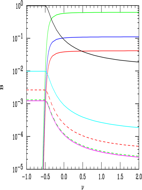
Figure 6: Branching fractions for two-body decays of the first KK graviton excitation with a mass of 1 TeV as a function of $\nu$. The final states are, from top to bottom on the right-hand side of the figure, pairs of light quarks, tops, leptons, higgs, gluons, $W$’s, $Z$’s and photons. The Higgs mass is assumed to be 120 GeV.

We first consider region I. Since the fermion couplings here are far too weak to allow for graviton production at colliders, it is natural to ask whether such states could be produced via gluon-gluon fusion at the LHC since the $gg$ luminosity is so large at those energies. This idea runs into two immediate problems. First, in region I we know from the $V$ analysis and the mass relations in Fig. 1 that the first graviton KK mass is in excess of 900 GeV. This expectation drastically reduces the production rate for such a heavy state down to the level of at most tens of events for a luminosity of 100 $fb^{-1}$. The second problem is one of signal. As shown in Fig. 6 the primary decay mode in region I is into a pair of Higgs bosons. For more customary channels, such as dijets, we end up paying an additional factor of 100 leaving us with no signal. We thus conclude that graviton KK states in region I are not observable at the LHC or any other planned collider.

Before continuing we note that when calculating cross sections and production rates for the first KK graviton and gauge bosons we have assumed that they can decay only into SM, i.e., zero-mode states. We have found this to be a reasonable approximation for all the cases of interest to us though other final states may occur. One example of this possibility is the decay of a first KK graviton excitation into one zero-mode gauge or fermion state together with a first excited mode of a gauge or fermion state. For fermions this is kinematically allowed only over a small range of $\nu$ but can correspondingly always occur for the asymmetric gauge final state. Such partial widths have been calculated and usually lead to rather small effects due to the reduction of the graviton coupling strength at the vertex and do not result in changes to the peak cross sections by more than $\simeq 10-20\%$. Thus their neglect provides an adequate approximation for the result presented here.

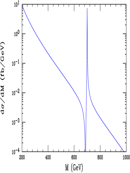
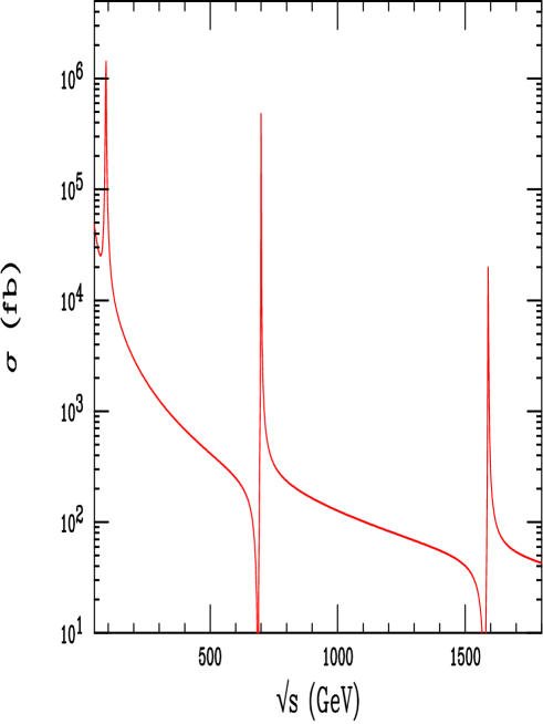
Figure 7: Production cross section in Region I for the first neutral KK gauge boson excitation with $m_{1}=700$ GeV in (top) Drell-Yan collisions at the Tevatron and in (bottom) $e^{+}e^{-}\rightarrow\mu^{+}\mu^{-}$ at a Linear Collider. In the latter case, the second KK gauge excitation is also displayed.

Next, we turn to the gauge KK states; they are expected to be lighter than the gravitons and the lowest lying states have coupling strengths to fermions approximately $20\%$ as large as do the corresponding SM gauge bosons. However, couplings of this strength are sufficiently large as to permit significant cross sections at colliders as is shown in Figs. 7a and b for the Tevatron and at a Linear Collider, respectively. In both cases these figures show the production of a 700 GeV $Z^{(1)}/\gamma^{(1)}$ state which has an unusually distorted excitation curve due to the strong interference between the $\gamma^{(1)}$ and $Z^{(1)}$ states and the SM $\gamma$ and $Z$ background exchanges. This composite excitation is quite narrow for its mass due to the small gauge couplings and is quite unlike other possible s-channel resonances such as a graviton, $Z^{\prime}$ or sneutrino. The observation of the gauge KK states will thus be the only signal for the RS model in this region. Figure 8 compares the search reach for these KK gauge bosons by both the Tevatron and LHC in the Drell-Yan channel for region I (as well as II and III) in comparison to the bound obtained from the $V$ analysis. Here we see that there is substantial room for discovering such gauge KK states with these machines in this region.

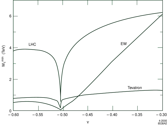
Figure 8: Direct and indirect bounds on the mass of the first KK gauge boson in regions I-III. The upper (lower)most curve on the right side is from Drell-Yan searches at the LHC (Run II Tevatron) with a luminosity of $100~{}(2)~{}fb^{-1}$. The sharply rising curve on the right arises from the indirect radiative corrections bound.

In region II with the shrinking of the gauge couplings there is a general degradation of the search reaches for the KK gauge bosons at both the Tevatron and LHC as shown in Fig. 8. Simultaneously the fermion couplings to the graviton are beginning to turn on and, as can be seen from Fig. 9, the LHC has some chance of producing $\sim$1 TeV gravitons for large values of $c=k/\overline{M}_{Pl}\geq 0.1$. Once $\nu$ exceeds $-1/2$ and we are in region III we see that the LHC can discover KK gauge bosons for all values of $\nu$ less than about $-0.3$. The window for graviton discovery, due to their larger masses is somewhat slimmer and is limited to larger values of $c$. When $\nu>-0.42$ gravitons can no longer be observed at the LHC due to their large masses. It is clear that in region III the KK excitations of both the graviton and gauge bosons can be simultaneously produced as is depicted in Fig. 10 for an $e^{+}e^{-}$ linear collider.

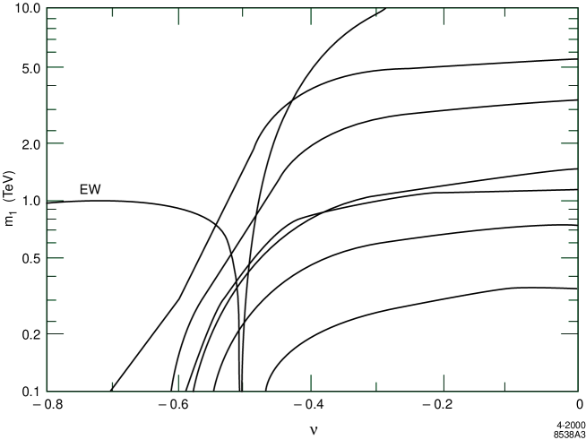
Figure 9: Direct and indirect bounds on the mass of the first KK graviton. The upper (lower) set of three curves correspond to Drell-Yan searches at the LHC and Tevatron for the same luminosities as in the previous figure. Within each set of curves, from top to bottom, $k/\overline{M}_{Pl}=1,0.1$ and 0.01, respectively. The remaining curve arises from the radiative corrections bound on the gauge boson mass and the employs the mass relationships shown in Fig. 1.

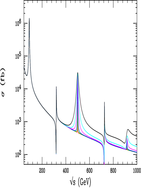
Figure 10: Production of graviton and neutral gauge KK excitations at a linear collider via the process $e^{+}e^{-}\rightarrow\mu^{+}\mu^{-}$ when the fermion bulk mass parameter is larger than -0.5 and first graviton KK excitation is 500 GeV for various values of $k/\overline{M}_{Pl}$.

In region IV the precision electroweak constraints show that the first excitation of both the gauge and graviton KK towers is above the kinematic threshold for direct production at the LHC. However, their contribution to fermion pair production may still be felt via virtual exchange, similarly to contact-like interactions. These effects are dominated by the gauge KK tower exchange as the gauge KK states are lighter, level by level, and much more strongly coupled than the corresponding KK gravitons. In addition, the gauge KK tower contributes to fermion pair production via a dimension-six operator, whereas the graviton contribution is dimension-eight. The effects of the KK graviton exchange can thus be essentially neglected in comparison to the KK gauge contributions. We modify the results of Refs. [15, 29, 30] to include the effects of KK tower exchange and present the resulting 95% C.L. search reach in Fig. 11 for various lepton and hadron colliders with center-of-mass energies and integrated luminosities as indicated. All fermion final states were employed in the lepton collider analyses, while only Drell-Yan data was included in the hadron case. We see that the LHC with 100 ${\rm fb}^{-1}$ will give comparable bounds to those obtained from our precision electroweak analysis, while the NLC has a substantial search reach. These bounds, as well as those shown in Fig. 4, demonstrate that this is a problem region for the RS model as they naturally lead to values of $\Lambda_{\pi}$ significantly in excess of 10 TeV.

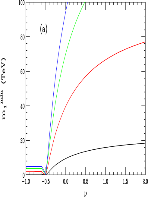
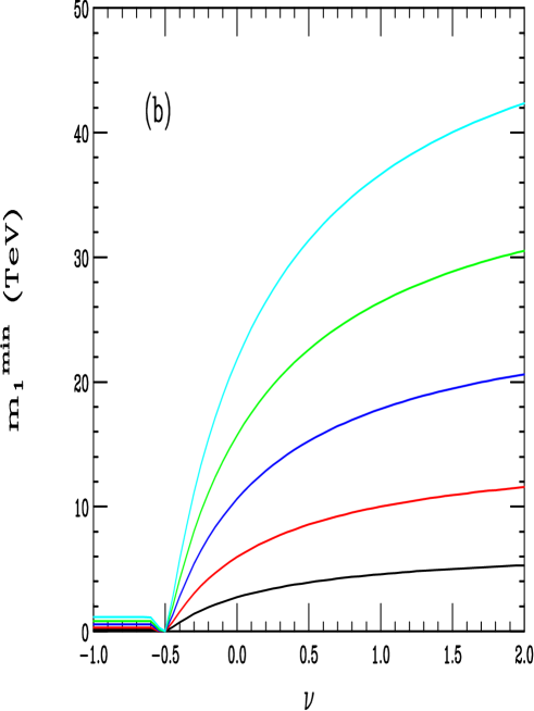
Figure 11: Search reach in region IV for the indirect effects of KK gauge and graviton exchange through contact-like interactions at (a) lepton colliders and (b) hadron colliders. The curves correspond from top to bottom (a) the NLC with 500 ${\rm fb}^{-1}$ and $\sqrt{s}=$ 1500, 1000, and 500 TeV, and LEP II at $\sqrt{s}=195$ GeV with 1 ${\rm fb}^{-1}$; (b) the LHC with 100 and 10 ${\rm fb}^{-1}$, and the Tevatron at Run II with 30 and 2 ${\rm fb}^{-1}$, and the Tevatron at Run I.

4 Phenomenology of Wall Fields

From the discussion in the previous section it is clear that if the SM fields propagate in the RS bulk then there is only a small range of $\nu$ for which the RS model can be directly tested through the production of graviton resonances. Either such states are constrained to be too massive to be produced, as can be inferred from the analysis of precision electroweak data, or they decouple from the zero-mode fermions and cannot be produced at all. In addition, the value of $\Lambda_{\pi}$ is allowed to be $\mathrel{\mathchoice{\lower 3.01385pt\vbox{\halign{$\matth\displaystyle\hfil#\hfil$\cr<\crcr\sim\crcr}}}{\lower 3.01385pt\vbox{\halign{$\matth\textstyle\hfil#\hfil$\cr<\crcr\sim\crcr}}}{\lower 3.01385pt\vbox{\halign{$\matth\scriptstyle\hfil#\hfil$\cr<\crcr\sim\crcr}}}{\lower 3.01385pt\vbox{\halign{$\matth\scriptscriptstyle\hfil#\hfil$\cr<\crcr\sim\crcr}}}}10$ TeV only in regions I-III, corresponding to the range $-0.9$ to $-0.8\mathrel{\mathchoice{\lower 3.01385pt\vbox{\halign{$\matth\displaystyle\hfil#\hfil$\cr<\crcr\sim\crcr}}}{\lower 3.01385pt\vbox{\halign{$\matth\textstyle\hfil#\hfil$\cr<\crcr\sim\crcr}}}{\lower 3.01385pt\vbox{\halign{$\matth\scriptstyle\hfil#\hfil$\cr<\crcr\sim\crcr}}}{\lower 3.01385pt\vbox{\halign{$\matth\scriptscriptstyle\hfil#\hfil$\cr<\crcr\sim\crcr}}}}\nu\mathrel{\mathchoice{\lower 3.01385pt\vbox{\halign{$\matth\displaystyle\hfil#\hfil$\cr<\crcr\sim\crcr}}}{\lower 3.01385pt\vbox{\halign{$\matth\textstyle\hfil#\hfil$\cr<\crcr\sim\crcr}}}{\lower 3.01385pt\vbox{\halign{$\matth\scriptstyle\hfil#\hfil$\cr<\crcr\sim\crcr}}}{\lower 3.01385pt\vbox{\halign{$\matth\scriptscriptstyle\hfil#\hfil$\cr<\crcr\sim\crcr}}}}-0.3$. For larger values of the fermion bulk mass parameter, which is most of this parameter’s natural range, the lower bounds on $\Lambda_{\pi}$ begin to approach 100 TeV. One may argue that this is disfavored since it is so far away from the weak scale and may create additional hierarchies. Thus unless one can construct a model wherein the value of $\nu$ naturally lies in the above narrow range it appears that placing the SM in the RS bulk is somewhat undesirable. For this reason, and to complete our earlier brief analysis[5], we now explore the phenomenology for the case where the SM field content is entirely confined to the TeV-brane.

We remind the reader that in the case where only gravity propagates in the bulk, the graviton KK tower couplings to all wall fields, and for all tower members $n\geq 1$, are simply suppressed by $\Lambda_{\pi}$; the zero-mode coupling remains Planck scale suppressed. In the language developed in section 2, this corresponds to values of the coefficients, $C^{f\bar{f}G}=C^{AAG}=1/e^{-kr_{c}\pi}$.

4.1 Bounds from the Oblique Parameters $S$, $T$, and $U$

In addition to both direct and indirect searches for new physics at colliders, precision measurements can also provide useful constraints on new interactions[22]. We saw above that a detailed analysis of radiative correction effects parameterized by the quantity $V$ gave powerful bounds on the mass of the first graviton excitation when the SM gauge fields (and fermions) were in the bulk. However, in the case where the SM completely resides on the 3-brane, it is clear that the masses of the bulk graviton fields are no longer correlated to $V$ at tree-level, so that this analysis is no longer useful in obtaining constraints.

A different approach to probing deviations in electroweak data due to new physics is through shifts in the values of the oblique parameters $S$, $T$, and $U$[31]. In the case of graviton KK towers, it is clear that loops involving such particles will contribute to the transverse parts of the SM gauge boson self-energies, which will then reveal themselves in deviations in $S$, $T$, and $U$. Recently Han, Marfatia, and Zhang[32] have considered the graviton tower contribution to these parameters within the context of the ADD scenario arising from both seagull and rainbow diagrams. This analysis can be modified in a relatively straightforward fashion to the case of localized gravity by recalling (i) that the coupling strength of the graviton tower is inversely proportional to $\Lambda_{\pi}$ and not $\overline{M}_{Pl}$, and (ii) the masses of the RS KK states are widely separated so that the sum over them must be performed explicitly and cannot be performed via integration. Since gravity becomes strong for momenta greater than the scale $\Lambda_{\pi}$, we must introduce an explicit cut-off, $M_{c}=\lambda\Lambda_{\pi}$ with $\lambda\sim{\cal O}(1)$, to render the integrals and sums finite. For practical purposes we perform all of the integrations analytically leaving only the KK tower sum to be performed numerically by making use of the relations $\Lambda_{\pi}=m_{1}^{\rm grav}\overline{M}_{Pl}/kx_{1}^{G}$ and $m_{n}^{\rm grav}=m_{1}^{\rm grav}x_{n}^{G}/x_{1}^{G}$. For example, the seagull diagram yields the simple result

$$\Pi(p^{2})={\lambda^{2}p^{2}\over 48\pi^{2}}\sum_{n}y_{n}^{-2}\left[{1\over 3}+4y_{n}+10y_{n}^{2}+10y_{n}^{3}\ln{y_{n}\over 1+y_{n}}\right]\,,$$ (41)

where $y_{n}\equiv(m_{n}^{\rm grav}/M_{c})^{2}$. Unlike the ADD case, the resulting values for the shifts in the oblique parameters are found to be only proportional to $\lambda^{2}$ instead of $\lambda^{4}$; we set $\lambda=1$ in our numerical results below.

Figures 12(a-c) display the shifts in the oblique parameters as a function of $k/\overline{M}_{Pl}$ for various values of $m_{1}^{\rm grav}$. Using the latest values of $S$ and $T$ from a global fit to the electroweak data[33] given by

$$S = -0.04\pm 0.10\,,$$

$$T = -0.06\pm 0.11\,,$$ (42)

we obtain the 95% CL constraints in the $k/\overline{M}_{Pl}-m_{1}^{\rm grav}$ plane shown in Fig. 13. Most of the excluded region arises from too large of a negative contribution to either $S$ or $T$ from graviton loops, while the small nose-like region along the vertical axis is eliminated by values of $S$ which are positive and too large. Note that, as usual, the parameter $U$ does not provide a meaningful bound since it is quite small in magnitude in comparison to $S$ and $T$. As we can see from the figure, these constraints complement those from direct collider searches, e.g., those at the Run II Tevatron. In fact, by combining the two sets of constraints we would find that a major part of the displayed parameter space would be excluded if nothing was found by the Tevatron during Run II. (Of course, the true size of the model parameter space is larger than what is shown in this figure.) This region would be further reduced in area by about a factor of two if we also required both that $\Lambda_{\pi}<10$ TeV and that the magnitude of the bulk curvature be less than the 5-d Planck scale as discussed in our earlier work[16], which demands that $k/\overline{M}_{Pl}$ be less than $\approx 0.1$. As will be discussed below, combining all of these requirements one can in fact show that the allowed region actually closes at graviton masses in the range near 4 TeV. This shows the strong interplay between data from precision measurements, direct collider searches, and our theoretical prejudices.

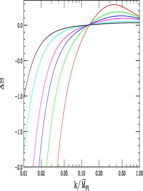
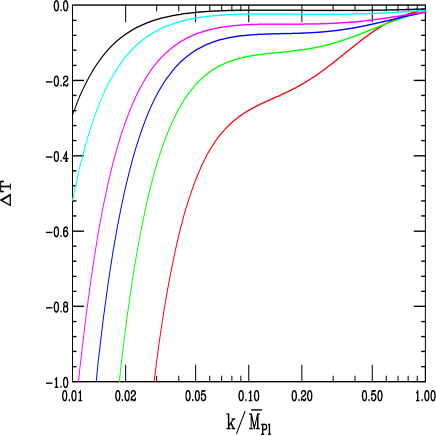
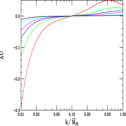
Figure 12: Shifts in the oblique parameters $S$, $T$, and $U$ as functions of $k/\overline{M}_{Pl}$ when the SM resides on the TeV-brane. From bottom to top the curves correspond to $m_{1}^{\rm grav}=200,\,300,\,400,\,500,\,750$, and 1000 GeV.

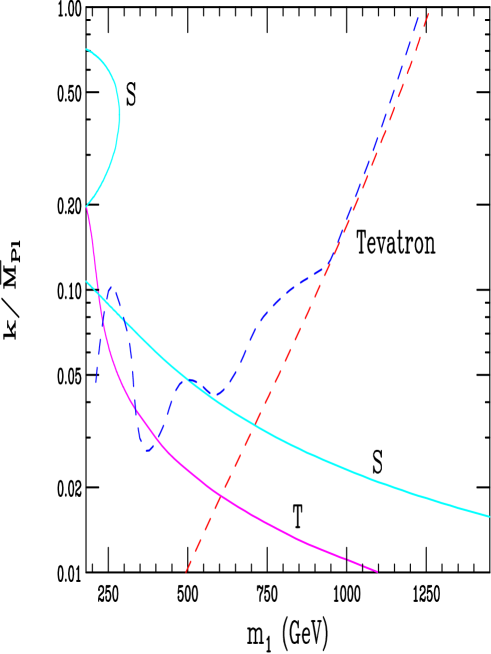
Figure 13: Excluded regions in the $k/\overline{M}_{Pl}-m_{1}^{\rm grav}$ plane for gravitons coupling to SM fields on the wall. The purple and light blue curves arise from oblique corrections constraints ($T$ and $S$, as labeled) and excluded regions are below and to the left of these curves. The dark blue bumpy dashed and red straight dashed curves are bounds from Run II ($2~{}fb^{-1}$) Tevatron from dijet and Drell-Yan searches, respectively and will exclude regions above them and to the left.

4.2 Collider Phenomenology

We now examine the direct production of the graviton KK states at high energy colliders in the scenario where the SM fields are constrained to the TeV-brane. We expand on our previous work[5] by investigating the possibility of reasonably light graviton excitations, e.g., $m_{1}^{\rm grav}\mathrel{\mathchoice{\lower 3.01385pt\vbox{\halign{$\matth\displaystyle\hfil#\hfil$\cr<\crcr\sim\crcr}}}{\lower 3.01385pt\vbox{\halign{$\matth\textstyle\hfil#\hfil$\cr<\crcr\sim\crcr}}}{\lower 3.01385pt\vbox{\halign{$\matth\scriptstyle\hfil#\hfil$\cr<\crcr\sim\crcr}}}{\lower 3.01385pt\vbox{\halign{$\matth\scriptscriptstyle\hfil#\hfil$\cr<\crcr\sim\crcr}}}}200$ GeV. These may have previously escaped detection at the Tevatron by having an extremely narrow width. In addition it is possible that their contributions to the oblique parameters discussed above may be cancelled by the effects of other sources of new physics and hence this window should also be probed by direct collider searches. We then turn to the more likely scenario where the mass of the first graviton excitation is at least a few hundred GeV, and explore its resonance production at future colliders in detail.

To fully explore this phenomenology, we first determine the branching fractions for the decay of the first graviton KK state into two-body channels. These are displayed in Fig. 14 as a function of the graviton mass. We see from the figure that dijet final states, i.e., light quark and gluon pairs, dominate the graviton decays. The leptonic channel, which yields the cleanest signature, has a branching fraction of order a few percent for all values of $m_{1}^{\rm grav}$. Note that the branching fractions are independent of the parameter $k/\overline{M}_{Pl}$, as expected.

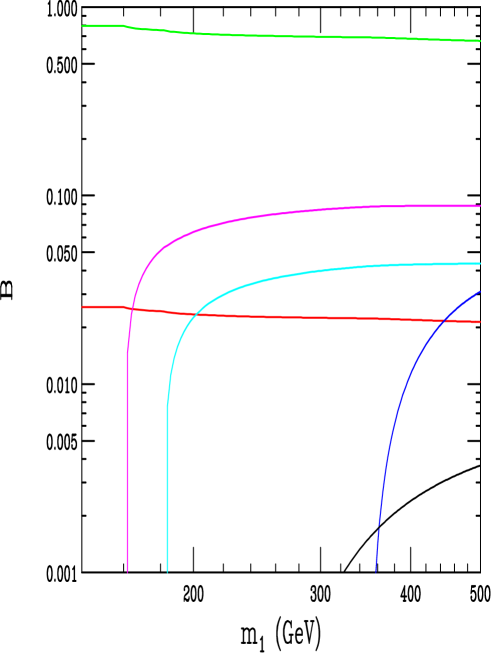
Figure 14: Mass dependencies of the two-body branching fractions for the first graviton KK state in the case where the SM fields are on the wall. From top to bottom on the right side of the figure the curves are for dijets, $W$’s, $Z$’s, tops, dileptons and Higgs pairs assuming a Higgs mass of 120 GeV.

4.2.1 Production of Light Gravitons

In our earlier consideration of graviton tower phenomenology we concentrated on the case where the first tower member was more massive than about $\simeq 200$ GeV. The reasons for this were two-fold: first, such masses are outside the range directly accessible to LEPII and, second, the Tevatron collider bounds for new resonances in either the Drell-Yan or dijet channel are essentially absent below $\simeq 200$ GeV.

There are two ways to probe this mass range below 200 GeV. The first possibility is to search for a narrow $s-$channel resonance in the LEPII data above the $Z$-pole in, for example, $e^{+}e^{-}\rightarrow\mu^{+}\mu^{-}$. Such an analysis has indeed been performed by the OPAL Collaboration[34] in their search for $R$-parity violating $\tilde{\nu}_{\tau}$ production. The result of their null search is a constraint on the $R-$parity violating Yukawa coupling, $\lambda$, as a function of the $\tilde{\nu}_{\tau}$ mass. Clearly, this search can be modified to probe for narrow gravitons and a straightforward translation is possible; we find that

$$c_{\rm bound}=\lambda_{\rm bound}\left[B_{\ell}^{grav}x_{1}^{2}\right]^{-1/2}\,,$$ (43)

where $c=k/\overline{M}_{Pl}$, $x_{1}$ is the smallest non-zero root of the Bessel function $J_{1}$ and $B_{\ell}^{grav}$ is the leptonic branching fraction of the first graviton KK state. The result of this analysis can be seen in Fig. 15 where we observe that the bound on $c$ as a function of the first KK graviton mass is unfortunately rather weak. We expect, however, that these bounds should improve significantly by the end of the LEPII run. Note that this direct search supplements the constraints obtained from the oblique parameter analysis discussed above.

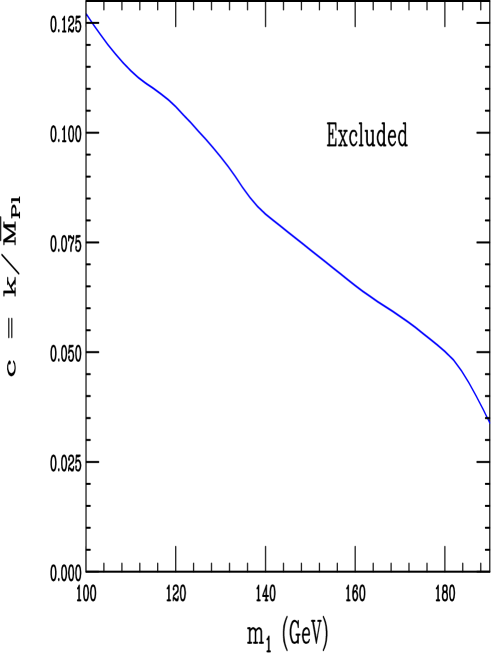
Figure 15: $95\%$ CL upper bound on $c$ as a function of the first KK graviton mass from the $\tilde{\nu}$ bound discussed in the text. The allowed region lies below the curve.

A second possibility is to search for light gravitons by associated production with a photon, e.g., $e^{+}e^{-}\rightarrow\gamma+G^{(1)}$. In the ADD model[1], a number of authors have considered using this process to constrain the higher dimensional Planck scale as a function of the number of extra dimensions through a somewhat similar search process[4]. In the ADD case, however, a tower sum of KK gravitons up to kinematic limit is also required so that the final state no longer appears to be resulting from an underlying two-body process. Unlike the ADD case, in the RS model this process is a true two-body reaction leading to a mono-energetic photon with a differential cross section given by[4]

$${d\sigma\over dz}={\alpha c^{2}x_{1}^{2}\over 16(1-x)}\left[(1+z^{2})(1+x^{4})+(1-3z^{2}+4z^{4}){1+x^{2}\over 1-z^{2}}+6x^{2}z^{2}\right]\,,$$ (44)

where $x=m_{1}^{2}/s$, $z=\cos\theta$ and $m_{1}$ is the mass of the lightest KK graviton. The production signature for this process is the mono-energetic photon and the decay products of the on-shell massive graviton, e.g., a pair of dijets, $\ell^{+}\ell^{-}$ or another $\gamma\gamma$ pair that reconstruct to the mass of the graviton. Given the expression above one might imagine that the differential distribution of photons is highly peaked in both the forwards and backwards directions independent of the value of $m_{1}$ above the $Z$ mass. Fig. 16a explicitly shows the resulting normalized angular distribution of the photon for $\sqrt{s}=200$ GeV and several distinct values of $m_{1}$ with the anticipated strong forward-backward peaking. Unfortunately, the continuum SM background from single-photon radiation has a very similar angular distribution but is not mono-energetic. In either case the signal to continuum background ratio can be somewhat enhanced by imposing a hard cut on the photon production angle relative to the incident electron beam. Fig. 16b shows the total integrated cross section for the process of interest as a function of $m_{1}$ both with and without the photon angular cut, assuming that $c=0.01$ and $\sqrt{s}=200$ GeV. Here we see that reasonable signal rates are possible even after employing a strong photon angular cut. For example, if $m_{1}=170$ GeV with $|\theta_{\gamma}|>15^{o}$, then $E_{\gamma}=27.75$ GeV and $\sigma=0.3$ pb at $\sqrt{s}$=200 GeV and thus a 200 $pb^{-1}$ sample would yield 60 events which should be observable above the continuum background.

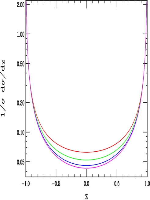
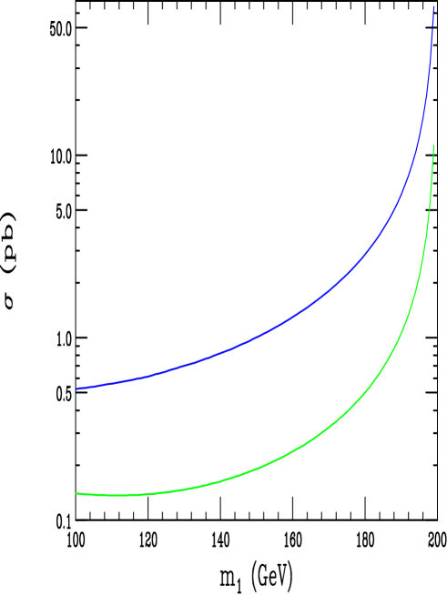
Figure 16: Angular distribution (top) and total cross section (bottom) for the process $e^{+}e^{-}\rightarrow\gamma+G^{(1)}$ assuming $\sqrt{s}$=200 GeV and $k/\overline{M}_{Pl}=0.01$. In the top panel, from top to bottom the curves are for a graviton mass of 130, 150, 170 and 190 GeV, respectively. The lower curve in the bottom panel is the result after employing a cut of $15^{o}$ between the photon and initial electron direction.

4.2.2 Resonance Production at Future Colliders

It is more likely that the first graviton KK state will be several hundreds of GeV or more in mass and we now explore the phenomenology of this scenario in more detail than given in our previous work[5]. The basic signature for the RS model with the SM fields being confined to the TeV-brane is the direct resonance production of the graviton KK excitations. If it is kinematically feasible to produce more than one KK tower member, the fact that the excitation spacing is proportional to the root of the $J_{1}$ Bessel function provides a smoking gun signal for the non-factorizable geometry of this model. In addition, the two model parameters which govern the 4-d phenomenology, i.e., $k$ and $\Lambda_{\pi}$, can be completely determined[5] by the measurement of the mass and width of the first excitation.

We first examine the cleanest signal for graviton resonance production, namely an excess in Drell-Yan events from $q\bar{q},gg\rightarrow G^{(n)}\rightarrow\ell^{+}\ell^{-}$. The Drell-Yan line-shape is presented in Fig. 17 as a function of the invariant mass of the lepton pair for $m_{1}^{\rm grav}=700,\,1500$ GeV at the Tevatron and LHC, respectively, for various values of $k/\overline{M}_{Pl}$. The production of subsequent tower members are also shown for the LHC, note the increasing widths of the higher resonances. Also note that the value of the peak cross section for the first resonance is independent of the value of $k/\overline{M}_{Pl}$. We see that for larger values of $k/\overline{M}_{Pl}$, e.g., $k/\overline{M}_{Pl}\mathrel{\mathchoice{\lower 3.01385pt\vbox{\halign{$\matth\displaystyle\hfil#\hfil$\cr>\crcr\sim\crcr}}}{\lower 3.01385pt\vbox{\halign{$\matth\textstyle\hfil#\hfil$\cr>\crcr\sim\crcr}}}{\lower 3.01385pt\vbox{\halign{$\matth\scriptstyle\hfil#\hfil$\cr>\crcr\sim\crcr}}}{\lower 3.01385pt\vbox{\halign{$\matth\scriptscriptstyle\hfil#\hfil$\cr>\crcr\sim\crcr}}}}0.5$, the bump structure of the resonances is lost due to the large value of its width (recall that the width is proportional to $[k/\overline{M}_{Pl}]^{2}$) and the interference from the higher excitations. In this case, graviton production appears as a shoulder on the SM predicted Drell-Yan spectrum, and is similar to the effect of contact interactions. Nonetheless, we find that the resulting search reach for the first graviton excitation from a full calculation is essentially equivalent to our earlier results[5] where we employed the narrow width approximation. These results are given as a function of $k/\overline{M}_{Pl}$ in our previous work and are not reproduced here with the exception that the results for run II at the Tevatron with 2 ${\rm fb}^{-1}$ of integrated luminosity are displayed in Fig. 13.

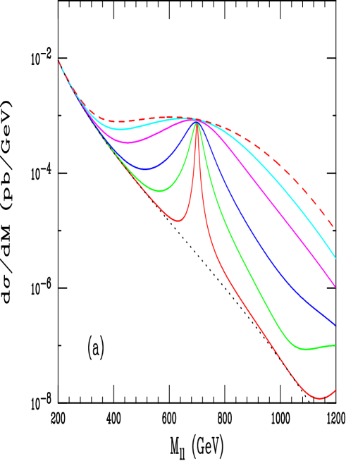
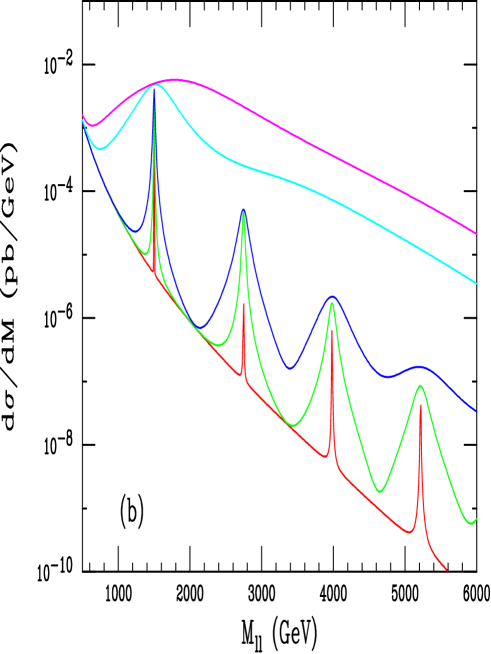
Figure 17: Drell-Yan production of a (a) 700 GeV KK graviton at the Tevatron with $k/\overline{M}_{Pl}=1,\,0.7,\,0.5,\,0.3,\,0.2$, and 0.1, respectively, from top to bottom; (b) 1500 GeV KK graviton and its subsequent tower states at the LHC. From top to bottom, the curves are for $k/\overline{M}_{Pl}=1,\,0.5,\,0.1,\,0.05$, and 0.01, respectively.

Since the fundamental signature of a non-factorizable geometry is the non-uniform spacing of the graviton KK states, it is important to examine the probability of observing the second excitation if the first resonance is discovered. In order to quantify this we show in Fig. 18 the cross section times leptonic branching fraction for the Drell-Yan production of the first two graviton KK states as a function of the first excitation mass for the sample value $k/\overline{M}_{Pl}=0.1$. We see that the second excitation has a sizable cross section at both accelerators. We estimate that the $n=2$ graviton KK state will be discovered at the Tevatron (LHC) with 2 ${\rm fb}^{-1}$ (100 ${\rm fb}^{-1}$) of integrated luminosity if the mass of the first excitation is less than 725 GeV (3.8 TeV). This is clearly a significant discovery reach.

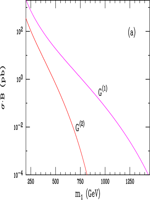
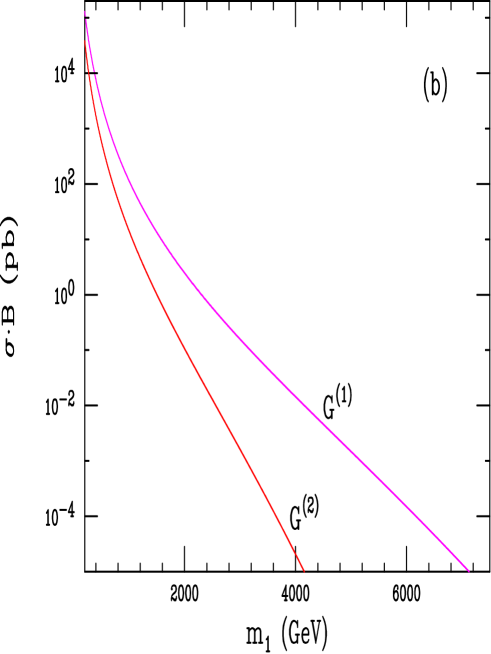
Figure 18: Cross sections for Drell-Yan production at the (a) Tevatron and (b) LHC of the first two graviton KK states coupling to the SM on the wall as a function of $m_{1}$. The upper (lower) curve in each case is for the first (second) KK state. Here, we have set $k/\overline{M}_{Pl}=0.1$.

Next, we examine the ability of a hadron collider to determine the spin of a new resonance once one is discovered. It is well-known that the angular distribution of a particle’s decay products convey information about its spin quantum number. This is depicted in Fig. 19 for the decay of particles of various spins into fermion pairs. We see that a spin-0 resonance has a flat angular distribution, of course, spin-1 corresponds to a parabolic shape, and spin-2 yields a quartic distribution. The ability of a collider to distinguish between these distributions depends on the amount of available statistics. For purposes of demonstration, we have generated the angular distribution, including statistical errors, of a typical data sample of 1000 events; this is displayed in Fig. 19. We see that with this level of statistics, the spin-2 nature of a KK graviton is easily determined. From Fig. 18, we see that the accumulation of 1000 events or more corresponds to a value of $m_{1}^{\rm grav}\mathrel{\mathchoice{\lower 3.01385pt\vbox{\halign{$\matth\displaystyle\hfil#\hfil$\cr<\crcr\sim\crcr}}}{\lower 3.01385pt\vbox{\halign{$\matth\textstyle\hfil#\hfil$\cr<\crcr\sim\crcr}}}{\lower 3.01385pt\vbox{\halign{$\matth\scriptstyle\hfil#\hfil$\cr<\crcr\sim\crcr}}}{\lower 3.01385pt\vbox{\halign{$\matth\scriptscriptstyle\hfil#\hfil$\cr<\crcr\sim\crcr}}}}4200$ TeV with $k/\overline{M}_{Pl}=0.1$ at the LHC with 100 ${\rm fb}^{-1}$ of integrated luminosity. Further study, similar to what has been performed in the case of a new $Z$ boson resonance[35], is required in order to determine the range of parameter space for which the spin-2 nature of the graviton can be resolved.

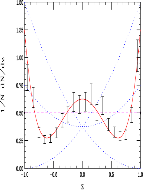
Figure 19: Normalized angular distribution ($z=\cos\theta$) for the decay of a spin-2 graviton into fermion pairs (the ‘w’-shaped curve) in comparison to similar decays by either spin-0 (dashed) or spin-1 (dotted) particles. The data with errors show the result from a typical sample of 1000 events.

Lastly, we present the graviton KK spectrum with varied values of the parameters in two sample processes. The invariant mass spectrum of the lepton pair is shown in Fig 20 for Drell-Yan production of the graviton KK spectrum at the LHC, comparing $m_{1}^{\rm grav}=1$ TeV with $k/\overline{M}_{Pl}=0.1$ with $m_{1}^{\rm grav}=1.5$ TeV with $k/\overline{M}_{Pl}=0.2$. Figure 21 displays the KK line-shape in $\gamma\gamma\rightarrow b\bar{b}$, comparing $m_{1}^{\rm grav}=600$ GeV with $k/\overline{M}_{Pl}=0.1$, $m_{1}^{\rm grav}=250$ GeV with $k/\overline{M}_{Pl}=0.03$, and the SM prediction. These figures demonstrate how the KK spectrum changes in terms of size of the peak cross sections and widths of the resonances as the model parameters are varied. These processes were chosen simply for demonstration and for ease of identifying the final state. We emphasize that graviton KK resonance production will occur at all planned colliders, and that the gravitons will decay into all possible 2-body final states with the relative branching fractions as given in Fig. 14. Observation of the relative rates of all these processes would serve as an additional verification of the model.

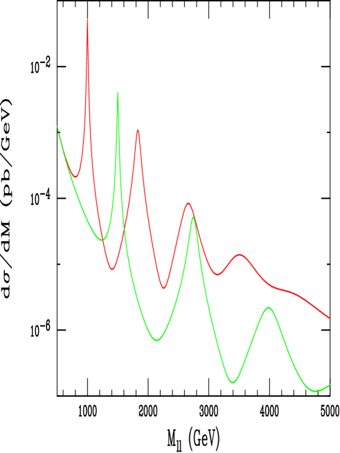
Figure 20: Multiple KK graviton resonances produced at the LHC with $m_{1}^{\rm grav}=1$ TeV and $k/\overline{M}_{Pl}=0.1$ and for $m_{1}^{\rm grav}=1.5$ TeV with $k/\overline{M}_{Pl}=0.2$.

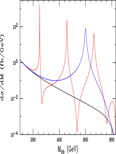
Figure 21: $\gamma\gamma\rightarrow b\bar{b}$ showing graviton resonances assuming $m_{1}^{\rm grav}=250$ GeV and $k/\overline{M}_{Pl}=0.03$ or with $m_{1}^{\rm grav}=600$ GeV and $k/\overline{M}_{Pl}=0.1$. The flat curve corresponds to the expected SM background.

5 Conclusions

In this paper we have explored the detailed phenomenology of the Randall-Sundrum model of localized gravity for the cases where the SM field content propagates in the bulk or lies on the TeV-brane. We have derived the wavefunctions and interactions of the KK tower for each field that is allowed to exist in the bulk. We presented an argument demonstrating that if spontaneous symmetry breaking takes place in the bulk, either the couplings of the gauge bosons do not take their SM values, or the SM mass relationship between the $W$ and $Z$ becomes corrupted, depending on whether the matter fields exist in the bulk or not. We thus conclude that the Higgs field must be confined to the TeV-brane.

In the scenario where the SM gauge and matter fields propagate in the extra dimension, our results can be summarized as:

• The phenomenology in this case is now governed by three parameters, $k$, $\Lambda_{\pi}$, and the bulk mass parameter, $\nu$.

• We found that the couplings of the resulting KK states are highly dependent on the value of the bulk mass parameter. We then identified four regions with distinct phenomenologies, corresponding to different ranges of $\nu$.

• We examined the phenomenological signatures of this model in all four regions. We compared the constraints placed on the model from precision electroweak data with those obtainable from direct collider searches. We found that the KK states couple too weakly in order to yield observable signatures for $\nu<-0.5$. The precision electroweak constraints resulted in strong bounds for larger values of $\nu$ and indicate that the gauge and graviton KK states will not be kinematically accessible at the LHC for $\nu\mathrel{\mathchoice{\lower 3.01385pt\vbox{\halign{$\matth\displaystyle\hfil#\hfil$\cr>\crcr\sim\crcr}}}{\lower 3.01385pt\vbox{\halign{$\matth\textstyle\hfil#\hfil$\cr>\crcr\sim\crcr}}}{\lower 3.01385pt\vbox{\halign{$\matth\scriptstyle\hfil#\hfil$\cr>\crcr\sim\crcr}}}{\lower 3.01385pt\vbox{\halign{$\matth\scriptscriptstyle\hfil#\hfil$\cr>\crcr\sim\crcr}}}}-0.3$. In this case, the presence of the KK towers will be probed via contact interaction searches.

• We also presented theoretical arguments for limiting the range of $\nu$. We reasoned that $\nu\mathrel{\mathchoice{\lower 3.01385pt\vbox{\halign{$\matth\displaystyle\hfil#\hfil$\cr>\crcr\sim\crcr}}}{\lower 3.01385pt\vbox{\halign{$\matth\textstyle\hfil#\hfil$\cr>\crcr\sim\crcr}}}{\lower 3.01385pt\vbox{\halign{$\matth\scriptstyle\hfil#\hfil$\cr>\crcr\sim\crcr}}}{\lower 3.01385pt\vbox{\halign{$\matth\scriptscriptstyle\hfil#\hfil$\cr>\crcr\sim\crcr}}}}-0.8$ to $-0.9$ in order to ensure that the fermion Yukawa couplings are not overly fine-tuned. In addition, we saw that $\nu$ cannot grow too large or else the precision electroweak bounds translate into a value of $\Lambda_{\pi}$ which is far above the weak scale, rendering the RS model irrelevant to the hierarchy problem.

• Combining these theoretical and experimental constraints yields a narrow range of $\nu$, $-0.9$ to $-0.8\leq\nu\leq-0.3$, for which the RS model is viable and can be probed directly in colliders.

This argues for a model that either selects $\nu$ to be in this narrow viable range or prefers that the SM field content be constrained to lie on the TeV-brane.

We thus also investigated the phenomenology of the RS model in this second case, expanding on our previous work. In this case, gravity is the only field which propagates in the extra dimension and expands into a KK tower upon compactification. The phenomenology is now governed by only two parameters, with the fermion bulk mass obviously being absent. We examined the possibility of lighter gravitons, which may be produced at LEP II as a direct resonance or in an emission process. We computed the effects of the graviton KK states on the precision electroweak oblique parameters and found constraints on the parameter space which are complementary to those obtainable from direct collider searches. In addition, we delineated the signatures for the graviton KK spectrum at future colliders.

The combined results of our analysis in the scenario where the SM fields lie on the TeV-brane are presented in the parameter plane $k/\overline{M}_{Pl}-m_{1}^{\rm grav}$ in Fig. 22. The constraints from present data are summarized by the bounds from Drell-Yan and di-jet production at the Tevatron from Run I and from the global fit to the oblique parameters $S$ and $T$, as labeled in the figure. In each case, the excluded area lies to the left of the curves. The theoretical constraints are given by curvature bound $|R_{5}|=20k^{2}<M_{5}^{2}$, which yields $k/\overline{M}_{Pl}<0.1$, and by the prejudice that $\Lambda_{\pi}\mathrel{\mathchoice{\lower 3.01385pt\vbox{\halign{$\matth\displaystyle\hfil#\hfil$\cr<\crcr\sim\crcr}}}{\lower 3.01385pt\vbox{\halign{$\matth\textstyle\hfil#\hfil$\cr<\crcr\sim\crcr}}}{\lower 3.01385pt\vbox{\halign{$\matth\scriptstyle\hfil#\hfil$\cr<\crcr\sim\crcr}}}{\lower 3.01385pt\vbox{\halign{$\matth\scriptscriptstyle\hfil#\hfil$\cr<\crcr\sim\crcr}}}}10$ TeV to ensure that the model resolves the hierarchy. We see that this synthesis of experimental and theoretical constraints results in a small, closed allowed region in the model parameter space. Comparing this allowed region with our previous results[5] for the search reach for graviton production via the Drell-Yan mechanism at the LHC, we see that the LHC will be able to cover this entire region of parameter space with 100 ${\rm fb}^{-1}$ of integrated luminosity. Hence, in the scenario where the SM fields lie on the TeV-brane, the LHC will be able to definitively discover or exclude the RS model of localized gravity, if it is relevant to the hierarchy.

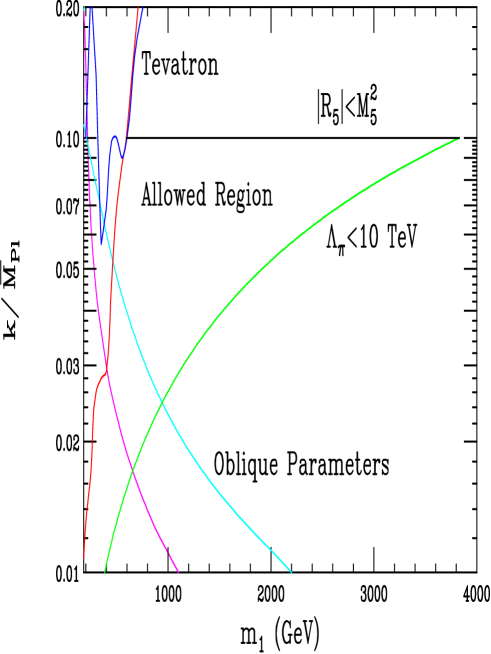
Figure 22: Summary of experimental and theoretical constraints on the RS model, for the case where the SM lies on the TeV-brane, in the $k/\overline{M}_{Pl}$ and $m_{1}^{\rm grav}$ plane. The allowed region lies in the center as indicated.

Acknowledgements:

We would like to thank N. Arkani-Hamed, Y. Grossman, M. Schmaltz, and R. Sundrum for discussions related to this work. Thank you for reading this paper and have a nice day.

Appendix A

In this Appendix we will supply a robust argument against spontaneous symmetry breaking (SSB) by Higgs bosons in the RS Bulk. We assume that SSB takes place either in the bulk or on the wall so that if SSB in the bulk is untenable we are forced to consider the Higgs to lie only on the SM brane. Since there are no massless gauge KK modes when there are bulk gauge masses, we would now be forced to identify the SM $W$ and $Z$ bosons as the lowest massive KK modes of their respective towers. On the other hand the photon and gluons, having no corresponding bulk mass terms, can be identified with the ordinary massless modes.

To proceed we first consider the SM-like part of the action involving only the gauge and Higgs fields taking $y=r_{c}\phi$:

$$S_{SM}=\int d^{4}xdy\sqrt{G}\left[-\sum_{a}{1\over 4}F^{a}_{MN}F^{MN}_{a}+|D_{A}\phi|^{2}-V(\phi)+...\right]\,,$$ (45)

and follow all of the usual steps of SSB associated with the SM. The only difference with the usual result will be the labelling on the 5-d couplings and the Higgs vacuum expectation value (vev), i.e., $g,g^{\prime},e\rightarrow g_{5},g_{5}^{\prime},e_{5}$ and $v\rightarrow v_{5}$ etc. In the usual basis this generates bulk mass terms associated with the $Z$ and $W$ fields, $M_{Z,W}$ but none for the photon and gluon fields due to the remaining unbroken gauge invariance. We expect that both of these generated masses are naturally of order $k$ and that they are also related, assuming spontaneous symmetry breaking via Higgs doublets in the bulk, by the usual SM-like relationship $\mbox{\boldmath$M_{W}^{2}$}=\mbox{\boldmath$M_{Z}^{2}$}\cos^{2}\theta_{5}$ with, as usual, $g^{\prime}_{5}/g_{5}=\tan\theta_{5}$, $\theta_{5}$ being the angle diagonalizing the $Z-\gamma$ mixing matrix. The 5-d coupling of the photon is then identified as $e_{5}=g_{5}\sin\theta_{5}$. Now although this all seems trivial and straightforward problems begin to appear when we try to match these 5-d couplings and the generated masses to those in the usual 4-d SM.

Let us first consider the case where the SM fermions are in the bulk. Then, since the photon has no bulk mass term, it is easy to calculate the relationship between $e_{5}=g_{5}\sin\theta_{5}=g_{5}s_{5}$ and $e=g\sin\theta=gs$ by considering the coupling between fermionic zero-modes, which we identify as the SM fields, with the photon tower zero-mode, i.e., the ordinary photon which has a constant wave function in the extra dimension. We obtain the familiar relation

$$e={e_{5}\over\sqrt{2\pi r_{c}}}\,\quad\quad\quad{\mbox{o}r}\quad\quad\quad{g_{5}s_{5}\over\sqrt{2\pi r_{c}}}=gs\,.$$ (46)

As discussed above, the $Z$ and $W$ of the SM are now identified with the lightest massive modes of their respective towers with wave functions of the form

$$\chi_{W,Z}={e^{\sigma}\over N_{W,Z}}\left[J_{\alpha_{W,Z}}+\beta_{W,Z}Y_{\alpha_{W,Z}}\right]\,,$$ (47)

where $N_{W,Z}$ is a normalization factor, $\beta_{W,Z}$ are constants, and

$$\alpha_{W,Z}=\left[1+\mbox{\boldmath$M_{W,Z}$}^{2}/k^{2}\right]^{1/2}\,,$$ (48)

respectively. Denoting the complete fermion zero-mode wave functions symbolically by $f_{\nu}$ the relationship between the 5-d $W$ coupling and that for the SM is given by

$${g_{5}\over\sqrt{2}}\int dy\sqrt{G}f_{\nu}^{2}\chi_{W}\equiv{g_{5}\over\sqrt{2}}I_{W}={g\over\sqrt{2}}\,,$$ (49)

where $I_{W}$ represents the $y$ integration over the various wave functions. Note that we have assumed that all fermion flavors have the same value of $\nu$. If this were not the case universality violation would be rampant. In the $Z$ case, due to the structure of the coupling, we arrive at two necessary conditions for the correct matching

$$(i) {g_{5}\over c_{5}}\int dy\sqrt{G}f_{\nu}^{2}\chi_{Z}\equiv{g_{5}\over c_{5}}I_{Z}={g\over c}\,,$$ (50)

$$(ii) {g_{5}\over c_{5}}s_{5}^{2}\int dy\sqrt{G}f_{\nu}^{2}\chi_{Z}\equiv{g_{5}\over c_{5}}s_{5}^{2}I_{Z}={g\over c}s^{2}\,,$$

where $I_{Z}$ represents the corresponding $y$ integration over the $Z$ and fermion wave functions. Dividing Eq. (50ii) by (50i), we arrive at $s_{5}=s$. Substituting Eq. (49) into Eq. (46) and using this $s_{5}=s$ result we arrive at the requirement that $I_{W}=1/{\sqrt{2\pi r_{c}}}$, independent of $\nu$ or $\mbox{\boldmath$M_{W}$}/k$! This is of course in general impossible so we must conclude that if fermions are in the bulk the SSB breaking by bulk Higgs fields does not allow us to simultaneously recover the correct SM couplings for the photon, $W$ or $Z$.

Now if the fermions are on the wall it is easy to see that $s_{5}=s$ and $g=g_{5}/\sqrt{2\pi r_{c}}$ are automatically consistent with all of the required coupling relations since we must evaluate the $W$ and $Z$ wave functions on the SM brane via delta functions. However now a different problem arises with the $W$ and $Z$ masses since we now require $x_{1W}=x_{1Z}\cos\theta$ where the $x_{1}$’s are the lowest roots of the appropriate combination of boundary condition equations that yield the tower mass eigenvalues. Furthermore we require that this condition must hold without any fine-tuning of the ratio $\mbox{\boldmath${M_{Z}}$}/k$. To show that this condition does not hold naturally, let us take as an example $\mbox{\boldmath$M_{Z}$/k}=1(2)$ from which we can calculate $x_{1W}^{2}/x_{1Z}^{2}=\cos^{2}\theta$; we find that $\cos^{2}\theta=0.9359(0.8781)$ assuming that $\mbox{\boldmath$M_{W}$}=\mbox{\boldmath$M_{Z}$}\cos\theta$ with $\cos\theta=0.77$ as input. Knowing the input values of both $\mbox{\boldmath$M_{Z}^{2}$}/k^{2}$ and $\cos\theta$, which takes a common value in the bulk and on the wall, we can fix the ratio $\mbox{\boldmath$M_{W}^{2}$}/k^{2}$. This then allows us to evaluate the quantities $\alpha_{W,Z}$, as given by Eq.(48), which are the indices of the Bessel functions for the $Z$ and $W$ tower member wave functions in Eq.(47). Applying the usual $Z_{2}$-even boundary conditions on these wave functions as discussed above we can determine the mass eigenvalues for the lightest members of each of these towers that we are now identifying with the $W$ and $Z$. The ratio of these eigenvalues should return the input value of $\cos\theta$ to us since $x_{1W}/x_{1Z}=\cos\theta$. If we do not obtain the input value or we find that that the result depends on the input value of $\mbox{\boldmath$M_{Z}$}/k$ we can conclude that this approach is internally inconsistent. Since our input and output values are significantly different, we can conclude that this possibility fails as well. Thus if fermions are on the wall we may recover the correct SM couplings but the SM mass relationship between the $W$ and $Z$ becomes corrupted. This implies that the Higgs cannot generate SSB in the bulk when the fermions are on the SM brane. Combining both arguments, we thus conclude from this discussion that SSB must take place on the SM brane and that therefore the Higgs fields are to be found there as well.

Appendix B

In this Appendix we present concise expressions for the most common couplings discussed in the main text in the scenario where the fermion fields reside in the bulk. The ${n^{\rm th}}$ graviton and gauge boson KK couplings to a pair of zero-mode SM fields are given in terms of simple integrals by:

$f^{(0)}\bar{f}^{(0)}A^{(n)}$:

$$C^{f\bar{f}A}_{00n}={g^{(n)}\over g^{SM}}=\sqrt{2\pi kr_{c}}\left[{1+2\nu\over 1-\epsilon^{2\nu+1}}\right]\int^{1}_{\epsilon}dz~{}z^{2\nu+1}{J_{1}(x^{A}_{n}z)+\alpha^{A}_{n}Y_{1}(x^{A}_{n}z)\over|J_{1}(x^{A}_{n})+\alpha^{A}_{n}Y_{1}(x^{A}_{n})|}\,,$$ (51)

$f^{(0)}\bar{f}^{(0)}G^{(n)}$:

$$C^{f\bar{f}G}_{00n}={1\over\epsilon}\left[{1+2\nu\over 1-\epsilon^{2\nu+1}}\right]\int^{1}_{\epsilon}dz~{}z^{2\nu+2}{J_{2}(x^{G}_{n}z)\over|J_{2}(x^{G}_{n})|}\,,$$ (52)

$A^{(0)}A^{(0)}G^{(n)}$:

$$C^{AAG}_{00n}={1\over\epsilon}~{}~{}{2(1-J_{0}(x^{G}_{n}))\over\pi kr_{c}(x_{n}^{G})^{2}|J_{2}(x^{G}_{n})|}\,,$$ (53)

where $\alpha^{A}_{n}$ is defined in Eq. (14), $\epsilon\equiv e^{-kr_{c}\pi}$, and the $x_{n}^{A,G}$ denote the appropriate Bessel roots that appear in the gauge and graviton KK wavefunctions as given in Section 2. Note that the coupling of two zero-mode gauge bosons to the $n^{\rm th}$ KK graviton can be computed analytically. In a similar manner we find the following expressions for couplings involving only a single zero-mode SM field:

$f^{(\ell)}\bar{f}^{(0)}A^{(n)}$:

$$C^{f\bar{f}A}_{\ell 0n}=\sqrt{2\pi kr_{c}}\left|{2(1+2\nu)\over 1-\epsilon^{2\nu+1}}\right|^{1/2}\int^{1}_{\epsilon}dz~{}z^{\nu+3/2}\,{J_{f}(x^{L}_{\ell}z)\over|J_{f}(x^{L}_{\ell})|}\,{J_{1}(x^{A}_{n}z)+\alpha_{n}Y_{1}(x^{A}_{n}z)\over|J_{1}(x^{A}_{n})+\alpha_{n}Y_{1}(x^{A}_{n})|}\,,$$ (54)

$f^{(\ell)}\bar{f}^{(0)}G^{(n)}$:

$$C^{f\bar{f}G}_{\ell 0n}={1\over\epsilon}\left|{2(1+2\nu)\over 1-\epsilon^{2\nu+1}}\right|^{1/2}\int^{1}_{\epsilon}dz~{}z^{\nu+5/2}\,{J_{f}(x^{L}_{\ell}z)\over J_{f}(x^{L}_{\ell})}\,{J_{2}(x^{G}_{n}z)\over|J_{2}(x^{G}_{n})|}\,,$$ (55)

$A^{(\ell)}A^{(0)}G^{(n)}$:

$$C^{AAG}_{\ell 0n}={2\over\epsilon\sqrt{2\pi kr_{c}}}\int^{1}_{\epsilon}dz~{}z^{2}\,{J_{1}(x^{A}_{\ell}z)+\alpha_{\ell}^{A}Y_{1}(x^{A}_{\ell}z)\over|J_{1}(x^{A}_{\ell})+\alpha_{\ell}^{A}Y_{1}(x^{A}_{\ell})|}\,{J_{2}(x^{G}_{n}z)\over|J_{2}(x^{G}_{n})|}\,,$$ (56)

where $f=\nu-1/2\,(-\nu+1/2)$ for $\nu>\,(<)-1/2$, and $x_{\ell}^{L}$ correspond to the Bessel roots for the Left-handed fermion KK tower.

A 4-point coupling, between $\ell^{th}$ fermion - $0^{th}$ fermion - $0^{th}$ gauge - $n^{th}$ graviton, is also present and is given by:

$f^{(\ell)}\bar{f}^{(0)}A^{(0)}G^{(n)}$:

$$C^{f\bar{f}AG}_{\ell 00n}={1\over\epsilon}\left|{2(1+2\nu)\over 1-\epsilon^{2\nu+1}}\right|^{1/2}\int^{1}_{\epsilon}dz~{}z^{\nu+5/2}\,{J_{f}(x^{L}_{\ell}z)\over|J_{f}(x^{L}_{\ell})|}\,{J_{2}(x^{G}_{n}z)\over|J_{2}(x^{G}_{n})|}\,,$$ (57)

which is exactly the same as $C^{f\bar{f}G}_{\ell 0n}$.

Let us now turn to the wall Higgs couplings to zero-mode bulk fields starting from the action

$$S_{ffH}={\tilde{\lambda}_{5}\over{k}}\int d^{4}xdy\sqrt{G}\bar{\Psi}(x,y)\Psi(x,y)H^{0}(x)\delta(y-r_{c}\pi)\,,$$ (58)

where a factor of $k$ has been introduced to render $\tilde{\lambda}_{5}$ dimensionless. When the Higgs gets a vev of order the Planck scale, $v_{5}$, we must shift the field as $H^{0}\rightarrow v_{5}+H^{\prime 0}$. If we substitute the fermion mode expansions and extract out the zero-mode pieces and let $H^{\prime 0}\rightarrow\epsilon^{-1}H^{\prime}$ to account for the required rescaling of the Higgs field kinetic term, we can identify the 4-d coupling as $\lambda_{4}=\tilde{\lambda}_{5}\omega/2$ (with $\epsilon v_{5}=v_{4}$) using the familiar ratio

$$\omega={(1+2\nu)\over{1-\epsilon^{1+2\nu}}}\,,$$ (59)

which multiplies $v_{4}$ and which has important implications as discussed in the text. Note that $v_{4}$ is now naturally of order the TeV scale. One also finds that the off-diagonal mode Yukawa couplings are induced from the same action. For example, the coupling of the $n^{\rm th}$ and $m^{\rm th}$ non-zero tower members to the Higgs is found to be $\tilde{\lambda}_{5}(-1)^{m+n}$ while the coupling of a zero-mode and an $n^{\rm th}$ mode fermion to the Higgs is given by $\tilde{\lambda}_{5}(-1)^{n}\sqrt{\omega/2}$. Thus the fermion tower members are seen to mix with themselves with a strength that is characterized by the induced zero-mode mode mass, i.e., the mass of the corresponding SM fermion. For all SM fermions, except perhaps for the top quark, these effects are quite small since we expect that the unmixed tower fermion masses begin in the range of hundreds of GeV if not larger. A similar analysis of the $W$ and $Z$ tower shows that the wall Higgs field induces the correct photon, $W$ and $Z$ SM masses. Here we need to identify the 4-d and 5-d gauge couplings through the usual relation $g_{4}=g_{5}/\sqrt{2\pi r_{c}}$ and as before make use of the rescaling $v_{4}=\epsilon v_{5}$. Again one finds that mixing between the gauge fields within these individual towers with a strength characterized by the induced mass of the zero-mode as occurs in non-warped space[14, 15].

References

- [1] N. Arkani-Hamed, S. Dimopoulos, and G. Dvali, Phys. Lett. B429, 263 (1998), and Phys. Rev. D59, 086004 (1999); I. Antoniadis, N. Arkani-Hamed, S. Dimopoulos, and G. Dvali, Phys. Lett. B436, 257 (1998).
- [2] L. Randall and R. Sundrum, Phys. Rev. Lett. 83, 3370 (1999), and ibid., 4690, (1999).
- [3] I. Antoniadis, Phys. Lett. B246, 377 (1990); I. Antoniadis, C. Munoz and M. Quiros, Nucl. Phys. B397, 515 (1993); I. Antoniadis and K. Benalki, Phys. Lett. B326, 69 (1994); I. Antoniadis, K. Benalki and M. Quiros, Phys. Lett. B331, 313 (1994).
- [4] G.F. Giudice, R. Rattazzi, and J.D. Wells, Nucl. Phys. B544, 3 (1999); E.A. Mirabelli, M. Perelstein, and M.E. Peskin, Phys. Rev. Lett. 82, 2236 (1999); T. Han, J.D. Lykken, and R.-J. Zhang, Phys. Rev. D59, 105006 (1999); J.L. Hewett, Phys. Rev. Lett. 82, 4765 (1999); T.G. Rizzo, Phys. Rev. D59, 115010 (1999). For a recent review, see T.G. Rizzo, hep-ph/9910255.
- [5] H. Davoudiasl, J.L. Hewett, and T.G. Rizzo, Phys. Rev. Lett. 84, 2080 (2000). See also S. Chang and M. Yamaguchi, hep-ph/9909523.
- [6] W.D. Goldberger and M.B. Wise, Phys. Rev. Lett. 83, 4922 (1999); O. DeWolfe, D.Z. Freedman, S.S. Gubser, and A. Karch, hep-th/9909134; M.A. Luty, and R. Sundrum, hep-ph/9910202.
- [7] W.D. Goldberger and M.B. Wise, Phys. Lett. B475, 275 (2000); U. Mahanta and S. Rakshit, hep-ph/0002049; G. Giudice, R. Rattazzi, and J.D. Wells, hep-ph/0002178; S.B. Bae, P. Ko, H.S. Lee and J. Lee, hep-ph/0002224; U. Mahanta, hep-ph/0004128.
- [8] P. Binetruy, C. Deffayet, D. Langlois, hep-th/9905012; T. Nihei, Phys. Lett. B465, 81 (1999); N. Kaloper, Phys. Rev. D60, 123506 (1999); J.M. Cline, C. Grojean, and G. Servant, Phys. Rev. Lett. 83, 4245 (1999); H.B. Kim and H.D. Kim Phys. Rev. D61, 064003 (2000); S.B. Giddings, E. Katz, L. Randall, JHEP 0003:023 (2000); S. Mukohyama, Phys. Lett. B473, 241 (2000); E.E. Flanagan, S.H.H. Tye, and I. Wasserman, hep-ph/9910498, hep-ph/9909373; C. Csaki, M. Graesser, C. Kolda, and J. Terning, Phys. Lett. B462, 34 (1999); C. Csaki, M. Graesser, L. Randall, and J. Terning hep-ph/9911406; M. Dine, hep-th/0001157; D. Ida, gr-qc/9912002; S.S. Gubser, hep-th/9912001; H. B. Kim, hep-th/0001209; J.M. Cline, hep-ph/0001285; S.W. Hawking, T. Hertog, and H.S. Reall, hep-th/0003052; R.N. Mohapatra, A. Perez-Lorenzana, and C.A. de Sousa Pires, hep-ph/0003328; J. Lesgourgues, S. Pastor, M. Peloso, and L. Sorbo, hep-ph/0004086; S. Nojiri and S.D. Odintsov, hep-th/0004097; H. Stoica, S.H.H. Tye, and I. Wasserman, hep-th/0004126; H. Kodama, A. Ishibashi, and O. Seto, hep-th/0004160.
- [9] D. Youm, hep-th/0003174, hep-th/0001166, hep-th/0001018, hep-th/9911218; M. Cvetic, H. Lu, and C.N. Pope, hep-th/0002054; K. Behrndt and M. Cvetic, Phys. Rev. D61, 101901 (2000); R. Kallosh and A. Linde, JHEP 0002:005, (2000); R. Kallosh, A. Linde, and M. Shmakova, JHEP 9911:010, (1999); O. DeWolfe, D.Z. Freedman, S.S. Gubser, and A. Karch, hep-th/9909134; H. Verlinde, hep-th/9906182.
- [10] P. Horava and E. Witten, Nucl. Phys. B460, 506 (1996), and ibid., B475, 94 (1996); E. Witten, ibid., B471, 135 (1996); H. Verlinde, hep-th/9906182; V.A. Rubakov and M.E. Shaposhnikov, Phys. Lett. 125B, 136 (1983), and ibid., 125B, 139 (1983).
- [11] L. Randall and R. Sundrum, hep-th/9906064.
- [12] A. Kehagias, hep-th/9906204; D.J.H. Chung and K. Freese, hep-ph/9906542; P.J. Steinhardt, hep-th/9907080; Arkani-Hamed, S. Dimopoulos, G. Dvali, and N. Kaloper, hep-th/9907209; J. Lykken and L. Randall, hep-th/9908076; I. Oda, hep-th/9908104; A. Brandhuber and K. Sfetsos, hep-th/9908116; C. Csaki and Y. Shirman, hep-th/9908186; A.G. Cohen and D.B. Kaplan, Phys. Lett. B470, 52 (1999); A.E. Nelson, hep-th/9909001; H. Hatanaka, M. Sakamoto, M. Tachibana, and K. Takenaga, hep-th/9909076; Z. Chacko and A.E. Nelson hep-th/9912186; I.I. Kogan et al., hep-ph/9912552; R. Gregory, V.A. Rubakov, and S.M. Sibiryakov, hep-th/0002072.
- [13] J. Garriga, O. Pujolàs, and T. Tanaka, hep-ph/0004109.
- [14] I. Antoniadis, K. Benalki and M. Quiros, hep-ph/9905311; P. Nath, Y. Yamada and M. Yamaguchi, hep-ph/9905415; P. Nath and M. Yamaguchi, Phys. Rev. D60, 116004 (1999), and hep-ph/9903298; M. Masip and A. Pomarol, Phys. Rev. D60, 096005 (1999); W.J. Marciano, Phys. Rev. D60, 093006 (1999); L. Hall and C. Kolda, Phys. Lett. B459, 213 (1999); R. Casalbuoni, S. DeCurtis and D. Dominici, Phys. Lett. B460, 135 (1999); R. Casalbuoni, S. DeCurtis, D. Dominici and R. Gatto, hep-ph/9907355; A. Strumia, hep-ph/9906266; C.D. Carone, hep-ph/9907362; A. Delgado, A. Pomarol, and M. Quiros, hep-ph/9911252.
- [15] T.G. Rizzo and J.D. Wells, Phys. Rev. D61, 016007 (2000); T.G. Rizzo, Phys. Rev. D61, 055005 (2000).
- [16] H. Davoudiasl, J.L. Hewett, and T.G. Rizzo, Phys. Lett. B473, 43 (2000); A. Pomarol, hep-ph/9911294.
- [17] Y. Grossman and M. Neubert, Phys. Lett. B474, 361 (2000).
- [18] R. Kitano, hep-ph/0002279.
- [19] S. Chang et al., hep-ph/9912498.
- [20] T. Gherghetta and A. Pomarol, hep-ph/0003129.
- [21] S.J. Huber and Q. Shafi, hep-ph/0005286.
- [22] For a review see, J.L. Hewett, T. Takeuchi, and S. Thomas, in Electroweak Symmetry Breaking and New Physics at the TeV Scale, ed. T.L. Barklow et al., (World Scientific, Singapore, 1996), hep-ph/9603391.
- [23] We note the recent update by A. Derevianko, physics-0001046, to the value obtained by S.C. Bennett and C.E. Wieman, Phys. Rev. Lett. 82, 2484 (1999).
- [24] E.A. Paschos and L. Wolfenstein, Phys. Rev. D7, 91 (1973).
- [25] K. McFarland et al., NuTeV Collaboration, Euro. Phys. Jour. C1, 509 (1998), and hep-ex/9806013.
- [26] See, for example, F. Cornet, M. Relano, and J. Rico, hep-ph/9908299.
- [27] See, for example, A. Straessner, talk given at the XXXV Rencontres de Moriond: Electroweak Interactions and Unified Theories March 2000, Les Arcs France.
- [28] G.L. Kane and J.D. Wells, hep-ph/0003249.
- [29] F. Abe et al., CDF Collaboration, Phys. Rev. Lett. 79, 2198 (1997); B. Abbott et al., D0 Collaboration, Phys. Rev. Lett. 82, 4769 (1999).
- [30] S. Jain, A.K. Gupta, and N.K. Mondal, hep-ph/0005025.
- [31] M.E. Peskin and T. Takeuchi, Phys. Rev. Lett. 65, 964 (1990), and Phys. Rev. D46, 381 (1992).
- [32] T. Han, D. Marfatia, and R.-J. Zhang, hep-ph/0001320.
- [33] J. Mnich, talk given at the International Europhysics Conference on High Energy Physics, July 1999, Tampere, Finland; M. Swartz, M. Lancaster, and D. Charlton, V. Ruhlmann-Kleider, talks given at the XIX International Symposium on Lepton Photon Interactions, August 1999, Stanford, CA.
- [34] G. Abbiendi etal, OPAL Collaboration, CERN-EP199-097, hep-ex/9908008.
- [35] T.G. Rizzo, in New Directions for High-Energy Physics, p. 864, ed. D.G. Cassel et al., Snowmass, CO 1996, hep-ph/9612440.