A Poincaré-Covariant Parton Cascade Model for Ultrarelativistic Heavy-Ion Reactions

Abstract

We present a new cascade-type microscopic simulation of nucleus-nucleus collisions at RHIC energies. The basic elements are partons (quarks and gluons) moving in $8N$-dimensional phase space according to Poincaré–covariant dynamics. The parton-parton scattering cross sections used in the model are computed within perturbative QCD in the tree-level approximation. The $Q^{2}$ dependence of the structure functions is included by an implementation of the DGLAP mechanism suitable for a cascade, so that the number of partons is not static, but varies in space and time as the collision of two nuclei evolves. The resulting parton distributions are presented, and meaningful comparisons with experimental data are discussed.

I Introduction

Recent years have shown an increased interest in the study of heavy ion reactions with projectiles and targets ranging all the way up to Uranium, and laboratory energies up to 200 A$\cdot$GeV [1, 2, 3]. The RHIC collider at Brookhaven National Laboratory, dedicated to ultrarelativistic heavy ion reactions, became operational this year, and this heralds yet another new and exiting stage of experiments, with the prospect of finally confirming the signatures of a phase transition to the quark gluon plasma found at CERN (cf. [4]).

In a theoretical microscopic description of such reactions it is imperative to take into account the quark and gluon degrees of freedom, even when one does not assume a phase transition to occur, and various such microscopic models (generically called “parton cascades”) have been studied [5, 6, 7, 8, 9, 10, 11, 12]. In as far as these models describe the motion of individual particles in phase space, they are necessarily classical models and thus suffer in various degrees from the consequences of the No-Interaction-Theorem [13], which severely restricts the possibility of ensuring the full Poincaré covariance in such models. Indeed the models just mentioned exhibit their non-covariance by an explicit dependence on the coordinate system in which the simulated reactions are run.

In contrast, we present a parton cascade model which is formally strictly Poincaré-covariant. This is not to say that our model is free from the basic problem inherent in any parton description to date: the very definition of the incoming nucleons in terms of their parton content depends on the momentum scale used and thus seems to depend unavoidably on the observer frame of reference in which the paricipant nucleons are seen. We shall address this aspect of our model in detail below (cf. Sect. V).

The paper is organized as follows. In Sect. II we present the details of our covariant formalism together with a description of the basic cascade algorithm used. Sect. III deals with the construction of the initial state of the model, and Sect. IV describes the partonic scattering processes during the nuclear reaction. In Sect. V we discuss the question of ‘parton evolution’ as implemented in our code. In Sect. VI we present some numerical results and compare them to experimental data if available. Sect. VII contains a discussion and our conclusions.

II The dynamics of our model

The No-Interaction-Theorem by Currie et al. asserts that the only canonical Hamiltonian theory of $N$ particles which is Poincaré-covariant is one in which all particles are free [13]. One way to circumvent the consequences of this theorem is to formulate the theory in 8$N$-dimensional phase space, i.e. in terms of 4-vectors for the positions of the particles as well as for their momenta:

$\displaystyle x_{i}:=(t_{i},\vec{r}_{i}),\text{\qquad}p_{i}:=(E_{i},\vec{p}_{i}),\text{\qquad}i=1,\dots N\;\;\;.$

These 4-vectors are taken to be functions of a Poincaré-invariant dynamical evolution parameter $s$, the motion of the particles being determined by the set of Hamilton’s equations

$$\frac{d}{ds}x_{i}(s) = \{H,x_{i}\}=-\frac{\partial H}{\partial p_{i}}$$

$$\frac{d}{ds}p_{i}(s) = \{H,p_{i}\}=+\frac{\partial H}{\partial x_{i}}\;\;\;,$$

where the Hamiltonian $H$ as well as the interaction “quasipotential” $V$ are Poincaré-invariants:

$\displaystyle H=\sum_{i=1}^{N}\frac{m_{i}^{2}-p_{i}^{2}}{2m_{i}}\;+V(r_{1},\dots,r_{N};p_{1}\dots,p_{N})\;\;\;.$

The details of such a dynamical theory have been described elsewhere [14]. Here we emphasize two important features: (a) the parameter $s$ governs the dynamical evolution of the system, but has no further direct physical interpretation, (b) particles are (classically!) off-shell – $(p_{i})^{2}\neq(m_{i})^{2}$ – whenever they are within the range of the quasipotential.

With an appropriately chosen attractive force (representing a string-like interaction), this framework allows a description of hadrons as bound systems of classical particles (“partons”) [15].

In setting up a parton cascade, we use a drastically simplified Hamiltonian which is in the spirit of previous hadronic cascade models [16, 17, 18]: we take the interactions of the model to be due only to binary scattering events at discrete points in $s$, with all particles moving along free-particle world lines between such binary scatterings [ The only way in which mean field effects enter the model is through the fact that particles can be off-shell, thus acquiring effective masses (cf. Sects.III, IV below). ].

Between the discontinuous binary interactions, the world lines of all particles are given by the free Hamiltonian:

$$p_{i}(s) =$$ const

$$x_{i}(s) = \frac{p_{i}}{m_{i}}\cdot(s-s_{0})+x_{i}(s_{0})\;\;\;,$$

where $s_{0}$ is the last $s$ at which particle $i$ underwent an interaction. Note that as a consequence of these world lines the 3-velocities are given by

$\displaystyle\frac{d\vec{r}_{i}}{dt_{i}}=\frac{d\vec{r}_{i}}{ds}\cdot\frac{ds}{dt_{i}}=\frac{\vec{p}_{i}}{m_{i}}\cdot\frac{m_{i}}{E_{i}}\;\;\;,$

as should be.

For a given $s$, the square of the Poincaré-invariant 4-distance $d_{ij}$ between particles $i$ and $j$ is defined to be

$\displaystyle{d_{ij}}^{2}:=-\left(x_{\mu}-\frac{(xp)}{p^{2}}p_{\mu}\right)\left(x^{\mu}-\frac{(xp)}{p^{2}}p^{\mu}\right)\;\;\;,$

where $x$ and $p$ are the relative 4-distance and the total 4-momentum of particles $i$ and $j$:

$\displaystyle x=x_{i}-x_{j},\;\;p=p_{i}+p_{j}\;\;\;.$

This is, of course, just a Poincaré-invariant way to write the 3-distance in their center-of-momentum frame (i.e their impact parameter): $|d_{ij}|=\left|\vec{x}_{i}-\vec{x}_{j}\right|_{\text{(CMS)}}$ .

Whenever two particles approach each other to a 4-distance within

$$d_{ij}<\sqrt{\frac{\sigma_{\text{tot}}}{\pi}}\;\;\;,$$ (1)

there will be a binary interaction between them. At that point in $s$, their momenta change discontinuously. What interaction takes place and how the interaction-distance (i.e. $\sigma_{\text{tot}}$) is determined depends on the particular model.

The basic algorithm of the dynamics of our parton cascade is thus as follows:

1. in an initialization procedure the colliding nuclei are described in terms of a certain number of partons with initial phase space coordinates (cf. Sect. III),

2. the partons propagate through phase space until the first two of them are about to interact (at a given $s$),

3. for that pair, the type of interaction is determined (cf. Sect. IV). Additional partons may be produced in the process (cf. Sect. V).

   Due to this interaction, the interacting partons acquire new 4-momenta,

4. all partons continue to propagate freely until the next earliest $s$ for which another pair is up for an interaction,

5. steps 3 and 4 are iterated until all partons move away from one another. The cascade then ends.

Since the world-lines are parametrized by the Poincaré-invariant parameter $s$, the ordering of binary interactions (determined by the sequence of parameters $s_{ij}<s_{kl}<s_{mn}\dots$) is independent of the observer frame of reference in which the cascade is run. This is in sharp contrast to the violation of Poincaré-covariance generally encountered in cascade models involving actions at a distance [19].

III The initial state

In contrast to most analytical transport models of ultrarelativistic nucleus-nucleus collisions, we do not assume an equilibrium initial state. Rather, we start out by first describing both colliding nuclei as ground state configurations (cf. Sect. III A), which are then boosted according to the kinematics of the particular reaction we want to simulate. In a second step of the initialization (but before any collisions occur) the individual nucleons are described in terms of a set of (classical) ‘partons’ (cf. Sect. III B). The nucleus-nucleus collision is then modelled as a sequence of partonic interactions, i.e. we do not allow any initial nucleon-nucleon collisions; although some such initial hadronic interactions will certainly occur, we believe them to be unimportant in the energy range of interest (RHIC energies).

A Distribution of the nucleons

The nucleons in each of the two nuclei are initially assigned random positions and momenta. In the rest frame of the nucleus, the distributions are spherically symmetric while the radial distributions are taken to be of Saxon-Woods form:

$\displaystyle w(r)\sim\left(e^{\frac{r-R_{0}}{\Delta r}}+1\right)^{-1}\text{\qquad(positions)}\;\;\;,$

with $R_{0}=1.07\cdot A^{1/3}$ fm, $\Delta r=0.5$ fm,

$\displaystyle w(p)\sim\left(e^{\frac{p-p_{F}}{\Delta p}}+1\right)^{-1}\text{\qquad(momenta) }\;\;\;,$

with $p_{F}=\frac{\hbar}{r_{0}}\sqrt[3]{\frac{9}{4}\pi}\,\approx\,0.316$ GeV/c, $\Delta p=0.03$ GeV/c [ For simplicity’s sake, we use identical distributions for protons and neutrons. ]. The reason for using smeared-out distributions both in positions and momenta in the nuclear ground-state configurations is that this accounts (to a certain degree) for the uncertainty principle in this classical phase space description; it has nothing to do with finite temperature. For the same reason, we enforce a minimum spatial distance between any 2 nucleons of 0.8 fm. The zeroth (time) components of the position 4-vectors of the nucleons are irrelevant at this point because they are set on the parton level (cf. Sect. III B). The nucleon energies are then fixed so that every nucleon is on its mass shell:

$\displaystyle{p^{0}}_{i}={E^{0}}_{i}=\sqrt{\vec{{p}_{i}}^{2}+{M_{N}}^{2}}\;\;\;,\;\;(i=1,\dots,A)\;\;\;,$

an finally both nuclei are boosted to the desired frame of reference (depending on the particular reaction simulated).

B Distribution of the partons

In a next step, each nucleon is resolved into initial partons. The longitudinal momenta (and flavors ) of the generated partons are chosen randomly with distributions corresponding to the experimental proton/neutron structure functions $F_{2}(x,Q^{2})$ in the form of the ‘GRV94LO’ parametrization [20, 21], until a total number of partons $N$ is reached so that in a given nucleon

$\displaystyle\sum_{i}^{N}x_{i}:=\sum_{i}^{N}\frac{{p_{z}}_{i}}{P_{z}}\approx 1$

is satisfied.

Since the parton distribution functions peak at $x=0$, we need to use a cutoff in $x$: $x_{i}\geq x_{\text{min}}$, which we choose inversely proportional to the nucleon momentum $P_{z}$. This cutoff is also in keeping with our focus is on hard partons.

Note that we need to specify an initial resolution scale ${Q_{0}}^{2}$ at which we evaluate the structure-functions. The number of partons $N$ depends strongly on this scale, because the structure functions are peaked at low $x$ for high $Q^{2}$. In contrast to the situation in, e.g. deep inelastic lepton-proton scattering, in a heavy ion reaction there is no clear definition for this scale, and we do not know it apriori. In the context of the present section, viz. the construction of the initial state, this initial resolution scale ${Q_{0}}^{2}$ is, therefore, an arbitrarily chosen parameter (for the actual values used in the numerical computations cf. Sect. VI). In Sect. V, we shall, however, discuss a parton evolution mechanism which turns out to weaken the dependance of our final results on ${Q_{0}}^{2}$ drastically.

As for the transverse momenta ${p_{\mathsf{T}}}_{i}$ of the partons, we take these to be distributed radially symmetric about the nucleon momentum $P_{z}$, with a Gaussian distribution for their modulus:

$\displaystyle w(p_{\,\mathsf{T}})\sim e^{-(p_{\,\mathsf{T}})^{2}/(2a^{2})}\;\;\;,$

with $a=0.3\;\text{ GeV}/c$ (cf. [22]).

Because of the radial symmetry of the $p_{\,\mathsf{T}}$ distribution, $\sum_{i}{p_{\,\mathsf{T}}}_{i}\approx 0$, so that for the partons in each nucleon we have

$\displaystyle\sum_{i}{\vec{p}}_{i}\approx(0,0,P_{z})\;\;\;.$

As a consequence, this resolution into partons leaves the nucleons on the mass shell:

$\displaystyle\left(\sum_{i=1}^{N}{p_{i}}^{\mu}\right)\left(\sum_{i=1}^{N}{p_{i}}_{\mu}\right)\approx{M_{\text{nucleon}}}^{2}\;\;\;.$

The final momentum component to be fixed is the energy of each parton. As was pointed out in Sect. II, in PCD the energy of a particle is not determined by a mass-shell condition, but is an independent dynamic variable. This feature of the dynamics of our model allows, in a very natural way, to use effective parton masses (‘virtualities’) to satisfy other constraints given by the physics of the initial state to be constructed. One such constraint is that initially (before the first interactions between partons from one of the colliding nuclei and partons from the other) all partons should remain essentially confined within their repective nucleons. Without constraining their velocities explicitly in some way, the partons would spread out over the whole phase-space very quickly after initialization.

One possibility for a ‘confinement constraint’ is to require the parton longitudinal velocities to equal the velocity of the resolved nucleon:

$${\beta_{z}}^{\text{parton}}=|\vec{\beta}^{\,\text{nucleon}}|\;\;\;.$$ (2)

Since the parton transverse momenta are small compared to the longitudinal momenta, this guarantees that the partons of one nucleon move together for some time initially. We thus demand explicitly that

$\displaystyle{\beta_{z}}^{\text{parton}}=\frac{x_{i}P_{z}}{\sqrt{(x_{i}P_{z})^{2}+{{p_{\,\mathsf{T}}}_{i}}^{2}+{\mu_{i}}^{2}}}\stackrel{{\scriptstyle!}}{{=}}\frac{P_{z}}{\sqrt{{P_{z}}^{2}+M^{2}}}\;\;\;,$

where the effective mass of parton $i$ is denoted by $\mu_{i}$, from which one obtains

$${\mu_{i}}^{2}={x_{i}}^{2}M^{2}-{{p_{\,\mathsf{T}}}_{i}}^{2}\;\;\;.$$ (3)

The fact that the confined partons acquire effective masses in this way fits well into the framework of PCD, where interacting particles are off-shell. There is, however, a technicality involved in this method of modelling initial confinement: from (3) it can be seen directly that whenever the transverse momentum of a parton is sufficiently large, ${\mu_{i}}^{2}$ becomes negative, i.e. the parton becomes superluminal. In order to avoid such particles, we reject transverse momenta that lead to $\beta>1$. This means that our transverse momentum distribution is no longer an exact Gaussian, but somewhat narrower.

Finally, the spatial coordinates of the partons are chosen randomly with a spherical distribution (centered at the spatial coordinate of the nucleon) according to

$\displaystyle w(r)\sim e^{-4.33\;\text{fm}^{-1}\;r}\;\;\;,$

in accordance with nuclear form factor data [23]. These spherical distributions are then Lorentz-contracted along the beam axis, and the $\text{zero}^{\text{th}}$ components of the 4-vectors $r^{\mu}$ are set to zero.

C Distributed Lorentz Contraction (DLC)?

It has been proposed in the literature [24, 8] to use a “Distributed Lorentz Contraction (DLC)” for the partons in order to enlarge the longitudinal extension of a nucleus and thus to enhance the chances for scatterings in a cascade model. The physical picture behind such an idea can be described roughly as follows. While the longitudinal extension of the valence quarks in a fast-moving nucleon does indeed look Lorentz-contracted to a stationary observer in the usual way:

$\displaystyle(\Delta z)_{v}\approx\frac{2R_{0}}{\gamma}\;\;\;,$

the same is not true for the sea-quarks and gluons. Rather, the longitudinal extension of sea-quarks and gluons should always be at least of the order of $\sim 1$ fm; in a qualitative way one argues that due to the uncertainty principle

$\displaystyle(\Delta z)_{g,s}\approx\frac{1}{p_{z}}=\frac{1}{xP}\;\;\;,$

so that for smaller $x$ one has a larger longitudinal extension.

The practical argument usually given for using a DLC in a parton cascade model at ultrarelativistic energies is that without it the extreme Lorentz contraction of the colliding nuclei would simply not provide enough time for their partons to interact sufficiently. With DLC, the probablity for multiple scatterings, in particular, increases, thus enhancing the possiblity of obtaining high temperatures and densities.

This, however, is an argument that makes sense only if one looks at the physics from a given observer frame. While it is true that nuclei become pancakes when we look at them from a reference frame with high relative velocity, the number of scatterings should not depend on the reference frame at all.

Thus, both of the above arguments for a DLC are extraneous to a formally covariant formulation, and in our covariant parton cascade we do not need such an ad-hoc prescription to enlarge the number of scatterings [cf. Sect. VI]. Indeed we have not employed any DLC-like prescription in producing the initial state: using the invariant distance $d_{ij}$ to determine binary interactions guarantees that the desired effects for which DLC was proposed are correctly and automatically included in our code.

IV Parton Scattering

As detailed in Sect. II, the cascade algorithm needs two inputs from binary scattering:

1. a parton total cross section $\sigma_{\text{tot}}$, which determines whether a given pair of partons will come within an (invariant) interaction distance given by (1),

2. a differential cross section $\frac{d\sigma}{d\theta}(ab\rightarrow cd)$, which determines the details of an actual binary scattering.

In the present section we describe how we obtain and use these cross sections, i.e. we discuss ($2\rightarrow 2$)–scattering only. As mentioned above, our model allows for the creation of additional partons during a ($2\rightarrow 2$)–scattering. The mechanism for these ($2\rightarrow n$)–interactions will be discussed in Sect. V.

A Notation (kinematics)

Our notation is as follows. We use the Mandelstam variables

$\displaystyle s:=(p_{1}+p_{2})^{2}\;\;\;,\text{ \quad}t:=(p_{1}-p_{3})^{2}\;\;\;,\text{ \quad}u:=(p_{1}-p_{4})^{2}\;\;\;,$

where the incoming particles are $p_{1},p_{2}$, the outgoing ones $p_{3},p_{4}$, as usual. The momentum transfer $t$ is kinematically restricted to the intervall $t_{\pi}\leq t\leq t_{0}$, where the subscripts ($0,\pi$) denote the corresponding scattering angle in the CMS. Whereas for equal-mass particles we have the familiar relation $-[s-(2m)^{2}]\leq t\leq 0$, for four different masses one has

$$t_{0}/t_{\pi} = \frac{1}{4s}\left\{{m_{1}}^{2}-{m_{2}}^{2}+{m_{3}}^{2}-{m_{4}}^{2}\right\}^{2}$$

$$-\frac{1}{4s}\left\{\lambda(s,{m_{1}}^{2},{m_{2}}^{2})\mp\lambda(s,{m_{3}}^{2},{m_{4}}^{2})\right\}^{2}\;\;\;,\$$

with the usual abbreviation

$\displaystyle\lambda(a,b,c):=\sqrt{a^{2}+b^{2}+c^{2}-2ab-2ac-2bc}\;\;\;.$

The CMS scattering angle $\theta$ is given by

$\displaystyle\textstyle\frac{1}{2}\displaystyle(1-\cos\theta)=\sin^{2}\textstyle\frac{\theta}{2}\displaystyle=\frac{t_{0}-t}{t_{0}-t_{\pi}}\;\;\;.$

In Sect. III we have set the initialized partons off-shell: ${p_{i}}^{2}={\mu_{i}}^{2}\neq{m_{i}}^{2}$, where $m_{i}$ denotes the current mass and $\mu_{i}$ the effective mass of parton $i$. This procedure was used there to model the initial confinement of quarks in the nucleons of the colliding nuclei; it is out of place in the context of perturbative QCD which we will be discussing here. In calculating the Mandelstam variables for a particular ($2\rightarrow 2$)–interaction, we therefore reset the two incoming partons to be on-shell by adjusting the zeroth component of their momenta according to

$\displaystyle({p_{i}})^{0}:=\sqrt{{\vec{p}_{i}\,}^{2}+{m_{i}}^{2}}\;\;\;,$

and use the current masses for the outgoing partons as well [ cf. however, Sect. IV D ].

In some cases, in order to render the integrated cross sections finite, it will be necessary to impose a cut $t_{c}>0$ on the kinematic limits of the momentum transfer $t$, i.e. we restrict $t$ to $t_{\pi}\leq t\leq t_{0}-t_{c}$, so that the integrated cross section for a particular process will be

$$\sigma(s)=\int_{t_{\pi}}^{t_{0}-t_{c}}\frac{d\sigma}{dt}\,dt$$ (4)

(in the case of identical particles, a similar cutoff needs to be applied at $\theta=\pi$).

This cutoff procedure will be discussed in further detail below.

B Matrix elements

The relevant ($2\rightarrow 2)$ matrix elements within perturbative QCD in the tree-level approximation (cf. e.g. [25, 26, 27, 28, 29, 30, 31] are given below. They take into account non-vanishing parton masses throughout (cf. [32, 33]). The results can be expressed by four functions $G_{0},\dots G_{3}$ of the Mandelstam variables (and the masses) of the scattering particles:

$$G_{0}(s,t,u) = \left\langle\textstyle\frac{9}{2}\displaystyle\right\rangle\,\left(3-\frac{ut}{s^{2}}-\frac{su}{t^{2}}-\frac{ts}{u^{2}}\right)$$

$$G_{1}(s,t,u;m,m^{\prime})=\left\langle\textstyle\frac{2}{9}\displaystyle\right\rangle\,\frac{2}{t^{2}}\left\{\left[s-(m^{2}+{m^{\prime}}^{2})\right]^{2}\right.$$

$$\left.+t\left[(m^{2}+{m^{\prime}}^{2}-u)^{2}+2(m^{2}+{m^{\prime}}^{2})\right]\right\}$$

$$G_{2}(s,t,u;m) = -\left\langle-\textstyle\frac{2}{27}\displaystyle\right\rangle\,\frac{4}{tu}\left(s-2m^{2}\right)\left(s-6m^{2}\right)$$

$$G_{3}(s,t,u;m)=\left\langle\textstyle\frac{3}{16}\displaystyle\right\rangle\frac{4(m^{2}-t)(m^{2}-u)}{s^{2}}$$

$$+\left\langle\textstyle\frac{1}{12}\displaystyle\right\rangle\frac{2(m^{2}-u)(m^{2}-t)-4m^{2}(m^{2}+t)}{(t-m^{2})^{2}}$$

$$+\left\langle\textstyle\frac{1}{12}\displaystyle\right\rangle\frac{2(m^{2}-t)(m^{2}-u)-4m^{2}(m^{2}+u)}{(u-m^{2})^{2}}$$

$$+\left\langle-\textstyle\frac{1}{96}\displaystyle\right\rangle\frac{-4\left[2m^{2}(s-2m^{2})+(m^{2}-t)(m^{2}-u)\right]}{(m^{2}-t)(m^{2}-u)}$$

$$+\left\langle\textstyle\frac{3}{32}\displaystyle\right\rangle\frac{4\left[t(s+t)-m^{4}\right]}{s(m^{2}-t)}$$

$$+\left\langle\textstyle\frac{3}{32}\displaystyle\right\rangle\frac{4\left[u(s+u)-m^{4}\right]}{s(m^{2}-u)}\;\;\;.$$

In the above expressions, the numerical factors given in brackets are due to the various color averages.

All relevant parton matrix elements $|{\cal M}^{2}|$ (with the strong coupling constant $\alpha_{s}=g^{2}/4\pi$ factored out) can be expressed in terms of these functions. Processes with different incoming and outgoing particles, but the same topology of the Feynman diagrams are related to one another by crossing, i.e. in our case by the interchange of the appropriate Mandelstam variables in the functions $G_{i}$. The resulting relations between the matrix elements and the functions $G_{i}$ are given in Tab. I.

C The scattering process

The matrix elements listed in Tab. I determine the differential cross section for a particular process in the standard way:

$\displaystyle\frac{d\sigma}{dt}(ab\rightarrow cd)=\frac{|g^{2}{\cal M}|^{2}}{64\pi|\vec{p}_{1}|^{2}s}\approx\frac{\pi\alpha_{s}^{2}}{s^{2}}|{\cal M}|^{2}\;\;\;.$

From this we obtain the total cross section to be used in (1) by integrating and summing over all channels. To this end we first need to compute the values of the integrated partial cross sections $\sigma_{i}$ at the given CMS energy $s$ for all possible channels, e.g. $\sigma(u\bar{u}\rightarrow u\bar{u}),\sigma(u\bar{u}\rightarrow d\bar{d}),\ldots,\sigma(u\bar{u}\rightarrow gg)$ in the case of a $u\bar{u}$ pair in the initial state. If the condition (1) determines that a binary scattering is indeed to take place, the specific process to actually occur is determined randomly, with weights given by the relative sizes of the $\sigma_{i}$. We then similiarily choose the momentum transfer $t$ (and thus the CMS scattering angle $\theta$) by sampling the appropriate differential cross section $d\sigma/dt$ (the CMS azimuth angle $\phi$ is, of course, chosen with an isotropic distribution).

In all of the above considerations, we have dropped inelastic ($2\rightarrow 2$)–processes. Since all processes with partons of different flavour in the initial and final state have a typical $s$–channel behavior at high energies, the contribution from the inelastic cross sections is insignificant.

Several points in the procedures described still need further clarification. We now discuss these in order.

$\mathbf{t}$ cutoff .

Some of the scattering matrix elements (cf. Tab. I) have the typical Rutherford singularity in the forward direction (in the case of identical particles in the backward direction also). In order to obtain finite integrated cross sections, we impose a kinematic cut $t_{c}$ on the momentum transfer $t$.

To justify this procedure, let us consider for a moment the processes of soft radiation in the initial and final state. These processes are dominant around the divergences in question. Including this soft radiation would render the poles finite or at least only logarithmically divergent, the divergences thus turn out to be a consequence of the perturbative approximation. So if we want to remain consistent in considering only ‘hard’ processes in the context of the present section, we should omit contributions from the vicinity of the poles altogether. The soft region will be ‘resummed’ later, when we include an evolution scheme based on the DGLAP equations (cf. Sect. V).

For the method of cutoff, we have an alternative choice between two physically different possibilities. In the first $t_{c}$ is basically constant. In the second $t_{c}$ is determined by the CMS energy $s$ of the particular interaction, corresponding e.g. to a minimum scattering angle in the CMS of the two scattering particles. Although the latter option may seem more intuitive, the implicit $s$–dependence of the resulting cutoff leads to singular behavior of the total cross sections close to the kinematic threshold in $s$. The former option will keep the cross sections smooth also in the region close to the threshold and is therefore preferable. In the numerical computations we have used $t_{c}={Q_{\text{min}}}^{2}$ (cf. below).

$\mathbf{\mathchoice{{\hbox{\boldmath$\displaystyle\alpha$}}}{{\hbox{\boldmath$\textstyle\alpha$}}}{{\hbox{\boldmath$\scriptstyle\alpha$}}}{{\hbox{\boldmath$\scriptscriptstyle\alpha$}}}_{s}(Q^{2})}$ and $\mathbf{Q^{2}}$ cutoff.

We employ renormalization group–improved perturbation theory, e.g. we use a running coupling $\alpha_{s}=\alpha_{s}(Q^{2})$, thereby including some higher order perturbative effects in a qualitative way. The ‘scale’ $Q^{2}$ may in general be a function of all of the Mandelstam variables for the particular process. The choice of $Q^{2}$ is not obvious, since in a collision of many hadrons there is no external scale that determines $Q^{2}$, as is the case e.g. in deep inelastic scattering, and several possibilities have been discussed in the literature [30, 34]. For practical reasons, we have simply used $Q^{2}=s-{m_{1}}^{2}-{m_{2}}^{2}$ in our model, thus neglecting a possible (logarithmic) dependence of $\alpha_{s}(Q^{2})$ on the momentum transfer $t$.

A further point is that the whole picture of parton binary scattering described and computed with perturbative QCD (‘hard scattering’) implies, of course, a small value of $\alpha_{s}$. Consequently, for such a description to be consistent, the value of $Q^{2}$ should not fall below some given value. In implementing this point in the cascade algorithm, we cut off the allowed range of $Q^{2}$, i.e. we do not allow partons to scatter at all if $Q^{2}<{Q_{\text{min}}}^{2}$, using the method proposed in [35] (for a detailed discussion of this issue cf. [36]. The actual values of ${Q_{\text{min}}}^{2}$ used in the numerical computations are given in Tab. IV).

Both of these choices: $Q^{2}=s-{m_{1}}^{2}-{m_{2}}^{2}$, and no scattering for $Q^{2}<{Q_{\text{min}}}^{2}$, are to some degree arbitrary. However, this arbitrariness is again mitigated by the parton evolution mechanism described in Sect. V.

D Virtualities

The cascade approach, which assumes its constituents to be moving freely between instantaneous scatterings, is, of course, a very drastically simplified model of a system of strongly interacting particles. It is one of the virtues of the PCD dynamics that it allows to model mean field effects by allowing particles to be off shell (‘virtual’) in a natural way. In the initialization of our cascade, we have used this feature to model the confinement of quarks in the initial nucleons cf. Sect. III).

We can make use of the same feature again to model some of the effects of the nuclear medium (the QGP?) on the motion of partons during the nuclear reaction. As before, instead of introducing mean-field effects via a PCD quasipotential, we choose to introduce parton virtualities directly in every ($2\rightarrow 2$)–interaction.

The specific implementation of such parton virtualities is, of course, restricted by the requirement of 4–momentum conservation, but there still are several possibilities [ in all cases studied, we have included parton virtualities by adjusting the zeroth components (energies) of the outgoing partons in quite an analogous way in which we have set the ingoing partons on-shell before scattering, viz. we keep the spatial components of their momenta, $\vec{p}_{3}$ and $\vec{p}_{4}$, fixed at the values determined in the scattering using on-shell (current) masses, and then adjust $(p_{3})^{0}$ and $(p_{4})^{0}$ subject to energy conservation $(p_{3})^{0}+(p_{4})^{0}=(p_{1})^{0}+(p_{2})^{0}$ ].

In detail we have investigated the following schemes: after a binary scattering event

1. one of the two outgoing partons is left in the state determined by the scattering process, i.e. it remains on-shell. The other outgoing parton attains an effective mass, which is uniquely determined by energy conservation in the procedure described above.

   In deciding which parton to leave on-shell, we can either choose at random (unbiased choice), or we can select the parton with the larger tranverse momentum. A qualitative argument for the latter would be that the parton with the larger tranverse momentum leaves the dense zone of the nuclear medium sooner and is thus less subject to the effects of the medium (which is just what is being modelled by the virtualities).

2. the effective masses of both outgoing partons are obtained by adding the same amount of virtuality to their current masses, subject to energy conservation. The virtualities are again determined uniquely.

3. the effective masses are obtained by multiplying by the same factor the CMS energies of both outgoing partons. It should be noted that this scheme is not covariant, since it uses the CMS in an essential way.

4. we do not add any virtualities at all, i.e. the outgoing partons are left on-shell.

Although the effects of the different schemes on, e.g., the total number of scatterings suffered by a parton in the course of a nuclear collision are not negligible, the first of these schemes has turned out to be the most viable one, and all numerical results given in Sect. VI were obtained with it. It also seems to be the choice best motivated by a physical argument.

Finally, we wish to point out that we have not modified the leading-order parton cross sections by a “K-factor” (i.e. $K=1$ in PCPC throughout, whereas comparable models usually use $K=2$ to $K=3$). In the context of our somewhat different approach to higher-order corrections as described in this and the following Section (Sect. V), the reasons for introducing a K-factor do not seem clear (for a recent discussion of the K-factor and its relevance in parton cascades cf. [37]).

We close this section by summarizing all the options introduced in the implementation of the partonic scattering:

• the method of cutting off the poles of the differential cross sections (including the choice of cutoff parameters $t_{c}$)

• the choice of the argument $Q^{2}$ in the running coupling constant $\alpha_{s}(Q^{2})$

• the introduction of a minimal scale ${Q_{\text{min}}}^{2}$ below which any ‘hard’ interaction will be excluded

• the method of assigning new virtualities to the particles after a binary collision.

V Parton Evolution

As was mentioned before, we also allow for $(2\rightarrow n)$ processes in our model. In the present section we describe the emission of soft parton radiation before a ‘hard’ parton scattering takes place.

Let us recall (cf. Sect. III) that our cascade starts with an initial ensemble of partons which are resolved at a rather small scale (typically ${Q_{0}}^{2}\approx 10\text{ GeV}^{2}$). We now interpret these initial partons as “pre-partons”, to be resolved further in a $(2\rightarrow 2)$–scattering process, with a scale ${Q_{h}}^{2}>{Q_{0}}^{2}$, by means of the DGLAP parton evolution.

In order to employ this mechanism for soft parton radiation, we would need do know the longitudinal momentum fraction of the parton to be radiated, i.e. the scale ${Q_{h}}^{2}$, whereas at this point of our algorithm we know only the momentum fraction $x=\frac{p_{a}}{P}$ of the whole pre-parton $a$. We shall deal with this problem in part C of this section.

During the interaction we fix the structure of the pre-parton, i.e. we first determine the number of soft partons radiated (cf. part B of this section), and then fix their properties , viz. (i) the flavors they carry, (ii) their (off-shell) 4-momenta and, as our model is a space-time description, also (iii) their 4-positions (cf. part C).

A The model for soft partons

We follow the parton evolution by constructing a chain of successive branchings for each colliding pre-parton $a$, as depicted in Fig.1. To this end, we make use of the Sudakov form factor [38], which is essentially an integration of the DGLAP evolution equations [39, 40, 41, 42]:

$$S(x_{b},{Q_{h}}^{2};Q^{2})=\exp\!\left[\!-\!\!\int\limits_{Q^{2}}^{{Q_{h}}^{2}}\!\!\frac{d{Q^{\prime}}^{2}}{{Q^{\prime}}^{2}}\frac{\alpha_{s}({Q^{\prime}}^{2})}{2\pi}\sum_{a,c}W_{a,bc}({Q^{\prime}}^{2})\right]$$ (5)

with

$$W_{a,bc}({Q^{\prime}}^{2}):=\int\limits_{x_{b}}^{1}\frac{dz}{z}\frac{f_{a}(x_{b}/z,{Q^{\prime}}^{2})}{f_{b}(x_{b},{Q^{\prime}}^{2})}P_{a\rightarrow bc}(z)\;\;\;,$$ (6)

where $P_{a\rightarrow bc}(z)$ are the Altarelli-Parisi splitting functions [42] [cf. Tab.II], and the $f_{a}(x,Q^{2})$ are the nucleon structure functions for partons with flavor $a$ (we use the parametrization [20]).

${Q_{h}}^{2}$ is the scale of the hard scattering. In general this can be a function of all the kinematical invariants of the $(2\rightarrow 2)$–scattering; for simplicity we choose it in line with the corresponding choice in Sect. IV, viz.

$${Q_{h}}^{2}=(p_{a}+p_{a^{\prime}})^{2}-m_{a}^{2}-m_{a^{\prime}}^{2}=s-m_{a}^{2}-m_{a^{\prime}}^{2}\;\;\;,$$ (7)

here $p_{a}$ and $p_{a^{\prime}}$ are the 4-momenta of the two incoming pre-partons $a$ and $a^{\prime}$, respectively.

As suggested by Fig.1, the Sudakov form factor describes a summation of all the soft parton modes which we are excluding in the description of hard scattering (cf. Sect. IV). More precisely, it is a summation of all diagrams similar to Fig.1, with the summation including a sum over the number of vertices. In our algorithm, in any specific interaction we determine a definite number of vertices, and thus generate a definite number of soft partons with explicit flavors and momenta, as will be explained presently.

B The branching chain

To construct the branching chain, we use a “backward evolution” algorithm [43, 44] to follow the parton from the resolution scale ${Q_{h}}^{2}$ back to the initial resolution ${Q_{0}}^{2}$. This algorithm was extended to multiple parton interactions in [6, 8].

The Sudakov form factor is interpreted as the probability that a parton that is resolved at a scale ${Q_{h}}^{2}$ will be the same all the way down to scale $Q^{2}<{Q_{h}}^{2}$. In other words, we choose a value $Q^{2}<{Q_{h}}^{2}$ according to the probability distribution given by Eq. (5), and interpret it as the scale where the previous branching in the chain occurs. At this scale we assign flavors and momenta to the parton and its secondary parton. We continue to find the next scale for a further branching. The algorithm terminates when the scale reaches the initial value ${Q_{0}}^{2}$.

In principle a successive resolution by single branchings should produce a branching tree (branching of partons $c$ as well, cf. Fig.1). For simplicity we restrict ourselves to branching chains, as illustrated in Fig.1. Thus, our “backward evolution” algorithm proceedes explicitly in four steps:

1. determine the scale ${Q_{i}}^{2}<{Q_{h}}^{2}$ at which a branching of parton $a_{i+1}$ into partons $c_{i}$ and $a_{i}$ occurs,

2. assign flavors to partons $c_{i}$ and $a_{i+1}$,

3. assign the other properties (momenta, virtualities, and positions) to partons $b_{i}$ and $c_{i}$,

4. replace ${Q_{h}}^{2}$ with ${Q_{i}}^{2}$, and iterate steps 1-3 until ${Q_{i}}^{2}\leq{Q_{0}}^{2}$.

The number of successively obtained values $Q_{i}^{2}$ then gives us the number of branchings and therefore the number of generated secondary (soft) partons $c_{i}$.

Flavor.

The flavors of the partons at a particular point of a branching chain are determined by the relevant vertex $a\rightarrow bc$. In the exponent of Eq. (5) there is a sum over all possible vertices resulting in the final parton with flavor $b$. This sum reflects the several branching channels and is restricted by flavor conservation: if, e.g., parton $b$ is a quark, the associated parton $a$ is either a quark of the same flavor or a gluon. The flavor of parton $c$ is then also fixed completely by flavor conservation. The probability for each allowed vertex $a\rightarrow bc$ is given by the relative weight of the different terms in Eq. 6.

For high momentum partons ($x\gtrsim 0.01$), the splitting is dominated by soft gluon emission, and the sum in the exponent of Eq. 5 effectively reduces to a single term. For soft partons ($x<0.01$) on the other hand, quark–antiquark production and gluon emission are of the same order of magnitude, and the quark–antiquark contributions to the sum cannot be neglected if one wants to describe the production of heavy quarks (such as charmed quarks) adequately. Our procedure guarantees that heavy partons are not generated below their specific threshold scale (as given by the parametrization of [20, 21]).

C The properties of soft partons

In step 3 of the backward evolution algorithm, we need to assign (i) 4-momenta, (ii) effective masses (virtualities), and (iii) 4-positions to the newly created partons in a vertex $a\rightarrow bc$. In what follows, we describe the details of these assignments.

Longitudinal momentum fraction.

In determining the longitudinal momentum fraction $z=x_{b}/x_{a}$ (longitudinal with respect to the motion of parton $a$), we again refer to the Sudakov form factor (Eq. 5). The integrand in Eq. 6 represents the probability that a parton $a$ with momentum fraction $x_{a}$ is resolved into a parton $b$ with momentum $x_{b}\leq x_{a}/z$. The momentum of parton $c$ is then determined by momentum conservation.

Whenever there is a gluon in the final state, the splitting functions are singular at $z=0$ and/or $z=1$. While the singularity at $z=0$ is innocuous because $x_{b}>0$, we regularize the infrared divergence at $z=1$ (soft gluon emission) by introducing a cutoff $z_{\text{max}}$, thus restricting the integration interval in Eq. 6 to $0<x_{b}<z<z_{\text{max}}<1$. We use $z_{\text{max}}=x_{b}/\left(x_{b}+x_{\text{min}}\right)$, which allows for gluons with momentum fraction $x_{c}\geq x_{\text{min}}$ only (for the value of $x_{\text{min}}$ cf. Tab. IV).

Transverse momenta and virtualities.

While the DGLAP parton evolution equations and Eq. 5 refer only to longitudinal momenta, in a nucleus-nucleus collision transverse momenta play an important rôle. It is therefore physically reasonable to supply the generated partons $b,c$ with some transverse momentum $\vec{p}_{\mathbf{T}}$.

The parton momenta thus are

$$p_{a} = \left(\sqrt{p^{2}+{\mu_{a}}^{2}}\,;\;{\vec{0}}_{\mathbf{T}},p\right)$$ (9)

$$p_{b} = \left(\sqrt{(zp)^{2}+{p_{\,\mathsf{T}}}^{2}+{\mu_{b}}^{2}}\,;\;{\vec{p}}_{\mathbf{T}},zp\right)$$ (10)

$$p_{c} = \left(\sqrt{(1-z)^{2}p^{2}+{p_{\,\mathsf{T}}}^{2}+{\mu_{c}}^{2}}\,;\;-{\vec{p}}_{\mathbf{T}},(1-z)p\right)\;\;\;,$$ (11)

where ${\mu_{i}}^{2}={m_{i}}^{2}-{q_{i}}^{2},\quad i=(a,b,c)$, and the difference ${q_{i}}^{2}$ between the current masses ${m_{i}}^{2}$ and effective masses are the virtualities, as in Sects.III,IV.

We now demand that the longitudinal velocities of the generated partons $b$ and $c$ are the same as that of parton $a$, i.e.

$\displaystyle\beta_{z_{b}}\stackrel{{\scriptstyle!}}{{=}}\beta_{z_{c}}\stackrel{{\scriptstyle!}}{{=}}|\vec{\beta}_{a}|\;\;\;,$

and all particles have absolute velocities less than the speed of light. This is analogous to our procedure in Sect. III. The first constraint leads to

$${\mu_{b}}^{2} := z^{2}{\mu_{a}}^{2}-{p_{\,\mathsf{T}}}^{2}$$

$${\mu_{c}}^{2} := (1-z)^{2}{\mu_{a}}^{2}-{p_{\,\mathsf{T}}}^{2}\;\;\;.$$

Inserting these expressions for the effective masses in Eqs. V C one finds that momentum is conserved in the vertex in all four components, irrespective of the value of ${p_{\,\mathsf{T}}}^{2}$, so that we are indeed free to choose the transverse momentum randomly. The virtualities are thus fixed in a purely kinematic way. The second constraint, $\beta<c$, restricts the value of ${p_{\,\mathsf{T}}}^{2}$ to

$${p_{\,\mathsf{T}}}^{2}\leq\min\left\{\begin{array}[]{r}z^{2}{\mu_{a}}^{2}\\ (1-z)^{2}{\mu_{a}}^{2}\end{array}\right.\;\;\;.$$ (12)

We thus choose a ${\vec{p}}_{\,\mathsf{T}}$ randomly, with a distribution that is radially symmetric about the axis given by $\vec{p}_{a}$, and homogeneous up to the maximum value given by (12) . As $0<z\leq 1$, the invariant masses of the generated partons are always less than that of the parton $p_{a}$, so that the parton virtualities increase along the branching chain from the pre–parton to the scattering parton. This is an essential feature of whole idea of parton evolution; it is interesting to note how naturally it is accomodated in the PCD dynamical approach.

4-positions.

Finally, in accordance with the fact that the parton evolution occurs at the same invariant $s$ parameter as the $(2\rightarrow 2)$–scattering, the 4-positions of all generated partons are set to that of the pre–parton.

In summarizing, it is worthwhile to point out that only the last parton (named $b_{0}=b$ in Fig.1) scatters, whereas all others leave the collision without further interaction. As noted in the beginning of this section, before an interaction we know only the momentum and flavor of the pre–parton, not that of the parton that finally takes part in the $(2\rightarrow 2)$–scattering. The situation is complicated by the fact that it is the kinematics of the $(2\rightarrow 2)$–scattering event which tells us whether to start the parton evolution algorithm in the first place. But as the branchings are dominated by soft gluons, the longitudinal momenta of the pre–parton and the colliding parton are nearly the same, and so it seems justified to use $x_{a}$ (instead of $x_{b}$) in determining the total cross section and thus the invariant $s$ parameter at which the interaction is to take place.

We close this section by summarizing the options introduced in the implementation of the parton evolution:

• the form in which ${Q_{h}}^{2}$ depends on the kinematic variables (Eq. 7)

• the restriction of the branching tree to a branching chain

• the choice of cutoff $z_{\text{max}}$ for regularizing the infrared divergence in Eq. 6

• the choice of probability distribution for the transverse momenta of the radiated partons.

VI Numerical Results

In this section we present numerical results of PCPC runs for various nuclear reactions at various energies. While this paper primarily aims at RHIC energies and heavy-ion reactions, and indeed, the parton cascade approach itself is expected to be suited for this regime in particular (and less so for, say, $p$$-$$\bar{p}$ reactions or heavy-ion physics at SPS energies), there are as yet no experimental data available from RHIC. In order to relate our results to experiment, we include some of these other regimes as well.

In all of these cases, we essentially present final parton rapidity and transverse momenta distributions. At this point we want to point out once more that PCPC is a model for the dynamical evolution of partons; it does not deal at all with the hadronization of these partons in the final (or at least late) stages of this evolution. As the details of the physics of hadronization in heavy ion reactions are as yet not fully understood (we can expect medium effects, in particular, to play an increasingly important rôle), hadronization mechanisms in parton cascade models for heavy ion reactions are at present phenomenological at best, and often ad hoc. Nevertheless, we also present some conclusions for hadron rapidity and transverse momenta distributions, deduced from our parton results with some very simple assumptions; but we want the reader to keep in mind the distinctly different character of these conclusions: they are not an intrinsic part of our model.

A $p$$-$$\bar{p}$ reactions

This section presents the results of PCPC simulations of $p$$-$$\bar{p}$ reactions at various energies (parameter values cf. Table IV). They were obtained from a total of 5000 PCPC runs at each energy. On the average, 50 (at 200 GeV) to 170 (at 1800 GeV) partons per event were generated by the code; only about a third of these have underwent a binary scattering or were generated with the DGLAP mechanism described in Sect. V (‘participating partons’). Only these participating partons have been included in the pseudorapidity distributions (and, indeed, in all subsequent evaluations presented in this paper).

The resulting pseudorapidity distributions of all participating partons are given in Fig.2. Note that the peaks at the beam rapidities do not represent trivial spectator partons, but are probably essentially DGLAP gluons.

Fig.3 shows the pseudorapidity distributions of the participating quarks only. Since the number of charged hadrons should be roughly proportional to the number of quarks, we have included in Fig.3 some experimental data for these reactions, as given in [45, 46]. Because the exact relation between quarks and charged hadrons depends on a hadronization scheme, which is not part of our model, we have plotted the quark distributions in Fig.3 with an arbitrary scale (which, however, is the same for all 4 energies).

More interesting is the distribution of transverse momenta, as given in Fig.4. Since symmetry arguments suggest that the distribution of baryon transverse momenta should be essentially the same as that of the partons, these results can be compared directly with experimental data. In Fig.4 we have included the results of [47, 48]. Note that these plots (both in the data and our simulations) involve a rapidity cut: only particles with $|y|<1$ are included. The comparison shows that, apart from the dips in the PCPC results at the lowest $p_{\mathsf{T}}$ (which are due to the neglect of soft partons interactions), the agreement for the transverse momenta is quite satisfactory; in fact, it improves with increasing energy, pointing again to the decreasing importance of soft parton interactions at higher energy.

B S$-$S and Pb$-$Pb at the SPS

In this section we present the results of PCPC simulations for S$-$S and Pb$-$Pb at the CERN SPS. The rapidity and $p_{\mathsf{T}}$ distributions we present were obtained from 2000 PCPC runs (S$-$S reactions) and 500 runs (Pb$-$Pb). On the average, 340 and 2360 partons per event were generated by the code for S$-$S and Pb$-$Pb reactions, respectively. Of these, 29% and 53% were ‘participating partons’. Again, only the latter are included in the distributions.

In Fig.5 we show the final parton rapidity distributions for S$-$S and Pb$-$Pb reactions. The contributions of the most important flavors (gluons, quarks, antiquarks) are given separately ($q\equiv u+d+s+c$, $\bar{q}\equiv\bar{u}+\bar{d}+\bar{s}+\bar{c}$).

Our simulation reproduces the typical plateau at mid rapidity nicely. Whereas the quarks and antiquarks show a dip in this region, the gluon distribution is flat at mid rapidity, for Pb$-$Pb it almost shows a small peak. This is due to the fact that predominantly gluons are produced in binary parton$-$parton scatterings. Note that the peaks at beam rapidity are mainly gluons; as in $p$$-$$\bar{p}$ they are probably DGLAP gluons.

Fig.6 shows the rapidity distribution of the quantity $\textstyle\frac{1}{3}\displaystyle(N_{q}-N_{\bar{q}})$ for the two reactions. In a naive coalescence model along the lines of [49] or the ALCOR model [50, 51] this quantity would be proportional to the net baryon number. We therefore compare the above rapidity distributions with the data of [52] (for the same reason as given above in the case of $p$$-$$\bar{p}$, the scale is in arbitrary units). The agreement is remarkable for both reactions, and (considering the larger errors both in experiment and our calculation for S$-$S) seems better for the larger system (Pb$-$Pb).

Fig.7 presents the final rapidity distributions of antistrange quarks for the S$-$S reaction ($\sqrt{s}=2\times 9.7$ A$\cdot$GeV). Since the antistrange quarks hadronize predominantly to $K^{+}$, we can compare their rapidity distribution directly to the experimental anti-kaon rapidity distribution, as given in [53] (no data are available for Pb$-$Pb). The agreement of our simulation and the data is quite good (apart from the peaks at beam rapidity, for which we have as yet no convincing explanation).

In Fig.8 finally, we show the transverse momentum distribution for both S$-$S and Pb$-$Pb reactions with the same energies as before. The spectra show the same dip at low transverse momentum we had in the $p-\bar{p}$ simulations (cf. Fig.4).

Summarizing our comparison to the SPS S$-$S and Pb$-$Pb data, we find that our model reproduces the rapidity and $p_{\mathsf{T}}$ spectra surprisingly well.

C Au$-$Au at RHIC

We now present the results of PCPC simulations for RHIC physics: Au$-$Au reactions at $2\times 100$ A$\cdot$GeV. We simulated 200 events. On the average, 9300 partons per event were generated, of which 72% were ‘participating partons’. Again, only the latter are included in our distributions.

As before, we first present the results for final rapidity distributions: Fig.9 contains the parton rapidity distributions for all participating quarks, for gluons and for quarks and antiquarks. As expected, the distributions are much more sharply peaked than Fig.5. Note in particular that the gluon distribution (disregarding the peaks for the initial rapidities) is of almost perfect Gaussian shape, and, in contrast to the SPS case, the dip in the quark and antiquark distributions at mid rapidity has all but disappeared. The ratio of gluons to quarks (at mid rapidity) is about 7:1, so that the mid rapidity region is a region of high energy density and essentially baryon-free.

Although here we have no experimental data to compare to, we are again interested in the quantity $\textstyle\frac{1}{3}\displaystyle(N_{q}-N_{\bar{q}})$ as a measure of the ‘net baryons’ and the antistrange quarks as a measure of the produced $K^{+}$. These are given in Fig.10 (regarding the beam rapidity peaks, cf. the corresponding remarks in Sect. VI B).

Finally, we present in Fig.11 the distribution of final parton transverse momenta. It is seen that the contributions of all flavors of quarks and antiquarks are at least an order of magnitude smaller than those of the gluons. Note that the dip at the lowest $p_{\mathsf{T}}$ (again due to the neglect of soft interactions) is markedly less for the RHIC Au$-$Au reactions than for $p$$-$$\bar{p}$ (cf. Fig.4). Apart from this dip, the distributions are nearly exponential.

All these results verify the expectation which we have theoretically: that at RHIC energies we expect hard parton scatterings to play a much more important rôle, and that therefore our model should be best suited for that energy regime.

VII Discussion and Conclusions

In this paper, we have presented a new parton cascade model which differs from other such models in that it treats not only the kinematics of the reaction, but all of the dynamics in a strictly Poincaré-covariant manner.

In the light of the success of various other parton cascade models (notably the VNI code, [6, 8]) this may seem to be a merely formal aspect. There are, however, several practical advantages in our covariant formulation:

• the algorithm (and the sequence of binary parton interactions, in particular) does not depend on the frame of reference in which the code is run,

• our model allows for a very natural treatment of parton off-shell effects (“virtualities”) which are included ad hoc in other models,

• there is no need to use seemingly artificial mechanisms such as a “distributed Lorentz contraction” (cf. Sect. III C) in order to enlarge the longitudinal extension of a nucleus before the collision. In fact, such a mechanism is inconsistent with our approach of insisting on strict Poincaré-covariance.

On the formal side, a fundamental problem with any cascade approach remains also in PCPC. In Sect. II, we have explained how, in circumventing the No-Interaction-Theorem, we are led to employ a many-times formalism. The invariant dynamical evolution parameter $s$ of PCD, though consistently defined, does not lend itself easily to a physical interpretation. As a consequence, the naive idea of defining particle, energy and entropy densities in terms of averages at given values of $s$ is not feasible, and indeed the problem of formulating consistently the Poincaré-covariant statistical mechanics of a system of classical particles remains unsolved (cf. [54]).

It thus seems that we are defeating the very incentive for theoretically modelling a reaction with a cascade code, viz. ‘looking inside the reaction’ during the ‘hot and dense stages’ of the collision. This, however, is not true. Quite to the contrary: because it is a Poincaré-covariant model, PCPC – in contrast to non-covariant models – allows us to use the full phase space information consistently to reconstruct the microscopic state of the system as ‘seen’ from any given observer frame at any given physical (observer) time. Such a reconstruction, of course, provides only a formal picture of the model, not of physical reality: it must be pointed out that not only is this information inaccessible to direct observation in experiment, but the idea of actually looking simultaneously at the whole of a spatially extended system at one point in (observer) time is necessarily inconsistent with relativity, irrespective of the particular formalism used by the theorist.

This – theoretical – visualization of the intermediate stages of the reaction has in fact been quite useful to us in gaining insight, e.g. into the influence of the various parameters of our model (cf. Sects. III,IV,V). Wary of misinterpretation, however, we have refrained from presenting such visualizations in this paper. Rather, we have restricted the presentation of numerical results in Sect. VI to final distributions which can be compared to experimental data where such data are available (and the comparison is physically meaningful).

In our view, these comparisons show that PCPC simulates the reactions reasonably well. In particular, we want to draw attention again to Figs. 4 and 6: Fig. 4 shows that the agreement improves for higher energies, and in Fig. 6 we see that PCPC does better for heavier systems. This is precisecly what one would expect, and it strengthens our belief that PCPC will be useful in the RHIC regime.

Another way to assess the usefulness of PCPC is to compare its results with comparable theoretical models. Such a comparison of our results with those of VNI has been presented elsewhere [55].

In the present version, PCPC contains no hadronization scheme. As was pointed out before (cf. Sect. VI), we feel that in a heavy ion reaction a hadronization mechanism which is added in the final stage (i.e. after the parton cascade has come to its end) is somewhat artificial, and phenomenological at best. What we envisage is an integrated hadron-parton cascade, in which partons are formed in binary scatterings of the initial nucleons, and hadrons are formed (and ‘dissolved’ again) continually while the reaction is going on. In such a model, the initial state of the system would be constructed quite naturally of nucleons only, thus removing some of the artificialities described in Sect. III. This, however, is work that remains to be done.

The PCPC code [in $\text{C}^{++}$] is obtainable from the OSCAR archive

http://rhic/phys.columbia.edu/oscar)

or from the authors.

FIG. 1.: The branching chain for a scattering process. The incoming pre-parton $a$ radiates secondary partons $c_{i}$ with increasing scale $Q^{2}$ and thus is resolved into its substructure.

FIG. 2.: Final pseudorapidity distributions (all partons) for a $p\bar{p}$ reaction at
$\sqrt{s}=200,630,900\text{ and }1800\text{ GeV}$.

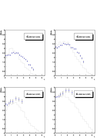
FIG. 3.: Final pseudorapidity distributions (quarks only) for a $p$$-$$\bar{p}$ reaction at
$\sqrt{s}=200,630,900\text{ and }1800\text{ GeV}$. The histograms are the PCPC results. The data points are the experimental $\frac{dN_{ch}}{d\eta}$ (from [45] for 200 GeV, 900 GeV, and [46] for 630 GeV, 1800 GeV, resp.).

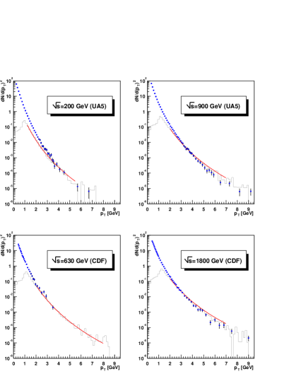
FIG. 4.: Distributions of final transverse momenta for a $p$$-$$\bar{p}$ reaction at
$\sqrt{s}=200,630,900\text{ and }1800\text{ GeV}$. Note the rapidity cut: only particles with $|y|<1$ are included. The histograms are the PCPC results. The data points (including the fit lines through them) are the experimental $\frac{dN_{ch}}{dp_{\,\mathsf{T}}}$ (from [47] and [48]).

 

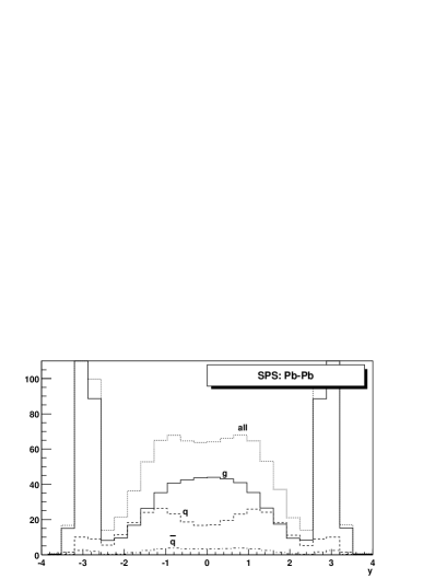
FIG. 5.: Final parton rapidity distributions for a S$-$S reaction ($\sqrt{s}=2\times 9.7$ A$\cdot$GeV, top frame) and Pb$-$Pb ($\sqrt{s}=2\times 8.6$ A$\cdot$GeV, bottom frame). Shown are the separate contributions of gluons ($g$), up and down quarks ($q$) and up and down antiquarks ($\bar{q}$).

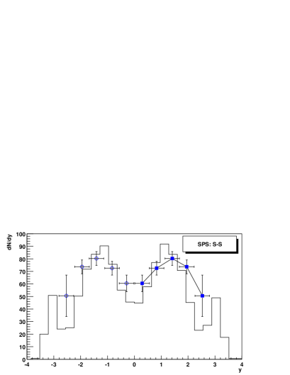
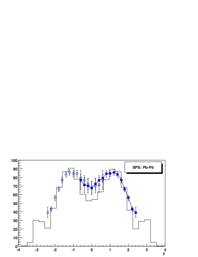
FIG. 6.: Final rapidity distributions of ‘net baryons’ (arbitrary units) for a S$-$S reaction ($\sqrt{s}=2\times 9.7$ A$\cdot$GeV, top frame) and Pb$-$Pb ($\sqrt{s}=2\times 8.6$ A$\cdot$GeV, bottom frame). The histograms are results of the PCPC simulation, the data point and their error bars are from [52].

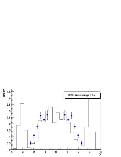
FIG. 7.: Rapidity distributions (arbitrary units) of final antistrange quarks for a S$-$S reaction at $\sqrt{s}=2\times 9.7$ A$\cdot$GeV. The experimental data points are from [53].

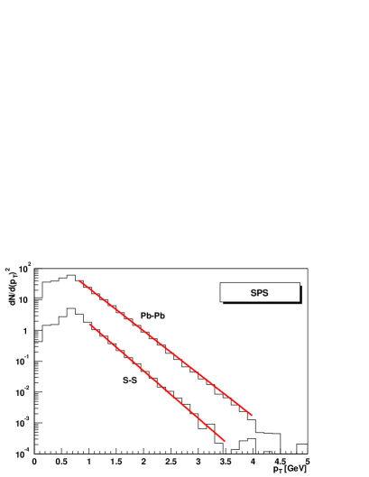
FIG. 8.: Distributions of final parton transverse momenta for S$-$S ($\sqrt{s}=2\times 9.7$ A$\cdot$GeV) and (Pb$-$Pb ($\sqrt{s}=2\times 8.6$ A$\cdot$GeV). The solid lines merely serve to show to what extent the distributions are exponential.

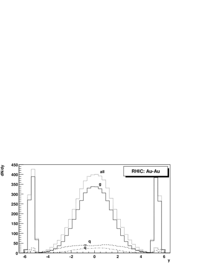
FIG. 9.: Final parton rapidity distributions for Au$-$Au reactions at RHIC. Shown are the total partons and the separate contributions of gluons ($g$), quarks and antiquarks.

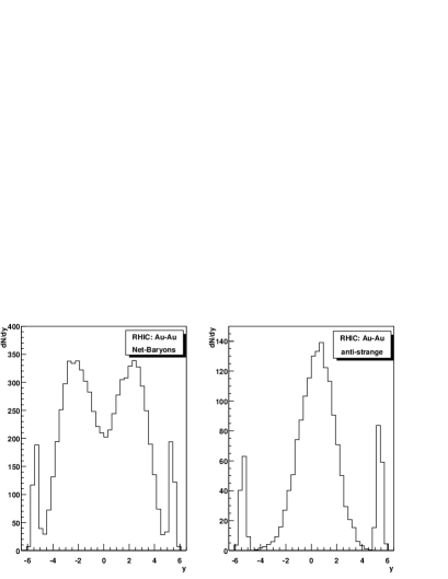
FIG. 10.: Final rapidity distributions of ‘net baryons’ (left frame) and antistrange quarks (right frame) for Au$-$Au reactions at RHIC.

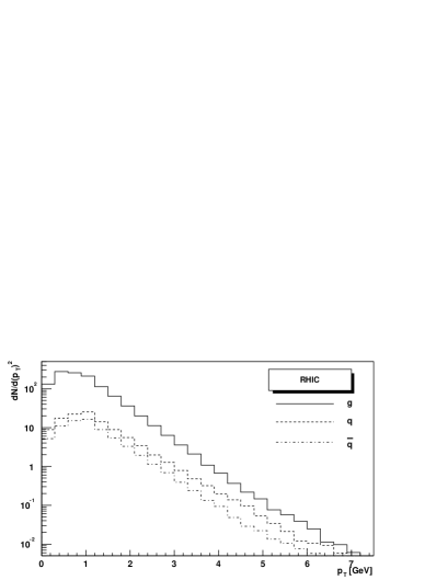
FIG. 11.: Distributions of final parton transverse momenta for Au$-$Au reactions at RHIC.

process	$|{\mathcal{M}}/g^{2}|^{2}$
$gg\rightarrow gg$	$G_{0}(s,t,u)$
$gg\rightarrow q\bar{q}$	$G_{3}(s,t,u;m)$
$\!\!\begin{array}[]{l}qg\rightarrow qg,\\ \bar{q}g\rightarrow\bar{q}g\end{array}$	$\left\langle\textstyle\frac{8}{3}\displaystyle\right\rangle G_{3}(t,s,u;m)$
$\!\!\begin{array}[]{l}qq\rightarrow qq,\\ \bar{q}\bar{q}\rightarrow\bar{q}\bar{q}\end{array}$	$\!\!\begin{array}[]{r}G_{1}(s,t,u;m,m)+G_{1}(s,u,t;m,m)\\ +G_{2}(s,t,u;m)\end{array}$
$q\bar{q}\rightarrow q\bar{q}$	$\!\!\begin{array}[]{r}G_{1}(u,s,t;m,m)+G_{1}(u,t,s;m,m)\\ +G_{2}(u,s,t;m)\end{array}$
$q\bar{q}\rightarrow q^{\prime}{\bar{q}}^{\prime}$	$G_{1}(u,s,t;m,m^{\prime})$
$q\bar{q}\rightarrow gg$	$\left\langle\textstyle\frac{64}{9}\displaystyle\right\rangle G_{3}(s,t,u;m)$
$\!\!\begin{array}[]{l}qq^{\prime}\rightarrow qq^{\prime},\\ q{\bar{q}}^{\prime}\rightarrow q{\bar{q}}^{\prime},\\ \bar{q}{\bar{q}}^{\prime}\rightarrow\bar{q}{\bar{q}}^{\prime}\end{array}$	$G_{1}(s,t,u;m,m^{\prime})$

TABLE I.: Matrix elements (with the coupling constant factored out) for the partonic processes $ab\rightarrow cd$. The numerical factors in brackets are due to different colour averages.

$\begin{array}[]{l}\frac{4}{3}\frac{1+z^{2}}{1-z}\\ \frac{4}{3}\frac{1+(1-z)^{2}}{z}\\ \text{{6}}\,\frac{[1-z(1-z)]^{2}}{z(1-z)}\\ \textstyle\frac{1}{2}\displaystyle\left[z^{2}+(1-z)^{2}\right]\end{array}\text{\qquad for }\left\{\begin{array}[]{l}q\rightarrow qg\\ q\rightarrow gq\\ g\rightarrow gg\\ g\rightarrow q\bar{q}\end{array}\right.$

TABLE II.: Altarelli-Parisi splitting functions $P_{a\rightarrow bc}(z)$ . From [42].

Flavor $b$	Flavor $a$
$g$	$g$
	$u,\bar{u},d,\bar{d},s,\bar{s}\ldots$
$u(\bar{u})$	$u(\bar{u})$
	$g$
$d(\bar{d})$	$d(\bar{d})$
	$g$
$s(\bar{s})$	$s(\bar{s})$
	$g$
$\vdots$	$\vdots$

TABLE III.: Flavor generation in the parton evolution. A parton with flavor $b$ may be radiated from a parton with flavor $a$. The list includes all possible QCD branchings.

		$p$$-$$\bar{p}$				S$-$S	Pb$-$Pb	Au$-$Au
$\sqrt{s}$	[A$\cdot$GeV]	200	615	900	1800	9.7	8.6	100
$x_{\text{min}}$		0.01	0.003	0.002	0.001	0.1	0.12
${Q_{0}}^{2}$	[$\text{GeV}^{2}$]	5.3	9.8	11.7	16.6	1.6	1.3	5.3
${Q_{\text{min}}}^{2}$	[$\text{GeV}^{2}$]	1.73	2.36	2.60	3.14	0.92	0.89	1.73

TABLE IV.: Values of various parameters used in the numerical computations (the meaning of these parameters is explained in Sects. III and IV).