The spin correlation in top quark production:
QCD corrections vs anomalous couplings

Abstract

We discuss top quark production and its subsequent decay at lepton colliders including both QCD corrections and anomalous $\gamma/Z-t\bar{t}$ couplings. The off-diagonal spin basis for the top and anti-top quarks is shown to be useful to probe the anomalous couplings.

1 Introduction

Since the discovery of the top quark, with a large mass [1], its properties have been widely discussed to obtain a better understanding of the electroweak symmetry breaking and to search for hints of physics beyond the standard model (SM). It has been known that top quarks decay before hadronization [2]. Therefore there will be sizable angular correlations between the decay products of the top quark and the spin of the top quark [3]. Based on this observation, it is expected that we can either test the SM or obtain some signal from new physics by investigating the angular distributions of the decay products from polarized top quarks.

Applying the narrow width approximation to the top quarks, we can discuss the production process and decay process separately. There are many papers on the spin correlations in top quark production and also the angular distributions of decay products by combining the production with the decay process [4]. Although it was common to use the helicity basis to decompose the top quark spin, it has been pointed out by Mahlon, Parke and Shadmi [5] that there is a more optimal decomposition of the top quark spin depending on the process and the center of energy.

On the other hand, there are also many detailed studies on the effects of new operators which might come from physics beyond the SM [6]. The fact that the SM is consistent with the data within the present experimental accuracy tells us that the size of the effects of new physics is at most comparable to or smaller than the radiative corrections in the SM. Therefore it might be important to estimate also the effects of the SM radiative corrections.

In this talk, we will discuss the QCD corrections to the spin correlations in the top quark productions at lepton colliders and present the angular distribution of the decay product including both the QCD corrections and the so-called anomalous couplings for the $\gamma/Z-t\bar{t}$ interaction.

2 QCD corrections to the spin correlation

We first discuss the QCD correction to the spin dependent cross section for the top quark production from the polarized $e^{-}e^{+}$ [7]. The spin direction of the top quark is parameterized by $\xi$ as in Fig.1 at the top quark rest frame. The anti-top quark spin state is similarly defined by the same $\xi$.

Figure 1: The spin vector ${\bf s}_{t}$ for the top quark is defined in the top quark rest frame.

The tree level cross section is easily calculated to be,

$$\frac{d\sigma}{d\cos\theta^{*}}\left(e^{-}_{L}e^{+}_{R}\to t_{\uparrow}\bar{t}_{\uparrow}\right)=\frac{d\sigma}{d\cos\theta^{*}}\left(e^{-}_{L}e^{+}_{R}\to t_{\downarrow}\bar{t}_{\downarrow}\right)$$

$$=\left(\frac{3\pi\alpha^{2}}{2s}\beta\right)\,|(A_{LR}\cos\xi-B_{LR}\sin\xi)|^{2}$$ (1)

$$\frac{d\sigma}{d\cos\theta^{*}}\left(e^{-}_{L}e^{+}_{R}\to t_{\uparrow}\bar{t}_{\downarrow}\ {\rm or}\ t_{\downarrow}\bar{t}_{\uparrow}\right)$$

$$=\left(\frac{3\pi\alpha^{2}}{2s}\beta\right)\,|(A_{LR}\sin\xi+B_{LR}\cos\xi\pm D_{LR})|^{2}$$

where

$$A_{LR}=\Bigl{[}(f_{LL}+f_{LR})\sqrt{1-\beta^{2}}\sin\theta^{*}\Bigr{]}/2$$

$$B_{LR}=\Bigl{[}f_{LL}(\cos\theta^{*}+\beta)+f_{LR}(\cos\theta^{*}-\beta)\Bigr{]}/2$$

$$D_{LR}=\Bigl{[}f_{LL}(1+\beta\cos\theta^{*})+f_{LR}(1-\beta\cos\theta^{*})\Bigr{]}/2$$

$$f_{IJ}=-Q_{t}+\frac{Q^{e}_{I}\,Q^{t}_{J}}{\sin^{2}\theta_{W}}\frac{s}{s-M_{Z}^{2}}$$

Here $\alpha$ is the QED fine structure constant, $\theta^{*}(\beta)$ is the scattering angle (the speed) of top quark in the zero momentum frame and $Q^{e}_{I}(Q^{t}_{J})$ is the electron (top quark) coupling to the Z boson. $M_{Z}$ is the Z-boson mass and $\theta_{W}$ is the Weinberg angle. From eq.(1), one can see that the choice $\tan\xi=A_{LR}/B_{LR}$ results in a large asymmetry. This spin basis is called “off-diagonal”  basis [5]. Since $|f_{LL}|\gg|f_{LR}|$ numerically, it turns out that only one spin configuration dominates the cross section. On the other hand, in the helicity basis ($\cos\xi=\pm 1$) all configurations significantly contribute to the cross section.

The QCD corrections might modify the tree level results since they induce an anomalous $\gamma/Z$ magnetic moment for the top quark and allow for single real gluon emission. Since the top and anti-top quarks are not necessarily produced back to back at the one loop level, we discuss the single spin correlation. Here we show only the numerical results of our calculations [7].

Table I summarizes the strong coupling constant $\alpha_{s}$, $\beta$, and the tree and ${\cal O}(\alpha_{s})$ level total cross sections in $e^{-}_{L}e^{+}$ scattering.

$\sqrt{s}$	$400$ GeV	$800$ GeV
$\beta$	$0.484$	$0.899$
$\alpha_{s}(s)$	$0.0980$	$0.0910$
$\sigma_{Total}$ Tree (pb)	$0.8707$	$0.3531$
$\sigma_{Total}$ $\cal{O}\mit(\alpha_{s})$ (pb)	$1.113$	$0.3734$

Table  I: The values of $\beta$, $\alpha_{s}$, tree and next to leading order cross sections.

To see the effects of the QCD corrections to the spin correlation, we write the cross section as a sum of two terms.

$$\frac{d\sigma}{d\cos\theta^{*}}(e_{L}^{-}e_{R}^{+}\to t_{\uparrow\downarrow}X)$$

$$= (1+\kappa)\,\frac{d\sigma^{0}}{d\cos\theta^{*}}(e_{L}^{-}e_{R}^{+}\to t_{\uparrow\downarrow}X)$$

$$\qquad\qquad+\frac{d\sigma^{R}}{d\cos\theta^{*}}(e_{L}^{-}e_{R}^{+}\to t_{\uparrow\downarrow}X)$$

The first term is a part which is proportional to the tree level cross section. Therefore, $1+\kappa$ is simply the multiplicative enhancement (K-) factor. Whereas the second term give the ${\cal O}(\alpha_{s})$ deviations to the spin correlations. Our numerical studies show that the ${\cal O}(\alpha_{s})$ QCD corrections enhance the tree level result (the first term) and only slightly modifies the spin orientation of the produced top quark (the second term). The ratio of the second term to the first one is of order a few percent. In the kinematical region where the emitted gluon has small energy, it is natural to expect that the real gluon emission effects introduce only a multiplicative correction to the tree level result. Therefore only “hard” gluon emission could possibly modify the top quark spin orientation. What we have found, by explicit calculation, is that this effect is numerically very small. In Table II, we give the fraction of the top quarks in the subdominant spin configuration with $K$ factor for $e^{-}_{L}e^{+}$ scattering,

$$\sigma\left(e^{-}_{L}e^{+}\rightarrow t_{\downarrow\uparrow}X(\bar{t}{\rm~{}or~{}}\bar{t}g)\right)/\sigma^{Total}_{L}$$

for the helicity and off-diagonal bases. These results suggest that the soft gluon approximation (SGA) will be sufficient to estimate the 1-loop QCD corrections. Actually, we have checked that the SGA can reproduce the full results quite accurately by choosing an appropriate cut off $\omega_{\rm max}$ for the soft gluon. The difference between the SGA using this $\omega_{\rm max}$ and the full 1-loop correction is smaller than the expected size of the 2-loop corrections.

$\sqrt{s}$ (GeV)	$\kappa$	Helicity	Off-Diagonal
		0.336	0.00124
400	0.278
		0.332	0.00150
		0.168	0.0265
800	0.057
		0.165	0.0319

Table  II: The fraction of the $e^{-}_{L}e^{+}$ cross section in the subdominant spin. The upper (lower) line corresponds to the tree (one-loop) level.

3 Decay distribution with anomalous coupling

Although the QCD correction to the top quark production is not so large, it should be included to detect “small” signals from possible new physics beyond the SM. We analyze the top quark production and its subsequent decay at lepton colliders including both QCD corrections and anomalous $\gamma/Z-t\bar{t}$ couplings.

The process we are considering now is, in principle, a very complicated $e^{-}e^{+}\to 6$ one. However, it has been known that the narrow width approximation for the top quark, which is valid for $\Gamma_{t}\ll m_{t}$ (1.02 $\leq\Gamma_{t}\leq$ 1.56 GeV for 160 $\leq m_{t}\leq$ 180 GeV), makes the situation very simple. Namely, we can separate the physics into the top production and the decay density matrices [8].

Let us first discuss the top quark production (density matrix). We assume a general form for the $t$-$\bar{t}$-$Z/\gamma$ vertex as,

$$\Gamma^{V}_{\mu} = g^{V}\left\{\gamma_{\mu}\left[Q_{L}^{V}\omega_{-}+Q_{R}^{V}\omega_{+}\right]\right.$$ (2)

$$\qquad+\left.\frac{(t-{\bar{t}})_{\mu}}{2m_{t}}\left[G_{L}^{V}\omega_{-}+G_{R}^{V}\omega_{+}\right]\right\}$$

where $t,\bar{t}$ are momenta of the top and anti-top quarks, $m_{t}$ is the top mass, $\omega_{-}/\omega_{+}$ is the left/right projection operator, and $V=Z$ or $\gamma$. For the $e$-$\bar{e}$-$Z/\gamma$ vertex, we use the well established SM interaction. At the tree level in the SM, the coupling constants $G^{V}_{L,R}$ are zero. The combination of form factors $G^{\gamma,Z}_{R}+G^{\gamma,Z}_{L}\equiv f_{2}^{\gamma,Z}$ is induced even at the one-loop level in the SM. Whereas, another combination $G^{\gamma,Z}_{R}-G^{\gamma,Z}_{L}\equiv if_{3}^{\gamma,Z}$ which is related to a CP violating interaction, called electric and weak dipole form factors (EDM and WDM) appears as, at least, the two-loop order effect. Thus they are negligibly small and non-zero value of $f_{3}^{\gamma,Z}$ is considered to be a contribution from new physics beyond the SM. We presume some non-zero value for $f_{3}^{\gamma,Z}$ and consider the top production and its decay. The QCD one-loop correction is easily incorporated into this analysis if one remembers that the one loop effect is very well approximated by the SGA. In the SGA, QCD effects can be expressed by the modified $t$-$\bar{t}$-$Z/\gamma$ vertex [7], eq.(2).

$$Q_{LR}^{V}\sim 1+{\cal O}(\alpha_{s})\quad,\quad G_{R}^{V}+G_{L}^{V}\sim{\cal O}(\alpha_{s})$$

$$G_{R}^{V}-G_{L}^{V}={\cal O}(\alpha_{s}^{2})\sim 0.$$

The top quark production amplitudes now read,

$$M(e_{L}^{-}e_{R}^{+}\rightarrow t_{\uparrow}\bar{t}_{\uparrow},t_{\downarrow}\bar{t}_{\downarrow})$$

$$= \mp 4\pi\alpha\left[\hat{A}_{LR}\cos\xi-\hat{B}_{LR}\sin\xi\pm iE_{LR}\right]$$

$$M(e_{L}^{-}e_{R}^{+}\rightarrow t_{\uparrow}\bar{t}_{\downarrow},t_{\downarrow}\bar{t}_{\uparrow})$$

$$= \ \ 4\pi\alpha\left[\hat{A}_{LR}\sin\xi+\hat{B}_{LR}\cos\xi\pm\hat{D}_{LR}\right].$$

where we have chosen the phases of spinors to be real. The coefficients with  $\hat{}$   receive the contribution from the QCD corrections,

$$\hat{C}_{LR}=C_{LR}+{\cal O}(\alpha_{s}).$$

For the explicit expressions, see ref.[7]. The function $E_{LR}$ linearly depends on $f_{3}^{\gamma,Z}$ and is given by,

$$E_{LR}=\frac{1}{2}(h_{LL}-h_{LR})\frac{\beta\sin\theta^{*}}{\sqrt{1-\beta^{2}}}\ ,$$

with

$$h_{IJ}=-G^{\gamma}_{J}(t)+\frac{Q^{Z}_{I}(e)G^{Z}_{J}(t)}{\sin^{2}\theta_{W}}\frac{s}{s-M_{Z}^{2}}\ .$$

The problem now is how to detect the anomalous coupling in the top quark events. It is easily understood that the effects of the anomalous coupling on the top quark production cross sections should be small and undetectable since the anomalous coupling is assumed to be comparable to or smaller than the QCD correction in size and we already know the QCD correction itself to be small. Therefore we consider the angular distribution of top decay products which depends linearly on $f_{3}^{\gamma,Z}$.

In the decay process, we assume V-A interaction of the SM in $t$-$b$-$W$ vertex. We employ the semi-leptonic decay, $t\rightarrow bW\rightarrow b\bar{l}\nu$ for simplicity. Neglecting the mass of the final state fermions, the decay amplitude $D_{s_{t}}$ (for $t_{s_{t}}\to b\bar{l}\nu$) is known to be given by

$$D_{\uparrow} = \frac{2g^{2}V_{tb}\sqrt{b\cdot\nu~{}m_{t}E_{\bar{l}}}}{2\nu\cdot\bar{l}-M_{W}^{2}+iM_{W}\Gamma_{W}}\cos\frac{\theta_{\bar{l}}}{2}$$

$$D_{\downarrow} = \frac{2g^{2}V_{tb}\sqrt{b\cdot\nu~{}m_{t}E_{\bar{l}}}}{2\nu\cdot\bar{l}-M_{W}^{2}+iM_{W}\Gamma_{W}}\sin\frac{\theta_{\bar{l}}}{2}e^{-i\phi_{\bar{l}}}$$

where the names of final particles are used as substitute for their momenta. $M_{W}$ and $V_{tb}$ are the masses of the W boson and the Cabbibo–Kobayashi–Maskawa (CKM) matrix.

Figure 2: The definition of polar and azimuthal angles.

The polar and azimuthal angles of the $\bar{l}$ momentum ($\theta_{\bar{l}},\phi_{\bar{l}}$) are defined in the top quark rest frame, in which $z$-axis coincides with the chosen spin axis $s_{t}$ and $x-z$ is the production plane, Fig.2. We have a similar expression $\bar{D}_{\uparrow\downarrow}$ also for the anti-top quark decay.

Now, the differential cross-section for the process $e^{-}e^{+}\to t\bar{t}$ followed by the decays $t\to X_{t}\,,\,\bar{t}\to\bar{X}_{t}$ is described in terms of the production and decay density matrices $\rho_{s_{t}\bar{s}_{t},s^{\prime}_{t}\bar{s}^{\prime}_{t}}$  ,  $\tau_{s_{t}s^{\prime}_{t}}$ and $\bar{\tau}_{\bar{s}_{t}\bar{s}^{\prime}_{t}}$ as,

$$d\sigma\left(e^{-}e^{+}\to t\bar{t}\to X_{t}\bar{X}_{t}\right)$$

$$\propto \sum_{s_{t},\bar{s}_{t},s^{\prime}_{t},\bar{s}^{\prime}_{t}}\rho_{s_{t}\bar{s}_{t},s^{\prime}_{t}\bar{s}^{\prime}_{t}}\tau_{s_{t}s^{\prime}_{t}}\bar{\tau}_{\bar{s}_{t}\bar{s}^{\prime}_{t}}dL,$$

where $dL$ is the phase space of the final particles and the density matrices can be obtained from eqs.(LABEL:proamp) and (LABEL:eq:D2) [8].

$$\rho_{s_{t}\bar{s}_{t},s^{\prime}_{t}\bar{s}^{\prime}_{t}}=M_{s_{t}\bar{s}_{t}}M^{\ast}_{s^{\prime}_{t}\bar{s}^{\prime}_{t}}$$

$$\tau_{s_{t}s^{\prime}_{t}}\propto D_{s_{t}}D^{\ast}_{s^{\prime}_{t}}\propto\left(\begin{array}[]{cc}1+\cos\theta_{\bar{l}}&\sin\theta_{\bar{l}}e^{i\phi_{\bar{l}}}\\ \sin\theta_{\bar{l}}e^{-i\phi_{l}}&1-\cos\theta_{\bar{l}}\\ \end{array}\right)_{s_{t}s^{\prime}_{t}}$$

$\bar{\tau}_{\bar{s}_{t}\bar{s}^{\prime}_{t}}$ is also given by the similar expression. When we calculated the production density matrix, we have kept terms up to linear in $\alpha_{s}$ and $f_{3}^{\gamma,Z}$ for the consistency of our approximation. We have also applied the narrow width approximation for the W boson in eq.(LABEL:eq:D2) to derive the above result. From this expression, we see that there are terms which linearly depend on $f_{3}^{\gamma,Z}$ in the angular distributions of the charged leptons and the interference terms between amplitudes for different spin configuration play an important role.

Here we take an advantage of the freedom for the choice of the spin basis to detect the effect of the anomalous couplings. Note that the differential cross section itself is (should be) independent of the choice of the spin basis. However, the “choice of the variables”  can depend on the spin basis. We have calculated the angular distribution of $\bar{l}$ in the top quark decay after integrating out other variables. We plot the $\theta_{\bar{l}}-\phi_{\bar{l}}$ correlations both in the helicity (Fig.3) and the off-diagonal basis (Fig.4). We set $\sqrt{s}=400\ GeV$ and assume $f_{3}^{\gamma,Z}=0.2$ just for an illustration. The both figures are for $\cos\theta^{*}=0$. However the pattern of the correlation is essentially the same for all scattering angles. One can see that it is very hard to identify the effects of the anomalous couplings in Fig. 3, This situation changes drastically if we take the off-diagonal basis (Fig. 4). As the SM result produces almost no azimuthal angular dependence in this basis (these azimuthal angular dependencies are caused by interferences effects in a given spin basis and these are very small in the off-diagonal basis), we recognize the effect of the anomalous coupling as a deviation from the flat distribution. For the value of the anomalous coupling we have chosen, these new interactions change the shape nearly by 10%.

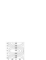
Figure 3: The double differential cross section $d^{2}\sigma/d\cos\theta_{\bar{l}}d\phi_{\bar{l}}$ in the helicity basis. The left (right) figure correspond to the cross section without (with) the anomalous $f_{3}^{\gamma,Z}$ coupling. Vertical and horizontal axes correspond to the azimuthal $\phi_{\bar{l}}$ and the polar angle $\cos\theta_{\bar{l}}$, respectively.

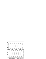
Figure 4: The double differential cross section in the off-diagonal basis. The left (right) figure correspond to the cross section without (with) the anomalous $f_{3}^{\gamma,Z}$ coupling. The axes are the same as in Fig.3

In order to show the effect of the $f_{3}^{\gamma,Z}$ more clearly, we partially integrate the cross section over the azimuthal angle and define the azimuthal asymmetry. Let $\sigma^{1,2}$ denote the partially integrated cross-sections over the azimuthal angle,

$$\sigma^{1}(\theta^{*}) = \int_{0}^{\pi}d\phi_{l}\left(\frac{d\sigma}{d\cos\theta^{*}d\phi_{l}}\right)\ ,$$

$$\sigma^{2}(\theta^{*}) = \int_{\pi}^{2\pi}d\phi_{\bar{l}}\left(\frac{d\sigma}{d\cos\theta^{*}d\phi_{l}}\right)$$

where other variables have been integrated out already. We define the azimuthal asymmetry in order to pull out the effect of anomalous interactions,

$${\cal A}(\theta^{*})=\frac{\sigma^{2}(\theta^{*})-\sigma^{1}(\theta^{*})}{\sigma^{2}(\theta^{*})+\sigma^{1}(\theta^{*})}.$$

We plot the asymmetry as a function of $\cos\theta^{*}$ in Fig.5 at $\sqrt{s}=400GeV$ for the $e^{+}_{R}e^{-}_{L}$ and $e^{+}_{L}e^{-}_{R}$ annihilation.

Figure 5: Azimuthal asymmetry as a function of $\cos\theta^{*}$ in the off-diagonal basis.

In this figure, the dot-dashed line comes from the SM (with QCD corrections) and others from anomalous couplings. At the SM tree level, the asymmetry is exactly zero and the QCD radiative corrections induce a numerically negligible asymmetry as shown in Fig.6. The asymmetry strongly depends on the value and the sign of $f_{3}^{\gamma,Z}$. In the case of $e^{+}_{R}e^{-}_{L}$, the effects of the anomalous interactions $f_{3}^{\gamma}$ and $f_{3}^{Z}$ are additive and have a larger asymmetry when their signs are the same. But when their signs are opposite, these effects become subtractive and lead to a smaller asymmetry. This feature changes in the case of $e^{+}_{L}e^{-}_{R}$. In the off-diagonal basis, the anomalous couplings produce the asymmetry of the order 10%. In the helicity basis, however, the deviation from the SM is only around 1.5% since there exists some amount of asymmetry already in the SM.

Figure 6: Azimuthal asymmetry induced by the QCD correction in the off-diagonal basis.

4 Conclusion

We have studied the top quark pair production and subsequent decays at lepton colliders. First, we reported that the contribution of QCD corrections is mainly just the enhancement of the tree level result (K-factor) and does not change the spin configuration of produced top quarks. For a realistic next lepton colliders, let us say $\beta\sim 0.5$, the helicity basis is a poor choice since all spin configurations contribute to the production process. This means that there is a significant interference between the intermediate spin states. On the other hand, the off-diagonal basis is a good choice since the contribution from some spin states is zero or negligible even after including the QCD corrections. This small interference makes the correlations between decay products and the top spin very strong. Using this advantage, we analyzed, secondly, the angular dependence of the decay product of the top quark including both the QCD corrections and the anomalous couplings. We have shown that the asymmetry amount to the order of 10% in the off-diagonal basis with chosen parameters which may be detectable.

Although we have considered the anomalous couplings only for the production process and showed the results for their particular values, the inclusion of new effects to the decay process and more detailed phenomenological analyses for various choices of the new interactions are quite straightforward exercises.

References

- [1] F. Abe et al., CDF Collab., Phys. Rev. Lett. 74 (1995) 2626; S. Abachi et al., D0 Collab., Phys. Rev. Lett. 74 (1995) 2632.
- [2] I. Bigi, Y. Dokshitzer, V. Khoze, J. Kühn and P. Zerwas, Phys. Lett. B181 (1986) 157.
- [3] J. H. Kühn, Nucl. Phys. B237 (1984) 77; M. Jeżabek and J. H. Kühn, Phys. Lett. B329 (1994) 317, and references therein.
- [4] G. Mahlon and S. Parke, hep-ph/0001201; and references therein.
- [5] G. Mahlon and S. Parke, Phys. Rev. D53 (1996) 4886; Phys. Lett. B411 (1997) 173; S. Parke and Y. Shadmi, Phys. Lett. B387 (1996) 199.
- [6] see e.g. T. Torma, hep-ph/9912281; S. M. Lietti and H. Murayama, hep-ph/0001304; S. D. Rindani, hep-ph/0002006; B. Grzadkowski and Z. Hioki, hep-ph/0003294; and references therein.
- [7] J. Kodaira, T. Nasuno and S. Parke, Phys. Rev. D59 (1999) 014023.
- [8] M. Jezabek and J. H. Kühn, Nucl. Phys. B320 (1989)20; A. Czarnecki, M. Jeżabek and J. H. Kühn, ibid. B427 (1994) 3; B. Lampe, hep-ph/9801346, MPI-PHT Report No.98-07.