IISc-CTS-12/99

ZU-TH 10/00

BUTP-99/33

Roy equation analysis of $\pi\pi$ scattering

May 30, 2000

B. Ananthanarayan^a, G. Colangelo^b, J. Gasser^c and H. Leutwyler^c

${}^{a}\,$Centre for Theoretical Studies, Indian Institute of Science

Bangalore, 560 012 India

${}^{b}\,$Institute for Theoretical Physics, University of Zürich

Winterthurerstr. 190, CH-8057 Zürich, Switzerland

${}^{c}\,$Institute for Theoretical Physics, University of Bern

Sidlerstr. 5, CH-3012 Bern, Switzerland

We analyze the Roy equations for the lowest partial waves of elastic $\pi\pi$ scattering. In the first part of the paper, we review the mathematical properties of these equations as well as their phenomenological applications. In particular, the experimental situation concerning the contributions from intermediate energies and the evaluation of the driving terms are discussed in detail. We then demonstrate that the two $S$-wave scattering lengths $a_{0}^{0}$ and $a_{0}^{2}$ are the essential parameters in the low energy region: Once these are known, the available experimental information determines the behaviour near threshold to within remarkably small uncertainties. An explicit numerical representation for the energy dependence of the $S$- and $P$-waves is given and it is shown that the threshold parameters of the $D$- and $F$-waves are also fixed very sharply in terms of $a_{0}^{0}$ and $a^{2}_{0}$. In agreement with earlier work, which is reviewed in some detail, we find that the Roy equations admit physically acceptable solutions only within a band of the ($a_{0}^{0}$,$a_{0}^{2}$) plane. We show that the data on the reactions $e^{+}e^{-}\rightarrow\pi\,\pi$ and $\tau\rightarrow\pi\,\pi\,\nu$ reduce the width of this band quite significantly. Furthermore, we discuss the relevance of the decay $K\rightarrow\pi\,\pi\,e\,\nu$ in restricting the allowed range of $a_{0}^{0}$, preparing the grounds for an analysis of the forthcoming precision data on this decay and on pionic atoms. We expect these to reduce the uncertainties in the two basic low energy parameters very substantially, so that a meaningful test of the chiral perturbation theory predictions will become possible.

Pacs:	11.30.Rd, 11.55.Fv, 11.80.Et, 13.75.Lb
Keywords:	Roy equations, Dispersion relations, Partial wave analysis,
	Meson-meson interactions, Pion-pion scattering, Chiral symmetries

1 Introduction

The present paper deals with the properties of the $\pi\pi$ scattering amplitude in the low energy region. Our analysis relies on a set of dispersion relations for the partial wave amplitudes due to Roy [1]. These equations involve two subtraction constants, which may be identified with the $S$-wave scattering lengths, $a_{0}^{0}$ and $a_{0}^{2}$. We demonstrate that the subtraction constants represent the essential parameters in the low energy region – once these are known, the Roy equations allow us to calculate the partial waves in terms of the available data, to within small uncertainties. Given the strong dominance of the two $S$-waves and of the $P$-wave, it makes sense to solve the equations only for these, using experimental as well as theoretical information to determine the contributions from higher energies and from the higher partial waves. More specifically, we solve the relevant integral equations on the interval $2M_{\pi}<\sqrt{s}<0.8\,\mbox{GeV}$. One of the main results of this work is an accurate numerical representation of the $S$- and $P$-waves for a given pair of scattering lengths $a_{0}^{0}$ and $a_{0}^{2}$.

Before describing the outline of the present paper, we review previous work concerning the Roy equations. Roy’s representation [1] for the partial wave amplitudes $t^{I}_{l}$ of elastic $\pi\pi$ scattering reads

$$t_{\ell}^{I}(s)=k_{\ell}^{I}(s)+\sum_{I^{\prime}=0}^{2}\sum_{\ell^{\prime}=0}^{\infty}\int_{4M_{\pi}^{2}}^{\infty}ds^{\prime}\,K_{\ell\ell^{\prime}}^{II^{\prime}}(s,s^{\prime})\,\mbox{Im}\,t_{\ell^{\prime}}^{I^{\prime}}(s^{\prime})\,,$$ (1.1)

where $I$ and $\ell$ denote isospin and angular momentum, respectively and $k^{I}_{\ell}(s)$ is the partial wave projection of the subtraction term. It shows up only in the $S$- and $P$-waves,

$$k^{I}_{\ell}(s) \!\!\!\!= \!\!\!\!a_{0}^{I}\,\delta_{\ell}^{0}+\frac{s-4M_{\pi}^{2}}{4M_{\pi}^{2}}\,(2a_{0}^{0}-5a_{0}^{2})\,\left(\frac{1}{3}\,\delta_{0}^{I}\,\delta_{\ell}^{0}+\frac{1}{18}\,\delta_{1}^{I}\,\delta_{\ell}^{1}-\frac{1}{6}\,\delta_{2}^{I}\,\delta^{0}_{\ell}\right).$$ (1.2)

The kernels $K_{\ell\ell^{\prime}}^{II^{\prime}}(s,s^{\prime})$ are explicitly known functions (see appendix A). They contain a diagonal, singular Cauchy kernel that generates the right hand cut in the partial wave amplitudes, as well as a logarithmically singular piece that accounts for the left hand cut. The validity of these equations has rigorously been established on the interval $-\,4M_{\pi}^{2}<s<60M_{\pi}^{2}$.

The relations (1.1) are consequences of the analyticity properties of the $\pi\pi$ scattering amplitude, of the Froissart bound and of crossing symmetry. Combined with unitarity, the Roy equations amount to an infinite system of coupled, singular integral equations for the phase shifts. The integration is split into a low energy interval $4M_{\pi}^{2}<s^{\prime}<s_{0}$ and a remainder, $s_{0}<s^{\prime}<\infty$. We refer to $s_{0}$ as the matching point, which is chosen somewhere in the range where the Roy equations are valid. The two $S$-wave scattering lengths, the elasticity parameters below the matching point and the imaginary parts above that point are treated as an externally assigned input. The mathematical problem consists in solving Roy’s integral equations with this input.

Soon after the original article of Roy [1] had appeared, extensive phenomenological applications were performed [2]–[8], resulting in a detailed analysis and exploitation of the then available experimental data on $\pi\pi$ scattering. For a recent review of those results, we refer the reader to the article by Morgan and Pennington [9]. Parallel to these phenomenological applications, the very structure of the Roy equations was investigated. In [11], a family of partial wave equations was derived, on the basis of manifestly crossing symmetric dispersion relations in the variables $s\,t+t\,u+u\,s$ and $s\,t\,u$. Each set in this family is valid in an interval $s_{0}<s<s_{1}$, and the union of these intervals covers the domain $-28M_{\pi}^{2}\leq{\mbox{Re}}\,\,s\leq 125.3M_{\pi}^{2}$ (for a recent application of these dispersion relations, see [12]). Using hyperbolae in the plane of the above variables, Auberson and Epele [13] proved the existence of partial wave equations up to ${\mbox{Re}}\,\,s=165M_{\pi}^{2}$. Furthermore, the manifold of solutions of Roy’s equations was investigated, in the single channel [14]–[16] as well as in the coupled channel case [17]. In the late seventies, Pool [18] provided a proof that the original, infinite set of integral equations does have at least one solution for $\sqrt{\rule[1.00006pt]{0.0pt}{5.0pt}s_{0}}<4.8\,M_{\pi}$, provided that the driving terms are not too large, see also [19]. Heemskerk and Pool also examined numerically the solutions of the Roy equations, both by solving the $N$ equation [19] and by using an iterative method [20].

It emerged from these investigations that – for a given input of $S$-wave scattering lengths, elasticity parameters and imaginary parts – there are in general many possible solutions to the Roy equations. This non-uniqueness is due to the singular Cauchy kernel on the right hand side of (1.1). In order to investigate the uniqueness properties of the Roy system, one may – in a first step – keep only this part of the kernels, so that the integral equations decouple: one is left with a single channel problem, that is a single partial wave, which, moreover, does not have a left hand cut. This mathematical problem was examined by Pomponiu and Wanders, who also studied the effects due to the presence of a left hand cut [14]. Investigating the infinitesimal neighbourhood of a given solution, they found that the multiplicity of the solution increases by one whenever the value of the phase shift at the matching point goes through a multiple of $\pi/2$. Note that the situation for the usual partial wave equation is different: There, the number of parameters in general increases by two whenever the phase shift at infinity passes through a positive integer multiple of $\pi$, see for instance [21, 22] and references cited therein.

After 1980, interest in the Roy equations waned, until recently. For instance, in refs. [23] these equations are used to analyze the threshold parameters for the higher partial waves, relying on the approach of Basdevant, Froggatt and Petersen [5, 6]. The uncertainties in the values of $a_{0}^{0}$ and $a_{0}^{2}$ are reexamined in refs. [24]. In recent years, it has become increasingly clear, however, that a new analysis of the $\pi\pi$ scattering amplitude at low energies is urgently needed. New $K_{e4}$ experiments and a measurement of the combination $a_{0}^{0}-a_{0}^{2}$ based on the decay of pionic atoms are under way [25]–[29]. It is expected that these will significantly reduce the uncertainties inherent in the data underlying previous Roy equation studies, provided the structure of these equations can be brought under firm control. For this reason, the one-channel problem has been revisited in great detail in a recent publication [30], while the role of the input in Roy’s equations is discussed in ref. [31].

The main reason for performing an improved determination of the $\pi\pi$ scattering amplitude is that this will allow us to test one of the basic properties of QCD, namely the occurrence of an approximate, spontaneously broken symmetry: The symmetry leads to a sharp prediction for the two $S$-wave scattering lengths [32]–[40]. The prediction relies on the standard hypothesis, according to which the quark condensate is the leading order parameter of the spontaneously broken symmetry. Hence an accurate test of the prediction would allow us to verify or falsify that hypothesis [34]. First steps in this program have already been performed [35]–[39]. However, in the present paper, we do not discuss this issue. We follow the phenomenological path and ignore the constraints imposed by chiral symmetry altogether, in order not to bias the data analysis with theoretical prejudice. In a future publication, we intend to match the chiral perturbation theory representation of the scattering amplitude to two loops [40] with the phenomenological one obtained in the present work.

Finally, we describe the content of the present paper. Our notation is specified in section 2. Sections 3 and 4 contain a discussion of the background amplitude and of the driving terms, which account for the contributions from the higher partial waves and from the high-energy region. As is recalled in section 5, unitarity leads to a set of three singular integral equations for the two $S$-waves and for the $P$-wave. The uniqueness properties of the solutions to these equations are discussed in section 6, while section 7 contains a description of the experimental input used for energies between 0.8 and 2 GeV. In particular we also discuss the information concerning the $P$-wave phase shift, obtained on the basis of the $e^{+}e^{-}\rightarrow\pi\pi$ and $\tau\rightarrow\pi\pi\nu$ data. In section 8, we describe the method used to solve the integral equations for a given input. The resulting universal band in the ($a_{0}^{0}$,$a_{0}^{2}$) plane is discussed in section 9, where we show that, in the region below $0.8\,\mbox{GeV}$, any point in this band leads to a decent numerical solution for the three lowest partial waves. As discussed in section 10, however, the behaviour of the solutions above that energy is consistent with the input used for the imaginary parts only in part of the universal band – approximately the same region of the ($a_{0}^{0}$,$a_{0}^{2}$) plane, where the Olsson sum rule is obeyed (section 11). The solutions are compared with available experimental data in section 12, and in section 13, we draw our conclusions concerning the allowed range of $a_{0}^{0}$ and $a_{0}^{2}$. The other threshold parameters can be determined quite accurately in terms of these two. The outcome of our numerical evaluation of the scattering lengths and effective ranges of the lowest six partial waves as functions of $a_{0}^{0}$ and $a_{0}^{2}$ is given in section 14, while in section 15, we describe our results for the values of the phase shifts relevant for $K\rightarrow\pi\pi$. Section 16 contains a comparison with earlier work. A summary and concluding remarks are given in section 17.

In appendix A we describe some properties of the Roy kernels, which are extensively used in our work. The background from the higher partial waves and from the high energy tail of the dispersion integrals is discussed in detail in appendix B. In particular, we show that the constraints imposed by crossing symmetry reduce the uncertainties in the background, so that the driving terms can be evaluated in a reliable manner. In appendix C we discuss sum rules connected with the asymptotic behaviour of the amplitude and show that these relate the imaginary part of the $P$-wave to the one of the higher partial waves, thereby offering a sensitive test of our framework. Explicit numerical solutions of the Roy equations are given in appendix D and, in appendix E, we recall the main features of the well-known Lovelace-Shapiro-Veneziano model, which provides a useful guide for the analysis of the asymptotic contributions.

2 Scattering amplitude

We consider elastic $\pi\pi$ scattering in the framework of QCD and restrict our analysis to the isospin symmetry limit, where the masses of the up and down quarks are taken equal and the e.m. interaction is ignored. In this case, the scattering process is described by a single Lorentz invariant amplitude $A(s,t,u)$,

$$\!\!\!\!\rule{0.0pt}{0.0pt}\langle\pi^{d}(p_{4})\pi^{c}(p_{3})\,\mbox{out}|\pi^{a}(p_{1})\pi^{b}(p_{2})\,\mbox{in}\rangle=\delta_{\!fi}+$$

$$\!\!\!\!\hskip 20.00003pt(2\pi)^{4}i\,\delta^{4}(P_{f}-P_{i})\{\delta^{ab}\delta^{cd}A(s,t,u)+\delta^{ac}\delta^{bd}A(t,u,s)+\delta^{ad}\delta^{bc}A(u,s,t)\}\,.$$

The amplitude only depends on the Mandelstam variables $s$, $t$, $u$, which are constrained by $s+t+u=4M_{\pi}^{2}$. Moreover, crossing symmetry implies

$$A(s,t,u)=A(s,u,t)\;.$$

The $s$-channel isospin components of the amplitude are given by

$$T^{0}(s,t) \!\!\!\!= \!\!\!\!3A(s,t,u)+A(t,u,s)+A(u,s,t)\;\;,$$

$$T^{1}(s,t) \!\!\!\!= \!\!\!\!A(t,u,s)-A(u,s,t)\;\;,$$ (2.1)

$$T^{2}(s,t) \!\!\!\!= \!\!\!\!A(t,u,s)+A(u,s,t)\;\;.$$

In our normalization, the partial wave decomposition reads

$$T^{I}(s,t) \!\!\!\!= \!\!\!\!32\,\pi\sum_{\ell}\,(2\ell+1)\,P_{\ell}\left(1+\frac{2t}{s-4M_{\pi}^{2}}\right)t^{I}_{\ell}(s)\;\;,$$

$$t_{\ell}^{I}(s) \!\!\!\!= \!\!\!\!\frac{1}{2i\sigma(s)}\left\{\eta_{\ell}^{I}(s)\,e^{2i\delta_{\ell}^{I}(s)}-1\right\}\;\;,$$ (2.2)

$$\sigma(s) \!\!\!\!= \!\!\!\!\sqrt{1-\frac{4M_{\pi}^{2}}{s}}\;.$$

The threshold parameters are the coefficients of the expansion

$$\mbox{Re}\,t^{I}_{\ell}(s)=q^{2\ell}\,\{a_{\ell}^{I}+q^{2}\,b_{\ell}^{I}+q^{4}\,c^{I}_{\ell}+\ldots\,\}\;\;,$$ (2.3)

with $s=4(M_{\pi}^{2}+q^{2})$.

The isospin amplitudes $\vec{T}=(T^{0},T^{1},T^{2})$ obey fixed-$t$ dispersion relations, valid in the interval $-28M_{\pi}^{2}<t<4M_{\pi}^{2}$ [41]. As shown by Roy [1], these can be written in the form

$$\vec{T}(s,t) \!\!\!\!= \!\!\!\!(4M_{\pi}^{2})^{-1}\,(s\,{\bf 1}+t\,C_{st}+u\,C_{su})\,\vec{T}(4M_{\pi}^{2},0)$$

$$\!\!\!\!+\int_{4M_{\pi}^{2}}^{\infty}\!ds^{\prime}\,g_{2}(s,t,s^{\prime})\,\mbox{Im}\,\vec{T}(s^{\prime},0)+\int_{4M_{\pi}^{2}}^{\infty}\!ds^{\prime}\,g_{3}(s,t,s^{\prime})\,\mbox{Im}\,\vec{T}(s^{\prime},t)\,.$$

The subtraction term is fixed by the $S$-wave scattering lengths:

$$\vec{T}(4M_{\pi}^{2},0)=32\,\pi\,(a_{0}^{0},0,a_{0}^{2})\,.$$

The Roy equations (1.1) represent the partial wave projections of eq. (2). Since the partial wave expansion of the absorptive parts converges in the large Lehmann–Martin ellipse, these equations are rigorously valid in the interval $-4M_{\pi}^{2}<s<60M_{\pi}^{2}$. If the scattering amplitude obeys Mandelstam analyticity, the fixed-$t$ dispersion relations can be shown to hold for $-32M_{\pi}^{2}<t<4M_{\pi}^{2}$ and the Roy equations are then also valid in a larger domain: $-4M_{\pi}^{2}<s<68M_{\pi}^{2}$ (for a review, see [42]). In fact, as we mentioned in the introduction, the range of validity can be extended even further [11, 13], so that Roy equations could be used to study the behaviour of the partial waves above $\sqrt{68}\,M_{\pi}=1.15\,\mbox{GeV}$, where the uncertainties in the data are still considerable. In the following, however, we focus on the low energy region. We assume Mandelstam analyticity and analyze the Roy equations in the interval from threshold to

$$s_{1}=68M_{\pi}^{2}\;\;,\hskip 20.00003pt\sqrt{\rule[1.00006pt]{0.0pt}{5.0pt}s_{1}}=1.15\,\mbox{GeV}\;\;.$$

3 Background amplitude

The dispersion relation (2) shows that, at low energies, the scattering amplitude is fully determined by the imaginary parts of the partial waves in the physical region, except for the two subtraction constants $a_{0}^{0},a_{0}^{2}$. In view of the two subtractions, the dispersion integrals converge rapidly. In the region between 0.8 and 2 GeV, the available phase shift analyses provide a rather detailed description of the imaginary parts of the various partial waves. Our analysis of the Roy equations allows us to extend this description down to threshold. For small values of $s$ and $t$, the contributions to the dispersion integrals from the region above 2 GeV are very small. We will rely on Regge asymptotics to estimate these. In the following, we split the interval of integration into a low energy part ($4M_{\pi}^{2}\leq s^{\prime}\leq s_{2}$) and a high energy tail ($s_{2}\leq s^{\prime}<\infty$), with

$$\sqrt{\rule[1.00006pt]{0.0pt}{5.0pt}s_{2}}=2\,\mbox{GeV}\;\;,\hskip 20.00003pts_{2}=205.3\,M_{\pi}^{2}\;\;.$$

For small values of $s$ and $t$, the scattering amplitude $\vec{T}(s,t)$ is dominated by the contributions from the subtraction constants and from the low energy part of the dispersion integral over the imaginary parts of the $S$- and $P$-waves. We denote this part of the amplitude by $\vec{T}(s,t)\rule[-1.99997pt]{0.0pt}{0.0pt}_{\mbox{\tiny\it SP}}$. The corresponding contribution to the partial waves is given by

$$t^{I}_{\ell}(s)\rule[-1.99997pt]{0.0pt}{0.0pt}_{\mbox{\tiny\it SP}} \!\!\!\!= \!\!\!\!k_{\ell}^{I}(s)+\sum_{I^{\prime}=0}^{2}\sum_{\ell^{\prime}=0}^{1}\int_{4M_{\pi}^{2}}^{s_{2}}ds^{\prime}\,K_{\ell\ell^{\prime}}^{II^{\prime}}(s,s^{\prime})\,\mbox{Im}\,t_{\ell^{\prime}}^{I^{\prime}}(s^{\prime})\;\;.$$ (3.1)

The remainder of the partial wave amplitude,

$$d_{\ell}^{I}(s) \!\!\!\!= \!\!\!\!\sum_{I^{\prime}=0}^{2}\sum_{\ell^{\prime}=2}^{\infty}\int_{4M_{\pi}^{2}}^{s_{2}}ds^{\prime}\,K_{\ell\ell^{\prime}}^{II^{\prime}}(s,s^{\prime})\,\mbox{Im}\,t_{\ell^{\prime}}^{I^{\prime}}(s^{\prime})$$

$$\!\!\!\!\hskip 40.00006pt+\sum_{I^{\prime}=0}^{2}\sum_{\ell^{\prime}=0}^{\infty}\int_{s_{2}}^{\infty}ds^{\prime}\,K_{\ell\ell^{\prime}}^{II^{\prime}}(s,s^{\prime})\,\mbox{Im}\,t_{\ell^{\prime}}^{I^{\prime}}(s^{\prime})\;\;,$$

is called the driving term. It accounts for those contributions to the r.h.s. of the Roy equations that arise from the imaginary parts of the waves with $\ell=2,3,\ldots$ and in addition also contains those generated by the imaginary parts of the $S$- and $P$-waves above 2 GeV. By construction, we have

$$t^{I}_{\ell}(s)=t^{I}_{\ell}(s)\rule[-1.99997pt]{0.0pt}{0.0pt}_{\mbox{\tiny\it SP}}+d^{I}_{\ell}(s)\;\;.$$ (3.3)

For the scattering amplitude, the corresponding decomposition reads

$$\vec{T}(s,t)=\vec{T}(s,t)\rule[-1.99997pt]{0.0pt}{0.0pt}_{\mbox{\tiny\it SP}}+\vec{T}(s,t)_{d}\;\;.$$ (3.4)

We refer to $\vec{T}(s,t)_{d}$ as the background amplitude.

The contribution from the imaginary parts of the $S$- and $P$-waves turns out to be crossing symmetric by itself. In this sense, crossing symmetry does not constrain the imaginary parts of the $S$- and $P$-waves. The symmetry can be exhibited explicitly by representing the three components of the vector $\vec{T}(s,t)\rule[-1.99997pt]{0.0pt}{0.0pt}_{\mbox{\tiny\it SP}}$ as the isospin projections of a single amplitude $A(s,t,u)\rule[-1.99997pt]{0.0pt}{0.0pt}_{\mbox{\tiny\it SP}}$ that is even with respect to the exchange of $t$ and $u$. The explicit expression involves three functions of a single variable [11, 36]:

$$A(s,t,u)\rule[-1.99997pt]{0.0pt}{0.0pt}_{\mbox{\tiny\it SP}} \!\!\!\!= \!\!\!\!32\pi\left\{\mbox{$\frac{1}{3}$}W^{0}(s)+\mbox{$\frac{3}{2}$}(s-u)W^{1}(t)+\mbox{$\frac{3}{2}$}(s-t)W^{1}(u)\right.$$ (3.5)

$$\!\!\!\!\left.+\mbox{$\frac{1}{2}$}W^{2}(t)+\mbox{$\frac{1}{2}$}W^{2}(u)-\mbox{$\frac{1}{3}$}W^{2}(s)\right\}\;\;.$$

These are determined by the imaginary parts of the $S$- and $P$-waves and by the two subtraction constants $a_{0}^{0},a_{0}^{2}$:

$$W^{0}(s) \!\!\!\!= \!\!\!\!\frac{a_{0}^{0}\,s}{4M_{\pi}^{2}}+\frac{s(s-4M_{\pi}^{2})}{\pi}\int_{4M_{\pi}^{2}}^{s_{2}}\frac{ds^{\prime}\;\mbox{Im}\,t_{0}^{0}(s^{\prime})}{s^{\prime}(s^{\prime}-4M_{\pi}^{2})(s^{\prime}-s)}\;\;,$$

$$W^{1}(s) \!\!\!\!= \!\!\!\!\frac{s}{\pi}\int_{4M_{\pi}^{2}}^{s_{2}}\frac{ds^{\prime}\;\mbox{Im}\,t_{1}^{1}(s^{\prime})}{s^{\prime}(s^{\prime}-4M_{\pi}^{2})(s^{\prime}-s)}\;\;,$$ (3.6)

$$W^{2}(s) \!\!\!\!= \!\!\!\!\frac{a_{0}^{2}\,s}{4M_{\pi}^{2}}+\frac{s(s-4M_{\pi}^{2})}{\pi}\int_{4M_{\pi}^{2}}^{s_{2}}\frac{ds^{\prime}\;\mbox{Im}\,t_{0}^{2}(s^{\prime})}{s^{\prime}(s^{\prime}-4M_{\pi}^{2})(s^{\prime}-s)}\;\;.$$

The representation

$$A(s,t,u)=A(s,t,u)\rule[-1.99997pt]{0.0pt}{0.0pt}_{\mbox{\tiny\it SP}}+A(s,t,u)_{d}$$ (3.7)

yields a manifestly crossing symmetric decomposition of the scattering amplitude into a leading term generated by the imaginary parts of the $S$- and $P$-waves at energies below $s_{2}$ and a background, arising from the imaginary parts of the higher partial waves and from the high energy tail of the dispersion integrals.

4 Driving terms

In the present paper, we restrict ourselves to an analysis of the Roy equations for the $S$- and $P$- waves, which dominate the behaviour at low energies. The background amplitude only generates small corrections, which can be worked out on the basis of the available experimental information. The calculation is described in detail in appendix B. In particular, we show that crossing symmetry implies a strong constraint on the asymptotic contributions.

The resulting numerical values for the driving terms are well described by polynomials in $s$, or, equivalently, in the square of the center of mass momentum $q^{2}=\frac{1}{4}(s-4M_{\pi}^{2})$. By definition, the driving terms vanish at threshold, so that the polynomials do not contain $q$-independent terms. In view of their relevance in the evaluation of the threshold parameters, we fix the coefficients of the terms proportional to $q^{2}$ with the derivatives at threshold and also pin down the term of order $q^{4}$ in the $P$-wave, such that it correctly accounts for the background contribution to the effective range of this partial wave. The remaining coefficients of the polynomial are obtained from a fit on the interval from threshold to $s_{1}$. The explicit result reads

$$d^{0}_{0}(s) \!\!\!\!= \!\!\!\!0.116\,q^{2}+4.79\,q^{4}-4.09\,q^{6}+2.69\,q^{8}\;\;,$$

$$d^{1}_{1}(s) \!\!\!\!= \!\!\!\!0.00021\,q^{2}+0.038\,q^{4}+0.94\,q^{6}-1.21\,q^{8}\;\;,$$ (4.1)

$$d^{2}_{0}(s) \!\!\!\!= \!\!\!\!0.0447\,q^{2}+1.59\,q^{4}-6.26\,q^{6}+5.94\,q^{8}\;\;,$$

where $q$ is taken in GeV units (the range $4M_{\pi}^{2}<s<68M_{\pi}^{2}$ corresponds to $0<q<0.56\,\mbox{GeV}$). The driving term of the $I=0$ $S$-wave is larger than the other two by an order of magnitude. It is dominated almost entirely by the contribution from the $D$-wave with $I=0$. In $d^{1}_{1}(s)$, the $D$- and $F$-waves nearly cancel, so that the main contributions arise from the region above 2 GeV. The term $d^{2}_{0}(s)$ picks up small contributions both from low energies and from the asymptotic domain. The above polynomials are shown as full lines in fig. 1. The shaded regions represent the uncertainties of the result, which may be represented as $d^{I}_{\ell}(s)\pm e^{I}_{\ell}(s)$, with

$$e^{0}_{0}(s) \!\!\!\!= \!\!\!\!0.008\,q^{2}+0.31\,q^{4}-0.33\,q^{6}+0.41\,q^{8}\;\;,$$

$$e^{1}_{1}(s) \!\!\!\!= \!\!\!\!0.002\,q^{2}+0.06\,q^{4}-0.17\,q^{6}+0.21\,q^{8}\;\;,$$ (4.2)

$$e^{2}_{0}(s) \!\!\!\!= \!\!\!\!0.005\,q^{2}+0.20\,q^{4}-0.32\,q^{6}+0.39\,q^{8}\;\;.$$

Above threshold, the error bars in $d_{0}^{0}(s)$, $d^{1}_{1}(s)$ and $d^{2}_{0}(s)$ roughly correspond to 6%, 1% and 4% of $d_{0}^{0}(s)$, respectively.

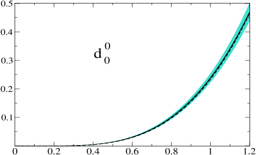
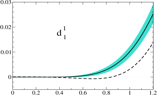
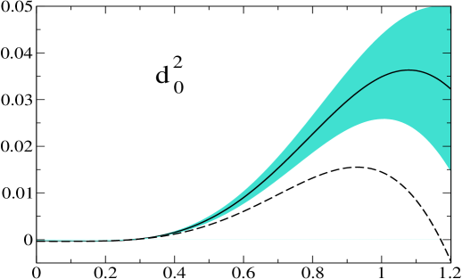
Figure 1: Driving terms versus energy in GeV. The full lines show the result of the calculation described in appendix B. The shaded regions indicate the uncertainties associated with the input of that calculation. The dashed curves represent the contributions from the $D$- and $F$-waves below 2 GeV.

As far as $d^{0}_{0}(s)$ is concerned, our result roughly agrees with earlier calculations [3, 6]. Our values for $d^{1}_{1}(s)$ and $d^{2}_{0}(s)$, however, are much smaller. The bulk of the difference is of purely kinematic origin: The values taken for $s_{2}$ are different. While we are working with $\sqrt{\rule[1.00006pt]{0.0pt}{5.0pt}s_{2}}=2\,\mbox{GeV}$, the values used in refs. [3] and [6] are $\sqrt{53}\,M_{\pi}\simeq 1\,\mbox{GeV}$ and $\sqrt{110}\,M_{\pi}\simeq 1.5\,\mbox{GeV}$, respectively. The value of $s_{2}$ enters the definition of the driving terms in eq. (3.2) as the lower limit of the integration over the imaginary parts of the $S$- and $P$-waves. We have checked that, once this difference in the range of integration is accounted for, the driving terms given in these references are consistent with the above representation. Note however, that our uncertainties are considerably smaller, and we do rely on this accuracy in the following. It then matters that not only the range of integration, but also the integrands used in [3, 6] differ from ours: In these references, it is assumed that, above the value taken for $s_{2}$, the behaviour of the $S$- and $P$-wave imaginary parts is adequately described by a Regge representation.

The difference between such a picture and our representation for the background amplitude is best illustrated with the simple model used in the early literature, where the asymptotic region is described by a Pomeron term with $\sigma_{tot}=20\,\mbox{mb}$ and a contribution from the $\rho\,$-$f$-trajectory, taken from the Lovelace-Shapiro-Veneziano model (appendix E). As discussed in detail in appendix B.4, the assumption that an asymptotic behaviour of this type sets in early is in conflict with crossing symmetry [43]. In particular, the model overestimates the contribution to the driving terms from the region above 1.5 GeV, roughly by a factor of two. Either the value of $\sigma_{tot}$ or the residue of the leading Regge trajectory or both must be reduced in order for the model not to violate the sum rule (B.6). The manner in which the asymptotic contribution is split into one from the Pomeron and one from the leading Regge trajectory is not crucial. For any reasonable partition that obeys the sum rule (B.6), the outcome for the driving terms is approximately the same. The result for $d^{1}_{1}(s)$ and $d^{2}_{0}(s)$ is considerably smaller than what is expected from the above model. The leading term $d^{0}_{0}(s)$, on the other hand, is dominated by the resonance $f_{2}(1275)$ and is therefore not sensitive to the behaviour of the imaginary parts in the region above $1.5\,\mbox{GeV}$.

5 Roy equations as integral equations

Once the driving terms are pinned down, the Roy equations for the $S$- and $P$- waves express the real parts of the partial waves in terms of the $S$-wave scattering lengths and of a principal value integral over their imaginary parts from $4M_{\pi}^{2}$ to $s_{2}$. Unitarity implies that, in the elastic domain $4M_{\pi}^{2}<s<16M_{\pi}^{2}$, the real and imaginary parts of the partial wave amplitudes are determined by a single real parameter, the phase shift. If we were to restrict ourselves to the elastic region, setting $s_{2}=16M_{\pi}^{2}$, the Roy equations would amount to a set of coupled, nonlinear singular integral equations for the phase shifts. We may extend this range, provided the elasticity parameters $\eta^{I}_{\ell}(s)$ are known. On the other hand, since the Roy equations do not constrain the behaviour of the partial waves for $s>68M_{\pi}^{2}$, the integrals occurring on the r.h.s. of these equations can be evaluated only if the imaginary parts in that region are known, together with the subtraction constants $a_{0}^{0}$, $a_{0}^{2}$, which also represent parameters to be assigned externally.

In the present paper, we do not solve the Roy equations in their full domain of validity, but use a smaller interval, $4M_{\pi}^{2}<s<s_{0}$. The reason why it is advantageous to use a value of $s_{0}$ below the mathematical upper limit, $s_{0}<s_{1}$, is that the Roy equations in general admit more than one solution. As will be discussed in detail in section 6, the solution does become unique if the value of $s_{0}$ is chosen between the $\rho$ mass and the energy where the $I=0$ $S$-wave phase passes through $\pi/2$ – this happens around $0.86$ GeV. In the following, we use

$$\sqrt{\rule[1.00006pt]{0.0pt}{5.0pt}s_{0}}=0.8\,\mbox{GeV}\;\;,\hskip 20.00003pts_{0}=32.9\,M_{\pi}^{2}\;\;.$$

In the variable $s$, our matching point is nearly at the center of the interval between threshold and $s_{1}=68\,M_{\pi}^{2}$. We are thus solving the Roy equations on the lower half of their range of validity, using the upper half to check the consistency of the solutions so obtained (section 10). Our results are not sensitive to the precise value taken for $s_{0}$ (section 9).

The Roy equations for the $S$- and $P$-waves may be rewritten in the form

$$\mbox{Re}\,t_{\ell}^{I}(s) \!\!\!\!= \!\!\!\!k_{\ell}^{I}(s)+-\int_{4M_{\pi}^{2}}^{s_{0}}ds^{\prime}K_{\ell\,0}^{I\,0}(s,s^{\prime})\,\mbox{Im}\,t_{0}^{0}(s^{\prime})+-\int_{4M_{\pi}^{2}}^{s_{0}}ds^{\prime}K_{\ell\,1}^{I\,1}(s,s^{\prime})\,\mbox{Im}\,t_{1}^{1}(s^{\prime})$$ (5.1)

$$\!\!\!\!+-\int_{4M_{\pi}^{2}}^{s_{0}}ds^{\prime}K_{\ell\,0}^{I\,2}(s,s^{\prime})\,\mbox{Im}\,t_{0}^{2}(s^{\prime})+f_{\ell}^{I}(s)+d_{\ell}^{I}(s)\;\;,$$

where $I$ and $\ell$ take only the values ($I,\ell$) =(0,0), (1,1) and (2,0). The bar across the integral sign denotes the principal value integral. The functions $f_{\ell}^{I}(s)$ contain the part of the dispersive integrals over the three lowest partial waves that comes from the region between $s_{0}$ and $s_{2}$, where we are using experimental data as input. They are defined as

$$f_{\ell}^{I}(s)=\sum_{I^{\prime}=0}^{2}\sum_{\ell^{\prime}=0}^{1}-\int_{s_{0}}^{s_{2}}ds^{\prime}K_{\ell\ell^{\prime}}^{II^{\prime}}(s,s^{\prime})\,\mbox{Im}\,t_{\ell^{\prime}}^{I^{\prime}}(s^{\prime})\;\;.$$ (5.2)

The experimental input used to evaluate these integrals will be discussed in section 7, together with the one for the elasticity parameters of the $S$- and $P$-waves.

One of the main tasks we are faced with is the construction of the numerical solution of the integral equations (5.1) in the interval $4M_{\pi}^{2}\leq s\leq s_{0}$, for a given input $\{a_{0}^{0},a_{0}^{2},f_{\ell}^{I},\eta_{\ell}^{I},d_{\ell}^{I}\}$. Once a solution is known, the real part of the amplitude can be calculated with these equations, also in the region $s_{0}\leq s\leq s_{1}$.

6 On the uniqueness of the solution

The literature concerning the mathematical structure of the Roy equations was reviewed in the introduction. In the following, we first discuss the situation for the single channel case – which is simpler, but clearly shows the salient features – and then describe the generalization to the three channel problem we are actually faced with. For a detailed analysis, we refer the reader to two recent papers on the subject [30, 31] and the references quoted therein.

6.1 Roy’s integral equation in the one-channel case

If we keep only the diagonal, singular Cauchy kernel in (1.1), the partial wave relations decouple, and the left hand cut in the amplitudes disappears. Each one of the three partial wave amplitudes then obeys the following conditions:

i) In the interval between the threshold $s=4M_{\pi}^{2}$ and the matching point $s=s_{0}$, the real part is given by a dispersion relation

$${\rm Re}\,t(s)=a+(s-4M_{\pi}^{2})\,{1\over\pi}-\int_{4M_{\pi}^{2}}^{\infty}ds^{\prime}\,{{\rm Im}\,t(s^{\prime})\over(s^{\prime}-4M_{\pi}^{2})\,(s^{\prime}-s)}\;.$$ (6.1)

ii) Above $s_{0}$, the imaginary part ${\rm Im}\,t(s)$ is a given input function

$${\rm Im}\,t(s)=A(s),\qquad s\geq s_{0}\;.$$ (6.2)

iii) For simplicity, we take the matching point in the elastic region, so that

$$t(s)=\frac{1}{\sigma(s)}e^{i\delta(s)}\sin{\delta(s)}\;\;,\hskip 20.00003pt4M_{\pi}^{2}\leq s\leq s_{0}\;\;,$$ (6.3)

where $\delta(s)$ is real and vanishes at threshold. We refer the reader to [30] for a precise formulation of the regularity properties required from the amplitude and from the input absorptive part. As a minimal condition, we must require

$$\lim_{s\nearrow s_{0}}\,{\rm Im}\,\,t(s)=A(s_{0})\;\;.$$ (6.4)

Otherwise, the principal value integral does not exist at the matching point.

Equations (6.1)–(6.4) constitute the mathematical problem we are faced with in this case: Determine the amplitudes $t(s)$ that verify these equations for a given input of scattering length $a$ and absorptive part $A(s)$. Once a solution is known, the real part of the amplitude above $s_{0}$ is obtained from the dispersion relation (6.1), and $t(s)$ is then defined on $4M_{\pi}^{2}\leq s<\infty$. The following points summarize the results relevant in our context:

1. Elastic unitarity reduces the problem to the determination of the real function $\delta(s)$, defined in the interval $4M_{\pi}^{2}\leq s\leq s_{0}$. The amplitude $t(s)$ is then obtained from (6.3).

2. A given input $\{a,A(s)\}$ does not, in general, fix the solution uniquely – in addition, the value of the phase at the matching point plays an important role. Indeed, let $t(s)$ be a solution and suppose first that the phase at the matching point is positive. For $0<\delta(s_{0})<\pi/2$, the infinitesimal neighbourhood of $t(s)$ does not contain further solutions. For $\delta(s_{0})>\pi/2$, however, the neighbourhood contains an $m$-parameter family of solutions. The integer $m$ is determined by the value of the phase at the matching point ($\left[x\right]$ is the largest integer not exceeding $x$):

   $$m=\left[2\delta(s_{0})\over\pi\right]\;\;.$$ (6.5)

   For a monotonically increasing phase, the index $m$ counts the number of times $\delta(s)$ goes through multiples of $\pi/2$ as $s$ varies from threshold to the matching point. We illustrate the situation for $m=0,1,2$ in figure 2.

   a) $m=0$	b) $m=1$	c) $m=2$

   Figure 2: Boundary conditions on the phase $\delta(s_{0})$ for solving Roy’s integral equation. Figs. a,b,c represent the cases $0<\delta(s_{0})<\pi/2$, $\pi/2<\delta(s_{0})<\pi$ and $\pi<\delta(s_{0})<3\pi/2$, respectively. In fig. c, the phase winds around the Argand circle slightly more than once.

3. If the value of the phase at the matching point is negative, the problem does not in general have a solution. In order for the problem to be soluble at all, the input must be tuned. For $-\pi/2<\delta(s_{0})<0$, for instance, we may keep the absorptive part $A(s)$ as it is, but tune the scattering length $a$. This situation may be characterized by $m=-1$: Instead of having a family of solutions containing free parameters, the input is subject to a constraint. Once a solution does exist, it is unique in the sense that the infinitesimal neighbourhood does not contain further solutions.

4. Consider now the case displayed in fig. 2a, where the phase at the matching point is below $\pi/2$. This corresponds to the situation encountered in the coupled channel case, for our choice of the matching point. According to the above statements, a given input $\{a,A(s)\}$ then generates a locally unique solution – if a solution exists at all. We take it that uniqueness also holds globally, see [15].

The solution may be constructed in the following manner: Consider a family of unitary amplitudes, parametrized through $c_{1},\ldots,c_{n}$. For any given amplitude, evaluate the right and left hand sides of eq. (6.1) and calculate the square of the difference at $N$ points in the interval $4M_{\pi}^{2}\leq s\leq s_{0}$. Finally, minimize the sum of these squares by choosing $c_{1},\dots,c_{n}$ accordingly. Since the solution is unique, it suffices to find one with this method – it is then the only one.

6.2 Cusps

In general, the solutions are not regular at the matching point, but have a cusp (branch point) there: $\delta(s)=\delta(s_{0})+C(s_{0}-s)^{\gamma}+\ldots\,$, with $\gamma>0$. The phenomenon arises from our formulation of the problem – the physical amplitude is regular there. We conclude that, even if a mathematical solution can be constructed for a given input $\{a,A(s)\}$, it will in general not be acceptable physically, because it contains a fictitious singularity at the matching point. The behaviour of the phase is sensitive to the value of the exponent: If $\gamma$ is close to 1, the discontinuity in the derivative is barely visible, while for small values of $\gamma$, it manifests itself very clearly.

The strength of the singularity is determined by the constant $C$, whose value depends on the input used. In particular, if the scattering length $a$ is varied, while the absorptive part $A(s)$ is kept fixed, the size of $C$ changes. We may search for the value of $a$ at which $C$ vanishes. Although the singularity does not disappear entirely even then, it now only manifests itself in the derivatives of the function (for the solution to become analytic at $s_{0}$, we would need to also adapt the input for $A(s)$). In view of the fact that our solutions are inherently fuzzy, because the values of the input are subject to experimental uncertainties, we consider solutions with $C\simeq 0$ or $\gamma\simeq 1$ as physically acceptable and refer to these as solutions without cusp.

The search for solutions without cusp can be implemented as follows. Instead of fixing $a$, constructing solutions in the class of functions with a cusp and then determining the value of $a$ at which the cusp disappears, we may simply consider parametrizations that do not contain a cusp, treating the scattering length $a$ as a free parameter, on the same footing as the set $c_{1},\ldots,c_{n}$ used to parametrize the phase shift and minimizing the difference between the left and right hand sides of eq. (6.1). We have verified that if a solution without cusp does exist, this procedure indeed finds it: Allowing for the presence of cusps does not lead to a better minimum.

The net result of this discussion is that the scattering length $a$ must match the input for $A(s)$ – it does not represent an independent parameter. When solving the Roy equations, we can at the same time also determine the value of $a$ that belongs to a given input for the high energy absorptive part. The conclusion remains valid even if the matching point is above the first inelastic threshold, provided the elasticity parameter $\eta$ is known and sufficiently smooth at the matching point. For a thorough analysis of the issue, we refer to [31].

6.3 Uniqueness in the multi-channel case

In the multichannel case, we need to determine three functions $\delta_{0}^{0},\delta_{1}^{1}$ and $\delta_{0}^{2}$ for a given input $\{a_{0}^{0},a_{0}^{2},f_{\ell}^{I},\eta_{\ell}^{I},d_{\ell}^{I}\}$. The multiplicity index $m$ of the infinitesimal neighbourhood of a given solution is displayed in table 1 [31], for various values of the matching point $s_{0}$. The table contains the following information. In the situations indicated with the labels I and II, the infinitesimal neighbourhood of a given solution contains a family of solutions, characterized by 2 and 1 free parameters, respectively. In case III, the solution is unique in the sense that the neighbourhood does not contain further solutions, while in case IV a solution only exists if the input is subject to a constraint ($m=-1$, compare paragraph 3 in section 6.1). In order to uniquely characterize the solution in case I, for instance, we thus need to fix two more parameters – in addition to the input – say the position of the $\rho$ resonance and its width, or the position of the $\rho$ resonance and the value of $s$ where the $I=0$ phase passes through $\pi/2$, and similarly for II. In the following, we stick to case III, where the solution is unique for a given input. As discussed above, each of the three partial waves will in general develop a cusp at the matching point $s_{0}$, unless some of the input parameters take special values.

	range of $s_{0}$	range of $\delta_{0}^{0}$	range of $\delta_{1}^{1}$	$m$
I	$\rule{0.0pt}{13.00005pt}\rule{18.00005pt}{0.0pt}1<\sqrt{\rule[1.00006pt]{0.0pt}{5.0pt}s_{0}}<1.15$	$\rule{6.99997pt}{0.0pt}\pi<\delta_{0}^{0}<\frac{3}{2}\,\pi$	$\frac{1}{2}\,\pi<\delta_{1}^{1}<\pi$	2
II	$\rule{5.0pt}{0.0pt}0.86<\sqrt{\rule[1.00006pt]{0.0pt}{5.0pt}s_{0}}<1$	$\frac{1}{2}\,\pi<\delta_{0}^{0}<\pi$	$\frac{1}{2}\,\pi<\delta_{1}^{1}<\pi$	1
III	$\rule{5.0pt}{0.0pt}0.78<\sqrt{\rule[1.00006pt]{0.0pt}{5.0pt}s_{0}}<0.86$	$\rule{8.00003pt}{0.0pt}0<\delta_{0}^{0}<\frac{1}{2}\,\pi$	$\frac{1}{2}\,\pi<\delta_{1}^{1}<\pi$	0
IV	$\rule{5.0pt}{0.0pt}0.28<\sqrt{\rule[1.00006pt]{0.0pt}{5.0pt}s_{0}}<0.78$	$\rule{8.00003pt}{0.0pt}0<\delta_{0}^{0}<\frac{1}{2}\,\pi$	$\rule{8.99994pt}{0.0pt}0<\delta_{1}^{1}<\frac{1}{2}\,\pi$	$-1$

Table 1: Multiplicity of solutions in the coupled channel case. The multiplicity index $m$ is the number of free parameters occurring in the solutions of the Roy equations, if the matching point $s_{0}$ is in the interval indicated (in GeV units). Also displayed is the variation of the physical phases $\delta_{0}^{0}$ and $\delta_{1}^{1}$ on that interval.

The situation encountered in practice is the following. Let $0.1<a_{0}^{0}<0.6$, and let $f_{\ell}^{I}$, $\eta^{I}_{\ell}$ and $d_{\ell}^{I}$ be fixed as well. For an arbitrary value of the scattering length $a_{0}^{2}$, the solution in general develops a strong cusp in the $P$-wave. This cusp can be removed by tuning $a_{0}^{2}\rightarrow\bar{a}_{0}^{2}$, using for instance the method described in the single channel case above. Remarkably, it turns out that the solutions so obtained are nearly free of cusps in the two $S$-waves as well. The problem manifests itself almost exclusively in the $P$-wave, because our matching point is rather close to the mass of the $\rho$, where the imaginary part shows a pronounced peak. If $a_{0}^{2}$ is chosen to slightly differ from the optimal value $\bar{a}_{0}^{2}$, a cusp in the $P$-wave is clearly seen. We thus obtain a relation between the scattering lengths $a_{0}^{0}$ and $a_{0}^{2}$. This is how the so-called universal curve, discovered a long time ago [44], shows up in our framework. We will discuss the properties of this curve in detail below.

In principle, we might try to also fix $a_{0}^{0}$ with this method, requiring that there be no cusp in one of the two $S$-waves. The cusps in these are very weak, however – the procedure does not allow us to accurately pin down the second scattering length. The choice $a_{0}^{0}=-0.2$, for instance, still leads to a fully acceptable solution. On the other hand, we did not find a solution in the class of smooth functions for $a_{0}^{0}=-0.5$. This shows that the analyticity properties that are not encoded in the Roy integral equations (5.1) do constrain the range of admissible values for $a_{0}^{0}$, but since that range is very large, the constraint is not of immediate interest, and we do not consider the matter further. In our numerical work, we consider values in the range $0.15<a_{0}^{0}<0.30$ and use the center of this interval, $a_{0}^{0}=0.225$, as our reference point.

7 Experimental input

In this section, we describe the experimental input used for the elasticity below the matching point at $\sqrt{\rule[1.00006pt]{0.0pt}{5.0pt}s_{0}}=0.8\,\mbox{GeV}$ and for the imaginary parts of the $S$- and $P$-waves in the energy interval between $\sqrt{\rule[1.00006pt]{0.0pt}{5.0pt}s_{0}}$ and $\sqrt{\rule[1.00006pt]{0.0pt}{5.0pt}s_{2}}=2\,\mbox{GeV}$. The references are listed in [45]–[59] and for an overview, we refer to [9, 60]. The evaluation of the contributions from the higher partial waves and from the asymptotic region ($s>s_{2}$) is discussed in detail in appendix B.

7.1 Elasticity below the matching point

The Roy equations allow us to determine the phase shifts of the $S$- and $P$-waves only if – on the interval between threshold and the matching point – the corresponding elasticity parameters $\eta_{0}^{0}(s)$, $\eta_{1}^{1}(s)$ and $\eta_{0}^{2}(s)$ are known. On kinematic grounds, the transition $2\pi\rightarrow 4\pi$ is the only inelastic channel open below our matching point, $\sqrt{\rule[1.00006pt]{0.0pt}{5.0pt}s_{0}}=0.8\,\mbox{GeV}$. The threshold for this reaction is at $E=4\,M_{\pi}\simeq 0.56\,\mbox{GeV}$, but phase space strongly suppresses the transition at low energies – a significant inelasticity only sets in above the matching point. In particular, the transition $\pi\pi\rightarrow K\bar{K}$, which occurs for $E>2\,M_{K}\simeq 0.99\,\mbox{GeV}$, does generate a well-known, pronounced structure in the elasticity parameters of the waves with $I=0,1$. Below the matching point, however, we may neglect the inelastic reactions altogether and set

$$\eta^{0}_{0}(s)=\eta^{1}_{1}(s)=\eta^{2}_{0}(s)=1\;\;,\hskip 20.00003pt\sqrt{s}<0.8\,\mbox{GeV}\;\;.$$

We add a remark concerning the effects generated by the inelastic reaction $2\pi\rightarrow 4\pi$, which are analyzed in ref. [57]. In one of the phase shift analyses given there (solution A), the inelasticity $1-\eta_{1}^{1}(s)$ reaches values of order 4%, already in the region of the $\rho\,$-resonance. The effect is unphysical – it arises because the parametrization used does not account for the strong phase space suppression at the $4\pi$ threshold. For the purpose of the analysis performed in ref. [57], which focuses on the region above 1 GeV, this is immaterial, but in our context, it matters: We have solved the Roy equations also with that representation for the elasticities. The result shows significant distortions, in particular in the $P$-wave.

7.2 Input for the $I=0,1$ channels

The experimental information on the $\pi\pi$ phase shifts in the intermediate energy region comes mainly from the reaction $\pi N\rightarrow\pi\pi N$. A rather involved analysis is necessary to extract the $\pi\pi$ phase shifts from the raw data, and several different representations for the phases and elasticities are available in the literature. The main source of experimental information is still the old measurement of the reaction $\pi^{-}p\rightarrow\pi^{-}\pi^{+}n$ by the CERN–Munich (CM) collaboration [49], but there are also older, statistically less

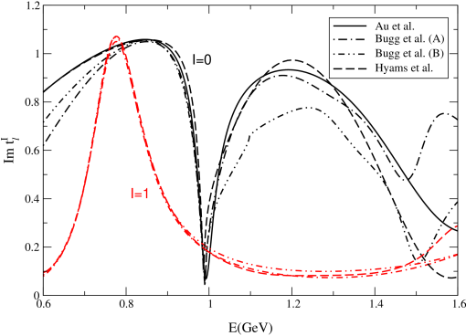
Figure 3: Comparison of the different input we used for the imaginary parts of the $I=0$ and $I=1$ lowest partial waves above the matching point at 0.8 GeV.

precise data, for instance from Saclay [45] and Berkeley [48], as well as newer ones, such as the data of the CERN-Cracow-Munich collaboration concerning pion production on polarized protons [54] and those on the reaction $\pi^{-}p\rightarrow\pi^{0}\pi^{0}n$, obtained recently by the E852 collaboration at Brookhaven [59]. For a detailed discussion of the available experimental information, we refer to [9, 57, 60].

For our purposes, energy-dependent analyses are most convenient, because these yield analytic expressions for the imaginary parts, so that the relevant integrals can readily be worked out. To illustrate the differences between these analyses, we plot the corresponding imaginary parts in fig. 3, both for the $I=0$ $S$-wave and for the $P$-wave. The representations of refs. [47, 55, 57] do not extend to 2 GeV, but they do cover the range between 0.8 and 1.7 GeV. Unitarity ensures that the contributions generated by the imaginary parts of the $S$- and $P$-waves in the region between 1.7 and 2 GeV are very small, so that we may use these representations also there without introducing a significant error. For the $P$-wave, the differences between the various parametrizations are not dramatic, but for the $I=0$ $S$-wave, they are quite substantial. Despite these differences, the result obtained for the dispersive integrals are similar, at least in the range where we are solving the Roy equations. This can be seen in fig. 4, where we plot the value of the dispersion integral $f^{0}_{0}$, defined in eq. (5.2). The only visible difference is between parametrization B of ref. [57] and the others. In order of magnitude, the effect is comparable to the one occurring if the scattering length $a^{0}_{0}$ is shifted by $0.01$.

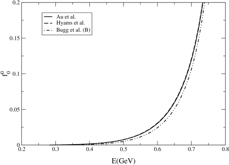
Figure 4: Comparison of the results obtained for the dispersion integral $f^{0}_{0}$ with the various imaginary parts shown in fig. 3.

It arises from the difference in the behaviour of the $S$-wave imaginary part in the region between 1 and 1.5 GeV. The phase shift analysis of Protopopescu et al. [48] does not cover that region, as it only extends to 1.15 GeV, but those of Au, Morgan and Pennington [55] as well as Bugg, Sarantsev and Zou [57] do. Both of these include, aside from the CM data, additional experimental information, not included in the analysis of Hyams et al. [47].

In the following, we rely on the representation of Au et al. [55] for the $S$-wave and the one of Hyams et al. [47] for the $P$-wave (the analysis of Au et al. does not include the $P$-wave). We have verified that, using [47] also for the $S$-wave would not change our results below the matching point, beyond the uncertainties to be attached to the solutions, anyway. On the other hand, Au et al. [55] yield a more consistent picture above the matching point – for this reason we stick to that analysis. More precisely, we use the solution denoted by $K_{1}$(Etkin) in ref. [55], table I. That solution contains a narrow resonance in the 1 GeV region, which does not occur in the other phase shift analyses. In our opinion, the extra state is an artefact of the representation used: A close look reveals that the occurrence of this state hinges on small details of the $K$-matrix representation. In fact, the resonance disappears if two of the $K$-matrix coefficients are slightly modified, for instance with $(-c_{12}^{0},-c_{22}^{0})=(3.1401,2.8447)\rightarrow(3.2019,2.6023)$.

7.3 Phase of the $P$-wave from $e^{+}e^{-}\rightarrow\pi^{+}\pi^{-}$ and $\tau\rightarrow\pi^{-}\pi^{0}\,\nu_{\tau}$

For the $P$-wave, the data on the processes $e^{+}e^{-}\rightarrow\pi^{+}\pi^{-}$ and $\tau\rightarrow\pi^{-}\pi^{0}\,\nu_{\tau}$ yield very useful, independent information. The corresponding transition amplitude is proportional to the pion form factor $F_{\scriptscriptstyle e.m.}(s)$ of the electromagnetic current and to the form factor $F_{\scriptscriptstyle V}(s)$ of the charged vector current, respectively. The data provide a measurement of the quantities $|F_{\scriptscriptstyle e.m.}(s)|$ and $|F_{\scriptscriptstyle V}(s)|$ in the time-like region, $s>4M_{\pi}^{2}$.

In the isospin limit, the two form factors coincide: The currents only differ by an isoscalar operator that carries odd $G$-parity, so that the pion matrix elements thereof vanish. While the isospin breaking effects in $|F_{\scriptscriptstyle V}(s)|$ are very small, $\rho-\omega$ interference does produce a pronounced structure in the electromagnetic form factor. The $\omega$-resonance generates a second sheet pole in the isoscalar matrix elements, at $s=(M_{\omega}-i\,\frac{1}{2}\,\Gamma_{\omega})^{2}$. The residue of the pole is small, of order $O(m_{d}-m_{u},e^{2})$, but in view of the small width of the $\omega$, the denominator also nearly vanishes for $s=M_{\omega}^{2}$. Moreover, the pole associated with the exchange of a $\rho$ occurs in the immediate vicinity of this point, so that the transition amplitude involves a sum of two contributions that rapidly change with $s$, both in magnitude and phase. Since the interference phenomenon is well understood, it can be corrected for. When this is done, the data on the two processes $e^{+}e^{-}\rightarrow\pi^{+}\pi^{-}$ and $\tau\rightarrow\pi^{-}\pi^{0}\nu$ are in remarkably good agreement (for a review, see [61, 62]).

We denote the phase of the vector form factor by $\phi(s)$,

$$F_{\scriptscriptstyle V}(s)=|F_{\scriptscriptstyle V}(s)|\,e^{\,i\,\phi(s)}\;\;.$$

In the elastic region $4M_{\pi}^{2}<s<16M_{\pi}^{2}$, the final state interaction exclusively involves $\pi\pi$ scattering, so that the Watson theorem implies that the phase $\phi(s)$ coincides with the $P$-wave phase shift,

$$\phi(s)=\delta_{1}^{1}(s)\;\;,\hskip 20.00003pt4M_{\pi}^{2}<s<16M_{\pi}^{2}\;\;.$$

In fact, phase space suppresses the inelastic channels also in this case – the available data on the decay channel $\tau\rightarrow 4\,\pi\,\nu_{\tau}$ show that, for $E<0.9\,\mbox{GeV}$, the inelasticity is below 1%, so that the phase of the form factor must agree with the $P$-wave phase shift, to high accuracy [63].

In the region where the singularity generated by $\rho\,$-exchange dominates, in particular also in the vicinity of our matching point, the form factor is well represented by a resonance term and a slowly varying background. Quite a few such representations may be found in the recent literature. Since the uncertainties in the data (statistical as well as systematic) are small, these parametrizations agree quite well. In the following, we use the Gounaris-Sakurai representation of ref. [64] as a reference point. That representation involves a linear superposition of three resonance terms, associated with $\rho(770)$, $\rho(1450)$ and $\rho(1700)$. We have investigated the uncertainties to be attached to this representation by (a) comparing the magnitude of the form factor with the available data, (b) comparing it with other parametrizations, (c) varying the resonance parameters in the range quoted in ref. [64] and (d) using the fact that analyticity imposes a strong correlation between the phase of the form factor and its magnitude. On the basis of this analysis, we conclude that the $e^{+}e^{-}$ and $\tau$ data determine the phase of the $P$-wave at $0.8\,\mbox{GeV}$ to within an uncertainty of $\pm 2^{\circ}$. A detailed comparison between the phase of the form factor and the solution of the Roy equations for the $P$-wave will be given in section 12.2.

7.4 Phases at the matching point

In the framework of our analysis, the input used for $s\geq s_{0}$ enters in two ways: (i) it specifies the value of the three phases at the matching point and (ii) it determines the contributions to the Roy equation integrals from the region above that point. Qualitatively, we are dealing with a boundary value problem: At threshold, the phases vanish, while at the matching point, they are specified by the input. The solution of the Roy equations then yields the proper interpolation between these boundary values. The behaviour of the imaginary parts above the matching point is less important than the boundary values, because it only affects the slope and the curvature of the solution.

$\rule{16.99998pt}{0.0pt}\delta_{0}^{0}$	$\rule{16.99998pt}{0.0pt}\delta_{1}^{1}$	$\rule{5.0pt}{0.0pt}\delta_{1}^{1}-\delta_{0}^{0}\rule{20.00003pt}{0.0pt}$	reference
81.7 $\pm$ 3.9	105.2 $\pm$ 1.0	23.4 $\pm$ 4.0	[46, 47]
90.4 $\pm$ 3.6	115.2 $\pm$ 1.2	24.8 $\pm$ 3.8	[50] s-channel moments
85.7 $\pm$ 2.9	116.0 $\pm$ 1.8	30.3 $\pm$ 3.4	[50] t-channel moments
81.6 $\pm$ 4.0	108.1 $\pm$ 1.4	26.5 $\pm$ 4.2	[48] table VI
80.9	105.9	25.0	[46, 47]
79.5	106.1	26.5	[57] solution A
79.9	106.8	26.9	[57] solution B
80.7	$\rule{10.00002pt}{0.0pt}-$	$\rule{5.0pt}{0.0pt}-$	[55] solution K1
82.0	$\rule{10.00002pt}{0.0pt}-$	$\rule{5.0pt}{0.0pt}-$	[55] solution K1(Etkin)

Table 2: Value of the phases $\delta_{0}^{0}$ and $\delta_{1}^{1}$ at 0.8 GeV. The first three rows stem from analyses of the data at a fixed value of the energy (“energy independent”), while the remaining entries are obtained from a fit to the data that relies on an explicit parametrization of the energy dependence (“energy dependent analysis”).

We now discuss the available information for the phases $\delta_{0}^{0}$ and $\delta_{1}^{1}$ at the matching point. The values obtained from the high energy, high statistics $\pi N\rightarrow\pi\pi N$ experiments are collected in table 2. In those cases where the published numbers do not directly apply at $0.8\,\mbox{GeV}$, we have used a quadratic interpolation between the three values of the energy closest to this one. The errors given in the third column are obtained by adding those from the first two columns in quadrature. For the energy dependent entries, the error analysis is more involved – only ref. [48] explicitly quotes an error. The scatter seen in the table partly arises from the fact that different methods of analysis are used. The corresponding systematic uncertainties are not covered by the error bars quoted in the individual phase shift analyses: Taken at face value, the numbers listed in the table are contradictory, particularly in the case of the $P$-wave. For a thorough discussion of the experimental discrepancies, we refer to [60].

As discussed above, both the statistical and the systematic uncertainties of the $e^{+}e^{-}$ and $\tau$ data are considerably smaller. They constrain the phase of the $P$-wave at 0.8 GeV to a narrow range, centered around the value $\delta_{1}^{1}(s_{0})=108.9^{\circ}$ obtained with the Gounaris-Sakurai representation of the form factor in ref. [64]:

$$\delta_{1}^{1}(s_{0})=108.9^{\circ}\pm 2^{\circ}\;\;.$$ (7.1)

The comparison with the numbers listed in the second column of the table shows that this value is within the range of the results obtained from $\pi N\rightarrow\pi\pi N$.

Unfortunately, the $e^{+}e^{-}$ and $\tau$ data only concern the $P$-wave. To pin down the $I=0$ $S$-wave, we observe that the overall phase of the scattering amplitude drops out when considering the difference $\delta_{1}^{1}-\delta_{0}^{0}$, so that one of the sources of systematic error is absent. Indeed, the third column in the table shows that the outcome of the various analyses is consistent with the assumption that the fluctuations seen are of statistical origin. The statistical average of the energy independent analyses yields $\delta_{1}^{1}(s_{0})-\delta_{0}^{0}(s_{0})=26.6^{\circ}\pm 3.7^{\circ}$, with $\chi^{2}=2$ for 2 degrees of freedom (as the numbers are based on the same data, we have inflated the error bar – the number given is the mean error of the three data points). The remaining entries in the table neatly confirm this result. Combining it with the one in the fourth row, which is based on independent data, we finally arrive at

$$\delta_{1}^{1}(s_{0})-\delta_{0}^{0}(s_{0})=26.6^{\circ}\pm 2.8^{\circ}\;\;.$$ (7.2)

Since the value for $\delta_{1}^{1}$ comes from the data on the form factor, while the one for the difference $\delta_{1}^{1}-\delta^{0}_{0}$ is based on the reaction $\pi N\rightarrow\pi\pi N$, these numbers are independent, so that it is legitimate to combine them. Adding errors quadratically, we obtain

$$\delta^{0}_{0}(s_{0})=82.3^{\circ}\pm 3.4^{\circ}\;\;.$$ (7.3)

In the following, we rely on the two values for the phases at the matching point given in eqs. (7.1) and (7.3). We emphasize that the $\pi N\rightarrow\pi\pi N$ data are consistent with these – in fact, the result of the energy-dependent analysis quoted in the fourth row of the table is in nearly perfect agreement with the above numbers. We are exploiting the fact that the $e^{+}e^{-}$ and $\tau$ data strongly constrain the behaviour of the $P$-wave in the region of the $\rho$, thus reducing the uncertainties in the value of $\delta_{1}^{1}$ at the matching point.

For the principal value integrals to exist, we need to continuously connect the values of the imaginary parts calculated from the phases at the matching point with those of the phase shift representation we wish to use. This can be done, either by slightly modifying the parameters occurring in the representation in question or with a suitable interpolation of the phases between the matching point and $K\bar{K}$ threshold. We have checked that our results do not depend on how that is done, as long as the interpolation is smooth. Note that, for the representation $K_{1}$(Etkin) [55] – our reference input for the imaginary part of the $I=0$ $S$-wave – an interpolation is not needed: The last row of table 2 shows that, at the matching point, this representation nearly coincides with the central value in eq. (7.3).

7.5 Input for the $I=2$ channel

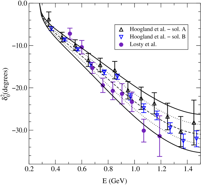
Figure 5: Different data sets for the $S$-wave in the $I=2$ channel and curves that we have used as input in the Roy equation analysis.

The uncertainties in this channel are rather large. The current experimental situation is summarized in fig. 5, where we show the data points from the two main experiments [51, 53], and five different parametrizations that we will use as input. The central one is our best fit to the data of the Amsterdam–CERN–Munich collaboration (ACM) [53] solution B (which we call from now on ACM(B)) with a parametrization à la Schenk [65]. To cover the rather wide scatter of the data, we have varied the input in this channel, using the five curves shown in the figure, together with $\eta^{2}_{0}=1$ (note that for the Roy equation analysis, only the value of the scattering length $a^{2}_{0}$ and the behaviour of the imaginary part above 0.8 GeV matter).

8 Numerical solutions

In the preceding section, the input required to evaluate the r.h.s. of our system of equations was discussed in detail. In the present section, we describe the numerical method used to solve this system and illustrate the outcome with an example.

8.1 Method used to find solutions

We search for solutions of the Roy equations by numerically minimizing the square of the difference between the left and right hand sides of eq. (5.1) in the region between threshold and 0.8 GeV. As we are neglecting the inelasticity in this region, the real and imaginary parts of $t^{I}_{\ell}(s)$ are determined by a single real function, the phase $\delta_{\ell}^{I}(s)$. In principle, the minimization should be performed over the whole space of physically acceptable functions $\{\delta_{0}^{0}(s),\;\delta_{1}^{1}(s),\;\delta_{0}^{2}(s)\}$, but for obvious practical reasons we restrict ourselves to functions described by a simple parametrization. We will use the one proposed by Schenk some time ago [65], allowing for an additional parameter in the polynomial part:

$$\tan\delta_{\ell}^{I}=\sqrt{1-{4M_{\pi}^{2}\over s}}\;q^{2\ell}\left\{A^{I}_{\ell}+B^{I}_{\ell}q^{2}+C^{I}_{\ell}q^{4}+D^{I}_{\ell}q^{6}\right\}\left({4M_{\pi}^{2}-s^{I}_{\ell}\over s-s^{I}_{\ell}}\right)\;\;,$$ (8.1)

The first term represents the scattering length, while the second is related to the effective range:

$$a^{I}_{\ell}=A^{I}_{\ell}\;\;,\hskip 20.00003ptb^{I}_{\ell}=B_{\ell}^{I}+{4\over s^{I}_{\ell}-4M^{2}_{\pi}}\,A_{\ell}^{I}-\frac{1}{M_{\pi}^{2}}\,\left(A^{I}_{\ell}\right)^{3}\delta_{\ell\,0}\;\;.$$ (8.2)

In each channel, one of the five parameters is fixed in order to ensure the proper value of the phase at $s_{0}$. Moreover the $S$-wave scattering lengths $a^{0}_{0}$ and $a^{2}_{0}$ are identified with the two constants that specify the subtraction polynomials in the Roy equations. As discussed in sect. 6, we need to tune the value of $a_{0}^{2}$ in order to avoid cusps. Treating this parameter on the same footing as the others, we are dealing altogether with $15-3-1=11$ free variables, to be determined by a minimization procedure. Our choice of $s_{0}$ ensures that the solution is unique, and therefore the method is safe: The choice of a bad parametrization would manifest itself in a failure of the minimization method – the minimum would not yield a decent solution.

The square of the difference between the left and right hand sides of the Roy equations is calculated at 22 points between threshold and $s_{0}$ for each of the three waves, so that the sum of squares ($\Delta_{\mbox{\tiny{Roy}}}^{2}$) contains 66 terms. The minimization of the function ($\Delta_{\mbox{\tiny{Roy}}}^{2}$) over $11$ parameters can be handled by standard numerical routines [66]. Our procedure does generate decent solutions: The differences between the left and right hand sides of the Roy equations are not visible on our plots – they are typically of order $10^{-3}$. The equations could be solved even more accurately by allowing for more degrees of freedom in the parametrization of the phases, but, in view of the uncertainties in the input, the accuracy reached is perfectly sufficient. Note also that the exact solution corresponding to a given input contains cusps. We have checked that these are too small to matter: Enlarging the space of functions on which the minimum is searched by explicitly allowing for such cusps in the parametrization of the phases, we find that the solutions remain practically the same.

8.2 Illustration of the solutions

To illustrate various features of our numerical solutions, we freeze for a moment all the inputs and analyze the properties of the specific solution we then get. The input for the imaginary parts above $s_{0}$ is the following: For the $I=0$ wave, we use the parametrization labelled $K_{1}$ (Etkin) of Au et al. [55]. In the case of the $I=1$ wave, we rely on the energy–dependent analysis of Hyams et al. [47], smoothly modified between $s_{0}$ and $4M_{K}^{2}$ to match the value $\delta_{1}^{1}(s_{0})=108.9^{\circ}$. For the $I=2$ wave, we take the central curve in fig. 5. The driving terms are specified in eq. (4). Moreover we fix $a_{0}^{0}=0.225$.

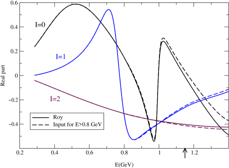
Figure 6: Numerical solution of the Roy equations for $a_{0}^{0}=0.225$, $a_{0}^{2}=-0.0371$ (the value of $a_{0}^{0}$ corresponds to the center of the range considered while the one of $a_{0}^{2}$ results if the input used for $\mbox{Im}\,t^{2}_{0}$ is taken from the central curve in fig. 5). The arrow indicates the limit of validity of the Roy equations.

With this input, the minimization leads to $a^{2}_{0}=-0.0371$ and the Schenk parameters take the values listed in table 3, in units of $M_{\pi}$.

	$I=0\rule{15.00002pt}{0.0pt}$	$I=1\rule{15.00002pt}{0.0pt}$	$I=2\rule{15.00002pt}{0.0pt}$
$A^{I}_{\ell}$	$\rule{0.0pt}{11.99998pt}0.225\rule{16.00008pt}{0.0pt}$	$3.63\cdot 10^{-2}$	$-3.71\cdot 10^{-2}$
$B^{I}_{\ell}$	$0.246\rule{16.00008pt}{0.0pt}$	$1.34\cdot 10^{-4}$	$-8.55\cdot 10^{-2}$
$C_{\ell}^{I}$	$-1.67\cdot 10^{-2}$	$-6.98\cdot 10^{-5}$	$-7.54\cdot 10^{-3}$
$D_{\ell}^{I}$	$-6.40\cdot 10^{-4}$	$1.41\cdot 10^{-6}$	$1.99\cdot 10^{-4}$
$\rule{1.99997pt}{0.0pt}s_{\ell}^{I}$	$36.7\rule{18.00005pt}{0.0pt}$	$30.7\rule{18.00005pt}{0.0pt}$	$-11.9\rule{18.00005pt}{0.0pt}$

Table 3: Schenk parameters of the solution shown in fig. 6.

The plot in fig. 6 shows that the numerical solution is indeed very good: Below $s_{0}$, it is not possible to distinguish the two curves representing the right and left hand sides of eq. (5.1). For this solution we found as a minimum $\Delta_{\mbox{\tiny{Roy}}}^{2}=2.1\cdot 10^{-5}$, which corresponds to an average difference between the right and left hand sides of about $6\cdot 10^{-4}$.

Having solved the Roy equations in the low–energy region, we now have a representation for the imaginary parts of the three lowest partial waves from threshold up to $s_{2}$. Since the driving terms account for all remaining contributions, we can then calculate the Roy representation for the real parts from threshold up to 1.15 GeV (full lines in fig.6). On the same plot, above $s_{0}$, we also show the real part of the partial wave representation that we used as an input for the imaginary parts (dashed lines). The comparison shows that the input we are using is well compatible with the Roy equations (we should stress at this point that in none of the phase–shift analyses which we are using as input the Roy equations have been used).

9 Universal band

As we have discussed in the preceding sections, for a given value of $a_{0}^{0}$ and fixed input, the Roy equations admit a solution without cusp only for a single value of $a_{0}^{2}$. By varying the input value of $a_{0}^{0}$, the Roy equations define a function $a_{0}^{2}=F(a_{0}^{0})$ that is known in the literature as the “universal curve” [44]. The experimental uncertainties in the input above 0.8 GeV convert this curve into a band. The universal band is the area in the $(a_{0}^{0},a_{0}^{2})$ plane that is allowed by the constraints given by the $\pi\pi$–scattering data above 0.8 GeV and the Roy equations. In this section we give a more precise definition of our universal band, and calculate it accordingly.

We first point out that the universal curve $a_{0}^{2}=F(a_{0}^{0})$ depends rather mildly on the input in the $I=0$ and $I=1$ channel (a more quantitative statement concerning this dependence is given below). For this reason, we only consider the uncertainties in the input for the $I=2$ channel. The available data in this channel are shown in fig. 5, together with five different curves that we have used as input. For each one of these, we obtain a universal curve, which nearly represents a straight line in the $(a_{0}^{0},a_{0}^{2})$ plane. The resulting five lines are shown in fig. 7. The central one is well represented by the following second degree polynomial:

$$a_{0}^{2}=-0.0849+0.232\,a_{0}^{0}-0.0865\,(a_{0}^{0})^{2}\;\;.$$ (9.1)

The analogous representations for the top and bottom lines read:

$$a_{0}^{2} \!\!\!\!= \!\!\!\!-0.0774+0.240\,a_{0}^{0}-0.0881\,(a_{0}^{0})^{2}\;\;,$$

$$a_{0}^{2} \!\!\!\!= \!\!\!\!-0.0922+0.225\,a_{0}^{0}-0.0847\,(a_{0}^{0})^{2}\;\;.$$ (9.2)

The region between these two solid lines is our universal band. It is difficult to make a precise statement in probabilistic terms of how unlikely it is that the physical values of the two scattering lengths are outside this band. With our rather generous choice of the two extreme curves, we consider it fair to say that the experimental information above the matching point essentially excludes such values. In fact, we will argue below that the theoretical constraints arising from the consistency of the Roy equations above the matching point restrict the admissible region even further.

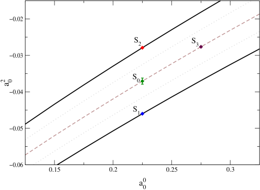
Figure 7: Universal band. The five lines correspond to the five different curves shown in fig. 5 (the top line, for instance, results if the input for ${\rm Im}\,t_{0}^{2}$ in the region above 0.8 GeV is taken from the top curve in that figure). $S_{0}$ marks our reference point: $a_{0}^{2}=0.225$, $a_{0}^{2}=-0.0371$. The bar attached to it indicates the uncertainty in $a_{0}^{2}$ due to the one in the phase $\delta_{0}^{0}$ at the matching point – the most important remaining source of error if the input for ${\rm Im}\,t_{0}^{2}$ is held fixed.

We now turn to the dependence of the universal curve $a_{0}^{2}=F(a_{0}^{0})$ on the input in the $I=0$ and $I=1$ channels, keeping the one for $I=2$ fixed. Changes in the input above $2M_{K}$ are practically invisible at threshold: If we keep the phase shifts at the matching point fixed, the three different available inputs for the $I=0$ and $I=1$ channels yield values of $a_{0}^{2}$ that differ by less than one permille. The phase shifts at $s_{0}$ are the only relevant factor here. Moreover, for the value of $a^{2}_{0}$, $\delta_{0}^{0}(s_{0})$ is much more important than $\delta^{1}_{1}(s_{0})$: Shifts of $\delta_{1}^{1}(s_{0})$ by $\pm 2^{\circ}$ change the value of $a_{0}^{2}$ roughly by a permille, but a change by $\pm 3.4^{\circ}$ in $\delta_{0}^{0}(s_{0})$ induces a shift of $\Delta a_{0}^{2}=\pm 8.4\cdot 10^{-4}$, which amounts to two percent. Even so, this is much smaller than the width of the band, as can be seen in fig. 7.

We have also varied $\sqrt{\rule[1.00006pt]{0.0pt}{5.0pt}s_{0}}$ within the bounds 0.78 and 0.86 GeV and found that the dependence of the relation $a_{0}^{2}=F(a_{0}^{0})$ on $s_{0}$ is rather weak. To exemplify, we mention that for the solution with $a_{0}^{0}=0.25$ at the center of the universal band, a shift from $\sqrt{\rule[1.00006pt]{0.0pt}{5.0pt}s_{0}}=0.8$ GeV to 0.85 GeV changes $a_{0}^{2}$ by $10^{-3}$.

10 Consistency

It takes a good balancing of the various terms occurring in the Roy equations for the partial waves not to violate the unitarity limit. In the case of the $S$-wave with $I=0$, for instance, the contribution to $\mbox{Re}\,t_{0}^{0}$ that arises from the subtraction term $k_{0}^{0}(s)$ is very large already at 1 GeV: The solution shown in fig. 6 corresponds to $a_{0}^{0}=0.225$ and $a_{0}^{2}=-0.0371$, so that $k_{0}^{0}(s)=2.7$ for $s=1\,\mbox{GeV}^{2}$. As the energy grows, the term increases and reaches $k_{0}^{0}(s_{1})=3.6$ at the upper end of the region where our equations are valid, $s_{1}=68\,M_{\pi}^{2}$. Unless the contributions from the dispersion integrals nearly compensate the subtraction term, the unitarity limit, $|\,\mbox{Re}\,t_{0}^{0}\,|\leq(2\sigma)^{-1}\simeq\frac{1}{2}$ is violated. The example in fig. 6 demonstrates that we do find solutions for which such a cancellation takes place, with values of $a_{0}^{0}$, $a_{0}^{2}$ that are within the universal band.

It is striking that, above the matching point, this solution very closely follows the real part of the input. In a restricted sense, this is necessary for the solution to be acceptable physically: The solution is obtained by identifying the imaginary part above the matching point with the one obtained from a particular representation of the partial waves. The Roy equations then determine the real part of the amplitude in the region below $\sqrt{\rule[1.00006pt]{0.0pt}{5.0pt}s_{1}}=1.15\,\mbox{GeV}$. If the result were very different from the real part of the particular representation used, we would have to conclude that this representation cannot properly describe the physics. This amounts to a consistency condition: Above the matching point, the Roy solution should not strongly deviate from the real part of the input. The condition can be met only if the cancellation discussed above takes place, but it is stronger. The example in fig. 6 demonstrates that there are solutions that obey the consistency condition remarkably well, indicating that our apparatus is indeed working properly.

We will discuss the consistency condition on a quantitative level below. Before entering this discussion, we briefly comment on a different aspect of our framework: the stability of the solutions. The behaviour below 0.8 GeV is not sensitive to the uncertainties in the input used for the imaginary parts above 1 GeV. We can modify that part of the input quite substantially, and without changing anything else (not even below $s_{0}$) still get a decent solution from threshold up to the limit of validity of our equations. Naturally, if we do not modify the Schenk parameters that define the phase below $s_{0}$, the Roy equations are not strictly obeyed, but the deviation from the true solution is quite small. The reason is that, if $s$ is small, the kernels $K^{II^{\prime}}_{\ell\ell^{\prime}}(s,s^{\prime})$ strongly suppress the contributions from the region where $s^{\prime}$ is large. The term $K^{00}_{00}(s,s^{\prime})$, for instance, has the following expansion for $s^{\prime}\gg s$:

$$K^{00}_{00}(s,s^{\prime})={1\over 9}\left\{11s^{2}-10s(4M_{\pi}^{2})-(4M_{\pi}^{2})^{2}\right\}{1\over s^{\prime\,3}}+O\left(\frac{1}{s^{\prime\,4}}\right)\;\;.$$

The interval above 1 GeV only generates very small contributions to the integrals on the r.h.s. of the Roy equations, if these are evaluated in the region below the matching point.

We now take up the consistency condition and first observe that, once a solution has a consistent behaviour above the matching point, reasonable changes in the input above 1 GeV lead to solutions that also obey the consistency condition: It looks as if the Roy equations were almost trivially satisfied, behaving like an identity for $E>1$ GeV. Is this consistent behaviour automatic, or does it depend crucially on part of the input ?

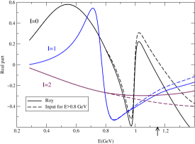
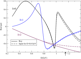
Figure 8: Solutions of the Roy equations for $a_{0}^{0}=0.225$ and two extreme values for $a_{0}^{2}$. The left figure corresponds to the point $S_{2}$ in fig.7, while the one on the right shows the solution for $S_{1}$. The arrows indicate the limit of validity of the Roy equations.

The answer to this question can be found in fig. 8, where we show two solutions obtained with the same value of $a_{0}^{0}$ as in fig. 6, but different inputs for ${\rm Im}\,t_{0}^{2}$: The solution on the left is obtained by using the top curve in fig. 5 instead of the central one ($a_{0}^{2}=-0.0279$ instead of $a_{0}^{2}=-0.0371$). The solution on the right corresponds to the bottom curve in fig. 5, where $a_{0}^{2}=-0.0460$. The figure clearly shows that the consistent picture which we have at the center of the universal band is almost completely lost if we go to the upper border of this band: It is by no means trivial that we at all find solutions for which the output is consistent with the input.

The fact that the peaks and valleys seen in the solutions mimic those in the input can be understood on the basis of analyticity alone: The curvature above the matching point arises from the behaviour of the imaginary parts there. The relevant term is the one from the principal value integral,

$$\mbox{Re}\,t(s)=\frac{1}{\pi}-\int_{4M_{\pi}^{2}}^{s_{2}}ds^{\prime}\,\frac{\mbox{Im}\,t(s^{\prime})}{s^{\prime}-s}+r(s)\;\;.$$

The remainder, $r(s)$ contains the contributions associated with the subtraction polynomial, the left hand cut, the higher partial waves, as well as the asymptotic region. On the interval $s_{0}<s<s_{1}$, it varies only slowly and is well approximated by a first order polynomial in $s$.

The representations of the partial wave amplitudes that we are using as an input are specified in terms of simple functions. In the vicinity of the region where we are comparing their real parts with the Roy solutions, these are analytic in $s$, except for the cut along the positive real axis. Hence they also admit an approximate representation of the above form – the contributions from distant singularities are well approximated by a first order polynomial. Disregarding the interpolation needed to match the representation with the prescribed value of the phase at $s_{0}$, their imaginary parts coincide with the one of the corresponding Roy solution above the matching point. The small differences occurring in the interpolation region and below the matching point do not generate an important difference in the curvature. We conclude that the difference between the Roy solution and the real part of the input must be linear in $s$, to a good approximation. Moreover, within the accuracy to which our solutions obey the Roy equations, the two expressions agree at the matching point, by construction. Accordingly, the relation can be written in the form

$$\mbox{Re}\,t(s)\rule[-3.00003pt]{1.00006pt}{0.0pt}_{\mbox{\tiny Roy}}=\mbox{Re}\,t(s)\rule[-3.00003pt]{1.00006pt}{0.0pt}_{\mbox{\tiny input}}+(s-s_{0})\,\beta\;\;.$$ (10.1)

We have checked that this relation indeed holds to sufficient accuracy, for all three partial waves. This does not yet explain why the solution follows the real part of the input, but shows that it must do so up to a term linear in $s$ that vanishes at the matching point. In particular, if the difference between input and output is small at the upper end of validity of our equations, then analyticity ensures that the same is true in the entire region between the matching point and that energy (in this interval, $s$ varies by about a factor of two).

In view of the uncertainties attached to our input, we cannot require the Roy equations to be strictly satisfied also above the matching point. The band spanned by the two green lines in fig. 9 shows the region in the $(a_{0}^{0},a_{0}^{2}$) plane, where the solution for $\mbox{Re}\,t_{0}^{0}(s)$ differs from the real part of the input by less than 0.05 (expressed in terms of the parameter $\beta$ in eq. (10.1), this amounts to $|\beta^{0}_{0}|<0.07\,\mbox{GeV}^{-2}$). Likewise, the band spanned by the two blue lines represents the region where $|\mbox{Re}\,t_{0}^{2}(s)_{\mbox{\tiny Roy}}-\mbox{Re}\,t_{0}^{2}(s)_{\mbox{\tiny input}}|<0.05$, so that $|\beta^{2}_{0}|<0.07\,\mbox{GeV}^{-2}$. The corresponding band for the $P$-wave is much broader – in this channel, the consistency condition is rather weak and is met everywhere inside the universal band. We conclude that, in the lower half of the universal band, all three waves show a consistent behaviour, while for the upper quarter of the band, this is not the case (the situation at the upper border is shown on the left in fig. 8).

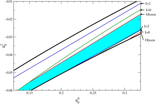
Figure 9: Regions inside which the consistency condition is met. The band between the two blue lines is for the condition in the $I=2$ channel, whereas the one between the two green lines is for the $I=0$ channel. The two red lines delimit the band inside which the Olsson sum rule is satisfied. The shaded area gives the intersection of the three bands.

It is not difficult to understand why the consistency condition is strongest for the $I=0$ $S$-wave. In this connection, the most important term in the Roy equations is the one from the subtraction polynomial – the solution can satisfy the consistency condition only if the term proportional to $s$ is nearly cancelled by a linear growth of the remaining contributions. The term generates the contribution $(\beta_{0}^{0},\beta_{1}^{1},\beta^{2}_{0})=(6,1,-3)\times(2a_{0}^{2}-5a_{0}^{2})/(72\,M_{\pi}^{2})$ to the coefficients that describe the difference between output and input for the three lowest partial waves. The subtraction polynomial thus contributes twice as much to $\beta_{0}^{0}$ as to $\beta^{2}_{0}$, so that the consistency band for the $I=2$ wave must be about twice as broad as the one for the $I=0$ wave, while the one for the $P$-wave must roughly be six times broader. At the qualitative level, these features are indeed born out in the figure, but we stress that the term from the subtraction polynomial is not the only one that matters – those arising from the integrals also depend on the values of $a_{0}^{0}$ and $a^{2}_{0}$. The two green lines correspond to a variation in $a^{2}_{0}$ by about $\pm 0.004$. Increasing $a^{2}_{0}$ by 0.004, the value of the subtraction term $k_{0}^{2}(s_{1})$ decreases by 0.10. The fact that the lines correspond to a change in $\mbox{Re}\,t^{0}_{0}(s_{1})$ of only $\pm 0.05$ implies that the contributions from the integrals reduce the shift by a factor of 2. Also, if only the subtraction term were relevant, the consistency bands would be determined by the combination $2a_{0}^{2}-5a_{0}^{2}$ and thus have a slope of $\frac{2}{5}$. Actually, these bands are roughly parallel to the universal band, whose slope is positive, but smaller by about a factor of 2.

11 Olsson sum rule

In the Roy equations, the imaginary parts above the matching point and the two subtraction constants $a_{0}^{0}$, $a_{0}^{2}$ appear as independent quantities. The consistency condition interrelates the two in such a manner that the contributions from the integrals over the imaginary parts nearly cancel the one from the subtraction term. In fact, a relation of this type can be derived on general grounds.

The fixed-$t$ dispersion relation (2) contains two subtractions. In principle, one subtraction suffices, for the following reason. The $t$-channel $I=1$ amplitude

$$T^{(1)}(s,t)\equiv\frac{1}{6}\,\{2\,T^{0}(s,t)+3\,T^{1}(s,t)-5\,T^{2}(s,t)\}$$

does not receive a Pomeron contribution and thus only grows in proportion to $s^{\alpha_{\rho}(t)}$ for $s\rightarrow\infty$. The dispersion relation (2.4), however, does contain terms that grow linearly with $s$. For the relation to be consistent with Regge asymptotics, the contribution from the subtraction term must cancel the one from the dispersion integral. At $t=0$, this condition reduces to the Olsson sum rule, which relates the subtraction constants to an integral over the imaginary parts [67]:

$$2\,a_{0}^{0}-5\,a_{0}^{2} \!\!\!\!= \!\!\!\!\frac{M_{\pi}^{2}}{8\pi^{2}}\int_{4M_{\pi}^{2}}^{\infty}\!ds\;\frac{2\,\mbox{Im}\,T^{0}(s,0)+3\,\mbox{Im}\,T^{1}(s,0)-5\,\mbox{Im}\,T^{2}(s,0)}{s\,(s-4M_{\pi}^{2})}\,.$$ (11.1)

It is well known that this sum rule converges only slowly – the contributions from the asymptotic region cannot be neglected. We split the integral into four pieces,

$$2\,a_{0}^{0}-5\,a_{0}^{2}=O_{\scriptscriptstyle SP}+O_{\scriptscriptstyle D}+O_{\scriptscriptstyle F}+O_{as}\;\;.$$

The first term represents the contributions from the imaginary parts of the $S$- and $P$-waves in the region below 2 GeV, which are readily worked out, using our Roy solutions on the interval from threshold to 0.8 GeV and the input phase shifts on the remainder. The result is not very sensitive to the input used and is well approximated by a linear dependence on the scattering lengths,

$$O_{\scriptscriptstyle SP}=0.483\pm 0.011\,+1.13\,(a_{0}^{0}-0.225)-1.01\,(a^{2}_{0}+0.0371)\;\;.$$

The remainder is closely related to the moments $I^{I}_{n}$ introduced in appendix B.1: here, we are concerned with the case $n=-1$. The term $O_{\scriptscriptstyle D}$ describes the contribution from the imaginary part of the $D$-waves, in the interval from threshold to 2 GeV. The relevant experimental information is discussed in appendix B.3, where we also explain how we estimate the uncertainties. The numerical result reads $O_{\scriptscriptstyle D}=0.061\pm 0.004$, including the small, negative contribution from the $I=2$ $D$-wave. The bulk stems from the tensor meson $f_{2}(1275)$: In the narrow width approximation, this contribution amounts to 0.063. For the analogous contribution due to the $F$-wave, we obtain $O_{\scriptscriptstyle F}=0.017\pm 0.002$ (in narrow width approximation, the term generated by the $\rho_{3}(1690)$ yields 0.013). Those from the asymptotic region are dominated by the leading Regge trajectory – as noted above, the Pomeron does not contribute. Evaluating the asymptotic contributions with the formulae given in appendix B.4, we obtain $O_{as}=0.102\pm 0.017$. Collecting terms, this yields

$$2\,a_{0}^{0}-5\,a_{0}^{2}=0.663\pm 0.021+1.13\,(a_{0}^{0}-0.225)-1.01\,(a^{2}_{0}+0.0371)\;\;.$$ (11.2)

The result corresponds to a band in the $(a_{0}^{0},a_{0}^{2})$ plane:

$$a^{2}_{0}=-0.044\pm 0.005+0.218\,(a_{0}^{0}-0.225)\;\;.$$ (11.3)

The band is spanned by the two red lines shown in fig. 9. One of these nearly coincides with the lower border of the universal band, while the other runs near the center. The Olsson sum rule thus imposes roughly the same relation between $a^{0}_{0}$ and $a^{2}_{0}$ as the consistency condition. Note that the asymptotic contributions are numerically quite important here: The term $O_{as}$ amounts to a shift in $a^{2}_{0}$ of $-0.026\pm 0.004$. The fact that – in the region where our solutions are internally consistent – the sum rule is indeed obeyed, represents a good check on our asymptotics.

The Olsson sum rule ensures the proper asymptotic behaviour of the amplitude only for $t=0$. In order for the terms that grow linearly with $s$ to cancel also for $t\neq 0$, the imaginary part of the $P$-wave must obey an entire family of sum rules. The matter is discussed in detail in appendix C.1, where we demonstrate that one of these offers a further, rather sensitive test of our framework. The relationship between the Roy equations and those proposed by Chew and Mandelstam [68] is described in appendix C.2, where we also comment on the asymptotic behaviour of the dispersion integrals that occur on the r.h.s. of the Roy equations for the $S$- and $P$-waves.

12 Comparison with experimental data

In our framework, the only free parameter is $a_{0}^{0}$. Comparing our Roy equation solutions to data, we can determine the range of $a_{0}^{0}$ consistent with these, as well as a corresponding range for $a_{0}^{2}$. This experimental determination of the two $S$-wave scattering lengths is the final scope of the present analysis and the main subject of the present section. Data on the $\pi\pi$ amplitude are available in a rather wide range of energies (we do not indicate the upper limit in energy when this exceeds 1.15 GeV, the limit of validity of our equations):

• $K_{e4}$ data for the combination $\delta_{0}^{0}-\delta_{1}^{1}$ ($2M_{\pi}\leq E\leq 0.37$ GeV);

• ACM and Losty et al. data for $\delta_{0}^{2}$ (0.35 GeV $\leq E$);

• Data on the vector form factor – according to the discussion in section 7.3, these can safely be converted into values for $\delta_{1}^{1}$ in the region of the $\rho$ ($0.5\leq E\leq 0.9$ GeV);

• CERN–Munich, and Berkeley data in the channels with $I=0$ and $I=1$ (0.5 GeV $\leq E$);

In the Roy equations, $a_{0}^{0}$ and $a^{2}_{0}$ exclusively enter through the subtraction polynomials, specified in eq. (1.2). Those relevant for the $S$-waves contain a constant contribution given by the scattering length and a term proportional to $(s-4M_{\pi}^{2})\times(2a^{0}_{0}-5a_{0}^{2})$. In the $I=0$ wave, that term is larger than $a_{0}^{0}$ from $E\sim 0.5$ GeV on. For the $I=2$ wave, the linear term starts dominating over $a_{0}^{2}$ even earlier. Since $t^{1}_{1}(s)$ vanishes at threshold, the corresponding subtraction polynomial exclusively involves the linear term. This implies that, except in the vicinity of threshold, the behaviour of the solutions is sensitive only to the combination $2a_{0}^{0}-5a_{0}^{2}$ of scattering lengths – roughly the combination that characterizes the universal band. Accordingly, only data that reach down close to threshold give a direct handle to separately determine $a_{0}^{0}$ and $a_{0}^{2}$. In fact, only those coming from $K_{e4}$ decays meet this condition.

There is another threshold in energy that is obviously relevant for our approach: the matching point $s_{0}$. We will make a clear distinction between data points below $s_{0}$ and those at higher energies. The comparison to data above $s_{0}$ can hardly yield any information on the scattering lengths, because the behaviour of our solutions at those energies very strongly depends on the input used for the imaginary parts: The uncertainties in the experimental input completely cover the dependence of the solutions on the scattering lengths – we will discuss this in detail below. Instead, we analyze the requirement that the solution is consistent with the input for $s>s_{0}$, in the sense discussed in section 10. This condition turns out to be practically independent of the input used for the imaginary parts above $s_{0}$ and does therefore yield a meaningful constraint on $2a_{0}^{0}-5a_{0}^{2}$.

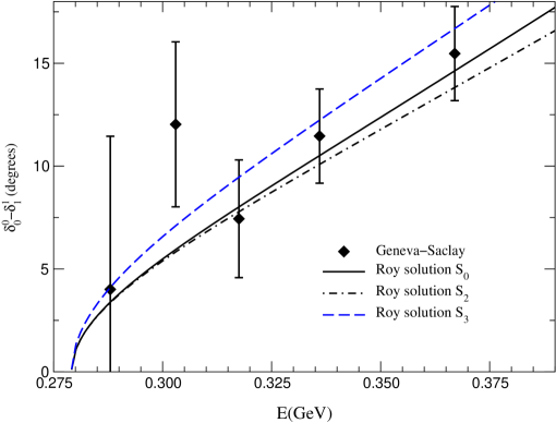
Figure 10: Comparison of our Roy solutions for different values of the scattering lengths with the data of the Geneva–Saclay collaboration, Rosselet et al. [69]. The full, dash-dotted and dashed lines correspond to the points $S_{0}$, $S_{2}$ and $S_{3}$ in fig. 7.

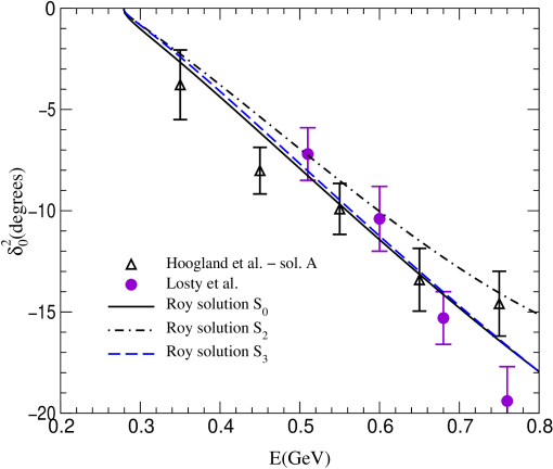
Figure 11: Comparison of our Roy solutions with the data on $\delta^{2}_{0}$ obtained by the ACM collaboration [53] and by Losty et al. [51]. The full, dash-dotted and dashed lines correspond to the points $S_{0}$, $S_{2}$ and $S_{3}$ in fig. 7.

12.1 Data on $\delta_{0}^{0}-\delta_{1}^{1}$ from $K_{e4}$, and on $\delta_{0}^{2}$ below 0.8 GeV

Let us first consider the $K_{e4}$ data. The comparison between our solutions and the high-statistic data of the Geneva–Saclay collaboration [69] is shown in fig. 10, for various values of the scattering lengths. The figure confirms the simple intuition that these data are mainly sensitive to $a_{0}^{0}$. In accordance with previous analyses [75], we find that they roughly constrain $a_{0}^{0}$ to the range between $0.18$ and $0.3$.

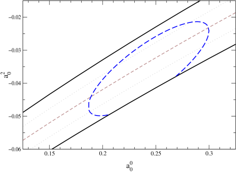
Figure 12: Range selected by the data below 0.8 GeV. The dashed line represents the 68% C.L. contour obtained by combining the Geneva–Saclay data on $K_{e4}$ decay with those from ACM(A) on $\delta_{0}^{2}$.

As for the low–energy data in the $I=2$ channel, we should stress that this wave is quite strongly constrained once $\delta_{0}^{2}(s_{0})$ is fixed. Because of the absence of any structures between threshold and 0.8 GeV, once we fix $\delta_{0}^{2}(s_{0})$, the only freedom is in the way the phase approaches zero at threshold, i.e. in the value of $a_{0}^{2}$ – which depends on $a_{0}^{0}$. Fig. 11 shows that, at fixed $\delta_{0}^{2}(s_{0})$, even a sizeable change in $a_{0}^{0}$ is barely visible in the $I=2$ phase. The only important factor here is the value of the phase at the matching point: The comparison with the experimental data basically tells us which value of $\delta_{0}^{2}(s_{0})$ is preferred.

A quantitative statement can be made in terms of $\chi^{2}$, and in principle we could calculate three different $\chi^{2}$-values, based on the three sets of data shown in fig. 5. Two of these, however, represent two different analyses of the same set of $\pi N\to\pi\pi N$ data. Their difference is a clear sign of the presence of sizeable systematic errors. We have estimated the latter using the difference, point by point, between the two analyses A and B of ref. [53], and added this in quadrature to the statistical errors. As reference we have used the ACM(A) set of data, but have checked that interchanging it with the one of Losty et al. does not give significantly different results. The corresponding $\chi^{2}$, combined with the one obtained from the $K_{e4}$ data, has a minimum $\chi^{2}_{min}=5.1$ (with 8 d.o.f.) at $a_{0}^{0}=0.242$, $a_{0}^{2}=-0.0357$. The contour corresponding to 68% confidence level ($\chi^{2}=\chi^{2}_{min}+2.3$) is shown in fig. 12: The range $0.18<a_{0}^{0}<0.3$ is dictated by the $K_{e4}$ data, whereas the $I=2$ data exclude the upper border of the band.

12.2 The $\rho$ resonance.

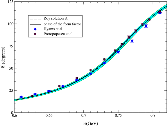
Figure 13: P-wave phase shift. The band shows the result of our analysis, obtained by varying the input within its uncertainties, while the data points indicate the phase shift measured in the process $\pi N\rightarrow\pi\pi N$ by the CERN-Munich collaboration. The full line represents the phase of the vector form factor (Gounaris-Sakurai fit of ref. [64]).

The input used at the matching point implies that the $P$-wave phase shift must pass through $90^{\circ}$ somewhere between threshold and 0.8 GeV – the Roy equations determine the place where this happens and how rapidly the phase must grow with the energy there. The solutions turn out to be very stiff: Varying the values of $a_{0}^{0}$ and $a_{0}^{2}$ within the universal band, and also varying the input for the imaginary parts above 0.8 GeV within the experimental uncertainties, we obtain the narrow band of solutions shown in fig. 13.

In this figure, the energy range only extends to $0.82\,\mbox{GeV}$, for the following reason: Our solutions move along the Argand circle only below the matching point. At higher energies, the real part of the partial wave calculated from the Roy equations does not exactly match the imaginary part used as an input: unless we correct the latter, the elasticity $\eta_{1}^{1}$ differs from unity, already before the inelastic channels start making a significant contribution. If the consistency condition is met well, the departure from unity is small, but it can become as large as 5% if we go to the extreme of the consistency region shown in fig.9. This means that it does not make much sense to extract the value of the phase without adjusting the imaginary part. The proper way to do this is to extend the interval on which the Roy equations are solved, but we did not carry this out.

In the region $0.7\,\mbox{GeV}<0.82\,\mbox{GeV}$, the result closely follows the data of the CERN-Munich collaboration. Below 0.7 GeV, however, the data are in conflict with the outcome of our analysis: The five lowest data points are outside the range allowed by the Roy equations, a problem noted already in ref. [6]. In our opinion, we are using a generous estimate of the uncertainties to be attached to our input. Note, in particular, that at those energies, the driving terms barely contribute. We conclude that the discrepancy between our result and the CERN-Munich phase shift analysis occurring on the left wing of the $\rho$ is likely to be attributed to an underestimate of the experimental errors. As discussed below, the comparison with the $e^{+}e^{-}$ and $\tau$ decay data corroborates this conclusion.

Concerning the resonance parameters, we first give the ranges of mass and width that follow if, in the vicinity of the resonance, the phase shift is approximated by a Breit-Wigner formula

$$e^{2\,i\,\delta_{1}^{1}(s)}=\frac{M^{2}_{\rho}+i\,\Gamma_{\rho}M_{\rho}-s}{M_{\rho}^{2}-i\,\Gamma_{\rho}M_{\rho}-s}\;\;,\hskip 20.00003pt\mbox{tg}\,\delta_{1}^{1}(s)=\frac{\Gamma_{\rho}M_{\rho}}{M_{\rho}^{2}-s}\;\;.$$

In this approximation, the mass of the resonance is the real value of the energy where the phase passes through $90^{\circ}$ and the width may be determined from the value of the slope $d\delta^{1}_{1}/ds$ at resonance. The solutions contained in the band shown in the figure correspond to the range $M_{\rho}=774\pm 3\,\mbox{MeV}$ and $\Gamma_{\rho}=145\pm 7\,\mbox{MeV}$, to be compared with the average values obtained by the Particle Data Group, $M_{\rho}=770.0\pm 0.8\,\mbox{MeV}$, $\Gamma_{\rho}=150.7\pm 1.1\,\mbox{MeV}$ [70].

The only process independent property of the resonance is the position of the corresponding pole – the above numbers specify this position only approximately. To determine it more accurately, we first observe that the Roy equations yield a representation of the partial wave $t_{1}^{1}(s)$ on the first sheet, in terms of the imaginary parts along the real axis. The first sheet contains both a right and a left hand cut. We need to analytically continue the function from the upper rim of the right hand cut into the lower half plane (second sheet). The difference between the values obtained in this manner and those found by evaluating the Roy representation in the lower half plane is given by the analytic continuation of the imaginary part,

$$\mbox{Im}\,t_{1}^{1}(s)=\frac{1}{\sigma(s)}\,\sin^{2}\!\delta_{1}^{1}(s)\;\;.$$

On the first sheet, $t_{1}^{1}(s)$ does not have singularities. Hence a pole can only arise from the continuation of the imaginary part. Indeed, the function $\sin^{2}\!\delta_{1}^{1}(s)$ contains the term $\exp 2\,i\,\delta_{1}^{1}(s)$, which has a pole below the real axis. The position is readily worked out with the explicit, algebraic parametrization of the phase that we are using. The result illustrates an observation made long ago [71, 72, 73]: The pole mass is lower than the energy at which the phase goes through $90^{\circ}$, by about 10 MeV: For the band shown in the figure, the pole position varies in the range

$$M_{\rho}=762.5\pm 2\,\mbox{MeV}\;\;,\hskip 20.00003pt\Gamma_{\rho}=142\pm 7\,\mbox{MeV}\;\;.$$

The $e^{+}e^{-}$ and $\tau$ data neatly confirm the conclusion reached above: The phase of the form factor is in perfect agreement with the behaviour of the $P$-wave that follows from the Roy equations, but differs from the data of the CERN-Munich phase shift analysis, particularly below 0.7 GeV. In our opinion, the information obtained about the behaviour on the left wing of the resonance on the basis of the reactions $e^{+}e^{-}\rightarrow\pi^{+}\pi^{-}$ and $\tau\rightarrow\pi^{-}\pi^{0}\nu$ is more reliable than the one obtained from $\pi N\rightarrow\pi\pi N$. The fact that the Roy equations are in good agreement with the $e^{+}e^{-}$ and $\tau$ data is very encouraging.

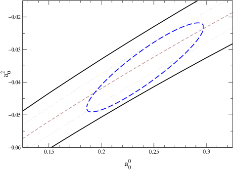
Figure 14: 68% C.L. contour obtained by combining all relevant low energy data: $K_{e4}$ decay, ACM(A) data on $\delta_{0}^{2}$ below 0.8 GeV and results for $\delta_{1}^{1}$ extracted from the $e^{+}e^{-}$ and $\tau$ data on the pion form factor.

In view of the clean determination of the $P$-wave phase shift through $e^{+}e^{-}$ and $\tau$ experiments, we find it instructive to draw fixed $\chi^{2}$-contours in the $(a_{0}^{0},a_{0}^{2})$ plane. To do so, we first need to attach an error bar to the curve representing the phase shift. In section 7.4, we estimated the uncertainty in $\delta_{1}^{1}(s_{0})$ at $\pm 2^{\circ}$ or $\pm 2\%$. As we go down in energy, the relative precision of the determination of the phase decreases: A generous estimate of the uncertainty at $\sqrt{s}=0.5$ GeV is 10% or $\pm 0.6^{\circ}$. A smooth interpolation between these two values is our estimate of the experimental error bar (below that energy, the $e^{+}e^{-}$ and $\tau$ data become scarce and have sizeable uncertainties). To construct the $\chi^{2}$ we have compared our solutions to the experimentally determined phase shift at five points between 0.5 and 0.75 GeV. Combining this $\chi^{2}$ with those from the data on $K_{e4}$ decays and on $\delta_{0}^{2}$ below 0.8 GeV, we obtain the 68% C.L. area drawn in fig. 14. The minimum of the $\chi^{2}$ is now 5.4 (with 13 d.o.f.). The position of the minimum is barely shifted: It now occurs at $a_{0}^{0}=0.240$, $a_{0}^{2}=-0.0356$. In other words, at the place where the $\chi^{2}$ of the $K_{e4}$ data on $\delta_{0}^{0}-\delta_{1}^{1}$ and those on $\delta_{0}^{2}$ had a minimum, the $\chi^{2}$ relative to the data on the form factor is practically zero and also has a minimum. In view of the fact that the uncertainties in $\delta_{1}^{1}$ are very small, this is quite remarkable. The data on the $P$-wave do not change the position of the minimum, but shrink the ellipse along the width of the universal band. As expected, they do not reduce the range of allowed values of $a_{0}^{0}$.

12.3 Data on the $I=0$ $S$-wave below 0.8 GeV

In fig. 15 we compare the $S$-wave obtained from our Roy equation solutions with the available data: CERN-Munich [47] and Berkeley [48]. The band shown is a representation of the uncertainties in the solution, which have two main sources: the uncertainty in $\delta_{0}^{0}(s_{0})$ and the one in $\delta^{2}_{0}(s_{0})$ (width of the universal band). The central curve shows our reference solution $a_{0}^{0}=0.225$, $a_{0}^{2}=-0.0371$. The uncertainties indicated do not account for the changes occurring if the value $a_{0}^{0}=0.225$ is modified. Changing this value within reasonable bounds, however, brings the solution out of the band only below 0.4 GeV, already far below the first data point. The figure shows good agreement with the data, especially so for the Berkeley data set. The CERN-Munich data set shows a certain structure, which does not occur in our solutions – in view of the uncertainties in the data, this difference does not represent a problem.

Despite the positive picture which emerges from the comparison, we refrain from using these data to draw confidence–level contours in the $(a_{0}^{0},a_{0}^{2})$ plane. The $S$-wave phase shifts have been extracted simultaneously with the $P$-wave. As discussed in the preceding section, these are affected by systematic errors which are at least as large as the statistical ones. The same must be true for the data in the $I=0$ channel, so that a quantitative comparison with the Roy solutions is barely significant.

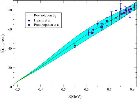
Figure 15: Comparison between the Roy solution for the $S$-wave and the phase shift analyses of the CERN-Munich (circles) and Berkeley (squares) collaborations. The band shows the uncertainties in the Roy solution, which are dominated by those in $a_{0}^{0}$ and $a_{0}^{2}$.

12.4 Data above 0.8 GeV

The Roy equations are valid up to $\sqrt{\rule[1.00006pt]{0.0pt}{5.0pt}s_{1}}=1.15$ GeV. In fig. 16, we show three different solutions for the $I=0$ and $I=1$ partial waves, in the region above the matching point. They are obtained by using three different inputs for the imaginary parts (note that the curves represent our solutions, not the real parts of the input). The figure shows that the differences are substantial, especially in the $S$-wave, despite the fact that, below $\sqrt{\rule[1.00006pt]{0.0pt}{5.0pt}s_{0}}=0.8\,\mbox{GeV}$, the three solutions are practically identical, for all three waves. Evidently, above the matching point, the Roy solutions are very sensitive to the input used for the imaginary parts.

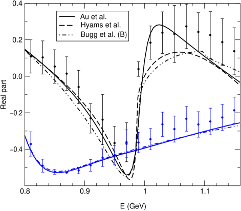
Figure 16: Behaviour of the solutions above the matching point. The curves show the solutions obtained with three different inputs for the imaginary parts. The data points are taken from the energy independent analysis of the CERN-Munich data [47]. The $I=0$ $S$-wave is shown in black, the $I=1$ $P$-wave in blue.

It is not difficult to understand why that is so. As discussed in detail in section 10, the solutions follow the real parts of the representation that is used as input (see fig. 6 for the case of Au et al. – in the other two cases, the picture is similar). The real parts of the three representations differ considerably. Moreover, all of these are systematically lower than the “data points” in fig. 16, which show the result of an energy independent analysis of the CERN-Munich data [47]. In view of this, it is not surprising that the three Roy solutions are quite different and that they are also systematically lower than the data points.

We conclude that a comparison of the Roy solutions with the data in the region above the matching point does not yield reliable information about the values of the two $S$-wave scattering lengths and we do therefore not show confidence–level contours relative to data above 0.8 GeV.

13 Allowed range for $a_{0}^{0}$ and $a_{0}^{2}$

The above discussion has made clear that we can rely only on two rather solid sources of experimental information to determine the two $S$-wave scattering lengths: the data on $K_{e4}$ and those on the $P$-wave in the $\rho$ region. The former determine a range of allowed values for $a_{0}^{0}$ while the latter yield a range for the combination $2a_{0}^{0}-5a_{0}^{2}$. The consistency condition and the Olsson sum rule impose further constraints. Figure 17 summarizes our findings: We have superimposed the ellipse of fig. 14 with the lines that delimit the consistency bands for the two $S$-waves, as well as those relevant for the Olsson sum rule. The allowed range for $a_{0}^{0}$ and $a_{0}^{2}$ is the intersection of the ellipse with the band where the Olsson sum rule is obeyed within the estimated errors. In that region, the solutions also satisfy the consistency condition.

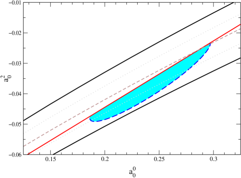
Figure 17: Intersection of the ellipse in fig. 14 (68% C.L. relative to the data on $K_{e4}$ decay, on $\delta_{0}^{2}$ and on the form factor) with the bands allowed by the consistency condition in all the three channels and by the Olsson sum rule.

We find it quite remarkable that the data on the shape of the $\rho$ resonance, the consistency condition and the Olsson sum rule all show a preference for the lower part of the universal band. This gives us confidence that our conclusion on which region in the $(a_{0}^{0},a_{0}^{2})$ plane is allowed by the present experimental information is rather solid. Once the new data on $K_{e4}$ decays will become available, the allowed range in $a_{0}^{0}$ will become much narrower, and we will have a very small ellipse. The prospects of making a real precision test of the predictions for the two $S$-wave scattering lengths in the near future, appear to be very good, in particular also in view of the pionium experiment under way at CERN [29].

The $\pi N\rightarrow\pi\pi N$ data do provide essential information concerning the input of our calculations, but, as discussed in sections 12.3 and 12.4, they do not impose a firm constraint on the scattering lengths (incidentally, these data also prefer the lower half of the universal band). This is unfortunate, because the power of the Roy equations (unitarity, crossing symmetry and analyticity) is that of connecting regions of very different energy scales. The behaviour of the two $S$-waves in the immediate vicinity of threshold is determined by the scattering lengths. In the combination $2a_{0}^{0}-5a_{0}^{2}$, these also determine the linear growth of the subtraction polynomial: As we discussed in detail in section 10, the large contribution from the polynomial must be compensated to a high degree of accuracy by the dispersive integrals. We therefore expect that a reanalysis of the $\pi N\rightarrow\pi\pi N$ data based on the Roy equations would lead to a rather stringent constraint on the allowed region, as it would make full use of the information contained in these data – in our opinion, the existing phase shift analyses are a comparatively poor substitute.

14 Threshold parameters

14.1 $S$- and $P$-waves

As shown in ref. [74], the effective ranges of the $S$- and $P$-waves and the $P$-wave scattering length can be expressed in the form of sum rules, involving integrals over the imaginary parts of the scattering amplitude and the combination $2a_{0}^{0}-5a_{0}^{2}$ of $S$-wave scattering lengths. The sum rules may be derived from the Roy representation by expanding the r.h.s. of eq. (5.1) in $q^{2}$ and reading off the coefficients according to eq. (2.3). In the case of the $S$-wave effective ranges, the expansion can be interchanged with the integration over the imaginary parts only after removing the threshold singularity. This can be done by supplementing the integrand with a term proportional to the derivative

$$\frac{d}{ds}\,\frac{1}{\sqrt{s(s-4\,M_{\pi}^{2})}}=-\frac{h(s)}{\{s(s-4\,M_{\pi}^{2})\}^{2}}\;\;,\hskip 10.00002pth(s)=(s-2M_{\pi}^{2})\sqrt{s(s-4M_{\pi}^{2})}\;\;.$$

In this notation, the sum rules may be written in the form:

$$b_{0}^{0} \!\!\!\!= \!\!\!\!\frac{1}{3M_{\pi}^{2}}\,(2a_{0}^{0}-5a_{0}^{2})+\,\frac{16}{3\pi}\int_{4M_{\pi}^{2}}^{s_{2}}\frac{ds}{\{s(s-4M_{\pi}^{2})\}^{2}}\left\{4M_{\pi}^{2}(s-M_{\pi}^{2})\,\mbox{Im}\,t_{0}^{0}(s)\right.$$ (14.1)

$$\!\!\!\!\left.-\,9M_{\pi}^{2}(s-4M_{\pi}^{2})\,\mbox{Im}\,t_{1}^{1}(s)+\,5M_{\pi}^{2}(s-4M_{\pi}^{2})\,\mbox{Im}\,t_{0}^{2}(s)-\mbox{$\frac{3}{2}$}(a_{0}^{0})^{2}\,h(s)\right\}$$

$$\!\!\!\!-\frac{8}{\pi}\int_{s_{2}}^{\infty}\frac{ds}{\{s(s-4M_{\pi}^{2})\}^{2}}\,(a_{0}^{0})^{2}\,h(s)+b^{0}_{0\,d}\;\;,$$

$$b^{2}_{0} \!\!\!\!= \!\!\!\!-\frac{1}{6M_{\pi}^{2}}\,(2a_{0}^{0}-5a_{0}^{2})+\,\frac{8}{3\pi}\int_{4M_{\pi}^{2}}^{s_{2}}\frac{ds}{\{s(s-4M_{\pi}^{2})\}^{2}}\left\{2M_{\pi}^{2}(s-4M_{\pi}^{2})\,\mbox{Im}\,t_{0}^{0}(s)\right.$$

$$\!\!\!\!\left.+\,9M_{\pi}^{2}(s-4M_{\pi}^{2})\,\mbox{Im}\,t_{1}^{1}(s)+\,M_{\pi}^{2}(7s-4M_{\pi}^{2})\,\mbox{Im}\,t_{0}^{2}(s)-3(a_{0}^{2})^{2}\,h(s)\right\}$$

$$\!\!\!\!-\frac{8}{\pi}\int_{s_{2}}^{\infty}\frac{ds}{\{s(s-4M_{\pi}^{2})\}^{2}}\,(a_{0}^{2})^{2}\,h(s)+b^{2}_{0\,d}\;\;,$$

$$a^{1}_{1} \!\!\!\!= \!\!\!\!\frac{1}{18M_{\pi}^{2}}\,(2a^{0}_{0}-5a^{2}_{0})+\,\frac{8M_{\pi}^{2}}{9\pi}\int_{4M_{\pi}^{2}}^{s_{2}}\frac{ds}{\{s(s-4M_{\pi}^{2})\}^{2}}\left\{-2(s-4M_{\pi}^{2})\,\mbox{Im}\,t_{0}^{0}(s)\right.$$

$$\!\!\!\!\left.\hskip 56.9055pt+\,9(3s-4M_{\pi}^{2})\,\mbox{Im}\,t_{1}^{1}(s)+5(s-4M_{\pi}^{2})\,\mbox{Im}\,t_{0}^{2}(s)\right\}+a^{1}_{1\,d}\;\;,$$

$$b^{1}_{1} \!\!\!\!= \!\!\!\!\frac{8}{9\pi}\int_{4M_{\pi}^{2}}^{s_{2}}\frac{ds}{\{s(s-4M_{\pi}^{2})\}^{3}}\left\{-2(s-4M_{\pi}^{2})^{3}\,\mbox{Im}\,t_{0}^{0}(s)+9\left(\rule[-3.99994pt]{0.0pt}{10.00002pt}3\,s^{3}-12\,s^{2}M_{\pi}^{2}\right.\right.$$

$$\!\!\!\!\left.\left.\rule[-3.99994pt]{0.0pt}{10.00002pt}+\,48\,sM_{\pi}^{4}-64M_{\pi}^{6}\right)\,\mbox{Im}\,t_{1}^{1}(s)+5(s-4M_{\pi}^{2})^{3}\,\mbox{Im}\,t_{0}^{2}(s)\right\}+b^{1}_{1\,d}\;.$$

The integrals only involve the imaginary parts of the $S$- and $P$-waves and are cut off at $s=s_{2}$. The contributions from higher energies, as well as those from the imaginary parts of the partial waves with $\ell=2,3,\ldots$ are contained in the constants $b^{0}_{0\,d}$, $b^{2}_{0\,d}$, $a^{1}_{1\,d}$, $b^{1}_{1\,d}$. By construction, these represent derivatives of the driving terms at threshold, $d_{0}^{0}(s)=q^{2}b^{0}_{0\,d}+O(q^{4})\,,\hskip 5.0ptd^{1}_{1}(s)=q^{2}a^{1}_{1\,d}+q^{4}b^{1}_{1\,d}+O(q^{6})\,,\hskip 5.0ptd_{0}^{2}(s)=q^{2}b^{2}_{0\,d}+O(q^{4})\,.$ The numerical

	A	B	C	D	E	total	$\rule{8.00003pt}{0.0pt}\Delta_{1}$	$\rule{3.00003pt}{0.0pt}\Delta_{2}$	ref.[75]	units
$b^{0}_{0}$	2.12	$.45$	$-.03$	.02	.00	$2.56$	$\pm.02\rule{4.49997pt}{0.0pt}$	$\rule[-3.00003pt]{0.0pt}{13.99995pt}{}^{+.28}_{-.12}$	$2.5\pm 0.3$	$10^{-1}M_{\pi}^{-2}$
$b_{0}^{2}$	$-1.06$	$.26$	$.02$	.01	.00	$-.77$	$\pm.003$	$\rule[-3.00003pt]{0.0pt}{15.00002pt}{}_{-.07}^{+.03}$	$-.82\pm.08$	$10^{-1}M_{\pi}^{-2}$
$a_{1}^{1}$	3.53	$-.03$	$.13$	$-.01$	.01	$3.63$	$\pm.02\rule{4.49997pt}{0.0pt}$	$\rule[-3.00003pt]{0.0pt}{15.00002pt}{}_{-.11}^{+.29}$	$3.8\pm 0.2$	$10^{-2}M_{\pi}^{-2}$
$b_{1}^{1}$		$4.05$	$1.39$	$-.07$	.08	$5.45$	$\pm.13\rule{4.49997pt}{0.0pt}$	$\rule[-5.0pt]{0.0pt}{16.00008pt}{}_{-.44}^{+.35}$		$10^{-3}M_{\pi}^{-4}$
$a^{0}_{2}$		$1.29$	$.28$	.07	.03	$1.67$	$\pm.01\rule{3.99994pt}{0.0pt}$	$\rule[-3.99994pt]{0.0pt}{15.00002pt}{}_{-.06}^{+.15}$	$1.7\pm.3\rule{5.0pt}{0.0pt}$	$10^{-3}M_{\pi}^{-4}$
$b_{2}^{0}$		$-3.48$	$-.04$	.25	.02	$-3.25$	$\pm.07\rule{3.99994pt}{0.0pt}$	$\rule[-3.99994pt]{0.0pt}{15.00002pt}{}_{-.87}^{+.34}$		$10^{-4}M_{\pi}^{-6}$
$a^{2}_{2}$		$1.67$	$-.51$	.35	.02	$1.53$	$\pm.07\rule{3.99994pt}{0.0pt}$	$\rule[-3.99994pt]{0.0pt}{15.00002pt}{}_{-.45}^{+1.1}$	$1.3\pm 3\rule{7.5pt}{0.0pt}$	$10^{-4}M_{\pi}^{-4}$
$b^{2}_{2}$		$-3.10$	$-.09$	.06	.02	$-3.11$	$\pm.07\rule{3.99994pt}{0.0pt}$	$\rule[-3.99994pt]{0.0pt}{15.00002pt}{}_{-.95}^{+.41}$		$10^{-4}M_{\pi}^{-6}$
$a^{1}_{3}$		$5.11$	$.26$	.05	.01	$5.43$	$\pm.1\rule{8.00003pt}{0.0pt}$	$\rule[-3.99994pt]{0.0pt}{15.00002pt}{}_{-.72}^{+1.6}$	$6\pm 2\rule{7.5pt}{0.0pt}$	$10^{-5}M_{\pi}^{-6}$
$b^{1}_{3}$		$-3.96$	$-.01$	.01	.01	$-3.95$	$\pm.08\rule{3.99994pt}{0.0pt}$	$\rule[-5.0pt]{0.0pt}{15.00002pt}{}_{-1.9}^{+.89}$		$10^{-5}M_{\pi}^{-8}$

Table 4: Threshold parameters of the $S$-, $P$-, $D$- and $F$-waves. The significance of the entries in columns A–E is specified in the text. The column $\Delta_{1}$ indicates the uncertainty due to the error bars in the experimental input at and above 0.8 GeV, whereas $\Delta_{2}$ shows the shifts occurring if $a_{0}^{0}$ and $a_{0}^{2}$ are varied within the ellipse of fig. 14, according to eqs. (14.6) and (14.14).

values obtained within our framework are given in the upper half of table 4, where we also show the numbers quoted in the compilation of Nagels et al. [75], which are based on the analysis of Basdevant, Froggatt and Petersen [6]. In accordance with the literature, we use pion mass units. Since the relevant physical scale is of the order of 1 GeV, the numerical values rapidly decrease with the dimension of the quantity listed. The columns A – E indicate the following contributions to the total:

A. Contribution from the subtraction term $\propto 2a_{0}^{2}-5a_{0}^{2}$.

B. Imaginary parts of the $S$- and $P$-waves on the interval $4\,M_{\pi}^{2}<s<s_{0}$. This contribution is evaluated with the Roy solutions described in the text.

C. Imaginary parts of the $S$- and $P$-waves in the range $s_{0}<s<s_{2}$. Here, we are relying on the experimental information, discussed in section 7.

D. Imaginary parts of the higher partial waves in the range $4\,M_{\pi}^{2}<s<s_{2}$. These are calculated in the same manner as for the driving terms of the $S$- and $P$-waves (see appendix B.3).

E. Asymptotic contributions, $s>s_{2}$. These are evaluated with the representation given in appendix B.4.

For the reasons discussed earlier, we use $\sqrt{\rule[1.00006pt]{0.0pt}{5.0pt}s_{0}}=0.8\,\mbox{GeV}$, $\sqrt{\rule[1.00006pt]{0.0pt}{5.0pt}s_{2}}=2\,\mbox{GeV}$. The values quoted in columns A and B are obtained with our reference solution, $a_{0}^{0}=0.225$, $a_{0}^{2}=-0.0371$, which corresponds to the point $S_{0}$ in fig. 7.

The table shows that the result for $b_{0}^{0}$, $b_{0}^{2}$, $a_{1}^{1}$, $b_{1}^{1}$ is dominated by the contributions from the subtraction term and from the imaginary parts of the $S$- and $P$-waves. The higher partial waves and the asymptotic region only yield tiny corrections. The sum D+E represents the contribution from the driving terms. In the evaluation of these terms, which is discussed in detail in appendix B.5, we have constrained the polynomial fit with the relevant derivatives at threshold, so that the numerical values of the four constants $b^{0}_{0\,d}$, $b^{2}_{0\,d}$, $a^{1}_{1\,d}$, $b^{1}_{1\,d}$ are correctly reproduced by the corresponding terms in the representation (4).

The uncertainty given in column $\Delta_{1}$ of table 4 only accounts for the noise seen in our evaluation for the specific values $a_{0}^{0}=0.225$, $a_{0}^{2}=-0.0371$ (errors in columns B–E added up quadratically). The sensitivity to these two parameters is well represented by linear relations of the form

$$\begin{array}[]{rrlrr}b_{0}^{0}=&\!\!\!\!2.56\times 10^{-1}M_{\pi}^{-2}&\!\!\!\left\{\right.\!1\,+&\!\!\!\!3.2\,\Delta a^{0}_{0}\!&\!\!\!\!\,-12.7\Delta a^{2}_{0}\left.\right\}\,,\\ b_{2}^{0}=&\!\!\!\!-0.77\times 10^{-1}M_{\pi}^{-2}&\!\!\left\{\right.\!1\,+&\!\!\!\!2.5\,\Delta a^{0}_{0}&\!\!\!\!\!-\,7.6\,\Delta a^{2}_{0}\left.\right\}\,,\\ a_{1}^{1}=&\!\!\!\!3.63\times 10^{-2}M_{\pi}^{-2}&\!\!\left\{\right.\!1\,+&\!\!\!\!2.3\,\Delta a^{0}_{0}&\!\!\!\!\!-\,7.8\,\Delta a^{2}_{0}\left.\right\}\,,\\ b_{1}^{1}=&\!\!\!\!5.45\times 10^{-3}M_{\pi}^{-4}&\!\!\left\{\right.\!1\,+&\!\!\!\!0.1\,\Delta a^{0}_{0}&\!\!\!\!\!-\,5.7\,\Delta a^{2}_{0}\left.\right\}\,,\\ \end{array}$$ (14.6)

with $\Delta a^{0}_{0}=a_{0}^{0}-0.225$, $\Delta a^{2}_{0}=a_{0}^{2}+0.0371$. Using this representation, the 1$\sigma$ ellipse of fig. 14 can be translated into 1$\sigma$ ranges for the various quantities listed in the table – these are shown in column $\Delta_{2}$ (since our reference point is not at the center of the ellipse, the ranges are asymmetric).

The table neatly demonstrates that the two $S$-wave scattering lengths are the essential low energy parameters – the uncertainty in the result is due almost exclusively to the one in $a_{0}^{0}$, $a_{0}^{2}$. This is to be expected on general grounds [76]: The integrals occurring in the above sum rules are rapidly convergent, so that only the behaviour of the partial waves in the threshold region matters. The uncertainties in the input used for the imaginary parts above the matching point only enter indirectly, through their effect on the $S$- and $P$-waves in the threshold region. We did not expect, however, that the effect would be as small as indicated in the table and add a few comments concerning this remarkable finding.

In order to document the statement that the uncertainties which we are attaching to the phenomenological input of our calculation (behaviour of the imaginary parts above the matching point, elasticity, driving terms) only have a minute effect on the result for the threshold parameters, we find it best to give the numerical size of this effect (column $\Delta_{1}$ of the table). We repeat that the numbers quoted there merely indicate the noise seen in our evaluation – we do not claim to describe the scattering amplitude to that accuracy. Isospin breaking, for instance, cannot be neglected at that level of precision.

The reason why the threshold parameters are insensitive to the uncertainties of our input is the following. As discussed in detail in sections 6–9, the solutions of the Roy equations in general exhibit a cusp at the matching point. If the imaginary parts above 0.8 GeV and the value of $a_{0}^{0}$ are specified, there is a solution with physically acceptable behaviour in the vicinity of the matching point only if the parameter $a^{2}_{0}$ is chosen properly. In other words, there is a strong correlation between the behaviour of the imaginary parts and the parameters $a_{0}^{0}$, $a_{0}^{2}$. As we are selecting a specific value for these parameters, we are in effect subjecting the imaginary parts to a constraint. For this reason, the uncertainties in the input can barely be seen in the output for the threshold parameters – the main effect is hidden in $a_{0}^{0}$, $a_{0}^{2}$. The correlation just described originates in the fact that one of the two subtraction constants is superfluous: The combination $2\,a_{0}^{0}-5\,a_{0}^{2}$ may be represented as a convergent dispersion integral over the imaginary part of the amplitude.

The correlation is illustrated by the lines in fig. 7, which correspond to the specific parametrization of the input used for the imaginary part of the $I=2$ $S$-wave shown in fig. 5. As there is very little experimental information about the energy dependence of this partial wave, we have worked out the change in the Roy solutions that occurs if this energy dependence is modified above the matching point. The result for the threshold parameters turns out to be practically unaffected. Also, we have varied the driving terms within the uncertainties given in section 4. Again, the response in the threshold parameters can barely be seen.

14.2 $D$- and $F$-waves

Similar sum rules also hold for the threshold parameters of the higher partial waves. The contributions from the imaginary parts of the $S$- and $P$-waves are obtained by expanding the kernels occurring in the Roy equations for the $D$- and $F$-waves around threshold. We write the result in the form

$$a^{0}_{2} \!\!\!\!= \!\!\!\!\frac{16}{45\pi}\int_{4M_{\pi}^{2}}^{s_{2}}\frac{ds}{s^{3}\,(s-4M_{\pi}^{2})}\,\left\{(s-4M_{\pi}^{2})\,\mbox{Im}\,t_{0}^{0}(s)+9(s+4M_{\pi}^{2})\,\mbox{Im}\,t_{1}^{1}(s)\right.$$

$$\!\!\!\!\hskip 40.00006pt+\left.5(s-4M_{\pi}^{2})\,\mbox{Im}\,t_{0}^{2}(s)\right\}+a^{0}_{2\,d}\;\;,$$

$$b^{0}_{2} \!\!\!\!= \!\!\!\!-\frac{32}{15\,\pi}\int_{4M_{\pi}^{2}}^{s_{2}}\frac{ds}{s^{4}\,(s-4M_{\pi}^{2})}\,\left\{(s-4M_{\pi}^{2})\,\mbox{Im}\,t_{0}^{0}(s)-3(s-12M_{\pi}^{2})\,\mbox{Im}\,t_{1}^{1}(s)\right.$$

$$\!\!\!\!\hskip 40.00006pt+\left.5(s-4M_{\pi}^{2})\,\mbox{Im}\,t_{0}^{2}(s)\right\}+b^{0}_{2\,d}\;\;,$$

$$a^{2}_{2} \!\!\!\!= \!\!\!\!\frac{8}{45\pi}\int_{4M_{\pi}^{2}}^{s_{2}}\frac{ds}{s^{3}\,(s-4M_{\pi}^{2})}\,\left\{2(s-4M_{\pi}^{2})\,\mbox{Im}\,t_{0}^{0}(s)-9(s+4M_{\pi}^{2})\,\mbox{Im}\,t_{1}^{1}(s)\right.$$ (14.7)

$$\!\!\!\!\hskip 40.00006pt+\left.(s-4M_{\pi}^{2})\,\mbox{Im}\,t_{0}^{2}(s)\right\}+a^{2}_{2\,d}\;\;,$$

$$b^{2}_{2} \!\!\!\!= \!\!\!\!-\frac{16}{15\,\pi}\int_{4M_{\pi}^{2}}^{s_{2}}\frac{ds}{s^{4}\,(s-4M_{\pi}^{2})}\,\left\{2(s-4M_{\pi}^{2})\,\mbox{Im}\,t_{0}^{0}(s)+3(s-12M_{\pi}^{2})\,\mbox{Im}\,t_{1}^{1}(s)\right.$$

$$\!\!\!\!\hskip 40.00006pt+\left.(s-4M_{\pi}^{2})\,\mbox{Im}\,t_{0}^{2}(s)\right\}+b^{2}_{2\,d}\;\;,$$

$$a^{1}_{3} \!\!\!\!= \!\!\!\!\frac{16}{105\pi}\int_{4M_{\pi}^{2}}^{s_{2}}\frac{ds}{s^{4}\,(s-4M_{\pi}^{2})}\,\left\{2(s-4M_{\pi}^{2})\,\mbox{Im}\,t_{0}^{0}(s)+9(s+4M_{\pi}^{2})\,\mbox{Im}\,t_{1}^{1}(s)\right.$$

$$\!\!\!\!\hskip 40.00006pt-\left.5(s-4M_{\pi}^{2})\,\mbox{Im}\,t_{0}^{2}(s)\right\}+a^{1}_{3\,d}\;\;,$$

$$b^{1}_{3} \!\!\!\!= \!\!\!\!-\frac{128}{105\,\pi}\int_{4M_{\pi}^{2}}^{s_{2}}\frac{ds}{s^{5}\,(s-4M_{\pi}^{2})}\,\left\{2(s-4M_{\pi}^{2})\,\mbox{Im}\,t_{0}^{0}(s)+36M_{\pi}^{2}\,\mbox{Im}\,t_{1}^{1}(s)\right.$$

$$\!\!\!\!\hskip 40.00006pt-\left.5(s-4M_{\pi}^{2})\,\mbox{Im}\,t_{0}^{2}(s)\right\}+b^{1}_{3\,d}\;\;,$$

where $a^{0}_{2\,d},\,b^{0}_{2\,d},\ldots$ contain the contributions from $s>s_{2}$ as well as those from the higher partial waves. The evaluation of these contributions, however, meets with problems that we need to discuss in some detail.

First, we note that the definition of the driving terms in eq. (3) is suitable only for the analysis of the $S$- and $P$-waves. For $\ell\geq 2$, the functions $d^{I}_{\ell}(s)$ contain a branch cut at threshold, so that these quantities are complex. In order to solve the Roy equations for the $D$-waves, for instance, the contributions generated by their imaginary parts need to be isolated, using a different decomposition of the right hand side of these equations. As far as the scattering lengths and effective ranges are concerned, however, only the values of the functions $d^{I}_{\ell}(s)$ and their first derivatives at threshold are needed, which are real.

A more subtle problem arises from the fact that the explicit form of the kernels occurring in the Roy equations for the higher partial waves depends on the choice of the partial wave projection. As discussed in detail in ref. [77], the definition (A) – which we used in our analysis of the $S$- and $P$-waves – does not automatically ensure that the threshold behaviour of the partial waves with $\ell\geq 3$ starts with the power $q^{2\ell}$. The problem arises from the fact that the solution of the Roy equations leads to a crossing symmetric scattering amplitude only if the imaginary parts of the higher partial waves satisfy sum rules such as the one in eq. (B.2). In particular, the expansion of the $F$–wave in powers of $q$ in general starts with

$$\mbox{Re}\,t^{1}_{3}(s)=x_{3}^{1}\,q^{4}+a_{3}^{1}\,q^{6}+b^{1}_{3}\,q^{8}+\ldots$$

For the fictitious term $x_{3}^{1}$ to be absent, the imaginary parts of the higher partial waves must obey a sum rule. In fact, we have written down the relevant sum rule already: equation (B.2). The derivation given in section B.2 shows that this constraint ensures crossing symmetry of the terms occurring in the expansion of the scattering amplitude around threshold, up to and including contributions of $O(q^{4})$. The threshold expansion of the partial waves with $\ell\geq 3$ thus only starts at $O(q^{6})$ if this condition holds – in particular $x_{3}^{1}$ then vanishes. The sum rule that allows us to pin down the asymptotic contributions to the driving terms for the $S$- and $P$-waves thus at the same time also ensures the proper threshold behaviour of the $F$–waves. The absence of a term of $O(q^{6})$ in the $G$-waves leads to a new constraint, which could be derived in the same manner, etc. Note that the contributions from the imaginary parts of the $S$- and $P$-waves are manifestly crossing symmetric – the constraints imposed by crossing symmetry exclusively concern the higher waves.

The $F$-wave scattering length occurs in the expansion of the amplitude around threshold among the contributions of $O(q^{6})$, two powers of $q$ beyond the term just discussed. In the numerical analysis, we thus need to make sure that the sum rule holds to high precision if we are to get a reliable value in this manner. For the effective range, the situation is even worse. This indicates that for the numerical analysis of the higher partial waves, the extension of the range of validity of the Roy equations achieved if the standard partial wave projection (A.12) is replaced by (A.13) generates considerable complications.

For the evaluation of the threshold parameters, this extension is not needed – we may use the partial wave projection (A.12), for which the problem discussed above does not occur. In particular, $x_{3}^{1}$ then automatically vanishes, so that the evaluation of the scattering lengths and effective ranges does not pose special numerical problems. To evaluate those from the asymptotic region, we expand the fixed-$t$ dispersion relation (2) in powers of $t$. The results obtained for $a_{0}^{0}=0.225$, $a^{2}_{0}=-0.0371$ are listed in the lower half of table 4.

The dependence on the $S$-wave scattering lengths may again be represented (to better than 6% inside the universal band for $0.15\leq a_{0}^{0}\leq 0.30$) with a set of linear relations:

$$\begin{array}[]{rrlrr}a_{2}^{0}=&\!\!\!\!1.67\times 10^{-3}M_{\pi}^{-4}&\!\!\!\left\{\right.\!1\,+\!\!\!\!\!&\!\!\!\!2.6\,\Delta a_{0}^{0}\!&\!\!\!\!-8.6\,\Delta a^{2}_{0}\left.\right\}\,,\\ b_{2}^{0}=&\!\!\!\!-3.25\times 10^{-4}M_{\pi}^{-6}&\!\!\!\left\{\right.\!1\,+&\!\!\!\!6.6\,\Delta a_{0}^{0}\!&\!\!\!\!-17\,\Delta a^{2}_{0}\left.\right\}\,,\\ a_{2}^{2}=&\!\!\!\!1.53\times 10^{-4}M_{\pi}^{-4}&\!\!\!\left\{\right.\!1\,+&\!\!\!\!14\,\Delta a_{0}^{0}\!&\!\!\!\!-25\,\Delta a^{2}_{0}\left.\right\}\,,\\ b_{2}^{2}=&\!\!\!\!-3.11\times 10^{-4}M_{\pi}^{-6}&\!\!\!\left\{\right.\!1\,+&\!\!\!\!6.2\,\Delta a_{0}^{0}\!&\!\!\!\!-11\,\Delta a^{2}_{0}\left.\right\}\,,\\ a_{3}^{1}=&\!\!\!\!5.43\times 10^{-5}M_{\pi}^{-6}&\!\!\!\left\{\right.\!1\,+&\!\!\!\!5.5\,\Delta a_{0}^{0}\!&\!\!\!\!\!-\,8\,\Delta a^{2}_{0}\left.\right\}\,,\\ b_{3}^{1}=&\!\!\!\!-3.95\times 10^{-5}M_{\pi}^{-8}&\!\!\!\left\{\right.\!1\,+&\!\!\!\!8\,\Delta a_{0}^{0}\!&\!\!\!\!\!-\,8\,\Delta a^{2}_{0}\left.\right\}\,.\end{array}$$ (14.14)

The sensitivity is more pronounced here than in the case of the threshold parameters for the $S$- and $P$-waves. In particular, the linear representation for the $D$-wave scattering length $a_{2}^{2}$ only holds to a good approximation if $a_{0}^{0}$ and $a_{0}^{2}$ do not deviate too much from the central values.

15 Values of the phase shifts at $s=M_{K}^{2}$

A class of important physical processes where the $\pi\pi$ phase shifts play a relevant role is that of kaon decays. Let us recall, for instance, that the phase of $\varepsilon^{\prime}$ is given by the value of $\delta_{0}^{2}-\delta_{0}^{0}+\frac{1}{2}\,\pi$ at $s=M_{K}^{2}$. In this section, we give numerical values for the three phase shifts at the kaon mass as they come out from our Roy equation analysis, and show the explicit dependence on the two $S$-wave scattering lengths. In this manner, an improved determination of the latter will immediately translate into a better knowledge of the phases at $s=M_{K}^{2}$.

The decays $K^{0}\rightarrow\pi\pi$ and $K^{+}\rightarrow\pi\pi$ concern slightly different values of the energy. In view of the fact that the CP-violating parameter $\varepsilon^{\prime}$ manifests itself in the decays of the neutral kaons, we evaluate the phases at $s=M_{K^{0}}^{2}$. Note that, in addition to this difference in the masses, there are also isospin breaking effects in the relevant transition matrix elements. As far as the $\pi\pi$ phases are concerned, however, the isospin breaking effects due to $m_{d}-m_{u}$ are tiny, because $G$-parity implies that these only occur at order $(m_{d}-m_{u})^{2}$.

As in the preceding section, we give values at the reference point $a_{0}^{0}=0.225$ and $a_{0}^{2}=-0.0371$, and break down the errors into those due to the noise in our calculations and those due to the poorly known values of the two scattering lengths. The results are shown in table 5. Like for the threshold parameters, the two $S$-wave scattering lengths are the main source of uncertainty. In the present case, the errors due to the uncertainties in our experimental input at 0.8 GeV are not negligible, but they amount to at most 4%.

The dependence of the central values on the two scattering lengths is well described by the following polynomials:

$$\delta_{0}^{0}(M_{K^{0}}^{2}) \!\!\!\!= \!\!\!\!37.3^{\circ}\left\{1+3.0\Delta a^{0}_{0}-8.5\Delta a^{2}_{0}\right\}\,,$$

$$\delta_{1}^{1}(M_{K^{0}}^{2}) \!\!\!\!= \!\!\!\!5.5^{\circ}\left\{1+1.7\Delta a^{0}_{0}-6.7\Delta a^{2}_{0}\right\}\,,$$ (15.1)

$$\delta_{0}^{2}(M_{K^{0}}^{2}) \!\!\!\!= \!\!\!\!-7.8^{\circ}\left\{1+1.9\Delta a^{0}_{0}-13\Delta a^{2}_{0}\right\}\,,$$

$$\delta_{0}^{0}(M_{K^{0}}^{2})-\delta_{0}^{2}(M_{K^{0}}^{2}) \!\!\!\!= \!\!\!\!45.2^{\circ}\left\{1+2.8\Delta a^{0}_{0}-9.4\Delta a^{2}_{0}\right\}\,.$$

Our results are in agreement with refs. [60, 78, 79], but are more accurate. In the foreseeable future, the two $S$-wave scattering lengths will be pinned down to good precision, so that the above formulae will fix the phases to within remarkably small uncertainties.

	Value at $s=M_{K^{0}}^{2}$	$\rule[-10.00002pt]{0.0pt}{25.00003pt}\Delta_{1}$	$\Delta_{2}$
$\delta_{0}^{0}$	$37.3$	$\pm 1.4$	$\rule[-3.00003pt]{0.0pt}{13.99995pt}{}_{-1.6}^{+4.3}$
$\delta_{1}^{1}$	$5.5$	$\pm 0.1$	$\rule[-3.00003pt]{0.0pt}{15.00002pt}{}_{-.13}^{+.3}$
$\delta_{0}^{2}$	$-7.8$	$\pm 0.04$	$\rule[-3.00003pt]{0.0pt}{15.00002pt}{}_{-.8}^{+.7}$
$\delta_{0}^{0}-\delta_{0}^{2}$	$45.2$	$\pm 1.3$	$\rule[-5.0pt]{0.0pt}{16.00008pt}{}_{-1.6}^{+4.5}$

Table 5: Values of the phase shifts at $s=M_{K^{0}}^{2}$ in degrees. The central value is obtained with our reference solution of the Roy equations, where $a_{0}^{0}=0.225$, $a_{0}^{2}=-0.0371$. The column $\Delta_{1}$ indicates the uncertainty due to the error bars in the experimental input at and above 0.8 GeV, whereas $\Delta_{2}$ shows the shifts occurring if $a_{0}^{0}$ and $a_{0}^{2}$ are varied within the ellipse of fig. 14, according to eq. (15).

16 Comparison with earlier work

The Roy equations were used to obtain information on the $\pi\pi$ scattering amplitudes, already in the early seventies. Most of the work done since then either follows the method of Pennington and Protopopescu [3, 4] or the one of Basdevant, Froggatt and Petersen [5, 6]. In the present section, we briefly compare these two approaches with ours. A review of the results obtained by means of the Roy equations is given in ref. [9].

To our knowledge, Pennington and Protopopescu [3] were the first to analyze $\pi\pi$ scattering data using Roy’s equations. In principle, the approach of these authors is similar to ours. In our language, they fixed the matching point at $\sqrt{\rule[1.00006pt]{0.0pt}{5.0pt}s_{0}}=0.48$ GeV. As input data, they relied on the $\pi\pi$ production experiment of the Berkeley group [48], using the data of Baton et al. [45] for the $I=2$ channel (at the time they performed the analysis, the high-energy, high-statistics CERN-Munich data [47] were not yet available). The Roy equations then allowed them to extrapolate the $S$- and $P$-wave phases of Protopopescu et al. [48] to the region below $0.48$ GeV. Comparing the Roy-predicted real parts with the data (this corresponds to what we call consistency), they found that these constrain the two $S$-wave scattering lengths to the range $a_{0}^{0}=0.15\pm 0.07$, $a_{0}^{2}=-0.053\pm 0.028$. In their subsequent work [4], they then used the Roy equations to solve the famous Up-Down ambiguity that occurs in the analysis of the $S$-wave.

The fact that, in their analysis, the matching point is taken below the mass of the $\rho$ has an interesting mathematical consequence: As discussed in section 6.3, the Roy equations do then not admit a solution for arbitrary values of $a_{0}^{0}$, $a_{0}^{2}$, even if cusps at the matching point are allowed for (the situation corresponds to row IV of table 1). To enforce a solution, one may for instance keep the input for the imaginary parts as it is, but tune the scattering length $a_{0}^{2}$. The result, however, in general contains strong cusps in the partial waves with $I=0,1$. These can only be removed if the input used for the imaginary parts above the matching point is also tuned – the situation is very different from the one encountered for our choice of the matching point.

Basdevant, Froggatt and Petersen [5, 6] constructed solutions of the Roy equations by considering several phase shift analyses and a broad range of $S$-wave scattering lengths. The method used by these authors is different from ours in that they relied on an analytic parametrization of the $S$- and $P$-waves from threshold up to $\sqrt{\rule[1.00006pt]{0.0pt}{5.0pt}s_{2}}=\sqrt{110}\,M_{\pi}=1.47\,\mbox{GeV}$, the onset of the asymptotic region in their case. Some of the parameters occurring therein are determined from a fit to the data, some by minimizing the difference between the right and left hand sides of the Roy equations in the region below $\sqrt{\rule[1.00006pt]{0.0pt}{5.0pt}s_{0}}=\sqrt{60}\,M_{\pi}=1.08$ GeV. In this manner, they construct universal bands corresponding to the Berkeley [48], Saclay [45] and CERN-Munich phases as determined by Estabrooks et al. [50]. The individual bands are not very much broader than the shaded region in fig. 17, but they are quite different from one another: Crudely speaking, the Berkeley band is centered at the upper border of our universal band, while the one constructed with the CERN-Munich phases is centered at the lower border. The Saclay band runs outside the region where we can find acceptable solutions at all.

In order to compare their results with ours, we first note that, for the six explicit solutions given in table 5 of [6], the value of $a_{0}^{0}$ varies between $-0.06$ and $0.59$. Only two of these correspond to values of the $S$-wave scattering lengths in the region considered in the present paper: BKLY₂ and SAC₂. For these two, the value of the $P$-wave phase shift at 0.8 GeV is $108.3^{\circ}$ and $108.0^{\circ}$, respectively, remarkably close to the central value of the range allowed by the data on the form factor, eq. (7.2). Concerning the value of $\delta_{0}^{0}$ at 0.8 GeV, however, the two solutions differ significantly: While BKLY₂ yields $79.7^{\circ}$ and is thus within our range in eq. (7.4), the value $70.2^{\circ}$ that corresponds to SAC₂ is significantly lower. In our opinion, that solution is not consistent with the experimental information available today. In the interval from threshold to 0.8 GeV, our solution differs very little from BKLY₂. Above this energy, the imaginary part of the $I=0$ $S$-wave in BKLY₂ is substantially smaller than the one we are using as an input. Nevertheless, the solutions are very similar at low energies, because the behaviour below the matching point is not sensitive to the input above 1 GeV.

17 Summary and conclusions

The Roy equations follow from general properties of the $\pi\pi$ scattering amplitude. We have set up a framework to solve these equations numerically. In the following, we summarize the main features of our approach and the results obtained with it, omitting details – even if these would be necessary to make the various statements watertight.

1. In our analysis, three energies $s_{0}<s_{1}<s_{2}$ play a special role:

$\sqrt{\rule[1.00006pt]{0.0pt}{5.0pt}s_{0}}$	$\!\!=\!\!$	$0.8\,\mbox{GeV}\;\;,\hskip 10.00002pt$	$s_{0}$	$\!\!=\!\!$	$32.9\,M_{\pi}^{2}\;\;,\hskip 10.00002pt$
$\sqrt{\rule[1.00006pt]{0.0pt}{5.0pt}s_{1}}$	$\!\!=\!\!$	$1.15\,\mbox{GeV}\;\;,\hskip 10.00002pt$	$s_{1}$	$\!\!=\!\!$	$68\,M_{\pi}^{2}\;\;,\hskip 10.00002pt$
$\sqrt{\rule[1.00006pt]{0.0pt}{5.0pt}s_{2}}$	$\!\!=\!\!$	$2\,\mbox{GeV}\;\;,\hskip 10.00002pt$	$s_{2}$	$\!\!=\!\!$	$205.3\,M_{\pi}^{2}\;\;.\hskip 10.00002pt$

We refer to the point $s_{0}$ as the matching point: At this energy, the region where we calculate the partial waves meets the one where we are relying on phenomenology. The point $s_{1}$ indicates the upper end of the interval on which the Roy equations are valid, while $s_{2}$ is the onset of the asymptotic region.

2. Given the strong dominance of the $S$- and $P$-waves, we solve the Roy equations only for these, and only on the interval $4M_{\pi}^{2}<s<s_{0}$, that is on the lower half of their range of validity. In that region, the contributions generated by inelastic channels are negligibly small. There, we set $\eta_{0}^{0}(s)=\eta_{1}^{1}(s)=\eta_{0}^{2}(s)=1$. In the interval from $s_{0}$ to $s_{2}$, we evaluate the imaginary parts with the available experimental information, whereas above $s_{2}$, we invoke a theoretical representation, based on Regge asymptotics. We demonstrate that crossing symmetry imposes a strong constraint on the asymptotic contributions, which reduces the corresponding uncertainties quite substantially – in most of our results, these are barely visible.

3. The Roy equations involve two subtraction constants, which may be identified with the two $S$-wave scattering lengths $a_{0}^{0}$, $a_{0}^{2}$. In principle, one subtraction would suffice: The Olsson sum rule relates the combination $2\,a_{0}^{0}-5\,a_{0}^{2}$ to an integral over the imaginary parts in the forward direction (or, in view of the optical theorem, over the total cross section). This imposes a correlation between the input used for the imaginary parts and the values of the $S$-wave scattering lengths, but using this constraint ab initio would lead to an unnecessary complication of our scheme. We instead treat the two subtraction constants as independent parameters. The consequences of the Olsson sum rule are discussed below.

4. Unitarity converts the Roy equations for the $S$- and $P$-waves into a set of three coupled integral equations for the corresponding phase shifts: The real part of the partial wave amplitudes is given by a sum of known contributions (subtraction polynomial, integrals over the region $s_{0}<s<s_{2}$ and driving terms) and certain integrals over their imaginary parts, extending from threshold to $s_{0}$. Since unitarity relates the real and imaginary parts in a nonlinear manner, these equations are inherently nonlinear and cannot be solved explicitly.

5. Several mathematical properties of such integral equations are known, and are used as a test and a guide for our numerical work. In particular, the existence and uniqueness of the solution is guaranteed only if the matching point $s_{0}$ is taken in the region between the place where the $P$-wave phase shift goes through $90^{\circ}$ and the energy where the $I=0$ $S$-wave does the same. As this range is quite narrow ($0.78\,\mbox{GeV}<\sqrt{\rule[1.00006pt]{0.0pt}{5.0pt}s_{0}}<0.86\,\mbox{GeV}$), there is little freedom in the choice of the matching point – we use $\sqrt{\rule[1.00006pt]{0.0pt}{5.0pt}s_{0}}=0.8$ GeV. According to table 1, the multiplicity index of the interval $0.86<\sqrt{\rule[1.00006pt]{0.0pt}{5.0pt}s_{0}}<1\,\mbox{GeV}$ is equal to 1. By way of example ($\sqrt{\rule[1.00006pt]{0.0pt}{5.0pt}s_{0}}=0.88$ GeV), we have verified that our framework indeed admits a one–parameter family of numerical solutions if the matching point is taken in that energy range.

6. A second consequence of the mathematical structure of the Roy equations is that, for a given input and for a random choice of the two subtraction constants, the solution has a cusp at $s_{0}$: In the vicinity of the matching point, the solution in general exhibits unphysical behaviour. The strength of the cusp is very sensitive to the value of $a^{2}_{0}$. In fact, we find that the cusp disappears in the noise of our calculation if that value is tuned properly. Treating the imaginary parts as known, the requirement that the solution is free of cusps at the matching point determines the value of $a_{0}^{2}$ as a function of $a_{0}^{0}$. This is how the universal curve of Martin, Morgan and Shaw manifests itself in our approach.

7. The input used for the imaginary parts above the matching point is subject to considerable uncertainties. In our framework, the values of the $S$- and $P$-wave phase shifts at the matching point represent the essential parameters in this regard. In order to pin these down, we first make use of the fact that the data on the pion form factor, obtained from the processes $e^{+}e^{-}\rightarrow\pi^{+}\pi^{-}$ and $\tau\rightarrow\pi^{-}\pi^{0}\nu_{\tau}$, very accurately determine the behaviour of the $P$-wave phase shift in the region of the $\rho\,$-resonance, thus constraining the value of $\delta_{1}^{1}(s_{0})$ to a remarkably narrow range. Next, we observe that the absolute phase of the $\pi\pi$ scattering amplitude drops out in the difference $\delta^{1}_{1}-\delta^{0}_{0}$, so that one of the sources of systematic uncertainty is eliminated. Indeed, the phase shifts extracted from the reaction $\pi N\rightarrow\pi\pi N$ yield remarkably coherent values for this difference. Since the $P$-wave is known very accurately, this implies that $\delta_{0}^{0}(s_{0})$ is also known rather well. The experimental information concerning $\delta_{0}^{2}$, on the other hand, is comparatively meagre. We vary it in the broad range shown in fig. 5.

8. The uncertainties in the experimental input for the imaginary parts and those in the driving terms turn the universal curve into a band in the $(a_{0}^{0},a_{0}^{2})$ plane, part of which is shown in fig. 7. Outside this “universal band”, the Roy equations do not admit physically acceptable solutions that are consistent with what is known about the behaviour of the imaginary parts above the matching point.

9. One of the striking features of the solutions is that, above the matching point, they very closely follow the real part of the partial wave used as input for the imaginary part, once the value of $a^{2}_{0}$ is in the proper range. The phenomenon is discussed in detail in section 10, where we show that, in a certain sense, this property represents a necessary condition for the solution to be acceptable physically. The region where this consistency condition holds is shown in fig. 9: It roughly constrains the admissible values of $a_{0}^{2}$ to the lower half of the universal band.

10. As mentioned above, the Olsson sum rule relates the combination $2a_{0}^{0}-5a_{0}^{2}$ of scattering lengths to an integral over the imaginary parts of the amplitude. Evaluating the integral, we find that the sum rule is satisfied in the band spanned by the two red curves shown in fig. 9. The Olsson sum rule thus amounts to essentially the same constraint as the consistency condition. Presumably, the universal band is of the same origin: Physically acceptable solutions only exist if the subtraction constants are properly correlated with the imaginary parts. The shaded region in fig. 9 shows the domain where all of these conditions are satisfied. It is by no means built in from the start that the various requirements can simultaneously be met – in our opinion, the fact that this is the case represents a rather thorough check of our analysis.

11. The admissible region can be constrained further if use is made of experimental data below the matching point. At the moment there are two main sources of information on $\pi\pi$ scattering below 0.8 GeV: A few data points for the $I=2$ $S$-wave phase shift – which to our knowledge will, unfortunately, not be improved in the foreseeable future – and a few data points on $\delta_{0}^{0}-\delta_{1}^{1}$ very close to threshold, as measured in $K_{e4}$ decays. These data do provide an important constraint. We compare our solutions inside the universal band to both sets of data. As shown in fig. 12, the corresponding $\chi^{2}$ contours nicely fit inside the universal band. The net result for the allowed range of the parameters is shown in fig. 17, which summarizes our findings.

12. To our knowledge, the Roy equation analysis is the only method that allows one to reliably translate low energy data on the scattering amplitude into values for the scattering lengths. As discussed above, the available data do correlate the value of $a^{2}_{0}$ with the one of $a^{0}_{0}$. Unfortunately, however, the value of $a_{0}^{0}$ as such is not strongly constrained: In agreement with earlier analyses, we find that these data are consistent with any value of $a_{0}^{0}$ in the range from 0.18 to 0.3.

13. The new experiments at Brookhaven [27] and at DA$\Phi$NE [28] will yield more precise information in the very near future. We expect that the analysis of the forthcoming results along the lines described in the present paper will reduce the error in $a_{0}^{0}$ by about a factor of three. Moreover, the pionic atom experiment under way at CERN [29] will allow a direct measurement of $|a_{0}^{0}-a_{0}^{2}|$ and thus confine the region to the intersection of the corresponding, approximately vertical strip with the region shown in fig. 17.

14. The two subtraction constants $a_{0}^{0}$, $a_{0}^{2}$ are the essential parameters at low energies: If these were known, our method would allow us to calculate the $S$- and $P$-wave phase shifts below 0.8 GeV to an amazing degree of accuracy. The parameters $a_{0}^{0}$, $a_{0}^{2}$ act like a filter: If the solutions are sorted out according to the values of these parameters, the noise due to the uncertainties in our input practically disappears, because variations of that input require a corresponding variation, either in $a_{0}^{0}$ or in $a_{0}^{2}$ – otherwise, the behaviour of the solution near the matching point is unacceptable. A simple explicit representation for the $S$- and $P$-wave phase shifts as functions of the energy is given in appendix D. The representation explicitly displays the dependence on $a_{0}^{0}$, $a_{0}^{2}$.

15. We have also analyzed the implications for the scattering lengths of the $P$-, $D$- and $F$-waves, as well as for the various effective ranges. The fact that $a_{0}^{0}$ and $a_{0}^{2}$ are the essential low energy parameters manifests itself also here: If we change the input in the Roy equations within the uncertainties, but keep $a_{0}^{0}$ and $a_{0}^{2}$ constant, the values of the various threshold parameters vary only by tiny amounts, typically around one percent or less. The main source of uncertainty in the determination of the threshold parameters is by far the one attached to the $S$-wave scattering lengths.

16. If the energy approaches the matching point, the uncertainties in the experimental input, naturally, come more directly into play. Also, the uncertainties in the driving terms grow rather rapidly with the energy. At the kaon mass, however, these are still very small. We have analyzed the phase shifts at $E=M_{K}$ in detail, because these represent an important ingredient in the calculation for various decay modes of the $K$ mesons. The result shows that the uncertainties are dominated by those in $a_{0}^{0}$, $a_{0}^{2}$, also at that energy. We conclude that the future precision data on $K_{\ell_{4}}$-decay and on pionic atoms will translate, via the Roy equations, into a rather precise knowledge of the $\pi\pi$ scattering amplitude (not only the lowest three partial waves) in the entire low–energy region, extending quite far above threshold.

17. In the present paper, we followed the phenomenological path and avoided making use of chiral symmetry, in order not to bias the data analysis with theoretical prejudice. A famous low energy theorem [32] predicts the values of the two basic low energy parameters in terms of the pion decay constant. The prediction holds to leading order in an expansion in powers of the quark masses. The corrections arising from the higher order terms in the chiral expansion are now known to order $p^{6}$ (two loops) [40]. We plan to match the chiral perturbation theory representation of the scattering amplitude with the phenomenological one obtained in the present paper [80]. This should lead to a very sharp prediction for $a_{0}^{0}$ and $a_{0}^{2}$. The confrontation of the prediction with the forthcoming results of the precision measurements will subject chiral perturbation theory to a crucial test.

Acknowledgements

We are indebted to W. Ochs, M. Pennington and G. Wanders for many discussions and remarks concerning various aspects of our work. Also, we wish to thank G. Ecker for providing us with his notes on the problem that were very useful at an early phase of this investigation. Moreover, we thank J. Bijnens, P. Büttiker, S. Eidelman, F. Jegerlehner, B. Loiseau, B. Moussallam, S. Pislak, A. Sarantsev, J. Stern and B. Zou for informative comments, in particular also for detailed information on data and phase shift analyses. This work was supported by the Swiss National Science Foundation, Contract No. 2000-55605.98, by TMR, BBW-Contract No. 97.0131 and EC-Contract No. ERBFMRX-CT980169 (EURODA$\Phi$NE).

Appendix A Integral kernels

Crossing symmetry, $A(s,u,t)=A(s,t,u)$, implies that the isospin components $\vec{T}=(T^{0},T^{1},T^{2})$ are subject to the constraints $(u\equiv 4M_{\pi}^{2}-s-t)$

$$\vec{T}(s,u) = C_{tu}\,\vec{T}(s,t)\;,\rule{30.00005pt}{0.0pt}$$

$$\vec{T}(t,s) = C_{st}\,\vec{T}(s,t)\;,$$

$$\vec{T}(u,t) = C_{su}\,\vec{T}(s,t)\;,$$

where the crossing matrices $C_{tu}=C_{ut},\,C_{su}=C_{us},\,C_{st}=C_{ts}$ are given by

 –131256 131216)Cs​t=(13153 1312–56 13–1216)formulae-sequencesubscript𝐶𝑡𝑢100fragments0–10fragments001formulae-sequencesubscript𝐶𝑠𝑢fragments fragments –131256fragments 131216subscript𝐶𝑠𝑡13153fragments 1312fragments–56fragments 13fragments–1216\displaystyle C_{tu}=\left(\!\!\begin{tabular}[]{rrr}1&0&0\\ \rule{0.0pt}{10.00002pt}0&--1&0\\ \rule{0.0pt}{10.00002pt}0&0&1\end{tabular}\!\right)\hskip 22.76228ptC_{su}=\left(\!\!\!\!\begin{tabular}[]{rrr}\mbox{$\frac{1}{3}$}&--1&\mbox{$\frac{5}{3}$}\\ \rule{0.0pt}{10.00002pt} --\mbox{$\frac{1}{3}$}&\mbox{$\frac{1}{2}$}&\mbox{$\frac{5}{6}$}\\ \rule{0.0pt}{10.00002pt} \mbox{$\frac{1}{3}$}&\mbox{$\frac{1}{2}$}&\mbox{$\frac{1}{6}$}\end{tabular}\!\right)\hskip 22.76228ptC_{st}=\left(\!\!\!\begin{tabular}[]{rrr}\mbox{$\frac{1}{3}$}&1&\mbox{$\frac{5}{3}$}\\ \rule{0.0pt}{10.00002pt} \mbox{$\frac{1}{3}$}&\mbox{$\frac{1}{2}$}&--\mbox{$\frac{5}{6}$}\\ \rule{0.0pt}{10.00002pt} \mbox{$\frac{1}{3}$}&--\mbox{$\frac{1}{2}$}&\mbox{$\frac{1}{6}$}\end{tabular}\!\right)

13–15313–153 (A.10)

Their products obey the relations

$$(C_{tu})^{2}=(C_{su})^{2}=(C_{st})^{2}={\bf 1}\;,$$

$$C_{st}\,C_{tu}=C_{tu}\,C_{us}=C_{us}\,C_{st}\;,\hskip 30.00005ptC_{su}\,C_{ut}=C_{ts}\,C_{su}=C_{ut}\,C_{ts}\;.$$

The quantities $g_{2}(s,t,s^{\prime})$, $g_{3}(s,t,s^{\prime})$ occurring in the fixed-t dispersion relation (2) represent $3\times 3$ matrices built with $C_{st}$, $C_{tu}$ and $C_{su}$,

$$g_{2}(s,t,s^{\prime}) = -\frac{t}{\pi\,s^{\prime}\,(s^{\prime}-4M_{\pi}^{2})}\,(u\,C_{st}+s\,C_{st}\,C_{tu})\left(\frac{{\bf 1}}{s^{\prime}-t}+\frac{C_{su}}{s^{\prime}-u_{0}}\right)\;\;,$$

$$g_{3}(s,t,s^{\prime}) = -\frac{s\,u}{\pi\,s^{\prime}(s^{\prime}-u_{0})}\left(\frac{{\bf 1}}{s^{\prime}-s}+\frac{C_{su}}{s^{\prime}-u}\right)\;\;,$$ (A.11)

where $u=4M_{\pi}^{2}-s-t$ and $u_{0}=4M_{\pi}^{2}-t$.

The straightforward partial wave projection of the amplitude reads

$$t_{\ell}^{I}(s) \!\!\!\!= \!\!\!\!\frac{1}{64\pi}\int_{-1}^{1}dzP_{\ell}(z)\,T^{I}(s,t_{z})\;\;,\hskip 20.00003ptt_{z}=\mbox{$\frac{1}{2}$}(4M_{\pi}^{2}-s)(1-z)\;\;.$$ (A.12)

On account of crossing symmetry, the formula is equivalent to

$$t_{\ell}^{I}(s) \!\!\!\!= \!\!\!\!\frac{1}{32\pi}\int_{0}^{1}dzP_{\ell}(z)\,T^{I}(s,t_{z})\;\;.$$ (A.13)

As pointed out by Roy [1], the second form of the projection is preferable in the present context, because it involves smaller values of $|t_{z}|$, so that the domain of convergence of the partial wave series for the imaginary parts on the r.h.s. of the fixed-$t$ dispersion relation (2) becomes larger: Whereas for the straightforward projection, the large Lehmann-Martin ellipse is mapped into $-4M_{\pi}^{2}<s<32M_{\pi}^{2}$, the one in eq. (A.13) corresponds to $-4M_{\pi}^{2}<s<60M_{\pi}^{2}$.

The kernels $K_{\ell\ell^{\prime}}^{II^{\prime}}(s,s^{\prime})$ that occur in eq. (1.1) are different from zero only if both $I\!+\ell$ and $I^{\prime}\!+\ell^{\prime}$ are even. With the partial wave projection (A.13), the explicit expression becomes

$$K_{\ell\ell^{\prime}}^{II^{\prime}}(s,s^{\prime}) \!\!\!\!= \!\!\!\!(2\ell^{\prime}+1)\,\!\int_{0}^{1}dz\,P_{\ell}(z)\,K_{\ell^{\prime}}(s,t_{z},s^{\prime})^{II^{\prime}}\;\;,$$

$$t_{z} \!\!\!\!= \!\!\!\!\mbox{$\frac{1}{2}$}(4M_{\pi}^{2}-s)(1-z)\;\;.$$ (A.14)

The functions $K_{\ell^{\prime}}(s,t,u)^{II^{\prime}}$ are the matrix elements of

$$K_{\ell^{\prime}}(s,t,s^{\prime})=g_{2}(s,t,s^{\prime})+g_{3}(s,t,s^{\prime})\,P_{\ell^{\prime}}\!\left(1+\frac{2t}{s^{\prime}-4M_{\pi}^{2}}\right)\;\;.$$ (A.15)

The kernels contain the usual pole at $s=s^{\prime}$, generating the right hand cut of the partial wave amplitudes, as well as a piece $\bar{K}^{II^{\prime}}_{\ell\ell^{\prime}}(s,s^{\prime})$ that is analytic in $\mbox{Re}\,s>0$, but contains a logarithmic branch cut for $s\leq-(s^{\prime}-4M_{\pi}^{2})$:

$$K_{\ell\ell^{\prime}}^{II^{\prime}}(s,s^{\prime})=\frac{1}{\pi(s^{\prime}-s)}\,\delta^{II^{\prime}}\,\delta_{\ell\ell^{\prime}}+\bar{K}^{II^{\prime}}_{\ell\ell^{\prime}}(s,s^{\prime})\;\;.$$

To illustrate the structure of the second term, we give the explicit expression for $I=I^{\prime}=\ell=\ell^{\prime}=0$:

$$\bar{K}^{00}_{00}(s,s^{\prime})=\frac{2}{3\,\pi\,(s-4M_{\pi}^{2})}\;\ell n\!\left(\frac{s+s^{\prime}-4M_{\pi}^{2}}{s^{\prime}}\right)-\frac{2\,s+5\,s^{\prime}-16M_{\pi}^{2}}{3\pi\,s^{\prime}\,(s^{\prime}-4M_{\pi}^{2})}\;\;.$$

We do not need to list other components – they may be generated from the above formulae by means of standard integration routines.

Appendix B Background amplitude

B.1 Expansion of the background for small momenta

The background amplitude only contains very weak singularities at low energies. At small values of the arguments, $A(s,t,u)_{d}$ thus represents a slowly varying function of $s,t,u$, which is adequately approximated by a polynomial. We may, for instance, consider the Taylor series expansion around the center of the Mandelstam triangle: Set $s_{0}=\frac{4}{3}M_{\pi}^{2},s=s_{0}+x,t=s_{0}-\frac{1}{2}(x-y)$, expand in powers of $x$ and $y$ and truncate the series. Alternatively, we may exploit the fact that, in view of the angular momentum barrier, the dispersion integral over the imaginary parts of the higher partial waves receives significant contributions only for $s^{\prime}\,\raisebox{-3.00003pt}{$\stackrel{{\scriptstyle\raisebox{-0.70004pt}{$>$}}}{{\sim}}$}\,1\,\mbox{GeV}^{2}$. For small values of $s$ and $t$, we can therefore expand the kernels $g_{2}(s,t,s^{\prime})$ and $g_{3}(s,t,s^{\prime})$ in inverse powers of $s^{\prime}$. The coefficients of this expansion are homogeneous polynomials of $s,\,t$ and $M_{\pi}^{2}$, which may be ordered with the standard chiral power counting. The corresponding expansion of the Legendre polynomial starts with

$$P_{\ell}\left(1+\frac{2\,t}{s^{\prime}-4M_{\pi}^{2}}\right)=1+\ell(\ell+1)\,\frac{t}{s^{\prime}}+O\left(p^{4}\right)\;\;.$$

Truncating the expansion at order $p^{6}$, the background amplitude becomes

$$\!\!\!\!\vec{T}(s,t)_{d}=-32\,\pi\left\{(t\,u\,C_{st}+s\,u\,C_{su}+s\,t\,C_{tu})\,({\bf 1}+C_{su})\,\vec{I}_{0}\right.$$ (B.1)

$$\!\!\!\!\;\;\;\;\;+\{s^{2}\,t\,C_{tu}+u^{2}\,s\,C_{su}+t^{2}\,u\,C_{st}+(t^{2}\,s\,C_{tu}+s^{2}\,u\,C_{su}+u^{2}\,t\,C_{st})\,C_{su}\}\,\vec{I}_{1}$$

$$\!\!\!\!\;\;\;\;\;\left.+s\,t\,u\,({\bf 1}+C_{su})\,\vec{H}\right\}+O(p^{8})\;\;.$$

The coefficients $\vec{I}_{0}$ and $\vec{I}_{1}$ represent moments of the imaginary part at $t=0$,

$$I^{I}_{n}=\frac{1}{32\,\pi^{2}}\int_{4M_{\pi}^{2}}^{\infty}\frac{ds\;\mbox{Im}\,T^{I}(s,0)_{d}}{s^{n+2}(s-4M_{\pi}^{2})}\;\;.$$ (B.2)

In view of the optical theorem, these quantities are given by integrals over the total cross section, except that the contributions from the $S$- and $P$-waves below $s_{2}$ are to be removed. Equivalently, we may express these coefficients in terms of the imaginary parts of the partial waves:

$$I_{n}^{I} \!\!\!\!= \!\!\!\!\sum_{\ell=2}^{\infty}\,\frac{(2l+1)}{\pi}\int_{4M_{\pi}^{2}}^{s_{2}}\frac{ds\;\mbox{Im}\,t^{I}_{\ell}(s)}{s^{n+2}(s-4M_{\pi}^{2})}+\sum_{\ell=0}^{\infty}\,\frac{(2l+1)}{\pi}\int_{s_{2}}^{\infty}\frac{ds\;\mbox{Im}\,t^{I}_{\ell}(s)}{s^{n+2}(s-4M_{\pi}^{2})}\,.$$ (B.3)

Except for a contribution proportional to $I^{1}_{1}$, the last term in eq. (B.1) may be expressed in terms of the derivative of $\mbox{Im}\,\vec{T}(s,t)_{d}$ with respect to $t$:

$$H^{I}=-2\,I^{1}_{1}\,\delta^{I}_{1}+\frac{1}{32\,\pi^{2}}\int_{4M_{\pi}^{2}}^{\infty}\frac{ds}{s^{3}}\;\frac{\partial\,\mbox{Im}\,T^{I}(s,t)_{d}}{\partial t}\;\rule[-8.00003pt]{0.29999pt}{23.00006pt}_{\;t=0}\;\;.$$ (B.4)

Here, only the higher partial waves contribute:

$$H^{I} \!\!\!\!= \!\!\!\!\sum_{\ell=2}^{\infty}(2l+1)\{\ell(\ell+1)-2\,\delta^{I}_{1}\}\,\frac{1}{\pi}\int_{4M_{\pi}^{2}}^{\infty}\frac{ds\;\mbox{Im}\,t^{I}_{\ell}(s)}{s^{3}(s-4M_{\pi}^{2})}\;\;.$$ (B.5)

The expression is similar to the one for $I^{I}_{1}$, except that the sum over the angular momenta picks up a factor of $\ell(\ell+1)$, indicating that partial waves with higher values of $\ell$ are more significant here. Note that all of the above moments are positive.

B.2 Constraints due to crossing symmetry

The expansion of the background amplitude starts at order $p^{4}$, with a manifestly crossing symmetric contribution determined by the moments $\vec{I}_{0}$. The term from $\vec{I}_{1}$ is also crossing symmetric, but the one proportional to $s\,t\,u$ violates the condition $\vec{T}(s,u)_{d}=C_{tu}\,\vec{T}(s,t)_{d}$, unless the $I=1$ component of the vector $({\bf 1}+C_{su})\,\vec{H}$ vanishes, i.e.

$$2H^{0}=9H^{1}+5H^{2}\;\;.$$ (B.6)

This sum rule is both necessary and sufficient for the polynomial approximation to the background amplitude to be crossing symmetric up to and including contributions of order $p^{6}$.

The sum rule illustrates the well-known fact that crossing symmetry leads to stringent constraints on the imaginary parts of the partial waves with $\ell\geq 2$ (for a thorough discussion, see [81, 42]). Crossing symmetry implies for instance that $\mbox{Im}\,t_{2}^{0}(s)$ can be different from zero only if some of the higher partial waves with $I=1$ or $I=2$ also possess an imaginary part – in marked contrast to the situation for the $S$- and $P$-waves, where crossing symmetry does not constrain the imaginary parts.

In the form given, the sum rule only holds up to corrections of order $M_{\pi}^{2}$. We may, however, establish an exact variant by expanding the $I=1$ component of the relation $\vec{T}(s,u)_{d}=C_{tu}\vec{T}(s,t)_{d}$ around threshold, for instance in powers of $t$ and $u$. In order for the term of order $t\,u$ occurring in the expansion of the left hand side to agree with the corresponding term on the right hand side, the imaginary parts must obey the sum rule

$$\!\!\!\!\int_{4M_{\pi}^{2}}^{\infty}\frac{ds}{s^{2}\,(s-4M_{\pi}^{2})}\;\left\{2\,\mbox{Im}\,\dot{T}^{0}(s,0)-5\,\mbox{Im}\,\dot{T}^{2}(s,0)\right\}=$$

$$\!\!\!\!3\int_{4M_{\pi}^{2}}^{\infty}\frac{ds\,(3\,s-4\,M_{\pi}^{2})}{s^{2}\,(s-4M_{\pi}^{2})^{3}}\,\left\{(s-4\,M_{\pi}^{2})\,\mbox{Im}\,\dot{T}^{1}(s,0)-2\,\mbox{Im}\,T^{1}(s,0)\right\}\;\;,$$ (B.7)

where $\dot{T}^{I}(s,t)$ stands for the partial derivative of $T^{I}(s,t)$ with respect to $t$. Expressed in terms of the imaginary parts of the partial waves, the relation reads

$$\!\!\!\!\sum_{\ell=2,4,\,\ldots}(2\ell+1)\,\ell\,(\ell+1)\int_{4M_{\pi}^{2}}^{\infty}\frac{ds}{s^{2}\,(s-4M_{\pi}^{2})^{2}}\;\{2\,\mbox{Im}\,t_{\ell}^{0}(s)-5\,\mbox{Im}\,t_{\ell}^{2}(s)\}=$$

$$\!\!\!\!\sum_{\ell=3,5,\,\ldots}(2\ell+1)\,\{\ell\,(\ell+1)-2\}\int_{4M_{\pi}^{2}}^{\infty}\frac{ds\,(s-\frac{4}{3}M_{\pi}^{2})}{s^{2}\,(s-4M_{\pi}^{2})^{3}}\;9\,\mbox{Im}\,t_{\ell}^{1}(s)\;\;.$$ (B.8)

The approximate version (B.6) differs from this exact result only through terms of order $M_{\pi}^{2}$.

The constraints imposed by crossing symmetry show, in particular, that the concept of tensor meson dominance is subject to a limitation that does not occur in the case of vector dominance: The hypothesis that convergent dispersion integrals or sum rules are saturated by the contributions from a spin 2 resonance leads to coherent results only at leading order of the low energy expansion. The sum rule (B.2) demonstrates that the hypothesis in general fails: Crossing symmetry implies that singularities with $\ell\geq 2$ cannot be dealt with one by one.

Since the relation (B.6) ensures crossing symmetry, the above low energy expansion of the isospin components of the amplitude is equivalent to a manifestly crossing symmetric representation of the background amplitude:

$$A(s,t,u)_{d}=p_{1}+p_{2}\,s+p_{3}\,s^{2}+p_{4}\,(t-u)^{2}+p_{5}\,s^{3}+p_{6}\,s(t-u)^{2}+O(p^{8})\,.$$ (B.9)

By construction, $A(s,t,u)_{d}$ does not contribute to the $S$-wave scattering lengths. This condition fixes $p_{1}$ and $p_{2}$ in terms of the remaining coefficients:

$$p_{1}=-16M_{\pi}^{4}\,p_{4}\,,\;\;\;p_{2}=4M_{\pi}^{2}\,(-p_{3}+p_{4}-4M_{\pi}^{2}\,p_{5})\,,$$ (B.10)

The explicit expressions for the latter read

$$p_{3} \!\!\!\!= \!\!\!\!\frac{8\,\pi}{3}\,(4I^{0}_{0}-9I^{1}_{0}-I^{2}_{0})+\frac{16\,\pi}{3}\,M_{\pi}^{2}\,(-8\,I^{0}_{1}-21\,I^{1}_{1}+11\,I^{2}_{1}+12\,H)\;\;,$$

$$p_{4} \!\!\!\!= \!\!\!\!8\,\pi\,(I^{1}_{0}+I^{2}_{0})+16\,\pi\,M_{\pi}^{2}\,(I^{1}_{1}+I^{2}_{1})\;\;,$$ (B.11)

$$p_{5} \!\!\!\!= \!\!\!\!\frac{4\,\pi}{3}\,(8\,I^{0}_{1}+9\,I^{1}_{1}-11\,I^{2}_{1}-6\,H)\;\;,$$

$$p_{6} \!\!\!\!= \!\!\!\!4\,\pi(I^{1}_{1}-3\,I^{2}_{1}+2\,H)\;\;.$$

In view of the sum rule (B.6), only two of the components of $\vec{H}$ are independent. Moreover, the amplitude only involves a combination thereof:

$$H\equiv\mbox{$\frac{2}{5}$}(H^{0}-2H^{1})=\mbox{$\frac{2}{9}$}\,(H^{0}+2H^{2})=H^{1}+H^{2}\;\;.$$ (B.12)

The above formulae show that the leading background contribution is determined by the integrals $\vec{I}_{0}$, which yield

$$p_{1}=O(M_{\pi}^{4})\;\;,\hskip 10.00002ptp_{2}=O(M_{\pi}^{2})\;\;,\hskip 10.00002ptp_{3}=O(1)\;\;,\hskip 10.00002ptp_{4}=O(1)\;\;.$$

The contributions from $\vec{I}_{1}$ and $\vec{H}$ modify the result by corrections that are suppressed by one power of $M_{\pi}^{2}$ and, in addition, generate a polynomial of third degree in $s,\,t,\,u$, characterized by $p_{5}$ and $p_{6}$.

B.3 Background generated by the higher partial waves

Next, we turn to the numerical evaluation of the integrals $\vec{I}_{0}$, $\vec{I}_{1}$, $\vec{H}$ and first consider the contributions from the imaginary parts of the partial waves with $\ell\geq 2$ in the region below 2 GeV. The integrals are dominated by the resonances, which generate peaks in the imaginary parts. In the vicinity of the peak, we may describe the phase shift with the Breit-Wigner formula

$$e^{2i\delta(s)}=\frac{M^{2}_{r}+i\Gamma_{r}M_{r}-s}{M_{r}^{2}-i\Gamma_{r}M_{r}-s}\;\;,$$

where $M_{r}$ and $\Gamma_{r}$ denote the mass and the width of the resonance, respectively. To account for inelasticity (decays into states other than $\pi\pi$), we multiply the corresponding expression for the imaginary part of the partial wave amplitude with the branching fraction $\Gamma_{r\rightarrow\pi\pi}/\Gamma_{r}$. This leads to

$$\mbox{Im}\,t^{I_{r}}_{\ell_{r}}(s)=\sqrt{\frac{s}{s-4M_{\pi}^{2}}}\,\frac{\Gamma_{r\rightarrow\pi\pi}\Gamma_{r}M_{r}^{2}}{(s-M_{r}^{2})^{2}+\Gamma_{r}^{2}M_{r}^{2}}\;\;,$$

where $I_{r}$ and $\ell_{r}$ denote the isospin and the spin of the resonance, respectively. In the narrow width approximation, the formula simplifies to

$$\mbox{Im}\,t_{\ell_{r}}^{I_{r}}(s)=\pi\,\Gamma_{r\rightarrow\pi\pi}M_{r}(1-4M_{\pi}^{2}/M_{r}^{2})^{-\frac{1}{2}}\delta(s-M_{r}^{2})\;\;.$$ (B.13)

Only four of the states listed in the particle data booklet [70] below 2 GeV have spin $\ell\geq 2$ and carry the proper quantum numbers to be produced in $\pi\pi$ collisions: The spin 2 resonances $f_{2}(1275)$ and $f_{2}^{\prime}(1525)$, the spin 3 state $\rho_{3}(1681)$ and the state $f_{J}(1710)$, whose spin is not firmly established, but must be even. There is no evidence for exotic states: $f_{2},f_{2}^{\prime}$ and $f_{J}$ are isoscalars, while the $\rho_{3}$ is an isovector.

Very likely, the lightest spin 4 state is the $f_{4}(2044)$: A linear $\rho(770)-f_{2}(1275)-\rho_{3}(1691)$ Regge trajectory calls for a spin 4 recurrence almost exactly there. At any rate, if the spin of the state $f_{J}(1710)$ were equal to 4 or even larger, it would sit above that trajectory and thus upset the standard Regge picture, which we will be making use of to estimate the asymptotic part of the driving terms. We take it for granted that $J=0$ or 2 and conclude that only the $I=0$ $D$-wave and the $F$-wave contain resonances below $2\,\mbox{GeV}$. In the following, we discuss the contributions generated by these states, comparing the result obtained from the narrow width formula with the one found on the basis of two different phase shift analyses.

The most important contribution arises from the tensor meson $f_{2}(1275)$. Inserting the values $M_{f_{2}}=1275\,\mbox{MeV}$, $\Gamma_{f_{2}\rightarrow\pi\pi}=157\,\mbox{MeV}$, the narrow width formula gives $I^{0}_{0\,f_{2}}=.25\,\mbox{GeV}^{-4}$, $I^{0}_{1\,f_{2}}=.15\,\mbox{GeV}^{-6}$, $H^{0}_{f_{2}}=.93\,\mbox{GeV}^{-6}$, to be compared with the results obtained with the parametrizations of the $D$-wave in refs. [47] and [57], which yield

$$\cite[cite]{[\@@bibref{}{hyams}{}{}]}:\;I^{0}_{0\,D} \!\!\!\!= \!\!\!\!.25\,\mbox{GeV}^{-4}\,,\hskip 3.00003ptI^{0}_{1\,D}=.18\,\mbox{GeV}^{-6}\,,\hskip 3.00003ptH^{0}_{D}=1.10\,\mbox{GeV}^{-6}\;\;,$$ (B.14)

$$\cite[cite]{[\@@bibref{}{bugg}{}{}]}:\;I^{0}_{0\,D} \!\!\!\!= \!\!\!\!.27\,\mbox{GeV}^{-4}\,,\hskip 3.00003ptI^{0}_{1\,D}=.19\,\mbox{GeV}^{-6}\,,\hskip 3.00003ptH^{0}_{D}=1.17\,\mbox{GeV}^{-6}\;\;.$$ (B.15)

These numbers show that the contributions from the imaginary part of the $D$-wave are dominated by the $f_{2}(1275)$.

We add a few remarks concerning the detailed behaviour of $\mbox{Im}\,t^{0}_{2}(s)$ and first note that the $f_{2}^{\prime}(1525)$ mainly decays into $K\bar{K}$. In the present context, this state may be ignored, because the corresponding $\pi\pi$ partial width is tiny: $\Gamma_{f_{2}^{\prime}\rightarrow\pi\pi}=.62\pm.14\,\mbox{MeV}$. The phase shift analysis of ref. [57] does contain a second resonance in the $D$-wave, which generates a small enhancement in the integrands on the r.h.s. of eqs. (B.3), (B.5) towards the upper end of the range of integration. The numerical result in eq. (B.15) includes the tiny contribution produced by this enhancement, but this effect only accounts for a small fraction of the difference in the values obtained with the two different phase shift analyses. The main reason for that difference is that the two representations of the $D$-wave in refs. [47, 57] do not agree very well on the left wing of the $f_{2}(1275)$. In the context of the present paper, these details are not essential – we use the difference between the two phase shift analysis as a measure for the uncertainties to be attached to the moments.

To estimate the significance of the remaining partial waves with $I=0$, we consider the contribution generated by the $f_{4}(2044)$. This resonance also mostly decays into states other than $\pi\pi$. The relevant partial width is $\Gamma_{f_{4}\rightarrow\pi\pi}=35\pm 4\mbox{MeV}$. The narrow width formula shows that the contribution from this state is very small: $I^{0}_{0\,f_{4}}=.009\,\mbox{GeV}^{-4}$, $I^{0}_{1\,f_{4}}=.002\,\mbox{GeV}^{-6}$, $H^{0}_{f_{4}}=.04\,\mbox{GeV}^{-6}$. Moreover, the center of the peak is outside our range of integration – more than half of the contribution from this level is to be booked in the asymptotic part. We conclude that the imaginary parts of the partial waves with $\ell\geq 4$ only matter at energies above 2 GeV.

The $\rho_{3}(1681)$ shows up as a peak in the imaginary part of the $F$-wave. According to the particle data tables [70], it mainly decays into $4\pi$. The partial width of interest in our context is $\Gamma_{\rho_{3}\rightarrow\pi\pi}=38\pm 3\,\mbox{MeV}$. Inserting this in the narrow width formula, we obtain $I^{1}_{0\,\rho_{3}}=.020\,\mbox{GeV}^{-4}$, $I^{1}_{1\,\rho_{3}}=.007\,\mbox{GeV}^{-6}$, $H^{1}_{\rho_{3}}=.07\,\mbox{GeV}^{-6}$, to be compared with the values found by performing the numerical integration with the representations for the $F$-wave given in the two references quoted above:

$$\cite[cite]{[\@@bibref{}{hyams}{}{}]}:\;I^{1}_{0\,F} \!\!\!\!= \!\!\!\!.028\,\mbox{GeV}^{-4}\,,\hskip 3.00003ptI^{1}_{1\,F}=.012\,\mbox{GeV}^{-6}\,,\hskip 3.00003ptH^{1}_{F}=.12\,\mbox{GeV}^{-6}\;\;,$$ (B.16)

$$\cite[cite]{[\@@bibref{}{bugg}{}{}]}:\;I^{1}_{0\,F} \!\!\!\!= \!\!\!\!.030\,\mbox{GeV}^{-4}\,,\hskip 3.00003ptI^{1}_{1\,F}=.016\,\mbox{GeV}^{-6}\,,\hskip 3.00003ptH^{1}_{F}=.16\,\mbox{GeV}^{-6}\;\;.$$ (B.17)

In the present case, the narrow width formula only accounts for about half of the result: The region below the resonance is equally important. There, the difference between the two phase shift analyses is more pronounced than for the $D$-waves. Accordingly, the uncertainties in the $F$-wave contributions to the moments are larger.

The formula (B.13) predicts that the contribution generated by the imaginary part of the $I=2$ waves vanishes, because that channel does not contain any resonances. According to Martin, Morgan and Shaw [82], the $D$-wave phase shift may be approximated as $\delta^{2}_{2}(s)\simeq-0.003\,(s/4M_{\pi}^{2})\,(1-4M_{\pi}^{2}/s)^{\frac{5}{2}}$. The corresponding contributions to the moments are indeed very small: $I^{2}_{0}=0.005\,\mbox{GeV}^{-4}$, $I^{2}_{1}=0.006\,\mbox{GeV}^{-6}$, $H=0.04\,\mbox{GeV}^{-6}$. In the following, we assume that these estimates do hold to within a factor of two.

This completes our discussion of the contributions generated by the higher partial waves in the region below 2 GeV. The net result is that these are due almost exclusively to the $D$- and $F$-waves. The numerical results are listed in row L of table 6. For $I=0,1$, the values given rely on the phase shift analyses of refs. [47, 57], while the estimates for $I=2$ correspond to the parametrization of ref. [82].

	$I=0$			$I=1$			$I=2$
	$I^{0}_{0}$	$I^{0}_{1}$	$H^{0}$	$I^{1}_{0}$	$I^{1}_{1}$	$H^{1}$	$I^{2}_{0}$	$I^{2}_{1}$	$H^{2}$
	$\mbox{\footnotesize GeV}^{-4}$	$\mbox{\footnotesize GeV}^{-6}$	$\mbox{\footnotesize GeV}^{-6}$	$\mbox{\footnotesize GeV}^{-4}$	$\mbox{\footnotesize GeV}^{-6}$	$\mbox{\footnotesize GeV}^{-6}$	$\mbox{\footnotesize GeV}^{-4}$	$\mbox{\footnotesize GeV}^{-6}$	$\mbox{\footnotesize GeV}^{-6}$
L	.26	.19	1.13	.029	.014	.14	.005	.006	.04
R	.03	.004	.11	.018	.003	.07	–	–	–
P	.01	.001	.04	.010	.001	.04	.010	.001	.04
total	.30	.19	1.28	.058	.018	.24	.015	.007	.08
$\pm$	.01	.01	.05	.007	.002	.03	.008	.006	.04

Table 6: Moments of the background amplitude. The rows L, R and P indicate the contributions from the region below $2\,\mbox{GeV}$, from the leading Regge trajectory and from the Pomeron, respectively. The last two rows show the result for the sum of these contributions and our estimate of the uncertainties, respectively.

B.4 Asymptotic contributions

We now turn to the contributions from the high energy tail of the dispersion integrals. The asymptotic behaviour of the scattering amplitude may be analyzed in terms of Regge poles. A trajectory with isospin $I$ generates a contribution $\propto s^{\alpha(t)}$ to the $t$-channel isospin component $\mbox{Im}\,T^{(I)}(s,t)$, which is defined by

$$\mbox{Im}\,T^{(I)}(s,t)=\sum_{I^{\prime}}\,C_{st}^{II^{\prime}}\,\mbox{Im}\,T^{I^{\prime}}(s,t)\;\;.$$

The asymptotic behaviour of the amplitude with $I_{t}=1$ ($s\rightarrow\infty$, $t$ fixed) is governed by the $\rho\,$-trajectory,

$$\mbox{Im}\,T^{(1)}(s,t)=\beta_{\rho}(t)\,s^{\alpha_{\rho}(t)}\;\;.$$

The Pomeron dominates the high energy behaviour of the $I_{t}=0$ amplitude. Together with the contribution from the $f$-trajectory, the Regge representation of this component reads

$$\mbox{Im}\,T^{(0)}(s,t)=3\,P(s,t)+\beta_{f}(t)\,s^{\alpha_{f}(t)}\;\;.$$

In the absence of exotic trajectories, the component with $I_{t}=2$ rapidly tends to zero when $s$ becomes large. The asymptotic behaviour of the $s$-channel isospin components thus takes the form

$$\mbox{Im}\,T^{0}(s,t) \!\!\!\!= \!\!\!\!P(s,t)+\mbox{$\frac{1}{3}$}\beta_{f}(t)\,s^{\alpha_{f}(t)}+\beta_{\rho}(t)\,s^{\alpha_{\rho}(t)}+(t\leftrightarrow u)\;\;,$$

$$\mbox{Im}\,T^{1}(s,t) \!\!\!\!= \!\!\!\!P(s,t)+\mbox{$\frac{1}{3}$}\beta_{f}(t)\,s^{\alpha_{f}(t)}+\mbox{$\frac{1}{2}$}\beta_{\rho}(t)\,s^{\alpha_{\rho}(t)}-(t\leftrightarrow u)\;\;,$$ (B.18)

$$\mbox{Im}\,T^{2}(s,t) \!\!\!\!= \!\!\!\!P(s,t)+\mbox{$\frac{1}{3}$}\beta_{f}(t)\,s^{\alpha_{f}(t)}-\mbox{$\frac{1}{2}$}\beta_{\rho}(t)\,s^{\alpha_{\rho}(t)}+(t\leftrightarrow u)\;\;.$$

If $t$ is kept fixed, the terms with $P(s,t)$ and $\beta(t)\,s^{\alpha(t)}$ dominate, generating a peak in the forward direction, while the analogous structure in the backward direction (fixed $u$) is described by those with $P(s,u)$ and $\beta(u)\,s^{\alpha(u)}$. At fixed $t$, the crossed terms drop off very rapidly with $s$, so that their contribution disappears in the noise of the calculation and may just as well be dropped.

The Lovelace-Shapiro-Veneziano model [83, 84, 85] provides a very instructive framework for understanding the interplay of the asymptotic contributions with the resonance structures seen at low energies (see appendix E). In that model, the $\rho\,$- and $f$-trajectories are linear and exchange degenerate,

$$\alpha_{\rho}(t)=\alpha_{f}(t)=\alpha_{0}+t\,\alpha_{1}\;\;.$$ (B.19)

We fix the intercept with the Adler zero, $\alpha(M_{\pi}^{2})=\frac{1}{2}$, and choose the slope such that the spin 1 state on the leading trajectory occurs at the proper mass:

$$\alpha_{1}=\mbox{$\frac{1}{2}$}\,(M_{\rho}^{2}-M_{\pi}^{2})^{-1}\;\;,\hskip 30.00005pt\alpha_{0}=\mbox{$\frac{1}{2}$}-\alpha_{1}\,M_{\pi}^{2}\;\;.$$ (B.20)

The amplitude may be represented as a sum of narrow resonance contributions. Since the model does not contain exotic states, $\mbox{Im}\,T^{2}(s,t)$ vanishes, so that the residues $\beta_{f}(t)$ and $\beta_{\rho}(t)$ are in the ratio 3:2. The explicit expression reads

$$\beta_{\rho}(t)=\mbox{$\frac{2}{3}$}\beta_{f}(t)=\frac{\pi\,\lambda\,(\alpha_{1})^{\alpha(t)}}{\Gamma[\alpha(t)]}\;\;.$$ (B.21)

Finally, we fix the overall normalization constant $\lambda$ such that the width of the $\rho$ agrees with what is observed. This requires

$$\lambda=96\,\pi\,\Gamma_{\rho}\,M_{\rho}^{2}\,(M_{\rho}^{2}-4M_{\pi}^{2})^{-\frac{3}{2}}\;\;.$$ (B.22)

The model explicitly obeys crossing symmetry and yields a decent picture both for the masses and widths of the resonances occurring on the leading trajectory and for the qualitative properties of the Regge residues $\beta_{\rho}(t)$, $\beta_{f}(t)$. The main deficiency of the model is lack of unitarity: It does not contain a Pomeron term, so that the total cross section tends to zero at high energies. While the model yields quite decent values for the full widths, it does not account for the fact that the resonances often decay into states other than $\pi\pi$, particularly if the available phase space becomes large – in the model, the branching fraction $\Gamma_{r\rightarrow\pi\pi}/\Gamma_{r}$ is equal to 1. Consequently, the LSV-model overestimates the magnitude of the Regge residues – a significant fraction thereof should be transferred to the Pomeron term. For this reason, the model can only serve as a semi-quantitative guide.

As discussed in section B.2, crossing symmetry strongly correlates the asymptotic behaviour of the partial waves with their properties at low energy. In particular, the parameters occurring in the Regge representation of the scattering amplitude can be extracted from low energy phenomenology. For a review of these calculations, we refer to the article by Pennington [43]. The value obtained for $\beta_{\rho}(0)$ is smaller than what follows from eqs. (B.21), (B.22) by a factor of $0.6\pm 0.1$. Also, while the formula (B.21) implies that the residue contains a zero at $t_{0}=2M_{\pi}^{2}-M_{\rho}^{2}=-0.55\,\mbox{GeV}^{2}$ because $\alpha(t)$ vanishes there, the calculation of ref. [43] instead yields a zero at $t_{0}=-0.44\pm 0.05\,\mbox{GeV}^{2}$. This confirms the remarks made above: The LSV-model describes the qualitative properties of the Regge residues quite decently, but overestimates their magnitude.

In the numerical evaluation, we use the linear $\rho\,$-trajectory specified above, $\alpha_{\rho}(t)=\alpha(t)$, and fix the corresponding residue with the results of ref. [43], which are adequately described by a modified version of the LSV-formula:

$$\beta_{\rho}(t)=\frac{\pi\lambda_{1}\alpha_{1}^{\alpha(t)}}{\Gamma[\,(t-t_{0})\,\alpha_{1}]}\;\;,\hskip 15.00002ptt_{0}=-0.44\,\mbox{GeV}^{2}\;\;,\hskip 15.00002pt\lambda_{1}=(.78\pm.13)\,\lambda\;\;.$$ (B.23)

We determine the properties of the $f$-trajectory with exchange degeneracy, i.e. set $\alpha_{f}(t)=\alpha(t)$ and $\beta_{f}(t)=\frac{3}{2}\beta_{\rho}(t)$. For the Pomeron, we use the representation

$$P(s,t)=\sigma\,s\,e^{\frac{1}{2}b\,t}\;\;.$$ (B.24)

While the parameter $b=8\,\mbox{GeV}^{-2}$ [43] describes the width of the diffraction peak, the optical theorem implies that $\sigma$ represents the asymptotic value of the total $\pi\pi$ cross section. Evidently, the above parametrization can be adequate only in a limited range of energies: The cross section does not tend to a constant, but grows logarithmically. In the present context, however, the behaviour at very high energies is an academic issue, because the integrands of the moments rapidly fall off with $s$. What counts is that the above representation yields a decent approximation for c.m. energies in the range between 2 and 3 GeV. There, the terms generated by the $\rho\,$-$f$-trajectory are by no means negligible: The formula (B.4) shows that at 2 GeV (3 GeV), these terms by themselves generate a contribution to $\mbox{Im}\,T^{0}(s,0)$ that corresponds to a total cross section of 21 mb (14 mb) – in the energy range relevant for the moments, the Pomeron term does not represent the dominating contribution to the total cross section. As discussed in detail in ref. [43], crossing symmetry leads to the estimate $\sigma=(6\pm 5)\,\mbox{mb}$. Although the error bar is large, the value is significantly smaller than what is indicated by the rule of thumb $\sigma_{tot}^{\pi\pi}\simeq\frac{2}{3}\,\sigma_{tot}^{\pi N}\simeq\frac{4}{9}\,\sigma_{tot}^{NN}\simeq 20\,\mbox{mb}$.

Indeed, the sum rule (B.6) confirms this result. The numerical values obtained with the above representation for the contributions from the $\rho\,$-$f$-trajectory are indicated in row R of table 6. If the high energy tail is omitted altogether, the l.h.s. of the sum rule (B.6) becomes $(2H^{0})_{L}=2.3\,\mbox{GeV}^{-6}$, while the r.h.s. amounts to $(9H^{1}+5H^{2})_{L}=1.5\,\mbox{GeV}^{-6}$. Clearly, further contributions are required to bring the sum rule into equilibrium. The Regge terms do contribute more to the right than to the left and reduce the discrepancy by a factor of two. Since the Pomeron affects the various isospin components almost equally, it contributes about 7 times more to the right than to the left. For the sum rule to be obeyed within the uncertainties of the remaining contributions, the value of $\sigma$ must be in the range $\sigma=(5\pm 3)\,\mbox{mb}$.

Let us compare our representation of the background with the model used for the asymptotic behaviour in the early literature. Assume that, above an energy of 1.5 GeV, the imaginary parts can be described by a Pomeron term with $\sigma_{tot}=20\,\mbox{mb}$ and a Regge term that corresponds to the leading trajectory of the LSV-model. The l.h.s. of the sum rule (B.6) then takes the value $2H^{0}=3.3$, while the r.h.s yields $9H^{1}+5H^{2}=6.1$ (to be compared with the value 2.6 obtained for either one of the two sides with our representation of the background). Evidently, the model is in conflict with crossing symmetry. In the region relevant for the driving term integrals, the LSV-model overestimates the Regge residues by about 40% [43] and the sum rule (B.6) then implies that the value $\sigma=20\,\mbox{mb}$ is too large by about a factor of 4.

We repeat that our calculation has no bearing on the asymptotic behaviour of the total cross section – we are merely observing that, unless the value of $\sigma$ is in the range $5\pm 3\,\mbox{mb}$, the representation used for the amplitude violates crossing symmetry. The row P indicates the contributions to the moments generated by the Pomeron if $\sigma$ is taken in the middle of this range. The net result of our calculation is contained in the last two rows of table 6, which list the outcome for the moments and for the error bars to be attached to these, respectively. For the quantity $H$ defined in eq. (B.12), we obtain

$$H=0.32\pm 0.02\,\mbox{GeV}^{-6}\;\;.$$ (B.25)

B.5 Driving terms

The polynomial approximation for the background amplitude can be used to determine the low energy behaviour of the driving terms – it suffices to evaluate the partial wave projections of the polynomial $\vec{T}(s,t)_{d}$. The range of validity of the resulting representation for the driving terms, however, only extends to c.m. energies of about 0.6 GeV. For our numerical work, we need a representation that holds for higher energies.

The approximations for the imaginary parts discussed above yield the following representation of the driving terms:

$$\!\!\!\!d_{\ell}^{I}(s)=d_{\ell}^{I}(s)_{L}+d_{\ell}^{I}(s)_{R}+d_{\ell}^{I}(s)_{P}\;\;,$$

$$\!\!\!\!d_{\ell}^{I}(s)_{L}=\sum_{I^{\prime}=0}^{2}\sum_{\ell^{\prime}=2}^{3}\int_{4M_{\pi}^{2}}^{s_{2}}ds^{\prime}\,K_{\ell\ell^{\prime}}^{II^{\prime}}(s,s^{\prime})\,\mbox{Im}\,t_{\ell^{\prime}}^{I^{\prime}}(s^{\prime})\;\;,$$

$$\!\!\!\!d_{\ell}^{I}(s)_{H}=\frac{1}{32\,\pi}\int_{0}^{1}\!dzP_{\ell}(z)\,T^{I}(s,t_{z})_{H}\;\;,\hskip 20.00003pt\mbox{\footnotesize\it H}=\mbox{\footnotesize\it R,P}$$

$$\!\!\!\!\vec{T}(s,t)_{H}=\int_{s_{2}}^{\infty}ds^{\prime}g_{2}(s,t,s^{\prime})\cdot\mbox{Im}\,\vec{T}(s^{\prime},0)_{H}+\int_{s_{2}}^{\infty}ds^{\prime}g_{3}(s,t,s^{\prime})\cdot\mbox{Im}\,\vec{T}(s^{\prime},t)_{H}\;\;,$$

$$\!\!\!\!\mbox{Im}\,T^{0}(s,t)_{R}=\mbox{$\frac{3}{2}$}\,\beta_{\rho}(t)\,s^{\alpha(t)}+\mbox{$\frac{3}{2}$}\,\beta_{\rho}(u)\,s^{\alpha(u)}\;\;,$$

$$\!\!\!\!\mbox{Im}\,T^{1}(s,t)_{R}=\beta_{\rho}(t)\,s^{\alpha(t)}-\beta_{\rho}(u)\,s^{\alpha(u)}\;\;,$$

$$\!\!\!\!\mbox{Im}\,T^{2}(s,t)_{R}=0\;\;,$$

$$\!\!\!\!\mbox{Im}\,T^{0}(s,t)_{P}=\mbox{Im}\,T^{2}(s,t)_{P}=P(s,t)+P(s,u)\;\;,$$

$$\!\!\!\!\mbox{Im}\,T^{1}(s,t)_{P}=P(s,t)-P(s,u)\;\;.$$

The result of the numerical evaluation of these integrals with the parameter values specified above is given in eq. (4).

We use the difference between the results for $d^{0}_{0}(s)_{L}$ and $d^{1}_{1}(s)_{L}$ obtained with the two phase shift analyses quoted above as a measure for the uncertainties in these quantities. In the case of the $I=2$ $D$-wave, we assume that the Martin-Morgan-Shaw formula does describe the behaviour of the imaginary part to within a factor of 2. For the Regge-contributions, we use the error estimate $\gamma_{\rho}(0)=(0.6\pm 0.1)M_{\pi}^{-1}$ given in ref. [43]. Finally, the uncertainties attached to the Pomeron term correspond to those in the value $\sigma=5\pm 3\,\mbox{mb}$, obtained in section B.4. The result quoted in eq. (4) is obtained by adding the corresponding error bars quadratically and fitting the outcome with a polynomial.

There is a neat and rather thorough check of the above calculation. The driving terms represent the partial wave projections of the background amplitude. Since that amplitude must be crossing symmetric, we may equally well calculate the projections with the formula (A.12) instead of using (A.13) – the result should be the same. The modification of the partial wave projection changes the form of the kernels $K^{II^{\prime}}_{\ell\ell^{\prime}}(s,s^{\prime})$ and the contributions from the imaginary parts of the higher partial waves below 2 GeV then change, quite substantially. The contributions from the asymptotic region, however, are also modified. In the sum, these changes indeed cancel out, to a remarkable degree of accuracy. This corroborates the claim that our description of the background is approximately crossing symmetric. Evidently, the sum rule (B.6) plays an important role here, as it correlates the magnitude of the asymptotic contributions with those from the low energy region.

Appendix C Sum rules and asymptotic behaviour

C.1 Sum rules for the $P$-wave

As discussed in section 11, the Olsson sum rule ensures the correct asymptotic behaviour of the $t$-channel $I=1$ scattering amplitude $T^{(1)}(s,t)$ for $s\rightarrow\infty$, $t=0$. The requirement that this amplitude has the proper high energy behaviour also for $t<0$ implies a further constraint, which is readily derived from the fixed-$t$ dispersion relation (2). It suffices to evaluate the coefficient of the term that grows linearly with $s$ and to subtract the value at $t=0$. The result involves the following integrals over the imaginary parts of the amplitude ($t\leq 0$):

$$\!\!\!\!S(t)\equiv\int_{4M_{\pi}^{2}}^{\infty}\!ds\;\frac{2\,\mbox{Im}\,\bar{T}^{0}(s,t)+3\,\mbox{Im}\,\bar{T}^{1}(s,t)-5\,\mbox{Im}\,\bar{T}^{2}(s,t)}{12\,s\,(s+t-4M_{\pi}^{2})}$$ (C.1)

$$\!\!\!\!\hskip 120.00018pt-\int_{4M_{\pi}^{2}}^{\infty}\!ds\;\frac{(s-2M_{\pi}^{2})\,\mbox{Im}\,T^{1}(s,0)}{s\,(s-4M_{\pi}^{2})\,(s-t)\,(s+t-4M_{\pi}^{2})}\;\;.$$

The barred quantities stand for $\mbox{Im}\,\bar{T}^{I}(s,t)=\{\mbox{Im}\,T^{I}(s,t)-\mbox{Im}\,T^{I}(s,0)\}/t$. The amplitude $T^{(1)}(s,t)$ has the proper asymptotic behaviour only if $S(t)$ vanishes for space-like values of $t$. Since the $S$-waves drop out, the condition amounts to a family of sum rules that relate integrals over the imaginary part of the $P$-wave to the higher partial waves. For $t=0$, for instance, the sum rule may be written in the form

$$\!\!\!\!\int_{4M_{\pi}^{2}}^{\infty}\!ds\;\frac{\mbox{Im}\,t_{1}^{1}(s)}{s^{2}\,(s-4M_{\pi}^{2})}=\sum_{\ell=2,4,\,\ldots}(2\ell+1)\,\ell\,(\ell+1)\int_{4M_{\pi}^{2}}^{\infty}\!ds\;\frac{2\,\mbox{Im}\,t^{0}_{\ell}(s)-5\,\mbox{Im}\,t^{2}_{\ell}(s)}{18\,s\,(s-4M_{\pi}^{2})^{2}}$$

$$\!\!\!\!\hskip 40.00006pt+\sum_{\ell=3,5,\,\ldots}(2\ell+1)\,\int_{4M_{\pi}^{2}}^{\infty}\!ds\;\frac{\{\ell(\ell+1)\,s-4\,(s-2\,M_{\pi}^{2})\}\,\mbox{Im}\,t^{1}_{\ell}(s)}{6\,s^{2}\,(s-4M_{\pi}^{2})^{2}}\;\;.$$ (C.2)

The integrals over the individual partial waves converge more rapidly than in the case of the Olsson sum rule, but the factor $\ell(\ell+1)$ gives the higher partial waves more weight – in fact, the contributions from the asymptotic region are even more important here. The sum rule is of the same structure as the one that follows from crossing symmetry, eq. (B.7), but there are two differences: The integrals converge less rapidly by one power of $s$ and the $P$-wave does not drop out.

Since the sum rule (C.1) offers a good opportunity to check the representation used for the asymptotic region, we evaluate it explicitly with our input for the imaginary parts. We split the integration into one from threshold to $\sqrt{\rule[1.00006pt]{0.0pt}{5.0pt}s_{2}}=2\,\mbox{GeV}$ and one over the asymptotic region, $s>s_{2}$ (compare appendix B). Denoting the low energy part of the integral over the $P$-wave by

$$S_{\scriptscriptstyle P}=\int_{4M_{\pi}^{2}}^{s_{2}}\!ds\;\frac{\mbox{Im}\,t_{1}^{1}(s)}{s^{2}\,(s-4M_{\pi}^{2})}\;\;,$$

we write the sum rule in the form

$$S_{\scriptscriptstyle P}=S_{\scriptscriptstyle D}+S_{\scriptscriptstyle F}+S_{as}\;\;,$$ (C.3)

where $S_{\scriptscriptstyle D}$ and $S_{\scriptscriptstyle F}$ stand for the analogous integrals over the $D$- and $F$-waves. While the low energy contributions from the waves with $\ell\geq 4$ are neglected, their high energy tails are accounted for in the term $S_{as}$, which collects all contributions from the region above $s_{2}$.

The form (C.1) of the sum rule is suitable to calculate the contributions from the interval $4M_{\pi}^{2}<s<s_{2}$. Numerically, we obtain

$$S_{\scriptscriptstyle P}=1.93\pm 0.08\;\;,\hskip 20.00003ptS_{\scriptscriptstyle D}=0.55\pm 0.03\;\;,\hskip 20.00003ptS_{\scriptscriptstyle F}=0.13\pm 0.01\;\;,$$

in units of $\mbox{GeV}^{-4}$. To evaluate the asymptotic contributions, we instead use the form (C.1): The term $S_{as}$ coincides with the expression $S(0)/48\pi$, except that the integration now only extends over the interval $s_{2}<s<\infty$. Inserting the representation specified in appendix B.4, we find that the bulk stems from the leading Regge trajectory ($1.12\pm 0.19$). The Pomeron does not contribute to the first integral on the r.h.s. of eq. (C.1), because that integral is of the same isospin structure as the one occurring in the Olsson sum rule, but it does generate a small negative term via the second integral ($-0.02\pm 0.01$). The net result for the asymptotic contributions,

$$S_{as}=1.10\pm 0.19\;\;,$$

leads to $S_{\scriptscriptstyle D}+S_{\scriptscriptstyle F}+S_{as}=1.77\pm 0.19$. Within the errors, the outcome agrees with the numerical value $S_{\scriptscriptstyle P}=1.93\pm 0.08$ obtained for the l.h.s. of the sum rule (C.3). Note that more than half of the r.h.s. stems from the asymptotic region. We conclude that our asymptotic representation is valid within the estimated uncertainties, also for this sum rule, which converges more slowly than the moments considered in appendix B. Since the Olsson sum rule belongs to the same convergence class as the one above, we feel confident that our error estimates apply also in that case.

C.2 Asymptotic behaviour of the Roy integrals

If the imaginary parts of the partial waves with $\ell>1$ are discarded, the Roy equations become a closed system for the $S$- and $P$-waves. The explicit expressions for the kernels show that the dispersion integrals over the imaginary parts of these waves grow linearly with $s$, like the subtraction polynomials. Except for the contributions from the higher partial waves, the r.h.s. of the Roy equations for the $S$- and $P$-waves thus grows in proportion to $s$:

$$\!\!\!\!\mbox{Re}\,t^{0}_{0}\rightarrow\frac{\Sigma\,s}{12M_{\pi}^{2}}\;\;,\hskip 20.00003pt\mbox{Re}\,t^{1}_{1}\rightarrow\frac{\Sigma\,s}{72M_{\pi}^{2}}\;\;,\hskip 20.00003pt\mbox{Re}\,t^{2}_{0}\rightarrow-\frac{\Sigma\,s}{24M_{\pi}^{2}}\;\;,$$

$$\!\!\!\!\Sigma=2\,a_{0}^{0}-5\,a_{0}^{2}-\frac{4M_{\pi}^{2}}{\pi}\int_{4M_{\pi}^{2}}^{\infty}\!\!ds\,\frac{2\,\mbox{Im}\,t^{0}_{0}(s)+27\,\mbox{Im}\,t^{1}_{1}(s)-5\,\mbox{Im}\,t^{2}_{0}(s)}{s\,(s-4M_{\pi}^{2})}\;\;.\rule{20.00003pt}{0.0pt}$$ (C.4)

So, if the coefficient $\Sigma$ vanishes, the contribution from the dispersion integrals cancels the one from the subtraction polynomial, simultaneously for all three partial waves [2, 82]. In fact, if the imaginary parts of the higher partial waves are dropped and if $\Sigma$ is set equal to zero, the Roy equations become identical to those proposed by Chew and Mandelstam [68] (see ref. [2] for a detailed discussion). The expression for $\Sigma$ resembles the Olsson sum rule, where the contributions from the $S$- and $P$-wave read

$$2\,a_{0}^{0}-5\,a_{0}^{2}=\frac{4M_{\pi}^{2}}{\pi}\int_{4M_{\pi}^{2}}^{\infty}\!\!ds\,\frac{2\,\mbox{Im}\,t^{0}_{0}(s)+9\,\mbox{Im}\,t^{1}_{1}(s)-5\,\mbox{Im}\,t^{2}_{0}(s)}{s\,(s-4M_{\pi}^{2})}+\ldots$$

If only the $S$-waves are retained, the Olsson sum rule does imply that $\Sigma$ vanishes – evidently, this sum rule is closely related to the observation that the linearly rising contribution from the subtraction terms must cancel the one from the dispersion integrals (section 10). As is well-known, however, the coefficient of the $P$-wave term in $\Sigma$ differs from the one in the Olsson sum rule. The implications of this discrepancy for the Chew-Mandelstam framework are discussed in the references quoted above. The family of sum rules derived in appendix C.1 points in the same direction: The imaginary part of the $P$-wave is tied together with those of the higher partial waves – setting these equal to zero leads to inconsistencies [86].

For the above asymptotic formulae to apply at $E\sim 1\,\mbox{GeV}$, two conditions would have to be met: (a) the contributions from the higher partial waves can be ignored at these energies and (b) the integrals over the imaginary parts of the $S$- and $P$-waves are dominated by the contributions from low energies. Unfortunately, neither of the two conditions is met. The solutions show a pronounced structure in the region above the matching point – evidently, we are not dealing with the asymptotic behaviour there. The numerical value of $\Sigma$ is negative: The integral in eq. (C.4) over-compensates the term $2a_{0}^{0}-5a_{0}^{2}$. We may lay the blame upon the contributions above the matching point – if the integral were cut off there, $\Sigma$ would approximately vanish.

The situation is quite different for the Olsson sum rule, which does not rely on low energy approximations but represents the exact version of the condition that must be obeyed by the two subtraction constants for the scattering amplitude to have the proper asymptotic behaviour. In that case, the coefficient of the $P$-wave is three times smaller – the region above the matching point plays an essential role in bringing the sum rule into balance. The numerical evaluation in section 11 shows that even those from the region above 2 GeV are significant. The rapid growth of the driving terms indicates that the higher partial waves become increasingly important as the energy rises – it is clear that the asymptotic behaviour of the partial wave amplitudes cannot be studied on the basis of the $S$- and $P$-wave contributions to the r.h.s of the Roy equations.

We conclude that, at the quantitative level, the above simple mechanism cannot explain why, for suitable values of $a_{0}^{0}$ and $a_{0}^{2}$, our solutions remain within the bounds set by unitarity. For an analysis of the behaviour above the matching point that neither discards the higher partial waves, nor relies on low energy dominance, we refer to sections 10 and 11.

Appendix D Explicit numerical solutions

	$A_{0}^{0}$	$B_{0}^{0}$	$C_{0}^{0}$	$D_{0}^{0}$	$s_{0}^{0}$
$z_{1}$	.2250	.2463	$-.$1665$\cdot 10^{-1}$	$-.$6403$\cdot 10^{-3}$	.3672$\cdot 10^{2}$
$z_{2}$	.2250	.1985	.3283$\cdot 10^{-2}$	$-.$4136$\cdot 10^{-2}$	.1339$\cdot 10$
$z_{3}$	.0000	.1289	.1142$\cdot 10^{-1}$	$-.$3699$\cdot 10^{-2}$	.6504
$z_{4}$	.0000	.1426$\cdot 10^{-1}$	.1400$\cdot 10^{-1}$	$-.$3980$\cdot 10^{-2}$	$-.$3211$\cdot 10$
$z_{5}$	.0000	.8717$\cdot 10^{-2}$	.1613$\cdot 10^{-1}$	$-.$3152$\cdot 10^{-2}$	$-.$1396$\cdot 10$
$z_{6}$	.0000	.5058$\cdot 10^{-1}$	.3000$\cdot 10^{-1}$	$-.$7354$\cdot 10^{-2}$	$-.$4114$\cdot 10$
$z_{7}$	.0000	$-.$4266$\cdot 10^{-2}$	$-.$4045$\cdot 10^{-2}$	$-.$1212$\cdot 10^{-2}$	$-.$3447$\cdot 10$
$z_{8}$	.0000	$-.$4658$\cdot 10^{-2}$	.2110$\cdot 10^{-2}$	$-.$4544$\cdot 10^{-2}$	$-.$8428$\cdot 10$
$z_{9}$	.0000	$-.$5358$\cdot 10^{-2}$	.1095$\cdot 10^{-1}$	$-.$4558$\cdot 10^{-2}$	$-.$6350$\cdot 10$
$z_{10}$	.0000	$-.$2555$\cdot 10^{-2}$	.4249$\cdot 10^{-2}$	$-.$1271$\cdot 10^{-2}$	$-.$1486$\cdot 10$
	$A_{1}^{1}$	$B_{1}^{1}$	$C_{1}^{1}$	$D_{1}^{1}$	$s_{1}^{1}$
$z_{1}$	.3626$\cdot 10^{-1}$	.1337$\cdot 10^{-3}$	$-.$6976$\cdot 10^{-4}$	.1408$\cdot 10^{-5}$	.3074$\cdot 10^{2}$
$z_{2}$	.1834$\cdot 10^{-1}$	$-.$2336$\cdot 10^{-2}$	.1965$\cdot 10^{-3}$	$-.$1974$\cdot 10^{-4}$	$-.$2459
$z_{3}$	.1081$\cdot 10^{-1}$	$-.$8563$\cdot 10^{-3}$	.3268$\cdot 10^{-4}$	$-.$8821$\cdot 10^{-5}$	$-.$1733
$z_{4}$	$-.$3195$\cdot 10^{-2}$	.1678$\cdot 10^{-3}$	.2173$\cdot 10^{-4}$	$-.$6047$\cdot 10^{-6}$	.6323$\cdot 10^{-1}$
$z_{5}$	.1670$\cdot 10^{-3}$	.4147$\cdot 10^{-4}$	.3267$\cdot 10^{-5}$	$-.$1617$\cdot 10^{-5}$	$-.$1090$\cdot 10^{-2}$
$z_{6}$	$-.$9543$\cdot 10^{-3}$	.8402$\cdot 10^{-4}$	.2059$\cdot 10^{-4}$	$-.$3125$\cdot 10^{-5}$	.2724$\cdot 10^{-1}$
$z_{7}$	.5049$\cdot 10^{-3}$	$-.$9308$\cdot 10^{-4}$	.1070$\cdot 10^{-4}$	$-.$1257$\cdot 10^{-5}$	$-.$7218$\cdot 10^{-2}$
$z_{8}$	.4595$\cdot 10^{-4}$	$-.$2755$\cdot 10^{-3}$	.5554$\cdot 10^{-4}$	$-.$4432$\cdot 10^{-5}$	.1483$\cdot 10^{-1}$
$z_{9}$	$-.$9000$\cdot 10^{-4}$	$-.$2308$\cdot 10^{-3}$	.5307$\cdot 10^{-4}$	$-.$4415$\cdot 10^{-5}$	.1813$\cdot 10^{-1}$
$z_{10}$	$-.$1198$\cdot 10^{-4}$	$-.$6120$\cdot 10^{-4}$	.1519$\cdot 10^{-4}$	$-.$1344$\cdot 10^{-5}$	.5016$\cdot 10^{-2}$
	$A_{0}^{2}$	$B_{0}^{2}$	$C_{0}^{2}$	$D_{0}^{2}$	$s_{0}^{2}$
$z_{1}$	$-.$3706$\cdot 10^{-1}$	$-.$8553$\cdot 10^{-1}$	$-.$7542$\cdot 10^{-2}$	.1987$\cdot 10^{-3}$	$-.$1192$\cdot 10^{2}$
$z_{2}$	.0000	$-.$1236$\cdot 10^{-1}$	.3466$\cdot 10^{-1}$	$-.$2524$\cdot 10^{-2}$	$-.$4040$\cdot 10^{2}$
$z_{3}$	$-.$3706$\cdot 10^{-1}$	$-.$6673$\cdot 10^{-2}$	.2857$\cdot 10^{-1}$	$-.$1993$\cdot 10^{-2}$	$-.$3457$\cdot 10^{2}$
$z_{4}$	.0000	.4901$\cdot 10^{-2}$	.2674$\cdot 10^{-2}$	.1506$\cdot 10^{-2}$	$-.$9879$\cdot 10^{2}$
$z_{5}$	.0000	.2810$\cdot 10^{-1}$	.1477$\cdot 10^{-1}$	.2915$\cdot 10^{-3}$	$-.$9856$\cdot 10^{2}$
$z_{6}$	.0000	.4010$\cdot 10^{-1}$	.2458$\cdot 10^{-1}$	.1325$\cdot 10^{-2}$	$-.$2072$\cdot 10^{3}$
$z_{7}$	.0000	$-.$1663$\cdot 10^{-1}$	$-.$3030$\cdot 10^{-1}$	.8759$\cdot 10^{-3}$	$-.$1589$\cdot 10^{3}$
$z_{8}$	.0000	$-.$6784$\cdot 10^{-1}$	$-.$9512$\cdot 10^{-1}$	.4713$\cdot 10^{-2}$	$-.$5259$\cdot 10^{3}$
$z_{9}$	.0000	$-.$5429$\cdot 10^{-1}$	$-.$8744$\cdot 10^{-1}$	.5313$\cdot 10^{-2}$	$-.$5366$\cdot 10^{3}$
$z_{10}$	.0000	$-.$1178$\cdot 10^{-1}$	$-.$2535$\cdot 10^{-1}$	.1730$\cdot 10^{-2}$	$-.$1723$\cdot 10^{3}$

Table 7: Polynomial coefficients for Roy solutions.

In this appendix, we make available our explicit numerical solutions of the Roy integral equations. We proceed as follows. For a few tens of pairs $(a_{0}^{0},a_{0}^{2})$ in the universal band (see fig. 7), we have constructed the three lowest partial waves at $2M_{\pi}\leq\sqrt{s}\leq 0.8$ GeV. As we explain in the main text, we parametrize the phase shifts $\delta_{\ell}^{I}$ of the solutions in the manner proposed by Schenk [65],

$$\tan\delta_{\ell}^{I}=\sqrt{1-{4M_{\pi}^{2}\over s}}\;q^{2\ell}\left\{A^{I}_{\ell}+B^{I}_{\ell}q^{2}+C^{I}_{\ell}q^{4}+D^{I}_{\ell}q^{6}\right\}\left({4M_{\pi}^{2}-s^{I}_{\ell}\over s-s^{I}_{\ell}}\right)\;\;,$$ (D.1)

Each solution of the Roy equations corresponds to a specific value of the $3\times 5$ coefficients in this expansion,

$$A_{\ell}^{I}=A_{\ell}^{I}(a_{0}^{0},a_{0}^{2}),\,\ldots\,,\,s_{\ell}^{I}=s_{\ell}^{I}(a_{0}^{0},a_{0}^{2})\;.$$

We approximate these by a polynomial of third degree in the scattering lengths $a_{0}^{0}$ and $a_{0}^{2}$. In terms of the variables

$$u=\frac{a_{0}^{0}}{p_{0}}-1\;\;,\;v=\frac{a_{0}^{2}}{p_{2}}-1\;\;,\;p_{0}=0.225\;\;,\;p_{2}=-0.03706\;\;,\;$$

the numerical representation for the coefficient $B_{0}^{0}$, for instance, reads

$$B_{0}^{0} \!\!\!\!= \!\!\!\!z_{1}+z_{2}\,u+z_{3}\,v+z_{4}\,u^{2}+z_{5}\,v^{2}+z_{6}\,u\,v+z_{7}\,u^{3}+z_{8}\,u^{2}\,v+z_{9}\,u\,v^{2}+z_{10}\,v^{3}\;\;.$$

The $15\times 10$ numbers $z_{1},\ldots,z_{10}$ for the coefficients $A_{0}^{0},B_{0}^{0},\ldots,s_{0}^{2}$ are displayed in table 7, in units of $M_{\pi}^{2}$.

Appendix E Lovelace-Shapiro-Veneziano model

In this appendix, we describe the model used to illustrate the basic properties of the Regge poles occurring in the asymptotic representation of the scattering amplitude [83, 84, 85]. In this model, the $\pi\pi$ scattering amplitude is taken to be of the form

$$A(s,t,u)_{V}=\lambda_{1}\,\Phi(\alpha_{s},\alpha_{t})+\lambda_{1}\,\Phi(\alpha_{s},\alpha_{u})+\lambda_{2}\,\Phi(\alpha_{t},\alpha_{u})\,,$$

where $\Phi(\alpha,\beta)$ is closely related to the Beta-function,

$$\Phi(\alpha,\beta)=\frac{\Gamma(1-\alpha)\Gamma(1-\beta)}{\Gamma(1-\alpha-\beta)}\;\;.$$

and $\alpha_{s}$ represents a linear Regge trajectory,

$$\alpha_{s}=\alpha_{0}+\alpha_{1}s\,.$$

At fixed $t$, the function $\Phi(\alpha_{s},\alpha_{t})$ shows Regge behaviour when $s$ tends to infinity:

$$\Phi(\alpha_{s},\alpha_{t})\rightarrow(-\alpha_{s})^{\alpha_{t}}\Gamma(1-\alpha_{t})\,.$$

At the same time, the representation ($1-\alpha_{t}>0$)

$$\Phi(\alpha_{s},\alpha_{t}) \!\!\!\!= \!\!\!\!(1-\alpha_{s}-\alpha_{t})\,B(1-\alpha_{s},1-\alpha_{t})$$

$$\!\!\!\!= \!\!\!\!\rule{0.0pt}{20.00003pt}(1-\alpha_{s}-\alpha_{t})\,\left\{\frac{1}{1-\alpha_{s}}+\sum_{n=1}^{\infty}\frac{\alpha_{t}(\alpha_{t}+1)\cdots(\alpha_{t}+n-1)}{n!\,(n+1-\alpha_{s})}\right\}$$

shows that the amplitude may be expressed as a sum of narrow resonance contributions, with mass

$$M_{n}^{2}=(\alpha_{1})^{-1}(n-\alpha_{0})\;\;,\hskip 20.00003ptn=1,2,\ldots$$

The coupling constants $\lambda_{1},\lambda_{2}$ may be chosen such that the amplitude does not contain resonances with $I=2$. For this condition to be satisfied, the corresponding $s$-channel isospin component

$$T^{2}(s,t)_{V}=2\,\lambda_{1}\,\Phi(\alpha_{t},\alpha_{u})+(\lambda_{1}+\lambda_{2})\,\left(\Phi(\alpha_{s},\alpha_{t})+\Phi(\alpha_{s},\alpha_{u})\right)$$

should be free of poles in the physical region of the $s$-channel. This requires

$$\lambda_{2}=-\lambda_{1}\equiv\mbox{$\frac{1}{2}$}\lambda\,,$$

so that the amplitude takes the form

$$A(s,t,u)_{V} \!\!\!\!= \!\!\!\!-\mbox{$\frac{1}{2}$}\lambda\left\{\Phi(\alpha_{s},\alpha_{t})+\Phi(\alpha_{s},\alpha_{u})-\Phi(\alpha_{t},\alpha_{u})\right\}\;\;,$$

$$T^{0}(s,t)_{V} \!\!\!\!= \!\!\!\!-\mbox{$\frac{1}{2}$}\lambda\left\{3\,\Phi(\alpha_{s},\alpha_{t})+3\,\Phi(\alpha_{s},\alpha_{u})-\Phi(\alpha_{t},\alpha_{u})\right\}\;\;,$$ (E.2)

$$T^{1}(s,t)_{V} \!\!\!\!= \!\!\!\!-\lambda\left\{\Phi(\alpha_{s},\alpha_{t})-\Phi(\alpha_{s},\alpha_{u})\right\}\;\;,$$

$$T^{2}(s,t)_{V} \!\!\!\!= \!\!\!\!-\lambda\,\Phi(\alpha_{t},\alpha_{u})\;\;.$$

In the chiral limit, where the Mandelstam triangle shrinks to the point $s=t=u=0$, the amplitude must contain an Adler zero there. Indeed, the factor $1-\alpha_{s}-\alpha_{t}$ generates such a zero if $\alpha_{0}=\frac{1}{2}$. Hence the deviation of $\alpha_{0}$ from $\frac{1}{2}$ must be of order $M_{\pi}^{2}$, so that $\alpha_{s}-\frac{1}{2}$ represents a quantity of order $p^{2}$. At leading order of the low energy expansion, the behaviour of the amplitude therefore represents the first term in the expansion around the point $\alpha_{s}=\alpha_{t}=\alpha_{u}=\frac{1}{2}$, which in view of $\Gamma(\frac{1}{2})=\sqrt{\pi}$ yields

$$A(s,t,u)_{V}=\pi\,\lambda\,(\alpha_{s}-\mbox{$\frac{1}{2}$})+O(p^{4})\,,$$ (E.3)

This does have the structure of the Weinberg formula, provided the intercept $\alpha_{0}$ is chosen such that $\alpha_{s}$ passes through the value $\frac{1}{2}$ at $s=M_{\pi}^{2}$, i.e. [84]

$$\alpha_{0}=\mbox{$\frac{1}{2}$}-\alpha_{1}\,M_{\pi}^{2}\,.$$

The lowest levels of spin 1, 2, 3, 4 indeed occur on an approximately linear trajectory with this intercept: Fixing the value of the slope with $M_{\rho}$,

$$\alpha_{1}=\mbox{$\frac{1}{2}$}\,(M_{\rho}^{2}-M_{\pi}^{2})^{-1}\,,$$

the model predicts

$$M_{\!f_{2}}=1319\,(1275)\,\mbox{MeV},\;M_{\rho_{3}}=1699\,(1691)\,\mbox{MeV},\;M_{f_{4}}=2008\,(2044)\,\mbox{MeV},$$

where the numbers in brackets are those in the data tables [70].

The representation (E) shows that for $s>4\,M_{\pi}^{2},\,t<0$, the imaginary part of $\Phi(\alpha_{s},\alpha_{t})$ consists of a sequence of $\delta$-functions:

$$\mbox{Im}\,\Phi(\alpha_{s},\alpha_{t}) \!\!\!\!= \!\!\!\!-\pi\sum_{n=1}^{\infty}R_{n}(\alpha_{t})\,\delta(\alpha_{s}-n)\;\;,$$

$$R_{n}(\alpha) \!\!\!\!= \!\!\!\!\frac{\Gamma(\alpha_{t}+n)}{\Gamma(n)\Gamma(\alpha_{t})}=\frac{1}{(n-1)!}\;\alpha_{t}\,(\alpha_{t}+1)\,\cdots\,(\alpha_{t}+n-1)\;\;.$$

For the imaginary part of the $s$-channel isospin components, we thus obtain

$$\mbox{Im}\,T^{0}(s,t)_{V} \!\!\!\!= \!\!\!\!\frac{3\,\lambda\,\pi}{2\,\alpha_{1}}\sum_{n=1}^{\infty}\{R_{n}(\alpha_{t})+R_{n}(\alpha_{u})\}\,\delta(s-M_{n}^{2})\;\;,$$

$$\mbox{Im}\,T^{1}(s,t)_{V} \!\!\!\!= \!\!\!\!\frac{\lambda\,\pi}{\alpha_{1}}\sum_{n=1}^{\infty}\{R_{n}(\alpha_{t})-R_{n}(\alpha_{u})\}\,\delta(s-M_{n}^{2})\;\;,$$

$$\mbox{Im}\,T^{2}(s,t)_{V} \!\!\!\!= \!\!\!\!0\,,$$

with $u=4\,M_{\pi}^{2}-t-M_{n}^{2}$.

We may then read off the imaginary parts of the partial wave amplitudes by decomposing the polynomial $R_{n}(\alpha)$ into a Legendre series:

$$R_{n}(\alpha_{t}) \!\!\!\!= \!\!\!\!\sum_{\ell=0}^{n}(2\,\ell+1)\,P_{\ell}\left(1+\frac{2\,t}{M_{n}^{2}-4\,M_{\pi}^{2}}\right)\,r_{n\,\ell}\;\;,$$

$$\mbox{Im}\,t^{0}_{\ell}(s)_{V} \!\!\!\!= \!\!\!\!\frac{3\,\lambda}{64\,\alpha_{1}}\{1+(-1)^{\ell}\}\sum_{n=\ell}^{\infty}\,r_{n\,\ell}\,\delta(s-M_{n}^{2})\;\;,$$

$$\mbox{Im}\,t^{1}_{\ell}(s)_{V} \!\!\!\!= \!\!\!\!\frac{\lambda}{32\,\alpha_{1}}\{1-(-1)^{\ell}\}\sum_{n=\ell}^{\infty}\,r_{n\,\ell}\,\delta(s-M_{n}^{2})\;\;,$$

$$\rule{0.0pt}{15.00002pt}\mbox{Im}\,t^{2}_{\ell}(s)_{V} \!\!\!\!= \!\!\!\!0\;\;.$$

On the leading trajectory, the coefficients are

$$r_{n\,n}=\frac{n}{2^{n}\,(2\,n+1)!!}\;\alpha_{1}^{n}\,(M_{n}^{2}-4\,M_{\pi}^{2})^{n}\,.$$

Comparison with the narrow width formula (B.13) shows that the model predicts the width of the various levels as

$$\Gamma_{n\,\ell}^{\pi\pi}=\frac{\lambda\,\omega^{I}r_{n\,\ell}}{32\,\pi\,\alpha_{1}\,M_{n}^{2}}(M_{n}^{2}-4\,M_{\pi}^{2})^{\frac{1}{2}}\,,$$ (E.4)

where $\omega^{I}$ depends on the isospin of the particle: $\omega^{0}=3$, $\omega^{1}=2$, $\omega^{2}=0$. In particular, the result for the width of the $\rho$ reads

$$\Gamma_{\rho}=\frac{\lambda}{96\,\pi\,M_{\rho}^{2}}\,(M_{\rho}^{2}-4\,M_{\pi}^{2})^{\frac{3}{2}}\,.$$ (E.5)

Fixing the coupling constant with the experimental value $\Gamma_{\rho}=151.2\,\mbox{MeV}$, we obtain $\lambda/32\pi=0.728$. The formula (E.4) then predicts

$$\Gamma_{\!f_{2}}^{\pi\pi}=130\,(157)\,\mbox{MeV}\,,\hskip 20.00003pt\Gamma_{\rho_{3}}^{\pi\pi}=51\,(51)\,\mbox{MeV}\,,\hskip 20.00003pt\Gamma_{\!f_{4}}^{\pi\pi}=46\,(35)\,\mbox{MeV}\,,$$

where the numbers in brackets are again taken from the data tables [70]. This shows that the model does yield a decent picture, not only for the masses but also for the widths of the particles on the leading trajectory.

In addition to the levels on the leading trajectory, the model, however, also contains plenty of daughters, with a rather strong coupling to the $\pi\pi$-channel. For the states on the first daughter trajectory, for instance, equation (E.4) yields $\Gamma_{10}^{\pi\pi}=783\,\mbox{MeV}$, $\Gamma_{21}^{\pi\pi}=154\,\mbox{MeV}$, $\Gamma_{32}^{\pi\pi}=113\,\mbox{MeV}$, $\Gamma_{43}^{\pi\pi}=42\,\mbox{MeV}$, etc. The scalar daughter of the $\rho$ is particularly fat.

It is clear that an amplitude that describes all of the levels as narrow resonances fails here. Unitarity implies the bound

$$\int_{4\,M_{\pi}^{2}}^{M^{2}}ds\,\mbox{Im}\,t_{0}^{0}(s)\,\sqrt{1-4M_{\pi}^{2}/s}\leq M^{2}-4M_{\pi}^{2}\,.$$

This condition is violated for $M<1.3\,\mbox{GeV}$. Also, if the intercept of the leading trajectory is fixed with the Adler condition as above, the scalar daughter of the $f_{2}$ is a ghost: The formula (E.4) yields a negative decay width [85]. In this respect, the model is deficient – as witnessed by the life of even royal families, the decency of a mother does not ensure that her daughters behave.

The problem also shows up in the S-wave scattering lengths: Chiral symmetry relates the coefficient of the leading term in the low energy expansion (E.3) to the pion decay constant,

$$\pi\,\lambda\,\alpha_{1}=\frac{1}{F_{\pi}^{2}}\;\;.$$ (E.6)

If the coupling constant $\lambda$ is fixed such that the model yields the proper width for the $\rho$, the l.h.s. of this relation exceeds the r.h.s. by a factor of 1.7. Accordingly, the prediction of the model for $a_{0}^{0}$ exceeds the current algebra result by about this factor. In the vicinity of threshold, the behaviour of the amplitude is determined by the properties of the function $\phi(\alpha,\beta)$ for $\alpha\simeq\beta\simeq\frac{1}{2}$. There, the first term in the series (E) accounts for about two thirds of the sum. The spin 1 component of this term is due to $\rho\,$-exchange, while the spin 0 part arises from the scalar daughter of the $\rho$. By construction, the former does have the proper magnitude. The S-wave scattering lengths are too large because the scalar daughter of the $\rho$ is too fat.

As was noted from the start [85], the model is not unique. To arrive at a more realistic model, we could add extra terms that domesticate the daughters and leave the leading trajectory and the position of the Adler zero untouched. Note, however, that the number of states occurring in the Veneziano model corresponds to the degrees of freedom of a string, while the spectrum of bound states in QCD is the one of a local field theory, where the number of independent states grows much less rapidly with the mass. Modifications of the type just mentioned can at best provide a partial cure. In particular, these do not remove the main deficiency of the model, lack of unitarity.

References

- [1] S. M. Roy, Phys. Lett. B36 (1971) 353.
- [2] J. L. Basdevant, J. C. Le Guillou and H. Navelet, Nuovo Cim. A7 (1972) 363.
- [3] M.R. Pennington and S.D. Protopopescu, Phys. Rev. D7 (1973) 1429.
- [4] M.R. Pennington and S.D. Protopopescu, Phys. Rev. D7 (1973) 2591.
- [5] J. L. Basdevant, C. D. Froggatt and J. L. Petersen, Phys. Lett. B41 (1972) 173; ibid. 178.
- [6] J. L. Basdevant, C. D. Froggatt and J. L. Petersen, Nucl. Phys. B72 (1974) 413.
- [7] J. L. Petersen, Acta Phys. Austriaca Suppl. 13 (1974) 291; Yellow report CERN 77-04 (1977).
- [8] C. D. Froggatt and J. L. Petersen, Nucl. Phys. B91 (1975) 454; ibid. B104 (1976) 186 (E); ibid. B129 (1977) 89.
- [9] D. Morgan and M.R. Pennington, in ref. [10], p. 193.
- [10] L. Maiani, G. Pancheri and N. Paver, The Second DANE Physics Handbook (INFN-LNF-Divisione Ricerca, SIS-Ufficio Publicazioni, Frascati, 1995).
- [11] G. Mahoux, S. M. Roy and G. Wanders, Nucl. Phys. B70 (1974) 297.
- [12] B. Ananthanarayan, Phys. Rev. D58 (1998) 036002 [hep-ph/9802338].
- [13] G. Auberson and L. Epele, Nuovo Cim. A25 (1975) 453.
- [14] C. Pomponiu and G. Wanders, Nucl. Phys. B103 (1976) 172.
- [15] D. Atkinson and R. L. Warnock, Phys. Rev. D16 (1977) 1948.
- [16] D. Atkinson, T. P. Pool and H. Slim, J. Math. Phys. 18 (1977) 2407.
- [17] L. Epele and G. Wanders, Phys. Lett. B72 (1978) 390; Nucl. Phys. B137 (1978) 521.
- [18] T. P. Pool, Nuovo Cim. A45 (1978) 207.
- [19] A.C. Heemskerk, Application of the N/D method to the Roy equations, PhD thesis, University of Groningen, 1978.
- [20] A. C. Heemskerk and T. P. Pool, Nuovo Cim. A49 (1979) 393.
- [21] C. Lovelace, Comm. Math. Phys. 4 (1967) 261.
- [22] O. Brander, Comm. Math. Phys. 40 (1975) 97.
- [23] P. Büttiker, Comparison of Chiral Perturbation Theory with a Dispersive Analysis of Scattering, PhD thesis, Universität Bern, 1996; B. Ananthanarayan and P. Büttiker, Phys. Rev. D54 (1996) 1125 [hep-ph/9601285]; Phys. Rev. D54 (1996) 5501 [hep-ph/9604217]; Phys. Lett. B415 (1997) 402 [hep-ph/9707305] and in ref. [25], p. 370.
- [24] O. O. Patarakin, V. N. Tikhonov and K. N. Mukhin, Nucl. Phys. A598 (1996) 335; O. O. Patarakin (for the CHAOS collaboration), in ref. [25], p. 376, and hep-ph/9711361; Newsletter 13 (1997) 27; M. Kermani et al. [CHAOS Collaboration], Phys. Rev. C58 (1998) 3431.
- [25] A.M. Bernstein, D. Drechsel and T. Walcher, editors, Chiral Dynamics: Theory and Experiment, Workshop held in Mainz, Germany, 1-5 Sept. 1997, Lecture Notes in Physics Vol. 513, Springer, 1997.
- [26] J. Gasser, A. Rusetsky, and J. Schacher, Miniproceedings of the Workshop HadAtom99, held at the University of Bern, Oct. 14-15, 1999, [hep-ph/9911339].
- [27] J. Lowe, in ref. [25], p. 375, and hep-ph/9711361; talk at Workshop on Physics and Detectors for DANE, Frascati, Nov. 16-19, 1999, to appear in the Proceedings [http://wwwsis.lnf.infn.it/talkshow/dafne99.htm]; S. Pislak, in ref. [26], p. 25.
- [28] P. de Simone, in ref. [26], p. 24.
- [29] B. Adeva et al., Proposal to the SPSLC, CERN/SPSLC 95-1 (1995).
- [30] J. Gasser and G. Wanders, Eur. Phys. J. C10 (1999) 159 [hep-ph/9903443].
- [31] G. Wanders, hep-ph/0005042.
- [32] S. Weinberg, Phys. Rev. Lett. 17 (1966) 616.
- [33] J. Gasser and H. Leutwyler, Phys. Lett. B125 (1983) 325.
- [34] N. H. Fuchs, H. Sazdjian and J. Stern, Phys. Lett. B269 (1991) 183; J. Stern, H. Sazdjian and N. H. Fuchs, Phys. Rev. D47 (1993) 3814 [hep-ph/9301244]; M. Knecht and J. Stern, in ref. [10], p. 169, and references cited therein; J. Stern, in ref. [25], p. 26, and hep-ph/9712438.
- [35] J. Sá Borges, Nucl. Phys. B51 (1973) 189; Phys. Lett. B149 (1984) 21; ibid.B262 (1991) 320; Phys. Lett. B149 (1984) 21; J. Sa Borges and F. R. Simao, Phys. Rev. D53 (1996) 4806; J. Sa Borges, J. Soares Barbosa and V. Oguri, Phys. Lett. B393 (1997) 413; J. Sa Borges, J. Soares Barbosa and M. D. Tonasse, Phys. Rev. D57 (1998) 4108 [hep-ph/9707394].
- [36] M. Knecht et al., Nucl. Phys. B457 (1995) 513 [hep-ph/9507319]; ibid. B471 (1996) 445 [hep-ph/9512404].
- [37] L. Girlanda et al., Phys. Lett. B409 (1997) 461 [hep-ph/9703448].
- [38] M. G. Olsson, Phys. Lett. B410 (1997) 311 [hep-ph/9703247].
- [39] D. Počanić, in ref. [25], p. 352, and hep-ph/9801366; in Proc. International Workshop on Hadronic Atoms and Positronium in the Standard Model, Dubna, Russia, edited by M. A. Ivanov et al., p. 33, 1998, and hep-ph/9809455.
- [40] J. Bijnens et al., Phys. Lett. B374 (1996) 210 [hep-ph/9511397]; Nucl. Phys. B508 (1997) 263 [hep-ph/9707291]; ibid. B517 (1998) 639 (E).
- [41] A. Martin, Nuovo Cim. 42 (1966) 930; ibid. 44 (1966) 1219; Scattering Theory: Unitarity, Analyticity and Crossing, Lecture Notes in Physics, vol. 3, Springer-Verlag, Berlin-Heidelberg-New York, 1969.
- [42] S. M. Roy, Helv. Phys. Acta 63 (1990) 627.
- [43] M. R. Pennington, Annals Phys. 92 (1975) 164.
- [44] D. Morgan and G. Shaw, Nucl. Phys. B10 (1969) 261; Phys. Rev. D2 (1970) 520.
- [45] J.P. Baton et al., Phys. Lett. B25 (1967) 419; Nucl. Phys. B3 (1967) 349; Phys. Lett. B33 (1970) 525; ibid. 528.
- [46] W. Ochs, Die Bestimmung von -Streuphasen auf der Grundlage einer Amplitudenanalyse der Reaktion pn bei 17 GeV/c Primärimpuls, PhD thesis, Ludwig-Maximilians-Universität, München, 1973.
- [47] B. Hyams et al., Nucl. Phys. B64 (1973) 134.
- [48] S. D. Protopopescu et al., Phys. Rev. D7 (1973) 1279.
- [49] G. Grayer et al., Nucl.Phys. B75 (1974) 189.
- [50] P. Estabrooks and A. D. Martin, Nucl. Phys. B79 (1974) 301.
- [51] M. J. Losty et al., Nucl. Phys. B69 (1974) 185.
- [52] B. Hyams et al., Nucl. Phys. B100 (1975) 205.
- [53] W. Hoogland et al., Nucl. Phys. B126 (1977) 109.
- [54] H. Becker et al. [CERN-Cracow-Munich Collaboration], Nucl. Phys. B150 (1979) 301.
- [55] K. L. Au, D. Morgan and M. R. Pennington, Phys. Rev. D35 (1987) 1633.
- [56] B. S. Zou and D. V. Bugg, Phys. Rev. D48 (1993) 3948; ibid. D50 (1994) 591; V. V. Anisovich, D. V. Bugg, A. V. Sarantsev and B. S. Zou, Phys. Rev. D50 (1994) 1972; ibid. 4412.
- [57] D. V. Bugg, B. S. Zou and A. V. Sarantsev, Nucl. Phys. B471 (1996) 59. We thank B.S. Zou and A.V. Sarantsev for providing us with the corresponding Fortran codes.
- [58] R. Kaminski, L. Lesniak and K. Rybicki, Z. Phys. C74 (1997) 79 [hep-ph/9606362]; R. Kaminski, L. Lesniak and B. Loiseau, Eur. Phys. J. C9 (1999) 141 [hep-ph/9810386]; R. Kaminski, L. Lesniak and K. Rybicki, Acta Phys. Polon. B31 (2000) 895 [hep-ph/9912354].
- [59] J.Gunter et al. [E852 Collaboration], hep-ex/0001038.
- [60] W. Ochs, Newslett. 3 (1991) 25.
- [61] S. Eidelman and F. Jegerlehner, Z. Phys. C67 (1995) 585 [hep-ph/9502298].
- [62] R. Barate et al. [ALEPH Collaboration], Z. Phys. C76 (1997) 15.
- [63] L. Łukaszuk, Phys. Lett. B47 (1973) 51.
- [64] S. Anderson et al. [CLEO Collaboration], hep-ex/9910046.
- [65] A. Schenk, Nucl. Phys. B363 (1991) 97.
- [66] The NAG library, The Numerical Algorithms Group Ltd, Oxford UK.
- [67] M. G. Olsson, Phys. Rev. 162 (1967) 1338.
- [68] G. F. Chew and S. Mandelstam, Phys. Rev. 119 (1960) 467.
- [69] L. Rosselet et al., Phys. Rev. D15 (1977) 574.
- [70] C. Caso et al. [Particle Data Group], Eur. Phys. J. C3 (1998) 1.
- [71] J. Pišút and M. Roos, Nucl. Phys. B6 (1968) 325.
- [72] C. B. Lang and A. Mas-Parareda, Phys. Rev. D19 (1979) 956.
- [73] J. Bohacik and H. Kuhnelt, Phys. Rev. D21 (1980) 1342.
- [74] G. Wanders, Helv. Phys. Acta 39 (1966) 228.
- [75] M. M. Nagels et al., Nucl. Phys. B147 (1979) 189.
- [76] H. Leutwyler, Nucl. Phys. A623 (1997) 169C [hep-ph/9709406].
- [77] D. Atkinson and T. P. Pool, Nucl. Phys. B81 (1974) 502.
- [78] J. F. Donoghue, C. Ramirez and G. Valencia, Phys. Rev. D38 (1988) 2195.
- [79] J. Gasser and U. G. Meissner, Phys. Lett. B258 (1991) 219.
- [80] G. Colangelo, J. Gasser and H. Leutwyler, work in progress.
- [81] G. Wanders, Springer Tracts in Modern Physics 57 (1971) 22.
- [82] B.R. Martin, D. Morgan and G. Shaw, Pion-Pion Interactions in Particle Physics (Academic Press, London, 1976).
- [83] G. Veneziano, Nuovo Cim. 57 (1968) 190.
- [84] C. Lovelace, Phys. Lett. B28 (1968) 264.
- [85] J. A. Shapiro, Phys. Rev. 179 (1969) 1345.
- [86] C. Lovelace, Nuovo Cim. 21 (1961) 305.