MSW Solutions to the Solar Neutrino Problem in Presence of Noisy Matter Density Fluctuations

Abstract

We study the effect of random matter density fluctuations in the sun on resonant neutrino conversion in matter. We assume no specific mechanism for generation of the fluctuation and we keep the amplitude and correlation length as independent parameters. We do not work under the approximation that fluctuations have spatial correlations only over distances small compared to the neutrino oscillation lengths. Instead we solve numerically the evolution equation for the neutrino system including the full effect of the random matter density fluctuations of given amplitude and correlation length. In order to establish the possible effect on the MSW solutions to the solar neutrino problem we perform a global analysis of all the existing observables including the measured total rates as well as the Super–Kamiokande measurement on the time dependence of the event rates during the day and night and the recoil electron energy spectrum. We find the effects of random noise to be larger for small mixing angles and they are mostly important for correlation lengths in the range few 100 km $\lesssim L_{0}\lesssim$ few 1000 km. They can be understood as due to a parametric resonance occuring when the phase acquired by the oscillating neutrino state on one fluctuation length $L_{0}$ is a multiple of 2$\pi$. We find that this resonant parametric condition is mainly achieved for low energy neutrinos such as the pp-neutrinos and therefore its effect is mostly seen on the total event rates while the other Super–Kamiokande observables are very marginally sensitive to the presence of noise due to the higher energy threshold.

I Introduction

Solar neutrinos were first detected already three decades ago in the Homestake experiment [1] and from the very beginning it was pointed out the puzzling issue of the deficit in the observed rate as compared to the theoretical expectation based on the standard solar model [2] with the implicit assumption that neutrinos created in the solar interior reach the Earth unchanged, i.e. they are massless and have only standard properties and interactions. This discrepancy led to a change in the original goal of using solar neutrinos to probe the properties of the solar interior towards the study of the properties of the neutrino itself and it triggered an intense activity both theoretical as well as experimental, with new measurements being proposed in order to address the origin of the deficit.

On the theoretical side, enormous progress has been done in the improvement of solar modelling and calculation of nuclear cross sections. For example, helioseismological observations have now established that diffusion is occurring and by now most solar models incorporate the effects of helium and heavy element diffusion [3, 4]. From the experimental point of view the situation is now much richer. Four additional experiments to the original Chlorine experiment at Homestake [5] have also detected solar neutrinos: the radiochemical Gallium experiments on $pp$ neutrinos, GALLEX [6] and SAGE [7], and the water Cerenkov detectors Kamiokande [8] and Super–Kamiokande [9, 10]. The latter have been able not only to confirm the original detection of solar neutrinos at lower rates than predicted by standard solar models, but also to demonstrate directly that the neutrinos come from the Sun by showing that recoil electrons are scattered in the direction along the Sun–Earth axis. Moreover, they have also provided us with useful information on the time dependence of the event rates during the day and night, as well as a measurement of the recoil electron energy spectrum. After 825 days of operation, Super–Kamiokande has also presented preliminary results on the seasonal variation of the neutrino event rates, an issue which will become important in discriminating the MSW scenario from the possibility of neutrino oscillations in vacuum [11, 12]. At the present stage, the quality of the experiments themselves and the robustness of the theory give us confidence that in order to describe the data one must depart from the Standard Model (SM) of particle physics interactions by endowing neutrinos with new properties. In theories beyond the SM, neutrinos may naturally have new properties, the most generic of which is the existence of mass. It is undeniable that the most popular explanation of the solar neutrino anomaly is in terms of neutrino masses and mixing leading to neutrino oscillations either in vacuum [13] or via the matter-enhanced MSW mechanism [14].

The standard MSW analysis is based on a mean–field treatment of the solar background through which the neutrinos propagate. In this approximation the global analysis of the full neutrino data sample described above [15] leads to the existence of three allowed regions in the $\Delta m^{2}$ $\sin^{2}2\theta$ parameter space for neutrino oscillations

• non-adiabatic-matter-enhanced oscillations or small mixing angle (SMA) region with $\Delta m^{2}=(0.4$–$1)\times 10^{-5}$ eV² and $\sin^{2}(2\theta)=(1$–$10)\times 10^{-3}$, and

• large mixing (LMA) region $\Delta m^{2}=(0.2$–$5)\times 10^{-4}$ eV² and $\sin^{2}(2\theta)=0.6$–$1$.

• low mass solution (LOW) $\Delta m^{2}=(0.3$–$2)\times 10^{-7}$ eV² and $\sin^{2}(2\theta)=0.8$–$1$.

There are several works in the literature [16, 17, 18, 19, 20, 21] where corrections to such mean–field picture have been studied. The influence of periodic matter density fluctuations of given amplitude and fixed frequency above the average density on resonant neutrino conversion was investigated in Refs.[16, 17]. In Ref. [16] a parametric resonance is found when the fixed frequency of the perturbation is close to the neutrino oscillation frequency. This approach however gives not answer to the physical origin of such fixed frequency perturbation.

More recently, the main approach to fluctuations that has been pursued [18, 19, 20] is to model the matter density as a Gaussian random variable (white noise). In this approach the number of free parameters remains the same as in the case of fixed frequency perturbations – two, the perturbation amplitude and the correlation length– but the presence of white noise in the sun is doubtless since there are many mechanism to generate random density perturbations. For technical reasons these analysis where performed under the assumption that fluctuations have spatial correlations only over distances small compared to the neutrino oscillation lengths. Within this approximation the conclusions obtained were that such fluctuations in the solar electron density can significantly modify the MSW solutions to the solar neutrino problem (SNP) provided that their relative amplitude near the MSW resonance point can be as large as few percent.

In Ref. [21] criticisms to these results were raised based on two facts: i) the unexistence of a plausible source for such $\delta$-correlated fluctuations in the vicinity of the MSW resonance point and ii) whatever its origin, the effect of the density perturbation is maximum in the regime where the short correlation–length approximation fails. In particular in Ref. [21] they concentrate on helioseismological waves as origin of the perturbation and in particular on g-waves whose amplitude increases with the solar depth and can, in principle, reach the interesting values to affect neutrino propagation. However they conclude that such g-waves do not affect the MSW neutrino conversions since the wavelength for the lower modes, for which the largest amplitudes are possible, is much longer than the characteristic MSW neutrino oscillation length.

It has been recently argued [22], however, that in the magnetohydrodynamical (MHD) generalization of the Helioseismology the objection in Ref. [21] does not hold. Assuming modest central large-scale magnetic fields ($B_{0}=$1–10–100 Gauss) one can find magneto-gravity eigenmodes with much shorter wave lengths for density perturbations $\lambda_{MHD}\sim 200-2000~{}$km [22] that is comparable with the neutrino oscillation length at the MSW resonance for large and small mixing angles correspondingly.

In this paper we revisit the problem of the effect of matter of density fluctuations in the sun on the MSW solutions to the SNP. In our approach we assume no specific mechanism for generation of the fluctuation and we keep the amplitude and correlation length as independent parameters. There are two main differences in our analysis as compared to those in Refs.  [18, 19, 20, 21]. First we do not work under the approximation that fluctuations have spatial correlations only over distances small compared to the neutrino oscillation lengths. Instead we solve numerically the evolution equation for the neutrino system including the full effect of the random matter density fluctuations of given amplitude and correlation length. Second, in order to establish the possible effect on the MSW solutions to the SNP we perform a global analysis of all the existing observables including not only the measured total rates but also the Super–Kamiokande measurement on the time dependence of the event rates during the day and night, as well as the recoil electron energy spectrum. In particular we include the regeneration effects when neutrinos cross the Earth [23] which were neglected in Ref. [20].

The outline of the paper is as follows. In Sec. II we discuss our approach to the solution of the neutrino evolution in the presence of density fluctuations. In Sec. II A we briefly summarize the standard analytical approach based on the short correlation length approximation and in Sec. II B we discuss our numerical treatment and present our results for the survival probabilities as a function of the relevant oscillation and noise parameters. In Sec. II C we interpret our results for the enhancement of the survival probability in the language of parametric resonance in MSW conversions. Section III is devoted to the statistical analysis of the solar neutrino observables in the framework of the MSW solutions of the SNP in presence of the noisy density fluctuations. We study the variation of the allowed regions of the SNP for different combinations of observables when noise fluctuations with different correlation lengths are included. Our results are summarized in Figs. 5–8 and Table II. We show that even for noise levels as large as 4% the relative quality of the three allowed regions of the MSW solutions to the SNP depends on the value of the correlation length studied in the wide range $L_{0}=70$–$10^{4}$ Km and that the three allowed regions of the MSW solutions of the SNP remain valid at the present level of solar neutrino experiments. Finally in Sec. IV we discuss our results and summarize our conclusions.

II MSW solutions to SNP for noisy matter density in the Sun.

Some mechanisms to rise density perturbations in the Sun were proposed in literature in connection with the MSW solution to the SNP. One of them with g-waves in Helioseismology as a plausible source of matter noise fails being applied to the MSW neutrino conversions since the wavelength of such modes happens to be too long, $\lambda_{g}\sim 0.1R_{\odot}\gg l_{osc}$ to influence neutrino oscillations[21]. This $\lambda_{g}$ is the wave length for low radial degree $n\leq 3$ for which largest g-mode amplitudes $\delta\rho(r)/\rho_{0}(r)\sim 4$ % are possible [21].

However, in the MHD generalization of the Helioseismology such objection[21] does not apply. Assuming modest central large-scale magnetic fields ($B_{0}=1-10-100$ Gauss) one can find magneto-gravity eigenmodes with much shorter wave lengths for density perturbations $\lambda_{MHD}\sim l_{osc}\sim 200-2000$ km [22] comparable with the neutrino oscillation length at the MSW resonance for large and small mixing angles correspondingly.

Note that standard Helioseismology corrections to the standard solar model (SSM) (neglecting magnetic fields in the Sun) give density fluctuations deep in solar interior at a low level $\delta\rho(r)/\rho_{0}(r)\lesssim 1$% [24]. This analysis is done using the solution of the inverted problem in Helioseismology based on the corresponding integral equation for which the kernels are built on the full set of p-mode waves calculated and observed on the photosphere [25]. However, such analysis does not touch both g-modes that are still invisible on the surface of the Sun (from SOHO satellite) and has no relation to MHD modes found in [22].

A Generalized Parke formula for averaged evolution equation

In this subsection we show that the Schrödinger equation approach for noisy matter [20] generalized here for an arbitrary matter density perturbation correlator (not only $\delta$-correlator like in [20]) is equivalent to the Redfield evolution equation leading to the generalized Parke formula for the survival probability in the presence of noise [21].

Let us assume the presence of regular density waves $Re~{}\Bigl{(}{\displaystyle\sum_{n}}C_{n}\delta\rho_{n}(t)\Bigr{)}$ exited somehow within the solar interior. They could be, for instance, the MHD matter density waves, $\delta\rho_{n}(z)$, which appear in the 1-dimensional solar model with the exponential matter background profile $\rho_{0}(z)\sim\exp(-z/H)$, $H\simeq 0.1R_{\odot}$, in the presence of gravity g = (0,0, -g) and an external constant magnetic field B = $(B_{0},0,0)$. Such waves obey the dispersion relation $\omega_{n}=\omega(n,B_{0},k_{x},k_{y})$ with the periods $T=2\pi/\omega_{n}\sim$ few days and they are quite different from the g-modes in Helioseismology. In particular, unlike the helioseismological g-modes, they have very short wavelength along the z-axis $\lambda_{z}\sim R_{\odot}/n\ll\lambda_{g}$ for large node numbers $n\gg 1$ acceptable in the model [22].

Assuming these density perturbations added to the SSM background density profile $\rho_{0}(t)$, we write the master Schrödinger equation for MSW conversions of two neutrino flavors, $\nu_{e}\to\nu_{y}$,

$$i\left(\begin{array}[]{l}\dot{\nu}_{e}\\ \dot{\nu}_{y}\end{array}\right)=\left(\begin{array}[]{cc}H_{e}&s_{2}\delta\\ s_{2}\delta&0\end{array}\right)\left(\begin{array}[]{c}\nu_{e}\\ \nu_{y}\end{array}\right)~{},$$ (1)

where in the diagonal entry $H_{e}=V_{ey}(t)[1+Re~{}\Bigl{(}{\displaystyle\sum_{n}}C_{n}\phi_{n}(t)\Bigr{)}]-2c_{2}\delta$ any density eigenmode $\xi_{n}(t)=C_{n}\phi_{n}(t)=\delta\rho_{n}(t)/\rho_{0}(t)$ has the small amplitude, $\mid\xi_{n}(t)\mid\ll 1$. $c_{2}=\cos 2\theta$, $s_{2}=\sin 2\theta$ and $\delta=\Delta m^{2}/4E$ are the neutrino mixing parameters; $V_{ey}(t)=G_{F}\sqrt{2}(\rho(t)/m_{p})(1-Y_{n})$ and $V_{ey}=V_{es}(t)=G_{F}\sqrt{2}(\rho(t)/m_{p})(1-3Y_{n}/2)$ are the neutrino vector potentials in the Sun for active-active (y= x) and for active-sterile neutrino conversions correspondingly. They are given by the neutron abundance $Y_{n}=m_{p}N_{n}(t)/\rho(t)$ where for neutral matter the relation $Y_{e}=Y_{p}=1-Y_{n}$ has been used and the SSM density profile $\rho(t)$ is given by BP98 model. In what follows we will discuss only conversion into active neutrinos.

Using the survival probability $P_{ee}=\nu_{e}^{*}\nu_{e}$ and the auxiliary functions $I=Im~{}(\nu_{e}^{*}\nu_{y})$, $R=Re~{}(\nu_{e}^{*}\nu_{y})$ one can derive from the master equation above the equivalent system of dynamical equations. After averaging of those dynamical equations over small density perturbations $\mid\xi_{n}(t)\mid\ll 1$, such system takes the form:

$$i\frac{d}{dt}\left(\begin{array}[]{l}\cal{R}\\ \cal{I}\\ \cal{P}-\mbox{1/2}\end{array}\right)=\left(\begin{array}[]{ccc}-2\kappa(t)&-(V_{ey}(t)-2\delta c_{2})&0\\ V_{ey}(t)-2\delta c_{2}&-2\kappa(t)&\ -\delta s_{2}\\ 0&+\delta s_{2}&0\end{array}\right)\left(\begin{array}[]{c}\cal{R}\\ \cal{I}\\ \cal{P}-\mbox{1/2}\end{array}\right)~{}.$$ (2)

with $\cal{P}=<P_{ee}>$, $\cal{I}=<I>$, $\cal{R}=<R>$. This system of equations is similar to Eq. (3.14) in [20] but here the matter perturbation parameter $\kappa(t)$ is of the form:

$$\kappa(t)=\frac{1}{2}\sum_{m,n}\int_{t_{1}}^{t}V_{ey}(t)V_{ey}(t_{2})\langle C_{n}C_{m}\rangle\phi_{n}(t)\phi_{m}(t_{2})dt_{2}~{},$$ (3)

where in averaging $\langle...\rangle$ we use that: (i) $C_{n}$ are uncorrelated random variables which are Gaussian distributed with vanishing mean: $\langle C_{n}\rangle=0$, (ii) different modes (with different node number) are uncorrelated, $\langle C_{n}C_{m}\rangle=A_{n}\delta_{nm}$.

It is reasonable to assume that even for a regular eigenmode “n” excited somehow within the solar interior, different neutrinos emitted from different starting points $t_{0}$ in the core propagate to the Earth along parallel rays crossing different profile realizations of the same mode $\xi_{n}(t)$. The phase of the wave entering in $C_{n}$ is random, $\langle C_{n}\rangle=0$, as well as a starting point $t_{0}$ is random for given t). In other words, the averaging over random phases is equivalent to the averaging over production point distribution (see the discussion in Sec. II B).

Thus, one can consider the sum of multimode regular perturbations as random density perturbations $\sum C_{n}\phi_{n}(t)\to\xi(t)$, $\langle\xi(t)\rangle=0$, for which the $\delta$-correlated noise

$$\langle\xi(t_{1})\xi(t_{2})\rangle=L_{0}\langle\xi(t_{1})^{2}\rangle\delta(t_{1}-t_{2})$$

is the particular case leading from Eq. (3) to $\kappa(t)=V_{ey}^{2}(t)\langle\xi^{2}\rangle L_{0}/4$  [20].

We can now identify the entries in the Hamiltonian Eq. (2) with the corresponding terms in Eq. (77) derived in Ref. [19] through the averaging of the Redfield equation for the density matrix. One finds full coincidence with the notation in Ref. [19]: $\rho_{1}=\cal{I}$, $\rho_{2}=\cal{R}$, $\rho_{3}=\cal{P}-\mbox{1/2}$ and $a(t)=\kappa(t)$, $-2(M_{3}+b)=V_{ey}(t)-\delta c_{2}$, $M_{2}=0$, $M_{1}=\delta s_{2}$.

For slowly varying variables $V_{ey}(t)$ and $\kappa(t)$, one can diagonalize the Hamiltonian in Eq. (2) obtaining the generalized Parke formula (Eq. (86) in Ref. [19])

$$P_{ee}(t)=\frac{1}{2}+\left(\frac{1}{2}-P_{J}\right)\exp{\left(-2\int_{t_{0}}^{t}\gamma_{0}(x)dx\right)}\cos 2\theta_{m}(t_{0})\cos 2\theta_{m}(t)$$ (4)

where the effect of the density fluctuations is contained in the $\gamma_{0}$ factor

$$\gamma_{0}(x)=\frac{4\kappa(x)\delta^{2}s_{2}^{2}}{4\delta^{2}s_{2}^{2}+(V_{ey}(x)-\delta c_{2})^{2}}\;.$$ (5)

$P_{J}$ is the probability for level crossing as one passes the resonant point [26] and $\theta_{m}$ is the mixing angle in matter.

B Computer simulation of the master equation

There are some remarks to the analytic approach shown above that forced us to perform a numerical calculation. First, the generalized Parke formula in Eq. (5) does not describe neutrino conversions for large correlation lengths $L_{0}\gg l_{osc}$ in an appropriate way giving a huge discrepancy with the results from numerical calculations [21]. Alternatively, in Ref. [21], the survival probability was evaluated using the standard Parke formula for each neutrino ray and then averaging this result over 200 random density profiles of the Cell type of length $L_{0}$. Below we refer to this procedure as the “Cell” model. Their result for large $L_{0}$, however, presents a strong dependence on the resonance position within a Cell.

In our approach we directly solve the Schröedinger equation for the two–neutrino system with the following procedure. Not appealing to any origin of the matter density perturbations we consider different levels of the random density fluctuations $\langle\xi(r)\rangle\equiv\langle\delta\rho(r)/\rho_{0}(r)\rangle=0$ added to the background matter density $\rho_{0}(r)$ in SSM which we take to be the BP98 density [29]

$$\rho(r)=\rho_{0}(r)[1+\xi(r)]~{},$$ (6)

where the parameter $\xi\equiv\sqrt{\langle\xi(r)^{2}\rangle}$ measures the amplitude of the perturbation. For a given value of $\xi$ and correlation length $L_{0}$ we generate a density profile of the type in Eq.(6). The function $\xi(r)$ is constructed as steps of constant values $\xi\_i$ for each step $i$ of length $L_{0}$ from the production point to the edge of the Sun. The $\xi_{i}$ numbers are randomly generated following a Gaussian distribution of mean $\langle\xi(r)\rangle$=0 and dispersion $\xi$. For illustration in Fig. 1 we show the numerical profile generated using this procedure for $L_{0}=700$ km and $\xi=0.1$.

Substituting this realization of the matter density into the Schrödinger equation for two neutrino flavors we have solved the Cauchy problem for different starting points $r_{0}$ within the solar core $r_{0}\leq R_{core}=0.3R_{\odot}$ with the same initial condition $\nu_{e}(r_{0})=1$. The production points $r_{0}$ are chosen to be placed in knots of a $30\times 60$-net that covers the cross-section of the core hemisphere, $r<0.3R_{\odot}$. In other words, $0.01R_{\odot}\simeq 7000$ km is the cell size of a k-rectangle chosen within core.

In this way, for $30\times 60=1800$ $r_{0}$-points, we have obtained a set of the complex wave functions, $\nu_{a}(r,r_{0})=\mid\nu_{a}(r,r_{0})\mid\exp(i\Phi(r,r_{0}))$, a=e,x, from which one can easily get the survival probability at the surface of the Sun, $P_{ee}(R_{\odot},r_{0})\equiv P_{ee}(R_{\odot},r_{0},s^{2}_{2},\delta,L_{0},\xi)$ and the survival probability on the day–side of the Earth after propagation in vacuum through the solar wind (e.g. for $\nu_{e}\to\nu_{\mu}$ oscillations),

$$P_{ee}^{day}(r_{0}) \equiv P_{ee}^{day}(r_{0},s^{2}_{2},\delta,L_{0},\xi)=P_{ee}(R_{\odot},r_{0})+\frac{s_{2}^{2}}{2}[1-2P_{ee}(R_{\odot},r_{0})]-$$ (8)

$$-\frac{1}{2}s_{2}c_{2}[\nu_{e}^{*}(R_{\odot},r_{0})\nu_{\mu}(R_{\odot},r_{0})+\nu_{\mu}^{*}(R_{\odot},r_{0})\nu_{e}(R_{\odot},r_{0})]~{}.$$

Then, assuming spherical symmetry, we have averaged the survival probability in Eq. (8) over the production points $r_{0}$. The averaging means the multiplication by the weight factor defined as the local $\nu$-source distribution $S_{i}(r_{0k})$, given by SSM BP98 for each $r_{ok}$ and each neutrino flux type i=pp, Be, pep,…, resulting in:

$$\langle P^{day,i}_{ee}(s^{2}_{2},~{}\delta,L_{0},\xi)\rangle=\frac{1}{1800}\sum_{k=1}^{1800}P_{ee}^{day}(r_{0k})S_{i}(r_{0k})~{}.$$ (9)

Notice that Eq. (8) is equivalent to the standard expression for the day–side survival probability $P_{ee}^{day}(r_{0})=P_{e1}^{Sun}(r_{0})P_{1e}^{Earth}+P_{e2}^{Sun}(r_{0})P_{2e}^{Earth}=\mid c^{2}\psi_{e}-cs\psi_{\mu}\mid^{2}+\mid s^{2}\psi_{e}+cs\psi_{\mu}\mid^{2}$ where the complex wave functions $\psi_{a}=\nu_{a}(R_{\odot},r_{0})$ are given at the surface of the Sun and during the day $P_{1e}^{Earth}=1-P_{2e}^{Earth}=\cos^{2}\theta$. During the night, solar neutrinos cross the Earth before reaching the detector and regeneration of $\nu_{e}$’s is possible [23]. In order to take into account this effect we compute the probability $P_{2e}^{Earth}$ by integrating numerically the differential equation that describes the evolution of neutrino flavors in the Earth. This probability depends on the amount of Earth matter travelled by the neutrino, or in other words, in its arrival direction which is usually parametrized in terms of the zenith angle $\Phi$. Thus, in general, the survival probability for a neutrino of given source $i$ arriving at a given zenith angle $\Phi$ is given by

$$\langle P_{ee}^{\Phi,i}(s_{2}^{2},\delta,L_{0},\xi)\rangle = \langle P_{ee}^{day,i}(s_{2}^{2},\delta,L_{0},\xi)\rangle$$ (11)

$$+\frac{(2\langle P_{ee}^{day,i}(s_{2}^{2},\delta,L_{0},\xi)\rangle-1)\left(s^{2}-P^{Earth}_{2e}(s_{2}^{2},\delta,L_{0},\xi;\Phi)\right)}{cos2\theta}~{},$$

Such probability remains a function of the fundamental neutrino parameters $\delta$ and $s_{2}^{2}$, as well as of two noise parameters $\xi$, $L_{0}$.

In principle we should also average over different realizations of the density perturbations with the same level of noise $\xi$ and correlation length $L_{0}$. We discuss next that our averaging procedure over the grid of production points $r_{0}$ is equivalent to the numerical average over an ensemble of electron densities.

Notice that for parallel rays which are directed along the z-axis to the Earth at a fixed distance $z=z_{0}$ from the center, the density profile Eq. (6) has different density amplitudes since $z=r_{1}$ only for one ray in equiliptics, for other k rays ($k\neq 1$) the hypotenuse is longer, $r_{k}>z$. Thus, rays are not equivalent to each other. This means that considering parallel rays and for any k-ray substituting the same final distance $z=R_{\odot}$ into the wave functions $\nu_{a}(R_{\odot},r_{0k})$ we automatically took into account different density profile realizations including a matter noise. Then integrating (summing) over $r_{0}$ in Eq. (9) we have averaged simultaneously over different realizations of noise.

Alternatively we may think of our averaging procedure in the following way. In our distribution of starting points in the grid we have several points $j$ with the same value of $r_{0}$ but located at different distances $y_{j}$ from the Sun–Earth $z$ axis. All these points encounter different realizations of the matter density in their way as they move in their path parallel to the $z$ axis since for each of them $r_{j}(t)=\sqrt{z_{j}(t)^{2}+y_{j}^{2}}$ is different and so it is the profile $\rho$ they are subject to at each time $t$. So our averaging over 1800 initial points can be understood as an integration over the starting point $r_{0}$ times an average over different matter density realizations $j$ for each $r_{0}$.

In Fig.2 we show the averaged survival probabilities $<P^{day}_{ee}(s_{2}^{2},\delta,L_{0},\xi)>$ averaged for the ${}^{8}B$ production point distribution, as a function of $\delta=\Delta m^{2}/4E$ for two values of the mixing angle $s_{2}^{2}=0.006$ (SMA) and $s_{2}^{2}=.78$ (LMA) for level noise $\xi=4$ % and different values of the correlation length $L_{0}$. Also shown in the figure is the corresponding probability for the noiseless case. As shown in the figure, even for modest noise level $\xi=4$ % we find relatively large effects. This is specially the case for the SMA value. For LMA the effect is large only for short correlation lengths. We next discuss the interpretation of this behaviour.

C Parametric resonance for MSW conversions in noisy matter

In Fig. 3 we show isolines $\Delta P_{ee}=[<P^{day}_{ee}(s^{2}_{2},\delta,L_{0},\xi)>-<P^{day}_{ee}(s^{2}_{2},\delta)>]$ (averaged for the ${}^{8}B$ production point distribution) in the plane $\delta$, $L_{0}$ for noise level $\xi=4$ %. $P^{day}_{ee}(s^{2}_{2},\delta)$ is the survival probability in the absence of noise. Figure 3.a corresponds to fixed $s_{2}^{2}=0.0063$ while Fig. 3.b corresponds to $s_{2}^{2}=0.79$.

One can see in Fig. 3.a a wide spectrum of the domain sizes $L_{0}$, for which the noisy solution gives large difference for the $\nu_{e}$- suppression, $\Delta P_{ee}=0.3-0.5$, even for a modest noise level (=4 % )!. Largest enhancement occurs for values of $\delta=(1$–3$)\times 10^{-6}$ eV²/MeV. For characteristic values of $\Delta m^{2}\sim(0.4$–$1)\times 10^{-5}~{}eV^{2}$ in the SMA region the energy values for such enhancement in Fig. 3.a corresponds to $E=\Delta m^{2}(eV^{2})/(4\delta)$ MeV $\simeq 0.33$–2 MeV in the interesting range for the existing solar neutrino experiments.

For the larger mixing angle the enhancement is smaller (see Fig. 3.b). The maximum effect of about $(\sim 0.13)$ appears somewhere near $L_{0}\sim 70-100$ km.

For both cases we can interpret this enhancement as being due to parametric effects in neutrino oscillations. The parametric resonance implies a synchronization between the system eigen–oscillations having MSW frequencies $\omega=2\pi/l_{m}$ and the parameter variations given by a changing size of density fluctuations $L_{0}$, $\omega=2\pi/L_{0}$. Here the neutrino oscillation length in medium $l_{m}$ is given by

$$l_{m}(r)=\frac{l_{\nu}}{\sqrt{(\cos 2\theta-l_{\nu}/l_{0}(r))^{2}+\sin^{2}2\theta}}~{},$$ (12)

where $l_{\nu}=4\pi E/\Delta m^{2}$ is the oscillation length in vacuum, $l_{0}(r)=2\pi m_{p}/\sqrt{2}G_{F}\rho(r)$ is the refraction length.

The synchronization condition (parametric resonance condition) states that the phase acquired by the oscillating neutrino state on one fluctuation length $L_{0}$ should be a multiple of 2$\pi$ [16]

$$\int_{0}^{L_{0}}dr\frac{2\pi}{l_{m}(r)}=2\pi k,~{}k=1,2,3,...$$ (13)

One can simplify this condition for SMA MSW when the neutrino energy differs considerably from the MSW resonance energy, $\mid\cos 2\theta-l_{\nu}/l_{0}\mid\gg\sin 2\theta$. In this approximation substituting the mean density $\rho=\bar{\rho}$ we obtain from Eq. (13) the simple formula for parametric resonance in the case of SMA MSW oscillations [27]

$$\mid\frac{\cos 2\theta}{l_{\nu}}-\frac{1}{\bar{l_{0}}}\mid=\frac{k}{L_{0}}~{}.$$ (14)

According to Eq. (14), two types of resonance regimes may appear depending on the value of $L_{0}$ :

• A resonance at low energy when $\delta\gg\delta_{R}=G_{F}\rho_{R}/(\sqrt{2}m_{p}\cos 2\theta)$ ($\bar{\rho}\leq\rho_{R}$). In this case, for $L_{0}\ll\bar{l_{0}}$, one obtains the parametric resonance condition $l_{m}\simeq l_{\nu}\simeq L_{0}$.

• A resonance at energy well above the MSW resonance, $\delta\ll\delta_{R}$ ($\bar{\rho}>\rho_{R}$). In this case the parametric resonance condition is $l_{m}\simeq l_{0}\simeq L_{0}$.

A more interesting case occurs when the synchronization condition in Eq. (13) is achieved in the proximity of the MSW resonance ($\delta=\delta_{R}$). In this case we can substitute $l_{m}^{res}=l_{\nu}/\sin 2\theta$, and still assuming a short correlation length, $L_{0}<\Delta r$, compared to the thickness of the resonant layer $\Delta r$, we get much longer $L_{0}$-sizes

$$L_{0}=kl_{m}^{res}=\frac{k\pi}{\delta_{R}\sin 2\theta}.$$ (15)

The parametric resonance is stronger for this case [16].

Since for SMA MSW conversions the thickness of the resonant layer is $\Delta r=\rho(d\rho/dr)^{-1}/\cot 2\theta\simeq 0.1R_{\odot}/\cot 2\theta\sim 7000$ km the condition in Eq. (15) remains valid for some first numbers k = 1,2,…. In other words, the condition 7000 km $\gtrsim L_{0}=k\pi/\delta_{R}\sin 2\theta$ implies a lower bound on the possible values of $\delta_{R}$ for which the parametric resonance is possible. For instance for the mixing angle in Fig. 3.a $\sin(2\theta)=0.08$, the value $\delta_{R}\simeq 10^{-6}$ eV²/MeV is only marginally allowed for $k=1$.

Conversely from the MSW condition $l_{m}^{res}=250$ km(E/MeV)$/(\Delta m^{2}/10^{-5}$ eV²)$/\sin 2\theta)$ substituting the SMA MSW parameter values $\Delta m^{2}\sim 10^{-5}$ eV², $\sin 2\theta\sim 0.1$ we find $l_{m}^{res,SMA}\simeq 2500(E$/MeV) km. Moreover we see in Fig. 3.a that domain sizes $L_{0}=700-2000$ km are appropriate for maximum enhancement which implies that the MSW resonant parametric condition Eq. (15) is mainly achieved for $k=1$ in the case of low neutrino energies like the pp-neutrinos seen in GALLEX and SAGE.

Let us note that the parametric resonant condition in Eq. (15) is rather opposite to what was assumed in Eq. (3.18) [20], $L_{0}=0.1\;l_{m}$. In other words, $\delta$-correlated noise, $L_{0}\ll l_{m}$, is an analytic approximation which is appropriate only for small values of the correlation length. To illustrate this we plot in Fig. 4 the survival probability $\langle P_{ee}(s^{2}_{2},\delta,L_{0},\xi)\rangle$ as the function of $L_{0}$ for different values of the level noise and fixed $\delta=10^{-6}$ eV²/MeV. Figure 4.a corresponds to $s_{2}^{2}=0.01$ ($l_{m}^{res}\simeq 7000$ km) and Fig. 4.b to $s_{2}^{2}=0.7$ ($l_{m}^{res}\simeq 700$ km).

One can see in Fig. 4 different heights of the “bumps” of the survival probability for different noise levels whereas the position of the peaks are similar cutting sharply at the right edge $L_{0}=l_{m}^{res}$ - position of the strongest parametric resonance Eq. (15) for $k=1$. If $\delta\neq\delta_{R}$, or energy E is far from the MSW resonance value $E_{R}$ the parametric resonance still takes place but from corresponding Eq.(14) we find that lower $L_{0}\sim l_{m}<l_{m}^{res}$ are appropriate. Only if $L_{0}\ll l_{m}$ the $\delta$-correlated regime starts.

It is interesting to compare our results in Fig. 4.a with the numerical results obtained for the “Cell” model plotted in Fig. 1 of Ref. [21] where authors averaged the ordinary Parke formula over random ensemble of 200 density profiles of Cell type (dashed, dot-dashed and solid thick lines on that figure). These 200 profiles correspond to 200 neutrino creation sites within the core only in contrast with 1800 points in our direct numerical simulation of the Schrödinger equation Eq. (1).

Notice that in that figure $\delta=2\delta_{Fig.~{}\ref{probl}}$. We find that both figures present similar behaviour in the short correlation length regime and a comparable enhancement for $L_{0}\sim 10^{2}$–$10^{4}$ which ends at $L_{0}\simeq l^{res}_{m}$. But for $L_{0}\gg l^{res}_{m}$ the results in Fig. 1 of Ref. [21] present a strong dependence on the position of the resonance within the cell. The result of our numerical calculation is closer to the “Cell” model result with randomly distributed cell positions (dot-dashed line in Fig. 1 of Ref. [21]) and the mean $\langle P_{ee}(L_{0})\rangle$ tends to the noiseless MSW survival probability as expected for large $L_{0}$.

Concluding this section we want to remark that the numerical approach presented here with the averaging of the solutions $P_{ee}(r_{0})$ over noise realizations is quite different from any previous approaches with the averaging of the Schrödinger equation itself before obtaining of a solution. Only the straightforward numerical solution of the Schrödinger equation is an appropriate way to tackle the problem in the general case of arbitrary correlation lengths.

III Fits: Results

A Data and Techniques

In order to study the possible values of neutrino masses and mixing for the oscillation solution of the solar neutrino problem in the presence of noisy matter density fluctuations in the sun, we have used data on the total event rates measured in the Chlorine experiment at Homestake [5], in the two Gallium experiments GALLEX and SAGE [6, 7] and in the water Cerenkov detectors Kamiokande and Super–Kamiokande shown in Table 5. Apart from the total event rates, we have in this last case the zenith angle distribution of the events and the electron recoil energy spectrum, all measured with their recent 825-day data sample [10].

For the calculation of the theoretical expectations we use the BP98 standard solar model of Ref. [29]. The general expression of the expected event rate in the presence of oscillations in experiment $i$ is given by $R^{th}_{i}$ :

$$R^{th}_{i} = \sum_{k=1,8}\phi_{k}\int\!dE_{\nu}\,\lambda_{k}(E_{\nu})\times\Big{[}\sigma_{e,i}(E_{\nu})\langle P^{k}_{ee}(s^{2}_{2},\delta,L_{0},\xi)\rangle$$ (17)

$$+\sigma_{x,i}(E_{\nu})\bigg{(}1-\langle P^{k}_{ee}(s^{2}_{2},\delta,L_{0},\xi)\rangle\bigg{)}\Big{]}.$$

where $E_{\nu}$ is the neutrino energy, $\phi_{k}$ is the total neutrino flux and $\lambda_{k}$ is the neutrino energy spectrum (normalised to 1) from the solar nuclear reaction $k$ with the normalization given in Ref. [29]. Here $\sigma_{e,i}$ ($\sigma_{x,i}$) is the $\nu_{e}$ ($\nu_{x}$, $x=\mu,\,\tau$) interaction cross section in the Standard Model with the target corresponding to experiment $i$. For the Chlorine and Gallium experiments we use improved cross sections $\sigma_{e,i}(E)$ from Ref. [30]. For the Kamiokande and Super–Kamiokande experiment we calculate the expected signal with the corrected cross section as explained below. $\langle P_{ee}^{k}\rangle$ is is the yearly averaged $\nu_{e}$ survival probability at the detector, as given by Eq. (11) after averaging over arrival directions $\Phi$. Note that $\langle P_{ee}^{k}\rangle$ is a function of the oscillation parameters as well as the noise parameters.

We have also included in the fit the experimental results from the Super–Kamiokande Collaboration on the zenith angle distribution of events taken on 5 night periods and the day averaged value  [10]. We compute the expected event rate in the period $a$ in the presence of MSW oscillations as,

$$R^{th}_{sk,a} = \frac{\displaystyle 1}{\displaystyle\Delta\tau_{a}}\int_{\tau(\cos\Phi_{min,a})}^{\tau(\cos\Phi_{max,a})}d\tau\sum_{k=1,8}\phi_{k}\int\!dE_{\nu}\,\lambda_{k}(E_{\nu})\times\Big{[}\sigma_{e,sk}(E_{\nu})\langle P^{k}_{ee}(s^{2}_{2},\delta,L_{0},\xi;\tau)\rangle$$ (19)

$$+\sigma_{x,sk}(E_{\nu})\bigg{(}1-\langle P^{k}_{ee}(s^{2}_{2},\delta,L_{0},\xi;\tau)\rangle\bigg{)}\Big{]}\,,$$

where $\tau$ measures the yearly averaged length of the period $a$ normalized to 1, so $\Delta\tau_{a}=\tau(\cos\Phi_{max,a})-\tau(\cos\Phi_{min,a})=$ .500, .086, .091, .113, .111, .099 for the day and five night periods. Notice that the dependence of $\langle P^{i}_{ee}(s^{2}_{2},\delta,L_{0},\xi;\tau)\rangle$ on $\tau$ comes only from the dependence of the Earth regeneration probability $P^{Earth}_{2e}$ on the different Earth matter profile crossed by the neutrino during the five night periods.

The Super-Kamiokande Collaboration has also measured the recoil electron energy spectrum. In their published analysis [9] after 504 days of operation they present their results for energies above 6.5 MeV using the Low Energy (LE) analysis in which the recoil energy spectrum is divided into 16 bins, 15 bins of 0.5 MeV energy width and the last bin containing all events with energy in the range 14 MeV to 20 MeV. Below 6.5 MeV the background of the LE analysis increases very fast as the energy decreases. Super–Kamiokande has designed a new Super Low Energy (SLE) analysis in order to reject this background more efficiently so as to be able to lower their threshold down to 5.5 MeV. In their 825-day data [10] they have used the SLE method and they present results for two additional bins with energies between 5.5 MeV and 6.5 MeV. In our study we use the experimental results from the Super–Kamiokande Collaboration on the recoil electron spectrum divided in 18 energy bins, including the results from the LE analysis for the 16 bins above 6.5 MeV and the results from the SLE analysis for the two low energy bins below 6.5 MeV. The general expression of the expected rate in a bin in the presence of oscillations, $R^{th}$, is similar to that in Eq. (17), with the substitution of the cross sections with the corresponding differential cross sections folded with the finite energy resolution function of the detector and integrated over the electron recoil energy interval of the bin, $T_{\text{min}}\leq T\leq T_{\text{max}}$:

$$\sigma_{\alpha,sk}(E_{\nu})=\int_{T_{\text{min}}}^{T_{\text{max}}}\!dT\int_{0}^{\frac{E_{\nu}}{1+m_{e}/2E_{\nu}}}\!dT^{\prime}\,Res(T,\,T^{\prime})\,\frac{d\sigma_{\alpha,sk}(E_{\nu},\,T^{\prime})}{dT^{\prime}}\ .$$ (20)

The resolution function $Res(T,\,T^{\prime})$ is of the form [9, 31]:

$$Res(T,\,T^{\prime})=\frac{1}{\sqrt{2\pi}(0.47\sqrt{T^{\prime}\text{(MeV)}})}\exp\left[-\frac{(T-T^{\prime})^{2}}{0.44\,T^{\prime}({\text{MeV}})}\right]\ ,$$ (21)

and we take the differential cross section $d\sigma_{\alpha}(E_{\nu},\,T^{\prime})/dT^{\prime}$ from [32].

In the statistical treatment of all these data we perform a $\chi^{2}$ analysis for the different sets of data, following closely the analysis of Ref. [33] with the updated uncertainties given in Refs. [28, 29, 30], as discussed in Ref. [15]. We thus define a $\chi^{2}$ function for the three set of observables $\chi^{2}_{\text{rates}}$, $\chi^{2}_{\text{zenith}}$, and $\chi^{2}_{\text{spectrum}}$ where in both $\chi^{2}_{\text{zenith}}$, and $\chi^{2}_{\text{spectrum}}$ we allow for a free normalization in order to avoid double-counting with the data on the total event rate which is already included in $\chi^{2}_{\text{rates}}$. In the combinations of observables we define the $\chi^{2}$ of the combination as the sum of the different $\chi^{2}$’s. In principle such analysis should be taken with a grain of salt as these pieces of information are not fully independent; in fact, they are just different projections of the double differential spectrum of events as a function of time and energy. Thus, in our combination we are neglecting possible correlations between the uncertainties in the energy and time dependence of the event rates.

B MSW Regions

We present next the results of the allowed regions in the two–parameter space $\Delta m^{2}$, $\sin^{2}(2\theta)$ for the analysis of the different combination of observables. In building these regions, for a given set of observables and a certain value of the noise parameters $L_{0}$ and $\xi$ (in what follows we present the results for $\xi=4\%$ which is a reasonable large value for the noise amplitude) we compute for any point in the parameter space of two–neutrino oscillations the expected values of the observables and with those and the corresponding uncertainties we construct the function $\chi^{2}(\Delta m^{2},\sin^{2}(2\theta);L_{0},\xi)_{obs}$. We find its minimum in the full two-dimensional space of MSW oscillations. The allowed regions for a given CL are then defined as the set of points satisfying the condition:

$$\chi^{2}(\Delta m^{2},\sin^{2}(2\theta);L_{0},\xi)_{obs}-\chi^{2}_{min,obs}(L_{0},\xi)\leq\Delta\chi^{2}\mbox{(CL, 2~{}dof)}$$ (22)

where, for instance $\Delta\chi^{2}($CL, 2 dof)=4.6, 6.1, and 9.2 for CL=90, 95, and 99 % respectively. In Figs. 5–8 we plot the corresponding allowed regions for $\xi=4$ % and for five values of the correlation length $L_{0}=$70, 200, 700, 2000, and 10⁴ km. For comparison in the last panel we also show the regions in the absence of random noise.

Figure 5 shows the results of the fit to the observed total rates only. We see in the figure that for any value of the correlation length we always find the three allowed regions, SMA, LMA and LOW as in the standard noiseless MSW analysis although their extend in $\Delta m^{2}$ and $\sin^{2}(2\theta)$ varies with the value of the correlation length $L_{0}$. The presence of noise modifies the shape and size of the allowed regions through two different although related effects. Due to the modification of the shape of the electron survival probability, the value of the expected rates for a given point on the MSW plane are different once the noise is included what modifies the value of $\chi^{2}$ for that given point. This leaves also to a shift on the value of $\chi^{2}_{min}$ used to define the regions.

In Table II we show the values of the local $\chi^{2}_{min}$ in the three regions for the different values of the correlation length. First thing we notice is that for the analysis of the rates only in the LMA region the value of $\chi^{2}_{min}$ is always lower in the presence of noise. This can be understood by looking at Fig. 2.b where we see that noise increases the survival probability for $2\times 10^{-7}\lesssim\delta\lesssim 3\times 10^{-6}$, ie for lower values of the neutrino energies relevant for the Gallium experiments. This increases the rate at the Gallium experiments which is underestimated in the standard LMA solution. For the same reason the LMA become larger and shifted to lower $\Delta m^{2}$ values and it extends to smaller angles. For larger $L_{0}$, noiseless LMA solution is obtained.

For the SMA solution we find that unless for very short or very long correlation lengths, for which $\chi^{2}_{min}$ is almost the same as in the absence of noise, for 100 km $\lesssim L_{0}\lesssim$ few 1000 km, the presence of noise leads to an increase on the value of $\chi^{2}_{min}$, or in other words to a worse description of the data in the SMA region. In Fig. 2.a we see that the presence of noise leads to an increase on the survival probability for $2\times 10^{-7}\lesssim\delta\lesssim 3\times 10^{-6}$, so there is not enough suppression of the Berilium neutrinos in the relevant $\Delta m^{2}$ values of the SMA solution. For this reason the rate at Chlorine experiment is increased and the fit worsens as compared to the noiseless case. The worsening is maximal for $L_{0}$ of few thousand km when the effect of noise is maximally resonantly enhanced as discussed in Sec. II C. In this case the LMA gives a better description of the measured rates. Also the SMA region is shifted towards larger values of the mixing angle. Finally we notice that the LOW solution is basically unmodified by the presence of noise as it mainly corresponds to values of $\delta\lesssim 10^{-7}$ which are little affected by the presence of perturbations as seen in Fig. 2.b.

C Zenith angle Dependence and Super–Kamiokande Spectrum

Figure 6 shows the regions allowed by the fit of both total rates and the Super–Kamiokande zenith angular distribution. Also plotted is the excluded region at 99 % CL from the zenith angular measurement. As seen in the figure the shape of the excluded region is very little dependent of $L_{0}$, as expected. The zenith angular dependence measures the regeneration effect on the neutrino survival probability when the neutrinos travel through the Earth matter and it is expected to be independent on the details of the sun matter modelling. The main effect of the inclusion of the day–night variation data is to cut down the lower part of the LMA region for any value of $L_{0}$. Since for short correlation lengths the LMA region had been shifted towards lower $\Delta m^{2}$ values, the inclusion of the zenith angle distribution data leads to a reduction of the size of the LMA region for short $L_{0}$. In this way, for instance, for $L_{0}=70$ km the LMA region at 99 % CL extends only in the range $1.5\lesssim(\Delta m^{2}/10^{-5})$ eV${}^{2}\lesssim 7$– to be compared with $1.5\lesssim(\Delta m^{2}/10^{-5})$ eV${}^{2}\lesssim 100$ in the absence of noise–. The SMA is also reduced in size as compared to the noiseless case. We also find that once the zenith angle information is included the LMA becomes a better solution (lower $\chi^{2}_{min}$) for $L_{0}$=700–2000 km as seen in Table II. For these intermediate $L_{0}\sim 700-2000$ km, when the LMA region obtained from the analysis of the rates extended to smaller angles, some tiny regions in between the LMA and the SMA are still allowed at the 99 % CL.

In Fig. 6 we show the regions allowed by the fit of both total rates and the Super–Kamiokande recoil electron energy spectrum. Also plotted is the excluded region at 99 % CL from the spectrum measurement. The main effect of the inclusion of the spectrum data is to improve the quality of the LMA solution as compared to the SMA. Comparing with Fig. 5 we observe that the regions become larger after the inclusion of the spectrum data. In particular the LMA region extends to larger values of $\Delta m^{2}$. This behaviour is also observed in the absence of noise. This is mainly due to the flattening of the $\chi^{2}$ function after the inclusion of the spectrum data and it is independent on the presence of noise. Notice that the larger sensitivity of the mean $\langle P_{ee}\rangle$ to the presence of noise occurs for low energy neutrinos as discussed in Sec. II. Having a threshold energy, $T_{th}=5.5~{}MeV$, Super–Kamiokande is insensitive to such low energy effects.

D Global

Figure 8 displays the results for the allowed regions from the global analysis of the solar neutrino data including the data on the total event rates, the zenith angular dependence and the recoil electron energy spectrum. We find that, after all the observables are included the three regions remain valid. The shape and size of final LMA solution is very little affected by the presence of noise. The SMA solution is maximally deformed for correlation lengths few 100 km $\lesssim L_{0}\lesssim$ few 1000 km. It is for these values also that the SMA gives a worse description of the observables. This behaviour is mainly driven by the effect on the total event rates which is the observable more sensitive to the presence of noise. As discussed above both the zenith angle distribution data and the spectrum data have very little discriminating power on the noise parameters. One also finds that the tiny 99% CL “islands” in between the SMA and LMA are allowed for $L_{0}\simeq 700-2000$ km.

Finally we notice that the LOW solution is basically unmodified by the presence of the noise. For the neutrino energies accessible at existing experiments, the LOW region corresponds to values of $\delta\lesssim 10^{-7}$ which are little affected by the presence of noise.

IV Discussion

In this paper we have studied the effect of density matter fluctuations in the sun on the MSW solutions to the SNP. Assuming no specific mechanism for generation of the fluctuations we have kept the amplitude and correlation length as independent parameters.

Our analysis is performed under no assumption on the relative size of the correlation length of fluctuations as compared to the neutrino oscillation length. To perform such a study we have solved numerically the evolution equation for the neutrino system including the full effect of the random matter density fluctuations of given amplitude and correlation length. Our procedure is to generate a realization of the density profile for given values of the perturbation amplitude and correlation length and then to solve numerically the evolution equation for the neutrino states for that given realization of the density profile and different neutrino production points and finally to average the obtained survival probability over different density realizations (with the same amplitude and correlation length) and neutrino production points. This numerical approach of averaging the solutions $P_{ee}(r_{0})$ over noise realizations is different from any previous approaches with the averaging of the Schrödinger equation itself before obtaining the solution.

Our results for the survival probabilities are presented in Figs. 2–4. We find that the effects are larger for small mixing angles. The larger the mixing angle the shorter the correlation length needed to observe an effect. For the SMA the larger effects occur for correlation lengths in the range few 100 km $\lesssim L_{0}\lesssim$ few 1000 km. They can be understood as due to a parametric resonance occuring when the phase acquired by the oscillating neutrino state on one fluctuation length $L_{0}$ is a multiple of 2$\pi$. This resonance is maximal when this condition is verified close to the MSW resonance. We find that this resonant parametric condition is mainly achieved for low neutrino energies such as the pp-neutrinos seen in GALLEX and SAGE.

Next, in order to establish the possible effect of the presence of noise on the MSW solutions to the SNP we have performed a global analysis of all the existing observables including not only the measured total rates but also the Super–Kamiokande measurement on the time dependence of the event rates during the day and night, as well as the recoil electron energy spectrum. The result of such analysis is presented in Figs. 5–8 where we plot the allowed regions for MSW neutrino oscillations in the framework of two–neutrino mixing with the Sun density profile generated from the BP98, after including random noise with amplitude $\xi=4\%$ and different correlation lengths $L_{0}$ (70, 200, 700, 2000 y 10000 km). The main conclusions are that the total rates are the most sensitive observables to the presence of noise. On the other hand when the many degrees of freedom corresponding to the Super–Kamiokande spectrum are included the dependence of the allowed mixing parameters on the matter noise is smoothed. This is caused by the larger sensitivity of the mean $\langle P_{ee}\rangle$ to the noise for low energy neutrinos. Due to its higher energy threshold, the Super–Kamiokande experiment is mostly insensitive to these effects. For the same reason one expects that the Borexino experiment would be more suitable to place bounds both on the level of neutrino noise $\sqrt{<\xi>^{2}}$ and on the correlation length $L_{0}$.

Experiment	Rate	Ref.	Units	$R^{\text{B}P98}_{i}$
Homestake	$2.56\pm 0.23$	[5]	SNU	$7.8\pm 1.1$
GALLEX + SAGE	$72.3\pm 5.6$	[6, 7]	SNU	$130\pm 7$
Kamiokande	$2.80\pm 0.38$	[8]	$10^{6}$ cm${}^{-}2$ s-1	$5.2\pm 0.9$
Super–Kamiokande	$2.45\pm 0.08$	[10]	$10^{6}$ cm-2 s-1	$5.2\pm 0.9$

TABLE I.: Measured rates for the Chlorine, Gallium, Kamiokande and Super–Kamiokande experiments.

Length	$\chi^{2}_{min,SMA}$				$\chi^{2}_{min,LMA}$				$\chi^{2}_{min,LOW}$
	Rates	Rates	Rates	Global	Rates	Rates	Rates	Global	Rates	Rates	Rates	Global
		+Zen	+Spec			+Zen	+Spec			+Zen	+Spec
noiseless	0.4	6.2	22.3	29.2	2.9	7.5	22.1	27.9	7.4	12.5	26.9	32.0
$L_{0}=70$ km	0.2	4.6	23.4	28.4	1.9	7.1	21.9	28.7	7.4	12.5	26.9	32.0
$L_{0}=200$ km	0.6	5.5	23.7	28.9	1.5	7.0	21.6	27.6	7.4	12.5	26.9	32.0
$L_{0}=700$ km	1.5	8.0	22.6	29.8	1.7	7.4	21.0	27.6	7.4	12.5	26.9	32.0
$L_{0}=2000$ km	2.8	7.5	25.4	30.5	2.1	7.4	21.6	27.6	7.4	12.5	26.9	32.0
$L_{0}=10000$ km	0.2	4.8	22.3	27.6	2.5	7.5	22.2	27.8	7.4	12.5	26.9	32.0

TABLE II.: $\chi^{2}_{min}$ for SMA, LMA and LOW solutions for the total event rates.

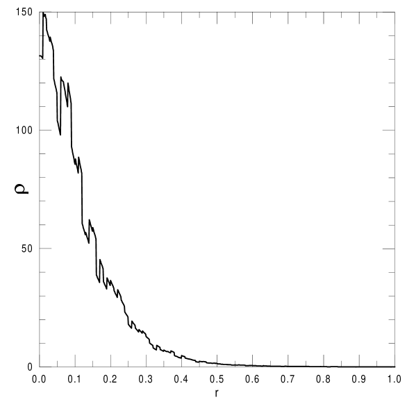
FIG. 1.: Numerical density profile as a fuction of the radial distance for $L_{0}=700$ km and noiselevel $\sqrt{\langle\xi\rangle^{2}}=0.1$.

FIG. 2.: Electron neutrino survival probability for ⁸B neutrinos as a function of $\delta=\Delta m^{2}/(4E)$ for two values of the mixing angle in the SMA region (a) $\sin^{2}(2\theta)=0.006$ and in the LMA region (b) $\sin^{2}(2\theta)=0.78$ and for several values of the correlation length as label in the figure. In both panels the level of noise $\xi=4$%.

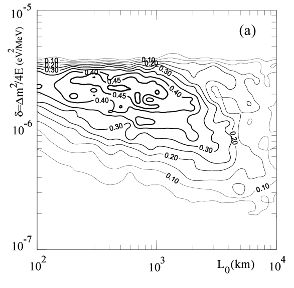
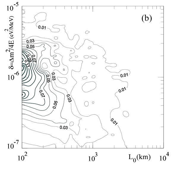
FIG. 3.: Isocontours of constant $[<P_{ee}^{day}(L_{0},\delta)>-P_{ee}^{day}(\delta)]$ values for ⁸B neutrinos in the plane $\delta$, $L_{0}$ for noise level $\xi$ = 4 % and for two values of the mixing angle (a) $s_{2}^{2}=0.0063$ and (b)$s_{2}^{2}=0.79$.

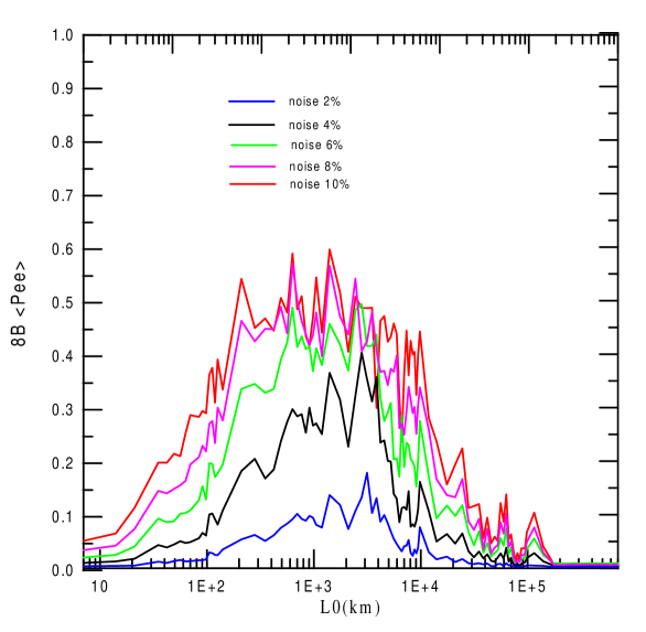
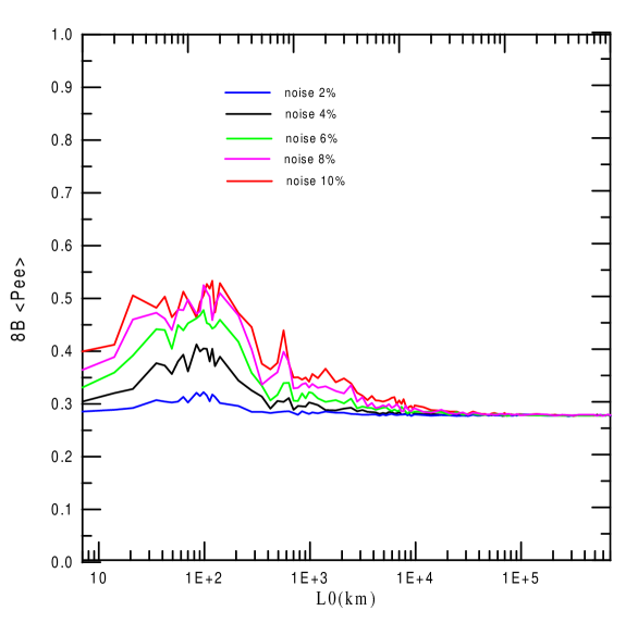
FIG. 4.: Electron neutrino survival probability for ⁸B neutrinos as a function of the correlation length $L_{0}$ for $\delta=3.4\times 10^{-6}$ for two values of the mixing angle (a) $\sin^{2}(2\theta)=0.01$ and (b) $\sin^{2}(2\theta)=0.7$ and for level of noise $\xi=$2 %, %, 8 %, 10 %.

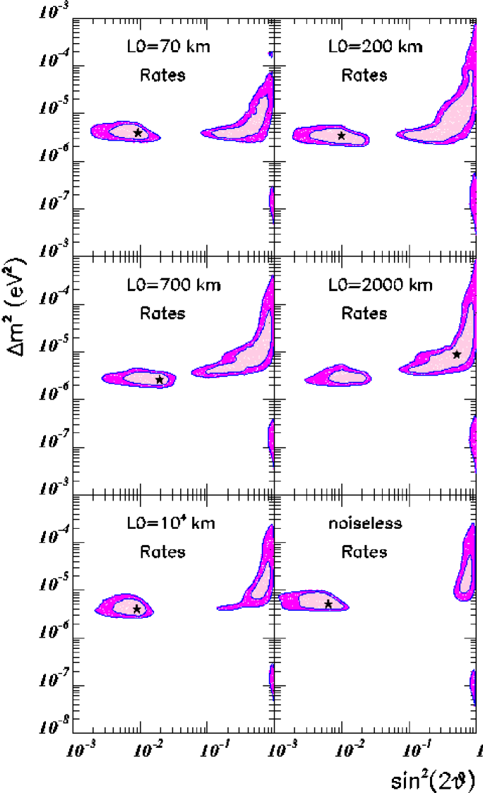
FIG. 5.: Allowed regions in $\Delta m^{2}$ and $\sin^{2}(2\theta)$ from the measurements of the total event rates at Chlorine, Gallium and Super–Kamiokande (825-day data sample) for different correlation lengths and for a noise level $\xi=$4 %. For the sake of comparison the results for the standard noisless analysis is also shown. he darker (lighter) areas indicate the 99% (90%)CL regions. The best–fit point used to defined the regions are indicated by a star.

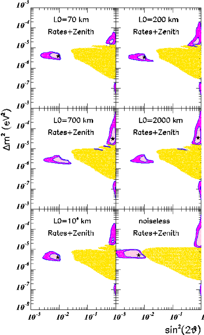
FIG. 6.: Same as Fig. 5 but including also the data on the zenith angle distribution observed in Super–Kamiokande. The shadowed area represents the region excluded by the zenith angle distribution data at 99% CL.

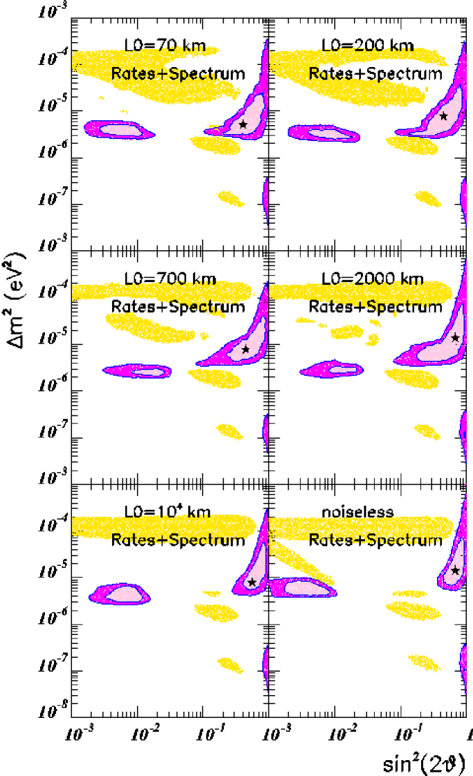
FIG. 7.: Same as Fig. 5 but including also the data on the recoil electron energy spectrum observed in Super–Kamiokande. The shadowed area represents the region excluded by spectrum data at 99% CL.

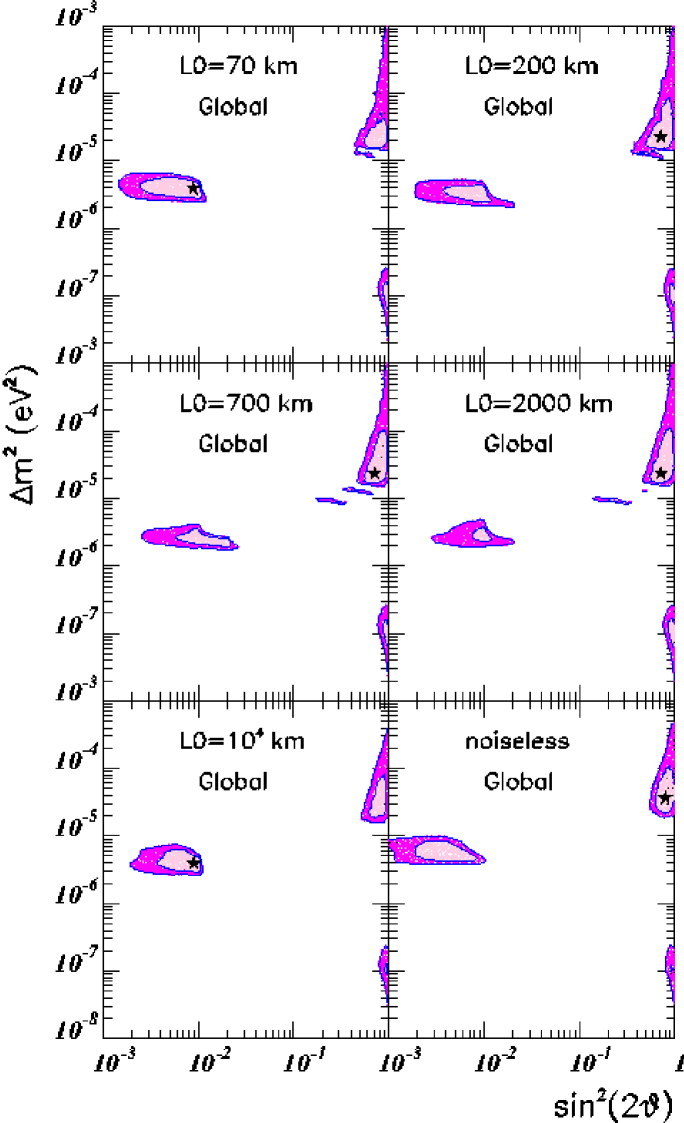
FIG. 8.: Same as Fig. 5 for a global fit to the solar neutrino data.