1. Introduction

Supersymmetric theories now stand as the most promising candidates for a unified theory beyond the standard model [1]. Accurate data remarkably favor the supersymmetric grand unified theory (GUT) over any non-supersymmetric theory [2]. Supersymmetry helps to resolve the gauge hierarchy problem [3]. In non-supersymmetric standard models, because the squared Higgs mass receives a quadratic divergent correction radiatively, we cannot explain the hierarchy between the weak scale and the grand unified scale naturally. Supersymmetry removes the quadratic divergences and provides a framework for naturally explaining the widely separated hierarchy.

Under those contexts, the idea of radiative breaking of the electroweak symmetry [4] is very popular. It is very attractive to explain the breaking of electroweak symmetry through large logarithms between the Planck (or GUT) scale and the weak scale. The radiative corrections drive an up-type Higgs mass-squared parameter negative for a large top Yukawa coupling, and thus the electroweak symmetry breaks down. The radiative symmetry breaking mechanism has consequences for the supersymmetric particle spectrum, and provides important constraints on the particle spectrum.

These constraints also provides a slight puzzle. In the radiative breaking mechanism, the $Z$ boson mass is related to the supersymmetry breaking parameters. We thus believe that supersymmetric particles are not very heavy compared with the $Z$ boson. However, the experimental lower bounds for the supersymmetric particle masses are becoming larger day by day, and it seems that we must require a fine tuning between the parameters in the Higgs potential [5].

It is well known that flavor changing neutral currents (FCNC) make important constraints on the supersymmetry breaking scalar masses [1, 6]. We require that the scalar quark eigenmasses have degeneracy of a few percent when the scalar masses are on the order of O(100) GeV. One solution concerning the scalar quark mass degeneracy is to consider the type of minimal gaugino mediation [7]. Namely, the gaugino mass is almost the only source for supersymmetry breaking at the Planck scale. The supersymmetry breaking parameters which have flavor indices are sufficiently small compared to the gaugino mass at the Planck scale, and become sufficiently large due to renormalization group flow at the low energy scale. Though this scenario is very attractive, such large gaugino masses cause the fine tuning described above to the Higgs potential. Are there any mechanisms in which fine tuning is not required, even if the gaugino mass is large?

In this paper, we insist that the ‘no-scale’ supergravity model [12] does not require any fine tuning of the Higgs potential. The no-scale models are very suitable for the scenario of minimal gaugino mediation. We consider the supersymmetric particle spectrum in no-scale models, where the magnitude of the supersymmetry breaking parameters is also determined radiatively. We can investigate the theoretical upper bounds in no-scale models, and can judge the bounds at near future colliders. Especially, we insist that the no-scale models suggest a natural mass hierarchy between the $Z$ boson mass and the supersymmetry breaking masses.

The organization of this paper is as follows. In Section 2, we review unnatural tuning in the Higgs potential in Minimal Supersymmetric Standard Model (MSSM). In Section 3, we review no-scale supergravity models. In Section 4, we explain how to calculate the particle spectrum in our framework. In Section 5, we show the results for the particle spectrum and discuss its bounds. Finally, we conclude in Section 6 with a summary of our results.

2. Unnatural Tuning in $Z$ Boson Mass

The tree level neutral Higgs potential in MSSM is given by

$$V^{(0)}=m_{1}^{2}|H_{d}^{0}|^{2}+m_{2}^{2}|H_{u}^{0}|^{2}-(m_{3}^{2}H_{d}^{0}H_{u}^{0}+c.c.)+\frac{g^{2}+g^{\prime 2}}{8}(|H_{d}^{0}|^{2}-|H_{u}^{0}|^{2})^{2}.$$ (2.1)

The Higgs mass parameters, $m_{1}^{2}$ and $m_{2}^{2}$, are

$$m_{1}^{2}=m_{H_{d}}^{2}+\mu^{2},\qquad m_{2}^{2}=m_{H_{u}}^{2}+\mu^{2},$$ (2.2)

where $m_{H_{d}}^{2}$ and $m_{H_{u}}^{2}$ are the soft supersymmetry breaking mass squared for the Higgs bosons, and $\mu$ is the so-called Higgsino mass in the supersymmetric ’$\mu$-term’. We denote the vacuum expectation values (VEVs) for $H_{d}^{0}$ and $H_{u}^{0}$ as $v_{d}$ and $v_{u}$, respectively.

We require that electroweak symmetry breaks down, and then find the minimization conditions of the potential at the tree level,

$$\frac{M_{Z}^{2}}{2}=-\mu^{2}+\frac{m_{H_{d}}^{2}-m_{H_{u}}^{2}\tan^{2}\beta}{\tan^{2}\beta-1},$$ (2.3)

$$\sin 2\beta=\frac{2m_{3}^{2}}{m_{1}^{2}+m_{2}^{2}},$$ (2.4)

where $\tan\beta=v_{u}/v_{d}$. We require that the $Z$ boson mass, $M_{Z}$, is equal to 91 GeV and that $\tan\beta$ is not so close at 1, phenomenologically. We should mention here that a relation like Eq.(2.3) is usually satisfied even in non-minimal models.

Radiative electroweak symmetry breaking occurs because $m_{H_{u}}^{2}$ is driven negative due to a large top Yukawa coupling in its renormalization group flow. It is well-known [8] that the heavy gluino mass causes a weird cancellation among supersymmetry breaking Higgs mass squareds and $\mu$ in the $Z$ boson mass formula (2.3).

Let us clarify such an unnatural cancellation. The ‘free’ dimensionful parameters for MSSM is

$$\{m_{0}^{2},M_{1/2},A_{0},B_{0},\mu_{0}\}.$$ (2.5)

These parameters are introduced at the Planck scale. The main contribution for negative $m_{H_{u}}^{2}$ is not the original supersymmetry breaking scalar mass squared $m_{0}^{2}$ at the GUT scale, but the gluino mass, $M_{\tilde{g}}$ [10, 5]. The scalar mass-squared $m_{0}^{2}$ is insensitive to negative $m_{H_{u}}^{2}$ in the regime $m_{0}\sim O(100)$ GeV. Since the most sensitive parameters for the Higgs-mass squared are the gaugino mass, $M_{1/2}$, and $\mu$ among those parameters, the other three parameters are equal to zero for the time being. We show Fig.1 in which we plot the $Z$ boson mass as a function of $\mu/M_{1/2}$ for a given $M_{1/2}$.

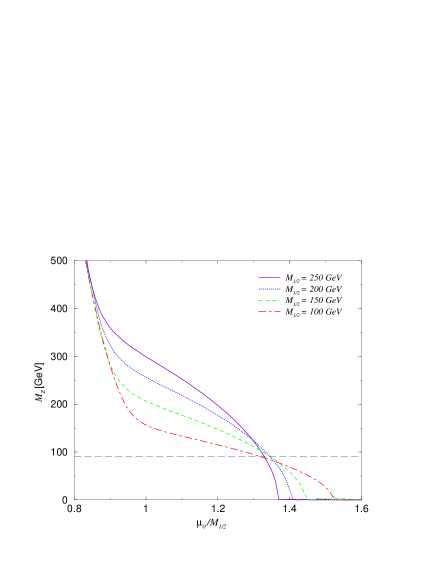
Figure 1: We show the $Z$ boson mass as a function of $\mu_{0}/M_{1/2}$ for various gaugino masses. In this figure, we set $m_{0}$ and $A_{0}$ to be zero. We choose the $B_{0}$ parameter so that $\tan\beta=10$ at the point $M_{Z}=91$ GeV. On the left side of this figure, $\tan\beta$ becomes close to 1, and the Higgs potential is destabilized.

This figure provides us with the problem: why is the parameter $\mu$ limited to within a narrow range for an appropriate electroweak symmetry breaking, even when we solve the $\mu$-problem? Besides, the parameter $\mu$ should be the right edge value in the figure for the allowed region, if the gaugino mass, $M_{1/2}$, is larger than 200 GeV. In fact, $M_{1/2}$ should be larger than about 200 GeV in the minimal gaugino mediation noted in Section 1.

Let us view fine tuning in Eq.(2.3) from another point of view. Here, we suppose that $\tan\beta$ is sufficiently large ($\tan\beta>3$) only for simplicity. Then, the $Z$ boson mass is written by

$$M_{Z}^{2}=-2(\mu^{2}+m_{H_{u}}^{2})=-2m_{2}^{2}.$$ (2.6)

Since parameters $\mu$ and $m_{H_{u}}^{2}$ depend on the scale $Q$, we should know the scale where we require tuning between $\mu^{2}$ and $m_{H_{u}}^{2}$. The scale is the one where 1-loop corrected potential becomes small. We denote the scale as $Q_{\tilde{t}}$, since it is nearly equal to the mass of scalar top quarks. Then, the physical $Z$ boson mass is approximated by

$$M_{Z}^{2}\sim M_{Z}^{2}(Q_{\tilde{t}}),$$ (2.7)

where

$$M_{Z}^{2}(Q)\equiv-2m_{2}^{2}(Q).$$ (2.8)

We define the scale $Q_{0}$ where $M_{Z}^{2}(Q)$ vanish. The $Q_{0}$ is the scale where electroweak symmetry breaks down at the tree level. Expanding $M_{Z}^{2}(Q)$ by $\ln Q$ around scale $Q_{0}$, we obtain

$$M_{Z}^{2}\sim 2\ln(\frac{Q_{0}}{Q_{\tilde{t}}})\frac{dm_{2}^{2}}{d\ln Q}(Q_{0}).$$ (2.9)

From this point of view, the fine tuning in the $Z$ boson mass is translated into the tuning between the scalar quark mass scale $Q_{\tilde{t}}$ and the scale $Q_{0}$. As stated in Ref.[9], electroweak symmetry breaks down only when the scale $Q_{\tilde{t}}$ is less than $Q_{0}$. This fact means the same thing as saying that the parameter $\mu$ should be the right edge in Fig.1 when the gaugino mass becomes greater.

There are many implications about naturalness in the literature. In Ref.[10], it is pointed out that a heavy scalar mass $m_{0}$ (which masses are of the order of 1 TeV) relaxes the fine tuning. Ref.[8] suggests that a less fine-tuned model should be selected as a scenario candidate for supersymmetry breaking. It is preferred that the gaugino mass is not unified at the GUT scale (e.g. D-brane model) in the reference. In this literature, we feel that the fine tuning in the Higgs potential is not dispelled. Are there any models in which cancellation occurs naturally?

In this paper, we suggest that we have already had a model which can explain the heavy gluino mass naturally without any fine tuning. This model is no-scale supergravity. In folklore, it is said that more severe fine tuning is required in the no-scale supergravity model rather than in ordinary models. We believe, however, that this interpretation is not correct. To see this, we give a brief review of no-scale supergravity in the next section.

3. No-Scale Supergravity

In this section, we briefly review the no-scale supergravity, and we consider the natural mass hierarchy between the $Z$ boson and the scalar top in the no-scale model.

In the hidden sector model [11], we separate fields into two sectors, which are a visible sector and a hidden sector. The observable fields (quarks, leptons and Higgs fields) are involved in the visible sector. The hidden fields, which break supersymmetry, exist in the hidden sector, and couple with the observable fields through only gravitational interaction. The $F$ terms of the hidden fields have VEVs due to the dynamics in only the hidden sector in ordinary hidden sector models. In other words, the scale of supersymmetry breaking is determined with no relation to our visible sector. However, it is possible that a scalar potential for the hidden sector fields is flat at the tree level, and that the VEVs of the hidden fields determine radiatively accompanied with visible sector dynamics. Such theories are called no-scale supergravity [12].

Let us see how the gravitino mass is determined in the no-scale model. Using the minimization conditions (2.3) and (2.4), we obtain the tree level MSSM scalar potential at the minimal point,

$$V_{\rm mim}^{(0)}=-\frac{1}{2(g^{2}+g^{\prime 2})}M_{Z}^{4}\cos^{2}2\beta.$$ (3.1)

Since the $Z$ boson mass is proportional to the gravitino mass, the potential involving the hidden sector is unbounded from below. However, there exists a 1-loop corrected scalar potential,

$$V^{(1)}=\frac{1}{64\pi^{2}}\sum_{J}(-1)^{2J}(2J+1)m_{J}^{4}(\ln\frac{m_{J}^{2}}{Q^{2}}-\frac{3}{2}),$$ (3.2)

in $\overline{\rm DR}$ scheme [13]. As a result, the scalar potential is stabilized if Str $M^{4}>0$ [14], and the gravitino mass is determined dynamically.

We emphasize here that the gravitino mass is not independent on the visible sector parameter, namely $\mu$, in the no-scale models. The naturalness argument in the no-scale model differs from arguments in the ordinary ones due to such a dependence.

To confirm the natural hierarchy between the $Z$ boson mass and the supersymmetry breaking masses, we will overview the minimization with respect to gravitino mass [12]. Since the total scalar potential does not depend on the renormalization point, we can evaluate the potential at a scale where the 1-loop corrected potential vanishes,

$$V^{(1)}(v_{u},v_{d};Q)=0.$$ (3.3)

This scale is approximately the mass scale of the scalar top quarks ($Q_{\tilde{t}}$),

$$Q_{\tilde{t}}\equiv(m_{\tilde{t}_{1}}m_{\tilde{t}_{2}})^{1/2}.$$ (3.4)

We can then find the minimal value of the effective scalar potential [12],

$$V_{\rm min}\sim-CQ_{\tilde{t}}^{4}\left(\ln\frac{Q_{\tilde{t}}^{2}}{Q_{0}^{2}}\right)^{2},$$ (3.5)

where $Q_{0}$ is the scale where electroweak symmetry breaks down at the tree level, and $C$ is a constant. In the no-scale model, $Q_{\tilde{t}}$ is determined, by which the $V_{\rm min}$ is minimized. By minimizing $V_{\rm min}$ for $Q_{\tilde{t}}$, we find that the scale $Q_{\tilde{t}}$ is determined as

$$\ln\frac{Q_{0}^{2}}{Q_{\tilde{t}}^{2}}=1.$$ (3.6)

It is important that $Q_{\tilde{t}}$ is very close to $Q_{0}$,

$$Q_{\tilde{t}}=Q_{0}/e^{1/2}.$$ (3.7)

Substituting it into Eq.(2.9), we find the $Z$ boson mass formula in the no-scale model as follows for large $\tan\beta$:

$$M_{Z}^{2}\sim\frac{d}{d\ln Q}m_{2}^{2}.$$ (3.8)

The 1-loop renormalization group equations (RGEs) for $m_{H_{u}}^{2}$ and $\mu^{2}$ are

$$\frac{d}{d\ln Q}m_{H_{u}}^{2}=\frac{1}{2\pi}[3\alpha_{t}(m_{\tilde{t}_{3}}^{2}+m_{\tilde{t}}^{2}+m_{H_{u}}^{2}+A_{t}^{2})-(\alpha^{\prime}M_{1}^{2}+3\alpha_{2}M_{2}^{2})],$$ (3.9)

$$\frac{d}{d\ln Q}\mu^{2}=\frac{1}{2\pi}[3\alpha_{t}+3\alpha_{b}+\alpha_{\tau}-(\alpha^{\prime}+3\alpha_{2})]\mu^{2},$$ (3.10)

where $\alpha_{t}=Y_{t}^{2}/4\pi$ and $Y_{t}$ is a top Yukawa coupling. It turns out that the $Z$ boson mass is determined hierarchically compared to the supersymmetry breaking masses, and that the hierarchy is characterized by 1-loop factor $3\alpha_{t}/2\pi$. This fact is what we insist on in this paper.

Eq.(3.8) is easily extended in the case of a general $\tan\beta$. Expanding Eq.(2.3) by $\ln Q$ around $Q_{0}$, we obtain the following $Z$ boson mass formula at the tree level:

$$M_{Z}^{2}\cos^{2}2\beta\sim\dot{m}_{1}^{2}\cos^{2}\beta+\dot{m}_{2}^{2}\sin^{2}\beta-\dot{m}_{3}^{2}\sin 2\beta,$$ (3.11)

where $\dot{m}_{i}^{2}=dm_{i}^{2}/d\ln Q$. This relation will be tested in the future experiments.

When introducing this formula, we neglect the derivative of the 1-loop corrected potential with respect to Higgs VEVs in the $Z$ boson mass formula. Since it is complicate to write down the derivative, we calculate the 1-loop corrected relation numerically. We show how we obtain our numerical results in the next section.

4. Methods

We concentrate on the following effective scalar potential with a Higgs VEVs independent shift:

$$V_{\rm eff}(v_{u},v_{d})=V^{(0)}(v_{u},v_{d};Q)+V^{(1)}(v_{u},v_{d};Q)-V^{(1)}(v_{u},v_{d}=0;Q).$$ (4.1)

This potential is independent of the renormalization point, $Q$, at the 1-loop level schematically [15]. In the expression, $V^{(0)}$ is a tree level potential (2.1) and $V^{(1)}$ is a 1-loop correction (3.2) of the potential.

At first, we show an effective potential which is minimized by Higgs VEVs $v_{d}$ and $v_{u}$ (Fig.2).

Figure 2: Effective potential Eq.(4.1) minimized by the Higgs vacuum expectation values, $v_{u}$ and $v_{d}$.

This figure is drawn in the minimal case, where $m_{0}^{2}=0$ and $A_{0}=B_{0}=0$. The horizontal axis is for the gaugino mass. We can see that there is a minimum with respect to the gaugino mass.

Since the gaugino mass is the most sensitive parameter for the supersymmetry breaking Higgs mass squared, we normalize the following dimensionful parameters of MSSM:

$$\{m_{0}^{2},M_{1/2},A_{0},B_{0},\mu_{0}\},$$ (4.2)

divided by the gaugino mass $M_{1/2}$, and we adopt the following four dimensionless parameters:

$$\{\hat{m}_{0}^{2},\hat{A}_{0},\hat{B}_{0},\hat{\mu}_{0}\}$$ (4.3)

as parameters for no-scale models. The hat denotes that the parameters are normalized by the gaugino mass (squared). The gaugino mass is determined in minimizing the potential if we fix the hatted parameters. The freedom for $\hat{\mu}_{0}$ is consumed when the $Z$ boson mass is fixed as 91 GeV. If we fix $\tan\beta$, $\hat{B}_{0}$ is consumed and the remaining free parameters are only $\hat{m}_{0}$ and $\hat{A}_{0}$.

To show our numerical analysis, we evolve the supersymmetry breaking parameters with the full two-loop RGEs [16].

Since the potential does not ideally depend on the renormalization point, we may choose any scale. Nevertheless, we minimize the potential (4.1) near to the scale where the electroweak symmetry breaks down at the tree level to fix our aim. This is because we must consider the threshold effect for supersymmetric particles, for instance, scalar quarks and gluinos. Therefore, we adopt our method as follows. Firstly, we minimize the effective potential with respect to the Higgs VEVs and the gaugino mass at the scale above those supersymmetric particle masses. After minimization, we include one-loop threshold corrections from supersymmetric particles [17], and fix the physical quantities. We take as inputs $\alpha_{\rm em}^{-1}(M_{Z})=127.9$, $\sin^{2}\theta_{W}(M_{Z})_{\overline{\rm MS}}=0.2309$ and $M_{Z}=91.2$ GeV.

The strong gauge coupling has a discrepancy between the prediction from GUT and the experimental measurement. The value of the strong gauge coupling, $\alpha_{3}$, is predicted to be $\alpha_{3}(M_{Z})=0.13$ in GUT, while in the experimental measurement, $\alpha_{3}(M_{Z})=0.119$. We adopt the experimental value for the strong gauge coupling. The resulting particle spectra have a great dependence upon the strong gauge coupling and top Yukawa coupling. For smaller gauge coupling, the supersymmetric particles become heavier. This is mainly because the top Yukawa coupling at GUT scale is bigger for the smaller gauge coupling.

We assume that the gaugino masses are unified at the GUT scale. We also assume the universality of $m_{0}^{2}$ and $A_{0}$ for their flavor and matter indices at the GUT scale for simplicity.

In our calculation, the bottom quark mass and the tau lepton mass are fixed as $m_{b}(M_{Z})=3.0$ GeV and $m_{\tau}(M_{Z})=1.7$ GeV. The results we will show later have little dependence on the bottom and tau masses. The top quark pole mass is fixed as $M_{t}=174$ GeV. The 1-loop relationship between the pole mass and tree level mass $Y_{t}v_{u}$ is given by $M_{t}=Y_{t}v_{u}(1+5\alpha_{3}/3\pi)$ in the $\overline{\rm DR}$ scheme.

5. Numerical Results

It is convenient that we present the RGE solution by the following parameterization [5]. The dimensionful parameters at low energy are written using the GUT scale parameters.

First of all, the up-type Higgs mass squared, $m_{2}^{2}$, is written as

$$m_{2}^{2}=1.0\mu_{0}^{2}-0.05m_{0}^{2}-1.75M_{1/2}^{2}-0.34M_{1/2}A_{0}-0.10A_{0}^{2}$$ (5.1)

in the case of $\tan\beta=10$. The mass of the $Z$ boson is $M_{Z}^{2}\sim-2m_{2}^{2}$. It is easy to see that we require fine tuning between $\mu_{0}$ and $M_{1/2}$, if the gaugino is much heavier than $Z$ boson. It is worth noting that the coefficient of $m_{0}^{2}$ is very small in the RGE solution in the expression of $m_{2}^{2}$. This is because the ’focus-point scale’ for $m_{H_{u}}^{2}$ is of the order of 100 GeV [10].

In contrast, the RGE solution for $dm_{2}^{2}/d\ln Q$ is

$$\frac{dm_{2}^{2}}{d\ln Q}=0.015\mu_{0}^{2}+0.026m_{0}^{2}+0.245M_{1/2}^{2}-0.011M_{1/2}A_{0}-0.004A_{0}^{2}$$ (5.2)

when we take $\tan\beta$ = 10. The $Z$ boson mass in the no-scale model is $M_{Z}^{2}\sim dm_{2}^{2}/d\ln Q$. We can easily see that the tuning required above is not necessary in the no-scale model.

Eqs.(5.1) and (5.2) are important for understanding our numerical results qualitatively, such that $-2m_{2}^{2}\sim dm_{2}^{2}/d\ln Q=(100-110{\rm GeV})^{2}$. The numerical value (100-110 GeV) for $M_{Z}$ is caused by the 1-loop corrected potential [18].

We will give the numerical results of minimizing the potential, including the 1-loop corrected potential. In the following figures, the sign of the $\mu$ parameter is positive in the notation used in Eq.(A.4).

In Fig.3, we show a contour plot for the gaugino mass, $M_{1/2}$, as a function of $m_{0}$ and $A_{0}$ in the case of $\tan\beta=10$.

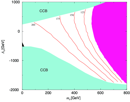
Figure 3: Contour plot for the gaugino mass as a function of $m_{0}$ and $A_{0}$ in the case of $\tan\beta=10$.

The shaded area on the right side of the figure is excluded for the condition $M_{1/2}>100$ GeV, which means that the lightest chargino is heavier than 85 GeV. The upper and lower areas are excluded for charge and color breaking (CCB), namely:

$$A_{t}^{2} > 3(m_{\tilde{q}_{3}}^{2}+m_{\tilde{t}}^{2}+m_{H_{u}}^{2}),$$

$$A_{b}^{2} > 3(m_{\tilde{q}_{3}}^{2}+m_{\tilde{b}}^{2}+m_{H_{d}}^{2}),$$ (5.3)

$$A_{\tau}^{2} > 3(m_{\tilde{\ell}_{3}}^{2}+m_{\tilde{\tau}}^{2}+m_{H_{d}}^{2}).$$

In the black area at $m_{0}\sim 0$ and $A_{0}\sim-500$ GeV, the right-hand scalar tau is lighter than the lightest neutralino, which is not preferred for neutralino LSP. We note that the $m_{0}$ and $A_{0}$ are tuned in the lower right region in the figure. We prefer a small $m_{0}$ because of FCNC constraints. Therefore, we do not regard the large $m_{0}$ region. In Fig.4, we show $m_{0}$-$M_{1/2}$ plot at $A_{0}=0$. We can qualitatively understand its elliptic shape from Eq. (5.2).

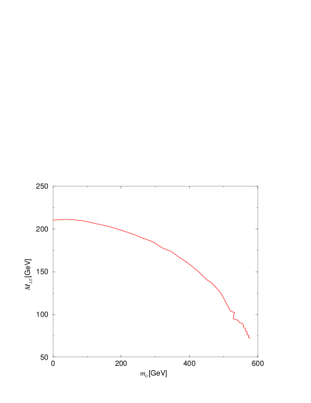
Figure 4: $m_{0}$-$M_{1/2}$ plot at $A_{0}=0$ in the case of $\tan\beta=10$.

Fig.5 shows the chargino masses as a function of $m_{0}$ for various $A_{0}$. We remark that the dots are plotted every 0.2 interval for $\hat{m}_{0}$ (not $m_{0}$), and 0.5 interval for $\hat{A}_{0}$, thus the density of the dots is not related to the probability of the parameters. This remark is also applied in the figure below.

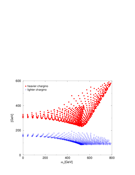
Figure 5: Chargino masses. The heavier and lighter chargino masses are approximately $\mu$ and the wino mass respectively. We cut the lighter chargino mass, which is smaller than 85 GeV.

In Fig.6, we show the gluino mass, lightest chargino mass and lightest neutralino mass as a function of $m_{0}$ for various $A_{0}$ in the same way as in Fig.5.

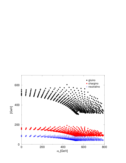
Figure 6: Gluino mass, lightest chargino mass and lightest neutralino mass. The 1-loop correction for gluino mass is included. The lighter chargino mass, which is smaller than 85 GeV, has been cut.

The important prediction for the no-scale model is that the scalar top masses are almost determined independently of the scalar mass, $m_{0}$. The scalar top masses are plotted in Fig.7.

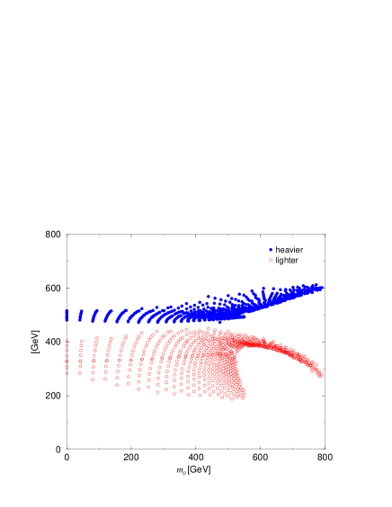
Figure 7: Scalar top masses. The scalar top masses are determined up to left-right mixing.

In supersymmetric models, the lightest Higgs mass is bounded by $M_{Z}$ at the tree level. However, this upper bound is corrected by the 1-loop potential [19]. Since the scalar top masses are almost determined, the lightest Higgs mass is also predictable in the no-scale model. We plot the lightest Higgs mass for $\tan\beta=$ 5, 10, 30 in Fig.8. It is important that the lightest Higgs mass is $110\pm 5$ GeV for small $m_{0}$. The small $m_{0}$ is favored for FCNC constraints. In calculating the lightest Higgs mass, we adopt the 2-loop approximate formula for the mass in Ref.[20].

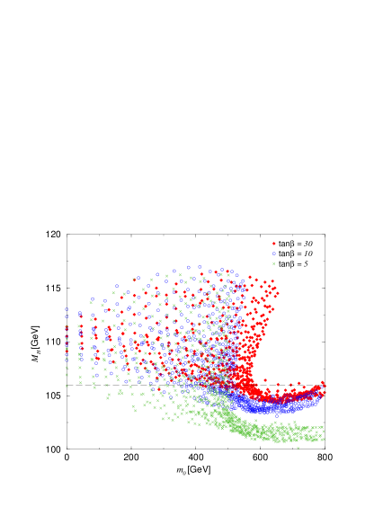
Figure 8: Lightest Higgs mass for $\tan\beta=$ 5,10,30. The dots are plotted every 0.2 interval for $\hat{m}_{0}$ (not $m_{0}$), and 0.5 interval for $\hat{A}_{0}$. The density of the dots is not related to the probability of the parameters. We line the recent LEPII bound on the non-observation of $e^{+}e^{-}\rightarrow ZH$ [21] for one’s information.

6. Discussion

In order to see our insist visibly, we show figure (Fig.9) in the corresponding plot to Fig.1. Again, we set parameter $m_{0}^{2}$ and $A_{0}$ to be zero. We choose the $B_{0}$ parameter so as to be $\tan\beta=$10 at the point $M_{Z}=$91 GeV. We plot the $Z$ boson mass as a function of $\mu_{0}/M_{1/2}(=\hat{\mu}_{0})$. There is no weird constraint for the parameter $\hat{\mu}_{0}$ for electroweak symmetry breaking, contrary to the case in Fig.1. Therefore, the model-building God can create the MSSM parameters without considering whether electroweak symmetry can break down at low energy.

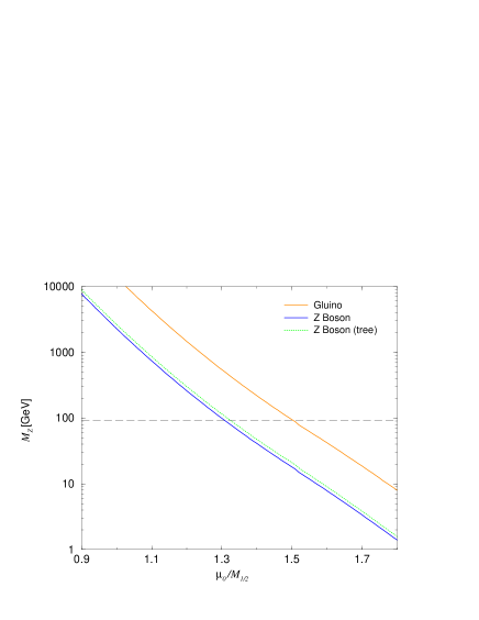
Figure 9: $Z$ boson mass and gluino mass as a function of $\mu_{0}/M_{1/2}$ in the case of the no-scale model. Their mass ratio is approximately constant to $\mu_{0}/M_{1/2}$. We also plot the tree level $Z$ boson mass formula, Eq.(3.8).

Our $Z$ boson mass (91 GeV) does not lie on a special point, contrary to the ordinary case.

The following quantity [22] is usually used for measuring the sensitivity of the $Z$ boson mass for variations in parameter $a$,

$$\Delta_{a}=\left|\frac{\partial\ln M_{Z}^{2}}{\partial\ln a}\right|.$$ (6.1)

The value of $\Delta_{\hat{\mu}_{0}}$ is also large in no-scale model. Namely, the $Z$ boson mass is sensitive to the parameter $\hat{\mu}_{0}$. However, the large value of $\Delta_{\hat{\mu}_{0}}$ in the no-scale model does not cause any fine-tuning problem, contrary to ordinary models. It is just an event that a value of the $Z$ boson mass is selected.

Some people may say that it is also just an event in other supersymmetry breaking scenarios. This opinion is obviously true. However, the predictive ability in the no-scale model is completely different. The subtractive tuning in the ordinary model does not have any predictive power. The supersymmetry breaking mass scale may be of the order of 10 TeV in the ordinary model. On the other hand, we do not require any subtractive tuning in the no-scale model, and predict that all of the supersymmetric particles (except gravitino) appear below about 500-600 GeV. Especially, we can judge the no-scale model when we search the Higgs boson or gauginos in the near future. This predictive ability is our motivation concerning the no-scale model. For theoretical physicists, it is important to search predictive models. To say more, it is important that we recognize that the fine-tuning in the Higgs potential may impose the no-scale supergravity, and we consider predictions of the no-scale models. This is a process of Physics to access the unknown world.

Note added: While completing this paper, we received a paper by R. Barbieri and A. Strumia [23] which also considers that the electroweak breaking scale becomes related to the supersymmetry breaking scale by a loop factor in a similar way to us.

Acknowledgments

Y.M. would like to thank to N. Okada for the discussion of the no-scale supergravity. This work was supported by JSPS Research Fellowships for Young Scientists.

A Notation and Convention

The superpotential of minimal supersymmetric standard model (MSSM) is presented as

$$W=Y_{u}Q\cdot H_{u}U^{c}+Y_{d}H_{d}\cdot QD^{c}+Y_{e}H_{d}\cdot LE^{c}+\mu H_{d}\cdot H_{u},$$ (A.1)

where the SU(2) inner product is defined as

$$H_{d}\cdot H_{u}\equiv H_{d}^{T}\epsilon H_{u},\qquad\epsilon=\left(\begin{array}[]{cc}0&1\\ -1&0\end{array}\right).$$ (A.2)

Here, $Q$, $U^{c}$, $D^{c}$, $L$, $E^{c}$ are matter chiral superfields, and $H_{u}$ and $H_{d}$ are Higgs doublets.

We denote the soft supersymmetry breaking terms as

$$V_{soft} = m_{H_{d}}^{2}|H_{d}|^{2}+m_{H_{u}}^{2}|H_{u}|^{2}$$ (A.3)

$$+m_{\tilde{q}}^{2}\tilde{q}\tilde{q}^{\dagger}+m_{\tilde{u}}^{2}\tilde{u}_{R}\tilde{u}_{R}^{\dagger}+m_{\tilde{d}}^{2}\tilde{d}_{R}\tilde{d}_{R}^{\dagger}+m_{\tilde{\ell}}^{2}\tilde{\ell}\tilde{\ell}^{\dagger}+m_{\tilde{e}}^{2}\tilde{e}_{R}\tilde{e}_{R}^{\dagger}$$

$$+(A_{u}Y_{u}\tilde{q}\cdot H_{u}\tilde{u}_{R}^{c}+A_{d}Y_{d}H_{d}\cdot\tilde{q}\tilde{d}_{R}^{c}+A_{e}Y_{e}H_{d}\cdot\tilde{\ell}\tilde{e}_{R}^{c}+h.c.)$$

$$+(B\mu H_{d}\cdot H_{u}+h.c.)$$

To clarify our notation, we present the left-right component in the scalar top quark mass matrix and chargino mass matrix in the following. The left-right mixing is

$$(A_{t}+\mu\cot\beta)m_{t}.$$ (A.4)

The chargino mass matrix is presented as

$$M_{\chi^{+}}=\left(\begin{array}[]{cc}M_{2}&\sqrt{2}M_{W}\cos\beta\\ \sqrt{2}M_{W}\sin\beta&-\mu\end{array}\right).$$ (A.5)

The supergravity theories are given by the Kähler potential $K$, the superpotential $W$ and the gauge kinetic function $f$. The scalar potential is given in supergravity as

$$V=e^{K}[g^{ij^{*}}(D_{i}W)(D_{j^{*}}W^{*})-3WW^{*}].$$ (A.6)

Using the Kähler transformation $G=K+\log W+\log W^{*}$, we obtain

$$V=e^{G}[G^{i}G_{i}-3].$$ (A.7)

The no-scale Kähler potential [12] is written as

$$G=-3\ln(T+\bar{T}-h(\phi_{i}^{*},\phi_{i}))+\ln|W(\phi_{i})|^{2},$$ (A.8)

where $T$ is a moduli field and $\phi$ are fields in the visible sector. The function $h$ is a Kähler potential for the visible fields. The scalar potential is thus

$$V=\frac{3|W|^{2}}{(T+\bar{T}-h(\phi_{i}^{*},\phi_{i}))^{2}}\left|\frac{\partial W}{\partial\phi_{i}}\right|^{2}.$$ (A.9)

If the global supersymmetric conditions, $\partial W/\partial\phi_{i}=0$, are satisfied, the scalar potential for $T$ is flat and the gravitino mass, $m_{3/2}=e^{G/2}$, is not determined.

Expanding the Kähler potential with respect to visible fields, $Q$, we write the Kähler potential [24] as

$$K=\hat{K}(T,T^{*})+\tilde{K}_{ij^{*}}(T,T^{*})Q^{i}Q^{j^{*}}+\frac{1}{2}(H_{ij}(T,T^{*})Q^{i}Q^{j}+h.c.)+\cdots,$$ (A.10)

where the $T^{\alpha}$’s are hidden sector fields (Dilaton and Moduli). The superpotential is given by

$$W=\hat{W}+\tilde{\mu}_{ij}Q^{i}Q^{j}+\tilde{Y}_{ijk}Q^{i}Q^{j}Q^{k}+\cdots.$$ (A.11)

Substituting VEV into $T$, we obtain the effective superpotential in the flat limit,

$$W_{\rm eff}(Q)=\mu_{ij}Q^{i}Q^{j}+Y_{ijk}Q^{i}Q^{j}Q^{k}.$$ (A.12)

The parameters $\mu$ and $Y$ are written as [24]

$$\mu_{ij}=e^{\hat{K}/2}\frac{\hat{W}^{*}}{|\hat{W}|}\tilde{\mu}_{ij}+m_{3/2}(H_{ij}-G^{\alpha^{*}}\partial_{\alpha^{*}}H_{ij}),$$ (A.13)

$$Y_{ijk}=e^{\hat{K}/2}\frac{\hat{W}^{*}}{|\hat{W}|}\tilde{Y}_{ijk}.$$ (A.14)

In order to solve the $\mu$-problem, we often set $\tilde{\mu}$ to be zero [25]. Then, the $\mu$ parameter in the flat limit is proportional to the gravitino mass.

The gaugino mass is given by the gauge kinetic function, $f_{a}$, as

$$M_{a}=\frac{1}{2}m_{3/2}G^{\alpha}\partial_{\alpha}f_{a}.$$ (A.15)

The supersymmetry breaking scalar mass squared is

$$m^{2}_{ij^{*}}=m_{3/2}^{2}(\tilde{K}_{ij^{*}}-G^{\alpha}G^{\beta^{*}}R_{\alpha\beta^{*}ij^{*}}).$$ (A.16)

Those two parameters are proportional to the gravitino mass (squared).

The $A$ and $B$ parameters are complicated, and are not necessarily proportional to the gravitino mass. In this paper, we suppose that $A$ and $B$ are proportional to the gravitino mass for simplicity.

We note that the parameters $m_{0}$, $A$ and $B$ are zero at the Planck scale in a strict no-scale model, which is given by the Kähler potential (A.8). In this paper, we loosen the boundary condition.

References

- [1] For a review on supersymmetric models, see for instance, H.P. Nilles, Phys. Rev. C110 (1984) 1; H. Haber and G. Kane, Phys. Rev. C117 (1985) 75.
- [2] U. Amaldi, W. de Boer and H. Fürstenau, Phys. Lett. B260 (1991) 445; J. Ellis, S. Kelley and D.V. Nanopoulos, Phys. Lett. B260 (1991) 131.
- [3] S. Dimopoulos and H. Geogi, Nucl. Phys. B193 (1981) 150; N. Sakai, Zeit. f. Phys. C11 (1981) 153; E. Witten, Nucl. Phys. B188 (1981) 513.
- [4] K. Inoue, A. Kakuto, H. Komatsu, and S. Takeshita, Prog. Theor. Phys. 68 (1982) 927; Prog. Theor. Phys. 71 (1984) 413; L. E. Ibáñez, Phys. Lett. 118B (1982) 73; Nucl. Phys. B218 (1983) 514; L. Alvarez-Gaumé, J. Polchinski, and M. Wise, Nucl. Phys. B221 (1983) 495.
- [5] R. Barbieri and G.F. Giudice, Nucl. Phys. B306 (1988) 63.
- [6] S. Dimopoulos and H. Georgi, Nucl. Phys. B193 (1981) 150.
- [7] M. Schmaltz and W. Skiba, hep-ph/0001172; hep-ph/0004210.
- [8] G.L. Kane and S.F. King, Phys. Lett. B451 (1999) 113, M. Bastero-Gil, G.L. Kane and S.F. King, Phys. Lett. B474 (2000) 103.
- [9] G. Gamberini, G. Ridolfi and F. Zwirner, Nucl. Phys. B331 (1990) 331.
- [10] J.L. Feng, K.T. Matchev and T. Moroi, Phys. Rev. D61 (2000) 075005; hep-ph/0003138.
- [11] R. Nath, R. Arnowitt and A. Chamseddine, Phys. Rev. Lett. 49 (1982) 970.
- [12] For a review on no-scale supergravity, A.B. Lahanas and D.V. Nanopoulos, Phys. Rep. 145 (1987) 1.
- [13] S. Coleman and E. Weinberg, Phys. Rev. D7 (1973) 1888.
- [14] C. Kounnas, A. Lahanas, D.V. Nanopoulos and M. Quirós, Nucl. Phys. B236 (1984) 438; J.L. Lopez, D.V. Nanopoulos and K. Yuan, Phys. Rev. D50 (1994) 4060.
- [15] J.A. Casas, V. Di Clemente and M. Quirós, Nucl. Phys. B553 (1999) 511; D.V. Gioutsos, hep-ph/9905278.
- [16] S.P. Martin and M.T. Vaughn, Phys. Rev. D50 (1994) 291; I. Jack and D.R.T. Jones, Phys. Lett. B333 (1994) 372; Y. Yamada, Phys. Rev. D50 (1994) 3537; I. Jack, D.R.T. Jones, S.P. Martin, M.T. Vaughn and Y. Yamada, Phys. Rev. D50 (1994) 5481.
- [17] J. Bagger, K. Matchev and D. Pierce, Phys. Lett. B348 (1995) 443; D. Pierce, J. Bagger, K. Matchev and R.-J. Zhang, Nucl. Phys. B491 (1997) 3.
- [18] R. Arnowitt and P. Nath, Phys. Rev. D46 (1992) 3981.
- [19] Y. Okada, M. Yamaguchi and T. Yanagida, Prog. Theor. Phys. 85 (1991) 1; H.E. Haber and R. Hempfling, Phys. Rev. Lett. 66 (1991) 1815; J. Ellis, G. Ridolfi and F. Zwirner, Phys. Lett. B257 (1991) 83; Phys. Lett. B262 (1991) 477.
- [20] S. Heinemeyer, W. Hollik and G. Weiglein, Phys. Lett. B455 (1999) 179.
- [21] W.J. Marciano, hep-ph/0003181.
- [22] R. Barbieri and G.F. Giudice, Nucl. Phys. B306 (1993) 63.
- [23] R. Barbieri and A. Strumia, hep-ph/0005203.
- [24] V.S. Kaplunovsky and J. Louis, Phys. Lett. B306 (1993) 269.
- [25] G.F. Giudice and A. Masiero, Phys. Lett. B206 (1988) 480.