Constraints on the Mass and Mixing of the 4th Generation Quark From Direct CP Violation $\epsilon^{\prime}/\epsilon$ and Rare $K$ Decays

Abstract

We investigate the $\epsilon^{\prime}/\epsilon$ for $K\rightarrow\pi\pi$ in a sequential fourth generation model. By giving the basic formulae for $\epsilon^{\prime}/\epsilon$ in this model, we analyze the numerical results which are dependent of $m_{t^{\prime}}$ and imaginary part of the fourth CKM factor, $\mbox{Im}V^{*}_{t^{{}^{\prime}}s}V_{t^{{}^{\prime}}d}$ (or $V^{*}_{t^{{}^{\prime}}s}V_{t^{{}^{\prime}}d}$ and the fourth generation CKM matrix phase $\theta$). We find that, unlike the SM, when taking the central values of all parameters for $\epsilon^{\prime}/\epsilon$, the values of $\epsilon^{\prime}/\epsilon$ can easily fit to the current experimental data for all values of hadronic matrix elements estimated from various approaches. Also, we show that the experimental values of $\epsilon^{\prime}/\epsilon$ and rare K decays can provide a strong constraint on both mass and mixing of the fourth generation quark. When taking the values of hadronic matrix elements from the lattice or $1/N$ expansion calculations, a large region of the up-type quark mass $m_{t^{\prime}}$ is excluded.

PACS: 11.30.Er,12.60.-i,13.25.-Es,14.80.-j

1 Introduction

Although the Standard Model (SM) is very successful for explaining the particle physics experiments, it has to face the difficulties of many interesting open questions, such asCP violation. The new experimental results for $\epsilon^{\prime}/\epsilon$, which measures direct CP violation in $K\rightarrow\pi\pi$ decays, have been reported by KTeV collaboration at Fermilab[1] and NA48 collaboration at CERN[2],

$$\mbox{Re}(\epsilon^{\prime}/\epsilon) = (28.0\pm 4.1)\cdot 10^{-4}\qquad{\rm KTeV},$$ (1)

$$\mbox{Re}(\epsilon^{\prime}/\epsilon) = (18.5\pm 7.3)\cdot 10^{-3}\qquad{\rm NA48},$$ (2)

while the new world average reads[2, 3]:

$$\mbox{Re}(\epsilon^{\prime}/\epsilon) = (21.1\pm 4.6)\cdot 10^{-4}$$ (3)

This establishment of direct CP violation rules out old superweak models[4]. Yet while the SM predicts a non-vanishing $\epsilon^{\prime}/\epsilon$, the values in (1), (2) and (3) exceed most theoretical predictions of SM[5, 6]. People have to face and resolve this discrepancy. Some possibilities to accommodate the data in SM have been pointed out [7, 8].

The SM makes precise assumptions on the mechanism that generates the CP violation. The only source of CP violating phase originates from the elements $V_{u_{i}d_{j}}$ of the CKM matrix with three quark generations. In SM, there are both indirect ($\epsilon$) and direct ($\epsilon^{\prime}$) CP violation.The analysis of $\epsilon^{\prime}/\epsilon$ can be divided into the short-distance (perturbative) part and long-distance ( non-perturbative)part. Using the effective Hamiltonian, (${\cal H}_{W}=\sum_{i}C_{i}(\mu)Q_{i}(\mu)$[9, 10]), one can obtain an expression of $\epsilon^{\prime}/\epsilon$ that involves CKM parameters ($V_{u_{i}d_{j}}$), Wilson coefficients ($y_{i}$) and local operator matrix elements ($\langle Q_{i}\rangle_{I}$). The source of most theoretical uncertainties for $\epsilon^{\prime}/\epsilon$ is mainly from the difficulty in calculating non-perturbative part (local operator matrix elements), comparing with the phenomenological determination of CKM parameters [11] and the calculation of the Wilson coefficients at a NLO leval[10]. For $\epsilon^{\prime}/\epsilon$, one of the goals of SM is to determine the hadronic matrix elements[12, 13, 14, 15, 16, 17].

The interesting in this note is not in this non-perturbative part but the new effects with the fourth sequential generation particles in the short-distance part.Except for the SM explanation, there are many directions in the search for New Physics beyond the SM [18, 19, 20, 21, 22, 23, 24] to resolve CP violation. Unlike SM, almost any extension of SM has,in general, new CP violating phases. That is to say, they give new CP violation sources. The new physics on CP violation beyond SM includes CP violation in Supersymmetry models[19] and extensions of fermion sector[20, 23, 24], scalar sector[21] and gauge sector[22] of SM. In extensions of fermion sector, there are many models, such as vector-like quark models[23], sterile neutrino models[24], proposed for probing new effects on CP violation.

In this note, like in ref.[25], we consider a sequential fourth generation model[25, 26], in which an up-type quark $t^{{}^{\prime}}$, adown-type quark $b^{{}^{\prime}}$, a lepton $\tau^{{}^{\prime}}$, and a heavy neutrino $\nu^{{}^{\prime}}$ are added into the SM. The properties of these new fermions are all the same as their corresponding counterparts of other three generations except their masses and CKM mixing, see tab.1,

	up-like quark	down-like quark	charged lepton	neutral lepton
	$u$	$d$	$e$	$\nu_{e}$
SM fermions	$c$	$s$	$\mu$	$\nu_{\mu}$
	$t$	$b$	$\tau$	$\nu_{\tau}$
new fermions	$t^{{}^{\prime}}$	$b^{{}^{\prime}}$	$\tau^{{}^{\prime}}$	$\nu_{\tau^{{}^{\prime}}}$

Table 1: The elementary particle spectrum of SM4

As the SM does not fix the number of generations, so far we don’t know why there is more than one generation and what law of Nature determines their number. On the one hand, the purely sequential 4th generation is constrained, even excluded in many literatures[27]. For example, in refs. [28, 29] the method of Padé approximates is used to show that for a large fermion mass, it is possible to dynamically generate $p$-wave resonance and then the S parameter bound can serve to exclude a heavy fourth generation of fermions[29]. Ref. [30] found that there is no violation of the S parameter upper bound for any value of the heavy fermion mass and that elastic unitarity, imposed as a constraint on strong $W_{L}W_{L}$ scattering, yields no information concerning and sheds no light on the existence of a heavy fourth generation. The ref. [31] compared various precision determinations of the Femi constant $G_{F}$ to get the rather stringent bound of 3rd and 4th generation lepton mixing angle $\theta_{34}$. It founds that the fourth charged lepton is too heavy and seems non-existence. The precision electroweak measurements can also give the strong constrains to the sequential 4th generation, in particlar the S parameter excludes it to 99.8% CL if is degenerate, and if not and a small T parameter is allowed then it is excluded to 98.2% CL [32].

However, on the other hand, experimentally, the LEP determinations of the invisible partial decay width of the $Z^{0}$ gauge boson only show that there are certainly three light neutrinos of the usual type with mass less than $M_{Z}/2$ [33]. But the existence of the fourth generation with a heavy neutrino, i.e., $m_{\nu_{4}}\geq M_{Z}/2$ [34] is not yet excluded. Perhaps there exists some more deep or mechanism to give the room of the sequential fourth generation. Because we really don’t know why there only three generations. So, it is not invalueble to research these new generation as one of the new physics. Before having a more fundamental reason for three generations, one may investigate phenomenologically whether the existing experimental data allow the existence of the fourth generation. This is also the main perpuse of this note. There are a number of papers[26, 27] for discussing the fourth generation phenomena.

In our previous paper[35], we have investigated the constraints on the fourth generation from the inclusive decays of $B\rightarrow X_{s}l^{+}l^{-}$ and $B\rightarrow X_{s}\gamma$. In this note, we further study its effects on direct CP-violating parameter $\epsilon^{\prime}/\epsilon$ in $K\rightarrow\pi\pi$ decays as well as possible new constraints from $\epsilon^{\prime}/\epsilon$ and rare K decays.We limit ourselves to the non-SUSY case in order to concentrate on the phenomenological implication of the fourth generation and will call this model as SM4 hereafter for thesake of simplicity.

CP-violating parameter $\epsilon^{\prime}/\epsilon$ is a short distance dominated process and is sensitive to new physics. In SM4 model, there are not new operators produced. The new particle involved is only the fourth generation up-type quark$t^{\prime}$. The heavy mass of $t^{\prime}$ propagating in the loop diagrams of penguin and box enters the Wilson coefficients $y_{i}$, as well as top quark $t$ and $W$ boson. The effects of the fourth generation particles can only modify $y_{i}$. Each new Wilson coefficients$y^{\rm new}_{i}(\mu)$ is the sum of $y^{\rm sm}_{i}(\mu)$ and $y^{(\rm 4)}_{i}(\mu)$ contributed by t and $t^{\prime}$ correspondingly. We can get $y^{(\rm 4)}_{t^{\prime}}$ by taking the mass of $t^{\prime}$ as one of the input parameter. Moreover, for obtaining $\epsilon^{\prime}/\epsilon$ in SM4,we must know something about elements $V_{{t^{\prime}}d_{j}}$ of the fourth generation $4\times 4$ CKM matrix which now contains nineparemeters, i.e., six angles and three phases.But there are no any direct experimental measurements of them. So we have to get their information indirectly from some meson decays. We investigate three rare $K$ decays, $K^{+}\rightarrow\pi^{+}\nu\bar{\nu}$, $K_{L}\rightarrow\pi^{0}\nu\bar{\nu}$ and $K_{L}\rightarrow\mu^{+}\mu^{-}$[36], in SM4. These decays can give the constraint of the fourth CKM factor, $\mbox{Im}V^{*}_{t^{{}^{\prime}}s}V_{t^{{}^{\prime}}d}$ (or $V^{*}_{t^{{}^{\prime}}s}V_{t^{{}^{\prime}}d}$ and a fourth generation phase $\theta$), which is need for calculating $(\epsilon^{\prime}/\epsilon)^{\rm new}$. We shall take it as an additional input parameter. As a consequence, the total $(\epsilon^{\prime}/\epsilon)$ is the sum of $(\epsilon^{\prime}/\epsilon)^{\rm sm}$ and $(\epsilon^{\prime}/\epsilon)^{\rm 4}$contributed by the SM and the new particle $t^{\prime}$ correspondingly. Unlike the SM, when taking the central values of all parameters for $\epsilon^{\prime}/\epsilon$, the new value of $(\epsilon^{\prime}/\epsilon)$ can reach the range of the current experimental results whatever values of the non-perturbertion part, hadronic matrix elements, are taken in all known cases. Also, the experimental values of $(\epsilon^{\prime}/\epsilon)^{\rm exp}$ impose strong constraints on the parameter space of $\mbox{Im}V^{\ast}_{t^{\prime}s}V_{t^{\prime}d}$and $m_{t^{\prime}}$.

In sec. 2, we give the basic formulae for $\epsilon^{\prime}/\epsilon$ with the fourth up-like quark $t^{\prime}$ in SM4. In sec. 3, we analyze the constraints on the fourth generation CKM matrix factor $\mbox{Im}V^{*}_{t^{{}^{\prime}}s}V_{t^{{}^{\prime}}d}$ which is necessary for calculating$\epsilon^{\prime}/\epsilon$ in SM4. Sec. 4 is devoted to the numerical analysis. Finally, in sec. 5, we give our conclusion.

2 Basic formulae for $\epsilon^{\prime}/\epsilon$ and Wilson Coefficients $y^{(\rm 4)}_{i}(\mu)$ in SM4

The essential theoretical tool for the calculation of $\epsilon^{\prime}/\epsilon$ is the $\Delta S=1$ effective Hamiltonian[9, 10],

$${\cal H}_{W}=\sum_{i}\frac{G_{F}}{\sqrt{2}}V_{ud}\,V^{*}_{us}\Bigl{[}z_{i}(\mu)+\tau\ y_{i}(\mu)\Bigr{]}\;Q_{i}(\mu)\,$$ (4)

with $\tau={V^{*}_{ts}V_{td}}/({V^{*}_{us}V_{ud}})$. The direct CP violation in $K\rightarrow\pi\pi$ is described by $\epsilon^{\prime}$. The parameter $\epsilon^{\prime}$ is given in terms of the amplitudes $A_{0}\equiv A(k\rightarrow(\pi\pi)_{I=0})$ and $A_{2}\equiv A(k\rightarrow(\pi\pi)_{I=2})$ as follows

$$\epsilon^{\prime}=-\frac{1}{\sqrt{2}}\xi(1-\Omega)\exp(i\Phi),$$ (5)

where

$$\xi=\frac{\mbox{Im}A_{0}}{\mbox{Re}A_{0}},\,\omega=\frac{\mbox{Re}A_{2}}{\mbox{Re}A_{0}},\,\Omega=\frac{1}{\omega}\frac{\mbox{Im}A_{2}}{\mbox{Im}A_{0}}$$ (6)

and $\Phi=\pi/2+\delta_{2}-\delta_{0}\approx\pi/4$. With the effective Hamiltonian (4), we can cast (5) into the form

$$\frac{\epsilon^{\prime}}{\epsilon}=\mbox{Im}\lambda_{t}\cdot\left[P^{(1/2)}-P^{(3/2)}\right],$$ (7)

where

$$P^{(1/2)} = \sum P_{i}^{(1/2)}=r\sum y_{i}\langle Q_{i}\rangle_{0}(1-\Omega_{\eta+\eta^{\prime}})$$ (8)

$$P^{(3/2)} = \sum P_{i}^{(3/2)}=\frac{r}{\omega}\sum y_{i}\langle Q_{i}\rangle_{2}.$$ (9)

with $r=G_{F}\omega/(2|\mbox{Re}A_{0})|)$. $y_{i}$ are the Wilson coefficients and the hadronic matrix elements are

$$\langle Q_{i}\rangle_{I}\equiv\langle(\pi\pi)_{I}|Q_{i}|K\rangle$$ (10)

The operators $Q_{i}$ and $\langle Q_{i}\rangle_{I}$ are given explicitly in many reviews[9, 10]

When including the contributions from the fourth generation up-type quark $t^{\prime}$, the above equations will be modified. The corresponding effective Hamiltonian can be expressed as

$${\cal H}_{W}=\sum_{i}\frac{G_{F}}{\sqrt{2}}V_{ud}\,V^{*}_{us}\Bigl{[}z_{i}(\mu)+\tau\ y^{\rm SM}_{i}(\mu)+\tau^{\prime}y^{(\rm 4)}_{i}(\mu)\Bigr{]}\;Q_{i}(\mu)\,.$$ (11)

with $\tau={V^{*}_{ts}V_{td}}$ and $\tau^{\prime}={V^{*}_{t^{{}^{\prime}}s}V_{t^{{}^{\prime}}d}}$. In comparison with the SM, one may introduce the new effective coefficient functions $y^{\rm new}_{i}(\mu)$

$$y^{\rm new}_{i}(\mu)=y^{\rm SM}_{i}+\frac{\tau^{\prime}}{\tau}\cdot y^{(\rm 4)}_{i}(\mu),$$ (12)

where $y_{i}(\mu)$ are the Wilson coefficient functions in the SM and $y_{i}^{(4)}$ are the ones due to fourth generation quark contributions. The evolution for $y^{(\rm 4)}_{i}(\mu)$ is analogy to the one $y^{\rm SM}_{i}(\mu)$ in SM[9, 10] except replacing the t-quark by $t^{\prime}$ quark. The corresponding diagrams of penguin and box are shown in fig. 1.

Using (11) and (12), eq. (7) can be written as

$$(\frac{\epsilon^{\prime}}{\epsilon}) = (\frac{\epsilon^{\prime}}{\epsilon})^{\rm SM}+(\frac{\epsilon^{\prime}}{\epsilon})^{(4)},$$

$$(\frac{\epsilon^{\prime}}{\epsilon})^{(4)} = \mbox{Im}\lambda_{t}^{\prime}\cdot\left[P^{\prime(1/2)}-P^{\prime(3/2)}\right],$$ (13)

where the definitions of $P^{\prime(1/2)}$ and $P^{\prime(3/2)}$ are the same as (8) and (9) only by changing $y_{i}(\mu)$ into $y^{(\rm 4)}_{i}(\mu)$, and

$$\mbox{Im}\lambda_{t^{\prime}}=\mbox{Im}V^{*}_{t^{{}^{\prime}}s}V_{t^{{}^{\prime}}d}.$$ (14)

Thus the main test of evaluating $\epsilon^{\prime}/\epsilon$ in the SM4 is to calculate the Wilson coefficients $y^{(\rm 4)}_{i}(\mu)$ and to provide the possible constraints on $\mbox{Im}\lambda_{t^{\prime}}$. The constraints of $\mbox{Im}\lambda_{t^{\prime}}$ will be discussed in next section. The calculation of $y^{(\rm 4)}_{i}(\mu)$ is the same as their counterpart $y^{\rm SM}_{i}(\mu)$ in SM and can be simply done by changing $m_{t}$ to $m_{t^{{}^{\prime}}}$, which is easy to be found in any corresponding reviews[9, 10]. Here we repeat the same calculations and only provide the numerical results for $y^{(\rm 4)}_{i}(\mu)$ as the functions of the mass $m_{t}^{{}^{\prime}}$. In the numerical calculations we take a large range for $t^{{}^{\prime}}$-quark mass $m_{t^{\prime}}=$ 50GeV, 100GeV, 150GeV, 200GeV, 250GeV, 300GeV, 400Gev [26] See tab. 2,

$m_{t}^{{}^{\prime}}$(GeV)	50	100	150	200	250	300	350	400
$z_{1}^{\rm 4}$	-0.594	-0.594	-0.594	-0.594	-0.594	-0.594	-0.594	-0.594
$z_{2}^{\rm 4}$	0.323	0.323	0.323	0.323	0.323	0.323	0.323	0.323
$y_{3}^{\rm 4}$	0.028	0.032	0.036	0.042	0.048	0.055	0.064	0.074
$y_{4}^{\rm 4}$	-0.049	-0.052	-0.056	-0.059	-0.064	-0.069	-0.075	-0.081
$y_{5}^{\rm 4}$	0.011	0.011	0.012	0.012	0.013	0.013	0.014	0.014
$y_{6}^{\rm 4}$	-0.089	-0.097	-0.112	-0.104	-0.107	-0.111	-0.114	-0.118
$y_{7}^{\rm 4}/\alpha$	-0.114	-0.076	-0.004	0.092	0.210	0.348	0.506	0.686
$y_{8}^{\rm 4}/\alpha$	-0.034	0.011	0.097	0.210	0.350	0.514	0.704	0.917
$y_{9}^{\rm 4}/\alpha$	-0.367	-0.825	-1.335	-1.913	-2.571	-3.318	-4.159	-5.098
$y_{10}^{\rm 4}/\alpha$	0.172	0.397	0.6475	0.932	1.255	1.622	2.037	2.498

Table 2: $\Delta S=1$ Wilson coefficients at $\mu=1.0{\rm GeV}$ for $\Lambda^{(\rm 4)}=340{\rm MeV}$ and $f=3$ effective flavors at leading order. $y_{1}^{\rm 4}=y_{2}^{\rm 4}\equiv 0$.

3 Constraints on CKM Factor $V^{*}_{t^{{}^{\prime}}s}V_{t^{{}^{\prime}}d}$ in SM4

Though we have no direct information for the additional fourth generation CKM matrix elements, while constraints may be obtained from some rare meson decays. In ref.[35], we obtained the values of the fourth CKM factor $V^{*}_{t^{{}^{\prime}}s}V_{t^{{}^{\prime}}b}$ from the decay of $B\rightarrow s\gamma$. In this paper, we shall investigate three rare $K$ meson decays: two semi-leptonic decays $K^{+}\rightarrow\pi^{+}\nu\bar{\nu}$ and $K_{L}\rightarrow\pi^{0}\nu\bar{\nu}$, and one leptonic decay $K_{L}\rightarrow\mu^{+}\mu^{-}$[36] within SM4. These decays can provide certain constraints on the fourth generation CKM factors, $V^{*}_{t^{{}^{\prime}}s}V_{t^{{}^{\prime}}d}$ , $\mbox{Im}V^{*}_{t^{{}^{\prime}}s}V_{t^{{}^{\prime}}d}$ and $\mbox{Re}V^{*}_{t^{{}^{\prime}}s}V_{t^{{}^{\prime}}d}$ respectively.

Within SM, the decays $K\rightarrow\pi\nu\bar{\nu}$ are loop-induced semileptonic FCNC process determined only by $Z^{0}$-penguin and box diagram. These decays are the theoretically cleanest decays in rare K-decays. The great virtue of $K_{L}\rightarrow\pi^{0}\nu\bar{\nu}$ is that it proceeds almost exclusively through direct CP violation [45] which is very important for the investigation of $\epsilon^{{}^{\prime}}/\epsilon$ in SM4. The precise calculation of these two decays at the NLO in SM can be found in Refs[46]. While experimentally, its branching ratio has not yet been well measured, only an upper bound has be given and is larger by one order of magnitude than the one in SM (see tab. 3). This remains allowing the New Physics to dominate their decay amplitude[18]. Moreover, Unlike the previous two semi-leptonic decays, the branching ratio $Br(K_{L}\rightarrow\mu^{+}\mu^{-})$ has already been measured with a very good precision. While its experimental result is several times larger than theoretical prediction in SM (see tab. 3). This also provides a window for New Physics.

	$Br(K^{+}\to\pi^{+}\nu\bar{\nu})$	$Br(K_{L}\to\pi^{0}\nu\bar{\nu})$	$Br(K_{L}\rightarrow\mu^{+}\mu^{-}$)
Experiment	$<2.4\times 10^{-9}$[37]	$<1.6\times 10^{-6}$[38]	$(6.9\pm 0.4)\times 10^{-9}$[39]
	$(4.2+9.7-3.5)\times 10^{-10}$[44]	$<6.1\times 10^{-9}$[40]	$(7.9\pm 0.7)\times 10^{-9}$[41]
SM	$(8.2\pm 3.2)\times 10^{-11}$[43]	$(3.1\pm 1.3)\times 10^{-11}$ [43]	$(1.3\pm 0.6)\times 10^{-9}$[42]

Table 3: Comparison of $B(K^{+}\to\pi^{+}\nu\bar{\nu})$, $B(K_{L}\to\pi^{0}\nu\bar{\nu})$ and $B(K_{L}\to\pi^{0}\nu\bar{\nu})$ among the experimental values and SM predictions with maximum mixing.

In the SM4, the branching ratios of the three decay modes mentioned above receive additional contributions from the up-type quark $t^{\prime}$ [47]

$$Br(K^{+}\to\pi^{+}\nu\bar{\nu})=\kappa_{+}\left|\frac{V_{cd}V_{cs}^{*}}{\lambda}P_{0}+\frac{V_{td}V_{ts}^{*}}{\lambda^{5}}\eta_{t}X_{0}(x_{t})+\frac{V_{t^{\prime}d}V_{t^{\prime}s}^{*}}{\lambda^{5}}\eta_{t^{\prime}}X_{0}(x_{t^{\prime}})\right|^{2},$$ (15)

$$Br(K_{L}\to\pi^{0}\nu\bar{\nu})=\kappa_{L}\left|\frac{{\rm Im}V_{td}V_{ts}^{*}}{\lambda^{5}}\eta_{t}X_{0}(x_{t})+\frac{{\rm Im}V_{t^{\prime}d}V_{t^{\prime}s}^{*}}{\lambda^{5}}\eta_{t^{\prime}}X_{0}(x_{t^{\prime}})\right|^{2},$$ (16)

$$Br(K_{L}\to\mu\bar{\mu})_{\rm SD}=\kappa_{\mu}\left[\frac{{\rm Re}\left(V_{cd}V_{cs}^{*}\right)}{\lambda}P^{\prime}_{0}+\frac{{\rm Re}\left(V_{td}V_{ts}^{*}\right)}{\lambda^{5}}Y_{0}(x_{t})+\frac{{\rm Re}\left(V_{t^{\prime}d}V_{t^{\prime}s}^{*}\right)}{\lambda^{5}}Y_{0}(x_{t^{\prime}})\right]^{2}.$$ (17)

where $\kappa_{+},\kappa_{L},\kappa_{\mu}$,$X_{0}(x_{t})$ , $X_{0}(x_{t^{\prime}})$, $Y_{0}(x_{t})$ ,$Y_{0}(x_{t^{\prime}})$,$P_{0},P^{\prime}_{0}$ may be found in Refs[9, 10]. The QCD correction factors are taken to be $\eta_{t}=$ 0.985 and $\eta_{t^{\prime}}=$ 1.0 [47].

To solve the constrains of the 4th generation CKM matrix factors $V^{*}_{t^{{}^{\prime}}s}V_{t^{{}^{\prime}}d}$, ${\rm Im}V^{*}_{t^{{}^{\prime}}s}V_{t^{{}^{\prime}}d}$ and ${\rm Re}V^{*}_{t^{{}^{\prime}}s}V_{t^{{}^{\prime}}d}$, we must conculate the Wilson coefficients $X_{0}(x_{t^{\prime}})$ and $Y_{0}(x_{t^{\prime}})$. They are the founctions of the mass of the 4th generation top quark, $m_{t^{\prime}}$. Here we give their numerical results according to several values of $m_{t^{\prime}}$, (see table 4)

$m_{t^{\prime}}$(GeV)	50	100	150	200	250	300	400	500	600
$X_{0}(x_{t^{\prime}})$	0.404	0.873	1.357	1.884	2.474	3.137	4.703	6.615	8.887
$Y_{0}(x_{t^{\prime}})$	0.144	0.443	0.833	1.303	1.856	2.499	4.027	5.919	8.179

Table 4: Wilson coefficients $X_{0}(x_{t^{\prime}})$, $Y_{0}(x_{t^{\prime}})$ to $m_{t^{\prime}}$

We found that the Wilson coefficients $X_{0}(x_{t^{\prime}})$ and $Y_{0}(x_{t^{\prime}})$ increase with the $m_{t^{\prime}}$. To get the largest constrain of the factors in eq. (15), (16) and (17), we must use the little value of $m_{t^{\prime}}$. Considering that the 4th generation particles must have the mass larger than $M_{Z}/2$ [33], we take $m_{t^{\prime}}$ with 50 GeV to get our constrains of those three factors.

Then, from (15), (16) and (17), we arrive at the following constraints

$$|V^{*}_{t^{{}^{\prime}}s}V_{t^{{}^{\prime}}d}|\leq 2\times 10^{-4},$$ (18)

$$|\mbox{Im}V^{*}_{t^{{}^{\prime}}s}V_{t^{{}^{\prime}}d}|\leq 1.2\times 10^{-4},$$ (19)

$$|\mbox{Re}V^{*}_{t^{{}^{\prime}}s}V_{t^{{}^{\prime}}d}|\leq 1.0\times 10^{-4}.$$ (20)

For the numerical calculations, we will take $|\mbox{Im}V^{*}_{t^{{}^{\prime}}s}V_{t^{{}^{\prime}}d}|\leq 1.2\times 10^{-4}$.

It is easy to check that the equation (18) obeys the CKM matrix unitarity constraint, which states that any pair of rows, or any pair of columns, of the CKM matrix are orthogonal.[11]. The relevant one to those decay channels is

$$V_{us}^{*}V_{ud}+V_{cs}^{*}V_{cd}+V_{ts}^{*}V_{td}+V_{t^{{}^{\prime}}s}^{*}V_{t^{{}^{\prime}}d}=0.$$ (21)

Here we have taken the average values of the SM CKM matrix elements from Ref. [11]. Considering the fact that the data of CKM matrix is not yet very accurate, there still exists a sizable error for the sum of the first three terms. Using the value of $V^{*}_{t^{{}^{\prime}}s}V_{t^{{}^{\prime}}d}$ obtained from eq. (18), the sum of the four terms in the left hand of (21) can still be close to $0$, because the values of $V^{*}_{t^{{}^{\prime}}s}V_{t^{{}^{\prime}}d}$ are about $10^{-4}$ order, ten times smaller than the sum of the first three ones in the left of (21). Thus, the values of $V^{*}_{t^{{}^{\prime}}s}V_{t^{{}^{\prime}}d}$ remain satisfying the CKM matrix unitarity constraints in SM4 within the present uncertainties.

4 The Numerical Analysis

In the calculation of $\epsilon^{\prime}/\epsilon$, the main source of uncertainty are the hadronic matrix elements $\langle Q_{i}\rangle_{I}$. They depend generally on the renormalization scale $\mu$ and on the scheme used to renormlize the operators $Q_{i}$. But the calculation of $\langle Q_{i}\rangle_{I}$ is much beyond the perturbative method. They only can be tread by the non-perturbative methods, like lattice methods, $1/N$ expansion, chiral quark models and chiral effective langrangians, which is not sufficient to obtain the high accuracy. We shall present the analysis on $t^{{}^{\prime}}$-quark effects when considering the uncertainties of $\langle Q_{i}\rangle_{I}$ due to model-dependent calculations.

It is customary to express the matrix elements $\langle Q_{i}\rangle_{I}$ in terms of non-perturbative parameters $B^{\rm(1/2)}_{i}$ and $B^{\rm(3/2)}_{i}$ as follows:

$$\langle Q_{i}\rangle_{0}\equiv B^{\rm(1/2)}_{i}\langle Q_{i}\rangle^{(\rm vac)}_{0};\langle Q_{i}\rangle_{2}\equiv B^{\rm(3/2)}_{i}\langle Q_{i}\rangle^{(\rm vac)}_{2}.$$ (22)

The full list of $\langle Q_{i}\rangle_{I}$ is given in ref.[12]. We take the phenomenological values of $B_{i}$[17] (see tab.5) except for $B^{(1/2)}_{6}$ and $B^{(3/2)}_{8}$ which are taken as input parameter with values calculated by three different non-perturbative methods. Other numerical input parameters are given in tab.6.

$B_{1}^{\rm(1/2)}$	$B_{2}^{\rm(1/2)}$	$B_{3}^{\rm(1/2)}$	$B_{4}^{\rm(1/2)}$	$B_{5}^{\rm(1/2)}$	${\bf B_{6}^{\bf(1/2)}}$	$B_{7}^{\rm(1/2)}$	$B_{8}^{\rm(1/2)}$	$B_{9}^{\rm(1/2)}$	$B_{10}^{\rm(1/2)}$
$13.0$	$6.1\pm 1.0$	$1.0^{*}$	$5.2^{*}$	$B_{6}^{\rm(1/2)}$	INPUT	$1.0^{*}$	$1.0^{*}$	$7.0^{*}$	$7.5^{*}$
$B_{1}^{\rm(3/2)}$	$B_{2}^{\rm(3/2)}$	$B_{3}^{\rm(3/2)}$	$B_{4}^{\rm(3/2)}$	$B_{5}^{\rm(3/2)}$	$B_{6}^{\rm(3/2)}$	$B_{7}^{\rm(3/2)}$	${\bf B_{8}^{\bf(3/2)}}$	$B_{9}^{\rm(3/2)}$	$B_{10}^{\rm(3/2)}$
$0.48$	$0.48$	$1.0^{*}$	$5.2^{*}$	$1.0\pm 0.3^{*}$	$1.0\pm 0.3^{*}$	$1.0^{*}$	INPUT	$0.48$	$0.48$

Table 5: Phenomennolegical values of $B_{i}$. ^∗ stands for an ”educated guess”.

$\mbox{Re}A_{0}$	$3.33\times 10^{-7}$GeV	$\Omega_{\eta\eta^{{}^{\prime}}}$	$0.25$	$G_{\rm F}$	$1.166\times 10^{-5}$GeV-2
$\mbox{Re}A_{2}$	$1.50\times 10^{-8}$GeV	$\omega$	$0.045$	$\mbox{Im}\lambda_{t}$	$1.34\times 10^{-4}$
$m_{d}(m_{c})$	$8$MeV	$m_{\pi}$	$138$MeV	$\Lambda^{\rm 4}_{\rm\overline{MS}}$	3$40$MeV
$m_{s}(m_{c})$	$130$GeV	$m_{\rm K}$	$498$MeV	$M_{W}$	$80.2$GeV
$m_{c}(m_{c})$	$1.3$GeV	$F_{\pi}$	$131$MeV	$\alpha_{s}(M_{Z})$	$0.117$
$m_{b}(m_{b})$	$4.8$GeV	$F_{\rm K}$	$160$MeV	$\alpha$	$1/129$
$m_{t}(m_{t})$	$175$GeV			$\sin\theta_{W}$	$0.23$

Table 6: Neumerical values of the input parameters.

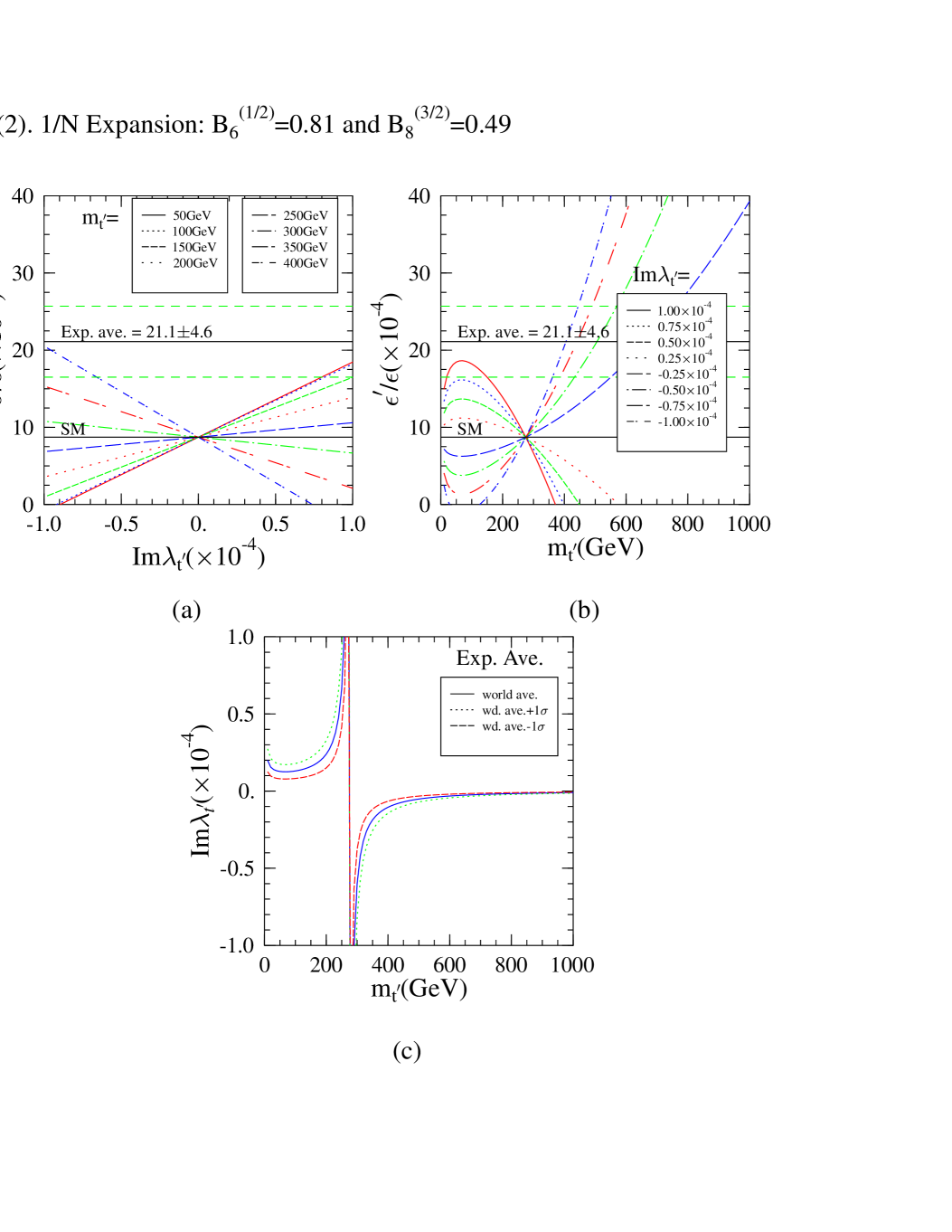
Figure 3: Same as fig. 1 in $1/N$ Expansion.

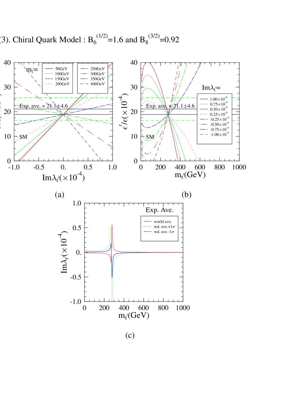
Figure 4: Same as fig. 1 in Chiral Quark Model.

We take the values of $B_{6}^{\rm(1/2)}$and $B_{8}^{\rm(3/2)}$ in three non-perturbitive approaches, lattice methods, $1/N$ expansion and chiral quark models (see tab.7) and the figs (see figs.2, 3, 4) in each case respectively.

	lattice method	$1/N$ expansion	chiral quark models
$B_{6}^{\rm(1/2)}$	$1.0\pm 0.02\pm 0.05$[48]	$0.81$[6]	$1.6\pm 0.3$[7]
$B_{8}^{\rm(3/2)}$	$0.8\pm 0.15$[14]	$0.49$[6]	$0.92\pm 0.002$[7]

Table 7: The input values of $B_{6}^{\rm(1/2)}$ and $B_{8}^{\rm(3/2)}$ in three cases.

The numerical results are shown in figs. 2,3,4 which correspond to the three cases of calculating hadronic matrix elements, lattice method, 1/N eapansion, and chiral quark model, respectively. We now present a study for $\epsilon^{{}^{\prime}}/\epsilon$ as functions of $\mbox{Im}\lambda_{t^{\prime}}$ and $m_{t^{\prime}}$: $\epsilon^{{}^{\prime}}/\epsilon$ versus $\mbox{Im}\lambda_{t^{\prime}}$ with fixing $m_{t^{{}^{\prime}}}$ is plotted in figs. (a); $\epsilon^{{}^{\prime}}/\epsilon$ versus $m_{t^{\prime}}$ with fixing $\mbox{Im}\lambda_{t^{\prime}}$ is ploted in figs. (b); and the allowed parameter space of $\mbox{Im}\lambda_{t^{\prime}}$ and $m_{t^{{}^{\prime}}}$ is plotted in figs. (c). We shall analyze each case in detail as follows.

In figs (a) we plot eight lines corresponding to $m_{t^{{}^{\prime}}}=$50, 100, 150, 200 250, 300, 350, 400GeV respectively. First, we notice that the slope of the line decreases as $m_{t^{{}^{\prime}}}$ increases. At a value of $m_{t^{{}^{\prime}}}$, about 230GeV, the slope is zero because the second part in the right hand side of eq. (13) vanishes. The reason is similar to that in SM, i.e., with increasing $m_{t^{{}^{\prime}}}$ the EW penguins become increasingly important and their contributions to $\epsilon^{{}^{\prime}}/\epsilon$ are with the opposite sign to those of QCD penguins so that at some values of $m_{t^{{}^{\prime}}}$ there is a cancellation. The behavior comes essentially once $m_{t^{{}^{\prime}}}$ becomes larger than 230GeV, the slope is negative. Its absolute value increases with $m_{t^{{}^{\prime}}}$. Such a behavior comes essentially from the change of the Wilson coefficients $y_{i}^{(\rm 4)}$ as $m_{t^{{}^{\prime}}}$. Second, from figs (a), we found, within the constraints on $\mbox{Im}\lambda_{t^{\prime}}$ from the three rare $K$ meson decays, that $\epsilon^{{}^{\prime}}/\epsilon$ can generally be consistent with the experimental average except for some ranges of $m_{t^{{}^{\prime}}}$ once the non-perturbative parameters $B_{6}^{\rm(1/2)}$ and $B_{8}^{\rm(3/2)}$ are taken values calculated based on the lattice gauge theory and $1/N$ expansion. Such a range roughly ranges from 170GeV to 300GeV, which can be seen from figs. (2a) and (3a). There is no excluded range for the case of the chiral quark model. This is because in the first two cases, the SM values $(\epsilon^{{}^{\prime}}/\epsilon)^{\rm SM}$ are about $8.8\times 10^{-4}$, which is much lower than the experimental average. For a large range of $m_{t^{{}^{\prime}}}$, $(\epsilon^{{}^{\prime}}/\epsilon)^{(4)}$ is not large enough to make total $\epsilon^{{}^{\prime}}/\epsilon$ reach the experimental average. But in the chiral quark model, the SM value is about $18.8\times 10^{-4}$ which is in the $1\sigma$ error range of the present experimental average so that $\epsilon^{{}^{\prime}}/\epsilon$ can reach the experimental average for all values of $m_{t^{{}^{\prime}}}$ in the reasonable region. Thus once the non-perturbative method calculations become more reliable and the experimental measurements get more accuracy, it may provide more strong constraints on the forth generation quark from the study on $\epsilon^{{}^{\prime}}/\epsilon$. Unfortunately, we can’t get any information on the upper bound of $m_{t^{{}^{\prime}}}$.

We also plot in Figs (b) eight curves corresponding to $\mbox{Im}\lambda_{t^{\prime}}=$1.0, 0.75, 0.5, 0.25, -0.25, -0.5, -0.75, -1.0$\times 10^{-4}$ respectively. Thus similar results as those in the figs (a) are arrived. These curves are divided into two types determined by the sign of the fourth generation CKM factor $\mbox{Im}\lambda_{t^{\prime}}$. The reason is also similar to the analysis for figs. (a). The figs.(b) also show the constraints on $\mbox{Im}\lambda_{t^{\prime}}$. It is interesting to see that there is an excluded region from 0 to $0.6\times 10^{-4}$ based on lattice gauge theory results and from 0 to $0.76\times 10^{-4}$ based on the $1/N$ expansion results. While there is no such an excluded region based on the chiral quark model results. The reason is the same as that in the analysis of figs (a). Moreover, it seems that $\mbox{Im}\lambda_{t^{\prime}}$ favors the negative values which may be interesting since the negative value of $\mbox{Im}\lambda_{t^{\prime}}$ is better to satisfy the unitarity constraints of the CKM matrix (see eq. (21)). Therefore if there could exist the fourth generation, from both the theoretical and the experimental parts, one might be able get usefull information on the fourth generation CKM matrix elements, such as $V^{*}_{t^{{}^{\prime}}s}V_{t^{{}^{\prime}}b}$ which has been studied in our previous paper[35].

In figs. (c), we show the correlation between $\mbox{Im}\lambda_{t^{\prime}}$ and $m_{t^{{}^{\prime}}}$. The three curves in the figure correspond to the experimental values of the new world average and its $1\sigma$ error, respectively. It is seen that the the allowed parameter space is strongly limited for all three cases when the ratio $\epsilon^{{}^{\prime}}/\epsilon$ is around the present experimental average within 1 $\sigma$ error. The allowed parameter space is divided into two pieces except in the chiral quark model. This is in agreement with the analyses in figs. (a) and (b). Such a small parameter space indicates that $\epsilon^{{}^{\prime}}/\epsilon$ may impose a very strong constraint on the mass and mixing of the fourth generation up-type quark.

5 Conclusion

In summary, we have investigated the direct CP-violating parameter $\epsilon^{\prime}/\epsilon$ in $K^{0}-\bar{K}^{0}$ system with considering the up-type quark $t^{\prime}$ in SM4. The basic formulae for $\epsilon^{\prime}/\epsilon$ in SM4 has been presented and the Wilson coefficient functions in the SM4 have also been evaluated. The numerical results of the additional Wilson coefficient functions have been given as functions of the mass $m_{t^{\prime}}$. We have also studied the relevant rare $K$ meson decays: two semi-leptonic decays, $K^{+}\rightarrow\pi^{+}\nu\bar{\nu}$ and $K_{L}\rightarrow\pi^{0}\nu\bar{\nu}$, and one leptionic decay $K_{L}\rightarrow\mu^{+}\mu^{-}$, which allow us to obtain the bounds on the fourth generation CKM matrix factor $V^{*}_{t^{{}^{\prime}}s}V_{t^{{}^{\prime}}d}$. In particular, we have analyzed the numerical result of $\epsilon^{\prime}/\epsilon$ as the function of $m_{t^{\prime}}$ and imaginary part of the fourth CKM factor, $\mbox{Im}V^{*}_{t^{{}^{\prime}}s}V_{t^{{}^{\prime}}d}$ (or $V^{*}_{t^{{}^{\prime}}s}V_{t^{{}^{\prime}}d}$ and a fourth generation CKM matrix phase $\theta$). The correlation between $\epsilon^{\prime}/\epsilon$ and $\mbox{Im}V^{*}_{t^{{}^{\prime}}s}V_{t^{{}^{\prime}}d}$ has been studied in detail with different hadronic matrix elements calculated from various approaches, such as lattice gauge method, $1/N$ expansion and chiral quark model. It has been seen that, unlike the SM, when taking the central values of all parameters, the values of $\epsilon^{\prime}/\epsilon$ can be easily made to be consistent with the current experimental data for all estimated values of the relevant hadronic matrix elements from various approaches. Especially, we have also investigated the allowed parameter space of $m_{t^{{}^{\prime}}}$ and $\mbox{Im}V^{*}_{t^{{}^{\prime}}s}V_{t^{{}^{\prime}}d}$, as a consequence, when considering $1\sigma$-error of the current experimental data for $\epsilon^{\prime}/\epsilon$, the allowed parameter space for $m_{t^{{}^{\prime}}}$ and $\mbox{Im}V^{*}_{t^{{}^{\prime}}s}V_{t^{{}^{\prime}}d}$ is very small and strongly restricted. This implies that the experimental data in K system can provide strong constraints on the mass of $t^{\prime}$-quark and also on the fourth generation quark mixing matrix.

Figure 1: The Additional Diagrams of (a) EW, (b) QCD Penguins and (b) Box with $t^{{}^{\prime}}$.

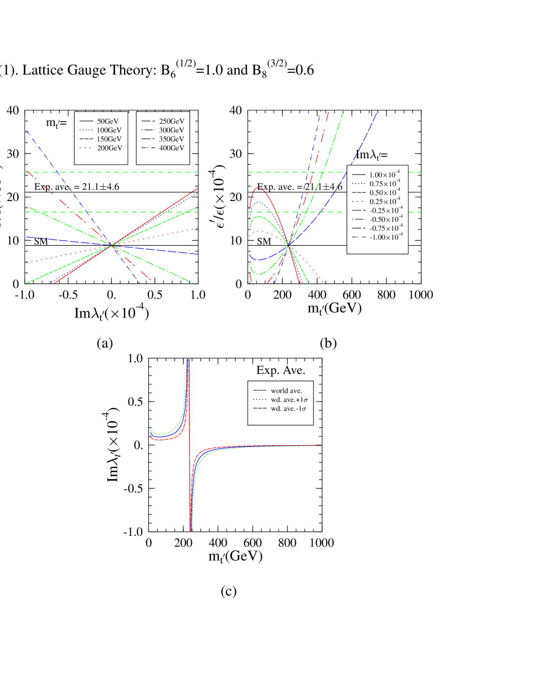
Figure 2: The Diagrams of (a) $\epsilon^{{}^{\prime}}/\epsilon$ to $\mbox{Im}\lambda_{t^{{}^{\prime}}}$, (b)$\epsilon^{{}^{\prime}}/\epsilon$ to $m_{t^{{}^{\prime}}}$ and (c) parameter space: $\mbox{Im}\lambda_{t^{{}^{\prime}}}$ to $m_{t^{{}^{\prime}}}$ with $B_{6}^{\rm(1/2)}$ and $B_{8}^{\rm(3/2)}$ in Lattice Gauge Theory.

References

- [1] A. Alavi-Harati et al., Phys. Rev. Lett. 83 (1999) 22.
- [2] V. Fanti et al., Phys. Lett. 465 (1999) 335.
- [3] U. Nierste, hep-ph/9910257; V. Fanti et al,
- [4] L. Wolfenstein, Phys. Rev. Lett. 13 (1964) 562.
- [5] M. Fabbrichesi; hep-ph/9909224, hep-ph/0002235; M. Jamin, hep-ph/9911390.
- [6] S. Bosch, A.J. Buras, M. GORBAHN, S. Jäger, M. Jamin, M.E. Lauteubacher and L. Silvestrni, hep-ph/9904408.
- [7] S. Bertolini, J.O. Eeg, M. Fabbrichesi, hep-ph/9802405.
- [8] Y.-Y. Keum, U. Nierste, and A.I. Sanda, hep-ph/9903230; T. Hambye, G.O. Khler, E.A. Paschos, and P.H. Soldan, hep-ph/9906434; S. Gardner and G. Valencia, hep-ph/9909202.
- [9] A.J. Buras, hep-ph/9806471.
- [10] G. Buchalla, A.J, Buras, M.E. Lautenbacher, Rev. of Mod. Phys. 68 (1996) 1125 and references therein; E. A. Paschos, Y.L. Wu, Mod. Phys. Lett. A6 (1991) 93.
- [11] C.Caso et al., (Particle Data Group), Eur. Phys. J. C3 (1998) 1.
- [12] G. Buchalla, A.J, Buras, M.E. Lautenbacher, Nucl. Phys. 408 (1993) 209.
- [13] R. Gupta, hep-ph/9801412; G. Kilcup, R.Gupta and S.R. Sharpe, Phys. Rev. D57 (1998) 1654; L. Conti, et al. hep-ph/9711053; T. Blum et al., hep-lat/9908025.
- [14] R. Gupta, T. Bhattacharaya and S.R. Sharpe, Phys. Rev. D55 (1997) 4036.
- [15] W.A. Bardeen, A.J. Buras and J.-M. Gerard, Phys. Lett. B180 (1986) 133; Nucl. Phys. B293 (1987) 787; Phys. Lett. B192 (1987) 138; J. Heinrich, E.A. Paschos, J.-M. Schwarz, and Y.L. Wu, Phys. Lett. B279 (1992) 140; Y.L. Wu, Int.J. Mod. Phys. A7 (1992) 2863; T. Hambye, G.O. Köhler, E.A. Paschos, P.H. Soldan and W.A. Bardeen, Phys. Rev. D58 (1998) 014017; W.A. Bardeen, Nucl. Phys. Proc. Suppl. 7A (1989) 149.
- [16] D. Espriu, E. de Rafael and J. Taron, Nucl. Phys. B345 (1990) 22; J. Bijnens, Phys. Rept. 265 (1996) 369; S. Bertolini, J.O. Eeg, M. Fabbrichesi, Nucl. Phys. B449 (1995) 197; Nucl. Phys. B476 (1996) 225; hep-ph/9802405; S. Bertolini, J.O. Eeg, M. Fabbrichesi and E.I. Lashin, Nucl. Phys. B514 (1998) 93.
- [17] M. Faggrichesi, hep-ph/9909224.
- [18] Y. Grossman, Y. Nir and R. Rattazzi, Hep-ph/9701231.
- [19] A.J. Buras, et al.,hep-ph/9908371; A.L. Kagan and M.Neubert, hep-ph/9908404; A.Masiero and H. Murayama, hep-ph/9903363; Chao-Shang Huang and Wei Liao, hep-ph/9908246, hep-ph/0001174 ; M. Brhlik et al., hep-ph/9909480; S. Baek and P. Ko, hep-ph/9909433; D.A. Demir, A. Masiero, O. Vives, hep-ph/9909325.
- [20] Y. Nir and H.R. Quinn, Ann. Rev. Nucl. Part. Sci. 42 (1992) 211; Phys. Rev. D42 (1990) 1473; Y. Nir and D. Silverman, Nucl. Phys. B345 (1990) 301; I. Dunietz, Ann. Phys. 184 (1988) 350; C.O. Dib, D.london and Y. Nir, Int. J. Mod. Phys. A6 (1991)1253; J.P. Silva and L. Wolfenstein, hep-ph/9610208; Y. Grossman and M.P. Worah, Phys. Lett. B395 (1997) 241.
- [21] Y.L. Wu and L. Wolfenstein, Phys. Rev. lett. 73, 1762 (1994); L. Wolfenstein and Y.L. Wu , Phys. Rev. lett. 73, 2809 (1994); S. Weinberg, Phys. Rev. D42 (1990) 860; L. Lavoura, Int. J. Mod. Phys. A8 (1993)375; Chao-Shang Huang and Shou-Hua Zhou, Phys. Rev. D61 (2000) 015011
- [22] D. Chang, Nucl.Phys. B214 (1983) 435; H.Harari and M. Leurer, Nucl. Phys. B233 (1984) 221; M. Leurer, Nucl. phys. B226 (1986) 147; X.G. He, hep-ph/9903242.
- [23] Y. Nir and D. Silverman, Phys. Rev. D42 (1990) 1477; W-S, Choong and D. Silverman, Phys. Rev. D49 (1994) 2322; L.T. Handoko, Hep-ph/9708447.
- [24] V. Barger, Y.B. Dai, K. Whisnant and B.L. Young, Hep-ph/9901380; R.N. Mohapatra, hep-ph/9702229; S. Mohanty, D.P. Roy and U. Sarkar, hep-ph/9810309; S.C. Gibbons,et al., Phys. lett. B430 (1998) 296; V. Barger, K. Whisnant and T.J. Weiler, Phys. lett. B427, (1998) 97; V. Barger, S. Pakvasa, T.J. Weiler and K. Whisnant, Phys. Rev. D58 (1998) 093016.
- [25] K.C. Chou, Y.L. Wu, and Y.B. Xie, Chinese Phys. Lett. 1 (1984) 2.
- [26] J.F. Gunion, Douglas W. McKay, H. Pois, Phys. Lett. B334 (1994) 339; Phys. Rev. D51 (1995) 201.
- [27] references therein of Ref.[35].
- [28] R.S. Willey, Phys. Rev. D44 (1991) 3646; H. Veltman and M. Veltman, Acta Phys. Pol. B22 (1991) 669.
- [29] T.N. Truong, Phys. Rev. Lett. 70 (1993) 888.
- [30] S.R. Beane and S. Varma, hep-ph/9304233.
- [31] W.J. Marciano, Phys. Rev. D60 (1999) 093006
- [32] J. Erler and P. Langacker, http://www-pdg.lbl.gov/1999/stanmodelrpp.ps.
- [33] Mark II Collab., G.S. Abrams et al., Phys. Rev. Lett. 63(1989) 2173; L3 Collab., B. Advera et al., Phys. Lett. B231 (1989) 509; OPAL Collab., I. Decamp et al., ibid., 231 (1989) 519; DELPHI Collab., M.Z. Akrawy et al., ibid., 231 (1989) 539.
- [34] Z. Berezhiani and E, Nardi, Phys. Rev. D52 (1995) 3087; C.T. Hill, E.A. Paschos, Phys. Lett. B241 (1990) 96.
- [35] C.S. Huang, W. J. Huo and Y.L. Wu, Mod. Phys. Lett. A14 (1999)2453.
- [36] R. D. Peccei, hep-ph/9909236; T. Hattori, T. Hasuike and S. Wakaizumi, hep-ph/9808412; A.J. Buras, hep-ph/9901409.
- [37] S. Adler, et al., Phys. Rev. Lett. B76 (1996) 1421.
- [38] J. Adams,it et al,. hep-ex/9806007.
- [39] A.P. Heinson, et al., Phys. Rev. D51 (1995) 985.
- [40] Y. Grossman and Y. Nir. Phys. Lett. B398 (1997) 163.
- [41] T. Akagi, et al., Phys. Rev. D51 (1995) 2061.
- [42] F. Gabbiani, hep-ph/9901262.
- [43] G. Buchalla, A.J. Buras, hep-ph/9901288.
- [44] S. Adler, et al., Phys. Rev. Lett. B79 (1997) 2204.
- [45] L. Littenberg, Phys. Rev. D39 (1989) 3322.
- [46] G. Buchalla, A.J. Buras, Nucl. Phys. B400 (1993) 225; B548 (1999) 309.
- [47] T. Hattori, T. Hasuike, S. Wakaizumi, hep-ph/9804412.
- [48] G.W. Kilcup, Nucl. Phys. (Proc. Suppl.) B20 (1991 417; S.R. Sharpe, ibid., 429; D. Pekurovsky and G.Kilcup, hep-lat/9709146.