Real-time nonequilibrium dynamics in hot QED plasmas:
dynamical renormalization group approach

Abstract

We study the real-time nonequilibrium dynamics in hot QED plasmas implementing a dynamical renormalization group and using the hard thermal loop (HTL) approximation. The focus is on the study of the relaxation of gauge and fermionic mean fields and on the quantum kinetics of the photon and fermion distribution functions. For semihard photons of momentum $eT\ll k\ll T$ we find to leading order in the HTL that the gauge mean field relaxes in time with a power law as a result of infrared enhancement of the spectral density near the Landau damping threshold. The distribution function of semihard photons in linear response also relaxes with a power law, with a power that is twice that for the mean field. The dynamical renormalization group reveals the emergence of detailed balance for microscopic time scales larger than $1/k$ while the rates are still varying with time. The quantum kinetic equation for the photon distribution function allows us to study photon production from a thermalized quark-gluon plasma (QGP) by off-shell effects. We find that for a QGP of temperature $T\sim 200\;\mbox{MeV}$ and lifetime $10\lesssim t\lesssim 50\;\mbox{fm}/c$ the hard ($k\sim T$) photon production from off-shell bremsstrahlung ($q\rightarrow q\gamma$ and $\bar{q}\rightarrow\bar{q}\gamma$) at ${\cal O}(\alpha)$ grows logarithmically in time and is comparable to that produced from on-shell Compton scattering and pair annihilation at ${\cal O}(\alpha\,\alpha_{s})$. Hard fermion mean fields relax as $e^{-\alpha\,T\,t\,\ln(\omega_{P}t)}$ with $\omega_{P}=eT/3$ the plasma frequency, as a consequence of the emission and absorption of soft magnetic photons. A quantum kinetic equation for hard fermions is obtained directly in real time from a field theoretical approach improved by the dynamical renormalization group. The collision kernel is time-dependent and infrared finite. In linear response the fermion distribution function relaxes with an anomalous exponential law with an exponent twice as large as that for the mean field.

I Introduction

The study of nonequilibrium phenomena under extreme conditions play a fundamental role in the understanding of ultrarelativistic heavy ion collisions and early universe cosmology. Forthcoming relativistic heavy ion experiments at BNL Relativistic Heavy Ion Collider (RHIC) and CERN Large Hadron Collider (LHC) aim to search for a deconfined phase of quarks and gluons, the quark gluon plasma (QGP), which is predicted by lattice QCD simulations [1, 2] to emerge at a temperature scale $T\gtrsim 200\;\mbox{MeV}$.

Recent results from CERN Super Proton Synchrotron (SPS) [3] seem to confirm the main theoretical ideas that in the central region in ultrarelativistic heavy ion collision a deconfined plasma of quarks and gluons forms which expands and cools rapidly and eventually hadronizes.

Current estimates based on energy deposited in the central region for $\sqrt{s}/\text{nucleon-pair}\sim 200\;{\rm GeV}$ at RHIC suggest that the lifetime of a deconfined QGP is of order $10-50~{}\mbox{fm}/c$ [1, 2]. At such unprecedented short time scales, an important aspect is an assessment of thermalization time scales and the potential for non-equilibrium effects associated with the rapid expansion and finite lifetime of the plasma and their impact on experimental observables. Lattice QCD is simply unable to deal with these questions because simulations are restricted to thermodynamic equilibrium quantities and a field-theoretical nonequilibrium approach is needed for an accurate description of the formation and evolution of the QGP. An important and pioneering step in this direction was undertaken by Geiger [4] who applied transport methods combined with perturbative QCD (pQCD) to obtain a quantitative picture of the evolution of partons in the early stages of formation and evolution of the plasma.

The consistent study of the evolution of partons in terms of pQCD cross sections that include screening corrections to avoid the infrared divergences associated with small angle scattering lead to the conclusion that quarks and gluons thermalize on time scales of a few $\mbox{fm}/c$ [5]. The necessity of a deeper understanding of equilibrium and non-equilibrium aspects of the quark-gluon plasma motivated an intense study of the abelian and non-abelian plasmas in extreme environments. A major step towards a consistent description of non-perturbative aspects was taken by Braaten and Pisarski [6, 7, 8, 9, 10], who introduced a novel resummation method that re-organizes the perturbative expansion in terms of the degrees of freedom associated with collective modes [9], rather than bare particles. This program, called the hard thermal loop or HTL program is now at the heart of most treatments of equilibrium aspects of abelian and non-abelian plasmas [11].

Thermal field theory provides the tools to study the properties of plasmas in equilibrium [11, 12, 13, 14], but the consistent study of nonequilibrium phenomena in real time requires the methods of nonequilibrium field theory [15] (see also Refs. [16, 17] for further references). The study of the equilibrium and nonequilibrium properties of abelian and non-abelian plasmas as applied to the QGP has as ultimate goal a deeper understanding of the potential experimental signatures of the formation and evolution of the QGP in ultrarelativistic heavy ion collisions. Amongst these, photons and dileptons (electron and/or muon pairs) produced during the early stages of the QGP are considered as some of the most promising signals [18, 19, 20]. Since photons and lepton pairs interact electromagnetically their mean free paths are longer than the estimated size of the QGP fireball $\sim 10-50\;\mbox{fm}$ and unlike hadronic signals they do not undergo final state interactions. Therefore photons and dileptons produced during the early stages of QGP carry clean information from this phase.

The goals of this work. In this work we aim to provide a comprehensive study of several relevant aspects of the nonequilibrium dynamics of an abelian QED plasma in real time. Many features of full QCD are similar to those of the abelian (QED) theory[6, 11, 9], in particular leading contributions in the HTL limit can be straighfordarly generalized from QED to QCD, thus the leading results for relaxation and photon production from a QGP[19, 20] can be understood from the study of a QED plasma.

We utilize a gauge invariant formulation, available in abelian gauge theories that circumvents the possible ambiguities associated with gauge invariance [30, 31]. Thus gauge and fermionic mean fields and distribution functions are automatically gauge invariant. We implement and apply the method of the dynamical renormalization group, introduced recently to study non-equilibrium phenomena directly in real time [21, 22] to extract a consistent, non-perturbative description of real-time dynamics out of equilibrium.

In particular we focus on the following:

• The real time evolution of gauge mean fields in linear response in the HTL approximation. The goal here is to study directly in real time the relaxation of (coherent) gauge field configurations in the linearized approximation to leading order in the HTL program. Whereas a similar study has been carried out in scalar QED [23] and confirmed numerically in [24] the most relevant case of spinor QED has not yet been studied in detail.

• The quantum kinetic equation that describes the evolution of the distribution function of photons in the medium, again to leading order in the HTL approximation. This aspect is relevant to study photon production via off-shell effects directly in real time. As explained in detail, this quantum kinetic equation, obtained from a microscopic field theoretical approach based on the dynamical renormalization group [21, 22] displays novel off-shell effects that cannot be captured via the usual kinetic description that assumes completed collisions [18, 19, 20].

• The evolution in real time of fermionic mean fields features anomalous relaxation arising from the emission and absorption of magnetic photons (gluons) which are only dynamically screened by Landau damping [10, 25, 26]. The fermion propagator was studied previously in real time in the Bloch-Nordsieck approximation which provides a resummation of the infrared divergences associated with soft photon (or gluon) bremsstrahlung in the medium [25, 26]. In this article we implement the dynamical renormalization group to study the evolution of fermionic mean fields providing an alternative to the Bloch-Nordsieck treatment.

• We obtain the quantum kinetic equation for the fermionic distribution function for hard fermions via the implementation of the dynamical renormalization group. There has recently been an important effort in trying to obtain the effective kinetic (Boltzmann) equations for hard charged (quasi)particles [27, 28, 29] but the collision kernel in this equation features the logarithmic divergences associated with the emission and absorption of soft magnetic photons (or gluons) [29]. The dynamical renormalization group leads to a quantum kinetic equation directly in real time bypassing the assumption of completed collisions and leads to a time-dependent collision kernel free of infrared divergences.

Summary of the main results. The main results of this study are summarized as follows.

• Relaxation of gauge mean fields. We studied the relaxation of a gauge mean field in linear response to leading order in the HTL approximation both for soft momentum $k\lesssim eT$ and for semihard momentum $eT\ll k\ll T$ under the assumption of weak electromagnetic coupling.

  Soft momentum ($k\sim eT$): in this case the relaxation of the gauge mean field is dominated by the end-point contribution of the Landau damping cut. As a consequence, the soft gauge mean field relaxes with a power law long time tail of the form

  $${\bf a}_{T}({\bf k},t)\buildrel kt\gg 1\over{=}{\bf a}_{T}({\bf k},0)\left[\frac{k^{2}Z_{T}(k)}{\omega^{2}_{T}(k)}\cos[\omega_{T}(k)t]-\frac{12}{e^{2}T^{2}}\frac{\cos kt}{t^{2}}\right]\;,$$

  where $\omega_{T}(k)$ is the transverse photon pole and $Z_{T}(k)$ is the corresponding residue. We note that in spite of the power law tail the gauge mean field relaxes towards the oscillatory mode determined by the transverse photon pole. This reveals that the soft collective excitation in a plasma is stable in the HTL approximation.

  Ultrasoft momentum ($k\ll eT$): In the region of ultrasoft momentum the spectral density divided by the frequency features a sharp Breit-Wigner peak near zero frequency in the region of Landau damping, with width $\Gamma_{k}=12k^{3}/\pi e^{2}T^{2}$. We find that the amplitude of a mean field of transverse photons prepared via a source that is adiabatically switched-on is given by

  $${\bf a}_{T}({\bf k},t)\buildrel kt\gg 1\,,\,\Gamma_{k}\,t\lesssim 1\over{=}{\bf a}_{T}({\bf k},0)\left[\frac{k^{2}Z_{T}(k)}{\omega^{2}_{T}(k)}\cos[\omega_{T}(k)t]+e^{-\Gamma_{k}t}\right]\;.$$

  We emphasize that the exponential decay is a consequence of the sharp resonance near zero frequency in the Landau damping region of the spectral density and only arises if the mean field is prepared by an external source whose time Fourier transform has a simple pole at zero frequency, such is the case for an adiabatically prepared initial state. This result confirms those found numerically in Ref. [24].

  Semi-hard momentum ($eT\ll k\ll T$): In this region both the HTL approximation and the perturbative expansion are formally valid. However the spectral density in the Landau damping region is sharply peaked near $\omega=k$ and the transverse photon pole approaches the edge of the Landau damping region from above. We find that although the perturbative expansion is in principle valid, the sharp spectral density near the edge of the continuum results in a breakdown of the perturbative expansion. The dynamical renormalization group provides a consistent resummation of the lowest order HTL perturbative contributions in real time, leading to the following relaxation of the mean field at intermediate asymptotic times:

  $${\bf a}_{T}({\bf k},t)\buildrel kt\gg 1\over{=}\mathchoice{{\hbox{\boldmath$\displaystyle\cal A$}}}{{\hbox{\boldmath$\textstyle\cal A$}}}{{\hbox{\boldmath$\scriptstyle\cal A$}}}{{\hbox{\boldmath$\scriptscriptstyle\cal A$}}}_{T}({\bf k},t)\left(\frac{t}{\tau_{0}}\right)^{-\frac{e^{2}T^{2}}{12k^{2}}}\;,$$

  where $\tau_{0}\sim 1/k$ and $\mathchoice{{\hbox{\boldmath$\displaystyle\cal A$}}}{{\hbox{\boldmath$\textstyle\cal A$}}}{{\hbox{\boldmath$\scriptstyle\cal A$}}}{{\hbox{\boldmath$\scriptscriptstyle\cal A$}}}_{T}({\bf k},t)$ is an oscillating function. The anomalous exponent is a consequence of an infrared enhancement arising from the sharp spectral density near the threshold of the Landau damping region for semihard momentum. The crossover to exponential relaxation due to collisional processes at higher orders is discussed.

• Quantum kinetic equation for the photon distribution function. Using the techniques of nonequilibrium field theory and the dynamical renormalization group, we obtain the quantum kinetic equation for the distribution function of semihard photons $eT\ll k\ll T$ to lowest order in the HTL approximation assuming that the fermions are thermalized. An important result is that the collision kernel is time-dependent and the dynamical renormalization group reveals that detailed balance emerges during microscopic time scales, i.e, much shorter than the relaxation scales. In the linearized approximation we find that the departure from equilibrium of the photon distribution function relaxes as:

  $$\delta n^{\gamma}_{\bf k}(t)=\delta n^{\gamma}_{\bf k}(t_{0})\left(\frac{t-t_{0}}{\tau_{0}}\right)^{-\frac{e^{2}T^{2}}{6k^{2}}}\quad\mbox{for}\quad k(t-t_{0})\gg 1\;,$$

  where $\tau_{0}\sim 1/k$, and $t_{0}$ is the initial time. Furthermore, this quantum kinetic equation allows us to study photon production by off-shell effects, which to leading order in the HTL approximation are determined by photon bremsstrahlung and is of order $\alpha$. Extrapolating the result from QED to thermalized QGP with two flavors of light quarks, we find that the total number of hard photons at time $t$ per invariant phase space volume to lowest order is

  $$N(t)=\frac{5\alpha T^{3}}{18\pi^{2}k^{2}}\left\{\ln\left[2k(t-t_{0})\right]+\gamma_{E}-1\right\}\quad\mbox{for}\quad k(t-t_{0})>1\;.$$

  with $t_{0}\approx 1\mbox{fm/c}$ is the time scale at which the QGP plasma is thermalized.

  We find that for a quark-gluon plasma at temperature $T\sim 200\;\mbox{MeV}$ and of lifetime $10\lesssim(t-t_{0})\lesssim 50\;\mbox{fm}/c$, the hard ($k\sim T$) photon production by off-shell bremsstrahlung is comparable to that from Compton scattering and pair annihilation of order $\alpha\,\alpha_{s}$ [19, 20].

• Relaxation of fermion mean fields. We implement the dynamical renormalization group resummation to study the real-time relaxation of a fermion mean field for hard momentum. The emission and absorption of magnetic photons which are only dynamically screened by Landau damping introduce a logarithmic divergence in the spectral density near the fermion mass shell. The dynamical renormalization group resums these divergences in real time and leads to a relaxation of the fermion mean field for hard momentum given by:

  $$\psi({\bf k},t)\buildrel kt\gg 1\over{=}e^{-\alpha Tt\left[\ln(\omega_{P}t)+0.12652\ldots\right]}\times\mbox{oscillating phases},$$

  with $\omega_{P}$ being the plasma frequency.

• Quantum kinetics for the fermion distribution function. We obtain a quantum kinetic equation for the distribution function of hard fermions using non-equilibrium field theory and the dynamical renormalization group resummation. Assuming thermalized photons we find that the collision kernel is infrared finite but time-dependent. In the linearized approximation the distribution function relaxes as:

  $$\delta n^{f}_{\bf k}(t)\buildrel kt\gg 1\over{=}\delta n^{f}_{\bf k}(t_{0})\;e^{-2\alpha T(t-t_{0})\,\left[\ln(\omega_{P}t)+0.12652\ldots\right]}\;,$$

  where the anomalous relaxation exponent is twice that of the mean field.

The article is organized as follows. In Sec. II we review the main ingredients of nonequilibrium field theory, the initial value problem formulation for relaxation of nonequilibrium mean fields, and the dynamical renormalization group approach to quantum kinetics. In Sec. III we first study relaxation of the photon mean field in the hard thermal loop limit for soft $k\leq eT$ and semihard $eT\ll k\ll T$ photon momentum and obtain the quantum kinetic equation for the (hard and semihard) photon distribution function. In Sec. IV we study relaxation of fermionic mean fields for hard momentum and the quantum kinetic equation for the fermion distribution function. Our conclusions and some further questions are presented in Sec. V.

II General Aspects

As stated in the introduction our goal is to provide a systematic study of non-equilibrium phenomena in a hot abelian plasma. In particular we focus on a detailed study of the real time relaxation of expectation values of fermions and gauge bosons, i.e, fermionic and gauge mean fields as well as the quantum kinetics for the evolution of the expectation value of the number operator associated with fermions and photons. A fundamental issue that must be addressed prior to setting up our study is that of gauge invariance. In the abelian case it is straightforward to reduce the Hilbert space to the gauge invariant subspace and to define gauge invariant charged fermionic operators. The description in terms of gauge invariant states and operators is best achieved within the canonical formulation which begins with the identification of the canonical field and conjugate momenta and the primary and secondary first class constraints associated with gauge invariance. The physical states are those annihilated by the constraints and physical operators commute with the (first class) constraints. This program has been implemented explicitly in the case of scalar quantum electrodynamics [22, 30] and the fermionic case can be treated in the same manner with few minor technical modifications.

The final result of this formulation is that the Hamiltonian acting on the gauge invariant states and written in terms of gauge invariant fields is exactly equivalent to that obtained in Coulomb gauge, which is the statement that Coulomb gauge describes the theory in terms of the physical degrees of freedom. Furthermore the instantaneous Coulomb interaction can be traded for a Lagrange multiplier [22] leading to the following Lagrangian density

$${\cal L} = \bar{\Psi}\left(i{\not\!{\partial}}-e\gamma_{0}A_{0}+e{\mathchoice{{\hbox{\boldmath$\displaystyle\gamma$}}}{{\hbox{\boldmath$\textstyle\gamma$}}}{{\hbox{\boldmath$\scriptstyle\gamma$}}}{{\hbox{\boldmath$\scriptscriptstyle\gamma$}}}}\cdot{\bf A}_{T}-m\right)\Psi+\frac{1}{2}\left[\left(\partial_{\mu}{\bf A}_{T}\right)^{2}+\left(\nabla A_{0}\right)^{2}\right]\;.$$

where ${\bf A}_{T}$ is the transverse component of the vector potential and $A_{0}$ is not to be interpreted as the time component of the gauge vector potential but is the Lagrange multiplier associated with the instantaneous Coulomb interaction. We emphasize that the fermionic charged fields $\Psi$ as well as the Lagrange multiplier $A_{0}$ are gauge invariant fields (see Refs. [22, 30]).

The fully renormalized equations of motion for the mean fields can be obtained by following the formulation presented in Refs. [31, 32]. However, the counterterms that eliminate the zero temperature ultraviolet divergences are temperature independent [11] and play no rôle in the present context, thus we will neglect the zero temperature renormalization counterterms in our study.

Furthermore we consider a neutral plasma (i.e, with zero chemical potential for the charged fields) at a temperature $T\gg m$ with $m$ the (renormalized) mass of the fermions, hence in what follows we neglect the fermion mass unless otherwise stated.

A Nonequilibrium Field Theory

The formulation of nonequilibrium quantum field theory in terms of the Schwinger-Keldysh or the closed-time-path (CTP) is standard [15, 16, 17]. A path integral representation requires a contour in the complex time plane, running forward and then backwards in time corresponding to the unitary time evolution of an initially prepared density matrix, with an effective Lagrangian in terms of fields on the different branches of the path

$${\cal L}_{\rm noneq}={\cal L}[\Psi^{+},\bar{\Psi}^{+},A^{+}_{T},A^{+}_{0}]-{\cal L}[\Psi^{-},\bar{\Psi}^{-},A^{-}_{T},A^{-}_{0}]\;,$$

where the “$+$” (“$-$”) superscripts for the fields refer to fields defined in the forward (backward) time branches. This description leads to a straightforward diagrammatic expansion of the nonequilibrium Green’s functions in terms of real-time propagators but with modified Feynman rules (as compared to standard field theory) [15, 16, 17]. The free fermion and photon propagators are given in detail in the Appendix.

Since we study two different type of situations: (i) the relaxation of expectation values in the linearized approximation (linear response) and (ii) the kinetic equation that describes the evolution of a non-equilibrium distribution function, we make a distinction between the real-time propagators used in each case.

• In the case of relaxation of expectation values in linear response, the distribution functions that enter in the fermion and photon propagators (125)-(135) are those with equilibrium distributions.

• When we study the kinetic equations for the expectation value of the fermion number and photon number operators, we assume that the initial density matrix is diagonal in the basis of the quasiparticles (see below) but with nonequilibrium initial distributions. Thus the propagators obtained with this initial density matrix have the free-field form, as given in (125)-(135) but the initial occupation numbers are not the equilibrium Fermi-Dirac or Bose-Einstein distribution.

B Real-time relaxation of mean fields in linear response

The mean fields under consideration are the expectation value of either fermion or gauge field operators in the nonequilibrium state induced by the external source. Obviously in equilibrium and in the absence of external sources these must vanish, and we introduce time-dependent sources to induce an expectation value of these operators. Our strategy to study the relaxation of these mean fields as an initial value problem is to prepare these mean fields via the adiabatic switching-on of an external current[31, 32, 33]. Once the current is switched off the expectation values must relax towards equilibrium and we study this real-time evolution. This formulation to study the real-time evolution of mean fields has the advantage that it leads to a straightforward and systematic implementation of the dynamical renormalization group method as explained in detail in Refs. [21, 22].

The initial value problem formulation for studying the linear relaxation of the mean fields begins by introducing c-number external sources coupled to the quantum fields. Let $\eta(x)$ be the Grassmann-valued fermionic source and ${\bf J}_{T}(x)$ be the electromagnetic sources, then the Lagrangian density becomes

$${\cal L}\rightarrow{\cal L}+\bar{\Psi}\eta+\bar{\eta}\Psi+{\bf J}_{T}\cdot{\bf A}_{T}\;.$$

The presence of external sources will induce responses of the system. Let $\Phi(x)$ be a generic quantum field (i.e., fermionic or bosonic) with $\Phi^{\pm}(x)$ the fields defined on the forward and backward branches, respectively, and $J(x)$ the corresponding c-number external source (the same for both branches). The expectation value of $\Phi(x)$ induced by $J(x)$ in a linear response analysis is given by

$$\phi({\bf x},t) \equiv \langle\Phi^{\pm}({\bf x},t)\rangle_{J}$$ (1)

$$= \int d^{3}x^{\prime}\int_{-\infty}^{+\infty}dt^{\prime}\;G_{\rm ret}({\bf x},t;{\bf x^{\prime}},t^{\prime})\;J({\bf x^{\prime}},t^{\prime})\;,$$ (2)

with the retarded Green’s function

$$G_{\rm ret}({\bf x},t;{\bf x^{\prime}},t^{\prime}) \equiv i\Big{[}\left\langle\Phi^{+}({\bf x},t)\bar{\Phi}^{+}({\bf x^{\prime}},t^{\prime})\right\rangle-\left\langle\Phi^{+}({\bf x},t)\bar{\Phi}^{-}({\bf x^{\prime}},t^{\prime})\right\rangle\Big{]}$$ (3)

$$= i\left\langle\left[\Phi({\bf x},t),\bar{\Phi}({\bf x^{\prime}},t^{\prime})\right]_{\mp}\right\rangle\theta(t-t^{\prime})\;,$$ (4)

where expectation values are computed in the CTP formulation in the full interacting theory but with vanishing external source, $\theta(t-t^{\prime})$ is the step function and the subscripts $\mp$ refer to the commutator ($-$) for bosonic or anticommutator ($+$) for fermionic fields.

A practically useful initial value problem formulation for the real-time relaxation of mean fields is obtained by considering that the external source is adiabatically switched on in time at $t=-\infty$ and suddenly switched off at $t=t_{0}$, i.e.,

$$J({\bf x},t)=J({\bf x})\;e^{\epsilon(t-t_{0})}\;\theta(t_{0}-t)\;,\quad\epsilon\rightarrow 0^{+}\;.$$ (5)

The adiabatic switching on of the external source induces a mean field that is dressed adiabatically by the interaction. Then for $t>t_{0}$, after the external current has been switched off, the mean field will relax towards equilibrium, and our aim is to study this relaxation directly in real time [33].

The equations of motion of the mean fields are obtained via the tadpole method [17] and are automatically causal and retarded. The central idea of the tadpole method is to write the field into a c-numbered expectation value plus fluctuations around it, i.e., writing

$$\Phi^{\pm}({\bf x},t)=\phi({\bf x},t)+\chi^{\pm}({\bf x},t)\quad\mbox{with}\quad\langle\Phi^{\pm}({\bf x},t)\rangle_{J}=\phi({\bf x},t)\;.$$

The equation of motion for $\phi({\bf x},t)$ is obtained by requiring $\langle\chi^{\pm}({\bf x},t)\rangle=0$ to all orders in perturbation theory.

For the study of relaxation of the mean fields, we assume that at $t=-\infty$ the system is in thermal equilibrium at a temperature $T$ and henceforth choose $t_{0}=0$ for convenience. The retarded and the equilibrium (i.e., time translational invariant) nature of $G_{\rm ret}({\bf x},t;{\bf x^{\prime}},t^{\prime})$ and the adiabatic switching on of $J({\bf x},t)$ entail that

$$\begin{array}[]{l}\phi({\bf x},t=0)=\phi_{0}({\bf x}),\vspace{5pt}\\ \dot{\phi}({\bf x},t<0)=0\;,\end{array}$$ (6)

where $\phi_{0}({\bf x})$ is determined by $J({\bf x})$ (or vice versa). It is worth pointing out that $\dot{\phi}({\bf x},t)$ is not specified at $t=0$ although $\dot{\phi}({\bf x},t<0)=0$. This is because the external source is switched off at $t=0$.

C Main ingredients for quantum kinetics

In Ref. [22] a systematic treatment to obtain the kinetic equation that determines the real-time evolution of the distribution function (defined as the expectation value of the number operator) was established, leading to its interpretation as a dynamical renormalization group equation. Here we summarize the basic steps to obtain the relevant quantum kinetic equations from first principles and we refer the reader to Ref. [22] for more details.

• Identify the proper degrees of freedom (quasiparticles) to be described by the kinetic equation, the corresponding microscopic time scale $\tau_{\rm micro}$ associated with their oscillation, and the number operator $N({\bf k},t)$ that counts these degrees of freedom with momentum ${\bf k}$ at time $t$.

• Use the Heisenberg equations of motion to derive a general rate equation for $d{n}_{\bf k}(t)/dt$ with $n_{\bf k}(t)=\langle N({\bf k},t)\rangle$, where the expectation value is taken in the initial density matrix. Assuming that the initial density matrix is diagonal in the basis of free quasiparticles but with nonequilibrium distribution functions, we can expand the rate equation in perturbation theory using nonequilibrium Feynman rules and free real-time propagators in terms of nonequilibrium distribution functions. Since the resulting expression is a functional of the distribution function at initial time, the solution of the kinetic equation can be obtained by direct integration.

  This solution is typically characterized by the emergence of secular terms, i.e, terms that grow in time in the intermediate asymptotic regime ($\tau_{\rm micro}\ll t\ll\tau_{\rm rel}$) where the scale $\tau_{\rm rel}$ is that at which perturbation theory breaks down [21, 22].

• These secular terms growing in time become divergent if the perturbative solution is extrapolated to long times. However, perturbation theory is valid and dominated by the secular terms during the intermediate asymptotic time scales $\tau_{\rm micro}\ll t\ll\tau_{\rm rel}$. The dynamical renormalization group is used to resum the secular terms through a renormalization of the initial distribution functions. This introduces an arbitrary time scale $\tau$ which serves as a renormalization point. The $\tau$-independence of the renormalized solution leads to the dynamical renormalization equation [21, 22]. This dynamical renormalization equation describing the evolution of the quasiparticle distribution is recognized as the quantum kinetic equation.

III Photons out of equilibrium

In this section we study non-equilibrium aspects of photon relaxation and production. We begin by analyzing the relaxation in real time of a photon condensate in linear response both in the case of soft $k\lesssim eT$ and semihard (or semisoft) $eT\ll k\ll T$ assuming the electromagnetic coupling to be small. We then continue with a study of the production of semihard photons via off-shell effects.

A Relaxation of the gauge mean field

We begin with the relaxation of soft photons of momenta $k\sim eT$. As mentioned in the previous section, the equation of motion for the transverse photon mean field can be derived from the tadpole method [17] by decomposing the full quantum fields into c-number expectation values and quantum fluctuations around the expectation values:

$${\bf A}^{\pm}_{T}({\bf x},t) = {\bf a}_{T}({\bf x},t)+{\mathchoice{{\hbox{\boldmath$\displaystyle\cal A$}}}{{\hbox{\boldmath$\textstyle\cal A$}}}{{\hbox{\boldmath$\scriptstyle\cal A$}}}{{\hbox{\boldmath$\scriptscriptstyle\cal A$}}}}^{\pm}_{T}({\bf x},t),$$ (7)

$${\bf a}_{T}({\bf x},t) = \langle{\bf A}^{\pm}_{T}({\bf x},t)\rangle\;.$$ (8)

With the external source ${\bf J}_{T}({\bf x},t)$ of the adiabatic form (5) chosen to vanish at $t\geq 0$, we find the linear equation of motion for the spatial Fourier transform of ${\bf a}_{T}({\bf x},t)$ for $t\geq 0$ to be given by

$$\left(\frac{\partial^{2}}{\partial t^{2}}+k^{2}\right)\;{\bf a}_{T}({\bf k},t)+\int^{t}_{-\infty}dt^{\prime}\;\Pi_{T}({\bf k},t-t^{\prime})\;{\bf a}_{T}({\bf k},t^{\prime})=0\;,$$ (9)

where

$${\bf a}_{T}({\bf k},t)\equiv\int d^{3}x\;e^{-i{\bf k}\cdot{\bf x}}\;{\bf a}_{T}({\bf x},t)\;.$$

Here $\Pi_{T}({\bf k},t-t^{\prime})$ is the transverse part of the retarded photon self-energy and we have made explicit use of its retarded nature in writing Eq. (9), which evidently is causal and retarded.

Using the nonequilibrium Feynman rules and the real-time free fermion propagators given in the Appendix, we find the transverse polarization to be given by

$$\Pi_{T}({\bf k},t-t^{\prime}) = \int_{-\infty}^{+\infty}d\omega\;\rho_{T}(\omega,{\bf k})\sin[\omega(t-t^{\prime})]\;,$$ (10)

in terms of the spectral density to one-loop order

$$\rho_{T}(\omega,{\bf k}) = -e^{2}\int\frac{d^{3}q}{(2\pi)^{3}}\big{\{}[\delta(\omega-p-q)-\delta(\omega+p+q)][1+({\bf\hat{k}}\cdot{\bf\hat{p}})({\bf\hat{k}}\cdot{\bf\hat{q}})][1-n_{F}(p)-n_{F}(q)]$$ (12)

$$+\;[\delta(\omega-p+q)-\delta(\omega+p-q)][n_{F}(q)-n_{F}(p)][1-({\bf\hat{k}}\cdot{\bf\hat{p}})({\bf\hat{k}}\cdot{\bf\hat{q}})]\big{\}}\;,$$

where ${\bf p}={\bf k}+{\bf q}$.

It is now convenient to introduce an auxiliary quantity $\pi_{T}({\bf k},t-t^{\prime})$ as follows

$$\Pi_{T}({\bf k},t-t^{\prime})=\frac{\partial}{\partial t^{\prime}}\pi_{T}({\bf k},t-t^{\prime})\;.$$

and hence,

$$\pi_{T}({\bf k},t-t^{\prime})=\int_{-\infty}^{+\infty}{d\omega\over\omega}\rho_{T}(\omega,{\bf k})\cos[\omega(t-t^{\prime})]\;.$$

Upon integration by parts the equation of motion takes a form that displays clearly the nature of the initial value problem:

$$\left(\frac{\partial^{2}}{\partial t^{2}}+k^{2}\right){\bf a}_{T}({\bf k},t) - \int^{t}_{0}dt^{\prime}\;\pi_{T}({\bf k},t-t^{\prime})\;\dot{\bf a}_{T}({\bf k},t^{\prime})+\pi_{T}({\bf k},0)\;{\bf a}_{T}({\bf k},t)=0\;,$$ (13)

where a dot denotes derivative with respect to time and we used that $\dot{\bf a}_{T}({\bf k},t)=0$ for $t<0$. Eq. (13) together with the initial conditions specified at $t=0$ yields a well-defined initial value problem. As discussed above, the initial value ${\bf a}_{T}({\bf k},t=0)={\bf a}_{T}({\bf k},0)$ is determined by ${\bf J}_{T}({\bf k},t)$, and we choose

$$\dot{\bf a}_{T}({\bf k},t=0)=0$$ (14)

consistently with the adiabatic switching-on condition (6).

Eq. (13) can be solved by the Laplace transform method. We define,

$$\tilde{\bf a}_{T}(s,{\bf k}) = \int_{0}^{\infty}dt\;e^{-st}\;{\bf a}_{T}({\bf k},t)\;,$$ (15)

$$\tilde{\pi}_{T}(s,{\bf k}) = \int_{0}^{\infty}dt\;e^{-st}\;\pi_{T}({\bf k},t)\;,$$ (16)

with Re $\!s>0$. In terms of which the Laplace transform of the equation of motion leads to

$$\left[s^{2}+k^{2}+\tilde{\Pi}_{T}(s,{\bf k})\right]\tilde{\bf a}_{T}(s,{\bf k})=\left[s-\tilde{\pi}_{T}({s,\bf k})\right]{\bf a}_{T}({\bf k},0)\;,$$ (17)

where $\tilde{\Pi}_{T}(s,{\bf k})$ is the Laplace transform of ${\Pi}_{T}({\bf k},t-t^{\prime})$:

$$\tilde{\Pi}_{T}(s,{\bf k})=\pi_{T}({\bf k},0)-s\;\tilde{\pi}_{T}(s,{\bf k})\;.$$

The solution of Eq. (17) is given by

$$\tilde{\bf a}_{T}(s,{\bf k})=\frac{1}{s}\left\{1-\tilde{\Delta}_{T}(s,{\bf k})[k^{2}+\pi_{T}({\bf k},0)]\right\}{\bf a}_{T}({\bf k},0)\;,$$ (18)

where the retarded transverse photon propagator $\tilde{\Delta}_{T}(s,{\bf k})$ is given by

$$\tilde{\Delta}_{T}(s,{\bf k})=[s^{2}+k^{2}+\tilde{\Pi}_{T}(s,{\bf k})]^{-1}\;.$$ (19)

The real-time evolution of ${\bf a}_{T}({\bf k},t)$ is obtained by performing the inverse Laplace transform along the Bromwich contour which is to the right of all singularities of $\tilde{\bf a}_{T}(s,{\bf k})$ in the complex $s$-plane.

We note that this result is rather different from that obtained in Ref. [23] in the structure of the solution, in particular the prefactor $1/s$ in Eq. (18). This can be traced back to the different manner in which we have set up the initial value problem, as compared to the case studied in [23]. The adiabatic source (5) (for $t_{0}=0$) has a Fourier transform that has a simple pole in the frequency plane, this translates into the $1/s$ factor in Eq. (18). This particular case was not contemplated in those studied in Ref. [23] since the source (5) is not a regular function of the frequency. This difference will be seen to be at the heart of important aspects of relaxation of the mean field condensate in the soft momentum limit as discussed in detail below.

It is straightforward to see that the residue vanishes at $s=0$ in the solution (18). The singularities of $\tilde{\bf a}_{T}(s,{\bf k})$ are those arising from the retarded transverse photon propagator $\tilde{\Delta}_{T}(s,{\bf k})$.

1 Soft photons $k\sim eT$: real-time Landau damping

For soft photons of momenta $k\sim eT$, the leading ($\sim e^{2}T^{2}$) contribution to the photon self-energy arises from loop momenta of order $T$ and is referred to as a hard thermal loop (HTL) [6, 7]. In this region of momenta, the contribution of the fermion loop is non-perturbative.

In the HTL approximation ($s\sim k\ll q$), after some algebra we find that the HTL contribution to $\tilde{\Pi}_{T}(s,{\bf k})$ arises exclusively from the terms associated with $\delta(\omega\mp p\pm q)$ in Eq. (12) and reads

$$\tilde{\Pi}_{T}(s,{\bf k})=\frac{e^{2}T^{2}}{12}\left[\frac{is}{k}\left(1+\frac{s^{2}}{k^{2}}\right)\ln\frac{is+k}{is-k}-2\;\frac{s^{2}}{k^{2}}\right]\;.$$ (20)

The delta functions $\delta(\omega\mp p\pm q)$ have support below the light cone (i.e., $\omega^{2}<k^{2}$) and correspond to Landau damping processes [8] in which the soft photon scatters a hard fermion in the plasma.

The analytic continuation of $\tilde{\Pi}_{T}(s,{\bf k})$ in the complex $s$-plane is defined by

$$\Pi_{T}(\omega,{\bf k}) \equiv \tilde{\Pi}_{T}(s=-i\omega\pm 0^{+},{\bf k})=\mbox{Re}\Pi_{T}(\omega,{\bf k})\pm i\;\mbox{Im}\Pi_{T}(\omega,{\bf k}).$$ (21)

From Eq. (10) it is straightforward to see that the real and imaginary parts are related by the usual dispersion relation. The analytical continuation of $\tilde{\Delta}_{T}(s,{\bf k})$ and $\tilde{\pi}_{T}(s,{\bf k})$ can be defined analogously, and they are related to $\Pi_{T}(\omega,{\bf k})$ by

$$\Delta_{T}(\omega,{\bf k}) = -[\omega^{2}-k^{2}-\Pi_{T}(\omega,{\bf k})]^{-1}\;,$$

$$\mbox{Re}\Pi_{T}(\omega,{\bf k}) = \pi_{T}({\bf k},0)-\omega\;\mbox{Im}\pi_{T}(\omega,{\bf k})\;,$$

$$\mbox{Im}\Pi_{T}(\omega,{\bf k}) = \omega\;\mbox{Re}\pi_{T}(\omega,{\bf k})\;.$$

The analytical continuation of $\tilde{\Pi}_{T}(s,{\bf k})$ in the HTL limit thus reads

$$\Pi_{T}(\omega,{\bf k}) = \frac{e^{2}T^{2}}{12}\left[2\frac{\omega^{2}}{k^{2}}+\frac{\omega}{k}\left(1-\frac{\omega^{2}}{k^{2}}\right)\ln\left|\frac{\omega+k}{\omega-k}\right|\right]$$ (23)

$$-\;i\frac{\pi e^{2}T^{2}}{12}\frac{\omega}{k}\left(1-\frac{\omega^{2}}{k^{2}}\right)\theta(k^{2}-\omega^{2})\;.$$

In the HTL limit it is straightforward to prove that $\pi_{T}({\bf k},0)=0$. We note that $\mbox{Im}\Pi_{T}(\omega,{\bf k})$ only has support below the light cone and vanishes linearly as $\omega\rightarrow k$ from below. Since for soft momenta $k\ll eT$ the HTL photon self-energy is comparable in magnitude to or larger than the free inverse propagator, it has to be treated nonperturbatively.

Isolated poles of $\Delta_{T}(\omega,{\bf k})$ in the complex $\omega$-plane correspond to collective excitations. The transverse photon pole $\omega_{T}(k)$ is real and determined by [11]

$$\omega^{2}_{T}(k)-k^{2}-\mbox{Re}\Pi_{T}[\omega_{T}(k),{\bf k}]=0\;.$$

For ultrasoft photons $k\ll eT$, the dispersion relation of the collective excitations is [11]

$$\omega_{T}^{2}(k)=\omega_{P}^{2}+\frac{6}{5}k^{2}+{\cal O}\left({k^{4}\over e^{2}\,T^{2}}\right)\;,$$

where $\omega_{P}=eT/3$ is the plasma frequency. Consequently, the retarded transverse photon propagator $\tilde{\Delta}_{T}(s,{\bf k})$ has two isolated poles at $s=\pm i\omega_{T}(k)$ and a branch cut from $s=-ik$ to $s=ik$.

Having analyzed the analytic structure of $\tilde{\Delta}_{T}(s,{\bf k})$, we can now perform the integral along the Bromwich contour to obtain the real-time evolution of ${\bf a}_{T}({\bf k},t)$. Closing the contour in the half-plane $\mbox{Re}\;\!s<0$, we find ${\bf a}_{T}({\bf k},t)$ for $t>0$ to be given by

$${\bf a}_{T}({\bf k},t)={\bf a}^{\it pole}_{T}({\bf k},t)+{\bf a}^{\it cut}_{T}({\bf k},t)\;,$$

with

$${\bf a}^{\it pole}_{T}({\bf k},t) = \frac{k^{2}Z_{T}(k)}{\omega_{T}^{2}(k)}\cos[\omega_{T}(k)t]\;{\bf a}_{T}({\bf k},0)\;,$$ (24)

$${\bf a}^{\it cut}_{T}({\bf k},t) = k^{2}\int_{-k}^{+k}\frac{d\omega}{\omega}\;\beta_{T}(\omega,k)\;e^{-i\omega t}\;{\bf a}_{T}({\bf k},0),$$ (25)

where

$$Z_{T}(k) = \left[1-\frac{\partial\mbox{Re}\Pi_{T}(\omega,{\bf k})}{\partial\omega^{2}}\right]^{-1}_{\omega=\omega_{T}(k)}\;,$$ (26)

$$\beta_{T}(\omega,k) = \frac{\frac{e^{2}T^{2}}{12}\frac{\omega}{k}\left(1-\frac{\omega^{2}}{k^{2}}\right)}{\left\{\omega^{2}-k^{2}-\frac{e^{2}T^{2}}{12}\left[\frac{2\omega^{2}}{k^{2}}+\frac{\omega}{k}\left(1-\frac{\omega^{2}}{k^{2}}\right)\ln\frac{k+\omega}{k-\omega}\right]\right\}^{2}+\left[\frac{\pi e^{2}T^{2}}{12}\frac{\omega}{k}\left(1-\frac{\omega^{2}}{k^{2}}\right)\right]^{2}}\;.$$ (28)

The solution evaluated at $t=0$ must match the initial condition, this requirement leads immediately to the sum rule [11]

$$\int_{-\infty}^{+\infty}\frac{dq_{0}}{q_{0}}\;\tilde{\rho}_{T}(q_{0},q)=\frac{1}{q^{2}},$$

where $\tilde{\rho}_{T}(q_{0},q)$ is the HTL-resummed spectral density for the transverse photon propagator:

$$\tilde{\rho}_{T}(q_{0},q) = \frac{1}{\pi}\mbox{Im}\Delta_{T}(q_{0},q)$$ (29)

$$= \mbox{sgn}(q_{0})\,Z_{T}(q)\,\delta[q^{2}_{0}-\omega^{2}_{T}(q)]+\;\beta_{T}(q_{0},q)\;\theta(q^{2}-q_{0}^{2})\;.$$ (30)

A noteworthy feature of the cut contribution (25) is the factor $\omega$ in the denominator. The presence of this factor can be traced back to the preparation of the initial state via the adiabatically switched-on external source, which is the switched off at $t=0$. The Fourier transform of this source is proportional to $1/\omega$ and results in the prefactor of $\beta_{T}(\omega,k)$ in Eq. (25).

For $k\sim eT$, Eq. (25) cannot be evaluated in closed form but its long time asymptotics can be extracted by writing the integral along the cut as a contour integral in the complex $\omega$-plane. The integration contour ${\cal C}$ is chosen to run clockwise along the segment $-k<\omega<k$ on the real axis, the line $\omega=k-iz$ with $0\leq z<\infty$, then around an arc at infinity and back to the real axis along the line $\omega=-k-iz$. After some algebra we obtain the following expression

$${\bf a}^{\it cut}_{T}({\bf k},t) = k^{2}\Bigg{\{}e^{-ikt}\int_{0}^{\infty}dz\,e^{-zt}\,\frac{i\beta_{T}(k-iz,k)}{k-iz}+\mbox{ c.c.}$$

$$-\;2\pi i\!\sum_{\hbox{poles}\atop\hbox{inside ${\cal C}$}}\text{Res}\!\left[\frac{\beta_{T}(\omega,k)}{\omega}e^{-i\omega t}\right]\Bigg{\}}\;{\bf a}_{T}({\bf k},0)\;.$$

Because of the exponential factor $e^{-zt}$ in the integrals , the dominant contributions to the integral at long times ($t\gg 1/k$) arise from the end points of the branch cut with $z\ll k$, and lead to a long time behavior characterized by a power law:

$${\bf a}^{cut}_{T}({\bf k},t)\buildrel kt\gg 1\over{=}-\frac{12}{e^{2}T^{2}}\frac{\cos kt}{t^{2}}\;{\bf a}_{T}({\bf k},0)\left[1+{\cal O}\left({1\over t}\right)\right]\;,$$ (31)

which confirms the results of Ref. [23]. The contribution from the poles inside the contour ${\cal C}$ is dominated at long times by the pole closest to the real axis.

For very soft momenta $k\ll eT$ the function $\beta_{T}(\omega,k)/\omega$ is strongly peaked at $\omega=0$ as depicted in Fig. 1. For $k\ll eT$ and $k\gg\omega$, Eq. (28) takes a Breit-Wigner form

$$\frac{1}{\omega}\beta_{T}(\omega,k)\buildrel\omega\ll k\ll eT\over{=}\frac{1}{\pi k^{2}}\frac{\Gamma_{k}}{\omega^{2}+\Gamma^{2}_{k}}\quad\mbox{with}\quad\Gamma_{k}=\frac{12k^{3}}{\pi e^{2}T^{2}}\;.$$ (32)

Using this narrow-width approximation to evaluate Eq. (25) yields,

$${\bf a}^{\it cut}_{T}({\bf k},t)\buildrel kt\gg 1\over{=}\left[e^{-\Gamma_{k}t}-{2\,\Gamma_{k}\over\pi\,k^{2}\;t}\sin kt+{\cal O}\left(\Gamma_{k}\over k^{3}\;t^{2}\right)\right]\;{\bf a}_{T}({\bf k},0)\;.$$ (33)

The end-point contribution which results in a power law as in Eq.(31) is very small compared with Eq. (33) for time $t\lesssim 1/\Gamma_{k}$. This power law becomes dominant at time scales much longer than $1/\Gamma_{k}$, because its amplitude at $t\sim 1/\Gamma_{k}$ is of order $(k/eT)^{6}\ll 1$ in the soft momentum limit.

Thus, for adiabatically prepared mean fields of soft momentum $k\ll eT$ we find the real-time behavior

$${\bf a}_{T}({\bf k},t)\buildrel kt\gg 1\,,\,\Gamma_{k}\,t\lesssim 1\over{=}{\bf a}_{T}({\bf k},0)\left\{\frac{k^{2}Z_{T}(k)}{\omega_{T}^{2}(k)}\cos[\omega_{T}(k)t]+e^{-\Gamma_{k}t}\right\}\;.$$

It is worth emphasizing that the exponential decay is not the same as the usual decay of an unstable particle (or even collisional broadening) for which the amplitude relaxes to zero at times longer than the relaxation time. In this case the asymptotic behavior of the amplitude is completely determined by the transverse photon pole $\omega_{T}(k)$, and to this order in the HTL approximation the collective excitation is stable. The exponential relaxation does not arise from a resonance at the position of the transverse photon pole but at zero frequency. Clearly we expect a true exponential damping of the collective excitation at higher order as a result of collisional broadening.

Our results thus confirm those found in hot scalar quantum electrodynamics [24] wherein a numerical analysis of the relaxation of the mean field was carried out. In that reference the authors studied the real time evolution in terms of local Hamiltonian equations obtained by introducing a non-local auxiliary field. The initial conditions chosen there for this non-local auxiliary field correspond precisely to the choice of an adiabatically switched on current leading to an adiabatically prepared initial value problem.

We emphasize that the exponential relaxation (33) can only be probed by adiabatically switching on an external source [see Eq. (5)] whose temporal Fourier transform has a simple pole at $\omega=0$ which is the origin of the prefactor $1/\omega$ in Eq. (25). That is the adiabatic preparation of the initial state excites this pole in the Landau damping region. For external sources whose temporal Fourier transform is regular at $\omega=0$ no exponential relaxation arises, in agreement with the results of Ref. [23]. Thus we find that the exponential relaxation is not a generic feature of the evolution of the mean field, but emerges only for particular (albeit physically motivated) initial conditions.

2 Semi-hard photons $eT\ll k\ll T$: anomalous relaxation

Most of the studies of the photon self-energy in the hard thermal loop approximation focused on the soft external momentum region $k\ll eT$ (with $e\ll 1$) [6, 7, 8, 9, 10, 11] wherein the contribution of the hard thermal fermion loop must be treated non-nonperturbatively.

However there are important reasons that warrant a consideration of the region of semihard photons $eT\ll k\ll T$. From a phenomenological standpoint, hard and semihard photons produced in the QGP phase are important electromagnetic probes of the deconfined phase [1, 2, 19, 20] hence the study of all aspects of the space-time evolution, production and relaxation of photons to explore potential experimental signatures is warranted.

A more theoretical justification of the relevance of this region is that whereas the photon self-energy for this region of momenta is still dominated by the hard thermal fermion loop contribution (20), its contribution to the full photon propagator is now perturbative as compared with the free inverse propagator. The validity of perturbation theory in this regime licenses us to study the real-time evolution with the tools developed in refs. [21, 22] that provide a consistent implementation of the renormalization group to study real-time phenomena.

The dynamical renormalization group approach introduced in Refs. [21, 22] is particularly suited to study the real-time evolution in the case in which there are (infrared) threshold singularities in the spectral density. To understand the potential emergence of anomalous thresholds in the semihard and hard limit for the photon self-energy we note that at leading order in HTL the Laplace transform of the inverse photon propagator Eqs. (19)-(20) reads

$$\tilde{\Delta}^{-1}(s,{\bf k})=(s^{2}+k^{2})\left[1+\frac{e^{2}T^{2}}{12}\frac{is}{k^{3}}\ln\frac{is+k}{is-k}\right]-\frac{e^{2}T^{2}}{6}\frac{s^{2}}{k^{2}}\;.$$

The transverse photon poles are for $s=\pm i[k+e^{2}T^{2}/12k+{\cal O}(T^{4}/k^{3})]$ which in the limit $k\gg eT$ approach $s\rightarrow\pm ik$. That is,

$$\omega_{T}(k)=k+\frac{e^{2}T^{2}}{12k}+{\cal O}\left(\frac{T^{4}}{k^{3}}\right)\;.$$ (34)

In this limit the poles merge with the thresholds of the logarithmic branch cut from Landau damping and are no longer isolated from the continuum. The approach of the pole to the Landau damping threshold and the enhancement of the spectral density near threshold for $k\gg eT$ is clearly displayed in Fig. 2. While the perturbative expansion in the effective coupling $e^{2}T^{2}/k^{2}$ is warranted in the semihard case under consideration, the wave function renormalization constant evaluated as the residue at the pole is a non-analytic function of this coupling and given by

$$Z_{T}(k)=1+\frac{e^{2}T^{2}}{12k^{2}}\left[\ln\left(\frac{e^{2}T^{2}}{24k^{2}}\right)+3+{\cal O}\left(\frac{e^{2}T^{2}}{k^{2}}\ln\frac{eT}{k}\right)\right]\;.$$

This is obviously a consequence of the logarithmic threshold singularities in the semihard regime. This threshold singularity is reminiscent of those studied in detail in Ref.[21]. In this reference it was shown that the Bloch-Nordsieck resummation which is equivalent to a renormalization group improvement of the space-time Fourier transform of the self-energy, leads to a real-time evolution which is obtained by the implementation of the dynamical renormalization group in real time [21]. Since the infrared threshold singularities in the semihard limit are akin to those studied in Ref. [21], we now implement the dynamical renormalization group program advocated in that reference to study the relaxation of the photon mean field in the semihard limit directly in real time.

Perturbation theory in terms of the effective coupling $e^{2}T^{2}/k^{2}$ is in principle reliable for semihard photons, hence we can try to solve Eq. (13) by perturbative expansion in powers of $e^{2}$ (the true dimensionless coupling is $e^{2}T^{2}/k^{2}$). Writing

$${\bf a}_{T}({\bf k},t) = {\bf a}^{(0)}_{T}({\bf k},t)+e^{2}\;{\bf a}^{(1)}_{T}({\bf k},t)+{\cal O}(e^{4})\;,$$

$$\pi_{T}({\bf k},t-t^{\prime}) = e^{2}\;\pi_{T}^{(1)}({\bf k},t-t^{\prime})+{\cal O}(e^{4}),$$

and expanding consistently in powers of $e^{2}$ we obtain a hierarchy of equations:

$$\left(\frac{\partial^{2}}{\partial t^{2}}+k^{2}\right){\bf a}^{(0)}_{T}({\bf k},t) = 0,$$

$$\left(\frac{\partial^{2}}{\partial t^{2}}+k^{2}\right){\bf a}^{(1)}_{T}({\bf k},t) = \int^{t}_{0}dt^{\prime}\;\pi^{(1)}_{T}({\bf k},t-t^{\prime})\;\dot{\bf a}^{(0)}_{T}({\bf k},t^{\prime})\;,$$

$$\vdots\quad\quad \quad\quad\vdots$$

where we have explicitly used the fact that $\pi_{T}({\bf k},0)=0$ in the HTL limit. Starting from the solution to the zeroth-order equation

$${\bf a}^{(0)}_{T}({\bf k},t)=\sum_{\lambda=1}^{2}\left[A_{\lambda}({\bf k})\;e^{-ikt}+A^{\ast}_{\lambda}({\bf k})\;e^{ikt}\right]{\mathchoice{{\hbox{\boldmath$\displaystyle\cal E$}}}{{\hbox{\boldmath$\textstyle\cal E$}}}{{\hbox{\boldmath$\scriptstyle\cal E$}}}{{\hbox{\boldmath$\scriptscriptstyle\cal E$}}}}_{\lambda}({\bf k})\;,$$ (35)

with ${\mathchoice{{\hbox{\boldmath$\displaystyle\cal E$}}}{{\hbox{\boldmath$\textstyle\cal E$}}}{{\hbox{\boldmath$\scriptstyle\cal E$}}}{{\hbox{\boldmath$\scriptscriptstyle\cal E$}}}}_{\lambda}({\bf k})$ being the polarization vector, and the retarded Green’s function of the unperturbed problem:

$$G^{(0)}_{\rm ret}(k,t-t^{\prime})=\frac{\sin[k(t-t^{\prime})]}{k}\;\theta(t-t^{\prime})\;,$$

the solution to the first-order equation reads

$$e^{2}{\bf a}^{(1)}_{T}({\bf k},t) = -\frac{i}{4}\sum_{\lambda=1}^{2}A_{\lambda}({\bf k})\;{\mathchoice{{\hbox{\boldmath$\displaystyle\cal E$}}}{{\hbox{\boldmath$\textstyle\cal E$}}}{{\hbox{\boldmath$\scriptstyle\cal E$}}}{{\hbox{\boldmath$\scriptscriptstyle\cal E$}}}}_{\lambda}({\bf k})\int_{-\infty}^{+\infty}d\omega\;\frac{\rho_{T}(\omega,{\bf k})}{\omega}\;\bigg{\{}\bigg{[}\frac{e^{-ikt}}{\omega-k}\left(t-\frac{1-e^{-i(\omega-k)t}}{i(\omega-k)}\right)$$ (37)

$$+\;\frac{e^{ikt}}{\omega+k}\left(\frac{1-e^{-2ikt}}{2ik}+\frac{1-e^{i(\omega-k)t}}{i(\omega-k)}\right)\bigg{]}+\;(\omega\rightarrow-\omega)\bigg{\}}+\mbox{ c.c.}\;,$$

where

$$\rho_{T}(\omega,{\bf k}) = \frac{1}{\pi}\mbox{Im}\Pi_{T}(\omega,{\bf k})=\frac{e^{2}T^{2}}{12}\frac{\omega}{k}\left(1-\frac{\omega^{2}}{k^{2}}\right)\theta(k^{2}-\omega^{2}).$$

Potential secular terms (that grow in time) arise at long times from the regions in $\omega$ at which the denominators in Eq. (37) are resonant. These are extracted in the long time limit by using the formulae in an appendix of Ref. [21]. Particularly relevant to the case under consideration are the following [21]:

$$\int_{0}^{\infty}{dy\over y^{2}}\left(1-\cos yt\right)p(y) \buildrel t\to\infty\over{=} \frac{\pi}{2}\;t\;p(0)+p^{\prime}(0)\;\left[\ln(\mu\,t)+\gamma_{E}\right]$$ (39)

$$+\int_{0}^{\infty}{dy\over y^{2}}\left[p(y)-p(0)-y\;p^{\prime}(0)\;\theta(\mu-y)\right]+{\cal O}\left(t^{-1}\right)\;,$$

$$\int_{0}^{\infty}{dy\over y}\left(t-{\sin yt\over y}\right)p(y) \buildrel t\to\infty\over{=} t\;p(0)\left[\ln(\mu\,t)+\gamma_{E}-1\right]$$ (41)

$$\;+\;t\;\,{\rm PV}\int_{0}^{\infty}{dy\over y}\left[p(y)-p(0)\;\theta(\mu-y)\right]+{\cal O}\left(t^{-1}\right)\;,$$

where $\gamma_{E}=0.5772157\ldots$ is the Euler-Mascheroni constant and as can be easily shown the dependence on $\mu$ in the above integrals cancels. For our analysis, the integration variable $y=\omega\pm k$ and $p(y)=\rho_{T}(\omega,{\bf k})/\omega$. The terms that grow linearly in time are recognized as those emerging in Fermi’s golden rule from elementary time-dependent perturbation theory in quantum mechanics. We note that $p(0)=0$ and $p^{\prime}(0)\neq 0$, thus the first integral above gives a contribution to the real part of the mean field (i.e., the amplitude) that features a logarithmic secular term, whereas the second integral contributes to the imaginary part (i.e., the oscillating phase) with a linear secular term, which as will be recognized below determines a perturbative shift of the oscillation frequency.

Substituting $\rho_{T}(\omega,{\bf k})$ into Eq. (37), we obtain

$$e^{2}{\bf a}^{(1)}_{T}({\bf k},t) = -\sum_{\lambda=1}^{2}A_{\lambda}({\bf k})\;{\mathchoice{{\hbox{\boldmath$\displaystyle\cal E$}}}{{\hbox{\boldmath$\textstyle\cal E$}}}{{\hbox{\boldmath$\scriptstyle\cal E$}}}{{\hbox{\boldmath$\scriptscriptstyle\cal E$}}}}_{\lambda}({\bf k})e^{-ikt}\;\bigg{[}\frac{e^{2}T^{2}}{12k^{2}}(\ln 2kt+\gamma_{E}-1)+i\,\delta_{k}\,t+{\cal O}\left(t^{-1}\right)\bigg{]}+\mbox{c.c.}\;,$$ (42)

where

$$\delta_{k}\equiv\left.\frac{\mbox{ Re}\Pi_{T}(\omega,{\bf k})}{2\omega}\right|_{\omega=k}=\frac{e^{2}T^{2}}{12k}\;.$$ (43)

Secular divergences are an ubiquitous feature in the perturbative solution of differential equations with oscillatory behaviour. A resummation method that improves the asymptotic solution of these differential equations was introduced in Ref. [34] which is interpreted as a dynamical renormalization group. This method is very powerful and not only allows a consistent resummation of the secular terms in the perturbative expansion but provides also a consistent reduction of the dynamics to the slow degrees of freedom as is explicitly explained in the work of Chen et. al. and Kunihiro et. al. in[34]. This method was recently generalized to the realm of quantum field theory as a dynamical renormalization group to resum the perturbative series for the real time evolution of non-equilibrium expectation values [21, 22]. This generalization of the work of reference[34] for differential equations to non-equilibrium quantum field theory is a major step since in non-equilibrium systems the equations of motion for expectation values are non-local and as shown in detail in this work require a resummation of Feynman diagrams.

While the linear secular terms have a natural interpretation in terms of renormalization of the mass (the imaginary part) or a quasiparticle width (the real part) [21], the logarithmic secular term found above is akin to those found in Refs. [21, 22] that lead to anomalous relaxation. Furthermore the origin of these logarithmic secular terms is similar to the threshold infrared divergences and threshold enhancement of the spectral density due to the presence of nearby poles [21, 22].

Thus following the method presented in Refs. [21, 22] we implement the dynamical renormalization group by introducing a (complex) amplitude renormalization factor in the following manner,

$$A_{\lambda}({\bf k}) = {\cal Z}_{k}(\tau)\;{\cal A}_{\lambda}({\bf k},\tau)\;,$$ (44)

where ${\cal Z}_{k}(\tau)=1+e^{2}z_{k}^{(1)}(\tau)+{\cal O}(e^{4})$ is a multiplicative renormalization constant, ${\cal A}_{\lambda}({\bf k},\tau)$ is the renormalized initial value, and $\tau$ is an arbitrary renormalization scale at which the secular divergences are cancelled [21, 22]. Choosing

$$e^{2}z_{k}^{(1)}(\tau)=\frac{e^{2}T^{2}}{12k^{2}}(\ln 2k\tau+\gamma_{E}-1)+i\;\delta_{k}\;\tau\;,$$

we obtain to lowest order in $e^{2}T^{2}/k^{2}$ that the solution of the equation of motion is given by

$${\bf a}_{T}({\bf k},t) = \sum_{\lambda=1}^{2}{\cal A}_{\lambda}({\bf k},\tau)\;{\mathchoice{{\hbox{\boldmath$\displaystyle\cal E$}}}{{\hbox{\boldmath$\textstyle\cal E$}}}{{\hbox{\boldmath$\scriptstyle\cal E$}}}{{\hbox{\boldmath$\scriptscriptstyle\cal E$}}}}_{\lambda}({\bf k})\;e^{-ikt}\;\left[1-\frac{e^{2}T^{2}}{12k^{2}}\ln\frac{t}{\tau}-i\delta_{k}(t-\tau)\right]+\mbox{ c.c.}$$ (46)

$$+\;\text{nonsecular terms}\;,$$

which remains bounded at large times $t$ provided that $\tau$ is chosen arbitrarily close to $t$. The solution does not depend on the renormalization scale $\tau$ and this independence leads to the dynamical renormalization group equation[21, 22], which to this order is given by

$$\left[\frac{\partial}{\partial\tau}+\frac{e^{2}T^{2}}{12k^{2}\tau}+i\;\delta_{k}\right]{\cal A}_{\lambda}({\bf k},\tau)=0\;,$$

with the solution

$${\cal A}_{\lambda}({\bf k},\tau)={\cal A}_{\lambda}({\bf k},\tau_{0})\;e^{-i\delta_{k}(\tau-\tau_{0})}\left(\frac{\tau}{\tau_{0}}\right)^{-\frac{e^{2}T^{2}}{12k^{2}}}\;,$$

where $\tau_{0}$ is the time scale such that this intermediate asymptotic solution is valid and physically corresponds to a microscopic scale, i.e, $\tau_{0}\sim 1/k$. Finally, setting $\tau=t$ in Eq. (46) we find that ${\bf a}_{T}({\bf k},t)$ evolves at intermediate asymptotic times $t\gg 1/k$ as

$${\bf a}_{T}({\bf k},t)=\sum_{\lambda=1}^{2}{\cal A}_{\lambda}({\bf k},\tau_{0})\;{\mathchoice{{\hbox{\boldmath$\displaystyle\cal E$}}}{{\hbox{\boldmath$\textstyle\cal E$}}}{{\hbox{\boldmath$\scriptstyle\cal E$}}}{{\hbox{\boldmath$\scriptscriptstyle\cal E$}}}}_{\lambda}({\bf k})\;e^{-i(k+\delta_{k})(t-\tau_{0})}\left(\frac{t}{\tau_{0}}\right)^{-\frac{e^{2}T^{2}}{12k^{2}}}+\rm{c.c.}\;.$$ (47)

From Eq. (43) we see that $\delta_{k}$ is consistent with the photon thermal mass $m^{2}_{\gamma}=e^{2}T^{2}/6$ [11] for $k^{2}\gg m^{2}_{\gamma}$.

As discussed in detail in Ref. [21] the dynamical renormalization group solution (47) is also obtained via the Fourier transform of the renormalization group improved propagator in frequency-momentum space, hence the above solution corresponds to a renormalization group improved resummation of the self-energy [21, 22].

This novel anomalous power law relaxation of the photon mean field will be confirmed below in our study of the kinetics of the photon distribution function in the linearized approximation.

This anomalous power law relaxation is obviously very slow in the semihard regime in which the HTL approximation and perturbation theory is valid. At higher orders we expect exponential relaxation due to collisional processes, which emerges from linear secular terms [21, 22] in a perturbative solution of the real-time equations of motion. The power law relaxation will then compete with the exponential relaxation and we expect a crossover time scale at which relaxation will change from a power law to an exponential. Clearly an assessment of this time scale requires a detailed calculation of higher order contributions which we expect to study in a forthcoming article.

A related crossover of behavior will be found below for the evolution of the photon distribution function and photon production.

3 Secular terms from the Laplace transform for semihard photons

We show here how secular terms for semihard photons ($eT\ll k\ll T$) can be obtained from the Laplace transform representation of the photon mean field given by Eqs. (25)-(28) for large times $kt\gg 1$.

The integrand in Eq. (25) can be expanded as follows for semihard momentum,

$$\frac{1}{\omega}\beta_{T}(\omega,k)\buildrel eT\ll k\ll T\over{=}-{e^{2}T^{2}\;\over 12k^{3}}\;{1\over\omega^{2}-k^{2}}\left[1+{\cal O}\left({e^{2}T^{2}\over k^{2}}\right)\right]\;.$$

Inserting this expansion in Eq. (25) gives for ${\bf a}^{\it cut}_{T}({\bf k},t)$,

$${\bf a}^{\it cut}_{T}({\bf k},t)=-{e^{2}T^{2}\over 12k}\;\mbox{PV}\int_{-k}^{+k}{d\omega\over\omega^{2}-k^{2}}\;e^{-i\omega t}\;{\bf a}_{T}({\bf k},0)\;\left[1+{\cal O}\left({e^{2}T^{2}\over k^{2}}\right)\right]\;.$$

where PV stands for the principal value prescription. This integral yields for asymptotic times to first order in ${e^{2}T^{2}/k^{2}}$

$${\bf a}^{\it cut}_{T}({\bf k},t)\buildrel kt\gg 1\over{=}-{e^{2}\,T^{2}\over 12k^{2}}\,\cos kt\,\left[\ln 2kt+\gamma_{E}\right]\,{\bf a}_{T}({\bf k},0)+{\cal O}\left(\frac{1}{t},\frac{e^{4}T^{4}}{k^{4}}\right)\;,$$

where we used [21],

$$\int_{0}^{\infty}{dy\over y}\left(1-\cos yt\right)\;p(y)\buildrel t\to\infty\over{=}p(0)\left[\ln(\mu\,t)+\gamma\right]+\int_{0}^{\infty}{dy\over y}\left[p(y)-p(0)\;\theta(\mu-y)\right]+{\cal O}\left({1\over t}\right)\;.$$

The pole contribution (24) to first order in ${e^{2}T^{2}/k^{2}}$ reads

$${\bf a}^{\it pole}_{T}({\bf k},t)={\bf a}_{T}({\bf k},0)\left[\cos kt-{e^{2}\,T^{2}\over 12\,k^{2}}\,t\,\sin kt\right]+\mbox{nonsecular~{}terms}+{\cal O}\left({e^{4}\,T^{4}\over k^{4}}\right)\;.$$

Collecting pole and cut contributions we find

$${\bf a}_{T}({\bf k},t) = {\bf a}_{T}({\bf k},0)\left\{\cos kt-\frac{e^{2}T^{2}}{12k^{2}}\,\left[\left(\ln 2kt+\gamma_{E}\right)\;\cos kt+t\,\sin kt\right]\right\}$$ (49)

$$+\;\mbox{nonsecular~{}terms}+{\cal O}\left({e^{4}T^{4}\over k^{4}}\right)\;.$$

This result coincides with the perturbative solution (35), (42) and (43) after imposing the initial conditions (14) used for the Laplace transform to Eq. (35). That is,

$$A_{\lambda}({\bf k})=A^{\ast}_{\lambda}({\bf k})\;.$$

In summary, the Laplace transform solution permits to compute the secular terms as well as the perturbative method used in sec. II.A2.

B Quantum kinetics of the photon distribution function

As mentioned in Sec. II the first step towards a kinetic description is to identify the proper degrees of freedom (quasiparticles) and the corresponding microscopic time scale. For semihard photons of momenta $eT\ll k\ll T$, it is adequate to choose the free photons as the quasiparticles with the corresponding microscopic scale $\sim 1/k$. A kinetic description of the non-equilibrium evolution of the distribution function assumes a wide separation between the microscopic and the relaxation time scales. In the case under consideration the effective small coupling in the semihard momentum limit is $e^{2}T^{2}/k^{2}\ll 1$. Furthermore assuming that $e\ll 1$ then in this regime both the HTL and the perturbative approximation are valid.

We begin by obtaining the photon number operator from the Heisenberg field operator and its conjugate momentum. Write

$${\bf A}_{T}({\bf x},t) = \int\frac{d^{3}k}{(2\pi)^{3/2}}\;{\bf A}_{T}({\bf k},t)\;e^{i{\bf k}\cdot{\bf x}}\;,$$

$${\bf P}_{T}({\bf x},t) = \int\frac{d^{3}k}{(2\pi)^{3/2}}\;{\bf P}_{T}({\bf k},t)\;e^{i{\bf k}\cdot{\bf x}}\;,$$

with

$${\bf A}_{T}({\bf k},t) = \sum^{2}_{\lambda=1}\;\sqrt{\frac{1}{2k}}\;\!\Big{[}a_{\lambda}({\bf k},t)\;{\mathchoice{{\hbox{\boldmath$\displaystyle\cal E$}}}{{\hbox{\boldmath$\textstyle\cal E$}}}{{\hbox{\boldmath$\scriptstyle\cal E$}}}{{\hbox{\boldmath$\scriptscriptstyle\cal E$}}}}_{\lambda}({\bf k})+a_{\lambda}^{\dagger}(-{\bf k},t)\;{\mathchoice{{\hbox{\boldmath$\displaystyle\cal E$}}}{{\hbox{\boldmath$\textstyle\cal E$}}}{{\hbox{\boldmath$\scriptstyle\cal E$}}}{{\hbox{\boldmath$\scriptscriptstyle\cal E$}}}}_{\lambda}(-{\bf k})\Big{]}\;,$$

$${\bf P}_{T}({\bf k},t) = i\sum^{2}_{\lambda=1}\;\sqrt{\frac{k}{2}}\;\!\Big{[}a^{\dagger}_{\lambda}(-{\bf k},t)\;{\mathchoice{{\hbox{\boldmath$\displaystyle\cal E$}}}{{\hbox{\boldmath$\textstyle\cal E$}}}{{\hbox{\boldmath$\scriptstyle\cal E$}}}{{\hbox{\boldmath$\scriptscriptstyle\cal E$}}}}_{\lambda}(-{\bf k})-a_{\lambda}({\bf k},t)\;{\mathchoice{{\hbox{\boldmath$\displaystyle\cal E$}}}{{\hbox{\boldmath$\textstyle\cal E$}}}{{\hbox{\boldmath$\scriptstyle\cal E$}}}{{\hbox{\boldmath$\scriptscriptstyle\cal E$}}}}_{\lambda}({\bf k})\Big{]}\;,$$

where $a_{\lambda}({\bf k},t)$ [$a^{\dagger}_{\lambda}({\bf k},t)$] is the annihilation (creation) operator that destroys (creates) a free photon of momentum ${\bf k}$ and polarization $\lambda$ at time $t$. The polarization-averaged number operator $N_{\gamma}({\bf k},t)$ that counts the semihard photons of momentum ${\bf k}$ is then defined by

$$N_{\gamma}({\bf k},t) \equiv \frac{1}{2}\sum^{2}_{\lambda=1}a^{\dagger}_{\lambda}({\bf k},t)a_{\lambda}({\bf k},t)$$

$$= \frac{1}{4k}\big{\{}{\bf P}_{T}(-{\bf k},t)\cdot{\bf P}_{T}({\bf k},t)+\;k^{2}{\bf A}_{T}(-{\bf k},t)\cdot{\bf A}_{T}({\bf k},t)$$

$$+\;ik\big{[}{\bf A}_{T}(-{\bf k},t)\cdot{\bf P}_{T}({\bf k},t)-\;{\bf P}_{T}(-{\bf k},t)\cdot{\bf A}_{T}({\bf k},t)\big{]}\big{\}}\;.$$

The expectation value of this number operator is interpreted as the number of photons per polarization per unit phase space volume

$${n}^{\gamma}_{\bf k}(t)=\langle{N}_{\gamma}({\bf k},t)\rangle\equiv(2\pi)^{3}\,\frac{dN}{d^{3}xd^{3}k}\;,$$

where $N$ is the total number of photons per polarization in the plasma. Taking the time derivative of $N_{\gamma}({\bf k},t)$ and using the Heisenberg equations of motion, we obtain the following expression for the time derivative of the expectation value

$$\dot{n}^{\gamma}_{\bf k}(t)=\lim_{t^{\prime}\rightarrow t}\frac{e}{4k}\left(\frac{\partial}{\partial t^{\prime}}-ik\right)\int\frac{d^{3}q}{(2\pi)^{3/2}}\big{\langle}\bar{\psi}^{-}(-{\bf p},t){\mathchoice{{\hbox{\boldmath$\displaystyle\gamma$}}}{{\hbox{\boldmath$\textstyle\gamma$}}}{{\hbox{\boldmath$\scriptstyle\gamma$}}}{{\hbox{\boldmath$\scriptscriptstyle\gamma$}}}}\cdot{\bf A}^{+}_{T}({\bf k},t^{\prime})\psi^{-}({\bf q},t)\big{\rangle}+\mbox{c.c.}\;,$$ (50)

where the “$+$” (“$-$”) superscripts for the fields refer to fields defined in the forward (backward) time branch in the CTP formulation. We have separated the time arguments and the fields on different branches to be able to extract the time derivative from the expectation value.

The nonequilibrium expectation values on the right-hand side (RHS) of Eq. (50) can be computed perturbatively in powers of $e$ using the nonequilibrium Feynman rules and real-time propagators.

We assume the initial density matrix is diagonal in the basis of the photon occupation numbers with nonequilibrium initial photon populations given by $n^{\gamma}_{\bf k}(t_{0})$ and there is no initial photon polarization asymmetry. Furthermore we assume that the fermions are in thermal equilibrium at a temperature $T$.

At ${\cal O}(e)$ the RHS of Eq. (50) vanishes identically. This is a consequence of our choice of initial density matrix diagonal in the basis of the photon number operator. To ${\cal O}(e^{2})$, we obtain

$$\dot{n}^{\gamma}_{\bf k}(t)=[1+n^{\gamma}_{\bf k}(t_{0})]\;\Gamma^{<}_{k}(t)-n^{\gamma}_{\bf k}(t_{0})\;\Gamma^{>}_{k}(t)\;,$$ (51)

where the time-dependent rates are given by

$$\Gamma^{\mbox{\raisebox{1.8pt}{\raisebox{1.8pt}{$\scriptscriptstyle>$} \raisebox{-1.0pt}{$\scriptscriptstyle\!\!\!\!\!\!<$}}}}_{\bf k}(t) = \int_{-\infty}^{+\infty}d\omega\;{\cal R}^{\mbox{\raisebox{1.8pt}{\raisebox{1.8pt}{$\scriptscriptstyle>$} \raisebox{-1.0pt}{$\scriptscriptstyle\!\!\!\!\!\!<$}}}}_{\gamma}(\omega,k)\;\frac{\sin[(\omega-k)(t-t_{0})]}{\omega-k},$$ (52)

$${\cal R}^{<}_{\gamma}(\omega,k) = \frac{e^{2}}{k}\int\frac{d^{3}q}{(2\pi)^{3}}\bigg{[}\big{[}1-(\hat{\bf k}\cdot\hat{\bf p})(\hat{\bf k}\cdot\hat{\bf q})\big{]}\Big{\{}n_{F}(p)[1-n_{F}(q)]\delta(\omega-p+q)$$ (55)

$$+\;[1-n_{F}(p)]n_{F}(q)\delta(\omega+p-q)\Big{\}}+\big{[}1+(\hat{\bf k}\cdot\hat{\bf p})(\hat{\bf k}\cdot\hat{\bf q})\big{]}$$

$$\times\Big{\{}n_{F}(p)n_{F}(q)\delta(\omega-p-q)+[1-n_{F}(p)]\;[1-n_{F}(q)]\delta(\omega+p+q)\Big{\}}\bigg{]}\;,$$

with ${\bf p}={\bf k}+{\bf q}$ and ${\cal R}^{>}_{\gamma}(\omega,k)$ is obtained from ${\cal R}^{<}_{\gamma}(\omega,k)$ through the replacement $n_{F}\leftrightarrow 1-n_{F}$.

A comment here is in order. As explained above we are focusing on the leading HTL approximation, consequently, in obtaining ${\cal R}^{\mbox{\raisebox{1.8pt}{\raisebox{1.8pt}{$\scriptscriptstyle>$} \raisebox{-1.0pt}{$\scriptscriptstyle\!\!\!\!\!\!<$}}}}_{\gamma}(\omega,k)$ we use the free real-time fermion propagators which correspond to the hard part of the fermion loop momentum. In general there are contributions from the soft fermion loop momentum region which will require to use the HTL-resummed fermion propagators [6, 7, 8] for consistency. We will postpone the detailed study of the contribution from soft loop momentum to a forthcoming article, focusing here on the comparison between the lowest order calculation in real time and the result available in the literature for the photon production rate that include HTL corrections.

Since the fermions are in thermal equilibrium, the Kubo-Martin-Schwinger (KMS) condition holds:

$${\cal R}^{>}_{\gamma}(\omega,k)=e^{\beta\omega}\;{\cal R}^{<}_{\gamma}(\omega,k)\;,$$ (56)

where $\beta=1/T$. It is apparent to see that ${\cal R}^{<(>)}_{\gamma}(\omega,k)$ has a physical interpretation in terms of the off-shell photon production (absorption) processes in the plasma. The first two terms in ${\cal R}^{<}_{\gamma}(\omega,k)$ describe the process that a fermion (or an anti-fermion) emits a photon, i.e, bremsstrahlung from the fermions in the medium, the third term describes annihilation of a fermion pair into a photon, and the fourth terms describes creation of a photon and a fermion pair out of the vacuum. The corresponding terms in ${\cal R}^{>}_{\gamma}(\omega,k)$ describe the inverse processes.

As argued, for semihard photons of momenta $eT\ll k\ll T$, the leading contribution of ${\cal R}^{\mbox{\raisebox{1.8pt}{\raisebox{1.8pt}{$\scriptscriptstyle>$} \raisebox{-1.0pt}{$\scriptscriptstyle\!\!\!\!\!\!<$}}}}_{\gamma}(\omega,k)$ arises from the hard loop momenta $q\sim k$. A detailed analysis of ${\cal R}^{<}_{\gamma}(\omega,k)$ along the familiar lines in the hard thermal loop program[6, 7, 8, 11] shows that in the HTL approximation ($q\gg k$)

$${\cal R}^{<}_{\gamma}(\omega,k)|_{\rm HTL}=\frac{e^{2}T^{3}}{12k^{2}}\left(1-\frac{\omega^{2}}{k^{2}}\right)\;\theta(k^{2}-\omega^{2}).$$ (57)

Thus we recognize that in the HTL limit ${\cal R}^{<(>)}_{\gamma}(\omega,k)$ is completely determined to the off-shell Landau damping process in which a hard fermion in the plasma emits (absorbs) a semihard photon, i.e, bremsstrahlung from the fermions in the medium.

Dynamical Renormalization Group and the emergence of detailed balance

We now turn to the kinetics of semihard photons. To obtain a kinetic equation from Eq. (51), we implement the dynamical renormalization group resummation as introduced in Refs. [21, 22]. Direct integration with the initial condition yields

$$n^{\gamma}_{\bf k}(t) = n^{\gamma}_{\bf k}(t_{0})+\left[1+n^{\gamma}_{\bf k}(t_{0})\right]\int^{t}_{t_{0}}dt^{\prime}\;\Gamma^{<}_{k}(t^{\prime})-\;n^{\gamma}_{\bf k}(t_{0})\int^{t}_{t_{0}}dt^{\prime}\;\Gamma^{>}_{k}(t^{\prime})\;.$$ (58)

The integrals that appear in the above expression:

$$\int^{t}_{t_{0}}dt^{\prime}\;\Gamma^{\mbox{\raisebox{1.8pt}{\raisebox{1.8pt}{$\scriptscriptstyle>$} \raisebox{-1.0pt}{$\scriptscriptstyle\!\!\!\!\!\!<$}}}}_{\bf k}(t^{\prime})=\int_{-\infty}^{+\infty}d\omega\;{\cal R}^{\mbox{\raisebox{1.8pt}{\raisebox{1.8pt}{$\scriptscriptstyle>$} \raisebox{-1.0pt}{$\scriptscriptstyle\!\!\!\!\!\!<$}}}}_{\gamma}(\omega,k)\;\frac{1-\cos[(\omega-k)(t-t_{0})]}{(\omega-k)^{2}}\;,$$ (59)

are dominated, in the long time limit, by the regions of $\omega$ for which the denominator is resonant, i.e, $\omega\approx k$. The time dependence in the above integral along with the resonant denominator is the familiar form that leads to Fermi’s golden rule in elementary time dependent perturbation theory. In the long time limit $t-t_{0}\gg 1/k$ Fermi’s golden rule approximates the above integrals by

$$\int^{t}_{t_{0}}dt^{\prime}\;\Gamma^{\mbox{\raisebox{1.8pt}{\raisebox{1.8pt}{$\scriptscriptstyle>$} \raisebox{-1.0pt}{$\scriptscriptstyle\!\!\!\!\!\!<$}}}}_{\bf k}(t^{\prime})\approx\frac{\pi}{2}(t-t_{0}){\cal R}^{\mbox{\raisebox{1.8pt}{\raisebox{1.8pt}{$\scriptscriptstyle>$} \raisebox{-1.0pt}{$\scriptscriptstyle\!\!\!\!\!\!<$}}}}_{\gamma}(\omega=k,k)\equiv 0\;.$$

Therefore the rate of photon production, i.e, the coefficient of the linear time dependence vanishes at this order because of the vanishing of the imaginary part of the photon self-energy on the photon mass shell. However the use of Fermi’s golden rule, which is the usual approach to extract (time-independent) rates, misses the important off-shell effects associated with finite lifetime processes. These can be understood explicitly by using the first of formulae (39). We find that for $t-t_{0}\gg 1/k$

$$\int^{t}_{t_{0}}dt^{\prime}\;\Gamma^{<}_{k}(t^{\prime}) \buildrel k(t-t_{0})\gg 1\over{=} \frac{e^{2}T^{3}}{6k^{3}}\left\{\ln\left[2k(t-t_{0})\right]+\gamma_{E}-1\right\}+{\cal O}\left(\frac{1}{k(t-t_{0})}\right)$$ (60)

$$\int^{t}_{t_{0}}dt^{\prime}\;\Gamma^{>}_{k}(t^{\prime}) \buildrel k(t-t_{0})\gg 1\over{=} e^{\beta k}\int^{t}_{t_{0}}dt^{\prime}\;\Gamma^{<}_{k}(t^{\prime})\;.$$ (61)

The second line of this equation displays the condition for detailed balance and holds for time scales $t-t_{0}\gg 1/k$. We emphasize that this condition is a consequence of the fact that the region $\omega\approx k$ (i.e, the resonant denominator) dominates the long time behavior of the integrals in the time-dependent rates (59) and the KMS condition Eq. (56) holds under the assumption that the fermions are in thermal equilibrium.

Thus we obtain one of the important results of this article the time-dependent rates obey a detailed balance and that detailed balance emerges in the intermediate asymptotic regime $t-t_{0}\gg 1/k$ when the secular terms dominate the long time behavior. This is a noteworthy result because it clearly states that detailed balance emerges on microscopic time scales $t-t_{0}>1/k$ at which the secular terms dominate the integrals but for which a perturbative expansion is still valid. Detailed balance then guarantees the existence of an asymptotic equilibrium solution which is reached on time scales of the order of the relaxation time.

The (logarithmic) secular terms in the time-dependent rates (61) can now be resummed using the dynamical renormalization group method [21, 22] by introducing a multiplicative renormalization of the distribution function

$$n^{\gamma}_{\bf k}(t_{0}) = {\cal Z}_{k}(t_{0},\tau)\;n^{\gamma}_{\bf k}(\tau)\;,$$

$${\cal Z}_{k}(t_{0},\tau) = 1+e^{2}z_{k}^{(1)}(t_{0},\tau)+{\cal O}(e^{4})\;,$$

thus rewriting Eq. (58) consistently to ${\cal O}(e^{2})$ as

$$n^{\gamma}_{\bf k}(t) = n^{\gamma}_{\bf k}(\tau)+e^{2}z_{k}^{(1)}(t_{0},\tau)\;n^{\gamma}_{\bf k}(\tau)+\left[1+n^{\gamma}_{\bf k}(\tau)\right]\int^{t}_{t_{0}}dt^{\prime}\;\Gamma^{<}_{k}(t^{\prime})-n^{\gamma}_{\bf k}(\tau)\int^{t}_{t_{0}}dt^{\prime}\;\Gamma^{>}_{k}(t^{\prime})+{\cal O}(e^{4})\;.$$ (62)

The renormalization coefficient $z^{(1)}_{k}(t_{0},\tau)$ is chosen to cancel the secular divergence at a time scale $t=\tau$. Thus to ${\cal O}(e^{2})$, the choice

$$e^{2}z_{k}^{(1)}(t,\tau)\;n^{\gamma}_{\bf k}(\tau) = -\left[1+n^{\gamma}_{\bf k}(\tau)\right]\int^{\tau}_{t_{0}}dt^{\prime}\;\Gamma^{<}_{k}(t^{\prime})+\;n^{\gamma}_{\bf k}(\tau)\int^{\tau}_{t_{0}}dt^{\prime}\;\Gamma^{>}_{k}(t^{\prime})\;,$$

leads to an improved perturbative solution in terms of the “updated” occupation number $n^{\gamma}_{\bf k}(\tau)$,

$$n^{\gamma}_{\bf k}(t) = n^{\gamma}_{\bf k}(\tau)+\left[1+n^{\gamma}_{\bf k}(\tau)\right]\int^{t}_{\tau}dt^{\prime}\;\Gamma^{<}_{k}(t^{\prime})-n^{\gamma}_{\bf k}(\tau)\int^{t}_{\tau}dt^{\prime}\;\Gamma^{>}_{k}(t^{\prime})+{\cal O}(e^{4})\;,$$ (63)

which is valid for large times $t\gg t_{0}$ provided that $\tau$ is chosen arbitrarily close to $t$. A change in the time scale $\tau$ in the integrals is compensated by a change of the $n^{\gamma}_{\bf k}(\tau)$ in such a manner that $n^{\gamma}_{\bf k}(t)$ does not depend on the arbitrary scale $\tau$. This independence leads to the dynamical renormalization group equation [21, 22] which consistently to ${\cal O}(e^{2})$ is given by

$$\frac{d}{d\tau}{n}^{\gamma}_{\bf k}(\tau)=[1+n^{\gamma}_{\bf k}(\tau)]\;\Gamma^{<}_{k}(\tau)-n^{\gamma}_{\bf k}(\tau)\;\Gamma^{>}_{k}(\tau)+{\cal O}(e^{4})\;.$$ (64)

Choosing $\tau$ to coincide with $t$ in Eq. (64), we obtain the quantum kinetic equation to order $e^{2}$ given by

$$\dot{n}^{\gamma}_{\bf k}(t)=[1+n^{\gamma}_{\bf k}(t)]\;\Gamma^{<}_{k}(t)-n^{\gamma}_{\bf k}(t)\;\Gamma^{>}_{k}(t)\;.$$ (65)

For intermediate asymptotic times $t-t_{0}\gg 1/k$ at which the logarithmic secular terms dominate the integrals for the time-dependent rates and detailed balance emerges, we find

$$\Gamma^{<}_{k}(t) \buildrel k(t-t_{0})\gg 1\over{=} \frac{e^{2}T^{3}}{6k^{3}}\frac{1}{t-t_{0}}\left[1+{\cal O}\left(\frac{1}{k(t-t_{0})}\right)\right],$$ (66)

$$\Gamma^{>}_{k}(t) \buildrel k(t-t_{0})\gg 1\over{=} \frac{e^{2}T^{3}}{6k^{3}}\frac{e^{\beta k}}{t-t_{0}}\left[1+{\cal O}\left(\frac{1}{k(t-t_{0})}\right)\right]\;,$$ (67)

where the detailed balance relation is explicitly displayed and the terms being neglected are oscillatory on time scales $\sim 1/k$ and fall off faster.

The detailed balance relation between the time-dependent rates (65) guarantees the existence of an equilibrium solution of the kinetic equation with the occupation number $n^{\gamma}_{\bf k}(t=\infty)=(e^{\beta k}-1)^{-1}$.

The full solution of this kinetic equation is given by

$$n^{\gamma}_{\bf k}(t) = n^{\gamma}_{\bf k}(t_{0})\;e^{-\int^{t}_{t_{0}}dt^{\prime}\gamma_{k}(t^{\prime})}+e^{-\int^{t}_{t_{0}}dt^{\prime}\gamma_{k}(t^{\prime})}\int^{t}_{t_{0}}dt^{\prime}\;\Gamma^{<}_{k}(t^{\prime})\;e^{\int^{t^{\prime}}_{t_{0}}dt^{\prime\prime}\gamma_{k}(t^{\prime\prime})},$$ (68)

$$\gamma_{k}(t) = \Gamma^{>}_{k}(t)-\Gamma^{<}_{k}(t)\;.$$ (69)

However, in order to understand the relaxation to equilibrium of the distribution function, we now focus on the linearized relaxation time approximation which describes the approach to equilibrium of the distribution function of one k-mode which has been displaced slightly off equilibrium while all other modes (and the fermions) are in equilibrium. Thus writing $n^{\gamma}_{\bf k}(t_{0})=n_{B}(k)+\delta n^{\gamma}_{\bf k}(t_{0})$ with $n_{B}(k)$ the Bose-Einstein distribution function, which as shown above is an equilibrium solution as a consequence of detailed balance (61), we obtain

$$\delta\dot{n}^{\gamma}_{\bf k}(t)=-\delta n^{\gamma}_{\bf k}(t)\;(e^{\beta k}-1)\;\Gamma^{<}_{k}(t)\;.$$

For semihard photons of momentum $eT\ll k\ll T$, we can simply replace $e^{\beta k}-1$ by $k/T$ and upon integration we find

$$\delta n^{\gamma}_{\bf k}(t)=\delta n^{\gamma}_{\bf k}(t_{0})\left(\frac{t-t_{0}}{\tau_{0}}\right)^{-\frac{e^{2}T^{2}}{6k^{2}}}\quad\mbox{ for}\quad k(t-t_{0})\gg 1\;,$$ (70)

where $\tau_{0}\sim 1/k$.

A noteworthy feature of Eq. (70) is that the relaxation of the distribution function for semihard photons in the linearized approximation is governed by a power law with an anomalous exponent rather than by exponential damping. This result is similar to that found in scalar quantum electrodynamics in the Markovian approximation [23]. Comparing Eq. (70) and Eq. (47), we clearly see that the anomalous exponent for the relaxation of the photon distribution function in the linearized approximation is twice that for the linear relaxation of the mean field (47).

This relationship is well known in the case of exponential relaxation but our analysis with the dynamical renormalization group reveals it to be a more robust feature, applying just as well to power law relaxation.

Our approach to derive kinetic equations in field theory is different from the one often used in the literature which involves a Wigner transform and assumptions about the separation of fast and slow variables [4, 35, 36, 37, 38]. Our work differs in many important respects from these other formulations in that it reveals clearly the dynamics of off-shell effects associated with non-exponential relaxation. This aspects will acquire phenomenological relevance in our study of photon production by off-shell effects in a plasma with a finite lifetime in the next section.

C Photon production

An important and phenomenologically relevant byproduct of the study of the kinetics of the photon distribution function is to give an assessment of photon production via off-shell effects by the lightest (up and down) quarks from the quark-gluon plasma in which quarks and gluons (but not photons) are in thermal equilibrium. To the order under consideration the only contribution to the photon self-energy is a fermion loop and although we have computed it assuming these fermions to be electrons, we can use this result to study photon production from thermalized quarks by simply accounting for the electromagnetic charges of the up and down quarks and for the number of colors. To this order ${\cal O}(\alpha)$ there are no gluon contributions to the photon self-energy and therefore to photon production and the rate for photon production obtained from the imaginary part of the photon self-energy evaluated on the photon mass shell vanishes. This can be seen directly from Eqs. (57) and (59) which show explicitly that the usual (time-independent) rate obtained from Fermi’s golden rule and determined by the imaginary part of the photon self-energy on the photon mass shell vanishes. The underlying assumption that motivates the use of Fermi’s golden rule is that the lifetime of the system is much larger than typical observation times and the limit of $t\rightarrow\infty$ can be taken replacing the oscillatory factors with resonant denominators in Eq. (59) by a delta function. This obviously extracts the leading time dependence but ignores corrections arising from the finite lifetime of the system under consideration. A quark-gluon plasma formed in an ultrarelativistic heavy ion collision is estimated to have a lifetime $\lesssim 50\;\mbox{fm}/c$ at RHIC energies thus photons are produced by a source of a finite lifetime and off-shell effects could lead to considerable photon production during the lifetime of the QGP perhaps comparable to those extracted from the usual Fermi’s golden rule results for infinite lifetime. The focus of this section is precisely the study of this possibility .

From the expression for the number of photons per phase space volume given by Eq. (68) we can obtain the number of photons produced at a given time $t$ per unit phase space from an initial (photon) vacuum state, by setting $n^{\gamma}_{\bf k}(t_{0})=0$ and including the charge of the up and down quarks and the number of colors. Assuming that photons do not thermalize in the quark-gluon plasma, i.e, that their mean free path is much longer than the size of the plasma, we neglect the exponentials in the second term of Eq. (68) which are responsible for building the photon population up to the equilibrium value. To lowest order in the electromagnetic fine structure constant we find from Eq. (68) the total number of semihard photons at time $t$ per invariant phase space volume summed over the two polarizations given by

$$k\int^{t}_{t_{0}}dt^{\prime}\frac{dN_{\rm tot}(t^{\prime})}{d^{3}x\,d^{3}k\,dt^{\prime}}\equiv\frac{2k}{(2\pi)^{3}}n^{\gamma}_{\bf k}(t)\buildrel k(t-t_{0})\gg 1\over{=}\frac{5\alpha T^{3}}{18\pi^{2}k^{2}}\;\left[\ln 2k(t-t_{0})+\gamma_{E}-1\right]+{\cal O}\left[(t-t_{0})^{-1}\right].$$ (71)

This is a noteworthy result and one of the main points of this article, we find photon production to lowest (one-loop) order arising solely from off-shell effects: ($q\rightarrow q\gamma$ and $\bar{q}\rightarrow\bar{q}\gamma$) and annihilation of quarks ($q\bar{q}\rightarrow\gamma$). In the HTL limit, valid for semihard photons, the leading contribution arises from Landau damping, i.e, from quarks in the medium.

In the usual approach [19, 20] the photon production rate is obtained from the imaginary part of the photon self-energy on-shell and receives contributions only at order ${\cal O}(\alpha\,\alpha_{s})$ and beyond. The lowest order contribution corresponds to a quark loop with a self-energy insertion from gluons as well as electromagnetic vertex correction by gluons. As a result the imaginary part of the photon self-energy on the mass shell arises from Compton scattering ($qg\rightarrow q\gamma$ and $\bar{q}g\rightarrow\bar{q}\gamma$) and pair-annihilation ($q\bar{q}\rightarrow g\gamma$) [19, 20]. The lowest order ${\cal O}(\alpha\,\alpha_{s})$ contribution displays an infrared divergence for massless quarks that is screened by the HTL resummation leading to the result quoted in Ref. [19, 20] for the hard photon production rate [19]:

$$k\frac{dN_{\rm tot}(t)}{d^{3}x\,d^{3}k\,dt}\bigg{|}_{\text{on-shell}}=\frac{5}{18\pi^{2}}\,{\alpha\,\alpha_{s}}\,T^{2}\,e^{-k/T}\,\ln\left(\frac{2.912}{g^{2}}\frac{k}{T}+1\right)\;,$$

where $\alpha_{s}=g^{2}/4\pi$ with $g$ the QCD coupling constant. The total number of photons produced per (invariant) phase space at time $t$ is then given by

$$k\int^{t}_{t_{0}}dt^{\prime}\frac{dN_{\rm tot}(t^{\prime})}{d^{3}x\,d^{3}k\,dt^{\prime}}\bigg{|}_{\text{on-shell}}=\frac{5}{18\pi^{2}}\,\alpha\,\alpha_{s}\,T^{2}\,(t-t_{0})\,e^{-k/T}\,\ln\left(\frac{2.912}{g^{2}}\frac{k}{T}+1\right)\;,$$ (72)

which can obviously be interpreted as a linear secular term in the photon distribution function, which is the usual situation corresponding to exponential relaxation of the photon distribution function [22] as well as for the photon mean field [21].

Comparison between on- and off-shell photon production

The important question to address is how do the on- and off-shell contributions to photon production compare? Obviously the answer to this question depends on the time scale involved, eventually at long time scales the linear growth of the photon number with time from the on-shell contribution will overwhelm the logarithmic growth from the off-shell, but at early times the off-shell will dominate. Thus a crossover regime is expected from the off-shell to the on-shell dominance to photon production. This crossover time scale will depend on the temperature and the energy of the photons as well as on the numerical value of the electromagnetic and strong couplings.

There are two important time scales that are of phenomenological relevance to photon production in a quark-gluon plasma. Firstly the assumption that quarks are in thermal equilibrium restricts the earliest time scale to be somewhat larger than about $1-3\;\mbox{fm}/c$ which is the estimate for quark thermalization [1, 2]. Secondly the lifetime of the QGP phase is estimated to be somewhere in the range $10-50\;\mbox{fm}/c$. Thus the relevant time scale for comparison between the off- and on-shell contributions is $1-3\;\mbox{fm}/c\lesssim t-t_{0}\lesssim 10-50\;\mbox{fm}/c$.

Before we begin the comparison, we point out that Eqs. (71) and (72) have different regimes of validity in photon momenta. Whereas Eq. (71) is valid in the semihard regime $eT\ll k\ll T$ where the HTL approximation is reliable, Eq. (72) is valid in the hard regime $k\gtrsim T$ [19, 20]. We have studied numerically the off-shell contribution to photon production for hard momentum $k\sim T$ directly in terms of the time-dependent rates given by Eqs. (51) and (55) without using the HTL approximation and compared it to the HTL approximation for $1\;\mbox{fm}/c\leq t\leq 100\;\mbox{fm}/c$ (with $t_{0}=0$). The result is depicted in Fig. 3, which displays clearly a logarithmic time dependence in both cases for $t>1-2\;\mbox{fm}/c$ but with different slopes, a consequence of the different temperature and momentum dependence of the coefficients of the logarithmic time dependence. The HTL approximation overestimates the total number of photons by at most a factor two in the relevant regime $1\;\mbox{fm}/c\leq t\leq 100\;\mbox{fm}/c$ for hard photons. The reliability of the HTL approximation (71) in the semihard momentum region is confirmed by Fig. 4, which compares the number of photons obtained from the numerical evaluation with the full time-dependent rates and the result from the HTL approximation in the weak coupling and semihard momentum region.

We can now compare the off-shell contribution to that of Refs. [19, 20], which is a result of on-shell processes and valid in the hard momentum limit. For this we focus on the relevant scenario of a quark-gluon plasma with thermalized quarks at a temperature $T\sim 200\;\mbox{MeV}$ and of lifetime $t\sim 10-20\;\mbox{fm}/c$. These are approximately the temperature and temporal scales expected to be reached at RHIC. The value of $\alpha_{s}$ at this temperature is not know with much certainty but expected to be $\lesssim 1$. Following [19] we choose $\alpha_{s}=0.4$ which corresponds to $g^{2}=5$, we find that for hard photons of momenta $k\sim T$ the ratio of photon produced by off-shell processes is comparable to that produced by on-shell processes.

Fig. 5 depicts the ratio of the number of hard ($k\sim T$) photons produced by off-shell processes in the HTL approximation to that from on-shell processes in the regime of lifetimes for a quark-gluon plasma phase $5\;\mbox{fm}/c<t<100\;\mbox{fm}/c$ (here we set $t_{0}=0$). Accounting for the overestimate of the HTL approximation for hard photons, we then conclude that off-shell processes such as from quarks in the medium (Landau damping) are just as important as on-shell processes. This is another of the important results of this work and that cannot be obtained from the usual approach to photon production based on the computation of a time-independent rate.

Furthermore, an important point worth emphasizing is that whereas the on-shell calculation displays infrared divergences at lowest order, the calculation directly in real time is infrared finite because time acts as an infrared cutoff. Thus a calculation of photon production directly in real time does not require an HTL improvement of the fermion propagators to cutoff an infrared divergence. However, the region of soft loop momentum does require the HTL resummation of one of the fermion propagators and will be studied in a future article.

A thorough study of off-shell effects and their contribution to photon production in a wider range of temperatures and momenta including screening corrections to the internal quark lines and the study of potential observables will be the subject of a longer study which we think is worthwhile on its own and on which we expect to report soon.

IV Hard fermions out of equilibrium

To provide a complete picture of relaxation and non-equilibrium aspects of a hot QED plasma in real time, we now focus on a detailed study of relaxation of fermionic mean fields (as induced by an adiabatically switched-on Grassmann source) as well as the quantum kinetics of the fermion distribution function. In this section we assume that the photons are in thermal equilibrium, and since we work to leading order in the HTL approximation we can translate the results vis à vis to the case of equilibrated gluons. In particular we seek to study the possibility of anomalous relaxation as a result of the emission and absorption of magnetic photons. In Refs. [25, 26] it was found that the relaxation of fermionic excitations is anomalous and not exponential as a result of the emission and absorption of magnetic photons that are only dynamically screened by Landau damping. The study of the real-time relaxation of the fermionic mean fields in these references was cast in terms of the Bloch-Nordsieck approximation which replaces the gamma matrices by the classical velocity of the fermion. In Ref. [21] the relaxation of a charged scalar mean field as well as the quantum kinetics of the distribution function of charged scalars in scalar electrodynamics were studied using the dynamical renormalization group, both the charged scalar mean field and the distribution function of charged particles reveal anomalous non-exponential relaxation as a consequence of emission and absorption of soft magnetic photons. While electric photons (plasmons) are screened by a Debye mass which cuts off their infrared contribution, magnetic photons are only dynamically screened by Landau damping and their emission and absorption dominates the infrared behavior of the fermion propagator.

While the dynamical renormalization group has been implemented in scalar theories it has not yet been applied to fermionic theories. Thus the purpose of this section is twofold, (i) to implement the dynamical renormalization group to study the relaxation and kinetics of fermions with a detailed discussion of the technical differences with the bosonic case and (ii) to focus on the real-time manifestation of the infrared singularities associated with soft magnetic photons.

A Relaxation of the fermionic mean field

The equation of motion for a fermionic mean field is obtained by following the strategy described in section II. We begin by writing the fermionic field as

$$\Psi^{\pm}({\bf x},t) = \psi({\bf x},t)+\chi^{\pm}({\bf x},t),$$

$$\psi({\bf x},t) = \langle\Psi^{\pm}({\bf x},t)\rangle\;.$$

Then using the tadpole method [17], with an external Grassmann source that is adiabatically switched-on from $t=-\infty$ and switched-off at $t=0$, we find the Dirac equation for the spatial Fourier transform of the fermion mean field for $t>0$ given by

$$\left(i\gamma_{0}\frac{\partial}{\partial t}-{\mathchoice{{\hbox{\boldmath$\displaystyle\gamma$}}}{{\hbox{\boldmath$\textstyle\gamma$}}}{{\hbox{\boldmath$\scriptstyle\gamma$}}}{{\hbox{\boldmath$\scriptscriptstyle\gamma$}}}}\cdot{\bf k}\right)\psi({\bf k},t)-\int^{t}_{-\infty}dt^{\prime}\;\Sigma({\bf k},t-t^{\prime})\;\psi({\bf k},t^{\prime})=0\;,$$ (73)

where $\Sigma({\bf k},t-t^{\prime})$ is the retarded fermion self-energy. A comment here is in order. To facilitate the study and maintain notational simplicity, in obtaining the equation we neglect the contribution from the instantaneous Coulomb interaction which is irrelevant to the relaxation of the mean field and only results in a perturbative frequency shift.

As noted above the relaxation of hard fermions is dominated by the soft photon contributions, thus in a perturbative expansion one needs to use the HTL-resummed photon propagators to account for the screening effects in the medium. To one-loop order but with the HTL-resummed photon propagators given in the Appendix, $\Sigma({\bf k},t-t^{\prime})$ reads

$$\Sigma({\bf k},t-t^{\prime}) = \int_{-\infty}^{+\infty}d\omega\Big{[}-i\,\gamma_{0}\,\rho_{1}(\omega,{\bf k})\cos[\omega(t-t^{\prime})]+\;{\mathchoice{{\hbox{\boldmath$\displaystyle\gamma$}}}{{\hbox{\boldmath$\textstyle\gamma$}}}{{\hbox{\boldmath$\scriptstyle\gamma$}}}{{\hbox{\boldmath$\scriptscriptstyle\gamma$}}}}\cdot{\bf\hat{k}}\,\rho_{2}(\omega,{\bf k})\sin[\omega(t-t^{\prime})]\Big{]}\;,$$ (74)

where the spectral densities,

$$\rho_{1}(\omega,{\bf k}) = e^{2}\int\frac{d^{3}q}{(2\pi)^{3}}\int_{-\infty}^{+\infty}dq_{0}\;[1+n_{B}(q_{0})-n_{F}(p)]$$ (76)

$$\times\Big{[}\tilde{\rho}_{T}(q_{0},q)+\frac{1}{2}\;\tilde{\rho}_{L}(q_{0},q)\Big{]}[\delta(\omega-p-q_{0})+\delta(\omega+p+q_{0})],$$

$$\rho_{2}(\omega,{\bf k}) = e^{2}\int\frac{d^{3}q}{(2\pi)^{3}}\int_{-\infty}^{+\infty}dq_{0}\;[1+n_{B}(q_{0})-n_{F}(p)]$$ (78)

$$\times\Big{[}({\bf\hat{k}}\cdot{\bf\hat{q}})({\bf\hat{p}}\cdot{\bf\hat{q}})\;\tilde{\rho}_{T}(q_{0},q)-\frac{{\bf\hat{k}}\cdot{\bf\hat{p}}}{2}\;\tilde{\rho}_{L}(q_{0},q)\Big{]}\;[\delta(\omega-p-q_{0})-\delta(\omega+p+q_{0})]\;,$$

with ${\bf p}={\bf k}-{\bf q}$. Here $\tilde{\rho}_{T}(q_{0},q)$ is the HTL-resummed spectral density for transverse photon propagator defined in Eq. (30) and $\tilde{\rho}_{L}(q_{0},q)$ is the HTL-resummed spectral density for longitudinal photon propagator

$$\tilde{\rho}_{L}(q_{0},q) = \mbox{sgn}(q_{0})\,Z_{L}(q)\,\delta[q^{2}_{0}-\omega^{2}_{L}(q)]+\;\beta_{L}(q_{0},q)\;\theta(q^{2}-q_{0}^{2})\;,$$ (79)

$$\beta_{L}(q_{0},q) = \frac{\frac{e^{2}T^{2}}{6}\frac{q_{0}}{q}}{\left[q^{2}+\frac{e^{2}T^{2}}{6}\left(2-\frac{q_{0}}{q}\ln\frac{q+q_{0}}{q-q_{0}}\right)\right]^{2}+\big{[}\frac{\pi e^{2}T^{2}}{6}\frac{q_{0}}{q}\big{]}^{2}}\;,$$ (80)

where $\omega_{L}(q)$ is the plasmon (longitudinal photon) pole and $Z_{L}(q)$ is the corresponding residue [11]. It is worth pointing out that $\rho_{1(2)}(\omega,{\bf k})$ is an even (odd) function of $\omega$, a property that will be useful in the following analysis. Furthermore, to establish a connection with results in the literature, it proves convenient to introduce the Laplace transform of the retarded self-energy $\tilde{\Sigma}(s,\bf k)$ just as in Eq. (16) and its analytic continuation $\Sigma(\omega,\bf k)$ as in Eq. (21) which is given by

$$\Sigma(\omega,{\bf k})=\int^{+\infty}_{-\infty}\frac{d\nu}{\nu-\omega-i0^{+}}\left[-\gamma_{0}\rho_{1}(\nu,{\bf k})+{\mathchoice{{\hbox{\boldmath$\displaystyle\gamma$}}}{{\hbox{\boldmath$\textstyle\gamma$}}}{{\hbox{\boldmath$\scriptstyle\gamma$}}}{{\hbox{\boldmath$\scriptscriptstyle\gamma$}}}}\cdot{\bf\hat{k}}\;\rho_{2}(\nu,{\bf k})\right]\;.$$

Following the same strategy in the study of the photon mean field, we define $\sigma({\bf k},t-t^{\prime})$ as

$$\Sigma({\bf k},t-t^{\prime})=\frac{\partial}{\partial t^{\prime}}\sigma({\bf k},t-t^{\prime})\;,$$

and rewrite Eq. (73) as an initial value problem

$$\left(i\gamma_{0}\frac{\partial}{\partial t}-{\mathchoice{{\hbox{\boldmath$\displaystyle\gamma$}}}{{\hbox{\boldmath$\textstyle\gamma$}}}{{\hbox{\boldmath$\scriptstyle\gamma$}}}{{\hbox{\boldmath$\scriptscriptstyle\gamma$}}}}\cdot{\bf k}\right)\psi({\bf k},t) + \int^{t}_{0}dt^{\prime}\;\sigma({\bf k},t-t^{\prime})\;\dot{\psi}({\bf k},t^{\prime})-\sigma({\bf k},0)\;\psi({\bf k},t)=0\;,$$ (81)

with the initial conditions $\psi({\bf k},0)=\psi_{0}({\bf k})$ and $\dot{\psi}({\bf k},t<0)=0$.

We are now ready to solve the equation of motion by perturbative expansion in powers of $e^{2}$ just as in the case of the gauge mean field. Let us begin by writing

$$\psi({\bf k},t)=\psi^{(0)}({\bf k},t)+e^{2}\;\psi^{(1)}({\bf k},t)+{\cal O}(e^{4})\;,$$ (82)

$$\sigma({\bf k},t-t^{\prime})=e^{2}\;\sigma^{(1)}({\bf k},t-t^{\prime})+{\cal O}(e^{4}),$$ (83)

we obtain a hierarchy of equations:

$$\left(i\gamma_{0}\frac{\partial}{\partial t}-{\mathchoice{{\hbox{\boldmath$\displaystyle\gamma$}}}{{\hbox{\boldmath$\textstyle\gamma$}}}{{\hbox{\boldmath$\scriptstyle\gamma$}}}{{\hbox{\boldmath$\scriptscriptstyle\gamma$}}}}\cdot{\bf k}\right)\psi^{(0)}({\bf k},t) = 0\;,$$

$$\left(i\gamma_{0}\frac{\partial}{\partial t}-{\mathchoice{{\hbox{\boldmath$\displaystyle\gamma$}}}{{\hbox{\boldmath$\textstyle\gamma$}}}{{\hbox{\boldmath$\scriptstyle\gamma$}}}{{\hbox{\boldmath$\scriptscriptstyle\gamma$}}}}\cdot{\bf k}\right)\psi^{(1)}({\bf k},t) = \sigma^{(1)}({\bf k},0)\;\psi^{(0)}({\bf k},t)-\int^{t}_{0}dt^{\prime}\;\sigma^{(1)}({\bf k},t-t^{\prime})\;\dot{\psi}^{(0)}({\bf k},t^{\prime})\;,$$

$$\vdots\quad\quad \quad\quad\vdots$$

These equations can be solved iteratively by starting from the zeroth-order (free field) solution

$$\psi^{(0)}({\bf k},t)=\sum_{s}\left[A_{s}({\bf k})u_{s}({\bf k})\;e^{-ikt}+B_{s}({\bf k})v_{s}(-{\bf k})\;e^{ikt}\right]\;,$$

and the retarded Green’s function of the unperturbed problem

$${\cal G}^{(0)}_{\rm ret}({\bf k},t-t^{\prime})=\left\{-i\gamma_{0}\cos[k(t-t^{\prime})]+{\mathchoice{{\hbox{\boldmath$\displaystyle\gamma$}}}{{\hbox{\boldmath$\textstyle\gamma$}}}{{\hbox{\boldmath$\scriptstyle\gamma$}}}{{\hbox{\boldmath$\scriptscriptstyle\gamma$}}}}\cdot{\bf\hat{k}}\sin[k(t-t^{\prime})]\right\}\;\theta(t-t^{\prime}).$$

Here $u_{s}({\bf k})$ and $v_{s}({\bf k})$ are free Dirac spinors that satisfy

$$(\gamma_{0}-{\mathchoice{{\hbox{\boldmath$\displaystyle\gamma$}}}{{\hbox{\boldmath$\textstyle\gamma$}}}{{\hbox{\boldmath$\scriptstyle\gamma$}}}{{\hbox{\boldmath$\scriptscriptstyle\gamma$}}}}\cdot{\bf\hat{k}})\left\{\begin{array}[]{l}u_{s}({\bf k})\vspace{0.5 ex}\\ v_{s}(-{\bf k})\end{array}\right\}=0\;.$$

The solution to the first-order equation is found to be given by

$$\psi^{(1)}({\bf k},t)=\psi^{(1,a)}({\bf k},t)+\psi^{(1,b)}({\bf k},t)\;,$$

where

$$e^{2}\psi^{(1,a)}({\bf k},t) = -i\gamma^{a}({\bf k})\;t\;\sum_{s}\big{[}A_{s}({\bf k})\;u_{s}({\bf k})\;e^{-ikt}-B_{s}({\bf k})\;v_{s}(-{\bf k})\;e^{ikt}\big{]},$$ (84)

$$e^{2}\psi^{(1,b)}({\bf k},t) = \frac{i}{\pi}\sum_{s}\int_{-\infty}^{+\infty}\frac{d\omega}{\omega-k}\;\gamma^{b}(\omega,{\bf k})\Bigg{\{}A_{s}({\bf k})\;u_{s}({\bf k})\;e^{-ikt}\left[t-\frac{1-e^{-i(\omega-k)t}}{i(\omega-k)}\right]$$ (86)

$$-B_{s}({\bf k})\;v_{s}(-{\bf k})\;e^{ikt}\left[t+\frac{1-e^{i(\omega-k)t}}{i(\omega-k)}\right]\Bigg{\}}\;,$$

with

$$\gamma^{a}({\bf k}) = \int^{+\infty}_{-\infty}\frac{d\omega}{\omega}\;\rho_{2}(\omega,{\bf k})=\frac{1}{4}\;\mbox{Tr}\!\left[\mbox{Re}\Sigma(0,{\bf k})(\gamma_{0}-{\mathchoice{{\hbox{\boldmath$\displaystyle\gamma$}}}{{\hbox{\boldmath$\textstyle\gamma$}}}{{\hbox{\boldmath$\scriptstyle\gamma$}}}{{\hbox{\boldmath$\scriptscriptstyle\gamma$}}}}\cdot{\bf\hat{k}})\right]\;,$$ (87)

$$\gamma^{b}(\omega,{\bf k}) = \frac{\pi k}{\omega}\;[\rho_{1}(\omega,{\bf k})-\rho_{2}(\omega,{\bf k})]=-\frac{k}{4\omega}\;\mbox{Tr}\!\left[\mbox{ Im}\Sigma(\omega,{\bf k})(\gamma_{0}-{\mathchoice{{\hbox{\boldmath$\displaystyle\gamma$}}}{{\hbox{\boldmath$\textstyle\gamma$}}}{{\hbox{\boldmath$\scriptstyle\gamma$}}}{{\hbox{\boldmath$\scriptscriptstyle\gamma$}}}}\cdot{\bf\hat{k}})\right]\;.$$ (89)

In Eq. (84) secular terms are explicitly linear in time and are purely imaginary, whereas in Eq. (86) secular terms may arise at long times from the resonant denominators.

From the form of $\gamma^{b}(\omega,{\bf k})$ in Eq. (89), we recognize that $\gamma^{b}(\omega,{\bf k})$ evaluated at the fermion mass shell $\omega=k$ is the fermion damping rate computed in perturbation theory [11]. It has been shown in the literature that due to the emission and absorption of soft quasi-static transverse photons which are only dynamically screened by Landau damping, the fermion damping rate exhibits infrared divergences near the mass shell in perturbation theory.

This becomes evident from the following analysis. For soft photons with $q_{0},\;q\ll T$, we can replace

$$1+n_{B}(q_{0})-n_{F}(p)\simeq T/q_{0},\quad p\simeq k-q\cos\theta\;,$$

where $\cos\theta={\bf\hat{k}}\cdot{\bf\hat{q}}$, thus write

$$\gamma^{b}(\omega,{\bf k}) = \frac{\pi e^{2}Tk}{\omega}\int\frac{d^{3}q}{(2\pi)^{3}}\int_{-q}^{+q}\frac{dq_{0}}{q_{0}}\,\Big{[}(1-\cos^{2}\!\theta)\,\beta_{T}(q_{0},q)+\beta_{L}(q_{0},q)\Big{]}$$ (91)

$$\times\delta(\omega-k+q\cos\theta-q_{0}).$$

Here we have neglected the subleading pole contributions which corresponding to emission and absorption of on-shell photons [25]. Recall that for very soft $q\ll eT$ the function $\beta_{T}(q_{0},q)/q_{0}$ is strongly peaked at $q_{0}=0$ [see Eq. (32) and Fig. 1], and as $q\rightarrow 0$ it can be approximated by

$$\frac{1}{q_{0}}\;\beta_{T}(q_{0}\ll q,q) \rightarrow \frac{\delta(q_{0})}{q^{2}}\quad\mbox{as}\quad q\rightarrow 0\;.$$ (92)

The infrared divergences near the fermion mass shell become manifest after substituting Eq. (92) into Eq. (91). The physical origin of the behavior of the function $\beta_{T}(q_{0},q)/q_{0}$ as $q_{0}\ll q\rightarrow 0$ is the absence of a magnetic mass.

In order to isolate the singular behavior of $\gamma^{b}(\omega,{\bf k})$, we follow the steps in Ref. [25] and write

$$\frac{1}{q_{0}}\;\beta_{T}(q_{0},q)=\delta(q_{0})\left(\frac{1}{q^{2}}-\frac{1}{q^{2}+\omega_{P}^{2}}\right)+\frac{1}{q_{0}}\;\nu_{T}(q_{0},q)\;,$$ (93)

where $\omega_{P}=eT/3$ is the plasma frequency and $\nu_{T}(q_{0},q)$ denotes the regular part of the transverse photon spectral density. Substituting Eq. (93) into Eq. (91), we can then separate $\gamma^{b}(\omega,{\bf k})$ into an infrared singular part which is logarithmically divergent near the fermion mass shell, given by

$$\gamma^{b}_{\rm sing}(\omega,{\bf k}) = \frac{\pi e^{2}Tk}{\omega}\int\frac{d^{3}q}{(2\pi)^{3}}\left(\frac{1}{q^{2}}-\frac{1}{q^{2}+\omega_{P}^{2}}\right)\;\delta(\omega-k+q\cos\theta)\;,$$

and a contribution that remains finite and can be expanded near the fermion mass shell, given by

$$\gamma^{b}_{\rm reg}(\omega,{\bf k}) = \frac{\pi e^{2}Tk}{\omega}\int\frac{d^{3}q}{(2\pi)^{3}}\int_{-q}^{+q}\frac{dq_{0}}{q_{0}}\;\big{[}\beta_{L}(q_{0},q)-\cos^{2}\!\theta\;\beta_{T}(q_{0},q)$$

$$+\;\nu_{T}(q_{0},q)\big{]}\;\delta(\omega-k+q\cos\theta-q_{0})\;.$$

Using the delta function $\delta(q\cos\theta-q_{0})$ to perform the angular integration yields

$$\gamma^{b}(\omega,{\bf k}) \buildrel\omega\rightarrow k\over{=} \alpha T\left(\ln\frac{\omega_{P}}{|\omega-k|}+{\cal I}\right)+{\cal O}(\omega-k)\;,$$ (94)

where

$${\cal I} = \int_{0}^{\infty}dq\;q\int_{-q}^{+q}\frac{dq_{0}}{q_{0}}\;\bigg{[}\beta_{L}(q_{0},q)-\frac{q_{0}^{2}}{q^{2}}\;\beta_{T}(q_{0},q)+\;\nu_{T}(q_{0},q)\bigg{]}\;.$$ (95)

The above double integral has been computed analytically in Ref. [25] with the result ${\cal I}=\ln 3/2$,

$$\gamma^{b}(\omega,{\bf k}) \buildrel\omega\rightarrow k\over{=} -\alpha T\left(\ln\frac{|\omega-k|}{\omega_{P}}-\frac{\ln 3}{2}\right)+{\cal O}(\omega-k)\;.$$

We are now in position to find the secular terms in $\psi^{(1)}({\bf k},t)$ that emerge in the intermediate asymptotic regime.

The imaginary part of the secular terms in $e^{2}\psi^{(1,a)}({\bf k},t)$ and $e^{2}\psi^{(1,b)}({\bf k},t)$ combine into a linear secular term given by

$$S_{I,k}(t)=\mp i\,\alpha\,\delta_{k}\,t\equiv\mp\frac{i\,t}{4}\;\mbox{Tr}\!\left[\mbox{Re}\Sigma(\omega,{\bf k})(\gamma_{0}-{\mathchoice{{\hbox{\boldmath$\displaystyle\gamma$}}}{{\hbox{\boldmath$\textstyle\gamma$}}}{{\hbox{\boldmath$\scriptstyle\gamma$}}}{{\hbox{\boldmath$\scriptscriptstyle\gamma$}}}}\cdot{\bf\hat{k}})\right]\!\!\Big{|}_{\omega=k}\;.$$

for the positive (negative) energy spinors respectively, and no further secular terms arise from the higher order expansion around the fermion mass shell in Eq. (94). This purely imaginary linear secular term is thus identified with a perturbative shift of the oscillation frequency of the mean field [21] and is determined by a dispersive integral of the spectral densities $\rho_{1,2}(\omega,{\bf k})$ which is rather difficult to obtain in closed form but a detailed analysis reveals that $\delta_{k}$ is finite.

The real secular terms are more involved. The contribution to $\gamma^{b}(\omega,{\bf k})$ that is finite as $\omega\rightarrow k$ leads to a linear secular term, whereas for the logarithmically divergent contribution as $\omega\rightarrow k$ the following asymptotic result [21] becomes useful:

$$\int_{-\infty}^{+\infty}\frac{dy}{y^{2}}(1-\cos yt)\ln|y|\buildrel t\to\infty\over{=}\pi\;t\;(1-\gamma_{E}-\ln t)+{\cal O}\left(t^{-1}\right)\;,$$ (96)

where we have neglected terms that fall off at long times. Thus we find the real part of the secular terms to be given by

$$S_{R,k}(t)=-\alpha\,T\,t\left(\ln\omega_{P}t+\gamma_{E}-1+\frac{\ln 3}{2}\right)\;.$$

Gathering the above results, at large times $t\gg 1/\omega_{P}$ the perturbative solution reads

$$\psi({\bf k},t) = \sum_{s}\Big{\{}[1+S_{k}(t)]\;A_{s}({\bf k})\;u_{s}({\bf k})\;e^{-ikt}+\;[1+S_{k}^{\ast}(t)]\;B_{s}({\bf k})\;v_{s}(-{\bf k})\;e^{ikt}\Big{\}}$$ (98)

$$+\;\text{nonsecular terms}\;,$$

with

$$S_{k}(t)=-\alpha\,t\left[\left(\ln\omega_{P}t+\gamma_{E}-1+\frac{\ln 3}{2}\right)T+i\,\delta_{k}\right]\;.$$

Obviously, this perturbative solution breaks down at a time scale $\tau_{\rm\,br}\simeq[\alpha T\ln(1/\alpha)]^{-1}$. To obtain a uniformly valid solution for large times we now implement a resummation of the secular terms in the perturbative series via the dynamical renormalization group [21, 22].

This method is implemented by defining the (complex) amplitude renormalization as follows

$$\begin{array}[]{l}A_{s}({\bf k})={\cal Z}_{k}(\tau)\;{\cal A}_{s}({\bf k},\tau)\;,\vspace{1ex}\\ B_{s}({\bf k})={\cal Z}_{k}^{\ast}(\tau)\;{\cal B}_{s}({\bf k},\tau)\;,\end{array}$$

where ${\cal Z}_{k}(\tau)=1+\alpha z_{k}^{(1)}(\tau)+{\cal O}(e^{4})$. The renormalization coefficient $\alpha z_{k}^{(1)}(\tau)$ is chosen to cancel the secular divergence at a time scale $t=\tau$, i.e, $\alpha z_{k}^{(1)}(\tau)=-S_{k}(\tau)$, thus leading to

$$\psi({\bf k},t) = \sum_{s}\Big{\{}\big{[}1+S_{k}(t)-S_{k}(\tau)\big{]}\;{\cal A}_{s}({\bf k},\tau)\;u_{s}({\bf k})\;e^{-ikt}$$

$$+\;\big{[}1+S_{k}^{\ast}(t)-S_{k}^{\ast}(\tau)\big{]}\;{\cal B}_{s}({\bf k},\tau)\;v_{s}(-{\bf k})\;e^{ikt}\Big{\}}\;,$$

which remains bounded at large times provided that $\tau$ is chosen arbitrarily close to $t$. The mean field does not depend on the arbitrary renormalization scale $\tau$ and this independence leads to the dynamical renormalization group equation, which to order ${\cal O}(\alpha)$ is given by

$$\left[\frac{d}{d\tau}-\frac{dS_{k}(\tau)}{d\tau}\right]{\cal A}_{s}({\bf k},\tau)=0\;,$$ (99)

$$\left[\frac{d}{d\tau}-\frac{dS_{k}^{\ast}(\tau)}{d\tau}\right]{\cal B}_{s}({\bf k},\tau)=0\;,$$ (100)

with solutions

$$\left\{\begin{array}[]{c}{\cal A}_{s}({\bf k},\tau)\vspace{1ex}\\ {\cal B}_{s}({\bf k},\tau)\end{array}\right\} = \left\{\begin{array}[]{c}{\cal A}_{s}({\bf k},\tau_{0})\;e^{-i\alpha\delta_{k}\tau}\vspace{1ex}\\ {\cal B}_{s}({\bf k},\tau_{0})\;e^{i\alpha\delta_{k}\tau}\end{array}\right\}\;e^{-\alpha T\tau\left[\ln\omega_{P}\tau+0.12652\ldots\right]}\;,$$ (105)

where we have replaced $\gamma_{E}-1+\ln 3/2=0.12652\ldots$, and $\tau_{0}\sim 1/\omega_{P}$ is the time scale such that this intermediate asymptotic solution is valid. Hence choosing the renormalization point $\tau$ to coincide with the time $t$, we find the long time behavior (for $\omega_{P}t\gg 1$) of the fermionic mean field for hard momentum is given by

$$\psi({\bf k},t) = \sum_{s}\Big{[}{\cal A}_{s}({\bf k},\tau_{0})\;u_{s}({\bf k})\;e^{-iE(k)t}+{\cal B}_{s}({\bf k},\tau_{0})\;v_{s}(-{\bf k})\;e^{iE(k)t}\Big{]}\;e^{-\alpha Tt\left[\ln\omega_{P}t+0.12652\ldots\right]}\;,$$ (106)

where $E(k)$ is the pole position shifted by one-loop corrections

$$E(k)=k+\frac{1}{4}\mbox{Tr}\!\left[\mbox{Re}\Sigma(\omega,{\bf k})(\gamma_{0}-{\mathchoice{{\hbox{\boldmath$\displaystyle\gamma$}}}{{\hbox{\boldmath$\textstyle\gamma$}}}{{\hbox{\boldmath$\scriptstyle\gamma$}}}{{\hbox{\boldmath$\scriptscriptstyle\gamma$}}}}\cdot{\bf\hat{k}})\right]\!\Big{|}_{\omega=k}\;.$$

Eq. (106) reveals a time scale for the relaxation of the fermionic mean field $\tau_{\rm\,rel}\sim[\alpha T\ln(1/\alpha)]^{-1}$, which coincides with the time scale at which the perturbative solution (98) breaks down . This highlights clearly the nonperturbative nature of relaxation phenomena.

This result coincides with that found in Refs. [25, 26] via the Bloch-Nordsieck approximation and in scalar quantum electrodynamics [21] using the dynamical renormalization group.

The main purpose of this section was to introduce the dynamical renormalization group for fermionic theories. Furthermore, this is another important and relevant example of the reliability and consistency of this novel renormalization group applied to real-time nonequilibrium phenomena.

B Quantum kinetics of the fermion distribution function

We now study the quantum kinetic equation for the distribution function of hard fermions. There has recently been an intense activity to obtain a Boltzmann equation for quasiparticles in gauge theories [27, 28, 29] motivated in part by the necessity to obtain a consistent description for baryogenesis in non-abelian theories. Boltzmann equations with a diagrammatic interpretation were obtained in [27, 29] in which a collision-type kernel describes the scattering of hard quasiparticles. In these approaches this collision kernel reveals the infrared divergences associated with the emission and absorption of magnetic photons (or gluons) and must be cutoff by introducing a relaxation time scale $\tau_{\rm\,rel}\sim 1/\alpha T$ to leading logarithmic accuracy [29].

In a derivation of quantum kinetic equations for charged quasiparticles in scalar quantum electrodynamics [21] using the dynamical renormalization group, it was understood that the origin of these infrared divergences is the implementation of Fermi’s golden rule that assumes completed collisions and takes the infinite time limit in the collision kernels. The dynamical renormalization group leads to quantum kinetic equations in real time in terms of time-dependent scattering kernels without any infrared ambiguity.

In this section we implement this program in spinor QED to derive the quantum kinetic equation for hard fermions. There are several important features of our study that must be emphasized: (i) as presented in detail in Sec. II, gauge invariance is automatically taken into account by working directly with gauge invariant operators, thus the operator that describes the number of fermionic quasiparticles is gauge invariant, (ii) a kinetic description relies on a separation between the microscopic and the relaxation time scales, this is warranted in a strict perturbative regime and applies to hard fermionic quasiparticles, (iii) the dynamical renormalization group leads to a quantum kinetic equation in real time without infrared divergences since time acts as an infrared cutoff.

The program begins by expanding the Heisenberg fermion field in terms of creation and annihilation operators as

$$\psi({\bf x},t) = \int\frac{d^{3}k}{(2\pi)^{3/2}}\;\psi({\bf k},t)\;e^{i{\bf k}\cdot{\bf x}},$$

$$\psi^{\dagger}({\bf x},t) = \int\frac{d^{3}k}{(2\pi)^{3/2}}\;\psi^{\dagger}({\bf k},t)\;e^{i{\bf k}\cdot{\bf x}}\;,$$

with

$$\psi({\bf k},t) = \sqrt{\frac{m}{\omega_{\bf k}}}\sum_{s}\left[b_{s}({\bf k},t)u_{s}({\bf k})+d^{\dagger}_{s}(-{\bf k},t)v_{s}(-{\bf k})\right],$$

$$\psi^{\dagger}({\bf k},t) = \sqrt{\frac{m}{\omega_{\bf k}}}\sum_{s}\left[b^{\dagger}_{s}(-{\bf k},t)u^{\dagger}_{s}(-{\bf k})+d_{s}({\bf k},t)v^{\dagger}_{s}({\bf k})\right]\;,$$

where $\omega_{\bf k}=\sqrt{{\bf k}^{2}+m^{2}}$ and $b_{s}({\bf k},t)$ [$b^{\dagger}_{s}({\bf k},t)$] is the annihilation (creation) operator that destroys (creates) a free fermion of momentum ${\bf k}$ and spin $s$ at time $t$. We have retained the fermion mass to avoid the subtleties associated with the normalization of massless spinors, the massless limit will be taken later.

The spin-averaged number operator for fermions with momentum ${\bf k}$ is then given by

$$N_{f}({\bf k},t) = \frac{1}{2}\sum_{s}b^{\dagger}_{s}({\bf k},t)\;b_{s}({\bf k},t)=\frac{1}{4\omega_{\bf k}}\;\psi^{\dagger}(-{\bf k},t)(\not\!\!K+m)\;\gamma_{0}\;\psi({\bf k},t)\;,$$ (107)

where $K=(\omega_{\bf k},{\bf k})$. Similarly, the spin-averaged number operator for anti-fermions with momentum ${\bf k}$ is then given by

$$\bar{N}_{f}({\bf k},t) = \frac{1}{2}\sum_{s}d^{\dagger}_{s}({\bf k},t)\;d_{s}({\bf k},t)=\frac{1}{4\omega_{\bf k}}\;\psi^{\dagger}({\bf k},t)(\not\!\!K-m)\gamma_{0}\psi({-\bf k},t)\;.$$ (108)

Taking time derivative of $N_{f}({\bf k},t)$ and using the Heisenberg equations of motion, we find

$$\dot{n}^{f}_{\bf k}(t) \equiv \langle\dot{N}_{f}({\bf k},t)\rangle$$

$$= \lim_{t^{\prime}\rightarrow t}\frac{ie}{4\omega_{\bf k}}\int\frac{d^{3}q}{(2\pi)^{3/2}}\Big{\{}\Big{\langle}\bar{\psi}^{-}(-{\bf p},t^{\prime})\big{[}\gamma_{0}\;A^{-}_{0}(-{\bf q},t^{\prime})-\mathchoice{{\hbox{\boldmath$\displaystyle\gamma$}}}{{\hbox{\boldmath$\textstyle\gamma$}}}{{\hbox{\boldmath$\scriptstyle\gamma$}}}{{\hbox{\boldmath$\scriptscriptstyle\gamma$}}}\cdot{\bf A}^{-}_{T}(-{\bf q},t^{\prime})\big{]}$$

$$\;\times(\not\!\!K+m)\;\gamma_{0}\;\psi^{+}({\bf k},t)\Big{\rangle}\Big{\}}+\mbox{c.c.}\;.$$

As before here the “$+$” (“$-$”) superscripts for the fields refer to fields defined in the forward (backward) time branch in the CTP formulation. It is straightforward to check that the total fermion number (fermions minus antifermions) is conserved.

In the hard fermion limit $k\sim T\gg m$ we neglect the fermion mass and obtain to ${\cal O}(e^{2})$

$$\dot{n}^{f}_{\bf k}(t) = e^{2}\int\frac{d^{3}q}{(2\pi)^{3}}\int_{-\infty}^{+\infty}dq_{0}\int^{t}_{t_{0}}dt^{\prime\prime}\big{\{}{\cal N}_{1}(t_{0})\cos[(k-p-q_{0})(t^{\prime\prime}-t_{0})]$$ (112)

$$\times\;\big{[}\tilde{\rho}_{L}(q_{0},q)\;{\cal K}^{+}_{1}({\bf k},{\bf q})+2\,\tilde{\rho}_{T}(q_{0},q)\;{\cal K}^{+}_{2}({\bf k},{\bf q})\big{]}+\;{\cal N}_{2}(t_{0})$$

$$\times\cos[(k+p-q_{0})(t^{\prime\prime}-t_{0})]\big{[}\tilde{\rho}_{L}(q_{0},q)\;{\cal K}^{-}_{1}({\bf k},{\bf q})+2\,\tilde{\rho}_{T}(q_{0},q)\;{\cal K}^{-}_{2}({\bf k},{\bf q})\big{]}\big{\}}\;,$$

where ${\cal N}$ and ${\cal K}$ denote respectively the following statistical and kinematic factors

$${\cal N}_{1}(t) = [1-n^{f}_{\bf k}(t)]\;n^{f}_{\bf p}(t)\;n_{B}(q_{0})-n^{f}_{\bf k}(t)\;[1-n^{f}_{\bf p}(t)][1+n_{B}(q_{0})]\;,$$

$${\cal N}_{2}(t) = [1-n^{f}_{\bf k}(t)][1-n^{f}_{\bf p}(t)]\;n_{B}(q_{0})-n^{f}_{\bf k}(t)\;n^{f}_{\bf p}(t)\;[1+n_{B}(q_{0})]\;,$$

$${\cal K}^{\pm}_{1}({\bf k},{\bf q}) = 1\pm{\bf\hat{k}}\cdot{\bf\hat{p}}\quad,\quad{\cal K}^{\pm}_{2}({\bf k},{\bf q})=1\mp{\bf\hat{k}}\cdot{\bf\hat{p}}\pm\frac{1-({\bf\hat{k}}\cdot{\bf\hat{q}})^{2}}{1-\frac{q}{k}({\bf\hat{k}}\cdot{\bf\hat{q}})}\;.$$

Here $\tilde{\rho}_{T}(q_{0},q)$ and $\tilde{\rho}_{L}(q_{0},q)$ are the HTL-resummed spectral densities for the transverse and longitudinal photons given by Eqs.(30) and (80), respectively.

In the linearized relaxation time approximation we assume that $n^{f}_{\bf k}(t_{0})=n_{F}(k)+\delta n^{f}_{\bf k}(t_{0})$. Then upon integrating over $t^{\prime\prime}$, we obtain

$$\delta\dot{n}^{f}_{\bf k}(t)=-\delta n^{f}_{\bf k}(t_{0})\int_{-\infty}^{+\infty}d\omega\;{\cal R}_{f}(\omega,{\bf k})\;\frac{\sin[(\omega-k)(t-t_{0})]}{\pi(\omega-k)}\;,$$ (113)

where

$${\cal R}_{f}(\omega,{\bf k}) = \pi e^{2}\int\frac{d^{3}q}{(2\pi)^{3}}\int_{-\infty}^{+\infty}dq_{0}\left[1+n_{B}(q_{0})-n_{F}(p)\right]\big{\{}\big{[}\tilde{\rho}_{L}(q_{0},q)\;{\cal K}^{+}_{1}({\bf k},{\bf q})$$

$$+\;2\,\tilde{\rho}_{T}(q_{0},q)\;{\cal K}^{+}_{2}({\bf k},{\bf q})\big{]}\;\delta(\omega-p-q_{0})+\big{[}\tilde{\rho}_{L}(q_{0},q)\;{\cal K}^{-}_{1}({\bf k},{\bf q})$$

$$+\;2\,\tilde{\rho}_{T}(q_{0},q)\;{\cal K}^{-}_{2}({\bf k},{\bf q})\big{]}\;\delta(\omega+p+q_{0})\big{\}}\;.$$

Eq. (113) can be integrated directly to yield

$$\delta n^{f}_{\bf k}(t) = \delta n^{f}_{\bf k}(t_{0})\left\{1-\int_{-\infty}^{+\infty}d\omega\;{\cal R}_{f}(\omega,{\bf k})\;\frac{1-\cos[(\omega-k)(t-t_{0})]}{\pi(\omega-k)^{2}}\right\}\;.$$ (114)

The time-dependent contribution above is now familiar from the previous discussions, potential secular terms will emerge at long times from the regions in which the resonant denominator vanishes. This is the region near the fermion mass shell $\omega\approx k$, where ${\cal R}_{f}(\omega,{\bf k})$ is dominated by the regions of small $q$ and $q_{0}$, which physically corresponds to emission and absorption of soft photons. As before for soft photons with $q,\;q_{0}\ll T$, we can replace

$$1+n_{B}(q_{0})-n_{F}(p)\simeq T/q_{0},\quad p\simeq k-q\cos\theta,\quad{\cal K}^{+}_{1}\simeq 2,\quad{\cal K}^{+}_{2}\simeq 1-\cos^{2}\!\theta\;,$$

thus write ${\cal R}_{f}(\omega,{\bf k})$ at $\omega\approx k$ as

$${\cal R}_{f}(\omega,{\bf k}) = 2\pi e^{2}T\int\frac{d^{3}q}{(2\pi)^{3}}\int_{-q}^{q}\frac{dq_{0}}{q_{0}}\;\big{[}(1-\cos^{2}\!\theta)\beta_{T}(q_{0},q)+\beta_{L}(q_{0},q)\big{]}$$ (116)

$$\;\times\delta(\omega-k+q\cos\theta-q_{0})\;.$$

Note that the double integral in Eq. (116) is exactly the same as that in Eq. (95). Thus ${\cal R}_{f}(\omega,{\bf k})$ features an infrared divergence near the fermion mass shell as shown in the previous subsection. Following the analysis carried out in the preceding subsection we obtain

$${\cal R}_{f}(\omega,{\bf k})\buildrel\omega\rightarrow k\over{=}-2\alpha T\left[\ln\frac{|\omega-k|}{\omega_{P}}-\frac{\ln 3}{2}\right]+{\cal O}[(\omega-k)^{2}]\;.$$ (117)

Substituting Eq. (117) into Eq. (114), we find the number of fermions at intermediate asymptotic times $t-t_{0}\gg 1/\omega_{P}$ to be given by

$$\delta n^{f}_{\bf k}(t) = \delta n^{f}_{\bf k}(t_{0})\{1-2\alpha T(t-t_{0})[\ln\omega_{P}(t-t_{0})+0.12652\ldots]\}$$ (119)

$$+\;\text{nonsecular terms}.$$

As in the case of the fermion mean field relaxation [cf. Eq. (98)], the perturbative solution contains a secular term of the form $t\ln t$. Obviously, the secular term will invalidate the perturbative solution at time scales $\tau_{\rm\,rel}\simeq[2\alpha T\ln(1/\alpha)]^{-1}$. In the intermediate asymptotic regime $1/k\ll t-t_{0}\ll\tau_{\rm\,rel}$, the perturbative expansion can be improved by absorbing the contribution of the secular term at a time scale $\tau$ into a re-definition of the distribution function. Hence we apply the dynamical renormalization group method through a renormalization of the distribution function much in the same manner as the renormalization of the amplitude in the mean field discussed above,

$$\delta n^{f}_{\bf k}(t_{0})={\cal Z}_{k}(\tau,t_{0})\;\delta n^{f}_{\bf k}(\tau)\;,$$

with

$${\cal Z}_{k}(\tau,t_{0})=1+\alpha\;z_{k}^{(1)}(\tau,t_{0})+{\cal O}(\alpha^{2})\;.$$

The independence of the solution on the time scale $\tau$ leads to the dynamical renormalization group equation which to lowest order in $\alpha$ is given by

$$\left\{\frac{d}{d\tau}+2\alpha T[1+\ln\omega_{P}(\tau-t_{0})+0.12652\ldots]\right\}\delta n^{f}_{\bf k}(\tau)=0\;.$$ (120)

which is obviously of the form of a quantum kinetic equation in the linearized relaxation time approximation, but with a time-dependent relaxation rate.

Solving Eq. (120) and choosing $\tau$ to coincide with $t$, we obtain the evolution of the fermion distribution function at asymptotic times $t-t_{0}\gg 1/k$ to be given by

$$\delta n^{f}_{\bf k}(t) = \delta n^{f}_{\bf k}(t_{0})\;\exp\{-2\alpha T(t-t_{0})[\ln\omega_{P}(t-t_{0})+\;0.12652\ldots]\}\;.$$ (121)

Comparing Eq. (121) with Eq. (106) we find that the anomalous exponent that describes the relaxation of the fermion distribution function in the linear approximation is twice that for the linear relaxation of the mean field. A similar relation is obtained between the damping rate for the single quasiparticle relaxation and the relaxation rate of the distribution function in the case of time-independent rates and true exponential relaxation [11]. The dynamical renormalization group reveals this to be a generic feature even with time-dependent rates.

V Conclusions and further questions

The goals of this article are the study of nonequilibrium effects in hot QED plasmas directly in real time. The focus is a systematic study of relaxation of mean fields as well as the distribution functions for photons and fermions. In particular the application of the dynamical renormalization group method to study anomalous relaxation as a consequence of the exchange of soft photons. To begin with, we have cast our study solely in terms of gauge invariant quantities, this can be done in the abelian theory in a straightforward manner, avoiding potential ambiguities associated with gauge invariance. The relaxation of photon mean fields revealed important features: for soft momentum $k\lesssim eT$ mean fields that are prepared by adiabatically switching-on an external source there is exponential relaxation towards the oscillatory behavior dominated by the transverse photon pole. The source that induces the mean field in this case has a Fourier transform that is singular at zero frequency and excites the resonance in the Landau damping region near zero frequency for the soft photon mean field. Sources that have a regular Fourier transform would not lead to the exponential relaxation. For semihard momentum $eT\ll k\ll T$ in principle both the HTL and the perturbative approximations are valid, however the spectral density for photons becomes sharply peaked at the edge of the Landau damping continuum consistent with the fact that the photon pole becomes perturbatively close to the Landau damping cut. This enhancement of the spectral density near the bare photon mass shell results in the breakdown of perturbation theory at large times $kt\gg 1$. The dynamical renormalization group provides a consistent resummation of the photon self-energy in real time and leads to anomalous relaxation of the mean field, given by Eq. (47). Clearly, higher order terms beyond the HTL approximation will include collisional contributions leading perhaps to exponential relaxation. We then expect a crossover between the anomalous power law obtained in lowest order and the exponential relaxation from collisional processes, the crossover time scale will depend on the details of the different contributions and requires a study beyond that presented here.

The dynamical renormalization group provides a consistent and systematic framework to obtain quantum kinetic equations directly in real time from the microscopic field theory [21, 22]. This method allows to extract information that is not available in the usual kinetic description in terms of time-independent collision kernels obtained under the assumption of completed collisions which only include on-shell processes. The dynamical renormalization group approach to quantum kinetics consistently includes off-shell processes and accounts for time-dependent collisional kernels. This is important and potentially phenomenologically relevant in the case of the quark-gluon plasma which has a finite lifetime.

We have implemented this approach to obtain the quantum kinetic equation for the distribution function of semihard photons in the case of thermalized fermions in lowest order in the HTL approximation. This equation features time-dependent rates and we established that detailed balance, a consequence of fermions being in thermal equilibrium, emerges on microscopic time scales. The linearization of the kinetic equation describes relaxation towards equilibrium with an anomalous exponent, twice as large as that of the photon mean field in the semihard case.

The kinetic equation for semihard photons allows us to study photon production from a thermalized quark-gluon plasma by simply replacing the fermions by two flavors of light quarks. To leading order in the HTL approximation photon production arises from off-shell bremsstrahlung ($q\rightarrow q\gamma$ and $\bar{q}\rightarrow\bar{q}\gamma$), and the total number of photons produced at time $t$ is given by Eq. (71). We study the hard region $k\sim T$ numerically and find that for $T\sim 200\;\mbox{MeV}$ the number of photons produced by these off-shell processes form a thermalized QGP of lifetime $10\;\mbox{fm}/c\lesssim t\lesssim 50\;\mbox{fm}/c$ is comparable to that by on-shell processes estimated in Refs. [19, 20] [See Fig. 5].

The relaxation of the fermion mean field for hard momentum is studied with the dynamical renormalization group, we find an anomalous exponential relaxation which confirms the results of Refs. [25, 26] where the Bloch-Nordsieck approximation was used.

We then obtain the quantum kinetic equation for the distribution function of hard fermions assuming that photons are in thermal equilibrium. The collisional kernel is time-dependent and infrared finite. The linearized kinetic equation describes approach to equilibrium with an anomalous exponential relaxation, which is twice that of the fermion mean field.

An important payoff of this approach to quantum kinetics is that it bypasses the assumption of completed collisions which lead to collisional kernels obtained by Fermi’s golden rule and only describe on-shell processes as in the usual kinetic approach, which in the case under consideration leads to infrared divergent collisional kernels [29].

Further questions. Perhaps the most phenomenologically pressing aspect that requires further and deeper study is the photon production by off-shell processes in a thermalized quark-gluon plasma. This is important in view of the fact that RHIC will begin physics runs very soon hence an assessment of potential experimental electromagnetic signatures is very relevant. The next step in the study of photon production must be to include hard thermal loop correction to the quark propagators, and to study the spectral distribution of the photons produced as a function of momentum, temperature and lifetime of the thermalized QGP. Furthermore, our calculations just as those in Refs. [19, 20] do not account for the expansion of the plasma, thus an important next step is to couple the quantum kinetic equation to the hydrodynamic equations of evolution of the QGP, this is required to obtain the photon distribution function integrated over the space-time volume of the QGP. Work on these aspects is currently underway.

Another important extension of this work is to obtain the relaxation of non-abelian gauge mean fields beyond the HTL approximation both in the soft and semihard regime. Similarly for the fermionic mean fields as well as the kinetics of the fermion distribution function. Of particular importance in this regard would be to include the nonequilibrium evolution of the distribution function of the gauge fields in the collision kernels for the fermionic distribution function. Obviously this will require a consistent analysis of the relevant time scales. These aspects bear on the physics of baryogenesis and we expect to report on some of our studies on this issues soon.

Real-Time Propagators

In this appendix we summarize the various CTP real-time propagators used in this article.

• The free fermion propagators (with zero chemical potential) are defined by

  $$\langle\Psi^{a}({\bf x},t)\bar{\Psi}^{b}({\bf x}^{\prime},t^{\prime})\rangle=i\int\frac{d^{3}k}{(2\pi)^{3}}S_{\bf k}^{\,ab}(t,t^{\prime})\,e^{i{\bf k}\cdot({\bf x}-{\bf x}^{\prime})},$$ (122)

  $$S_{\bf k}^{++}(t,t^{\prime})=S_{\bf k}^{>}(t,t^{\prime})\theta(t-t^{\prime})+S_{\bf k}^{<}(t,t^{\prime})\theta(t^{\prime}-t),$$ (123)

  $$S_{\bf k}^{--}(t,t^{\prime})=S_{\bf k}^{>}(t,t^{\prime})\theta(t^{\prime}-t)+S_{\bf k}^{<}(t,t^{\prime})\theta(t-t^{\prime}),$$ (124)

  $$S_{\bf k}^{\pm\mp}(t,t^{\prime})=S_{\bf k}^{\mbox{\raisebox{1.8pt}{\raisebox{1.8pt}{$\scriptscriptstyle<$} \raisebox{-1.5pt}{$\scriptscriptstyle\!\!\!\!\!\!\!\!\;>$}}}}(t,t^{\prime}),$$ (125)

  where $a,\;b=\pm$ and the fermion Wightman functions read

  $$S_{\bf k}^{>}(t,t^{\prime}) = -\frac{i}{2\omega_{\bf k}}\Big{\{}(\not\!{K}+m)[1-n_{F}(k)]e^{-i\omega_{\bf k}(t-t^{\prime})}$$ (127)

  $$+\;\gamma_{0}(\not\!{K}-m)\gamma_{0}\,n_{F}(k)\,e^{i\omega_{\bf k}(t-t^{\prime})}\Big{\}},$$

  $$S_{\bf k}^{<}(t,t^{\prime}) = \frac{i}{2\omega_{\bf k}}\Big{\{}(\not\!{K}+m)\,n_{F}(k)\,e^{-i\omega_{\bf k}(t-t^{\prime})}$$ (129)

  $$+\;\gamma_{0}(\not\!{K}-m)\gamma_{0}[1-n_{F}(k)]e^{i\omega_{\bf k}(t-t^{\prime})}\Big{\}},$$

  with $K=(\omega_{\bf k},{\bf k})$, $\omega_{\bf k}=\sqrt{{\bf k}^{2}+m^{2}}$ and $n_{F}(k)$ the Fermi-Dirac distribution.

• The free (transverse) photon propagators are defined by

  $$\langle A^{i,a}_{T}({\bf x},t)A^{j,b}_{T}({\bf x}^{\prime},t^{\prime})\rangle=-i\int\frac{d^{3}q}{(2\pi)^{3}}{\cal G}_{T,q}^{ab}(t,t^{\prime})\,{\cal P}_{T}^{ij}({\bf q})\,e^{i{\bf q}\cdot({\bf x}-{\bf x}^{\prime})},$$ (130)

  $${\cal G}_{T,q}^{++}(t,t^{\prime})={\cal G}_{T,q}^{>}(t,t^{\prime})\theta(t-t^{\prime})+{\cal G}_{T,q}^{<}(t,t^{\prime})\theta(t^{\prime}-t),$$ (131)

  $${\cal G}_{T,q}^{--}(t,t^{\prime})={\cal G}_{T,q}^{>}(t,t^{\prime})\theta(t^{\prime}-t)+{\cal G}_{T,q}^{<}(t,t^{\prime})\theta(t-t^{\prime}),$$ (132)

  $${\cal G}_{T,q}^{\pm\mp}(t,t^{\prime})={\cal G}_{T,q}^{\mbox{\raisebox{1.8pt}{\raisebox{1.8pt}{$\scriptscriptstyle<$} \raisebox{-1.5pt}{$\scriptscriptstyle\!\!\!\!\!\!\!\!\;>$}}}}(t,t^{\prime}),$$ (133)

  where ${\cal P}_{T}^{ij}({\bf q})=\delta^{ij}-\hat{q}^{i}\hat{q}^{j}$ is the transverse projector and the photon Wightman functions read

  $${\cal G}_{T,q}^{>}(t,t^{\prime}) = \frac{i}{2q}\left[[1+n_{B}(q)]\,e^{-iq(t-t^{\prime})}+n_{B}(q)\,e^{iq(t-t^{\prime})}\right],$$ (134)

  $${\cal G}_{T,q}^{<}(t,t^{\prime}) = \frac{i}{2q}\left[n_{B}(q)\,e^{-iq(t-t^{\prime})}+[1+n_{B}(q)]\,e^{iq(t-t^{\prime})}\right],$$ (135)

  with $n_{B}(q)$ the Bose-Einstein distribution.

• The HTL-resummed transverse photon propagators are obtained from the free ones (133) by using the following Wightman functions

  $${\cal G}_{T,q}^{>}(t,t^{\prime}) = i\int dq_{0}\,\tilde{\rho}_{T}(q_{0},q)\,[1+n_{B}(q_{0})]\,e^{-iq_{0}(t-t^{\prime})},$$ (136)

  $${\cal G}_{T,q}^{<}(t,t^{\prime}) = i\int dq_{0}\,\tilde{\rho}_{T}(q_{0},q)\,n_{B}(q_{0})\,e^{-iq_{0}(t-t^{\prime})},$$ (137)

  where $\tilde{\rho}_{T}$ is the resumed spectral density.

• The HTL-resummed longitudinal photon propagators are given by [22]

  $$\langle A^{a}_{0}({\bf x},t)A^{b}_{0}({\bf x}^{\prime},t^{\prime})\rangle=i\int\frac{d^{3}q}{(2\pi)^{3}}\,{\cal G}_{L,q}^{ab}(t,t^{\prime})e^{i{\bf q}\cdot({\bf x}-{\bf x}^{\prime})},$$ (138)

  $${\cal G}_{L,q}^{++}(t,t^{\prime})=\frac{1}{q^{2}}\delta(t-t^{\prime})+{\cal G}_{L,q}^{>}(t,t^{\prime})\theta(t-t^{\prime})+{\cal G}_{L,q}^{<}(t,t^{\prime})\theta(t^{\prime}-t),$$ (139)

  $${\cal G}_{L,q}^{--}(t,t^{\prime})=-\frac{1}{q^{2}}\delta(t-t^{\prime})+{\cal G}_{L,q}^{>}(t,t^{\prime})\theta(t^{\prime}-t)+{\cal G}_{L,q}^{<}(t,t^{\prime})\theta(t-t^{\prime}),$$ (140)

  $${\cal G}_{L,q}^{\pm\mp}(t,t^{\prime})={\cal G}_{L,q}^{\mbox{\raisebox{1.8pt}{\raisebox{1.8pt}{$\scriptscriptstyle<$} \raisebox{-1.5pt}{$\scriptscriptstyle\!\!\!\!\!\!\!\!\;>$}}}}(t,t^{\prime}),$$ (141)

  with the Wightman functions expressed in terms of the resummed spectral density $\tilde{\rho}_{L}$ as

  $${\cal G}_{L,q}^{>}(t,t^{\prime}) = -i\int dq_{0}\,\tilde{\rho}_{L}(q_{0},q)\,[1+n_{B}(q_{0})]\,e^{-iq_{0}(t-t^{\prime})},$$ (142)

  $${\cal G}_{L,q}^{<}(t,t^{\prime}) = -i\int dq_{0}\,\tilde{\rho}_{L}(q_{0},q)\,n_{B}(q_{0})\,e^{-iq_{0}(t-t^{\prime})}.$$ (143)

The free real-time propagators used in studying quantum kinetics are obtained from (125)-(135) with the equilibrium Fermi-Dirac and Bose-Einstein distributions replacing by the initial nonequilibrium ones. Finally, we note that the HTL-resummed photon propagators are only valid for photons in thermal equilibrium because in deriving their spectral representations (137) and (143) used has be made of the KMS condition [21, 22].

FIG. 1.: $\beta_{T}(\omega,k)/\omega$ vs $\omega$ for ultrasoft photon of momentum $k/eT=0.1$.

FIG. 2.: $\beta_{T}(\omega,k)/\omega$ vs $\omega$ for semihard photon of momentum $eT/k=0.1$.

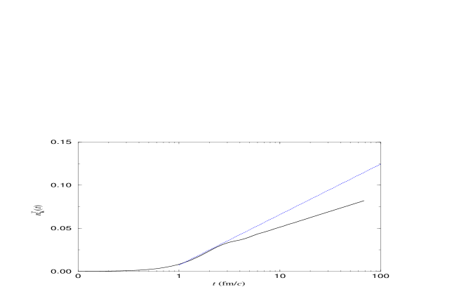
FIG. 3.: Off-shell contribution to $n^{\gamma}_{\bf k}(t)$ vs $t$ for hard photons $k\sim T$, $T=200\;\mbox{ MeV}$ and $\alpha=1/137$. The solid line is the numerical evaluation using the full time dependent rates, the dashed line is the HTL approximation.

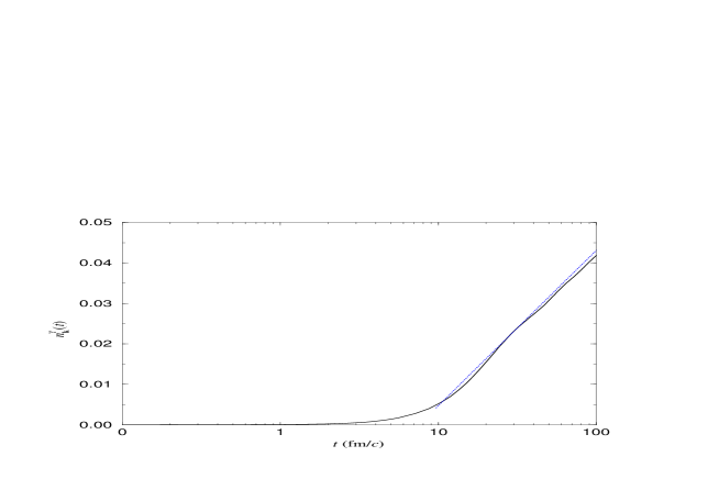
FIG. 4.: The number of semihard photons is plotted as a function of time for $e=0.01$, $T=200\;\mbox{MeV}$ and $eT/k=0.1$. The solid line is the numerical evaluation using the full time dependent rates, the dashed line is the HTL approximation.

FIG. 5.: The ratio of the number of hard photons produced by off-shell process ($q\rightarrow q\gamma$ and $\bar{q}\rightarrow\bar{q}\gamma$) to that produced by on-shell processes ($qg\rightarrow q\gamma$ and $q\bar{q}\rightarrow g\gamma$) as a function of QGP lifetime $t$ for $\alpha=1/137$, $\alpha_{s}=0.4$ and $T=200\;{\rm MeV}$.

REFERENCES

• [1] J. W. Harris and B. Muller, Annu. Rev. Nucl. Part. Sci. 46, 71 (1996); B. Muller in Particle Production in Highly Excited Matter, edited by H. H. Gutbrod and J. Rafelski, NATO ASI series B, Vol. 303 (Plenum, New York, 1993); H. Elze and U. Heinz, Phys. Rep. 183, 81 (1989); H. Meyer-Ortmanns, Rev. Mod. Phys. 68, 473 (1996); H. Satz, in Particle Production in Highly Excited Matter, edited by H.H. Gutbrod and J. Rafelski, NATO ASI series B, Vol. 303 (Plenum, New York, 1993).
• [2] B. Muller, The Physics of the Quark-Gluon Plasma, Lecture Notes in Physics, Vol. 225 (Springer-Verlag, Berlin, 1985); L. P. Csernai, Introduction to Relativistic Heavy Ion Collisions (John Wiley and Sons, England, 1994); C. Y. Wong, Introduction to High-Energy Heavy Ion Collisions (World Scientific, Singapore, 1994).
• [3] For a summary of recent results from SPS, see the CERN web page at http://www.cern.ch/CERN/Announcements/2000/NewStateMatter/; U. Heinz and M. Jacob, Evidence for a New State of Matter: An Assessment of the Results from the CERN Lead Beam Programme, nucl-th/0002042.
• [4] K. Geiger, Phys. Rep. 258, 237 (1995); Phys. Rev. D52, 1500 (1995); Phys.Rev. D54, 949 (1995); Ultrarelativistic nuclear collisions in a QCD based space-time description: the parton cascade model in Quark Gluon Plasma 2, Ed. by R. C. Hwa, (World Scientific, Singapore, 1995).
• [5] K. J. Eskola and X.-N. Wang, Phys. Rev. D49 1284 (1994), K. J. Eskola, B. Müller and X.-N. Wang, Phys. Lett. B374, 20 (1996); T. S. Biro et. al., Phys. Rev. C 48, 1275 (1993); T. S. Biro, B. Müller and X.-N. Wang, Phys. Lett. B283, 171, (1992).
• [6] E. Braaten and R.D. Pisarski, Nucl. Phys. B337, 569 (1990); ibid. B339, 310 (1990).
• [7] R.D. Pisarski, Physica A 158, 146 (1989); Phys. Rev. Lett. 63, 1129 (1989); Nucl. Phys. A525, 175 (1991).
• [8] R.D. Pisarski, Nucl. Phys. B309, 476 (1988).
• [9] H. A. Weldon, Phys. Rev. D 26, 1394 (1982); ibid. 2789 (1982); Phys. Rev. D 40, 2410 (1989); Physica A 158, 169 (1989).
• [10] R.D. Pisarski, Phys. Rev. Lett. 63, 1129 (1989); Phys. Rev. D 47,5589 (1993).
• [11] M. Le Bellac, Thermal Field Theory (Cambridge University Press, 1996).
• [12] H. A. Weldon, Phys. Rev. D28, 2007 (1983); Ann. of Phys. (N.Y.) 228, 43 (1993); J.-P. Blaizot in Proceedings of the Fourth Summer School and Symposium on Nuclear Physics, Eds. D. P. Min and M. Rho (World Scientific, Singapore, 1991).
• [13] L. S. Brown and L. G. Yaffe, Effective Field Theory for Highly Ionized Plasmas, physics/9911055.
• [14] J.-P. Blaizot and E. Iancu, Nucl. Phys. B459 559 (1996).
• [15] J. Schwinger, J. Math. Phys. 2, 407 (1961), K. T. Mahanthappa, Phys. Rev. 126, 329 (1962); P. M. Bakshi and K.T. Mahanthappa, J. Math. Phys. 41, 12 (1963), L. V. Keldysh, JETP 20, 1018 (1965), L. P. Kadanoff and G. Baym, Quantum Statistical Mechanics, (W. A. Benjamin, New York, 1962), K.-C. Chou, Z.-B. Su, B.-L. Hao, and L. Yu, Phys. Rep. 118, 1 (1985).
• [16] D. Boyanovsky, H.J. de Vega and R. Holman, in Proceedings of the Second Paris Cosmology Colloquium, Observatoire de Paris, 1994, edited by H.J. de Vega and N. Sánchez (World Scientific, Singapore 1995), pp. 127-215; in Advances in Astrofundamental Physics, Erice Chalonge School, edited by N. Sánchez and A. Zichichi (World Scientific, Singapore 1995); D. Boyanovsky, H. J. de Vega, R. Holman, D.-S. Lee and A. Singh, Phys. Rev. D 51, 4419 (1995); D. Boyanovsky, H. J. de Vega, R. Holman and J. Salgado, Phys. Rev. D 54, 7570 (1996).
• [17] D. Boyanovsky, H. J. de Vega and R. Holman, in Current Topics in Astrofundamental Physics, Vth Erice Chalonge School, edited by N. Sánchez and A. Zichichi (World Scientific, Singapore 1996), pp. 183-270; D. Boyanovsky, H. J. de Vega, R. Holman and D.-S. Lee, Phys. Rev. D 52, 6805 (1995); D. Boyanovsky, M. D’Attanasio, H. J. de Vega and R. Holman, Phys. Rev. D 54, 1748 (1996).
• [18] L. McLerran and T. Toimela, Phys. Rev. D31, 545, (1985); P. V. Ruuskanen, Photons and lepton pairs–the deep probes of the quark-gluon plasma, in Particle Production in Highly Excited Matter, Ed. Gutbrod, (Plenum, N.Y. 1993); Nucl. Phys. A544, 169c (1995).
• [19] J. Kapusta, P. Lichard and D. Seibert, Phys. Rev. D 44, 2774 (1991).
• [20] R. Baier, M. Dirks, K. Redlich and D. Schiff, Phys. Rev. D 56, 2548 (1997); R. Baier, H. Nakkagawa, A. Niegawa and K. Redlich, Z. Phys. C 53, 433 (1992); R. Baier, B. Pire and D. Schiff, Phys. Rev. D 38, 2814 (1988).
• [21] D. Boyanovsky, H. J. de Vega, R. Holman, and M. Simionato, Phys. Rev. D 60, 065003 (1999); D. Boyanovsky and H. J. de Vega, Phys. Rev. D 59, 105019 (1999).
• [22] D. Boyanovsky, H.J. de Vega, and S.-Y. Wang, Phys. Rev. D 61, 065006 (2000).
• [23] D. Boyanovsky, H. J. de Vega, R. Holman, S. P. Kumar, and R. D. Pisarski, Phys. Rev. D58, 125009 (1998).
• [24] A. Rajantie and M. Hindmarsh, Phys. Rev.  D 60, 096001 (1999).
• [25] J.-P. Blaizot and E. Iancu, Phys. Rev. Lett. 76, 3080 (1996); Phys. Rev. D 55, 973 (1997); Phys. Rev. D 56, 7877 (1997).
• [26] K. Takashiba, Int. J. Mod. Phys A 11, 2309 (1996).
• [27] D. Bodeker, Nucl.Phys. B566, 402 (2000).
• [28] D. F. Litim and C. Manuel, Nucl. Phys. B562, 237 (1999).
• [29] J.-P. Blaizot and E. Iancu, Nucl. Phys. B557, 183 (1999); Nucl. Phys. B570, 326 (2000).
• [30] D. Boyanovsky, D. Brahm, R. Holman and D.-S. Lee, Phys. Rev. D54, 1763 (1996).
• [31] S.-Y. Wang, D. Boyanovsky, H. J. de Vega, D.-S. Lee, and Y. J. Ng, Phys. Rev. D 61, 065004 (2000).
• [32] D. Boyanovsky, H. J. de Vega, D.-S. Lee, Y. J. Ng, and S.-Y. Wang, Phys. Rev. D 59, 105001 (1999).
• [33] J. Baacke, D. Boyanovsky, and H. J. de Vega, hep-ph/9907337.
• [34] L.-Y. Chen, N. Goldenfeld and Y. Oono, Phys. Rev. Lett. 73, 1311 (1994); Phys. Rev. E 54, 376 (1996); T. Kunihiro, Prog. Theor. Phys. 95, 503 (1995); ibid. 97, 179 (1997); S.-I. Ei, K. Fujii and T. Kunihiro, hep-th/9905088; H. J. de Vega and J. F. J. Salgado, Phys. Rev. D 56 6524, (1997); T. Kunihiro, Prog. Theor. Phys. Suppl. 131, 459 (1998); S.-I. Ei, K. Fujii and T. Kunihiro, Ann. of Phys. (N.Y.) 280, 236 (2000); M. Frasca, Phys. Rev. A 56, 1549 (1997); I. L. Egusquiza and M. A. Valle Basagoiti, Phys. Rev. D57, 1586 (1998); C. M. Bender and L. M. A. Bettencourt, Phys. Rev. Lett. 77, 4114 (1996), Phys. Rev. D54, 7710 (1996).
• [35] H.-T. Elze and U. Heinz, in Quark-Gluon Plasma edited by R.C. Hwa (World Scientific, Singapore, 1990); H.-T. Elze and U. Heinz, Phys. Rep. 183, 81 (1989).
• [36] S. Mrówczyński, in Quark-Gluon Plasma [35]; S. Mrówczyński and P. Danielewicz, Nucl. Phys. B342, 345 (1990); S. Mrówczyński and U. Heinz, Ann. Phys. (N.Y.) 229, 1 (1994); S. Mrówczyński, hep-ph/9805435.
• [37] P. Danielewicz, Ann. Phys. (N.Y.) 152, 239 (1984).
• [38] A. Niegawa, Prog. Theor. Phys. 102, 1 (1999), and references therein.
Refer to caption