Charm Production in Deep Inelastic Scattering
from Threshold to High $Q^{2}$

J. Amundson^a,b, C. Schmidt^a, W.K. Tung^a,b,c and X.N. Wang^a

^a Michigan State University, East Lansing, Michigan 48824, USA

^b Fermi National Laboratory, Batavia, IL 60510, USA

^c CERN, CH-1211 Geneva 23, Switzerland

Charm final states in deep inelastic scattering constitute $\sim 25\%$ of the inclusive cross-section at small $x$ as measured at HERA. These data can reveal important information on the charm and gluon structure of the nucleon if they are interpreted in a consistent perturbative QCD framework which is valid over the entire energy range from threshold to the high energy limit. We describe in detail how this can be carried out order-by-order in PQCD in the generalized $\overline{{\rm MS}}$ formalism of Collins (generally known as the ACOT approach), and demonstrate the inherent smooth transition from the 3-flavor to the 4-flavor scheme in a complete order $\alpha_{s}$ calculation, using a Monte Carlo implementation of this formalism. This calculation is accurate to the same order as the conventional NLO $F_{2}$ calculation in the limit $\frac{Q}{m_{c}}>>1$. It includes the resummed large logarithm contributions of the 3-flavor scheme (generally known in this context as the fixed-flavor-number or FFN scheme) to all orders of $\alpha_{s}\ln(m_{c}^{2}/Q^{2})$. For the inclusive structure function, comparison with recent HERA data and the existing FFN calculation reveals that the relatively simple order-$\alpha_{s}$ (NLO) 4-flavor ($m_{c}\neq 0$) calculation can, in practice, be extended to rather low energy scales, yielding good agreement with data over the full measured $Q^{2}$ range. The Monte Carlo implementation also allows the calculation of differential distributions with relevant kinematic cuts. Comparisons with available HERA data show qualitative agreement; however, they also indicate the need to extend the calculation to the next order to obtain better description of the differential distributions.

1 Introduction

Recent measurements of charm production in deep inelastic scattering (DIS) at HERA [1, 2] have shown that up to 25% of the total cross-section at small-x contains charm in the final state. This is within the expectations of perturbative QCD based on conventional parton distributions. We are now in a position to utilize this process to study details of the production mechanism of heavy quarks in general, and to extract useful information on the charm and gluon structure of the proton in particular.

Conventional perturbative QCD (PQCD) theory is formulated in terms of zero-mass quark-partons. For processes depending on one hard scale $Q,$ the well-known factorization theorem then provides a straightforward procedure for order-by-order perturbative calculations, as well as an associated intuitive parton picture interpretation of the perturbation series. Heavy quark production presents a challenge in PQCD because the heavy quark mass, $m{H}$ $(H=c,b,t),$ provides an additional hard scale which complicates the situation – it requires a different organization of the perturbative series depending on the relative magnitudes of $m{H}$ and $Q$.

The two standard methods for PQCD calculation of heavy quark processes represent two diametrically opposite ways of reducing the two-scale problem to a one-scale problem. (i) In the conventional parton model approach used in many global QCD analyses of parton distributions [3, 4, 5] and Monte Carlo programs, the zero-mass parton approximation is applied to a heavy quark calculation as soon as the typical energy scale of the physical process $Q$ is above the mass threshold $m{H}$. This leaves $Q$ as the only apparent hard scale in the problem. (ii) In the heavy quark approach which played a dominant role in “NLO calculations” of the production of heavy quarks [6, 7, 8], the quark $H$ is always treated as a “heavy” particle and never as a parton. The mass parameter $m{H}$ is explicitly kept along with $Q$ as if they are of the same order, irrespective of their real relative magnitudes.

The co-existence of these two opposite approaches represents an uneasy dichotomy in the current literature. On physical grounds, the zero-mass parton picture of heavy quarks should be applicable at energy scales very much larger than the relevant quark mass, $m{H}$ $\ll$ $Q$, whereas the heavy quark approach (often referred to as the fixed-flavor-number (FFN) scheme) should be more appropriate at energy scales comparable to the quark mass $m{H}$ $\sim$ $Q$. The actual experimental regime often lies in between these two extreme regions, where the validity of either approach can be called into question. There is, however, a natural way to incorporate both approaches in a unified framework in PQCD which provides a smooth transition between the two. This has been formulated in a series of papers over the years, Refs. [9, 10, 11, 12, 13], which has now been adopted, in different guises, by most recent literature on heavy quark production in PQCD. [15, 16, 17, 18]

To see the basic ideas behind this unified picture, let us focus explicitly on the production of charm ($H=c$) in deep inelastic scattering. All considerations apply to a generic heavy quark. Consider the PQCD calculation of the $F{2}(x,Q)$ structure function which receives substantial contribution from charm production as mentioned earlier. The underlying physical ideas are illustrated graphically in Fig. 1 where the charm contribution to this structure function, denoted $F{2}^{c}(x,Q)$, is plotted as a function of $Q$ at some fixed value of $x$.

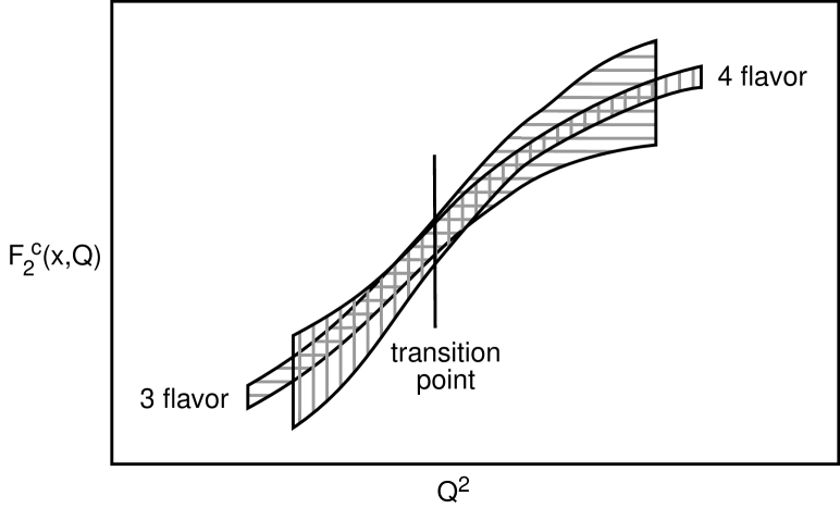
Figure 1: Schematic illustration of the uncertainty bands (hence the relative merits) of the 3-flavor and 4-flavor scheme calculations of the charm contribution to the inclusive structure function – and how they can be naturally merged into a composite scheme.

Near threshold $Q\sim m{c}$, it is natural to consider the charm quark as a heavy particle, and to adopt the 3 active-parton-flavor scheme of calculation (the “heavy quark approach”). As $Q$ becomes large compared to $m{c}$, the fixed-order calculation in this approach becomes unreliable since the perturbative expansion contains terms of the form $\alpha{s}^{n}\log^{n}\left(m{c}^{2}/Q^{2}\right)$ at any order $n$, which ruin the convergence of the series—these terms are not infra-red safe as $m{c}$ $\rightarrow 0$ or $Q\rightarrow\infty$. Thus the uncertainty of the 3-flavor calculation grows as $Q/m{c}$ becomes large. This is illustrated in Fig. 1 as an error band marked by horizontal hashes which is narrow near threshold but becomes ever wider as $Q/m{c}$ increases. On the other hand, starting from the high energy end ($Q\gg m{c}$), the most natural calculational scheme to adopt is the conventional 4-flavor scheme with active charm partons. (In this approach, the infra-red unsafe large logarithms mentioned earlier are “resummed” and absorbed into the finite charm parton distributions.) However, as we go down the energy scale toward the charm production threshold region, the 4-flavor calculation becomes unreliable because the approximation $m{c}=0$ deteriorates as $Q\rightarrow m{c}$. The uncertainty band of such a calculation is outlined in Fig. 1 by the vertical hashes – it is narrow at high energies, but becomes increasingly wider as one approaches the threshold region.

The intuitive ideas embodied in Fig 1 illustrate that: (i) these two conventional approaches are individually unsatisfactory over the full energy range, but are mutually complementary; and (ii) the most reliable PQCD prediction for the physical $F{2}(x,Q)$, at a given order of calculation, can be obtained by utilizing the most appropriate scheme at that energy scale $Q$, resulting in a composite scheme, as represented by the cross-hashed region in Fig. 1. The use of a composite scheme consisting of different numbers of flavors in different energy ranges, rather than a fixed number of flavors, is familiar in the conventional zero-mass parton picture. The new formalism espoused in Refs. [9, 10, 11, 12] provides a quantum field theoretical basis [19, 13] for this intuitive picture in the presence of non-zero quark mass.

This generalization brings about several important distinguishing features and insights. First, after the hard cross-section is rendered infra-red safe by factorizing out the $\ln(m{c})$ terms, the remaining finite dependence on $m{c}$ can be kept in the hard cross-sections to maintain better accuracy in the intermediate energy region.One can then show that the unified formalism reproduces the two conventional approaches in well-defined ways in their respective regions of applicability [9]-[13]. Secondly, it has become clear recently that there is much inherent flexibility in the choice of the transition energy scale (cf. Fig. 1) as well as the detailed matching condition between the 3- and 4-flavor calculations. This makes it possible to have a variety of different implementations of the new formalism [15, 16, 17, 18], with different emphases. Properly understood, this feature can be exploited to lend strength to the formalism; but, during the development of the theory, the subtleties have given rise to much misunderstanding and confusion in existing literature.

In this paper, we study charm production in DIS using the general mass formalism, and compare the results with recent HERA data. The main goals of this work are:

• (i) Through this specific example, we give a concise and careful presentation of the general formalism, including the relatively simple operational procedure for calculating its various components at any order of $\alpha_{s}$. We hope this will help fill the gap between the original, relatively sketchy, ACOT paper [12] and the recent, more technical, all-order proof of the formalism by Collins [13].

• (ii) We carry out the numerical calculations to make concrete the intuitive ideas illustrated in Fig. 1; and to demonstrate the validity of the physical principles underlying the composite scheme.

• (iii) We show that the flexibility of the general formalism mentioned above can result in efficient PQCD calculations of inclusive quantities at relatively low order in $\alpha_{s}$ compared to FFN calculations – because the relevant physics has been effectively “resummed” by the appropriate scheme adopted for the given energy scale.

Item (i) is basic; it forms the foundation for the other two parts. However, since this part is about the clarification of the existing theoretical formalism rather than new work, and since not all readers are concerned with theoretical precision, we have elected to place it in the Appendix. Hopefully, this will increase the accessibility of the main body of the paper. In regards to the underlying physics, we believe the discussion in the appendix should make a useful contribution to clear the confusion and misunderstanding among the various approaches that have been proposed in the recent literature following [12].

Based on the terminologies discussed in this Appendix, in Sec. 2 we describe the complete order $\alpha_{s}$ calculation carried out in this paper in relation to previous work on this subject. The new calculation extends the validity of the original ACOT results to NLO in the high energy regime – on the same level as the conventional zero-mass total inclusive structure functions. In addition, the new perspective, as illustrated in Fig. 1 above and discussed quantitatively in the paper proper, allows a re-assessment of the physical predictions of the order $\alpha_{s}$ calculation near the threshold region, making it a viable alternative to the order $\alpha_{s}^{2}$ FFN calculation. In Sec. 3 we present the numerical results on inclusive charm production, and demonstrate that the validity and the efficiency of the general formalism, as described in (ii) and (iii) above, are indeed seen at this order. We show that very good agreement with recent HERA data on inclusive $F{2}^{c}$ is obtained in practice. For this study, we have developed a new implementation of the generalized $\overline{{\rm MS}}$ formalism using Monte Carlo methods. This implementation allows the computation of differential distributions, with kinematic cuts, such as $d\sigma^{D^{\ast}}/dp{t},\;d\sigma^{D^{\ast}}/dQ,$ and $d\sigma^{D^{\ast}}/d\eta$ which we present in Sec. 4. These results, are in qualitative agreement with available data from HERA. However, they are not as good as those of the order $\alpha{s}^{2}$ calculation in the 3-flavor scheme. This is to be expected for differential distributions with experimental cuts, since the (resummed) low-order calculation contains more severe approximations to the kinematics of the final state partons. For future quantitative studies, the general formalism needs to be expanded to incorporate higher-order results (adaptable from existing FFN calculations). This point is discussed in the concluding section, along with other observations.

2 Total Inclusive Structure Functions in the general formalism

We consider the inclusive DIS structure functions, such as $F_{2}$, focusing on the contribution of a massive quark. For definiteness, we assume that the only relevant quark with non-zero mass is the charm quark. The generic leptoproduction process is depicted in Fig. 2:

$$\ell_{1}+A\longrightarrow\ell_{2}+X,$$ (1)

where $A$ is a hadron, $\ell_{1,2}$ are leptons, and $X$ represents the summed-over final state hadronic particles. Note that $X$ may or may not contain a visible heavy-flavor hadron.

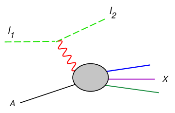
Figure 2: The generic inclusive lepto-production process. We are primarily interesting in final states which contain some heavy quarks, in particular charm.

After the calculable leptonic part of the cross-section has been factored out, we work with the hadronic process induced by the virtual vector boson $\gamma^{\ast}$ of momentum $q$ and polarization $\lambda$:

$$\gamma^{\ast}(q,\lambda)+A(P)\longrightarrow X(P_{X}).$$ (2)

Although our considerations apply to DIS processes induced by $W$ and $Z$ as well, we shall explicitly refer to the neutral current interaction with the exchange of a virtual photon $\gamma^{\ast}$ in order to be concrete. The cross-section is expressed in terms of the hadronic tensor

$$W_{\lambda\sigma}(q,P)=\frac{1}{4\pi}\mathrel{\mathop{\overline{\sum}}\limits_{X(P_{X}),spin}}\langle P|e_{\lambda}^{\ast}\cdot J^{\dagger}|P_{X}\rangle(2\pi)^{4}{\delta^{(4)}\left(P+q-P_{X}\right)}\langle P_{X}|e_{\sigma}\cdot J|P\rangle.$$ (3)

where $\overline{{\sum}}$ denotes a sum over all final hadronic states. In most cases, it suffices to consider the diagonal elements of the tensor $F^{\lambda}\equiv W_{\lambda\lambda}(q,P).$

The factorization theorem in the presence of non-zero quark masses – assumed in [12] and established to all orders in PQCD [13] – states that the inclusive cross-section can be written as a convolution:

$$F_{A}^{\lambda}(Q^{2},x,..)=\mathrel{\mathop{\sum}\limits_{a}}f_{A}^{a}(x,\mu)\otimes\widehat{\omega}_{a,\lambda}(x,Q/\mu,Q/m_{c},\alpha_{s}\left(\mu\right))\;+\;\mathcal{O}\Bigl{(}\Lambda/Q\Bigr{)}^{p}$$ (4)

where $f_{A}^{a}$ is the distribution of parton $a$ inside the hadron $A$, $\widehat{\omega}_{a,\lambda}$ is the perturbatively calculable hard cross-section for $\gamma^{\ast}+a\rightarrow X$, $p$ is some positive number, $\mu$ denotes collectively the renormalization and factorization scales, and a convolution in the $x$ variable is implied. The helicity structure functions $F^{\lambda}$ are simply related to the familiar $F_{1,2,3}$ [11].

The exact way that the physical structure function factorizes into the long-distance ($f_{A}^{a}$) and the short-distance ($\widehat{\omega}_{a,\lambda}$) pieces on the right-hand side of Eq. (4) depends on the scheme used to define the parton distributions. The physical structure function $F_{A}^{\lambda}$ should be independent of any calculational scheme; therefore, the definition of the hard cross-sections is determined by the subtraction procedure used to define the parton distributions. As discussed in the Introduction, the general formalism consists of the 3-flavor scheme at low energy scales, the 4-flavor scheme at high energy scales, and a suitably chosen transition region where matching conditions between the two schemes are applied. The precise description of these elements of the formalism is given in the Appendix. Operational definitions of quantities needed in subsequent discussions are also discussed in some detail there.

2.1 Previous calculations

To put the current calculation in context, we first summarize the existing calculations of leptoproduction of charm using the precise definitions given in the Appendix.

• NLO 3-flavor (3$\alpha_{s}^{2}$) calculation [7]: Most dedicated calculations of heavy flavor production in recent years have been carried out in this scheme. The LO process is $\mathcal{O}(\alpha_{s}^{1})$ heavy-flavor creation (HC), $\gamma^{\ast}g\rightarrow c\bar{c}$. The NLO processes consist of the $\mathcal{O}(\alpha_{s}^{2})$ virtual corrections to $\gamma^{\ast}g\rightarrow c\bar{c}$ as well as the real HC $\gamma^{\ast}l\rightarrow c\bar{c}l$ process, where $l$ denotes any light parton. Cf. Fig. 3. This calculation becomes questionable when $Q\gg m_{c}$ – i.e., it ceases to be “NLO” in accuracy, as indicated in Fig. 1, because the perturbative expansion is actually in $\alpha_{s}ln(Q^{2}/m_{c}^{2})$ for large $Q$.

  

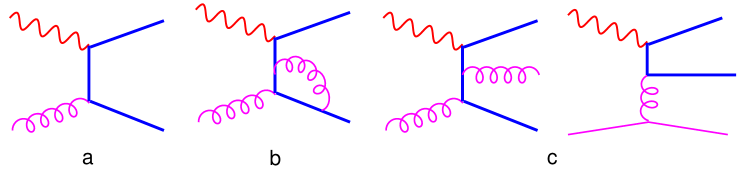
  Figure 3: Representative Feynman diagrams contributing to the calculation of the partonic structure functions for charm production in the 3-flavor scheme due to: (a) order $\alpha_{s}^{1}$ heavy-flavor creation (HC) or gluon fusion mechanism; (b) order $\alpha_{s}^{2}$ virtual correction to (a); and (c) order $\alpha_{s}^{2}$ real corrections involving gluon and light-quark initial states.

• Zero-mass 4-flavor (ZM) (4$\alpha_{s}^{1};$ $m_{c}=0$) calculation: This is the formalism used in most conventional QCD parton model calculations and popular Monte Carlo programs. It represents an approximation to the general mass (GM) 4-flavor scheme by setting $m_{c}=0$ in the hard cross-sections $\hat{\omega}_{a}(x,\frac{Q}{\mu},\frac{m_{c}}{Q},\mu)\stackrel{{\scriptstyle m_{c}/Q\rightarrow 0}}{{\longrightarrow}}\hat{\omega}_{a}^{m_{c}=0}(x,\frac{Q}{\mu},\mu).$ The LO contribution consists of the $\mathcal{O}(\alpha_{s}^{0})$ $\gamma^{\ast}c\rightarrow c$ heavy-flavor excitation (HE) process. The NLO contribution consists of the $\mathcal{O}(\alpha_{s}^{1})$ virtual corrections to $\gamma^{\ast}c\rightarrow c$ plus the real HC $\gamma^{\ast}g\rightarrow c\bar{c}$ and, $\gamma^{\ast}c\rightarrow gc$ HE processes. Cf. Fig. 4. This calculation is unreliable in the threshold region, as mentioned in the introduction.

  

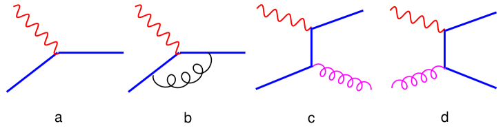
  Figure 4: Representative Feynman diagrams contributing to the calculation of the partonic structure functions for charm production in the 4-flavor scheme due to: (a) order $\alpha_{s}^{0}$ heavy-flavor excitation (HE) mechanism; (b) order $\alpha_{s}^{1}$ virtual correction to (a); (c) order $\alpha_{s}^{1}$ real corrections to the HE mechanism; and (d) order $\alpha_{s}^{1}$ heavy-flavor creation mechanism.

• LO generalized $\overline{{\rm MS}}$ calculation (ACOT) [12]: This represents the simplest implementation of the generalized formalism [12]. It emphasizes the overlapping physics underlying the 3-flavor and 4-flavor calculations in the region not far above threshold. The 4-flavor calculation consists of HE $\gamma^{\ast}c\rightarrow c$ (Fig. 4a) plus $m_{c}\neq 0$ HC $\gamma^{\ast}g\rightarrow c\bar{c}$ (Fig. 4d), with the requisite subtraction term which removes the $m_{c}$ mass-logarithm. Mathematically, the result on $F_{2}(x,Q,\mu)$ can be shown to match that of the $\mathcal{O}(\alpha_{s}^{1})$ 3-flavor scheme calculation (HC $\gamma^{\ast}g\rightarrow c\bar{c}$) as the (unphysical) factorization scale $\mu$ approaches $m_{c}$ from above [12]. Physically, the predicted behavior of $F_{2}^{c}$ for $Q\sim m_{c}$ will depend on the choice of $\mu$ as a function of the physical variables, cf. next section. At a high energy scale, $\mu\sim Q\gg m_{c}$, this calculation only approximates the 4-flavor NLO results: it contains the most important $\mathcal{O}(\alpha_{s}^{1})$ term, HC $\gamma^{\ast}g\rightarrow c\bar{c}$ (because of the large gluon distribution and the need for matching), but does not include the smaller $\mathcal{O}(\alpha_{s}^{1})$ terms represented by Fig. 4b,c. This calculation has been further studied by Kretzer and Schienbein [21] and Krämer et al [22].

• Variations on the “variable flavor number” theme: In recent years, the general approach proposed in [9, 12] has been adopted by other groups, starting from different historical perspectives, [15, 16, 17, 18]. In contrast to the fixed flavor-number (FFN) approach, these are usually referred to as being in the variable flavor-number (VFN) scheme. This terminology has caused some confusion, since although the common theme is that of [9, 12], as shown in Fig. 1, the various implementations differ considerably. Whether a particular implementation is self-consistent within the general framework of PQCD, or whether two implementations are compatible within the accuracy of the perturbative expansion, are often unclear or controversial (e.g. [23]) because of the complexity of the multi-scale problem and because of possible misunderstandings. It is beyond the scope of this paper to critically review these approaches. By pursuing the goals described in the introduction, we hope to provide a clearer picture of the general formalism of [13], hence a better basis to help address some of the controversial issues in the future.

2.2 The full order $\alpha_{s}$ generalized $\overline{{\rm MS}}$ calculation

The calculation of charm contribution to the inclusive structure functions reported in this paper completes the order $\alpha_{s}$ calculation in the general formalism, initiated in [12], including all the hard processes of Fig. 4. The additional terms, although relatively small numerically at current energies, are required to make the 4-flavor part of this calculation truly NLO at high energies, so that it becomes equivalent to the conventional zero-mass NLO theory used in most modern analyses of precision DIS data. In the remainder of this section we discuss the theoretical issues and uncertainties in the order $\alpha_{s}$ 4-flavor calculation at all energy scales, in order to address the issues highlighted at the end of the introduction, Sec. 1.

At order $\alpha_{s}^{1}$ the 3-flavor component of the composite scheme consists of only the (unsubtracted) $\mathcal{O}(\alpha_{s}^{1})$ HC $\gamma^{\ast}g\rightarrow c\bar{c}$ process. The result is standard. Therefore, our main calculation concerns the 4-flavor scheme component. At order $\alpha_{s}^{1}$ the right-hand side of Eq. (4) consists of three terms

$$\begin{array}[]{lll}F^{(4)}_{A,\lambda}(Q^{2},x,m_{c},\mu)&=&\;\;\;f_{A}^{c}\otimes\,^{0}\widehat{\omega}_{c,\lambda}^{c}\\ &&+\;f_{A}^{g}\otimes\,^{1}\widehat{\omega}_{g,\lambda}^{c\bar{c}}\\ &&+\;f_{A}^{c}\otimes\,^{1}\widehat{\omega}_{c,\lambda}^{cX}\\ &&+\;{\rm light-parton\ contributions}\ ,\end{array}$$ (5)

where the superscript (4) indicates that this is a 4-flavor calculation, and the hard-scattering cross-sections ${}^{i}\widehat{\omega}_{a,\lambda}^{X}$ for the various subprocesses are calculated from the corresponding partonic cross-sections ${}^{i}\omega_{a,\lambda}^{X}$ (without the hat) according to the procedures described in the Appendix. A description of each of the terms follows:

• The leading order $\gamma^{*}c\rightarrow c$ (Fig. 4a) partonic cross-section ${}^{0}\omega_{c,\lambda}^{c}$ is infra-red safe, thus

  $${}^{0}\widehat{\omega}_{c,\lambda}^{c}=\,^{0}\omega_{c,\lambda}^{c}\ .$$ (6)

• The $\gamma^{*}g\rightarrow c\bar{c}$ (Fig. 4d) partonic cross-section contains a single power of $\ln\mu^{2}/m_{c}^{2}$ which can be factorized into the charm distribution function by the subtraction [12]

  $${}^{1}\widehat{\omega}_{g,\lambda}^{c\bar{c}}=\,^{1}\omega_{g,\lambda}^{c\bar{c}}-\,^{1}\tilde{f}_{g}^{c}\otimes\,^{0}\omega_{c,\lambda}^{c}\ ,$$ (7)

  where the cancelling logarithm with mass-singularity resides in the $\mathcal{O}(\alpha_{s})$ perturbative parton distribution function

  $${}^{1}\tilde{f}_{g}^{c}=(\alpha_{s}/2\pi)P_{g\rightarrow q}(x)\ln(\mu^{2}/m_{c}^{2})$$ (8)

• The virtual correction to $\gamma^{*}c\rightarrow c$ (Fig. 4b) plus the real $\gamma^{*}c\rightarrow gc$ (Fig. 4c) partonic process also contain $\ln\left(\mu^{2}/m_{c}^{2}\right)$ terms which are factorized into the charm distribution function by the subtraction

  $${}^{1}\widehat{\omega}_{c,\lambda}^{cX}=\,^{1}\omega_{c,\lambda}^{cX}-\,^{1}\tilde{f}_{c}^{c}\otimes\,^{0}\omega_{c,\lambda}^{c}\ ,$$ (9)

  where the logarithm appears in the $\mathcal{O}(\alpha_{s}^{1})$ perturbative parton distribution function

  $${}^{1}\tilde{f}_{c}^{c}={\frac{\alpha_{s}}{2\pi}}{\frac{4}{3}}\Biggl{[}\biggl{(}{\frac{1+x^{2}}{1-x}}\biggr{)}\biggl{(}\ln{\frac{\mu^{2}}{m_{c}^{2}}}-1-2\ln(1-x)\biggr{)}\Biggr{]}_{+}\ .$$ (10)

Substituting Eqs. (6)-(9) into Eq. (5), the right-hand side can be re-organized as

$$\begin{array}[]{lll}F^{(4)}_{A,\lambda}(Q^{2},x,m_{c},\mu)&=&\;\;f_{A}^{g}\otimes\,^{1}\omega_{g,\lambda}^{c\bar{c}}\\ &&+\,(f_{A}^{c}-\;f_{A}^{g}\otimes\,^{1}\tilde{f}_{g}^{c}-f_{A}^{c}\otimes\,^{1}\tilde{f}_{c}^{c})\,\otimes\,^{0}\omega_{c,\lambda}^{c}\\ &&+\;f_{A}^{c}\otimes\,^{1}\omega_{c,\lambda}^{cX}\\ &&+\;{\rm light-quark\ terms}\ ,\end{array}$$ (11)

where the $\ln\left(\mu/{m_{c}}\right)$ terms in the $\omega_{a,\lambda}$ factors are kept intact, and the needed subtraction terms are explicitly grouped with the leading 2$\rightarrow$1 term with the same kinematics. This is the form we use for the actual numerical calculations, which we implement using a Monte Carlo approach.

It is useful to compare this calculation with the NLO 3-flavor calculation [7] which can be written, in the same notation, as follows

$$\begin{array}[]{lll}F_{A,\lambda}^{(3)}(Q^{2},x,m_{c},\mu)&=&\;\;f_{A}^{g}\otimes\,^{1}\omega_{g,\lambda}^{c\bar{c}}\\ &&+\;f_{A}^{g}\otimes\,^{2}\omega_{g,\lambda}^{gc\bar{c}}\\ &&+\;f_{A}^{q}\otimes\,^{2}\omega_{q,\lambda}^{qc\bar{c}}\\ &&+\;{\rm light-quark\ terms}\end{array}\ .$$ (12)

The term common to the two schemes is $\mathcal{O}\left(\alpha_{s}^{1}\right)$ $\gamma^{\ast}g\rightarrow c\bar{c}$, which appears as the first line in both Eq. 11 and Eq. 12. For this comparison, one can consider the rest of the terms in these equations as complementary “corrections” to the first term. In particular, the last two terms in the 3-flavor formula Eq. 12 are genuine $\mathcal{O}\left(\alpha_{s}^{2}\right)$ corrections to the common term in the threshold region; hence are commonly referred to as NLO. But at high $Q^{2}\gg m_{c}^{2}$, these terms contain large logarithm factors $\ln{Q^{2}}/{m_{c}^{2}}$ which vitiates the perturbation expansion. They are not NLO in this region.

In the 4-flavor calculation as organized in the form Eq. 11, the last two lines are also effectively $\mathcal{O}\left(\alpha_{s}^{2}\right)$. This is because the distribution $f_{A}^{c}$ is effectively $\mathcal{O}\left(\alpha_{s}^{1}\right)$ near threshold, and there is a built-in cancellation between the leading order $\gamma^{\ast}c\rightarrow c$ partonic cross-section and the first subtraction term in Eq. 11, as discussed in detail in Ref.[12]. Although these $\mathcal{O}\left(\alpha_{s}^{2}\right)$ “correction” terms to the $\mathcal{O}\left(\alpha_{s}^{1}\right)$ common term (first line) do not contain the full NLO $\mathcal{O}\left(\alpha_{s}^{2}\right)$ corrections at threshold, they do contain all the $\mathcal{O}\left(\alpha_{s}^{2}\right)$ contributions which are enhanced by $\ln\left({Q^{2}}/{m_{c}^{2}}\right)$ and quickly dominate as $Q^{2}$ increases. In fact, these large logarithmic terms have been resummed to all orders in perturbation theory via the DGLAP-evolved charm parton distribution contributions in the second and third lines. Therefore, in the large $Q^{2}$ region the 4-flavor result represents a true NLO calculation.

In principle, if carried out to all orders in $\alpha_{s}$, the 3-flavor and 4-flavor calculations in the form of $F_{A,\lambda}^{(i)}(Q^{2},x,m_{c},\mu)$, $i=3,4$, would give exactly the same prediction for all values of the arguments. The dependence on the scheme $(i)$ and the scale $(\mu)$ arises from the truncation of the perturbation series. Therefore, in order to produce a physical prediction $F_{A,\lambda}^{phys}(Q^{2},x,m_{c})$ and to relate the predictions in the two schemes, a number of additional steps must be taken. In the presence of a non-zero heavy quark mass, some of these steps are non-obvious; hence they can be the source of confusion. An explicit discussion of these elements of the calculation will make clear the flexibility as well as the uncertainties inherent in the formalism. This we do in the Appendix, as part of the more precise description of the formalism. Here, we mention only two features which are particularly relevant for the subsequent discussions of physical predictions.

First, within each scheme ($i=3$ or $4$), one needs to specify $\mu$ as a function of the physical variables in order to make a physical prediction, i.e.

$$F_{A,\lambda}^{phys}(Q^{2},x,m_{c})=F_{A,\lambda}^{(i)}(Q^{2},x,m_{c},\mu(x,Q,m_{c}))$$

Although there is considerable freedom in choosing $\mu(x,Q,m_{c})$, two conditions should be met so that the prediction can be reliable: (i) $\mu$ must be of the order of $Q$ or $m_{c}$ so that PQCD applies, and (ii) $F_{A,\lambda}^{(i)}(Q^{2},x,m_{c},\mu)$ must be relatively stable with respect to variations of $\mu$ for the ($x,Q$)-range of interest. This is the well-known scale-dependence of any PQCD calculation. For the problem at hand, a common choice for $\mu(x,Q,m_{c})$ is $\sqrt{Q^{2}+m_{c}^{2}}$: it represents the typical virtuality of the internal parton lines in the important subprocesses. The presence of the uncertainty associated with the choice of $\mu(x,Q,m_{c})$ in each scheme is illustrated in Fig. 1 by the respective bands.

Secondly, as shown in Fig. 1, one needs to identify an appropriate scale at which the 3-flavor and the 4-flavor scheme predictions are both reasonable and mutually comparable, so that the transition from one to the other in the composite scheme can be made smoothly. In the next section we show that, for the inclusive charm production cross-section, these conditions can be met over a rather large range of $Q$, extending down to near the threshold region. One possibility then is to choose the transition point (cf. Fig. 1) at a low value, close to $m_{c}$, so that in effect the 4-flavor calculation by itself covers the full range of physical interest.

In existing literature, it is already known that the 3-flavor order $\alpha_{s}^{2}$ (NLO) calculation can be extended to most of the currently accessible energy scales without manifest ill-effects of the large logarithms; and it agrees with data rather well. Its efficacy at very large $Q$ is not fully tested (cf. [16] and results of next section). Our calculation will demonstrate the robustness of the complementary, much simpler (order $\alpha_{s}$) 4-flavor calculation. It is worthwhile pointing out that, in the 4-flavor scheme, the order $\alpha_{s}$ calculation is, in fact, also NLO – since the LO $\gamma^{*}c\rightarrow c$ term is of order $\alpha_{s}^{0}$, as is the case in the standard QCD theory of inclusive structure functions. This important point is discussed in detail in the Appendix, Sec. A.5.

3 Inclusive Charm Structure Function

In the previous section, the theoretical formulation of charm production in DIS is presented within the context of the totally inclusive structure functions $F_{\lambda}(x,Q)$. Although terms involving at least one charm quark in the final state are the main subject of discussion, they have been added to “light quark contributions” to form the totally inclusive structure functions, cf. Eqs. 11 and 12.  The reason to do this (rather than simply talk about an “inclusive charm structure function”, say $F_{2}^{c})$ is: charm quarks are not physically observable; there is no unique or obvious definition of a “$F_{2}^{c}$” either experimentally or theoretically. Any experimental definition necessarily depends on the procedure or prescription for tagging final state charm (analogous to the jet-algorithm for defining jets). Any theoretical definition will be scheme-dependent, and will be subjected to questions such as infra-red safety (IRS), e.g. free from $\ln(m_{c})$ terms. The proper matching of the experimental and theoretical definitions is also necessary for a meaningful comparison of theory with experiment.

In this section, we shall be concerned with the comparison of our calculation of inclusive charm production structure function with previous calculations, such as that of ACOT [12] and that of the NLO three-flavor scheme [7], as well as with existing experimental results. Since the energy range where these comparisons will be made is moderate, the question of infra-red safety is not a critical one – as evidenced by the general phenomenological success of the NLO 3-flavor calculation (which is not IRS in the sense used in this paper). For this purpose, it suffices to define the theoretical 4-flavor $F_{2}^{c}$ as the quantity consisting of terms with at least one charm quark in the final state in Eq. 11, i.e. it is the right-hand side less the light-quark contribution. At the order we are calculating, this $F_{2}^{c}$ is actually well-defined and infra-red safe, – there are no large logarithm terms. In addition, since the charm mass is just about at the scale for PQCD to become valid and, as discussed at the end of the previous section, the transition scale can in practice be chosen close to $m_{c}$, the generalized $\overline{{\rm MS}}$ calculation reduces in practice to a 4-flavor (general mass) calculation.

The 4-flavor NLO calculation:

The parton distribution functions $f_{A}^{a}(x,\mu)$ needed for this calculation must be defined in the same renormalization scheme as the hard cross-sections used. In the 4-flavor general mass calculation, most CTEQ parton distributions have been defined in the ACOT scheme as described in the Appendix, with the matching scales chosen at the heavy quark masses. In particular, the CTEQ5HQ set is generated with non-zero heavy quark masses in the hard cross-sections, hence it is the relevant one for our application. This set is evolved using NLO evolution, which is appropriate to our calculation which is NLO at high energies. For the numerical results presented below, we use an updated version of CTEQ5HQ [24]. In order to compare with results from the LO and NLO 3-flavor scheme, we need the corresponding parton distributions in the 3-flavor scheme. The CTEQ5F3 distributions satisfy this need, since they are obtained from global analysis of the same data sets as the CTEQ5HQ set, but with parton distributions and hard cross-sections in the 3-flavor scheme.

The calculation of the hard cross-section at $\mathcal{O}(\alpha_{s})$ is based on Eqs. 7 and 9. In the expression for the overall structure functions, the combination $f_{A}^{g}\otimes\,^{1}\omega_{g,\lambda}^{c\bar{c}}$ $+\,(f_{A}^{c}-\;f_{A}^{g}\otimes\,^{1}\tilde{f}_{g}^{c}$) $\otimes\,^{0}\omega_{c,\lambda}^{c},$ due to the subprocesses $\gamma^{\ast}c\rightarrow c$ and $\gamma^{\ast}g\rightarrow c\bar{c},$ comprise the original ACOT calculation [12]. With non-zero $m_{c},$ they are all finite. The implementation of these terms in the new Monte Carlo calculation is straightforward. We have verified that the new MC program reproduces the original ACOT results in detail. Illustrations of the relative contributions of the various terms can be found in Ref. [12]. Also, the smooth transition of the results of the general formalism from the 3-flavor one near threshold to the 4-flavor one at high energies is described in that paper.

The additional contributions $f_{A}^{c}\otimes\,^{1}\omega_{c,\lambda}^{cX}-f_{A}^{c}\otimes\,^{1}\tilde{f}_{c}^{c}\otimes\,^{0}\omega_{c,\lambda}^{c},$ due to the $\gamma^{\ast}c\rightarrow gc$ subprocess and virtual correction to the Born $\gamma^{\ast}c\rightarrow c$ term, are new for this calculation. They contain soft divergences which must be cancelled. In this Monte Carlo implementation, we use the phase-space splicing method to achieve the proper cancellation of the soft divergences between the real and virtual parts. Details of this calculation are contained in [25]. For double-checking, we have independently implemented an analytic calculation based on the formulas of Hoffmann and Moore [26]. The two calculations agree quite well with each other over the full phase space, with the exception of small values of $Q/m_{c}$. The difference could be attributed to a different treatment of the massive charm quark kinematics adopted by Ref. [26] in deriving their formulas. This effect goes away when $m_{c}$ is small compared to $Q,$ as expected.

Results and Comparison with order $\alpha_{s}^{2}$ 3-flavor calculation:

We now present some typical numerical results on the theoretical $F_{2}^{c}(x,Q)$ obtained in our order $\alpha_{s}$ 4-flavor calculation compared to those of order $\alpha_{s}^{2}$ 3-flavor scheme. The 3-flavor results were obtained from the parametrization of Ref. [27]. Each calculation corresponds to a different way of organizing the perturbation series, hence has its natural region of applicability, as discussed in the previous sections. To do a meaningful comparison, it is important to take into account the estimated uncertainties of each calculation. Following the example of Fig. 1, we plot a band for each of the predictions, obtained with two common choices of the renormalization and factorization scales: $\mu=c\sqrt{Q^{2}+m_{c}^{2}}$ with $c=0.5$ and $2.0$. (This choice is more natural than that of the original ACOT paper, c.f. footnote h.) The 3-flavor calculation requires parton distributions defined in the same scheme. We use the CTEQ5F3 set. The results vary in appearance, depending on the kinematic variables. Two representative plots relevant for the HERA measurements are shown in Fig. 5 where $F_{2}^{c}(x,Q)$ is plotted against $Q$ for two values of $x$: (a) $x=0.01;$ and (b) $x=0.0001.$ These constitute real examples of the cartoonistic Fig. 1, which is designed to emphasize the underlying ideas.

      

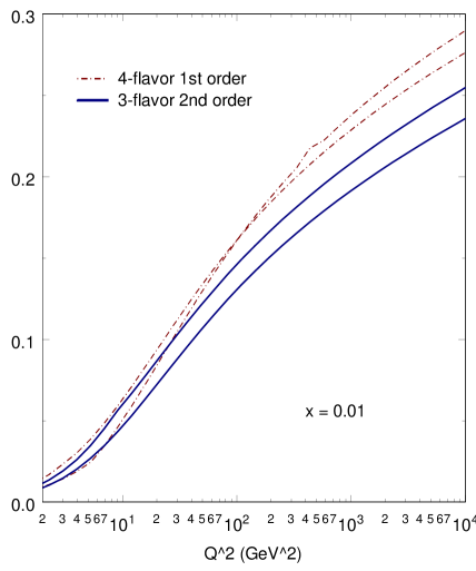
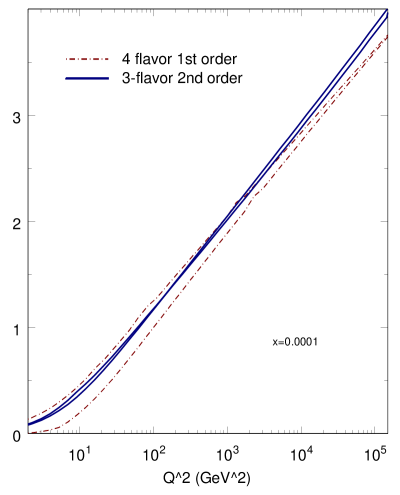
Figure 5: Comparison of results of the present order $\alpha_{s}$ generalized $\overline{{\rm MS}}$ 4-flavor calculation to that of order $\alpha_{s}^{2}$ 3-flavor calculations for: (a) $x=0.01$; and (b) $x=0.0001$. $F_{2}^{c}$ is plotted against $Q$. The uncertainties of the calculation are represented by a band bounded by two curves obtained with the scale choices $\mu=c\sqrt{Q^{2}+m_{c}^{2}}$; $c=0.5,2$.

These plots show that the overlapping region of the two schemes is quite wide for $x=10^{-4}$; and the overall behavior conforms with expectations. For $x=10^{-2}$, the overlapping region is more limited and it is confined to low $Q$ values. The 3-flavor results fall below the 4-flavor ones at large values of $Q$ where the latter should be more reliable. Compared to current data, both are within the experimental range; the 4-flavor results are closer to the data points, cf. next subsection, although the uncertainties of the 4-flavor calculation are fairly large for $x=10^{-4}$.

Since the order $\alpha_{s}$ 4-flavor results are comparable to the order $\alpha_{s}^{2}$ ones at energy scales close to the threshold in both cases (and for other values of $x$), it is reasonable to choose the transition scale at a relatively low value, as mentioned earlier in the paper. The band representing the 3-flavor calculation does become wider at large Q for $x=10^{-2}$ (where the absolute values also are lower than the 4-flavor calculation and data); but for $x=10^{-4}$, it remains quite narrow. Thus, the theoretically infra-red unsafe logarithms, $\ln^{1,2}(\mu/m_{c})$, do not seem to cause serious problems, at least for very low $x$.

Results Compared to recent Zeus data:

The general agreement between existing data on charm production with order $\alpha_{s}^{2}$ 3-flavor calculations, using the scale choice $\mu=\sqrt{Q^{2}+m_{c}^{2}}$, is well known. It is of interest to compare the same data on “inclusive charm production structure function” $F_{2}^{c}$ with our order $\alpha_{s}$ 4-flavor calculation. Fig. 6 compares the results of our calculation, using the same scale choice, with data from the recent ZEUS [28] data. The agreement is clearly excellent. Data also agree with the order $\alpha_{s}^{2}$ 3-flavor calculation as shown in [28]. This higher order calculation is obviously much more elaborate than the order $\alpha_{s}$ 4-flavor calculation presented here. We see that, for inclusive cross-sections, the resummation of the $\alpha_{s}^{n}ln^{n}(\mu/m_{c})$ terms into the charm distribution function $f^{c}(x,\mu)$ in the 4-flavor scheme offers a more efficient way to organize the perturbative series, resulting in an effective NLO calculation already at order $\alpha_{s}$, cf. Sec. A.5.

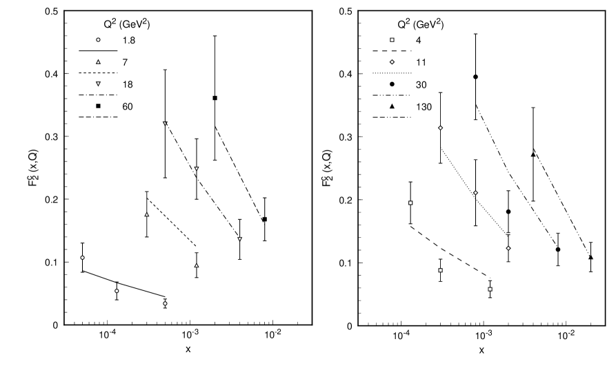
Figure 6: Order $\alpha_{s}$ 4-flavor general mass calculation compared to the recent ZEUS data on $F_{2}^{c}$. The calculation uses the CTEQ5HQ parton distributions with $m_{c}=1.3GeV$.

4 Semi-inclusive Cross Sections with Tagged Charm Hadrons

4.1 General considerations

Now we consider semi-inclusive cross sections, with a charm hadron tagged in the final state. Naively, to compute this cross section, one simply convolves the cross sections for parton final states, Eqs. 11 and 12, with a suitable fragmentation function of partons into the final charm hadron. However, the factorization of the final state particles through fragmentation functions is only rigorously defined in the limit $Q^{2}\gg m_{c}^{2}$. Thus, the treatment of tagged charm particles in the final state can only be systematically applied at high energies, using the 4-flavor scheme. However, it is a common practice to introduce fragmentation functions into charm hadrons even in the 3-flavor scheme, and for energies not far above threshold. This approach should be considered a convenient phenomenological model of hadronization, perhaps adequate for current experimental accuracy, rather than rigorous theory. We follow this practice in our calculation, employing fragmentation functions over the full range of $Q^{2}$, while maintaining the correct factorization-scheme implementation at high $Q^{2}$.

The fragmentation functions $d_{a}^{H}(x,\mu)$ obey the standard (mass-independent) QCD evolution equations, and are determined from suitable initial functions at some given scale $\mu=Q_{0}$, of the order of $m_{c}$. Following Mele and Nason [29], for a given final-state charm hadron ${H},$ we write

$$d_{a}^{H}(x,Q_{0})=d_{a}^{c}(x,Q_{0})\otimes D_{c}^{H}(x,Q_{0})$$ (13)

where the partonic charm fragmentation functions $\left\{d_{a}^{c};a=l,c\right\}$ are perturbatively calculable, and $D_{c}^{H}(x,Q_{0})$ is considered non-perturbative and is to be obtained by comparison with experiment.

For the perturbatively calculable fragmentation functions, Ref. [29] gives, to order $\alpha_{s}$:

$$d_{c}^{c}(x,Q_{0}) = \delta(1-x)+{\frac{{\alpha_{s}(Q_{0})C_{F}}}{{2\pi}}}\left[{\frac{{1+x^{2}}}{{1-x}}}\left(\ln{\frac{{Q_{0}^{2}}}{{m_{c}^{2}}}}-2\ln(1-x)-1\right)\right]_{+}$$

$$d_{g}^{c}(x,Q_{0}) = {\frac{{\alpha_{s}(Q_{0})T_{F}}}{{2\pi}}}(x^{2}+(1-x)^{2})\ln{\frac{{Q_{0}^{2}}}{{m_{c}^{2}}}}$$ (14)

$$d_{q,\bar{q},\bar{c}}^{c}(x,Q_{0}) = 0$$

where $T_{F}=1/2$ and $C_{F}=4/3$.  In keeping with the choice of the matching scale in our overall calculation, we choose $Q_{0}=m_{c}$ for convenience in this paper.

For the non-perturbative charm quark into charmed mesons fragmentation function $D_{c}^{H}(z),$ we used the conventional Peterson form [30],

$$D_{c}^{H}(z)=\frac{A}{z[1-1/z-\epsilon/(1-z)]^{2}},$$ (15)

For the charm meson $D^{(\ast)},$ which will be our focus because of available experimental data, we take $\epsilon=0.02,$ cf. [31], and a value for $A$ such that the branching fraction $B(c\rightarrow D^{\ast})=0.22$ [32]. We note that, although the perturbative fragmentation functions, Eq. 14, contain singular (generalized) functions, the overall parton-to-charm-meson fragmentation functions $d_{a}^{H}(x,\mu),$ Eq. 13, are well behaved after convolution with the above non-perturbative fragmentation function $D_{c}^{D^{(\ast)}}(z)$.

In principle, after evolving to high enough $Q^{2}$ so that $\alpha_{s}\log(Q^{2}/m_{c}^{2})$ is of order one, all of the fragmentation functions $d_{c}^{H},\ d_{g}^{H},\ d_{q,\bar{q},\bar{c}}^{H}$ eventually become of the same size.  In practice, however, at HERA energies we find $d_{c}^{H}\gg d_{g}^{H}\gg d_{q,\bar{q},\bar{c}}^{H}$. For currently required accuracy, it suffices to keep only the charm-to-hadron contributions, proportional to $d_{c}^{H}$. In this approximation, our calculation of the cross section with a tagged charm hadron can be written in the 4-flavor scheme as

$$\begin{array}[]{lll}F_{A,\lambda}^{H}(Q^{2},x,..)&=&\;\;f_{A}^{g}\otimes\,^{1}\omega_{g,\lambda}^{c\bar{c}}\otimes\,d_{c}^{H}\\ &&+\,(f_{A}^{c}-\;f_{A}^{g}\otimes\,^{1}\tilde{f}_{g}^{c}-f_{A}^{c}\otimes\,^{1}\tilde{f}_{c}^{c})\,\otimes\,^{0}\omega_{c,\lambda}^{c}\otimes\,d_{c}^{H}\\ &&+\;f_{A}^{c}\otimes\,^{1}\omega_{c,\lambda}^{cX}\otimes\,d_{c}^{H}\ .\end{array}$$ (16)

To ensure that this calculation is adequate, we have also calculated the contribution from one of the more important remaining subprocesses: gluon fragmentation in an order $\alpha_{s}$ light parton hard scattering, i.e. $\gamma^{\ast}q\rightarrow gq\ ;\ g\rightarrow H$. It is given by: $f_{A}^{q}\otimes\,^{1}\widehat{\omega}_{q,\lambda}^{qg}\otimes\,d_{g}^{H}$, where $d_{g}^{H}$ is the gluon fragmentation function computed from Eqs. 13 and 14. We have verified that its contribution remains small throughout the current energy range. It becomes more noticeable only in the large $Q$ limit. However, in this limit, the gluon fragmentation function term is not infra-red safe by itself. To insure consistency at high energies, one needs to include a full set of infra-red safe higher order subprocesses along with it. The full calculation is more appropriately considered as part of the next order project.

At the same level of accuracy, it is also reasonable to ignore the evolution of $d_{a}^{H}(x,\mu(x,Q))$, since the effect of QCD evolution is not significant over the currently accessible HERA $Q$ range. One can use the un-evolved $d_{c}^{H}(x,\mu=Q_{0})$ in place of the fully evolved $d_{c}^{H}(x,\mu(x,Q,m_{c}))$ with much gain in efficiency of calculation and little sacrifice in accuracy. The error incurred is of the same order as that incurred by neglecting the subleading fragmentation functions, $d_{g}^{H}$ and $d_{q,\bar{q},\bar{c}}^{H}$ ; and the comments on accounting for $\ln(m_{c})$ factors made there also apply here. To be sure about this, we have performed the calculation both with and without evolving $d_{c}^{H}.$ The difference is indeed small. Therefore, in all our subsequent plots we shall include only the direct charm-to-hadron contributions of Eq. (16) with the un-evolved fragmentation function $d_{c}^{H}(x,Q_{0})$.

4.2 Differential distributions

We employ the Monte Carlo method to carry out the numerical phase-space integration; the new program package is implemented in the C++ programming language. Therefore, we can generate differential distributions involving final-state charm mesons, incorporating kinematic cuts appropriate for specific experimental measurements, in addition to fully inclusive cross-sections.

In working with on-mass-shell heavy flavor quarks and hadrons in the parton language, there is an ambiguity in defining the momentum fraction variables $x\;(z)$ for the parton distribution (fragmentation) function.  This problem arises in all schemes; and it goes away at high energies ($Q\gg m_{c}$), where the parton picture becomes accurate. Following the modern practice in proofs of factorization, we define the momentum fraction variables as ratios of the relevant light-cone momentum components, e.g.$\;p_{D}^{+}=zp_{c}^{+}$ for fragmentation of a charm quark into a $D$ meson. Other authors, e.g. [8, 34], use the prescription $\vec{p}_{D}=z\vec{p}_{c}$ and adjust the energy variable to enforce the mass-shell condition. At moderate energies, any noticeable differences in results due to the choice of this prescription signals that the calculation using fragmentation functions is outside the region of applicability of the parton formalism. We have verified that the results presented below are insensitive to the choice between the two prescriptions.

The QCD formula, Eq. 16, contains three scale choices in principle: the renormalization scale, the factorization scale and the fragmentation scale. For simplicity, we choose the same energy scale $\mu(x,Q,m_{c})$ for all three. As in the case of the inclusive $F_{2}^{c}(x,Q)$, for results shown below, we choose the simple function $\mu=c(Q^{2}+m_{c}^{2})^{1/2}$, which characterizes the typical virtuality of the process. The constant $c$ is of order 1; and is varied over same range when we try to estimate the scale-dependence of the physical predictions. The magnitude of the charm cross-section is sensitive to the value of $m_{c}$. For results presented here, we use $m_{c}^{\overline{\rm MS}}=1.3GeV$, the value used in the CTEQ5HQ parton distribution analysis (which is in the middle of the range given by the PDG review).

Fig. 7 shows plots of four differential distributions for $D^{\ast}$ production at HERA, calculated using the NLO ($\alpha_{s}$) generalized $\overline{{\rm MS}}$ 4-flavor formalism described above.  The kinematic variables and their ranges correspond to those of the 1996-97 ZEUS data: $1<Q^{2}<600\;$GeV${}^{2}\;;\;0.02<y<0.7\;;\;1.5<p_{T}^{D^{\ast}}<15\;$GeV ; $\left|\eta_{D^{\ast}}\right|<1.5.$ Each distribution contains two curves obtained with two values of the constant $c=0.5,1$ in the definition of the scale parameter described above. These predictions, using the CTEQ5HQ parton distributions, are compared to the ZEUS data [28]. We observe a rather large scale dependence in these results. This is not surprising, since the compensation among the various subprocesses which underlie the scale-independence of the physics predictions (up to some order of perturbation theory), strictly speaking, only apply to the inclusive cross-section. The experimental kinematical cuts implemented in these exclusive calculations to some extent undermine the mutual cancellation between diagrams which are necessary for relatively scale-independent predictions. For example, the order $\alpha_{s}^{0}$ $\gamma^{*}c\rightarrow c$ HE term (which resums the logarithms arising from the near-collinear configurations of an infinite tower of higher-order diagrams) implements the full contribution in collinear kinematics, a clear over-simplification.

Keeping this fact in mind, and with current relatively large experimental errors, the results of Fig. 7 can be considered rather encouraging: the $Q^{2}$ and $p_{T}$ distributions show very good general agreement; while the $W$ and $\eta_{D}$ distributions are “in the right ball park”, the shapes are too scale-dependent to allow for meaningful “predictions”. (A specific choice of scale, in between the two shown, will actually yield theory curves in reasonable agreement with data, within errors.) In order to make genuine predictions on differential distributions in the 4-flavor scheme, it is necessary to extend the calculation to order $\alpha_{s}^{2}$, which would be NNLO in the 4-flavor scheme. This can be done by transforming already available NLO results for 3-flavor calculations into the 4-flavor scheme. At the same order in $\alpha_{s}$, the 4-flavor scheme calculation is, of course, more involved than the (NLO) 3-flavor one because of the need for including the necessary subtraction terms in a NNLO calculation – such as those appearing in Eqs. 7, 9, and 11.

The calculation of these differential distributions in the $\alpha_{s}^{2}$ 3-flavor FFN scheme was carried out by [34]. Generally good agreement between these calculations and the recent ZEUS data, using specific parton distributions, scale choices, etc. has been reported in Ref. [28]. Although the dependence of the predictions to the scale choice was not discussed in this comparison, it is relatively mild, according to [34]. This is to be expected, because the sensitivity to cuts is reduced with a better approximation of the final state particle configurations provided by the order $\alpha_{s}^{2}$ calculation. This fact implies greater predictive power for the differential distributions than the order $\alpha_{s}$ 4-flavor calculation.

The $\eta_{D^{\ast}}$ distribution in both the 3-flavor and the 4-flavor calculations appear to differ in shape compared to the existing data points. This could be due to the inadequacy of applying the fragmentation function approach at less than asymptotic region, as discussed in the beginning of this section. In particular, if the $D^{\ast}$ is not collinear to the parton, as assumed in this approach, the rapidity distribution will be affected. More extensive study of this effect is obviously needed.

Figure 7: Four differential distributions for $D^{\ast}$ production at HERA, calculated using the NLO $\left(\alpha_{s}\right)$ generalized $\overline{{\rm MS}}$ 4-flavor formalism and $m_{c}=1.3GeV$. The two curves on each plot results from two choices of the scale constant $c=0.5,1$. The data points are results from the ZEUS 96-97 run [28].

5 Conclusions

In this work we have shown how the generalized $\overline{{\rm MS}}$ formalism can be used to calculate the production of a heavy quark over a wide range of energies, from threshold to high $Q^{2}$. For charm production, the formalism consists of a 3-flavor scheme calculation at low energies, a 4-flavor scheme calculation at high energies, a matching condition between the two schemes, and a transition scale chosen at which one switches between the two schemes. Specifically, we have extended the original ACOT calculation for charm production at HERA by adding those terms which are necessary to bring the 4-flavor part of the calculation to NLO accuracy at high energies. This brings our calculation to the same level of accuracy as the other theoretical inputs to the CTEQ and MRS global QCD analyses.

The generalized $\overline{{\rm MS}}$ formalism is ideally suited for inclusive calculations, such as $F_{2}(x,Q)$ in DIS. We have shown that for a physically-motivated choice of the renormalization/factorization scale, $\mu$, the transition scale can be chosen rather low, so that our 4-flavor scheme can be used in the HERA energy range with excellent agreement compared to data, and with considerable economy compared to the more elaborate NLO 3-flavor calculation. The calculation is much simpler and the resulting program runs faster. Furthermore, the NLO corrections are much smaller in the 4-flavor calculation. This suggests that the resummation involved in the charm quark distribution function picks up the most important higher-order corrections even at modest energies. It also indicates that the perturbation series in the 4-flavor calculation is very well-behaved.

Our calculation has been implemented as a Monte Carlo program, so that we have also calculated differential distributions for exclusive charm final states. By incorporating experimental cuts in the Monte Carlo we are able to ensure that our calculation is compared directly with the data, without the need for any theoretical extrapolation to all of phase space. The agreement with HERA data is reasonable. However, in this case the 3-flavor NLO calculation has somewhat of an edge, because there is no approximation on the kinematics as is necessary in the resummation used in the 4-flavor calculation.

The comparison between available data and the order $\alpha_{s}$ 4-flavor and order $\alpha_{s}^{2}$ 3-flavor calculations discussed in the last two sections demonstrates the complementary nature of the two schemes – both with regard to the kinematic regions and to the physical quantities they are suitable for.  With more abundant and more precise experimental data on charm production, the composite generalized $\overline{{\rm MS}}$ formalism, which encompasses both, will be needed to make reliable comparisons. With this in mind we are now ready to extend the 4-flavor calculation to include the necessary ${\cal O}(\alpha_{s}^{2})$ terms, along with the ${\cal O}(\alpha_{s}^{2})$ matching conditions. Such a calculation would include all the advantages the current calculation has in addition to the advantages of the current 3-flavor NLO calculation.

Finally, the generalized $\overline{{\rm MS}}$ formalism provides a framework to extract information on the gluon and the charm distributions of the nucleon – to the same accuracy as the overall NLO global QCD analysis based on total DIS structure functions and other hard processes. Having established that our calculation does a reasonable job in describing the existing HERA data, we are now in a position to explore the question of whether the proton contains a non-perturbative charm component [35]. Certainly, it must at some level, so the real question is how small is it? The handle on the charm distribution is unique to the generalized formalism, since the fixed 3-flavor scheme does not allow the charm parton as an independent degree of freedom. We note that there have been recent phenomenological studies of “intrinsic charm” which take the theoretical cross-section to be the simple sum of the 3-flavor FFN scheme formulas and an intrinsic charm contribution by the heavy-quark excitation mechanism [36, 37, 38]. This approach cannot be internally consistent, because the 3-flavor calculation assumes parton evolution with no charm quark distribution, while “intrinsic charm” explicitly requires one. The intimate interplay between the hard matrix elements and parton evolution is consistently incorporated only in the generalized $\overline{{\rm MS}}$ scheme. Although there has been a recent effort to examine this problem incorporating some of the ideas of the general scheme [39], a fully consistent study, preferably based on more extensive data, still awaits to be done.

Acknowledgments

We would like to thank Brian Harris for many helpful discussions and especially for providing us with the code for the NLO 3-flavor calculations, and for verification of the numerical results. We would also like to thank John Collins and Fredrick Olness for many discussions and help; Jim Whitmore for assistance about the ZEUS data; and Jack Smith for discussions on the extensive order $\alpha_{s}^{2}$ calculations carried out by the Stony-Brook/Leiden group and for clarification of the proper references to their work. This work was supported in part by the US National Science Foundation under grants PHY9802564 and PHY9722144.

Appendix A Formalism for Inclusive DIS Cross Section

In this appendix, we give a concise and careful presentation of the general formalism, including the relatively simple operational procedure for calculating its various components. We hope this will help fill the gap between the original, relatively sketchy, ACOT paper [12] and the recent, more technical, all-order proof of the formalism by Collins [13].

The basis for all discussions is the factorization theorem in the presence of non-zero quark masses [13], Eq. 4. To establish this theorem in PQCD (cf. Eq. 17 below), and to give precise meaning to the various factors, one must work with partonic cross-sections and parton distributions inside partons, rather than the corresponding physical quantities which appear in Eq. 4. In this concise summary, we proceed as follows: (i) spell out the operational procedure to establish the factorization formula and calculate the hard cross-sections in any scheme; (ii) describe the specifics of the 3-flavor and 4-flavor schemes respectively; (iii) discuss the matching conditions between the two; and (iv) consider the transition from one to the other in the composite scheme, which constitutes the general formalism of Collins [13]. We finish with some remarks on the meaning of “LO” and “NLO” calculations in different schemes.

A.1 Procedure to define the factorization scheme and calculate the hard cross-sections

Given the QCD Lagrangian, with non-zero masses for the heavy quarks, one arrives at the general factorization formula for partonic cross-sections and parton distributions as follows:

• (i) Start with a set of relevant partonic structure functions $\omega_{a}$ similar to the left-hand side of Eq. (4) but with on-shell parton targets and calculate them in perturbation theory in a given renormalization scheme (i.e. with specific ultra-violet counter-terms) to a given order in $\alpha_{s}$. The result $\omega_{a}(\frac{Q}{\mu},x,\frac{m_{c}}{\mu},\frac{1}{\epsilon},\alpha_{s}\left(\mu\right))$ will depend on the renormalization scale $\mu$ and will contain collinear singularities (represented by $\frac{1}{\epsilon}$) as well as potentially large logarithm terms of the form $(\alpha_{s}\ln(\frac{\mu}{m_{c}}))^{n}$. (For simplicity we do not differentiate between the renormalization scale $\mu_{R}$ and the factorization scale $\mu_{f},$ both of which are taken in practice to be of order $Q$.)

• (ii) Independently, calculate the set of process-independent perturbative partonic distribution functions $\tilde{f}_{a}^{b}$ in the same renormalization scheme, using either the (moment-space) operator-product expansion or, equivalently, the ($x$-space) bi-local operator definition of the distribution functions. Both ultra-violet and collinear singularities appear in this calculation. The ultra-violet singularities are removed by additional counter-terms which, along with the coupling constant renormalization counter-terms, define the factorization scheme. The result takes the form $\tilde{f}_{a}^{b}(x,\frac{m_{c}}{\mu},\frac{1}{\epsilon},\alpha_{s}\left(\mu\right))$.

• (iii) Confirm that all collinear singularities in the form of $\frac{1}{\epsilon}$ terms, appearing in $\omega_{a}(\frac{Q}{\mu},x,\frac{m_{c}}{\mu},\frac{1}{\epsilon},\alpha_{s}\left(\mu\right))$ appear in the universal form given in the process-independent functions $\tilde{f}_{a}^{b}(x,\frac{m_{c}}{\mu},\frac{1}{\epsilon},\alpha_{s}\left(\mu\right))$, so that they can be factorized out in the manner of Eq. (4),

  $$\omega_{a}(\frac{Q}{\mu},x,\frac{m_{c}}{\mu},\frac{1}{\epsilon},\alpha_{s}\left(\mu\right))=\mathrel{\mathop{\sum}\limits_{b}}\tilde{f}_{a}^{b}(x,\frac{m_{c}}{\mu},\frac{1}{\epsilon},\alpha_{s}\left(\mu\right))\otimes\widehat{\omega}_{b}(\frac{Q}{\mu},x,\frac{m_{c}}{\mu},\alpha_{s}\left(\mu\right))\;,$$ (17)

  with $\widehat{\omega}_{a}$ being fully infra-red safe in the sense that it is free of all $\frac{1}{\epsilon}$ dependence. In the 4-flavor scheme defined below, the functions $\tilde{f}_{a}^{b}(x,\frac{m_{c}}{\mu},\frac{1}{\epsilon},\alpha_{s}\left(\mu\right))$ will also contain the same large logarithmic terms as $\omega_{a}(\frac{Q}{\mu},x,\frac{m_{c}}{\mu},\frac{1}{\epsilon},\alpha_{s}\left(\mu\right))$, so that these too factorize in Eq. (17) with the result that $\widehat{\omega}_{a}$ is free of all $(\alpha_{s}\ln(\frac{\mu}{m_{c}}))^{n}$ terms, and it is well-behaved as $m_{c}\rightarrow 0.$

• (iv) Systematically invert Eq. (17) to solve for the set of finite hard cross-sections $\widehat{\omega}_{a},$ which are then used in Eq. (4) for calculating physical structure functions.

There are two points to note: (a) The inversion of Eq. (17) order-by-order in the perturbation series is equivalent to subtracting the singularities contained in $\tilde{f}_{a}^{b}$ from $\omega_{a};$ (b) There is no need to set the quark mass(es) to zero anywhere in the above procedure.

In the following, we apply the above procedure to define the two simple renormalization schemes, involving 3 or 4 active quark flavors, which underlies the general approach of Refs. [9, 13]; and combine them to define the latter in the subsection under the heading of the generalized $\overline{{\rm MS}}$ formalism. These discussions are applicable to all orders in perturbation theory. Throughout these discussions, the three quarks $\left\{u,d,s\right\},$ with masses comparable to or less than $\Lambda,$ will be referred to as light quarks, and denoted collectively by $q$. The collection of light quarks plus the gluon $g$ will be referred to as light partons, and denoted by $l$. As mentioned earlier, although the formalism applies to all heavy quarks $\left\{c,b,t\right\},$ we shall use the case of charm as a generic representative, for concreteness and clarity – hence the 3- and 4-flavors.  Because the real charm quark mass $m_{c}$ is not large compared to the on-set of the region of applicability of PQCD, the 4-flavor scheme plays a more prominent role in practical applications discussed in the main body of this paper. For a heavier quark, the two corresponding schemes and their proper matching, as discussed in the rest of this (theoretical) section, will be more relevant.

A.2 Three-flavor Scheme

The 3-flavor scheme is precisely defined by choosing to work with only 3 active quark flavors, consisting of the light quarks, and using the subtraction procedure of Ref. [19]. The prescription for subtracting ultra-violet divergences encountered in the calculation of the partonic structure functions depends on the particle that produces the divergence. Broadly speaking, divergences due to the light partons $l,$ are removed using $\overline{\mbox{MS}}$ counter terms, whereas those due to the charm quark $c$ are removed by BPH zero-momentum subtraction counter terms. The precise definition can be found in Ref. [13]. This ultra-violet subtraction scheme has the nice feature that the charm quark explicitly decouples as its mass becomes large. In particular, the operators which make up the charm quark distribution function are suppressed by powers of order $\Lambda^{2}/m_{c}^{2}$. Since these terms are power-suppressed in the “heavy quark” mass, they are usually excluded from the 3-flavor scheme parton picture.

In practice then the partonic calculations in this scheme are done by considering diagrams where the massive charm quark can only appear in the final state, and there are no charm quark distribution functions, cf. Fig. 3. The light parton distributions always evolve according to the 3-flavor DGLAP equation, for all values of the renormalization scale $\mu$—both below and above the heavy quark production threshold. The parton distribution functions defined in this scheme will be restricted to the light parton $l=\left\{g,q,\bar{q}\right\}$ sector, and they will be denoted by ${}^{3}f_{A}^{l}$. In the perturbative calculation, ${}^{3}\tilde{f}_{l}^{l^{\prime}}$ contains $\epsilon^{-1}$ pole terms which are due to collinear singularities. The lowest order (LO, $\mathcal{O}(\alpha_{s}^{1})$) partonic process in which the charm quark appears in this scheme is the $\gamma^{\ast}g\rightarrow c\bar{c}$ “heavy-flavor creation” (HC) process (also known as boson-gluon fusion), corresponding to the diagrams of Fig.(3a). The associated partonic structure function, denoted by $\omega_{g}^{c\bar{c}},$ is finite. The next-to-leading order (NLO) contribution includes the 1-loop virtual corrections to $\gamma^{\ast}g\rightarrow c\bar{c}$ (cf. Fig.(3b)), plus the real partonic HC processes $\gamma^{\ast}l\rightarrow c\bar{c}l$ (cf. Fig.(3c)). The collinear divergences which appear in the calculation of the $\mathcal{O}(\alpha_{s}^{2})$ partonic structure functions ${}^{3}\omega_{g}^{c\bar{c}}$ and ${}^{3}\omega_{l}^{c\bar{c}l}$ arise from splitting of massless light partons in the collinear configuration, and take the form of $\epsilon^{-1}$ pole terms, precisely corresponding to those appearing in ${}^{3}\tilde{f}_{l}^{l^{\prime}}$ mentioned above. That is, the partonic structure functions have the factorized structure shown in Eq. (4), and the hard cross-section functions $\hat{\omega}_{l}$ will be free from $\epsilon^{-1}$ collinear singularities. This 3-flavor scheme is the one used by Ref. [7] to calculate charm production to NLO, i.e. $\mathcal{O}(\alpha_{s}^{2})$.

At high energies the hard cross-sections calculated in this scheme contain powers of $\ln(Q^{2}/m_{c}^{2}),$ as mentioned in the introduction. The perturbative expansion should be accurate at energy scales not too far above threshold, or $Q^{2}\sim m_{c}^{2},$ where $\ln(Q^{2}/m_{c}^{2})$ is of order $1$. However, at high $Q^{2}\gg m_{c}$ the perturbative expansion parameter is effectively $\alpha_{s}\ln(Q^{2}/m_{c}^{2}),$ and the large logarithm factor spoils the convergence of the perturbative series. In other words, the “hard cross-sections” $\hat{\omega}_{a}$ defined in this scheme are finite, but not infra-red safe in the limit $\frac{m_{c}}{Q}\rightarrow 0$.

A.3 Four-flavor scheme with non-zero $m_{c}$

In order to better deal with these logarithms at high energies it is more useful to use the 4-flavor scheme, in which the renormalization of $\omega_{a}$ and $\tilde{f}_{a}^{b}$ is carried out using dimensional regularization and the $\overline{\mbox{MS}}$ counter terms for all Feynman diagrams, while keeping the full quark mass dependence ($m_{c}$) of the Lagrangian.

Charm distribution functions calculated in this scheme, ${}^{4}\tilde{f}_{a}^{c}$ ($a=l,c$), are not suppressed as in the 3-flavor scheme, but contain powers of $\ln(m_{c}/\mu)$, along with possible $\epsilon^{-1}$ poles. Because of the different subtraction procedures used in the two schemes, even the light parton distributions ${}^{4}\tilde{f}_{l}^{l^{\prime}}$ will differ from ${}^{3}\tilde{f}_{l}^{l^{\prime}}$ by a finite renormalization in general. (We will return to this point later.) Because renormalization constants in the $\overline{\mbox{MS}}$ subtraction procedure are independent of mass, the evolution kernels for the ${}^{4}\tilde{f}_{a}^{b}$ parton distributions will be the same as the corresponding ones in the familiar zero-mass 4-flavor case. This is a significant convenience. The perturbative parton distribution functions ${}^{4}\tilde{f}_{a}^{b}$ have been calculated to NLO in Ref. [40].

Since charm also has a parton interpretation in this scheme, the set of partonic processes are expanded to include those involving charm initial states. The LO partonic process that involves the charm quark in the 4-flavor scheme is the $\gamma^{\ast}c\rightarrow c$ “heavy-quark excitation” (HE) process (Fig.(4a)). NLO charm quark contributions in the 4-flavor scheme come from the 1-loop virtual corrections to HE $\gamma^{\ast}c\rightarrow c$ (Fig.(4b)), and from the real HE $\gamma^{\ast}c\rightarrow gc$ and HC $\gamma^{\ast}g\rightarrow c\bar{c}$ processes (Fig.(4c,d)). Partonic structure functions $\omega_{a}$ calculated beyond LO in this subtraction scheme contain both $\epsilon^{-1}$ poles (due to collinear singularities associated with light degrees of freedom) and powers of mass-logarithms, $\ln(Q/m_{c})$, (due to collinear configurations associated with the heavy degree of freedom), just as in the 3-flavor scheme. The important difference compared to the latter case is that these potentially large logarithm terms also appear in the 4-flavor parton distributions ${}^{4}\tilde{f}_{a}^{b}$. Consequently, they are systematically factored out from $\omega_{a}$ when we obtain the hard cross-sections $\hat{\omega}_{a}$ by inverting the factorization formula Eq. (17). The charm distribution function represents the resummed contribution of all the large (infra-red unsafe) logarithm terms in $\omega_{a}.$ As a result, $\hat{\omega}_{a}$ is free from both types of collinear “singularities” (in quotes since the logarithms become singular only in the zero-mass limit). In effect, all logarithm factors $\ln(Q/m_{c})$ in $\omega_{a}$ are replaced by $\ln(Q/\mu)$ in $\hat{\omega}_{a}$, (with accompanying finite subtractions), and the latter is infra-red safe in the $\frac{m_{c}}{Q}\rightarrow 0$ limit. Thus, the 4-flavor scheme has a well-defined high energy limit, and is expected to give a much more reliable description of the physics of charm production at large $Q$ than the 3-flavor scheme.

As formulated above, the hard cross-sections still contain finite charm-mass dependence, i.e. $\hat{\omega}_{a}=\hat{\omega}_{a}(x,\frac{Q}{\mu},\frac{m_{c}}{Q},\mu)$. Being infra-red safe, as $m_{c}/Q\rightarrow 0,$ the limit $\hat{\omega}_{a}(x,\frac{Q}{\mu},\frac{m_{c}}{Q},\mu){\rightarrow}\hat{\omega}_{a}^{m_{c}=0}(x,\frac{Q}{\mu},\mu)$ is well defined. In this limit, the 4-flavor scheme with non-zero charm mass reduces to the conventional zero-mass (ZM) 4-flavor parton scheme, as mentioned in the introduction. As emphasized in Ref. [12], however, the factorization of potentially dangerous $\ln(m_{c})$ terms does not require taking the $m_{c}\rightarrow 0$ limit in the infra-red safe coefficient functions. The conventional practice of always setting $m=0$ in the hard cross-section $\hat{\omega}_{a}(x,Q,\mu)$ is a convenience, not a necessity; it results from the use of dimensional regularization of the zero-mass theory as a simple and efficient way to classify and to remove the collinear singularities. For a “heavy quark” with non-zero mass $m_{c},$ this convenient method of achieving infra-red safety is not a natural one (as it is for light flavors), since $m_{c}$ itself already provides a natural cutoff. In other words, the theory has no real collinear “singularities” associated with the charm quark, and the universal (i.e. process-independent) and potentially large mass-logarithms can be factorized systematically as outlined above. In fact, by keeping the charm quark mass dependence, this scheme can be extended down to lower values of $Q$ with much more reliable results than in the zero-mass case. This is possible because of the well-defined relation between the 4-flavor calculation with non-zero $m_{c}$ and the 3-flavor (FFN) calculation; e.g. at order $\alpha_{s}$, Ref. [12] showed that, for given $x,Q$

$${}^{4}F_{2}^{c}(x,\frac{Q}{\mu},\frac{m_{c}}{\mu})\,\mathrel{\mathop{\longrightarrow}\limits_{\lim\,\mu\rightarrow m_{c}}}\,{}^{3}F_{2}^{c}(x,\frac{Q}{\mu},\frac{m_{c}}{\mu})\rule{40.00006pt}{0.0pt}{\cal{O}}(\alpha_{s})$$ (18)

where the superscripts 3,4 refer to the 3- and 4-flavor scheme calculations respectively. To distinguish this more general 4-flavor scheme from the conventional zero-mass (ZM) 4-flavor scheme, we can refer it as the general-mass (GM) 4-flavor scheme.

The theoretical result (Eq. 18) does not, however, constrain the threshold behavior of the predicted physical structure function in the limit of $\lim\thinspace Q\,\,({\rm or}\,W)\rightarrow m_{c}$; to make a physical prediction, one needs to first choose $\mu$ as a function of the physical variables {$x,Q,m_{c}$}. This is related to the well-known scale dependence of PQCD prediction in general. We shall return to this problem at the end of the next subsection.

There is one additional advantage of the 4-flavor scheme. Since the charm quark distribution is explicitly included in the 4-flavor scheme, and since $m_{c}$ is not much larger than a typical non-perturbative scale such as the nucleon mass, one can allow for the existence of a possible nonperturbative (“intrinsic”) charm component inside a hadron at a low energy scale, say $Q_{0}$— as the boundary condition for evolution to higher scales, just like the other light flavors. This is a possibility not permitted in the 3-flavor scheme by assumption.

A.4 The generalized $\overline{{\rm MS}}$ formalism with non-zero $m_{c}$

Both the 3-flavor and the 4-flavor schemes described above are valid schemes for defining the perturbative series of the inclusive cross section in principle. They are equivalent if both are carried out to all orders in the perturbation series. At a given finite order, they differ by a finite renormalization of the distribution functions, as well as the strong coupling $\alpha_{s}$. From the physics point of view, when calculated to the appropriate order (cf. below), the 3-flavor scheme provides a more natural and accurate description of the charm production mechanism near the threshold ($Q^{2}\sim m_{c}^{2}$), whereas the 4-flavor scheme does the same in the high energy regime ($Q^{2}\gg m_{c}^{2}$), as shown in Fig. 1.

The precise definitions given in the above subsections provide the means to implement the intuitive ideas discussed in the introduction. A unified program to calculate the inclusive structure functions, including charm, which maintains uniform accuracy over the full energy range, must be a composite scheme consisting of:

• (i) the 3-flavor scheme, applied from low energy scales, of the order of $m_{c}$, and extended up;

• (ii) the 4-flavor scheme, applied from high energy scales on down; and

• (iii) a set of matching conditions which define the perturbative relation between the two schemes applied at a specific matching scale $\mu_{m}$.

It is useful to explicitly discuss all the elements of this composite scheme which link the component 3-flavor and 4-flavor calculations discussed in previous subsections to physics predictions of the general formalism:

• Choice of scale: Within each scheme ($i=3$ or $4$), one needs to specify $\mu$ as a function of the physical variables in order to make a physical prediction, i.e.

  $$F_{A,\lambda}^{phys}(Q^{2},x,m_{c})=F_{A,\lambda}^{(i)}(Q^{2},x,m_{c},\mu(x,Q,m_{c}))$$

  Although there is considerable freedom in choosing $\mu(x,Q,m_{c})$, two conditions should be met so that the prediction can be reliable: (i) $\mu$ must be of the order of $Q$ or $m_{c}$ so that PQCD applies, and (ii) $F_{A,\lambda}^{(i)}(Q^{2},x,m_{c},\mu)$ must be relatively stable with respect to variations of $\mu$ for the ($x,Q$) of interest. This is the well-known scale-dependence of any PQCD calculation. In Fig. 1, the presence of the uncertainty associated with the choice of $\mu(x,Q,m_{c})$ in each scheme is represented by the respective bands.

• Matching conditions and choice of matching scale: For a given set of arguments, $F_{A,\lambda}^{(3)}(Q^{2},x,m_{c},\mu)$ and $F_{A,\lambda}^{(4)}(Q^{2},x,m_{c},\mu)$ are not independent. Being the same physical quantity calculated in two different schemes (cf. Sec. A.2 and A.3), they are related by a finite renormalization:

  $$\begin{array}[]{c}{}^{4}\alpha_{s}(\mu)\,=\,^{3}\alpha_{s}(\mu)+\Delta\alpha\\ {}^{4}f^{a}(x,\mu)\,=\,^{3}f^{a}(x,\mu)+\Delta f^{a}(x,\mu)\end{array}\;\mbox{\rm applied at }\mu=\mu_{m}$$ (19)

  where $\Delta\alpha$ and $\Delta f^{a}(x,\mu)$ are fully calculable once the two schemes are defined. They have been calculated to order $\alpha_{s}^{2}$ [40]. Specifically, the simpler results at order $\alpha_{s}$ are [9]:

  $${}^{4}\alpha_{s}(\mu)=\,^{3}\alpha_{s}(\mu)\left[1+\frac{{}^{3}\alpha_{s}(\mu)}{6\pi}\ln\frac{\mu^{2}}{m_{c}^{2}}+\mathcal{O}(\alpha_{s}^{2})\right]$$ (20)

  $$\begin{array}[]{ccccccc}{}^{4}f^{q}(x,\mu)&=&{}^{3}f^{q}(x,\mu)&+&0&+&\mathcal{O}(\alpha_{s}^{2})\\ {}^{4}f^{g}(x,\mu)&=&{}^{3}f^{g}(x,\mu)&-&\frac{{}^{3}\alpha_{s}(\mu)}{6\pi}\ln\frac{\mu^{2}}{m_{c}^{2}}\ ^{3}f^{g}(x,\mu)&+&\mathcal{O}(\alpha_{s}^{2})\\ {}^{4}f^{c}(x,\mu)&=&0&+&\frac{{}^{3}\alpha_{s}(\mu)}{4\pi}\ln\frac{\mu^{2}}{m_{c}^{2}}\,\int\frac{dz}{z}\,(z^{2}+\left(1-z\right)^{2})\ ^{3}f^{g}(\frac{x}{z},\mu)&+&\mathcal{O}(\alpha_{s}^{2})\end{array}$$ (21)

  The scale at which these two schemes are matched will be called the matching point, and denoted by $\mu_{m}.$ Note that either scheme can still be used with $\mu$ above or below the matching point, it is just that the equations (19) are only enforced at $\mu_{m}$. In principle, $\mu_{m}$ can be chosen at any value – different choices lead to the same overall results, up to higher order corrections. As can be seen in Eqs. 20 and 21, in the generalized $\overline{{\rm MS}}$ scheme, $\Delta\alpha(\mu)$ and $\Delta f^{a}(x,\mu)$ are both of the form $\alpha_{s}(\mu)\ln(\mu/m_{c})\ C_{1}+{\cal O}(\alpha_{s}^{2})$. Thus, if one chooses $\mu_{m}=m_{c}$, both functions $\alpha(\mu)$ and $f^{a}(x,\mu)$ in the 3-flavor scheme are equal to their counterpart in the 4-flavor scheme to first order in $\alpha_{s}$ at the matching point.  Most recent works adopt this choice [9, 41, 18]; we do the same in this paper.  Although this choice is convenient, it is not required in the general formalism. The ideas behind the matching conditions, Eq. 19, are illustrated in Fig. 8 which show two possible matching points, the first being the special one $\mu_{m}=m_{c}$. This plot also shows that $\mu_{m}$ should not be chosen too far above $m_{c}$, lest the factor $\alpha_{s}\ln(\mu/m_{c})$ in the discontinuity ceases to be perturbative.

  

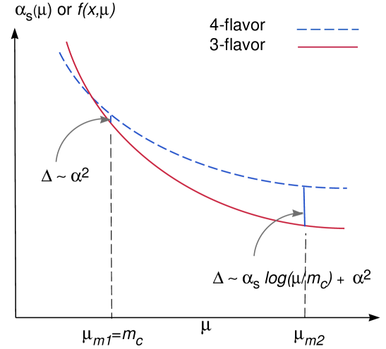
  Figure 8: Schematic illustration of the matching between 3-flavor and 4-flavor schemes. Two possible matching points are shown: the first one, $\mu_{m1}$, is at the the value $m_{c}$ where the discontinuity is of order $\alpha_{s}^{2}$; the second one, $\mu_{m2}$, is at an arbitrary value where the discontinuities are of order $\alpha_{s}ln(\mu/m_{c})$.

• Choice of transition scale: With $F_{A,\lambda}^{(i)}(Q^{2},x,m_{c},\mu(x,Q,m_{c}))$, $i=3,4$, we have two sets of calculations, one for each scheme. For physics applications, we need to specify which of these to use, say

  $$F_{A,\lambda}^{phys}(Q^{2},x,m_{c})=\{\begin{array}[]{lll}F_{A,\lambda}^{(3)}(Q^{2},x,m_{c},\mu(x,Q,m_{c}))&&Q<\mu_{t}\\ F_{A,\lambda}^{(4)}(Q^{2},x,m_{c},\mu(x,Q,m_{c}))&&Q>\mu_{t}\end{array}$$ (22)

  where we have introduced another scale $\mu_{t}$ – the transition point – where one switches from one scheme to the other, according to which one is more appropriate, as discussed in the introduction, cf. Fig.1 and the previous subsections of this appendix.

  Conceptually, the transition point is distinct from the matching point, as should be clear from their defining equations, 19 and 22. The guiding principle for choosing the optimal $\mu_{t}$ is that it should be within the region where the $F_{A,\lambda}^{(3)}$ and $F_{A,\lambda}^{(4)}$ calculations are both valid, and that their differences within this region are small. For instance, in the idealized situation depicted in Fig. 1, $\mu_{t}$ is best chosen to be in the middle of the $Q$ range where both uncertainty bands are relatively narrow.

  In practice, one can only estimate the range of uncertainties of the 3-flavor and 4-flavor calculations, say by examining the scale-dependence of the respective calculations and then make a judicious choice of $\mu_{t}$. In the case of inclusive charm production discussed in Sec. 3, Fig. 5 shows that the transition scale can be chosen at a relatively low value, close to $m_{c}$. For this choice, the composite scheme calculation reduces, in practice, to just the 4-flavor calculation.

A.5 What do “LO” and “NLO” mean?

As already mentioned in the body of this paper, in a multi-scale problem such as heavy quark production, the designation of “LO” and “NLO” to a given calculation can be rather misleading in conventional fixed-order calculations, due to the presence of large logarithms which vitiates the naive counting of powers of $\alpha_{s}$. In the composite scheme, which has a wider range of applicability than FFN schemes, the meaning of “LO” and “NLO” can be better defined, provided the relative magnitudes of the large scales are properly kept in mind. We elaborate a little bit.

• In the 3-flavor scheme, “LO” consists of the $\mathcal{O}(\alpha_{s}^{1})$ HC $\gamma^{\ast}g\rightarrow c\bar{c}$ process; whereas “NLO” involves $\mathcal{O}(\alpha_{s}^{2})$ processes such as $\gamma^{\ast}g\rightarrow gc\bar{c}$. This formal designation makes physical sense only in the threshold region.

• In the 4-flavor scheme, the “LO” process is represented by the $\mathcal{O}(\alpha_{s}^{0})$ HE $\gamma^{\ast}c\rightarrow c$ process; and the “NLO” ones consist of the $\mathcal{O}(\alpha_{s}^{1})$ HC process as well as the $\mathcal{O}(\alpha_{s}^{1})$ HE $\gamma^{\ast}c\rightarrow gc$ process. This formal designation coincides with the familiar one in the conventional treatment of DIS structure functions; it makes physical sense only when $Q^{2}\gg m_{c}^{2}$.

The apparent mismatch of orders in $\alpha_{s}$ (e.g. order $\alpha_{s}$ being “LO” in the former, but “NLO” in the latter) can be understood within the composite scheme which takes into account the order of magnitudes of the other relevant quantities in the factorization formula at the appropriate energy ranges.

Specifically, the $\mathcal{O}(\alpha_{s}^{1})$ and $\mathcal{O}(\alpha_{s}^{2})$ 3-flavor calculations lose their “LO” and “NLO” meaning as $Q^{2}$ becomes very large compared to $m_{c}^{2},$ since each power of $\alpha_{s}$ is accompanied (and neutralized) by a large logarithm $\ln(Q^{2}/m_{c}^{2})$ factor in the hard cross-section. Consequently, all terms become effectively $\mathcal{O}(\alpha_{s}^{0})$! In fact, the resummation of these large logarithms to all orders of $\alpha_{s}$ gives rise precisely to the charm distribution, resulting in the $\mathcal{O}(\alpha_{s}^{0})$ charm excitation process $\gamma^{\ast}c\rightarrow c$ of the 4-flavor scheme.  Conversely, in the 4-flavor scheme, although the charm quark distribution $f_{A}^{c}(x,Q)$ can be considered to be $\mathcal{O}(\alpha_{s}^{0})$ at high $Q^{2}$ (where all flavors are on an equal footing), as we go down to a lower energy range $Q^{2}\sim m_{c}^{2}$, one finds $f_{A}^{c}(x,Q)\sim\alpha_{s}^{1}\ln(Q^{2}/m_{c}^{2})\sim\mathcal{O}(\alpha_{s}^{1})$ compared to the dominant gluon and light quark distribution functions (assuming there is no large non-perturbative charm component). Therefore, to consistently match the 4-flavor calculation onto the LO ($\mathcal{O}(\alpha_{s}^{1})$) 3-flavor calculation, one must include both the “LO” $\mathcal{O}(\alpha_{s}^{0})$ $\gamma^{\ast}c\rightarrow c$ and the “NLO” $\mathcal{O}(\alpha_{s}^{1})$ $\gamma^{\ast}g\rightarrow c\bar{c}$ contributions, along with the associated subtraction term in the 4-flavor calculation (Cf. Ref. [12]). This implies that our 4-flavor calculation, which is NLO at high energy scales, becomes effectively “LO” near the threshold, because both the formally $\mathcal{O}(\alpha_{s}^{0})$ and $\mathcal{O}(\alpha_{s}^{1})$ contributions become of the same order of magnitude, $\mathcal{O}(\alpha_{s}^{1})$ – as in the LO 3-flavor scheme. (The calculations in the main part of this paper show that, with the natural choice of scale $\mu=\sqrt{Q^{2}+m_{c}^{2}},$ the numerical predictions of this calculation are actually fairly close to those of the NLO 3-flavor calculation, which is consistent with this observation because the size of the NLO correction is within the range of uncertainty of a LO result.)

This mixing of terms with different apparent powers of $\alpha_{s}$ is physically natural ( cf. Fig. 1 ) and logically consistent – it is a necessary feature of switching between different primary schemes, since any finite renormalization always entails a resummation (i.e. re-organization) of the perturbation series to all orders. In more concrete terms, the need for mixing terms of different apparent powers of $\alpha_{s}$ arises when:

• (i) the LO diagrams for different subprocesses start at different orders of $\alpha_{s};$

• (ii) the associated parton densities are of different numerical orders of magnitude (such as between $g,q,c$);

• (iii) the order of magnitude of a parton distribution changes as it evolves with $Q$ (such as for $c$ in the region above the threshold); and

• (iv) the hard cross-section contains logarithms of ratios of energy scales which become large.

The generalized $\overline{{\rm MS}}$ formalism, by keeping the physical $m_{c},$ provides the appropriate scheme to describe the underlying physical processes in the different regions encountered in heavy quark production.

References

- [1] H1 collaboration: C. Adloff et al., Zeit. Phys. C72 (1996) 593.
- [2] ZEUS collaboration: J. Breitweg et al., Phys. Lett. B407 (1997) 402.
- [3] E. Eichten et al., Rev. Mod. Phys. 56, 579 (1984), Erratum 58, 1065 (1986).
- [4] A. D. Martin, R. G. Roberts and W. J. Stirling, Phys. Lett. B387, 419 (1996) [hep-ph/9606345].
- [5] H. L. Lai et al., Phys. Rev. D55, 1280 (1997) [hep-ph/9606399].
- [6] P. Nason, S. Dawson, R.K. Ellis, Nucl. Phys. B327, 49 (1989), Erratum: B335, 260 (1990).
- [7] W. Beenakker, H. Kuijf, W. L. van Neerven and J. Smith, Phys. Rev. D40, 54 (1989); E. Laenen, S. Riemersma, J. Smith and W. L. van Neerven, Nucl. Phys. B392, 162 (1993); E. Laenen, S. Riemersma, J. Smith and W. L. van Neerven, Nucl. Phys. B392, 229 (1993).
- [8] S. Frixione, M. L. Mangano, P. Nason and G. Ridolfi, in Heavy Flavors II, Edited by A.J. Buras and M. Lindner. World Scientific, 1998. [hep-ph/9702287].
- [9] J. C. Collins and W. Tung, Nucl. Phys. B278, 934 (1986).
- [10] F. I. Olness and W. Tung, Nucl. Phys. B308, 813 (1988).
- [11] M. A. Aivazis, F. I. Olness and W. Tung, Phys. Rev. D50, 3085 (1994) [hep-ph/9312318].
- [12] M. A. Aivazis, J. C. Collins, F. I. Olness and W. Tung, Phys. Rev. D50, 3102 (1994) [hep-ph/9312319].
- [13] J. C. Collins, Phys. Rev. D58, 094002 (1998) [hep-ph/9806259].
- [14] W. K. Tung, in Proceedings of the 5th International Workshop on Deep Inelastic Scattering, Chicago, IL, eds. J Repond and D Krakauer, American Institute of Physics, 1997 e-Print : hep-ph/9706480.
- [15] R. S. Thorne and R. G. Roberts, Phys. Rev. D57, 6871 (1998) [hep-ph/9709442].
- [16] M. Buza, Y. Matiounine, J. Smith and W. L. van Neerven, Eur. Phys. J. C1, 301 (1998) [hep-ph/9612398]; M. Buza, Y. Matiounine, J. Smith and W. L. van Neerven, Phys. Lett. B411, 211 (1997) [hep-ph/9707263].
- [17] M. Cacciari, M. Greco and P. Nason, JHEP 9805, 007 (1998) [hep-ph/9803400].
- [18] A. Chuvakin, J. Smith and W. L. van Neerven, Phys. Rev. D61, 096004 (2000) [hep-ph/9910250].
- [19] J. Collins, F. Wilczek, and A. Zee, Phys. Rev. D 18, 242 (1978).
- [20] Cf. for instance, R. K. Ellis, H. Georgi, M. Machacek, H. D. Politzer and G. G. Ross, Nucl. Phys. B152, 285 (1979).
- [21] S. Kretzer and I. Schienbein, Phys. Rev. D58, 094035 (1998) [hep-ph/9805233].
- [22] M. Krämer, F. I. Olness and D. E. Soper, hep-ph/0003035.
- [23] J. C. Collins, A. D. Martin and M. G. Ryskin, in Proceedings of Madrid Workshop on Low X Physics, Edited by F. Barreiro, L. Labarga, J. Del Peso. Madrid, Spain, 1997,World Scientific, 1998 [hep-ph/9709440].
- [24] H. L. Lai et al. [CTEQ Collaboration], Eur. Phys. J. C12, 375 (2000) [hep-ph/9903282].
- [25] Xiaoning Wang, Heavy Quark Production in Perturbative QCD at HERA, Michigan State University Ph.D. thesis, UMI-99-22388, (1998).
- [26] E. Hoffmann and R. Moore, Z. Phys. C20, 71 (1983).
- [27] S. Riemersma, J. Smith and W. L. van Neerven, Phys. Lett. B347, 143 (1995) [hep-ph/9411431].
- [28] J. Breitweg et al. [ZEUS Collaboration], Eur. Phys. J. C12, 35 (2000) [hep-ex/9908012]; See also, B. W. Harris, hep-ph/9909310.
- [29] B. Mele and P. Nason, Nucl. Phys. B361, 626 (1991).
- [30] C. Peterson, D. Schlatter, I. Schmitt and P. Zerwas, Phys. Rev. D27, 105 (1983).
- [31] M. Cacciari, in Proceedings of Ringberg Workshop on New Trends in HERA Physic, Ringberg Castle, Tegernsee, Germany, 1997, Edited by B.A. Kniehl, G. Kramer, A. Wagner. World Scientific, 1998 [hep-ph/9708282].
- [32] K. Ackerstaff et al. [OPAL Collaboration], Eur. Phys. J. C5, 1 (1998) [hep-ex/9802008].
- [33] R. L. Jaffe and L. Randall, Nucl. Phys. B412, 79 (1994) [hep-ph/9306201].
- [34] B. W. Harris and J. Smith, Nucl. Phys. B452, 109 (1995) [hep-ph/9503484] ;Phys. Rev. D57, 2806 (1998) [hep-ph/9706334] ; and B. W. Harris, hep-ph/9909310.
- [35] S. J. Brodsky, C. Peterson and N. Sakai, Phys. Rev. D23, 2745 (1981).
- [36] B. W. Harris, J. Smith and R. Vogt, Nucl. Phys. B461, 181 (1996) [hep-ph/9508403].
- [37] J. F. Gunion and R. Vogt, hep-ph/9706252.
- [38] W. Melnitchouk and A. W. Thomas, Phys. Lett. B414, 134 (1997) [hep-ph/9707387].
- [39] F. M. Steffens, W. Melnitchouk and A. W. Thomas, Eur. Phys. J. C11, 673 (1999) [hep-ph/9903441].
- [40] M. Buza, Y. Matiounine, J. Smith, R. Migneron and W. L. van Neerven, Nucl. Phys. B472, 611 (1996) [hep-ph/9601302].
- [41] A. D. Martin, R. G. Roberts, W. J. Stirling and R. S. Thorne, Eur. Phys. J. C4, 463 (1998) [hep-ph/9803445].