Analytic coupling and Sudakov effects in exclusive processes: pion and $\gamma^{*}\gamma\to\pi^{0}$ form factors

Abstract

We develop and discuss in technical detail an infrared-finite factorization and optimized renormalization scheme for calculating exclusive processes, which enables the inclusion of transverse degrees of freedom without entailing suppression of calculated observables, like form factors. This is achieved by employing an analytic, i.e., infrared stable, running strong coupling $\alpha_{\rm s}(Q^{2})$ which removes the Landau singularity at $Q^{2}=\Lambda_{\rm QCD}^{2}$ by a minimum power-behaved correction. The ensuing contributions to the cusp anomalous dimension – related to the Sudakov form factor – and to the quark anomalous dimension – which controls evolution – lead to an enhancement at high $Q^{2}$ of the hard part of exclusive amplitudes, calculated in perturbative QCD, while simultaneously improving its scaling behavior. The phenomenological implications of this framework are analyzed by applying it to the pion’s electromagnetic form factor, including the NLO contribution to the hard-scattering amplitude, and also to the pion-photon transition at LO. For the pion wave function, an improved ansatz of the Brodsky-Huang-Lepage type is employed, which includes an effective (constituent-like) quark mass, $m_{\rm q}=0.33$ GeV. Predictions for both form factors are presented and compared to the experimental data, applying Brodsky-Lepage-Mackenzie commensurate scale setting. We find that the perturbative hart part prevails at momentum transfers above about 20 GeV ², while at lower $Q^{2}$-values the pion form factor is dominated by Feynman-type contributions. The theoretical prediction for the $\gamma^{*}\gamma\to\pi^{0}$ form factor indicates that the true pion distribution amplitude may be somewhat broader than the asymptotic one.

1 Introduction

The theoretical description of the QCD running coupling $\alpha_{\rm s}\left(Q^{2}\right)$ in the low-momentum region has attracted much interest in the last few years [1, 2, 3, 4, 5, 6, 7, 8]. In particular, the possibility of including power corrections into $\alpha_{\rm s}\left(Q^{2}\right)$, while preserving its renormalization-group (RG) invariance, enables the removal of the ghost (Landau) singularity and restores its $Q^{2}$-analyticity. Such power corrections, sub-leading in the ultraviolet (UV) region, correspond to non-analytical contributions to the $\beta$-function as to make the running coupling well-defined in the infrared (IR) regime but, being not confined within the UV regime, they are outside the operator product expansion.

The existence of power corrections in $\alpha_{\rm s}\left(Q^{2}\right)$, if true, would greatly affect our understanding of non-perturbative QCD effects. For instance, a power correction to $\alpha_{\rm s}$ gives rise to a linear term in the inter-quark static potential at short distances [9]. On a more speculative level, one may argue [7] that the source of such terms are small-size fluctuations in the non-perturbative QCD vacuum, perhaps related to magnetic monopoles in dual QCD or nonlocal condensates. Besides, and in practice, a power-behaved contribution at low scales can be used to remove the Landau singularity, present in perturbation theory, supplying in this way an IR stable, i.e., ghost-free running (effective) coupling that can be extended to the timelike region [10, 2, 3, 4, 5, 11]. As a result, re-summed expressions, which typically involve integrations down to scales $\mu\simeq\Lambda_{\rm QCD}$, are not affected by the Landau pole and can be safely evaluated.

The aim of the present work is to develop in detail a factorization and renormalization scheme, which self-consistently incorporates such a non-perturbative power correction in the running coupling, and then use it to assess and explore exclusive processes. We do not, however, propose to involve ourselves in the discussion of whether or not such power corrections have a fundamental justification within non-perturbative QCD. We consider the ambiguity in removing the Landau pole as resembling the ambiguity in adopting a particular (non-IR-finite) renormalization scheme in perturbative QCD. However, this scheme dependence will be minimized by combining our approach with the Brodsky-Lepage-Mackenzie (BLM) commensurate scale setting procedure [12]. Recall in this context that the parameter $\Lambda_{\rm QCD}$ has no special meaning in parameterizing the position of the Landau pole and can be traded for an interpolating scale $\mu$, on the basis of the renormalization-scale freedom (see, for instance, [8]). The justification for such an approach will be supplied a posteriori by the self-consistent incorporation of higher-order perturbative corrections and by removing the IR-sensitivity of perturbatively calculated hadronic observables.

A key ingredient of our approach is that the modified running coupling will be taken into account not only in the factorized short-distance part, i.e., through the fixed-order perturbation expansion, but also in the re-summed perturbative expression for the exponentiation of soft and collinear gluons (Sudakov effects) and in the RG-controlled evolution of the factorized parts. This means, in particular, that the exponent of the Sudakov suppression factor will be generalized to include power corrections, which encode long-distance physics.

To accomplish these objectives, we adopt as a concrete power-corrected running coupling an analytic model for $\alpha_{\rm s}$, recently proposed by Shirkov and Solovtsov [4], which yields an IR-finite running coupling. This model combines Lehmann analyticity with the renormalization group to remove the Landau singularity at $Q^{2}=\Lambda_{\rm QCD}^{2}$, without employing adjustable parameters, just by modifying the logarithmic behavior of $\alpha_{\rm s}$ by a (non-perturbative) minimum power correction in the UV regime.

At the present stage of evidence, it would be, however, premature to exclude other parameterizations for the behavior of the running coupling in the infrared, and one could introduce further modifications [7, 13]. It is nevertheless worth remarking that in a recent work by Geschkenbein and Ioffe [14] on the polarization operator (related to the Adler function) the same infrared limit for the effective coupling was obtained as in the Shirkov-Solovtsov approach. Furthermore, it was shown in [11] that postulating that the Adler function $D(Q^{2})$ is given by integrating $R^{\rm QCD}(s)$ over the physical region $s>0$ only, one finds a $\Lambda$-parameterization for the strong running coupling in the spacelike region which coincides with the pole-free one-loop expression proposed by Shirkov and Solovtsov [4]. Hence, the assumption of analyticity of the strong coupling in the complex $Q^{2}$ plane, used by Shirkov and Solovtsov, which at first sight might seem arbitrary, is supported by the analyticity of a physical quantity.

Whatever the particular choice of power corrections in the running coupling, it is clear, without the Landau pole, IR sensitivity of loop integrations associated with IR renormalons (see [1, 15, 16], and [17] for a recent review) is entirely absent. We emphasize, however, that the two approaches, though they both entail power-like corrections $\propto\left(\Lambda_{\rm QCD}/Q\right)^{\rm p}$, are logically uncorrelated, as the removal of the Landau pole is a strong-coupling problem (tantamount to defining a universal running coupling in the IR region), whereas IR renormalons parameterize in a process-dependent way the low-momentum sensitivity in the re-summation of large-order contributions of the perturbative series of bubble chains. In some sense the two approaches appear to have complementary scopes: employing “forced analyticity” of the running coupling attempts to incorporate non-perturbative input in terms of a power-correction term in perturbatively calculated entities, like the hard-scattering amplitude and the Sudakov suppression factor, that are in turn related to observables (e.g., form factors). The renormalon technique, on the other hand, tries to deduce as much as possible about power corrections from (re-summing) perturbation theory. Whether power corrections inferred from renormalons can link different processes (universality assumption) is an important question currently under investigation [2, 18, 19, 20, 21].

Continuing our previous exploratory study [22] (see also [23] from which the present investigation partly derives), we further extend and test our theoretical framework with build-in analyticity by including into the calculation of the pion form factor the next-to-leading order (NLO) perturbative contribution to the hard-scattering amplitude [24, 25, 26, 27]. To compute the pion form factors in the region $b\sim 1/\Lambda_{\rm QCD}$, where the hadronic size becomes important, the effects of the original ${{\bf k}_{\perp}}$ distribution of the partons inside the pion have to be included. To this end, an ansatz of the Brodsky-Huang-Lepage (BHL) type [28] for the (soft) pion wave function is adopted. This ansatz incorporates an effective (i.e., dynamically generated) quark mass to ensure that $\psi_{\pi}^{\rm soft}\left(x,{{\bf k}_{\perp}}\right)$ has the correct behavior for ${{\bf k}_{\perp}}=0$ and $k_{3}\to-\infty$. Predictions for both the pion electromagnetic and the pion-gamma transition form factor, employing a pion light-cone wave function without a mass term, were presented in Refs. [22, 23] to which we refer for further details. The influence of the mass term on the hard pion form factor is very weak and it primarily affects the soft contribution and the pion-photon transition form factor. Moreover, the specific form of the ansatz for modeling the intrinsic transverse parton momentum in the pion bound state is insignificant for the implementation of the IR-finite scheme, as its effects become relevant only for large transverse distances below $1/\Lambda_{\rm QCD}$ that are outside the scope of the present investigation.

To minimize the dependence on the renormalization scheme and scale, we obtain our results using an optimized renormalization prescription, based on the Brodsky-Lepage-Mackenzie (BLM) [12] commensurate scale setting. The effect of using a commensurate renormalization scale in calculating $F_{\pi}$ and $F_{\pi\gamma}$ is discussed quantitatively. An important observation is that the theoretical prediction for the hard (perturbative) contribution to the pion’s electromagnetic form factor exhibits no IR-sensitivity, in contrast to approaches [29, 30, 31, 27] with no IR-fixed point in the running coupling. The existence of an IR-fixed point in the effective strong coupling is implied by the general success of the dimensional counting rules.

The major virtue of such a theoretical framework, the latter being the object of this paper, is that it enables the inclusion of transverse degrees of freedom, primordial (i.e., intrinsic) [30] and those originating from (soft) gluonic radiative corrections [29, 32], without entailing suppression of perturbatively calculated observables, viz., the pion form factor, in the high-momentum region, where the use of perturbative QCD is justified, and where suppression is merely the result of an unnecessarily severe IR-regularization. This enhancement is (as noted above) due to power-term generated contributions to the anomalous dimensions of the cusped Wilson line, related to the Sudakov form factor, and such to the quark wave function that governs evolution of the factorized exclusive amplitude. These modified anomalous dimensions will be treated here to two-loop accuracy. Note that at the same time, the artificial rising trend (see, e.g., [27, 31]) of the magnitude of the hard pion form factor at intermediate and low momenta (below about 4 GeV²), which solely originates from the presence of the Landau singularity at $Q^{2}=\Lambda_{\rm QCD}^{2}$ in the effective coupling, is here entirely absent. Therefore, the scaling behavior of the perturbatively calculated pion form factor towards lower values of $Q^{2}$ resembles the one computed with a quasi constant coupling. Indeed, the scaled pion form factor is in a wide range of momenta almost a straight line, as one should expect for the leading-twist contribution (modulo logarithmic evolutional corrections which for the asymptotic distribution amplitude start at NLO and are negligible). Consequently, the magnitude of the hard part at low $Q^{2}$ is considerably reduced and falls short to account for the data. In this momentum regime the pion form factor is dominated by its soft Feynman-type contribution.

Although most of our considerations refer to the pion as a case study for the proposed IR-finite framework, the reasoning can be extended to describe three-quark systems as well. This will be reported elsewhere.

The outline of the paper is as follows. In the next section we briefly discuss the essential features of the IR-finite running coupling. In Sect. 3 we develop and present in detail our theoretical scheme. Sect. 4 extends the method to the NLO contribution to the hard-scattering amplitude. An important ingredient in the phenomenological analysis of the form factors is the BHL-type ansatz for modeling $\psi_{\pi}^{\rm soft}\left(x,{{\bf k}_{\perp}}\right)$, which includes an effective quark mass. In Sect. 5 we discuss the numerical implementation of our scheme revolving around the appropriate kinematic cuts to ensure factorization of dynamical regimes on the numerical level by appropriately defining the accessible phase space regions of transverse momenta (or equivalently transverse distances) for gluon emission in each regime. In Sect. 6 we apply these techniques to the electromagnetic and the pion-gamma transition form factor. We also provide arguments for the appropriate choice of the renormalization scale and link our renormalization prescription to BLM optimal, i.e., commensurate, scale setting. We also discuss how our scheme compares with others. Finally, in Sect. 7, we summarize our results and draw our conclusions.

2 Model for QCD running coupling

The key element of the analytic approach of Shirkov and Solovtsov [4] is that it combines a dispersion-relation approach, based on local duality, with the renormalization group to bridge the regions of small and large momenta, providing universality at low scales. The approach is an extension to QCD of a method originally formulated by Redmond for QED [33].

At the one-loop level, the Landau ghost singularity is removed by a single power correction and the IR-finite running coupling reads

$$\bar{\alpha}_{\rm s}^{{\rm an}(1)}(Q^{2}) \equiv \bar{\alpha}_{\rm s}^{{\rm pert}(1)}(Q^{2})+\bar{\alpha}_{\rm s}^{{\rm npert}(1)}(Q^{2})$$ (1)

$$= \frac{4\pi}{\beta_{0}}\left[\frac{1}{\ln\left(Q^{2}/\Lambda^{2}\right)}+\frac{\Lambda^{2}}{\Lambda^{2}-Q^{2}}\right]\;,$$ (2)

where $\Lambda\equiv\Lambda_{\rm QCD}$ is the QCD scale parameter.

This model has the following interesting properties. It provides a non-perturbative regularization at low scales and leads to a universal value of the coupling constant at zero momentum $\bar{\alpha}_{\rm s}^{(1)}(Q^{2}=0)=4\pi/\beta_{0}\simeq 1.396$ (for three flavors), defined only by group constants. No adjustable parameters are involved and no implicit “freezing”, i.e., no (color) saturation hypothesis of the coupling constant in the infrared is invoked.

Note that the IR-fixed point (i) does not depend on the scale parameter $\Lambda$ – this being a consequence of RG invariance – and (ii) extends to the two-loop order, i.e., $\bar{\alpha}_{\rm s}^{(2)}(Q^{2}=0)=\bar{\alpha}_{\rm s}^{(1)}(Q^{2}=0)\equiv\bar{\alpha}_{\rm s}(Q^{2}=0)$. (In the following the bar is dropped.) Hence, in contrast to standard perturbation theory in a minimal subtraction scheme, the IR limit of the coupling constant is stable, i.e., does not depend on higher-order corrections and is therefore universal. As a result, the running coupling also shows IR stability. This is tightly connected to the non-perturbative contribution $\propto\exp(-4\pi/\alpha\beta_{0})$, which ensures analytic behavior in the IR domain by eliminating the ghost pole at $Q^{2}=\Lambda^{2}$, and extends to higher loop orders. Besides, the stability in the UV domain is not changed relative to the conventional approach and therefore UV perturbation theory is preserved.

At very low-momentum values, say, below 1 GeV, $\Lambda_{\rm QCD}$ in this model deviates from that used in minimal subtraction schemes. However, since we are primarily interested in a region of momenta which is much larger than this scale, the role of this renormalization-scheme dependence is only marginal. In our investigation we use $\Lambda_{\rm QCD}^{{\rm an}(\rm{n_{\rm f}}=3)}=242~{}{\rm MeV}$ which corresponds to $\Lambda_{\rm QCD}^{{\overline{\rm MS}}(\rm{n_{\rm f}}=3)}=200~{}{\rm MeV}$.

The extension of the model to two-loop level is possible, though the corresponding expression is too complicated to be given explicitly [4]. An approximated formula – used in our analysis – with an inaccuracy less than $0.5\%$ in the region $2.5\,\Lambda<Q<3.5\,\Lambda$, and practically coinciding with the exact result for larger values of momenta, is provided by [4]

$$\alpha_{\rm s}^{{\rm an}(2)}(Q^{2})=\frac{4\pi}{\beta_{0}}\left[\frac{1}{\ln\frac{Q^{2}}{\Lambda^{2}}+\frac{\beta_{1}}{\beta_{0}^{2}}\,\ln\left(1+\frac{\beta_{0}^{2}}{\beta_{1}}\ln\frac{Q^{2}}{\Lambda^{2}}\right)}+\frac{1}{2}\,\frac{1}{1-\frac{Q^{2}}{\Lambda^{2}}}-\frac{\Lambda^{2}}{Q^{2}}D_{1}\right]\;,$$ (3)

where $\beta_{0}=11-\frac{2}{3}n_{\rm f}=9$, $\beta_{1}=102-\frac{38}{3}n_{\rm f}=64$, and $D_{1}=0.035$ for $n_{\rm f}=3$.

With experimental data at relatively low momentum-transfer values for most exclusive processes, reliable theoretical predictions based on perturbation theory are difficult to obtain. Both the unphysical Landau pole of $\alpha_{\rm s}$ and IR instability of the factorized short-distance part in the so-called end-point region are affecting such calculations, especially beyond leading order (LO). It is precisely for these two reasons that the Shirkov-Solovtsov analytic approach to the QCD running coupling can be profitably used for computing amplitudes describing exclusive processes [34, 35, 36], like hadronic form factors. The improvements are then: (i) First and foremost, the non-perturbatively generated power correction modifies the Sudakov form factor [32, 37, 38, 39, 40] via the cusp (eikonal) anomalous dimension [41], and changes also the evolution behavior of the soft and hard parts through the modified anomalous dimension of the quark wave function. This additional contribution to the cusp anomalous dimension is the source of the observed IR enhancement (at larger $Q^{2}$ values) of hadronic observables and helps taking into account non-perturbative corrections (power terms in $Q$ and the impact parameter $b$) in the perturbative domain, thus improving the quality and scaling behavior of the (perturbative) form-factor predictions (at low $Q^{2}$). We emphasize in this context that the ambiguity of the Landau remover is confined within the momentum regime below the factorization scale, whereas above that scale the power correction is unambiguous. Since we are only interested in the computation of the hard contribution in the region $Q^{2}\gg{{\bf k}_{\perp}}^{2}$, $Q^{2}\gg m_{\rm q}^{2}$, this ambiguity is in fact of minor importance. (ii) Factorization is ensured without invoking the additional assumption of “freezing” the coupling strength in the IR regime by introducing, for example, an (external, i.e., ad hoc) effective gluon mass in order to saturate color forces at large distances, alias, low momenta. (iii) The Sudakov form factor does not have to serve as an IR protector against $\alpha_{\rm s}$ singularities. Hence, the extra constraint of using the maximum between the longitudinal and the transverse scale as argument of $\alpha_{\rm s}$, proposed in [29] and used in subsequent works, becomes superfluous. (iv) The factorization and renormalization scheme we propose on that basis enables the optimization of the (arbitrary) constants which define the factorization and renormalization scales [32, 37, 42, 43] – especially in conjunction with the BLM commensurate-scale procedure [12]. This becomes particularly important when including higher-order perturbative corrections (see, Sect. 4).

3 Infrared-finite factorization and renormalization scheme

Application of perturbative QCD is based on factorization, i.e., how a short-distance part can be isolated from the large-distance physics related to confinement. But in order that observables calculated with perturbation theory are reliable, one must deal with basic problems, like the re-summation of “soft” logarithms, IR sensitivity, and the factorization and renormalization scheme dependence of truncated perturbative expansions.

It is one of the purposes of the present work to give a general and thorough investigation of such questions, as they are intimately connected to the behavior of the QCD (effective) coupling at low scales.

The object of our study is the electromagnetic pion’s form factor in the space-like region, which can be expressed as the overlap of the corresponding full light-cone wave functions between the initial (“in”) and final (“out”) pion states: [44, 45]

$$F_{\pi}\left(Q^{2}\right)=\sum_{n,\lambda_{i}}\sum_{q}e_{\rm q}\int\frac{[dx_{i}][d^{2}{\bf k}_{\perp i}]}{16\pi^{3}}\psi_{\pi}^{\rm out}\left(x_{i},{\bf l}_{\perp i},\lambda_{i}\right)\psi_{\pi}^{\rm in}\left(x_{i},{\bf k}_{\perp i},\lambda_{i}\right)$$ (4)

with $$[dx_{i}]\equiv\prod_{i}dx_{i}\delta\left(1-\sum_{j}x_{j}\right)$$ (6) $$[d^{2}{\bf k}_{\perp i}]\equiv\prod_{i}d^{2}{\bf k}_{\perp i}16\pi^{3}\delta^{2}\left(\sum_{j}{\bf k}_{\perp j}\right)\;,$$ (7) where the sum in Eq. (4) extends over all Fock states and helicities $\lambda_{i}$ (with $e_{\rm q}$ denoting the charge of the struck quark), and where

$${\bf l}_{\perp i}=\left\{\begin{array}[]{ll}{\bf k}_{\perp i}+(1-x_{i}){\bf q}_{\perp i}\;,&{\rm struck}\;\,{\rm quark}\\ {\bf k}_{\perp i}-x_{i}{\bf q}_{\perp i}&{\rm spectators}\;.\end{array}\right.$$ (8)

We will evaluate expression (4) using only the valence (i.e., lowest particle-number) Fock-state wave function, $\psi_{\rm q\bar{\rm q}}(x,{\bf k}_{\perp})$, which provides the leading twist-2 contribution, since higher light-cone Fock-state wave functions require the exchange of additional hard gluons and are therefore relatively suppressed by inverse powers of the momentum transfer $Q^{2}$. Furthermore, a recent study [46], based on light-cone sum rules, shows that, for the asymptotic pion distribution amplitude, the twist-4 contribution to the scaled pion form factor ($Q^{2}F_{\pi}\left(Q^{2}\right)$ is less than 0.05, whereas the twist-6 correction turns out to be negligible. As we shall see in Sect. 5, this higher-twist correction amounts to about $25\%$ of the NLO hard contribution, calculated in our scheme. This uncertainty in the theoretical prediction is much lower than the quality of the currently available experimental data.

In order to apply a hard-scattering analysis, we dissect the pion wave function into a soft and a hard part with respect to a factorization scale $\mu_{\rm F}$, separating the perturbative from the non-perturbative regime, and write (in the light-cone gauge $A^{+}=0$)

$$\psi_{\pi}\left(x,{\bf k}_{\perp}\right)=\psi_{\pi}^{\rm soft}\left(x,{\bf k}_{\perp}\right)\theta\left(\mu_{\rm F}^{2}-{\bf k}_{\perp}^{2}\right)+\psi_{\pi}^{\rm hard}\left(x,{\bf k}_{\perp}\right)\theta\left({\bf k}_{\perp}^{2}-\mu_{\rm F}^{2}\right)\;,$$ (9)

where the wave function $\psi_{\pi}(x,{\bf k}_{\perp})$ is the amplitude for finding a parton in the valence Fock state with longitudinal momentum fraction $x$ and transverse momentum ${\bf k}_{\perp}$ (we suppress henceforth helicity labels). Then the large (perturbative) $k_{\perp}$ tail can be extracted from the soft wave function via a single-gluon exchange kernel, encoded in the hard scattering amplitude $T_{\rm H}$, so that [34, 45]

$$\psi_{\pi}^{\rm hard}\left(x,{\bf k}_{\perp}\right)=\int_{0}^{1}dy\int d^{2}{\bf l}_{\perp}T_{\rm H}\left(x,{{\bf k}_{\perp}};y,{{\bf l}_{\perp}}\right)\psi_{\pi}^{\rm soft}\!\left(y,{\bf l}_{\perp}\right)\;.$$ (10)

As a result, the pion form factor in Eq. (4) can be expressed in the factorized form

$$F_{\pi}(Q^{2})= \psi_{\rm soft}^{\rm out}\otimes\psi_{\rm soft}^{\rm in}+\psi_{\rm soft}^{\rm out}\otimes\left[T_{\rm H}\otimes\psi_{\rm soft}^{\rm in}\right]+\left[\psi_{\rm soft}^{\rm out}\otimes T_{\rm H}\right]\otimes\psi_{\rm soft}^{\rm in}$$ (12)

$$+\left[\psi_{\rm soft}^{\rm out}\otimes T_{\rm H}\right]\otimes\left[T_{\rm H}\otimes\psi_{\rm soft}^{\rm in}\right]+\ldots\;,$$

where the symbol $\otimes$ denotes convolution defined by Eq. (10). The first term in this expansion is the soft contribution to the form factor (with support in the low-momentum domain) that is not computable with perturbative methods. The second term represents the leading-order hard contribution due to one-gluon exchange, whereas the last one gives the NLO correction, and the ellipsis represents still higher-order terms. We will not attempt to derive the first term from non-perturbative QCD, but we shall adopt for simplicity the phenomenological approach proposed by Kroll and coworkers in [47] (see also [30]), including, in particular, an effective (constituent-like) quark mass in the soft pion wave function for the reasons already mentioned in the introduction and based on arguments to be given below. This leads to a significantly stronger fall-off with $Q^{2}$ of the soft contribution to the space-like pion form factor, compared to their approach, whereas the hard part remains almost unaffected – as should be the case if factorization of hadronic size effects is preserved. Though Jakob and Kroll consider in [30] the option of a Gaussian $k_{\perp}$-distribution with $m_{\rm q}\neq 0$ and argue that in that case $F_{\pi}^{\rm soft}$ is significantly reduced, they do not present predictions for the form factor and do not follow this option any further (see, however, the predictions in Ref. [47]). For other, more sophisticated, attempts to model the soft contribution to $F_{\pi}(Q^{2})$, we refer to [46, 48, 49, 50].

We now employ a modified factorization prescription [29, 30], which explicitly retains transverse degrees of freedom, and define (see for illustration Fig. 1)

$$\psi_{\pi}^{\rm hard}=\psi_{\pi}^{\rm soft}\left({\bf k}_{\perp}^{2}\leq\frac{C_{3}^{2}}{b^{2}}\right)\exp\left[-S\left(\frac{C_{1}^{2}}{b^{2}}\leq{\bf k}_{\perp}^{2}\leq C_{2}^{2}\xi^{2}Q^{2}\right)\right]T_{\rm Hard}\left(Q^{2}\geq{\bf k}_{\perp}^{2}\geq\frac{C_{3}^{2}}{b^{2}}\right)\;,$$ (13)

with $b$, the variable conjugate to $k_{\perp}$, being the transverse distance (impact parameter) between the quark and the anti-quark in the pion valence Fock state. The Sudakov-type form factor $\exp(-S)$ comprises leading and next-to-leading logarithmic corrections, arising from soft and collinear gluons, and re-sums all large logarithms in the region where $\Lambda_{\rm QCD}^{2}\ll{\bf k}_{\perp}^{2}\ll Q^{2}$ [42, 43, 51]. The source of these logarithms is due to the incomplete cancellation between soft-gluon bremsstrahlung and radiative corrections. It goes without saying that the function $S$ includes anomalous-dimension contributions to match the change in the running coupling in a commensurate way with the changes of the renormalization scale (see below for more details).

Figure 1.: Illustration of the factorized pion form factor, exhibiting the different regimes of dynamics. The wiggly line denotes the off-shell photon. Gluon exchanges are not explicitly displayed. The region of hard-gluon re-scattering (LO and NLO) is contained in the short-distance part, termed $T_{\rm H}$. The blobs ${\rm e}(-S)$ represent in axial gauge Sudakov-type contributions, whereas non-perturbative effects are absorbed into the (universal) pion wave functions $\psi_{\pi}^{\rm in}$ and $\psi_{\pi}^{\rm out}$.

Going over to the transverse (or impact) configuration space (typical in eikonalization procedures), the pion form factor reads [29]

$$F_{\pi}\left(Q^{2}\right)= \int_{0}^{1}dxdy\int_{-\infty}^{\infty}\frac{d^{2}{\bf b}_{\perp}}{(4\pi)^{2}}\,{\cal P}_{\pi}^{\rm out}\left(y,b,P^{\prime};C_{1},C_{2},C_{4}\right)T_{\rm H}\left(x,y,b,Q;C_{3},C_{4}\right)$$ (15)

$$\times\;{\cal P}_{\pi}^{\rm in}\left(x,b,P;C_{1},C_{2},C_{4}\right)\;,$$

where the modified pion wave function is defined in terms of matrix elements, viz.,

$${\cal P}_{\pi}\left(x,b,P,\mu\right) = \int^{|{\bf k}_{\perp}|<\mu}d^{2}{\bf k}_{\perp}{\rm e}^{-i{\bf k}_{\perp}\cdot{\bf b}_{\perp}}{\tilde{\cal P}}_{\pi}\left(x,{\bf k}_{\perp},P\right)$$ (16)

$$= \int\frac{dz^{-}}{2\pi}{\rm e}^{-ixP^{+}z^{-}}{\left\langle 0\left|{\rm T}\left(\bar{q}(0)\gamma^{+}\gamma_{5}q\left(0,z^{-},{\bf b}_{\perp}\right)\right)\right|\pi(P)\right\rangle}_{A^{+}=0}$$ (17)

with $P^{+}=Q/\sqrt{2}=P^{-\prime}$, $Q^{2}=-(P^{\prime}-P)^{2}$, whereas the dependence on the renormalization scale $\mu$ on the rhs of Eq. (17) enters through the normalization scale of the current operator evaluated on the light cone and the dependence on the effective quark mass has not been displayed explicitly. Note that in the light-cone gauge $A^{+}=0$, the Schwinger string in Eq. (17) reduces to unity. The factorized hard part $T_{\rm H}\left(x,y,b,Q;C_{3},C_{4}\right)$ contains hard-scattering quark-gluon subprocesses, including in the gluon propagators power-suppressed corrections due to their transverse-momentum dependence. These gluonic corrections become important in the end-point region ($x\to 0$) for fixed $Q^{2}$. Furthermore, current quark masses, being much smaller than the resolution scale (set by the invariant mass of the partons) can be safely neglected in $T_{\rm H}$, so that (valence) quarks are treated on-mass shell.

A few comments on the scales involved and corresponding dynamical regimes (see Eq. (15) and Fig. 2) are in order:

• The scale $C_{3}/b$ serves to separate perturbative from non-perturbative transverse distances (lower factorization scale of the effective sub-sector and transverse cutoff). We assume that some characteristic scale $b_{\rm nonp}^{-1}\simeq\langle{\bf k}_{\perp}^{2}\rangle^{1/2}/x(1-x)\simeq 0.5$ GeV exists, related to the typical virtuality (off-shellness) of vacuum quarks. This scale should also provide the natural starting point for the evolution of the pion wave function. In the following, we match the non-perturbative scale $C_{3}/b$ with the scale $C_{1}/b$, where the re-summation of soft gluons in the effective sub-sector starts, i.e., we set $C_{1}=C_{3}$. The lowest boundary of the scale $C_{1}/b$ (IR cutoff) is set by $\Lambda_{\rm QCD}$, though the results are not very sensitive to using a somewhat larger momentum scale, as we shall see later.

• The re-summation range in the Sudakov form factor is limited from above by the scale $C_{2}\xi Q$ (upper factorization scale of the effective sub-sector and collinear cutoff). This scale may be thought of as being an UV-cutoff for the effective sub-sector, i.e., for the Sudakov form factor, and enables this way a RG-controlled scale dependence governed by appropriate anomalous dimensions within this sub-sector of the full theory.

• Analogously to these factorization scales, characterized by the constants $C_{1},C_{2}$, and $C_{3}$, we have introduced an additional arbitrary constant $C_{4}$ to define the renormalization scale $C_{4}f(x,y)Q=\mu_{\rm R}$, which appears in the argument of the running coupling $\alpha_{\rm s}^{\rm an}$ (choice of renormalization prescription). This constant will play an important role in providing the link to the BLM (commensurate) scale-fixing. The running coupling plays a dual role: it describes the strength of the interaction at short distances (in the fixed-order perturbation theory), and controls via the anomalous dimensions of the cusped Wilson (world) line and the quark field, respectively, soft gluon emission and RG-evolution of $T_{\rm H}$ and ${\cal P}_{\pi}$ to the renormalization scale. The important point here is that the analytically improved running coupling contains a nonperturbative contribution, which reflects the nontrivial structure of the QCD physical vacuum.

The appropriate choice of the unphysical and arbitrary constants $C_{i}$ will be discussed in our numerical analysis in Sect. 5.

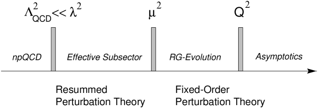
Figure 2.: Regimes of chromodynamics characterized by scales typical for the quanta involved.

The ambiguities parameterized by the scheme constants $C_{i}$ emerge from the truncation of the perturbative series and would be absent if one was able to derive all-order expressions in the coupling constant. In fact, the calculated (pion) form factor depends implicitly on both scales: the adopted renormalization scale via $\alpha_{\rm s}$, and the particular factorization scheme through the anomalous dimensions. Since the latter also depend on $\alpha_{\rm s}$, the factorization-scheme and the renormalization-scheme dependences are correlated. On the other hand, the physical form factor is independent of such artificial scales and satisfies $\mu\frac{dF_{\pi}^{\rm phys}\left(Q^{2}\right)}{d\mu}=0$, for $\mu$ being any internal scale. Obviously, both scheme dependences should be treated simultaneously and be minimized in order to improve the self-consistency of the perturbative treatment. In order to render the perturbative prediction reliable, the parameters $C_{i}$ should be adjusted in such a way, as to minimize the influence of higher-order corrections, thus resolving the scheme ambiguity. However, in the present investigation we are not going to explicitly match the fixed-order NLO contributions with the corresponding terms in the re-summed expression for the “soft” logarithms. Available calculations [24, 25, 26, 27] of the NLO contribution to the hard-scattering amplitude for the pion form factor do not include the $k_{\perp}$ components of the gluon propagators, making such a task difficult for the moment. Instead, we are going to show in Sect. 5 that a potential double counting of re-summed and NLO contributions is de facto very small and of no real practical importance, especially in view of the poor quality of the existing experimental data. In addition, to limit a possible double counting as far as possible, we have meticulously restricted the numerical evaluation of our analytic expressions to the appropriate kinematical regimes.

In Eq. (15), $T_{\rm H}$ is the amplitude for a quark and an anti-quark to scatter via a series of hard-gluon exchanges with gluonic transverse momenta (alias inter-quark transverse distances) not neglected from the outset. To leading order in the running coupling, one has

$$T_{\rm H}\left(x,y,b,Q;\mu_{\rm R}\right)=8C_{\rm F}\alpha_{\rm s}^{{\rm an}}(\mu_{\rm R}^{2})K_{0}\left(\sqrt{xy}\,bQ\right)\;.$$ (18)

This result is related to the more familiar momentum-space expression

$$T_{\rm H}\left(x,y,{\bf k}_{\perp},{\bf l}_{\perp},Q,\mu_{\rm R}\right)=\frac{16\pi\,C_{\rm F}\,\alpha_{\rm s}(\mu_{\rm R}^{2})}{xyQ^{2}+\left({\bf k}_{\perp}+{\bf l}_{\perp}\right)^{2}}$$ (19)

via the Fourier transformation

$$T_{\rm H}\left(x,y,{\bf k}_{\perp},{\bf l}_{\perp},Q,\mu_{\rm R}\right)=\int_{-\infty}^{\infty}d{}^{2}{\bf b}_{\perp}\,T_{\rm H}\left(x,y,b,Q,\mu_{R}\right)\exp\left[i{\bf b}_{\perp}\cdot\left({\bf k}_{\perp}+{\bf l}_{\perp}\right)\right]\;,$$ (20)

where use of the symmetry of $\psi_{\pi}$ under $x\leftrightarrow 1-x\equiv\bar{x}$ has been made, and where $C_{\rm F}=(N_{\rm c}^{2}-1)/2N_{\rm c}=4/3$ for $SU(3)_{\rm c}$. In the limit $Q^{2}\to\infty$ (and $x$ fixed) this expression coincides with the asymptotic hard scattering in the collinear approximation, up to suppressed power corrections. The latter become important in the end-point region ($x\to 0$) at fixed $Q^{2}$, where the actual momentum flow in the gluon propagator becomes small (typically of the order of $\Lambda_{\rm QCD}$) so that gluonic transverse momenta cannot be safely neglected.

The amplitude

$${\cal P}_{\pi}\left(x,b,P\simeq Q,C_{1},C_{2},\mu\right)=\exp\Biggl{[} -s\left(x,b,Q,C_{1},C_{2}\right)-s\left(\bar{x},b,Q,C_{1},C_{2}\right)$$ (22)

$$-2\int_{C_{1}/b}^{\mu}\frac{d\bar{\mu}}{\bar{\mu}}\,\gamma_{q}\left(\alpha_{\rm s}^{\rm an}(\bar{\mu})\right)\Biggr{]}{\cal P}_{\pi}\left(x,b,C_{1}/b\right)$$

describes the distribution of longitudinal momentum fractions of the qq̄ pair, taking into account the intrinsic transverse size of the pion state [30] and comprising corrections due to soft real and virtual gluons [29], including also evolution from the initial amplitude ${\cal P}_{\pi}\left(x,b,C_{1}/b\right)$ at point $C_{1}/b$ to the renormalization scale $\mu\propto Q$. Let us emphasize at this point that the power-behaved term, $\alpha^{\rm npert}$, does not change the leading double logarithmic behavior of the Sudakov exponent. The main effect of the absence of a Landau pole in the running coupling $\alpha_{\rm s}^{\rm an}$ is to make the functions $s\left(x,b,Q,C_{1},C_{2}\right)$, $s\left(\bar{x},b,Q,C_{1},C_{2}\right)$ well-defined (analytic) in the IR region and to slow down evolution by extending soft-gluon cancellation down to the scale $C_{1}/b\simeq\Lambda_{\rm QCD}$, where the full Sudakov form factor acquires a finite value, modulo its $Q^{2}$ dependence (see Fig. 3). In addition, as we shall see below, the Sudakov exponent contains power-behaved corrections in $\left(C_{1}/b\Lambda\right)^{2p}$ and $\left(C_{2}/\xi Q\Lambda\right)^{2p}$, starting with $p=1$. Such contributions are the footprints of soft gluon emission at the kinematic boundaries to the non-perturbative QCD regime, characterized by the transversal (or IR) and the longitudinal (or collinear) cutoffs.

The pion distribution amplitude evaluated at the (low) factorization scale $C_{1}/b$ is approximately given by

$${\cal P}_{\pi}\left(x,b,C_{1}/b,m_{\rm q}\right)\simeq\frac{f_{\pi}/\sqrt{2}}{2\sqrt{N_{\rm c}}}\,\phi_{\pi}\left(x,C_{1}/b\right)\Sigma\left(x,b,m_{\rm q}\right)\;.$$ (23)

Because we retain the intrinsic transverse momenta of the pion bound state, we have to make an ansatz for their distribution. In the present work, we follow Brodsky, Huang, and Lepage [28] (see, also [30, 47]) and parameterize the distribution $\Sigma(x,{{\bf k}_{\perp}},m_{\rm q})$ in the intrinsic transverse momentum $k_{\perp}$ (or equivalently the intrinsic inter-quark transverse distance $b$) in the form of a non-factorizing in the variables $x$ and $k_{\perp}$ (or $x$ and $b$) Gaussian function, so that

$$\Psi_{\pi}\left(x,{{\bf k}_{\perp}},C_{1}/b,m_{\rm q}\right)=\frac{f_{\pi}/\sqrt{2}}{2N_{\rm c}}\Phi_{\pi}(x,C_{1}/b)\Sigma\left(x,{{\bf k}_{\perp}},m_{\rm q}\right)\;,$$ (24)

where

$$\Phi_{\pi}\left(x,C_{1}/b\right)=A\,\Phi_{\rm as}(x)=A\,6x(1-x)$$ (25)

is the asymptotic distribution amplitude, with $A$ being an appropriate normalization factor, and where

$$\Sigma\left(x,{{\bf k}_{\perp}},m_{\rm q}\right)=16\pi^{2}\beta^{2}g(x)\hat{\Sigma}\left(x,{{\bf k}_{\perp}}\right)\hat{\Sigma}\left(x,m_{\rm q}\right)$$ (26)

with

$$\hat{\Sigma}\left(x,{{\bf k}_{\perp}}\right)=\exp{\left[-\beta^{2}{{\bf k}_{\perp}}^{2}g(x)\right]}\;,$$ (27)

and

$$\hat{\Sigma}\left(x,m_{\rm q}\right)=\exp{\left[-\beta^{2}m_{\rm q}^{2}g(x)\right]}\;,$$ (28)

models the distribution in the intrinsic transverse momentum in the form of a Gaussian in the sense of the BHL ansatz.

Neglecting transverse momenta in Eq. (19) (collinear approximation), the only dependence on $k_{\perp}$ resides in the wave function. Furthermore, limiting the maximum value of $k_{\perp}$, these degrees of freedom can be integrated out independently for the initial and final pion states to give way to the corresponding pion distribution amplitudes, which depend only implicitly on the cutoff momentum $\mu^{2}=\left(C_{1}/b\right)^{2}$:

$$\frac{f_{\pi}/\sqrt{2}}{2\sqrt{N_{\rm c}}}\,\phi_{\pi}\left(x,C_{1}/b\right)=\int^{\left(C_{1}/b\right)^{2}}\frac{d^{2}{\bf k}_{\perp}}{16\pi^{3}}\,\Psi_{\pi}\left(x,{{\bf k}_{\perp}},m_{\rm q}\right)\;,$$ (29)

where $f_{\pi}=130.7$ MeV and $N_{\rm c}=3$. Setting $g(x)=1/\left(x(1-x)\right)$ and integrating on both sides of this equation over $x$, supplies us with the constraint

$$1=A\int_{0}^{1}dx6x(1-x)\exp{\left[-\frac{\beta^{2}m_{\rm q}^{2}}{x(1-x)}\right]}$$ (30)

because by virtue of the leptonic decay $\pi\rightarrow\mu^{+}\nu_{\mu}$ the rhs of Eq. (29) is fixed to $\frac{f_{\pi}/\sqrt{2}}{2\sqrt{N_{\rm c}}}$, so that

$$\int_{0}^{1}dx\,\phi_{\pi}\left(x,\mu^{2},m_{\rm q}=0\right)=1$$ (31)

and

$$\int\frac{d{}^{2}{{\bf k}_{\perp}}}{16\pi^{3}}\hat{\Sigma}\left(x,{{\bf k}_{\perp}}\right)=1$$ (32)

for any factorization (normalization) scale $\mu$. The contributions from higher Fock states are of higher twist and contribute corrections at higher order in $1/Q$, i.e., they are power-law suppressed.

Moreover, from $\pi^{0}\to\gamma\gamma$, we have

$$1=8Af_{\pi}^{2}\pi^{2}\beta^{2}\int_{0}^{1}dx\exp{\left[-\frac{\beta^{2}m_{\rm q}^{2}}{x(1-x)}\right]}\;,$$ (33)

while the quark probability $P_{\rm{q\bar{q}}}$ and the average transverse momentum $\langle{{\bf k}_{\perp}}^{2}\rangle$ are given by

$$P_{\rm{q\bar{q}}}=12A^{2}f_{\pi}^{2}\pi^{2}\beta^{2}\int_{0}^{1}dxx(1-x)\exp{\left[-\frac{2\beta^{2}m_{\rm q}^{2}}{x(1-x)}\right]}\;,$$ (34)

$$\langle{{\bf k}_{\perp}}^{2}\rangle=\frac{6A^{2}f_{\pi}^{2}\pi^{2}}{P_{\rm{q\bar{q}}}}\int_{0}^{1}dxx^{2}(1-x)^{2}\exp{\left[-\frac{2\beta^{2}m_{\rm q}^{2}}{x(1-x)}\right]}\;.$$ (35)

By inputting $f_{\pi}$ and the value of the quark mass $m_{\rm q}$, we determine the parameters $A$, $\beta^{2}$, $P_{\rm{q\bar{q}}}$, and ${\langle{{\bf k}_{\perp}}^{2}\rangle}^{1/2}$ (see, Table 1).

Table 1.: Values of parameters entering the pion wave function, using the notations of [30]. The values in parentheses refer to the case $m_{\rm q}=0$. Here the subscript as on $\beta^{2}$ refers to the asymptotic distribution amplitude.

Input parameters	Determined parameters
$m_{\rm q}=0.33$ GeV	$A=\frac{1}{6}\cdot 10.01$ $(\frac{1}{6}\cdot 6)$
$f_{\pi}=0.1307$ GeV	$\beta_{\rm as}^{2}=0.871$ GeV-2 $(0.743$ GeV${}^{-2})$
	${\langle{{\bf k}_{\perp}}^{2}\rangle}^{1/2}=0.352$ GeV $(0.367$ GeV)
	$P_{\rm{q\bar{q}}}=0.306$ $(0.250)$

How large should be the quark mass used in the BHL ansatz? The parameter $m_{\rm q}$ has not the meaning of a real mechanical mass for the quark, but reflects the complicated structure of the QCD vacuum. Let us make this point more transparent. The QCD Lagrangian contains no mass scale in the chiral limit. A mass scale enters perturbatively only through dimensional transmutation to enable renormalization. Nonperturbative scales derive from vacuum fluctuations of some definite correlation length in the context of specified QCD vacuum models. For instance, in the chiral quark model derived from the instanton approach ([52, 53]), the pivotal nonperturbative scale is the average instanton size $\rho$, whose inverse defines a mass scale of the order of $0.600$ GeV. Breaking chiral symmetry spontaneously in the instanton vacuum by the delocalization of the fermionic zero modes, the massless quark acquires a momentum-dependent mass to become a quasi-particle. The obtained value of this effective mass in the quark propagator is $M\sim\rho/R^{2}\simeq 0.300-0.350$ GeV, where $R$ denotes the separation between the quark and the antiquark. Note that though one deals with massive quarks, higher Fock states are not necessarily zero, as the quark propagator contains a renormalization factor $Z\sim 1+O(\rho^{2}/R^{2})$ from which one infers that parton quarks and the “constituent” quarks (the quasi-particles) of this model are equal at leading order in the small parameter $\rho^{2}/R^{2}$. Hence, on the basis of the nonperturbative structure of the QCD vacuum, we may conclude that the mass scale characterizing the quarks in the pion is of the order of the typical constituent quark mass. Then, it seems plausible to set the mass scale $m_{\rm q}$ in the BHL ansatz equal to the dynamical mass $M_{\rm q}$ obtained in such a nonperturbative vacuum model, rather than to use a current quark mass of a few MeV. Only for a very dilute instanton vacuum one can realize $M_{\rm q}\ll\rho^{-1}$, but then the shape of the pion distribution amplitude deviates significantly from the asymptotic one becoming very flat. Actually, one may considerably simplify the BHL ansatz by setting all scales responsible for the intrinsic (transverse) structure of the hadron (the pion), namely ${\langle{{\bf k}_{\perp}}^{2}\rangle}^{1/2}$ and $m_{\rm q}$ equal to $\Lambda_{\rm QCD}$ which is of the same order of magnitude: $0.200-0.350$ GeV. Indeed, the predictions obtained with this simplification are close to those calculated with the values given in Table 1.

Let us now return to Eq. (22). The Sudakov form factor $F_{\rm S}\left(\xi,b,Q,C_{1},C_{2}\right)$, i.e., the exponential factor in front of the wave function, will be expressed as the expectation value of an open Wilson (world) line along a contour of finite extent, $C$, which follows the bent quark line in the hard-scattering process from the segment with direction $P$ to that with direction $P^{\prime}$ after being abruptly derailed by the hard interaction which creates a “cusp” in $C$, and is to be evaluated within the range of momenta termed “soft”, confined within the range limited by $C_{1}/b$ (IR cutoff) and $C_{2}\xi Q$ (longitudinal cutoff) (where $\xi=x,\bar{x},y,\bar{y}$). Thus we have [37, 38, 39, 40, 54]

$$F_{\rm S}\left(W(C)\right)=\left\langle{\rm P}\exp\left(ig\int_{C}dz\cdot t^{a}A^{a}(z)\right)\right\rangle_{\rm soft}\;,$$ (36)

where P stands for path ordering along the integration contour $C$, and where ${<...>}_{A}$ denotes functional averaging in the gauge field sector with whatever this may entail (ghosts, gauge choice prescription, Dirac determinant, etc.). Having isolated a sub-sector of the full theory (cf. Fig. 2), where only gluons with virtualities between $C_{1}/b$ and $C_{2}\xi Q$ are active degrees of freedom, quark propagation and gluon emission can be described by eikonal techniques, using either Feynman diagrams [42, 32] or by employing a world-line casting of QCD which reverts the fermion functional integral into a first-quantized, i.e., particle-based path integral [40].

Then the Sudakov functions, entering Eq. (22), can be expressed in terms of the momentum-dependent cusp anomalous dimension of the bent contour to read

$$s\left(\xi,b,Q,C_{1},C_{2}\right)=\frac{1}{2}\int_{C_{1}/b}^{C_{2}\xi Q}\frac{d\mu}{\mu}\,\Gamma_{{\rm cusp}}\left(\gamma,\alpha_{\rm s}^{\rm an}(\mu)\right)$$ (37)

with the anomalous dimension of the cusp given by

$$\Gamma_{{\rm cusp}}\left(\gamma,\alpha_{\rm s}^{\rm an}(\mu)\right) = 2\ln\left(\frac{C_{2}\xi Q}{\mu}\right)A\left(\alpha_{\rm s}^{\rm an}(\mu)\right)+B\left(\alpha_{\rm s}^{\rm an}(\mu)\right)\;,$$ (38)

$$\equiv \Gamma_{{\rm cusp}}^{\rm pert}+\Gamma_{{\rm cusp}}^{\rm npert}\;,$$ (39)

$\gamma=\ln\left(C_{2}\xi Q/\mu\right)$ being the cusp angle, i.e., the emission angle of a soft gluon and the bent eikonalized quark line after the external (large) momentum $Q$ has been injected at the cusp point by the off-mass-shell photon, and where in the second line of Eq. (39) the superscripts relate to the origin of the corresponding terms in the running coupling (cf. Eqs. (2), (3)). The functions $A$ and $B$ are known at two-loop order:

$$A\left(\alpha_{\rm s}^{\rm an}(\mu)\right) = \frac{1}{2}\left[\gamma_{\cal K}\left(\alpha_{\rm s}^{\rm an}(\mu)\right)+\beta(g)\frac{\partial}{\partial g}{\cal K}(C_{1},\alpha_{\rm s}^{\rm an}(\mu))\right]$$ (40)

$$= C_{\rm F}\frac{\alpha_{\rm s}^{\rm an}(g(\mu))}{\pi}+\frac{1}{2}K\left(C_{1}\right)C_{\rm F}\left(\frac{\alpha_{\rm s}^{\rm an}(g(\mu))}{\pi}\right)^{2}\;,$$ (41)

and

$$B\left(\alpha_{\rm s}^{\rm an}(\mu)\right) = -\frac{1}{2}\left[{\cal K}\left(C_{1},\alpha_{\rm s}^{\rm an}(\mu)\right)+{\cal G}\left(\xi,C_{2},\alpha_{\rm s}^{\rm an}(\mu)\right)\right]$$ (42)

$$= \frac{2}{3}\frac{\alpha_{\rm s}^{\rm an}(g(\mu))}{\pi}\ln\left(\frac{C_{1}^{2}}{C_{2}^{2}}\frac{{\rm e}^{2\gamma_{E}-1}}{4}\right)\;.$$ (43)

The first term in Eq. (41) is universal, while the second one as well as the contribution termed $B$ are scheme dependent. The K-factor in the ${\overline{\rm MS}}$ scheme to two-loop order is given by [37, 38, 42, 43, 55]

$$K\left(C_{1}\right)=\left(\frac{67}{18}-\frac{\pi^{2}}{6}\right)C_{\rm A}-\frac{10}{9}n_{\rm f}T_{\rm F}+\beta_{0}\ln\left(C_{1}{\rm e}^{\gamma_{\rm E}}/2\right)$$ (44)

with $C_{\rm A}=N_{\rm C}=3$, $n_{\rm f}=3$, $T_{\rm F}=1/2$, and $\gamma_{\rm E}$ being the Euler-Mascheroni constant.

The quantities ${\cal K}$, ${\cal G}$ in Eq. (43) are calculable using the non-Abelian extension to QCD [42] of the Grammer-Yennie method [56] for QED. Alternatively, one can calculate the cusp anomalous dimension employing Wilson (world) lines [38, 39, 40, 54]. In this latter approach (see, e.g., [40]), the IR behavior of the cusped Wilson (world) line is expressed in terms of an effective fermion vertex function whose variance with the momentum scale is governed by the anomalous dimension of the cusp within the isolated effective sub-sector (see Fig. 2). Since this scale dependence is entirely restricted within the low-momentum sector of the full theory, IR scales are locally coupled and the soft (Sudakov-type) form factor depends only on the cusp angle which varies with the inter-quark transverse distance $b$ ranging between $C_{1}/b$ and $C_{2}\xi Q$.

The corresponding anomalous dimensions are linked to each other (for a nice discussion, see [37]) through the relation $2\Gamma_{{\rm cusp}}\left(\alpha_{\rm s}^{\rm an}(\mu)\right)=\gamma_{\cal K}\left(\alpha_{\rm s}^{\rm an}(\mu)\right)$ with $\Gamma_{{\rm cusp}}(\alpha_{\rm s}^{\rm an}(\mu))=C_{\rm F}\,\alpha_{\rm s}^{\rm an}(\mu^{2})/\pi$, which shows that $\frac{1}{2}\gamma_{\cal K}=A\left(\alpha_{\rm s}^{\rm an}(\mu)\right)$. (Note that $\gamma_{\cal G}=-\gamma_{\cal K}$.)

The soft amplitude ${\cal P}_{\pi}\left(x,b,C_{1}/b,\mu\right)$ and the hard-scattering amplitude $T_{\rm H}\left(x,y,b,Q,\mu\right)$ satisfy independent RG equations to account for the dynamical factorization (recall that both $b$ and $\xi$ are integration variables) with solutions controlled by the power-term modified “evolution time” (see, e.g., [51] and earlier references cited therein):

$$\tau\left(\frac{C_{1}}{b},\mu\right) = \int_{C_{1}^{2}/b^{2}}^{\mu^{2}}\frac{dk^{2}}{k^{2}}\,\frac{\alpha_{\rm s}^{{\rm an}(1)}(k^{2})}{4\pi}$$ (45)

$$= \frac{1}{\beta_{0}}\ln\frac{\ln\left(\mu^{2}/\Lambda^{2}\right)}{\ln\left(C_{1}^{2}/\left(b\Lambda\right)^{2}\right)}+\frac{1}{\beta_{0}}\left[\ln\frac{\mu^{2}}{\left(C_{1}/b\right)^{2}}-\ln\frac{\left|\mu^{2}-\Lambda^{2}\right|}{\left|\frac{C_{1}^{2}}{b^{2}}-\Lambda^{2}\right|}\right]$$ (46)

from the factorization scale $C_{1}/b$ to the observation scale $\mu$, with $\Lambda$ denoting $\Lambda_{\rm QCD}$ as before. The evolution time is directly related to the quark anomalous dimension, viz., $\gamma_{\rm q}\left(\alpha_{\rm s}^{\rm an}(\mu)\right)=-\alpha_{\rm s}^{{\rm an}}(\mu^{2})/\pi$. One appreciates that the second term in (46) stems from the power-generated correction to the running coupling, $\alpha_{\rm s}^{\rm npert}$, and is absent in the conventional approach. At moderate values of $\mu^{2}$ this term is “slowing down” the rate of evolution.

The leading contribution to the IR-modified Sudakov functions $s\left(\xi,b,Q,C_{1},C_{2}\right)$ (where $\xi=x,\bar{x},y,\bar{y}$) is obtained by expanding the functions $A$ and $B$ in a power series in $\alpha_{\rm s}^{\rm an}$ and collecting together all large logarithms $\left(\frac{\alpha_{\rm s}^{\rm an}}{\pi}\right)^{n}\ln\left(\frac{C_{2}}{C_{1}}\xi bQ\right)^{m}$, which can be transformed back into large logarithms $\ln\left(Q^{2}/{{\bf k}_{\perp}}^{2}\right)$ in transverse momentum space. Employing equations (2) and (3), the leading contribution results from the expression

$$s\left(\xi,b,Q,C_{1},C_{2}\right)= \frac{1}{2}\int_{C_{1}/b}^{C_{2}\xi Q}\frac{d\mu}{\mu}\Biggl{\{}2\ln\left(\frac{C_{2}\xi Q}{\mu}\right)\Biggl{[}\frac{\alpha_{\rm s}^{{\rm an}(2)}(\mu)}{\pi}A^{(1)}+\left(\frac{\alpha_{\rm s}^{{\rm an}(1)}(\mu)}{\pi}\right)^{2}A^{(2)}\left(C_{1}\right)\Biggr{]}$$ (48)

$$+\frac{\alpha_{\rm s}^{{\rm an}(1)}(\mu)}{\pi}B^{(1)}\left(C_{1},C_{2}\right)+{\cal O}\left(\frac{\alpha_{\rm s}^{\rm an}}{\pi}\right)^{3}\Biggr{\}}\;,$$

where Eq. (3) is to be used in front of $A^{(1)}$, whereas the other two terms are to be evaluated with Eq. (2). The specific values of the coefficients $A^{(i)}$, $B^{(i)}$ are

$$A^{(1)} = C_{\rm F}\;,$$ (49)

$$A^{(2)}\left(C_{1}\right) = \frac{1}{2}\,C_{\rm F}\,K\left(C_{1}\right)\;,$$ (50)

$$B^{(1)}\left(C_{1},C_{2}\right) = \frac{2}{3}\ln\left(\frac{C_{1}^{2}}{C_{2}^{2}}\frac{{\rm e}^{2\gamma_{E}-1}}{4}\right)\;,$$ (51)

in which the term proportional to $A^{(1)}$ represents the universal part. As now the power-correction term in $\alpha_{\rm s}^{\rm an}$ gives rise to poly-logarithms, a formal analytic expression for the full Sudakov form factor is too complicated for being presented. We only display the universal contribution in LLA:

$$F_{\rm S}^{\rm univ}\left(\mu_{\rm F},Q\right)= \exp\Biggl{\{}-\frac{C_{\rm F}}{\beta_{0}}\Biggl{[}\ln\left(\frac{\tilde{Q}^{2}}{\Lambda^{2}}\right)\ln\frac{\ln\tilde{Q}^{2}/\Lambda^{2}}{\ln\mu_{\rm F}^{2}/\Lambda^{2}}-\ln\frac{\tilde{Q}^{2}}{\mu_{\rm F}^{2}}$$ (53)

$$+\ln\left(\frac{\tilde{Q}^{2}}{\mu_{\rm F}^{2}}\right)\ln\frac{{\Lambda}^{2}-\mu_{\rm F}^{2}}{\Lambda^{2}}+\frac{1}{2}\,\ln^{2}\frac{\tilde{Q}^{2}}{\mu_{\rm F}^{2}}+{\rm Li}_{2}\left(\frac{\tilde{Q}^{2}}{\Lambda^{2}}\right)-{\rm Li}_{2}\left(\frac{\mu_{\rm F}^{2}}{\Lambda^{2}}\right)\Biggr{]}\Biggl{\}}\;,$$

where $\tilde{Q}$ represents the scale $C_{2}\xi Q$ and the IR matching (factorization) scale $\mu_{\rm F}$ varies with the inverse transverse distance $b$, i.e., $\mu_{\rm F}=C_{1}/b$. Note that the four last terms in this equation originate from the non-perturbative power correction (cf. Eq. (39)), and that ${\rm Li}_{2}$ is the dilogarithm (Spence) function which comprises power-behaved corrections of the IR ($b\Lambda$) and the longitudinal ($Q/\Lambda$) cutoff scales. In the calculations to follow, Eq. (48) is evaluated numerically to NLLA with appropriate kinematic bounds to ensure proper factorization at the numerical level. Above (see Eq. (48)), we have replaced $\left(\alpha_{\rm s}^{(1)}\right)^{2}$ by $\left(\alpha_{\rm s}^{{\rm an}(1)}\right)^{2}$. Here we have an analytization ambiguity. Since nonlinear relations are not preserved by the analytization procedure [57] (see, also [11]), we could have made the square of the running coupling, $\left(\alpha_{\rm s}^{(1)}\right)^{2}$, analytic as a whole. We plan to report on these interesting conceptual issues of analytization in a separate publication.

Note that, neglecting the power-generated logarithms, we obtain an equation for the conventional Sudakov function, which we write as an expansion in inverse powers of the first beta-function coefficient $\beta_{0}$ to read

$$s\left(\xi,b,Q,C_{1},C_{2}\right)= \frac{1}{\beta_{0}}\left[\left(2A^{(1)}\hat{Q}+B^{(1)}\right)\ln\frac{\hat{Q}}{\hat{b}}-2A^{(1)}\left(\hat{Q}-\hat{b}\right)\right]$$ (56)

$$-\,\frac{4}{\beta_{0}^{2}}A^{(2)}\left(\ln\frac{\hat{Q}}{\hat{b}}-\frac{\hat{Q}-\hat{b}}{\hat{b}}\right)$$

$$+\frac{\beta_{1}}{\beta_{0}^{3}}A^{(1)}\left\{\ln\frac{\hat{Q}}{\hat{b}}-\frac{\hat{Q}-\hat{b}}{\hat{b}}\left[1+\ln\left(2\hat{b}\right)\right]+\frac{1}{2}\left[\ln^{2}\left(2\hat{Q}\right)-\ln^{2}\left(2\hat{b}\right)\right]\right\}\;,$$

where the convenient abbreviations [29] $\hat{Q}\equiv\ln\frac{C_{2}\xi Q}{\Lambda}$ and $\hat{b}\equiv\ln\frac{C_{1}}{b\Lambda}$ have been used.

This quantity differs from the original result given by Li and Sterman in [29], and, though it almost coincides numerically with the formula derived by J. Bolz [58], it differs from that algebraically.

All told, the final expression for the electromagnetic pion form factor at leading perturbative order in $T_{\rm H}$ and next-to-leading logarithmic order in the Sudakov form factor has the form

$$F_{\pi}(Q^{2})= \frac{2}{3}\,A^{2}\pi\,C_{\rm F}\,f_{\pi}^{2}\,\int_{0}^{1}dx\int_{0}^{1}dy\int_{0}^{\infty}b\,db\,\alpha_{\rm s}^{{\rm an}(1)}\left(\mu_{\rm R}\right)\Phi_{\rm as}(x)\Phi_{\rm as}(y)\exp\left[-\frac{b^{2}\left(x\bar{x}+y\bar{y}\right)}{4\beta_{\rm as}^{2}}\right]$$ (58)

$$\times\exp{\left[-\beta_{\rm as}^{2}m_{\rm q}^{2}\left(\frac{1}{x\bar{x}}+\frac{1}{y\bar{y}}\right)\right]}K_{0}\left(\sqrt{xy}Qb\right)\exp\left[-S\left(x,y,b,Q,C_{1},C_{2},C_{4}\right)\right]\;,$$

where

$$S\left(x,y,b,Q,C_{1},C_{2},C_{4}\right)\equiv s\left(x,b,Q,C_{1},C_{2}\right)+s\left(\bar{x},b,Q,C_{1},C_{2}\right)+(x\leftrightarrow y)-8\,\tau\left(\frac{C_{1}}{b},\mu_{\rm R}\right)$$ (59)

with $\tau\left(C_{1}/b,\mu_{\rm R}\right)$ given by Eq. (46) and $\mu_{\rm R}=C_{4}f(x,y)Q$. As we shall show below, the effect of including the effective quark mass in the hard part of the form factor is almost negligible, as one should expect on theoretical grounds.

Before we go beyond the leading order in the perturbative expansion of the hard-scattering amplitude, $T_{\rm H}$, let us pause for a moment to comment on the pion wave function. We have pro-actively indicated in Eq. (58) that the asymptotic distribution amplitude $\Phi_{\rm as}(x)=6x\bar{x}$ will be used.

A few words about this choice are now in order.

Hadron wave functions are clearly the essential variables needed to model and describe the properties of an intact hadron. In the past, most attempts to improve the theoretical predictions for the hard contribution to the pion form factor have consisted of using end-point concentrated wave functions (distribution amplitudes). In this analysis we refrain from using such distribution amplitudes of the Chernyak-Zhitnitsky (CZ) type [59], referring for a compilation of objections and references to [22] (see also [60]), and present instead evidence for an alternative source of enhancement due to the non-perturbative power correction in the running coupling.

This IR-enhancement effect was found in [22] to be quite significant, even for the asymptotic solution (to the evolution equation) which has its maximum at $x=1/2$. Indeed, the IR-enhanced hard contribution can account already at leading perturbative order for a sizable part of the measured magnitude of the electromagnetic pion form factor, though agreement with the currently available experimental (low-momentum) data calls for the inclusion of the soft, non-factorizing contribution (cf. Eq. (12)) [61, 62, 63, 47] – even if the NLO correction is taken into account (see Sect. 5). Nevertheless, the true pion distribution amplitude may well be a “hybrid” of the type $\Phi_{\pi}^{\rm true}=90\%\Phi_{\pi}^{\rm as}+9\%\Phi_{\pi}^{\rm CZ}+1\%C_{4}^{(3/2)}$, where the mixing ensures a broader shape with the fourth-order, “Mexican hat”-like, Gegenbauer polynomial $C_{4}^{(3/2)}$, being added in order to cancel the dip of $\Phi_{\rm CZ}$ at $x=1/2$.

First tasks from instanton-based approaches show that the extracted pion distribution amplitudes are very close to, albeit somewhat broader than, the asymptotic form [64, 65, 66]. Similar results were also obtained using nonlocal condensates [67, 68]. The discussion of non-asymptotic pion distribution amplitudes will be conducted elsewhere.

4 Pion form factor to order $\left(\alpha_{\rm s}^{\rm an}(Q^{2})\right)^{2}$

Next, we generalize our calculation of the hard contribution to the pion form factor by taking into account the perturbative correction to $T_{\rm H}$ of order $\alpha_{\rm s}^{2}$, using the results obtained in [24, 25, 26, 27], in combination with our analytical, i.e., IR-finite (IRF) factorization and renormalization scheme.

To be precise, we only include the NLO corrections to $T_{\rm H}$, leaving NLO corrections to the evolution of the pion distribution amplitude aside. The reason is that for the asymptotic distribution amplitude, at issue here, these corrections are tiny, appearing first at NLO [69, 27]. For sub-asymptotic distribution amplitudes, however, evolutional corrections [69] have to be taken into account. Strictly speaking, the calculation below is incomplete, the reason being that the transverse degrees of freedom in the NLO terms of $T_{\rm H}$ have been neglected, albeit the intrinsic ones in the wave functions have been taken into account – in contrast to other approaches [27]. Hence, our prediction should be regarded rather as an upper limit for the size of the hard contribution to the pion form factor than as an exact result. Taking into account the $k_{\perp}$-dependence of $T_{\rm H}$ at NLO, as we did for the leading part, this result might be somewhat reduced as shown for the pion in [30] and for the nucleon in [70] (for a comprehensive discussion of $k_{\perp}$ effects, we refer to [71]), though we expect that due to IR-finiteness, this reduction should be rather small and the quality of our predictions almost unchanged. Note in this context that we always refer to the asymptotic distribution amplitude of the pion. Broadening the pion distribution amplitude would lead to a larger normalization of (form-factor) magnitudes. We would also like to emphasize that other higher-twist contributions of non-perturbative origin, as those mentioned before, may also raise the magnitude of the form factor. However, such contributions are not on the focus of the present work.

Applying these assumptions, Eq. (58) extends to NLO to read

$$F_{\pi}\left(Q^{2}\right) = 16A^{2}\pi C_{\rm F}\left(\frac{f_{\pi}/\sqrt{2}}{2\sqrt{N_{\rm c}}}\right)^{2}\int_{0}^{1}dx\int_{0}^{1}dy\int_{0}^{\infty}b\,db\,\alpha_{\rm s}^{\rm an}\left(\mu_{\rm R}^{2}\right)\Phi_{\rm as}(x)\Phi_{\rm as}(y)$$ (63)

$$\times\exp\left[-\frac{b^{2}\left(x\bar{x}+y\bar{y}\right)}{4\beta_{\rm as}^{2}}\right]\exp{\left[-\beta_{\rm as}^{2}m_{\rm q}^{2}\left(\frac{1}{x\bar{x}}+\frac{1}{y\bar{y}}\right)\right]}$$

$$\times K\left(\sqrt{xy}Qb\right)\exp\left(-S\left(x,y,b,Q,C_{1},C_{2},C_{4}\right)\right)$$

$$\times\left[1+\frac{\alpha_{\rm s}^{\rm an}}{\pi}\left(f_{\rm UV}\left(x,y,Q^{2}/\mu_{\rm R}^{2}\right)+f_{\rm IR}\left(x,y,Q^{2}/\mu_{\rm F}^{2}\right)+f_{\rm C}(x,y)\right)\right]\;,$$

where the Sudakov form factor, including evolution, is given by Eq. (59), $\mu_{\rm F}=C_{1}/b$, and the functions $f_{i}$ are taken from [27]. They are given by

$$f_{\rm UV}\left(x,y,Q^{2}/\mu_{\rm R}^{2}\right) = \frac{\beta_{0}}{4}\left(\frac{5}{3}-\ln\left(\bar{x}\bar{y}\right)+\ln\frac{\mu_{\rm R}^{2}}{Q^{2}}\right)\;,$$ (64)

$$f_{\rm IR}\left(x,y,Q^{2}/\mu_{\rm F}^{2}\right) = \frac{2}{3}\left(3+\ln\left(\bar{x}\bar{y}\right)\right)\left(\frac{1}{2}\ln\left(\bar{x}\bar{y}\right)-\ln\frac{\mu_{\rm F}^{2}}{Q^{2}}\right)\;,$$ (65)

$$f_{\rm C}(x,y) = \frac{1}{12}\left[-34+12\ln\left(\bar{x}\bar{y}\right)+\ln x\ln y\right.$$ (68)

$$+\ln\bar{x}\ln\bar{y}-\ln x\ln\bar{y}-\ln\bar{x}\ln y$$

$$\left.+(1-x-y)H(x,y)+R(x,y)\right]$$

and are related to UV and IR poles, as indicated by corresponding subscripts, that have been removed by dimensional regularization along with the associated constants $\ln(4\pi)-\gamma_{\rm E}$, whereas $f_{\rm C}(x,y)$ is scale-independent. In evaluating expression $f_{\rm C}$ in (68), we found it particularly convenient to use the representation of the function $H(x,y)$ given by Braaten and Tse [26],

$$H(x,y)=\frac{1}{1-x-y}\left[{\rm Li}_{2}(\bar{x})+{\rm Li}_{2}(\bar{y})-{\rm Li}_{2}(x)-{\rm Li}_{2}(y)+\ln x\ln y-\ln\bar{x}\ln\bar{y}\right]\;,$$ (69)

where again ${\rm Li}_{2}$ denotes the dilogarithm function. For the function $R(x,y)$ we have used the expression derived by Field et al. [24], except at point $x\approx y$, where we employed the Taylor expansion displayed below:

$$R(x,y) = \frac{1}{3\,\left(-1+y\right)\,y^{2}}\Bigl{[}\left(-1+33\,y-45\,y^{2}+13\,y^{3}\right)\,\ln\bar{y}$$ (75)

$$\phantom{\frac{1}{3\,\left(-1+y\right)\,y^{2}}}+y\,\left(-1+y+(9-13\,y)\,y\,\ln y\right)\Bigr{]}$$

$$+\frac{x-y}{3\,(-1+y)^{2}\,y^{3}}\Bigl{[}(-1+y)^{2}\,(-1+16\,y)\,\ln\bar{y}$$

$$\phantom{\frac{x-y}{3\,(-1+y)^{2}\,y^{3}}+}+y\,\left(-1+13\,y-12\,y^{2}+2\,y^{2}\,\ln y\right)\Bigl{]}$$

$$+\frac{(x-y)^{2}}{30\,(-1+y)^{3}\,y^{4}}\Bigl{[}(-1+y)^{3}\,\left(9-148\,y+9\,y^{2}\right)\,\ln\bar{y}$$

$$\phantom{\frac{(x-y)^{2}}{30\,(-1+y)^{3}\,y^{4}}+}-y\left(9-148\,y+328\,y^{2}-189\,y^{3}+y^{3}\,(5+9\,y)\,\ln y\right)\Bigr{]}\;.$$

Note that this expression does not reproduce its counterpart in [24]. It must be remarked once again that evaluating Eq. (63) there is an analytization ambiguity similar to that encountered in the calculation of the Sudakov exponent. This question will be addressed elsewhere.

Having developed in detail the theoretical apparatus, let us now turn to the concrete (numerical) calculation of the pion form factor at NLO.

5 Numerical analysis

This section implements factorization on the numerical level, thus providing the bridge between the analytic framework, developed and discussed in the previous sections, and numerical calculations to follow in the subsequent section. This is done by appropriately defining the accessible phase space regions (kinematic integrals) of transverse momenta (or equivalently transverse distances $b$) for gluon emission in each regime, making explicit the inherent kinematical restrictions on the momenta of hard (soft) gluons due to factorization. The numerical analysis below updates and generalizes our previous investigations in Refs. [22, 23].

In order to set up a reliable algorithm for the numerical evaluation of the expressions presented above, we have to ensure that this is done in kinematic regions where use of fixed-order or re-summed perturbation theory is legal. Further, expedient restrictions have to be imposed to avoid double counting of gluon corrections by carefully defining the validity domain of each contribution to the pion form factor, in correspondence with Fig. 2. These kinematic constraints are compiled below.

Kinematic cuts

1. $C_{1}/b>\Lambda_{\rm QCD}$; otherwise the whole Sudakov exponent $\exp(-S)$ (cf. Eq. (59)) is continued to zero because this large-$b$ region is properly taken into account in the wave functions. This condition excludes from the re-summed perturbation theory soft gluons with wavelengths larger than $C_{1}/\Lambda$, which should be treated non-perturbatively. In other words, it ensures the separation (factorization) of the effective sub-sector from the genuine non-perturbative regime (cf. Fig. 2).

2. $C_{2}\xi Q>C_{1}/b$; otherwise each Sudakov exponent $\exp\left[-s\left(\xi,b,Q,C_{1},C_{2}\right)\right]$ in Eq. (59) is “frozen” to unity because this small-$b$ region is dominated by low orders of perturbation theory rather than by the re-summed perturbation series, and consequently contributions in this region should be ascribed to higher-order corrections to $T_{\rm H}$, which we have taken into account explicitly at NLO. This condition establishes proper factorization between re-summed and fixed-order perturbation theory and helps avoid double counting of such contributions (always working in the gauge $A^{+}=0$). Yet evolution is taken into account to match the scales in our “gliding” factorization scheme.

3. $C_{4}f(x,y)Q>C_{1}/b$; otherwise the evolution time $\tau\left(C_{1}/b,\mu_{\rm R}\right)$ in Eq. (59) is contracted to zero, i.e., evolution is “frozen”. The renormalization scale should be at least equal to the factorization scale, so that the running coupling has always arguments in the range controlled by (re-summed or fixed-order) perturbation theory.

4. $C_{4}f(x,y)Q>C_{2}\xi Q$; otherwise evolution to that scale is “frozen” because this region is appropriately accounted for by the Sudakov contribution. This helps avoiding double counting of terms which belong to the re-summed rather than to the fixed-order perturbation theory. (No overlap at the boundary characterized by the scale $\mu^{2}$ in Fig. 2).

5. $C_{4}f(x,y)Q>C_{1}/b$; otherwise the two scales $\mu_{\rm R}=\mu_{\rm F}=C_{1}/b$ are identified in the function $f_{\rm UV}(x,y)$ (by the same reasoning as above). If $\mu_{\rm R}\leq\Lambda_{\rm QCD}$, then $f_{\rm UV}(x,y)$ is set equal to zero.

6. $C_{1}/b>\Lambda_{\rm QCD}$; otherwise the function $f_{\rm IR}(x,y)$ is set equal to zero. The last two restrictions exclude contributions from perturbative terms when they are evaluated in the non-perturbative kinematic domain.

To illustrate the difference in technology between approaches employing the conventional expression for the full Sudakov exponent [32, 29], on one hand, and our analysis, on the other, we show $\exp(-S)$ graphically in Fig. 3 for three different values of the momentum transfer and $\xi=1/2$. In contrast to Li and Sterman [29], the evolutional contribution is not cut-off at unity, whenever $C_{2}\xi Q<C_{1}/b$. The dotted curve shows the result for Eq. (56) without this cutoff. One infers from this figure that their suggestion to ignore the enhancement due to the anomalous dimension does not apply in our case because the IR-modified Sudakov form factor is not so rapidly decreasing as $b$ increases, owing to the IR-finiteness of $\alpha_{\rm s}^{\rm an}$. Indeed, as $Q$ becomes smaller, $\exp(-S)$ remains constant and fixed to unity for increasing $b$, providing enhancement only in the large-$b$ region before it reaches the kinematic boundary $C_{1}/b=\Lambda_{\rm QCD}$, where it is set equal to zero. As a result, for small $Q$-values, like $Q_{1}=2$ GeV, the enhancement due to the quark anomalous dimension cannot be associated with higher-order corrections to $T_{\rm H}$, since it operates at larger $b$-values, and for that reason it should be taken into account in the Sudakov contribution. Only for asymptotically large $Q$ values, when the IR-modified Sudakov form factor and the conventional one become indistinguishable, the evolutional enhancement becomes a small effect – strictly confined in the small-$b$ region – and can be safely ignored. On the other hand, because the Sudakov exponent is bounded at fixed $Q^{2}$, the Sudakov exponential remains finite until the edge of phase space, $C_{1}/b_{\rm cr}\mathchar 13358\relax\Lambda_{\rm QCD}$, also providing IR enhancement. This behavior is best appreciated by comparing the dashed and dotted curves, both at $Q_{2}=5$ GeV, in Fig. 3.

Figure 3.: Behavior of the Sudakov form factor with respect to the transverse separation $b$ for three representative values of the momentum transfer $Q^{2}$: $Q_{1}=2$ GeV, $Q_{2}=5$GeV, and $Q_{3}=10$ GeV, with all $\xi_{i}=1/2$, and where we have set $C_{1}=2{\rm e}^{-\gamma_{\rm E}}$, $C_{2}={\rm e}^{-1/2}$ and $\Lambda_{\rm QCD}=0.242~{}{\rm GeV}$. The dotted curve shows the result obtained with $\alpha_{\rm s}^{\overline{\rm MS}}$, and $\Lambda_{\rm QCD}=0.2~{}{\rm GeV}$ for $Q_{2}=5$ GeV, using the same set of $C_{i}$ as before. Notice that in this case, evolution is limited by the (renormalization) scale $\mu_{\rm R}=t=\{{\rm max}\sqrt{xy}\,Q,C_{1}/b\}$, as proposed in [29]. However, the enhancement at small $b$-values due to the quark anomalous dimension is not neglected here.

The behavior of the Sudakov form factor, we stress, shows that power-induced sub-leading logarithmic corrections are relevant in the range of currently probed momentum-transfer values. Hence, the advantage of employing such a scheme to calculate hadronic observables, for instance the pion form factor, is that the hard (perturbative) contribution is enhanced, relative to the calculation in the $\overline{\rm MS}$ scheme, and the self-consistency of the perturbative treatment towards lower $Q^{2}$ values, where it is not justified, is significantly improved (no enhancement caused by the Landau obstruction; hence better scaling).

This is because the range in which soft gluons build up the Sudakov form factor is enlarged and inhibition of bremsstrahlung sets in at larger $Q^{2}$. Let us mention in this context that power contributions in the radiative corrections to the meson wave function could lead to suppression of soft gluon emission at large transverse distance $b$. Indeed, Akhoury, Sincovics, and Sotiropoulos [72] have re-summed such power corrections, associated to IR renormalons, with the aid of an effective gluon mass. They found Sudakov-type suppression on top of the Sudakov suppression discussed so far. The discussion of such IR-renormalon-based contributions in conjunction with our IR-finite approach will be presented elsewhere.

6 Phenomenology

Let us now present phenomenological applications of our scheme. Using the techniques discussed above, we obtain for the electromagnetic pion form factor the theoretical predictions shown in Fig. 4. A set of constants $C_{i}$, $(i=1,2,3)$ which eliminate artifacts of dimensional regularization, while practically preserving the matching between the re-summed and the fixed-order calculation, are given in Table 2 in comparison with other common choices of these constants. Moreover, this factorization scale setting enables us to naturally link our scheme to the BLM commensurate scale method [12] in fixing the renormalization scale. Indeed, since the adopted value of $C_{1}$ eliminates both the log term in the $K$-factor (see Eq. (44)), which contains the $\beta$-function, and also the scheme-dependent term $B$ in the cusp anomalous dimension (see Eq. (43)), this choice corresponds to a conformally invariant framework with $\beta_{0}=0$, and therefore connects to the commensurate scale procedure. Hence, we set $C_{4}=C_{2}\exp{(-5/6)}$, which, for our choice of $C_{2}=\exp{(-1/2)}$, rescales $Q$ in the $\overline{\rm MS}$ scheme, we use, by a factor of $\exp{(-4/3)}$. In addition, to avoid large kinematical corrections due to soft gluon emission, we set $f(x,y)=\sqrt{xy}$ to link the renormalization scale to the typical momentum flow in the gluon propagators [55]. In this way, scheme and renormalization scale ambiguities are considerably reduced, as the theoretical predictions are evaluated at a physical momentum scale:

$$\mu_{\rm BLM}=\mu_{\rm R}\exp(-5/6)\;,$$ (76)

where

$$\mu_{\rm R}=C_{4}f(x,y)Q=C_{4}\sqrt{xy}Q\;.$$ (77)

We emphasize, however, that these favored values of the scheme constants by no means restrict the validity of our numerical analysis. They merely indicate the anticipated appropriate choice of the factorization and renormalization scales with respect to observables and theoretical self-consistency. Other choices of these parameters do not change the qualitative features of our predictions.

Table 2.: Different sets of coefficients $C_{i}$ and values of the $K$-factor and the quantity (cf. Eq. (43)) $\kappa=\ln\left(C_{1}^{2}\;{\rm e}^{2\gamma_{E}-1}/4\,C_{2}^{2}\right)$, corresponding to different factorization and renormalization prescriptions. The choice of $C_{4}$ in this work corresponds to BLM-type commensurate scale fixing.

	Scheme parameters $C_{i}$
Choice	$C_{1}$	$C_{2}=\frac{1}{\sqrt{2}}C_{2}^{\rm CSS}$ [42]	$C_{3}$	$C_{4}$	$K$	$\kappa$
canonical	$2\exp\left(-\gamma_{\rm E}\right)$	$1/\sqrt{2}$	$2\exp\left(-\gamma_{\rm E}\right)$	–	4.565	-0.307
SSK [22]	$\exp\left[-\frac{1}{2}\left(2\gamma_{\rm E}-1\right)\right]$	$1/\sqrt{2}$	$\exp\left[-\frac{1}{2}\left(2\gamma_{\rm E}-1\right)\right]$	–	2.827	0
this work	$2\exp\left(-\gamma_{\rm E}\right)$	$\exp\left(-1/2\right)$	$2\exp\left(-\gamma_{\rm E}\right)$	$\exp\left(-4/3\right)$	4.565	0

Figure 4.: Space-like pion form factor calculated within our IR-finite scheme with $\Phi_{\rm as}$ and including an effective (constituent-like) quark mass of $m_{\rm q}=0.33$ GeV in the pion wave function. The broken lines show the IR-enhanced hard contributions obtained with our scheme using commensurate scale setting: LO calculation (dashed-dotted line); NLO calculation (dotted line). The dashed line gives the result for the soft, Feynman-type contribution, computed with $m_{\rm q}=0.33$ GeV in the pion wave function. The solid line represents the sum of the NLO hard contribution and the soft one. The data are taken from [73, 74].

Before we proceed with the discussion of these results, let us first present the theoretical prediction for the pion-photon transition form factor $F_{\pi\gamma^{*}\gamma}(Q^{2},q^{2}=0)$ in which one of the photons is highly off-shell and the other one is close to its mass-shell. In leading perturbative order, this form factor is given by the expression (cf. [47])

$$F_{\pi\gamma}\left(Q^{2}\right) = \frac{A}{\sqrt{3}\pi}\int_{0}^{1}dx\int_{0}^{\infty}db\,b\,\frac{(f_{\pi}/\sqrt{2})\Phi_{\rm as}(x)}{2\sqrt{N_{\rm c}}}\exp\left(-x\bar{x}b^{2}/4\beta_{\rm as}^{2}\right)$$ (79)

$$\times\exp{\left(-\beta_{\rm as}^{2}m_{\rm q}^{2}\frac{1}{x\bar{x}}\right)}\left(4\pi K_{0}\left(\sqrt{\bar{x}}\,bQ\right)\right)e^{-S_{\pi\gamma}}\;,$$

where the Sudakov exponent, including evolution, has the form

$$S_{\pi\gamma}\left(x,\bar{x},b,Q,C_{1},C_{2},C_{4}\right)=s(x,b,Q)+s(\bar{x},b,Q)-4\tau\left(\frac{C_{1}}{b},\mu_{\rm R}\right)\;.$$ (80)

The main difference relative to the previous case is that this form factor contains only one pion wave function, whereas the associated hard-scattering part, being purely electromagnetic at this order, does not depend directly on $\alpha_{\rm s}$. The only dependence on the (running) strong coupling enters through the anomalous dimensions in the Sudakov form factor. The result of this calculation is displayed in Fig. 5.

Figure 5.: Pion-photon transition form factor for the asymptotic distribution amplitude, calculated in the IRF scheme. The dashed line shows the prediction for the BHL ansatz for the pion wave function which includes an effective (constituent-like) quark mass of $m_{\rm q}=0.33$ GeV. Commensurate scale setting is used, i.e., $C_{4}=C_{2}\exp{(-5/6)}$ with $C_{2}=\exp{(-1/2)}$. For comparison, we also show the prediction (solid line) obtained without a quark mass and using a non-commensurate renormalization scale ($C_{4}=C_{2}=\exp{(-1/2)}$). The horizontal line represents the asymptotic behavior. The data are taken from [75, 76].

All constraints on kinematics set forward in the numerical evaluation of the electromagnetic pion form factor are relevant to this case too, except the requirement which deals specifically with the choice of the renormalization scale, which now is set equal to $\mu_{\rm R}=C_{4}xQ$ because only one pion wave function is involved. Another reasonable choice would be $\mu_{\rm R}=C_{4}\sqrt{x\bar{x}}Q$, which entails evolution to a lower scale, hence reducing evolutional enhancement through $\tau\left(C_{1}/b,\mu_{\rm R}\right)$ by approximately $6\%$.

Let us now discuss these effects more systematically.

It is obvious from Fig. 4 that the IR-enhanced hard contribution to $F_{\pi}(Q^{2})$ with optimized choice of scales is providing a sizeable fraction of the magnitude of the form factor – especially at NLO. This behavior is IR stable from low to high $Q^{2}$ values, exhibiting almost exact scaling (in accordance with the nominal scaling of the leading twist prediction), which shows that the analytic coupling is almost constant in a wide range of $Q^{2}$ values. In contrast to other approaches [31, 27, 46], which involve a running $\alpha_{\rm s}$ coupling without an IR-fixed point, there is no artificial rising at low $Q^{2}$ of the of the hard form factor, resulting from the unphysical Landau pole. Furthermore, by employing a commensurate scale setting to fix the renormalization point, the scheme and renormalization-prescription dependence of our predictions has been minimized. In addition, the imposed kinematical constraints in our numerical analysis ensure that the contributions, originating from different phase space regions, do not overlap to give rise to double counting.

The reduced sensitivity of the perturbatively calculated hard form factor to the endpoint region, is also reflected in its saturation behavior. One sees from Fig. 6 that the bulk of the scaled form factor $Q^{2}F_{\pi}\left(Q^{2}\right)$ is already accumulated below $b_{\rm cr}\Lambda_{\rm QCD}/C_{1}\leq 0.5$, i.e., for short transverse distances, where the application of perturbative QCD is self-consistent. All curves shown rise very steeply to their full height at the integration cutoff $b_{\rm cr}=C_{1}/\Lambda_{\rm QCD}$, beyond which they flatten out, indicating that remaining contributions are truly of nonperturbative origin. One observes that the perturbative treatment starts to be reliable already at $Q^{2}=4$ GeV² and improves further, albeit not dramatically, as the momentum transfer increases. A fast saturation behavior in the small $b$-region, where contamination with nonperturbative contributions is still not serious and the coupling constant is small, is considered as a standard to judge the self-consistency of the perturbative method applied. Though the Sudakov form factor contains considerable contributions from gluons with wave lengths of the order of $C_{1}/\Lambda_{\rm QCD}$ due to the IR finiteness of the running coupling (see Fig. 3) – especially at low momentum transfer – we realize that the form factor itself, i.e., the physical observable, does not receive strong contributions from this endpoint ($b$) region. Moreover, the form factor calculation does not receive large contributions from the endpoint region in $x$ as well, as we use only the asymptotic pion distribution amplitude (or such close to it). Hence, from the theoretical point of view, the quality and self-consistency of the perturbative treatment have been improved relative to previous approaches [29, 30].

Figure 6.: Saturation behavior of the pion electromagnetic form factor, calculated in the IRF scheme at NLO with commensurate scale setting and including a mass term (with $m_{\rm q}=0.33$ GeV) in the BHL ansatz for the soft pion wave function. The scheme parameters are defined in Table 2. Here $b_{\rm cr}$ denotes the integration cutoff over transverse distances in Eq. 63. The momentum transfer values are as in Fig. 3.

Figure 7 shows the influence of the effective quark mass on the pion form factor. The designations are as follows: The solid line plots ${\left(F_{m_{\rm q}=0}^{\rm hard}/F_{m_{\rm q}\neq 0}^{\rm hard}\right)}\big{|}_{\rm comm}^{\rm NLO}$ and the dotted line ${\left(F_{m_{\rm q}=0}^{\rm soft}/F_{m_{\rm q}\neq 0}^{\rm soft}\right)}\big{|}_{\rm comm}$). It is clearly obvious that the effect of the quark mass on the hard part is negligible in size and does not depend on the variation in $Q^{2}$, whereas the soft contribution gets significantly reduced as $Q^{2}$ grows. The dashed line, standing for the expression ${\left(F_{\rm comm}^{\rm hard}/F_{\rm non-comm}^{\rm hard}\right)}\big{|}_{m_{\rm q}\neq 0}^{\rm NLO}$, in the same figure quantifies the effect of using a commensurate scale setting for the renormalization scale. As one sees, this amounts to an enhancement factor of about 1.5.

Figure 7.: Effect of using a BHL-type ansatz for the pion wave function with an effective (constituent-like) quark mass of $m_{\rm q}=0.33$ GeV. The solid line plots the ratio ${\left(F_{m_{\rm q}=0}^{\rm hard}/F_{m_{\rm q}\neq 0}^{\rm hard}\right)}\big{|}_{\rm comm}^{\rm NLO}$ and the dotted line the ratio ${\left(F_{m_{\rm q}=0}^{\rm soft}/F_{m_{\rm q}\neq 0}^{\rm soft}\right)}\big{|}_{\rm comm}$ versus the momentum transfer $Q^{2}$. The dashed line shows the ratio ${\left(F_{\rm comm}^{\rm hard}/F_{\rm non-comm}^{\rm hard}\right)}\big{|}_{m_{\rm q}\neq 0}^{\rm NLO}$ of the hard part of the pion form factor for a BLM commensurate scale setting relative to a conventional one with $C_{4}=C_{2}=\exp{(-1/2)}$ (cf. Table 2).

The advantages of our framework may become more transparent by comparing our results with those obtained in other analyses. This is done for the pion form factor in Table 3.

Table 3.: Calculated pion form factor at two values of $Q^{2}$. The first two columns show the results obtained in the present work in comparison with those calculated by Jakob and Kroll (JK) [30] (third column), and by Melić, Nižić, and Passek (MNP) [27] (last two columns).

$Q^{2}$ [GeV2]	LO	LO+NLO	LO	LO	LO+NLO
	(this work)	(this work)	(JK)	(MNP)	(MNP)
4	0.128	0.191	0.08	0.131	0.211
10	0.137	0.186	0.08	0.109	0.164

Comparison of our values with those calculated by Jakob and Kroll [30] shows that the suppression of the hard part of the form factor due to the inclusion of transverse degrees of freedom is counteracted by the power-induced enhancement, amounting to an average enhancement of about $50\%$ relative to their values. This is achieved by using (almost) the same root mean square transverse momentum of ${\langle{{\bf k}_{\perp}}^{2}\rangle}^{1/2}=0.352$ GeV, as in their analysis, and with a reasonable probability for the valence Fock state of $P_{\rm{q\bar{q}}}=0.306$ (see Table 1). The inclusion of an effective (constituent-like) quark mass in the Gaussian ansatz for the distribution of intrinsic transverse momentum in the pion wave function changes dramatically the fall-off behavior of the soft contribution to the form factor, as compared to the JK analysis, though its maximum size remains almost unchanged, and its influence on the hard part is very small (cf. Figs. 4 and 7). Indeed, one infers from Fig. 4 that $F_{\pi}^{\rm soft}$ becomes equal to $F_{\pi}^{\rm hard}$ already at $Q^{2}\simeq 18$ GeV² (LO result), or even at $Q^{2}\simeq 12$ GeV² when the NLO corrections are included. This behavior of $F_{\pi}^{\rm soft}$ falls well in line with the correct behavior of $\Psi_{\pi}^{\rm soft}$ for ${{\bf k}_{\perp}}=0$ and $k_{3}\to-\infty$, restored by the mass term and the arguments on the nonperturbative vacuum dynamics given above.

On the other hand, comparison with the values computed by Melić, Nižić, and Passek [27] at leading order, by completely ignoring transverse degrees of freedom, reveals that in the $Q^{2}$ domain, where the influence of the Landau singularity has died out (values for $Q^{2}=10$ GeV² in Table 3), there is still enhancement of about $17\%$. Comparing our results with theirs at next-to-leading order, we conclude that our choice of scheme and renormalization scales is consistent with a proper matching between gluon corrections, calculated on a term-by-term perturbation expansion (NLO corrections to $T_{H}$), and those due to the re-summed perturbative series (Sudakov form factor). Therefore, double counting of such contributions in our scheme, if any, must indeed be negligible. Moreover, the scaling behavior of the calculated perturbative (hard) form factor is considerably improved, complying with the nominal scaling of the leading twist prediction. Indeed, one observes (cf. 3) that the deviation from exact scaling, associated with NLO evolutional corrections of the asymptotic distribution amplitude, is, as stated before, negligible.

The illustration of the enhanced form-factor behavior (always assuming the asymptotic form of the pion distribution amplitude) is given in Fig. 8 in terms of the ratio between $F_{\pi}^{\rm SSK}\left(Q^{2}\right)$, calculated in this work, and $F_{\pi}^{\rm MNP}\left(Q^{2}\right)$, obtained by Melič et al. in [27]. One sees from that figure that at $Q^{2}$ values up to about 5 GeV², this ratio is less than unity, clearly exhibiting the singular IR-behavior of the conventional $\alpha_{\rm s}(Q^{2})$ representation, employed by these authors. Contrary to that, above approximately 10 GeV², this ratio scales with $Q^{2}$ at a fixed value of about $1.25$. Hence, restoring analyticity of the effective QCD coupling (by a power correction term), removes the artificial raise of the form factor, owing to the rapid increase of the perturbative coupling at low momentum, and stabilizes its low-$Q^{2}$ behavior, providing enhancement only in that momentum region which is controlled by self-consistent perturbation theory.

Figure 8.: The ratio $R_{\pi}\left(Q^{2}\right)\equiv F_{\pi}^{\rm SSK}\left(Q^{2}\right)/F_{\pi}^{\rm MNP}\left(Q^{2}\right)$ versus the momentum transfer $Q^{2}$. $F_{\pi}^{\rm SSK}$ is the pion form factor given in Eq. (63), $F_{\pi}^{\rm MNP}$ the expression derived in [27] (cf. Table 3), using the asymptotic pion distribution amplitude. The decrease of this ratio below $Q^{2}\simeq 5$ GeV² signals the breakdown of perturbation theory in the calculation of [27] owing to the Landau singularity in the conventional $\alpha_{\rm s}$ representation they use.

Let us turn again to the calculation of $F_{\pi\gamma}(Q^{2})$. Figure 5 shows our theoretical predictions for this form factor using the same set of scheme parameters $C_{1},C_{2},C_{3}$, given in Table 2. The dashed line includes a quark mass term and employs commensurate scale setting for the renormalization point. The solid line shows the prediction for $m_{\rm q}=0$ and a non-commensurate renormalization scale, with $C_{4}=C_{2}=\exp{(-1/2)}$. This latter curve reproduces the recent high-precision CLEO [75] and also the earlier CELLO [76] data with almost the same numerical accuracy as the dipole interpolation formula. However, we regard the lower curve as being more realistic because a physical renormalization scale has been used (provided our choice of $C_{4}=C_{2}\exp{(-1/2)}$ is approximately correct). Remarkably, the predicted magnitude of $Q^{2}F_{\pi\gamma}$, being somewhat below the data, allows some broadening of the pion distribution amplitude, as recently found in instanton-based approaches [64, 66] or using non-local condensates [67, 68].

The sensitivity of the pion-photon transition form factor to the quark mass and the commensurate scale setting is discussed in Fig. 9.

Figure 9.: Effects of commensurate scale fixing and a non-zero quark mass in the BHL ansatz for the pion wave function in the pion-photon transition form factor. The solid line shows the ratio ${\left(F_{\pi\gamma}^{m_{\rm q}=0}/F_{\pi\gamma}^{m_{\rm q}\neq 0}\right)}\big{|}_{\rm comm}$ for a commensurate scale fixing and the dotted line the same ratio for a non-commensurate scale fixing: ${\left(F_{\pi\gamma}^{m_{\rm q}=0}/F_{\pi\gamma}^{m_{\rm q}\neq 0}\right)}\big{|}_{\rm non-comm}$ with $C_{4}=C_{2}=\exp{(-1/2)}$. The dashed line effects the difference between using a commensurate scale fixing and a conventional one with $C_{4}=C_{2}=\exp{(-1/2)}$ for the ratio ${\left(F_{\pi\gamma}^{\rm comm}/F_{\pi\gamma}^{\rm non-comm}\right)}\big{|}_{m_{\rm q}\neq 0}$ with a non-vanishing quark mass $m_{\rm q}=0.33$ GeV.

Figure 10.: The ratio $R_{\alpha_{\rm s}^{1}}\left(Q^{2}\right)\equiv\alpha_{\rm an}^{\rm s}\left(Q^{2}\right)/\alpha_{\rm V}^{\rm s}\left(Q^{2}\right)$ versus the momentum transfer $Q^{2}$. $\alpha_{\rm an}^{\rm s}$ is the analytic running coupling in one-loop approximation (see, Eq. (2)). The effective charge $\alpha_{\rm V}^{\rm s}$, used by Brodsky et al. in [77], is defined in Eq. (82). For more explanations and the definition of $R_{\alpha_{\rm s}^{2}}\left(Q^{2}\right)$, see in the text.

Table 4.: Values of the scaled space-like pion form factor, calculated in our IRF scheme at different momentum transfers $Q^{2}$. $Q^{2}F_{\pi}^{\rm LO}\left(Q^{2}\right)$ is the LO result given by Eq. (58) and represented by the dashed-dotted line in Fig. 4. $Q^{2}F_{\pi}^{\rm NLO}\left(Q^{2}\right)$ (dotted line in Fig. 4) is the expression displayed in Eq. (63) and comprises the LO and NLO contributions to the hard-scattering part (for more details, see Sect. 4). These results were obtained with a non-factorizing BHL-type ansatz for the pion wave function (i.e., with an effective (constituent-like) quark mass $m_{\rm q}=0.33$ GeV in the pion wave function), and employing BLM commensurate (renormalization) scale setting. The last two columns show the results for the pion-photon transition. $Q^{2}F_{\pi\gamma}\left(Q^{2}\right)$ stands for the expression (79) and commensurate scale setting, whereas $Q^{2}F_{\pi\gamma}^{m_{\rm q}=0}\left(Q^{2}\right)$ shows the results without the inclusion of a quark mass and with a non-commensurate renormalization scale (cf. dashed and solid lines in Fig. 5, respectively). The asymptotic pion distribution amplitude is always assumed.

$Q^{2}$ [GeV2]	$Q^{2}F_{\pi}^{\rm LO}\left(Q^{2}\right)$	$Q^{2}F_{\pi}^{\rm NLO}\left(Q^{2}\right)$	$Q^{2}F_{\pi\gamma}\left(Q^{2}\right)$	$Q^{2}F_{\pi\gamma}^{m_{\rm q}=0}\left(Q^{2}\right)$
2	0.1121	0.1831	0.1180	0.1370
4	0.1282	0.1907	0.1317	0.1576
6	0.1340	0.1904	0.1375	0.1668
8	0.1364	0.1882	0.1407	0.1721
10	0.1373	0.1856	0.1428	0.1755
15	0.1368	0.1790	0.1458	0.1803
20	0.1351	0.1731	0.1474	0.1828
30	0.1312	0.1639	0.1491	0.1854
40	0.1275	0.1568	0.1500	0.1867

Our prediction is consistent with the result obtained by Brodsky et al. in [77], who also use commensurate scale setting and include in addition the LO QCD radiative correction to $F_{\pi\gamma}$ with a running coupling “frozen” at low momenta by virtue of an effective gluon mass. The close resemblance between the two approaches becomes apparent by comparing the corresponding running couplings against the momentum transfer. In Figure 10 we show the ratio (solid line)

$$R_{\alpha_{\rm s}^{1}}\left(Q^{2}\right)\equiv\frac{\alpha_{\rm an}^{\rm s}\left(Q^{2}\right)}{\alpha_{\rm V}^{\rm s}\left(Q^{2}\right)}$$ (81)

with $\alpha_{\rm an}^{\rm s}\left(Q^{2}\right)$ given by Eq. (2) and the coupling (effective charge) in the so-called V scheme, defined by

$$\alpha_{\rm V}^{\rm s}\left(Q^{2}\right)=\frac{4\pi}{\beta_{0}}\,\frac{1}{\ln\left(\frac{Q^{2}+4m_{\rm g}^{2}}{\Lambda_{\rm V}^{2}}\right)}\;,$$ (82)

where $\Lambda_{\rm V}=0.16$ [77] and $m_{\rm g}^{2}=0.19$ GeV². The dashed line ($R_{\alpha_{\rm s}^{2}}\left(Q^{2}\right)$) represents this ratio with $\Lambda_{\rm V}$ set equal to $\Lambda=0.242$ GeV in Eq. (82). Though, strictly speaking, it is inconsistent to equalize scheme-dependent parameters, the message of this figure is that the two parameterizations are very close to each other, albeit the analytic coupling has a larger normalization at low $Q^{2}$.

Closing our discussion of the photon to pion transition, let us mention that other authors [78, 79, 80] obtain similarly good numerical agreement of $Q^{2}F_{\pi\gamma^{*}}\left(Q^{2}\right)$ with the experimental data, following different premises based on QCD sum rules.

Finally to facilitate a more detailed comparison of our results with other approaches and experimental data, we compile in Table 4 the obtained values of the (scaled) pion electromagnetic (LO and NLO) and photon to pion (LO) form factors at different momentum transfers $Q^{2}$. These form factors are calculated with a non-factorizing BHL-type ansatz for the pion wave function (hence including an effective quark mass in the Gaussian distribution for the intrinsic transverse momentum) and using a BLM commensurate fixing of the renormalization scale. In the case of the pion-photon transition form factor, we also show the result setting the constituent quark mass equal to zero and employing a non-commensurate renormalization scale – in analogy to our previous analysis in [22]. In all cases, the asymptotic form of the pion distribution amplitude is assumed.

7 Summary and conclusions

Let us summarize the hallmarks of the presented methodology. We have developed in detail a theoretical framework which self-consistently incorporates effects resulting from a modification of the strong running coupling by a non-perturbative minimum power correction [4] which provides IR universality. Though a deep physical understanding of such contributions is still lacking, we have given, as a matter of practice, quantitative evidence that using such an analytic running coupling it is possible to get an IR-enhanced hard contribution to the electromagnetic form factor $F_{\pi}(Q^{2})$ by employing only asymptotic (like) forms of the pion distribution amplitude, hence without recourse to end-point concentrated distribution amplitudes.

The presented IR-finite factorization and renormalization scheme makes it possible to take into account transverse degrees of freedom both in the pion wave function [30] as well as in the form of Sudakov damping factors [29], without entailing suppression of the (pion) form-factor magnitude resulting from severe IR regularization. In addition, use of this modified form of $\alpha_{\rm s}(Q^{2})$ renders the theoretical predictions insensitive to its variation with $Q^{2}$ at small momentum values, thus remarkably improving their scaling behavior, in accordance to the nominal scaling of the leading twist contribution. Similarly, the saturation behavior of the pion form factor (versus the impact separation) is significantly improved and the scaled hard form factor reaches much faster a plateau, accumulating its magnitude in the region of small transverse distances where use of perturbation theory is legal. An appropriate choice of the factorization (scheme) scales and the strict separation between gluonic contributions from fixed-order and re-summed perturbation theory helps avoid double counting of higher-order corrections, enforcing this way the self-consistency of the whole perturbative treatment in a wide range of momentum transfer. Moreover, adopting the BLM commensurate procedure in order to choose an optimized renormalization scale, and thus minimize the renormalization scheme dependence, we have calculated the pion form factor including the NLO radiative correction to the hard-scattering amplitude. In contrast to other approaches, we employ a BHL-type of ansatz for the distribution of the intrinsic transverse momentum in the pion wave function which includes a mass term. This term, resulting from the nonperturbative QCD vacuum structure, ensures suppression of $\Psi_{\pi}^{\rm soft}\left(x,{{\bf k}_{\perp}}\right)$ for ${{\bf k}_{\perp}}=0$ and $k_{3}\to-\infty$, and yields to a stronger fall-off of the soft, non-factorizing contribution to the form factor at momentum-transfer values around 20 GeV² and beyond. Hence, the leading-twist predictions of QCD are remarkably confirmed at still higher $Q^{2}$, whereas at lower momentum values Feynman-type contributions dominate. In this region other higher-twist contributions may also be important.

The same procedure applied, without any scheme parameter re-tuning, to $F_{\pi^{0}\gamma^{*}\gamma}$ yields a prediction which is consistent with, though somehow below, the experimental data of the CLEO and CELLO collaborations, and allows therefore for a mild broadening of the (true) pion wave function, as indicated by instanton-based approaches.

We believe that the insight gained through our analysis gives a strong argument that a power correction in the running coupling of QCD, as proposed by Shirkov and Solovtsov, has important consequences and provides a convenient tool to improve theoretical predictions based on perturbation theory.

Acknowledgments

We wish to thank Alexander Bakulev, Anatoly Efremov, Rainer Jakob, Alekos Karanikas, and Anatoly Radyushkin for discussions and Stan Brodsky for useful communications. The work of H.-Ch.K. was supported by the Research Institute for Basic Sciences, Pusan National University under Grant RIBS-PNU-99-203.

References

- [1] V. I. Zakharov, Nucl. Phys. B 385 (1992) 452; A. H. Mueller, in: QCD 20 years later, vol. 1 (World Scientific, Singapore, 1993), p. 162; and earlier references therein.
- [2] Yu. L. Dokshitzer, G. Marchesini, and B. R. Webber, Nucl. Phys. B 469 (1996) 93; Yu. L. Dokshitzer and B. R. Webber, Phys. Lett. B 352 (1995) 451.
- [3] Yu. L. Dokshitzer, in: 29th International Conference on High Energy Physics (ICHEP 98), Vancouver, Canada, 23-29 July 1998, published in Vancouver 1998, High Energy Physics, vol. 1, p. 305. (hep-ph/9812252).
- [4] D. V. Shirkov and I. L. Solovtsov, JINR Rapid Commun. 2[76] (1996) 5; Phys. Rev. Lett. 79 (1997) 1209; Phys. Lett. B 442 (1998) 344; D. V. Shirkov, Nucl. Phys. Proc. Suppl. 64 (1998) 106.
- [5] G. Grunberg, hep-ph/9705290 (unpublished); in Proceedings of the 32nd Rencontres de Moriond: QCD and High-Energy Hadronic Interactions, Les Arces, France, 22-29 March 1997, ed. J. Tran Thanh Van (Editions Frontieres, 1997) p. 673 (hep-ph/9705460).
- [6] B. R. Webber, Nucl. Phys. Proc. Suppl. 71 (1999) 66; M. Dasgupta and B. R. Webber, Phys. Lett. B 382 (1996) 273.
- [7] R. Akhoury and V. I. Zakharov, in: 5th International Conference on Physics Beyond the Standard Model, Balholm, Norway, 29 April-4 May 1997, p. 274 (hep-ph/9705318); Nucl. Phys. Proc. Suppl. 64 (1998) 350.
- [8] N. V. Krasnikov and A. A. Pivovarov, hep-ph/9510207 (unpublished); hep-ph/9512213 (unpublished); in 10th International Conference on Problems of Quantum Field Theory, Alushta, Ukraine, 13-18 May 1996 (hep-ph/9607247).
- [9] R. Akhoury and V. I. Zakharov, Phys. Lett. B 438 (1998) 165.
- [10] A. V. Radyushkin, JINR preprint E2-82-159, JINR Rapid Communications 4[78]-96 (1982) 9 (hep-ph/9907228).
- [11] A. P. Bakulev, A. V. Radyushkin, and N. G. Stefanis, Phys. Rev. D 62 (2000) 113001.
- [12] S. J. Brodsky, G. P. Lepage, and P. B. Mackenzie, Phys. Rev. D 28 (1982) 228; S. J. Brodsky, in: The Twelfth Nuclear Physics Summer School and Symposium (NuSS’99) and Eleventh International Light-Cone School and Workshop, May 26-June 18, 1999, APCTP, Seoul, Korea (hep-ph/9909234).
- [13] A. I. Alekseev and B. A. Arbuzov, Mod. Phys. Lett. A 13 (1998) 1747; A. I. Alekseev, in: 12th International Workshop on High Energy Physics and Quantum Field Theory (QFTHEP 97), Samara, Russia, 4-10 Sept. 1997 (hep-ph/9802372).
- [14] B. V. Geshkenbein and B. L. Ioffe, JETP Lett. 70 (1999) 161.
- [15] G.’t Hooft, in: The whys of subnuclear physics, Erice 1977, ed. A. Zichichi, Plenum, New York, 1979, p. 1247; G. Parisi, Phys. Lett. 76B (1978) 65.
- [16] V. I. Zakharov, Progr. Theor. Phys. Suppl. 131 (1998) 107.
- [17] M. Beneke, Phys. Rept. 317 (1999) 1.
- [18] G. Korchemsky and G. Sterman, Nucl. Phys. B 437 (1995) 415.
- [19] R. Akhoury and V. I. Zakharov, Phys. Lett. B 357 (1995) 646.
- [20] M. Beneke and V. M. Braun, Nucl. Phys. B 454 (1995) 253.
- [21] P. Nason and M. H. Seymour, Nucl. Phys. B 454 (1995) 291.
- [22] N. G. Stefanis, W. Schroers, and H.-Ch. Kim, Phys. Lett. B 449 (1999) 299.
- [23] N. G. Stefanis, W. Schroers, and H.-Ch. Kim, hep-ph/9812280 (unpublished).
- [24] R. D. Field et al., Nucl. Phys. B 186 (1981) 429.
- [25] F.-M. Dittes and A. V. Radyushkin, Yad. Fiz. 34 (1981) 529 [Sov. J. Nucl. Phys. 34 (1981) 2931].
- [26] E. Braaten and S.-M. Tse, Phys. Rev. D 35 (1987) 2255.
- [27] B. Melić, B. Nižić, and K. Passek, Phys. Rev. D 60 (1999) 074004; in Conference on Nuclear and Particle Physics with CEBAF at Jefferson Laboratory, Dubrovnik, Croatia, 3-10 Nov. 1998, published in Fizika B 8, 327 (1999) (hep-ph/9903426).
- [28] S. J. Brodsky, T. Huang, and G. P. Lepage, in: Banff Summer Institute on Particles and Fields (1981), ed. A. Z. Capri and A. N. Kamal (Plenum Press, New York, 1983) p. 143.
- [29] H.-n. Li and G. Sterman, Nucl. Phys. B 381 (1992) 129.
- [30] R. Jakob and P. Kroll, Phys. Lett. B 315 (1993) 463; ibid. B 319 (1993) 545(E).
- [31] D. Tung and H.-n. Li, Chin. J. Phys. 35 (1998) 651 (hep-ph/9712541).
- [32] J. Botts and G. Sterman, Nucl. Phys. B 325 (1989) 62.
- [33] P. J. Redmond, Phys. Rev. 112 (1958) 1404.
- [34] G. P. Lepage and S. J. Brodsky, Phys. Rev. D 22 (1980) 2157.
- [35] V. L. Chernyak and A. R. Zhitnitsky, JETP Lett. 25 (1977) 510; Yad. Fiz. 31 (1980) 1053 [Sov. J. Nucl. Phys. 31 (1980) 544]; V. L. Chernyak, V. G. Serbo, and A. R. Zhitnitsky, Yad. Fiz. 31 (1980) 1069 [Sov. J. Nucl. Phys. 31 (1980) 552].
- [36] A. V. Efremov and A. V. Radyushkin, Phys. Lett. 94B (1980) 245.
- [37] J. C. Collins, in: Perturbative Quantum Chromodynamics, ed. A. H. Mueller (World Scientific, Singapore, 1989), p. 573.
- [38] G. P. Korchemsky and A. V. Radyushkin, Nucl. Phys. B 283 (1987) 342.
- [39] G. P. Korchemsky, Phys. Lett. B 217 (1989) 330; ibid. B 220 (1989) 62.
- [40] G. Gellas, A. I. Karanikas, C. N. Ktorides, and N. G. Stefanis, Phys. Lett. B 412 (1997) 95; N. G. Stefanis, in: XI International Conference on Problems of Quantum Field Theory in memory of D. I. Blokhintsev, July 13-17, 1998, JINR, Dubna, Russia, (hep-ph/9811262); A. I. Karanikas and C. N. Ktorides, Phys. Lett. B 275 (1992) 403; Phys. Rev. D 52 (1995) 5883; A. I. Karanikas, C. N. Ktorides, and N. G. Stefanis, Phys. Rev. D 52 (1995) 5898; A. I. Karanikas and C. N. Ktorides, Phys. Rev. D 59 (1999) 016003; A. I. Karanikas, C. N. Ktorides, N. G. Stefanis, and S. M. H. Wong, Phys. Lett. B 455 (1999) 291.
- [41] A. M. Polyakov, Nucl. Phys. B 164 (1979) 171; V. S. Dotsenko and S. N. Vergeles, Nucl. Phys. B 169 (1980) 527; I. Ya. Aref’eva, Phys. Lett. 93B (1980) 347; N. S. Craigie and H. Dorn, Nucl. Phys. B 185 (1980) 204; S. Aoyama, Nucl. Phys. B 194 (1982) 513; R. A. Brandt et al., Phys. Rev. D 24 (1981) 879; ibid. D 26 (1982) 3611.
- [42] J. C. Collins and D. E. Soper, Nucl. Phys. B 193 (1981) 381; J. C. Collins, D. E. Soper, and G. Sterman, Nucl. Phys. B 250 (1985) 199.
- [43] C. T. H. Davies and W. J. Stirling, Nucl. Phys. B 244 (1994) 337.
- [44] S. D. Drell and T.-M. Yan, Phys. Rev. Lett. 24 (1969) 181; G. B. West, Phys. Rev. Lett. 24 (1969) 1206.
- [45] G. P. Lepage et al., in: Banff Summer Institute on Particles and Fields (1981), ed. A. Z. Capri and A. N. Kamal (Plenum Press, New York, 1983) p. 83.
- [46] V. M. Braun, A. Khodjamirian, and M. Maul, Phys. Rev. D 61 (2000) 073004.
- [47] R. Jakob, P. Kroll, and M. Raulfs, J. Phys. G 22 (1996) 45; P. Kroll and M. Raulfs, Phys. Lett. B 387 (1996) 848.
- [48] A. V. Radyushkin, Acta Phys. Pol. 15 (1984) 403.
- [49] A. Szczepaniak, A. V. Radyushkin, and C.-R. Ji, Phys. Rev. D 57 (1998) 2813; A. Szczepaniak, Phys. Rev. D 54 (1996) 1167.
- [50] A. P. Bakulev, R. Ruskov, K. Goeke, and N. G. Stefanis, Phys. Rev. D 62 (2000) 054018.
- [51] Yu. L. Dokshitzer, D. I. Dyakonov, and S. I. Troyan, Phys. Rept. 58 (1980) 269; G. Parisi and R. Petronzio, Nucl. Phys. B 154 (1979) 427.
- [52] D. I. Diakonov and V. Yu. Petrov, Nucl. Phys. B 272 (1986) 457.
- [53] D. I. Diakonov, V. Yu. Petrov, and P. V. Pobylitsa, Nucl. Phys. B 306 (1988) 809.
- [54] G. P. Korchemsky and A. V. Radyushkin, Phys. Lett. B 279 (1972) 359; G. P. Korchemsky and G. Sterman, Phys. Lett. B 340 (1994) 96.
- [55] J. Kodaira and L. Trentadue, Phys. Lett. 112B (1982) 66.
- [56] G. Grammer, Jr. and D. R. Yennie, Phys. Rev. D 8 (1973) 4332.
- [57] D. V. Shirkov, Teor. Mat. Fiz. 119 (1999) 119 [Theor. Math. Phys. 119 (1999) 438].
- [58] J. Bolz, Dr. rer. nat. thesis (WUB-DIS 95-10), Wuppertal University, 1995, in German (unpublished); M. Dahm, R. Jakob, and P. Kroll, Z. Phys. C 68 (1995) 595.
- [59] V. L. Chernyak and A. R. Zhitnitsky, Phys. Rept. 112 (1984) 173.
- [60] A. V. Radyushkin, Few Body Syst. Suppl. 11 (1999) 57.
- [61] N. Isgur and C. H. Llewellyn-Smith, Phys. Rev. Lett. 52 (1984) 1080; Nucl. Phys. B 317 (1989) 526.
- [62] A. V. Radyushkin, in: Particles and Nuclei, Proceedings of the Twelfth International Conference, Cambridge, Massachusetts, 1990, ed. J. L. Matthews et al., Nucl. Phys. A 527 (Proc. Suppl.) (1991) 153c.
- [63] V. M. Braun and I. Halperin, Phys. Lett. B 328 (1994) 457.
- [64] A. E. Dorokhov, Nuovo Cim. A 109 (1996) 391.
- [65] I. V. Anikin, A. E. Dorokhov, and L. Tomio, JINR-prprint E2-99-339 (1999); Phys. Lett. B 475 (2000) 361.
- [66] V. Yu. Petrov et al., Phys. Rev. D 59 (1999) 114018.
- [67] S. V. Mikhailov and A. V. Radyushkin, Pis’ma Zh. Eksp. Teor. Fiz. 43 (1986) 55; [JETP Lett. 43 (1986) 713]; Yad. Fiz. 49 (1989) 794 [Sov. J. Nucl. Phys. 49 (1989) 494]; Phys. Rev. D 45 (1992) 1754.
- [68] A. P. Bakulev and S. V. Mikhailov, Z. Phys. C 68 (1995) 451; Mod. Phys. Lett. A 11 (1996) 1611.
- [69] D. Müller, Phys. Rev. D 49 (1994) 2525; Phys. Rev. D 51 (1995) 3855.
- [70] J. Bolz, R. Jakob, P. Kroll, M. Bergmann, and N. G. Stefanis, Z. Phys. C 66 (1995) 267; N. G. Stefanis, Mod. Phys. Lett. A 10 [Brief Reviews] (1995) 1419-1434.
- [71] N. G. Stefanis, Dr. nauk (sci.) thesis, JINR, Dubna, 1997, published in Eur. Phys. J. direct C 7 (1999) 1.
- [72] R. Akhoury, A. Sinkovics, and M. G. Sotiropoulos, Phys. Rev. D 58 (1998) 013011.
- [73] C. N. Brown et al., Phys. Rev. D 8 (1973) 92.
- [74] C. J. Bebek et al., Phys. Rev. D 13 (1976) 25; Phys. Rev. D 17 (1978) 1693.
- [75] J. Cronberg et al. (CLEO Collaboration), Phys. Rev. D 57 (1998) 33.
- [76] H.-J. Behrend et al. (CELLO Collaboration), Z. Phys. C 49 (1991) 401.
- [77] S. J. Brodsky et al., Phys. Rev. D 57 (1998) 245.
- [78] A. V. Radyushkin and R. Ruskov, Nucl. Phys. B 481 (1996) 625.
- [79] I. V. Musatov and A. V. Radyushkin, Phys. Rev. D 56 (1997) 2713.
- [80] A. Khodjamirian, Eur. Phys. J. C 6 (1999) 477.