The Chiral Fermion Meson Model at Finite Temperature

H. C. G. Caldas e-mail: hcaldas@funrei.br    A. L. Mota and M. C. Nemes {\dagger}Departamento de Ciências Naturais, DCNAT
Fundação de Ensino Superior de São João del Rei, FUNREI,
Praça Dom Helvécio, 74, CEP:36300-000, São João del Rei, MG, Brazil
{{\ddagger}}Departamento de Física, Universidade Federal de Minas Gerais,
CP 702,CEP:30.161-970,Belo Horizonte, MG, Brazil
Abstract

We study the chiral fermion meson model which is the well known linear sigma model of Gell-Mann-and-Levy at finite temperature. A modified self-consistent resummation (MSCR) which resums higher order terms in the perturbative expansion is proposed. It is shown that with the MSCR the problem of tachyonic masses is solved, the renormalization of the gap equations is carried out and the Goldstone’s theorem is verified. We also apply the method to investigate another known case at high temperature and compare with results found in the literature.

pacs:
PACS numbers: 11.10.Wx, 11.30.Rd, 12.39.-x

I Introduction

Several models have been proposed to describe hadron properties in the regime of low energies. Among these models, we adopt the linear σ𝜎\sigma model of Gell-Mann and Levy[1] which is a phenomenological model of Quantum Chromodynamics-QCD that incorporates two important features of QCD: chiral symmetry and partial conservation of axial vector current. The model was originally proposed as a model for strong interactions [1], but nowadays it serves as an effective model for the low energy (low temperature) phase of QCD. It has the advantage of being renormalizable at zero[2] and finite temperature[3]. Altough the linear sigma model lagrangian exhibits chiral symmetry, quantum effects break this symmetry spontaneously. Both from theoretical[4] and experimental [5] point of view, there exist a great amount of interest in the study of chiral symmetry restoration at finite temperature.

However, quantum field theory at high temperature has a well known problem that is the breakdown of the perturbative expansion[6, 7, 8]. This happens in theories with spontaneous symmetry breaking (SSB) or in massless field theories because powers of the temperature can compensate for powers of the coupling constant. Resummation techniques which try consistently to take into account higher-loops are required.

A systematic self-consistent approximation approaches based on the meson sector of the linear σ𝜎\sigma model was previously studied by Baym and Grinstein[9]. After, Banerjee and Mallik[10] proposed a modified perturbation expansion with the objective of calculating the two-point functions up to second order in the λϕ4𝜆superscriptitalic-ϕ4\lambda\phi^{4} theory. A resummed perturbative expansion was proposed by Parwani [11] in order to go beyond leading order in the same model. More recently, Chiku and Hatsuda[12] in the study of the O(N)𝑂𝑁O(N) ϕ4superscriptitalic-ϕ4\phi^{4} model presented a novel resummation adding a mass parameter determined later by the fastest apparent convergence (FAC) condition. We employ imaginary-time formulation (ITF) whereas in [12] real-time formulation (RTF) is used in the development of the optimized perturbation theory (OPT). In this paper we develop a modified self-consistent resummation at finite temperature and apply it to the investigation of the chiral fermion meson model. We study the temperature dependence of the chiral condensate and the effective meson and fermion masses by this self-consistent non-perturbative approximation up to one-loop order in the perturbative expansion. In the application of the MSCR to the study of the chiral fermion meson model at finite temperature, we divided the problem into three physical regions: low, intermediate and high temperatures. This is essential to identify the regions where resummation is crucial. In each region renormalization and satisfaction of Goldstone’s theorem are discussed in detail. Our study addresses problems found in the context of the well studied O(4)𝑂4O(4) linear sigma model and deals with a usually avoided point: the inclusion of the fermions. Also, we re-examine the chiral phase transition in static equilibrium in terms of the linear sigma model with our MSCR. Instead of demanding a infinite gap-equation, as has been done often in the recent literature, we perform the renormalization in stages in order to get finite gap-equations.

We also treat an explicit chiral symmetry breaking term in the Lagrangian which generates the realistic finite pion mass. Symmetry is never restored in this case. It is shown that in the limit of vanishing pion mass, namely when the chiral symmetry is exact, the inclusion of fermions does not change the order (nature) of the phase transition but only lowers the value of the critical temperature.

This paper is organized as follows. In Section II we discuss the chiral fermion meson model and some of its features at zero temperature. In Section III the temperature is introduced via the partition function of the model which lead to the thermodynamical potential. The inclusion of loop corrections and the thermal gap equations are addressed to Section IV. In section V we apply the MSCR to the study of the massless λϕ4𝜆superscriptitalic-ϕ4\lambda\phi^{4} model in the weak coupling limit at high temperature. The renormalization of the self-energy is studied in Section VI. The numerical results are presented in Section VII. Section VIII is devoted to conclusions.

II The Chiral Fermion Meson Model at Zero Temperature

The Lagrangian density of the chiral fermion meson model which provides an explicit realization of chiral symmetry is given by[1]

sym=ψ¯[iγμμg(σ+iγ5πτ)]ψ+12[(σ)2+(π)2]λ4(σ2+π2fπ2)2,subscript𝑠𝑦𝑚¯𝜓delimited-[]𝑖superscript𝛾𝜇subscript𝜇𝑔superscript𝜎𝑖superscript𝛾5𝜋𝜏𝜓12delimited-[]superscriptsuperscript𝜎2superscript𝜋2𝜆4superscriptsuperscript𝜎2superscript𝜋2superscriptsubscript𝑓𝜋22{\cal L}_{sym}=\overline{\psi}\left[i\gamma^{\mu}\partial_{\mu}-g(\sigma^{\prime}+i\gamma^{5}{\vec{\pi}}\cdot{\vec{\tau}})\right]\psi+\frac{1}{2}\left[(\partial\sigma^{\prime})^{2}+(\partial\vec{\pi})^{2}\right]\\ -\frac{\lambda}{4}(\sigma^{\prime 2}+\vec{\pi}^{2}-f_{\pi}^{2})^{2},\\ (1)

where ψ𝜓\psi, σsuperscript𝜎\sigma^{\prime}, and π𝜋\pi represent the quark, sigma and pion fields, respectively, λ𝜆\lambda and g𝑔g are positive coupling constants and fπsubscript𝑓𝜋f_{\pi} is the pion decay constant in vacuum.

If the up and down quark masses were zero, QCD would have a chiral SU(2)L×SU(2)R𝑆𝑈subscript2𝐿𝑆𝑈subscript2𝑅SU(2)_{L}\times SU(2)_{R} symmetry. In the vacuum this symmetry is spontaneously broken by quantum effects, with the result that there exists a triplet of Goldstone bosons. In reality the quark masses are very small but nonzero, so that chiral symmetry is only approximate and the pion has a small mass [13]. An explicit chiral symmetry breaking term is added to the Lagrangian which generates the realistic finite pion mass so that

=sym+symbsuperscriptsubscript𝑠𝑦𝑚subscript𝑠𝑦𝑚𝑏{\cal L^{\prime}}={\cal L}_{sym}+{\cal L}_{symb} (2)

with

symb=cσ,subscript𝑠𝑦𝑚𝑏𝑐superscript𝜎{\cal L}_{symb}=c\sigma^{\prime}\\ , (3)

where c𝑐c is small and positive.

The term symsubscript𝑠𝑦𝑚{\cal L}_{sym} is symmetric and invariant under an SU(2)L×SU(2)R𝑆𝑈subscript2𝐿𝑆𝑈subscript2𝑅SU(2)_{L}\times SU(2)_{R} chiral group and symbsubscript𝑠𝑦𝑚𝑏{\cal L}_{symb} is the symmetry breaking term. Two Noether currents associated with (1), namely the vector current and the axial vector current, are given by

Vμ=ψ¯γμτ2ψ+π×μπ,subscript𝑉𝜇¯𝜓subscript𝛾𝜇𝜏2𝜓𝜋subscript𝜇𝜋\displaystyle\vec{V}_{\mu}=\overline{\psi}\gamma_{\mu}\frac{\vec{\tau}}{2}\psi+\vec{\pi}\times\partial_{\mu}\vec{\pi},
Aμ=ψ¯γμγ5τ2ψ+σμππμσsubscript𝐴𝜇¯𝜓subscript𝛾𝜇subscript𝛾5𝜏2𝜓superscript𝜎subscript𝜇𝜋𝜋subscript𝜇superscript𝜎\displaystyle\vec{A}_{\mu}=\overline{\psi}\gamma_{\mu}\gamma_{5}\frac{\vec{\tau}}{2}\psi+\sigma^{\prime}\partial_{\mu}\vec{\pi}-\vec{\pi}\partial_{\mu}\sigma^{\prime}

respectively. The equations of motion for the fields derived from the Lagrangian density (1) give the PCAC relations

μAμ=cπ.subscript𝜇superscript𝐴𝜇𝑐𝜋\partial_{\mu}\vec{A}^{\mu}=c\vec{\pi}. (4)

The effect of the term cσ𝑐superscript𝜎c\sigma^{\prime} on the classical fundamental state, can be found by looking at the minimum of the potential

V0(σ,π)=λ4(σ2+π2fπ2)2cσsubscript𝑉0superscript𝜎𝜋𝜆4superscriptsuperscript𝜎2superscript𝜋2superscriptsubscript𝑓𝜋22𝑐superscript𝜎V_{0}(\sigma^{\prime},\vec{\pi})=\frac{\lambda}{4}(\sigma^{\prime 2}+\vec{\pi}^{2}-f_{\pi}^{2})^{2}-c\sigma^{\prime} (5)
V0(σ,π)σ=λ(σ2+π2fπ2)σc=0subscript𝑉0superscript𝜎𝜋superscript𝜎𝜆superscript𝜎2superscript𝜋2superscriptsubscript𝑓𝜋2superscript𝜎𝑐0\frac{\partial V_{0}(\sigma^{\prime},\vec{\pi})}{\partial\sigma^{\prime}}=\lambda(\sigma^{\prime 2}+\vec{\pi}^{2}-f_{\pi}^{2})\sigma^{\prime}-c=0 (6)
V0(σ,π)πa=λ(σ2+π2fπ2)πa=0subscript𝑉0superscript𝜎𝜋superscript𝜋𝑎𝜆superscript𝜎2superscript𝜋2superscriptsubscript𝑓𝜋2superscript𝜋𝑎0\frac{\partial V_{0}(\sigma^{\prime},\vec{\pi})}{\partial\pi^{a}}=\lambda(\sigma^{\prime 2}+\vec{\pi}^{2}-f_{\pi}^{2})\pi^{a}=0 (7)

whose (unique) solutions are

π0=0,subscript𝜋00\displaystyle\vec{\pi}_{0}=0, (8)
λ(σ02fπ2)σ0=c𝜆superscriptsubscript𝜎02superscriptsubscript𝑓𝜋2superscriptsubscript𝜎0𝑐\displaystyle\lambda(\sigma_{0}^{\prime 2}-f_{\pi}^{2})\sigma_{0}^{\prime}=c (9)

To first order in c𝑐c, we have

σ0=fπ+c2λfπ2νsuperscriptsubscript𝜎0subscript𝑓𝜋𝑐2𝜆superscriptsubscript𝑓𝜋2𝜈\sigma_{0}^{\prime}=f_{\pi}+\frac{c}{2\lambda f_{\pi}^{2}}\equiv\nu (10)

From (10), we see that σ0superscriptsubscript𝜎0\sigma_{0}^{\prime} has a non-zero vacuum expectation value. It is convenient to redefine the sigma field as σσ+νsuperscript𝜎𝜎𝜈\sigma^{\prime}\to\sigma+\nu such that σ𝜎\sigma has zero expectation value. As an effect of this shift the fermion field acquires a mass given by

mψ=gνsubscript𝑚𝜓𝑔𝜈m_{\psi}=g\nu (11)

The shifted Lagrangian, ssubscript𝑠{\cal L}_{s}, of the new quantum theory reads

s=λ4(fπ2ν2)2+cνλ(ν3νfπ2cλ)σ+subscript𝑠𝜆4superscriptsuperscriptsubscript𝑓𝜋2superscript𝜈22𝑐𝜈limit-from𝜆superscript𝜈3𝜈superscriptsubscript𝑓𝜋2𝑐𝜆𝜎\displaystyle{\cal L}_{s}=-\frac{\lambda}{4}(f_{\pi}^{2}-\nu^{2})^{2}+c\nu-\lambda(\nu^{3}-\nu f_{\pi}^{2}-\frac{c}{\lambda})\sigma+ (12)
ψ¯[iγμμmψ]ψ+12[(π)2mπ2π2+(σ)2mσ2σ2]+¯𝜓delimited-[]𝑖superscript𝛾𝜇subscript𝜇subscript𝑚𝜓𝜓limit-from12delimited-[]superscript𝜋2superscriptsubscript𝑚𝜋2superscript𝜋2superscript𝜎2superscriptsubscript𝑚𝜎2superscript𝜎2\displaystyle\overline{\psi}[i\gamma^{\mu}\partial_{\mu}-m_{\psi}]\psi+\frac{1}{2}[(\partial\vec{\pi})^{2}-m_{\pi}^{2}\vec{\pi}^{2}+(\partial\sigma)^{2}-m_{\sigma}^{2}\sigma^{2}]+ (13)
gψ¯[σ+iγ5πτ)]ψλ4[(π2+σ2)2+4νσ(π2+σ2)]=\displaystyle-g\overline{\psi}[\sigma+i\gamma^{5}{\vec{\pi}}\cdot{\vec{\tau}})]\psi-\frac{\lambda}{4}[(\vec{\pi}^{2}+\sigma^{2})^{2}+4\nu\sigma(\vec{\pi}^{2}+\sigma^{2})]= (14)
U(ν)+0+I𝑈𝜈subscript0subscript𝐼\displaystyle-U(\nu)+{\cal L}_{0}+{\cal L}_{I} (15)

where U(ν)𝑈𝜈U(\nu) is the mean field energy density, 0subscript0{\cal L}_{0} is the free Lagrangian and Isubscript𝐼{\cal L}_{I} is the interaction Lagrangian, defined by

U(ν)λ4(fπ2ν2)2cν,𝑈𝜈𝜆4superscriptsuperscriptsubscript𝑓𝜋2superscript𝜈22𝑐𝜈U(\nu)\equiv\frac{\lambda}{4}(f_{\pi}^{2}-\nu^{2})^{2}-c\nu, (16)
0ψ¯[iγμμmψ]ψ+12[(π)2mπ2π2+(σ)2mσ2σ2],subscript0¯𝜓delimited-[]𝑖superscript𝛾𝜇subscript𝜇subscript𝑚𝜓𝜓12delimited-[]superscript𝜋2superscriptsubscript𝑚𝜋2superscript𝜋2superscript𝜎2superscriptsubscript𝑚𝜎2superscript𝜎2{\cal L}_{0}\equiv\overline{\psi}[i\gamma^{\mu}\partial_{\mu}-m_{\psi}]\psi+\frac{1}{2}[(\partial\vec{\pi})^{2}-m_{\pi}^{2}\vec{\pi}^{2}+(\partial\sigma)^{2}-m_{\sigma}^{2}\sigma^{2}], (17)
Igψ¯[σ+iγ5πτ)]ψλ4[(π2+σ2)2+4νσ(π2+σ2)],{\cal L}_{I}\equiv-g\overline{\psi}[\sigma+i\gamma^{5}{\vec{\pi}}\cdot{\vec{\tau}})]\psi-\frac{\lambda}{4}[(\vec{\pi}^{2}+\sigma^{2})^{2}+4\nu\sigma(\vec{\pi}^{2}+\sigma^{2})], (18)

respectively.

The meson masses read out of the shifted Lagrangian (15) are

mπ2=m2+λν2,superscriptsubscript𝑚𝜋2superscript𝑚2𝜆superscript𝜈2m_{\pi}^{2}=m^{2}+\lambda\nu^{2}, (19)
mσ2=m2+3λν2superscriptsubscript𝑚𝜎2superscript𝑚23𝜆superscript𝜈2m_{\sigma}^{2}=m^{2}+3\lambda\nu^{2} (20)

where m2=λfπ2<0superscript𝑚2𝜆superscriptsubscript𝑓𝜋20m^{2}=-\lambda f_{\pi}^{2}<0.

It is easy to see that the coefficient of the linear term in the sigma field, λ(ν3νfπ2cλ)𝜆superscript𝜈3𝜈superscriptsubscript𝑓𝜋2𝑐𝜆\lambda(\nu^{3}-\nu f_{\pi}^{2}-\frac{c}{\lambda}), in Lagrangian (15) is identically zero by the minimal condition (8). This is due to the fact that the vacuum expectation value of the sigma field, σdelimited-⟨⟩𝜎\langle\sigma\rangle, should vanish at any order of perturbation theory[14], even if we include thermal corrections[15]. The one-loop thermal tadpole corrections will modify this relation which will become temperature dependent. If ν𝜈\nu is allowed to be temperature dependent, the masses are temperature dependent as well. At any temperature, ν𝜈\nu is such that σ=0delimited-⟨⟩𝜎0\langle\sigma\rangle=0. At zero temperature, when c𝑐c continuously approaches zero, we have the solutions π=0delimited-⟨⟩𝜋0\langle\vec{\pi}\rangle=0 and σ=fπdelimited-⟨⟩superscript𝜎subscript𝑓𝜋\langle\sigma^{\prime}\rangle=f_{\pi} which minimize the potential satisfying the Goldstone’s theorem.

The contact with phenomenology is made by fixing the parameters of the model to agree with the observable value of the particle masses in vacuum. Then, the tree level parameters of the Lagrangian are

λ=mσ;023mπ;022fπ2,𝜆superscriptsubscript𝑚𝜎023superscriptsubscript𝑚𝜋022superscriptsubscript𝑓𝜋2\lambda=\frac{m_{\sigma;0}^{2}-3m_{\pi;0}^{2}}{2f_{\pi}^{2}}, (21)
c=νmπ;02fπmπ;02,𝑐𝜈superscriptsubscript𝑚𝜋02similar-to-or-equalssubscript𝑓𝜋superscriptsubscript𝑚𝜋02c=\nu m_{\pi;0}^{2}\simeq f_{\pi}m_{\pi;0}^{2}, (22)
g=mψ;0(mσ;023mπ;02)fπ(mσ;022mπ;02),𝑔subscript𝑚𝜓0superscriptsubscript𝑚𝜎023superscriptsubscript𝑚𝜋02subscript𝑓𝜋superscriptsubscript𝑚𝜎022superscriptsubscript𝑚𝜋02g=\frac{m_{\psi;0}(m_{\sigma;0}^{2}-3m_{\pi;0}^{2})}{f_{\pi}(m_{\sigma;0}^{2}-2m_{\pi;0}^{2})}, (23)

where mπ;0=139MeVsubscript𝑚𝜋0139𝑀𝑒𝑉m_{\pi;0}=139MeV , mσ;0=600MeVsubscript𝑚𝜎0600𝑀𝑒𝑉m_{\sigma;0}=600MeV , mψ;0=340MeVsubscript𝑚𝜓0340𝑀𝑒𝑉m_{\psi;0}=340MeV and fπ=93MeVsubscript𝑓𝜋93𝑀𝑒𝑉f_{\pi}=93MeV.

As we have mentioned earlier, our goal in this work is to study the chiral phase transition in the chiral fermion meson model and to analyze the thermal behavior of the temperature dependent meson condensate ν𝜈\nu and the meson and fermion masses. So it will be necessary to compute all the one-loop self-energies for the particles present in the model. Such self-energy diagrams have divergent pieces which must be renormalized if we want reliable results. In most of the approximations found in the literature[9, 16, 17, 18] several difficulties have been found in the tentative of renormalizing the divergent gap-equations. Sometimes the undesirable parts have been ignored[19]. The renormalization of the self-energy is studied in sectionVI whereas the effective potential renormalization is performed in appendix A. For the purpose of renormalization it is necessary to add to ssubscript𝑠{\cal L}_{s} a counterterm Lagrangian, LC.T.subscript𝐿formulae-sequence𝐶𝑇L_{C.T.}, needed to render the theory finite [20],

=s+LC.T.subscript𝑠subscript𝐿formulae-sequence𝐶𝑇{\cal L}={\cal L}_{s}+L_{C.T.} (24)

where

LC.T.=C.T.+D1mψ4+D2mπ4+D3mσ4formulae-sequencesubscript𝐿formulae-sequence𝐶𝑇𝐶𝑇subscript𝐷1superscriptsubscript𝑚𝜓4subscript𝐷2superscriptsubscript𝑚𝜋4subscript𝐷3superscriptsubscript𝑚𝜎4L_{C.T.}=C.T.+D_{1}m_{\psi}^{4}+D_{2}m_{\pi}^{4}+D_{3}m_{\sigma}^{4} (25)

In (25) C.T.formulae-sequence𝐶𝑇C.T. contains the appropriate counterterms to be used in the renormalization of the masses while D1,2,3mψ,π,σ4subscript𝐷123superscriptsubscript𝑚𝜓𝜋𝜎4D_{1,2,3}m_{\psi,\pi,\sigma}^{4} are necessary to keep the thermodynamical potential finite, as we will see further. As we are interested only in the study of the thermal effective masses at one loop order in the perturbative expansion, other counterterms necessary to renormalize the coupling constants are not explicitly shown.

III The Partition Function of the Model and the link to Statistical Mechanics

One of the most fundamental objects in thermodynamics is the partition function, defined by,

Z=TreβH^,𝑍Trsuperscript𝑒𝛽^𝐻Z={\rm Tr}\ e^{-\beta\hat{H}}, (26)

where H^^𝐻\hat{H} is the Hamiltonian of the system, β=1/kBT=T1𝛽1subscript𝑘𝐵𝑇superscript𝑇1\beta=1/k_{B}T=T^{-1} with the Boltzmann constant, kBsubscript𝑘𝐵k_{B}, set equal to one and the trace, TrTr{\rm Tr}, in eq. (26) meaning the sum of the elements of the matrix eβH^superscript𝑒𝛽^𝐻e^{-\beta\hat{H}} in all independent states of the system. All information concerning the equilibrium thermodynamic macroscopic properties of the system are obtained from Z𝑍Z.

In relativistic quantum field theory, the partition function can be derived from the Feynman’s functional formalism [21]. The bridge between quantum mechanics and statistical mechanics is achieved by the heuristic introduction of a variable defined as τ=it𝜏𝑖𝑡\tau=it. Also, the fields are constrained to obey periodic(anti) boundary conditions: ϕ(𝐫,0)=ϕ(𝐫,β)italic-ϕ𝐫0italic-ϕ𝐫𝛽\phi({\bf r},0)=\phi({\bf r},\beta) for bosons and ψ(𝐫,0)=ψ(𝐫,β)𝜓𝐫0𝜓𝐫𝛽\psi({\bf r},0)=-\psi({\bf r},\beta) for fermions. Following these prescriptions, we get

Z[ψ¯,ψ,σ,π]=N𝒟[ϕ]exp[0β𝑑τd3x(ϕ,ϕ)]=𝑍¯𝜓𝜓𝜎𝜋superscript𝑁𝒟delimited-[]italic-ϕsuperscriptsubscript0𝛽differential-d𝜏superscript𝑑3𝑥italic-ϕitalic-ϕabsent\displaystyle Z[\overline{\psi},\psi,\sigma,\pi]=N^{\prime}\int{\cal D}[\phi]\exp[\int_{0}^{\beta}d\tau\int d^{3}x{\cal L}(\phi,\partial\phi)]= (27)
expβd4x[λ4(fπ2ν2)2+cν+D1mψ4+D2mπ4+D3mσ4]N𝒟[ϕ]eS0eSIsubscript𝛽superscript𝑑4𝑥delimited-[]𝜆4superscriptsuperscriptsubscript𝑓𝜋2superscript𝜈22𝑐𝜈subscript𝐷1superscriptsubscript𝑚𝜓4subscript𝐷2superscriptsubscript𝑚𝜋4subscript𝐷3superscriptsubscript𝑚𝜎4superscript𝑁𝒟delimited-[]italic-ϕsuperscript𝑒subscript𝑆0superscript𝑒subscript𝑆𝐼\displaystyle\exp\int_{\beta}d^{4}x\left[-\frac{\lambda}{4}(f_{\pi}^{2}-\nu^{2})^{2}+c\nu+D_{1}m_{\psi}^{4}+D_{2}m_{\pi}^{4}+D_{3}m_{\sigma}^{4}\right]N^{\prime}\int{\cal D}[\phi]e^{S_{0}}e^{S_{I}} (28)

Here we have introduced a short hand notation for the Euclidean space-time integral: S=βd4x0β𝑑τd3x𝑆subscript𝛽superscript𝑑4𝑥superscriptsubscript0𝛽differential-d𝜏superscript𝑑3𝑥S=\int_{\beta}d^{4}x{\cal L}\equiv\int_{0}^{\beta}d\tau\int d^{3}x{\cal L}, 𝒟[ϕ]𝒟delimited-[]italic-ϕ{\cal D}[\phi] is an abbreviation for the integral over ψ¯¯𝜓\overline{\psi}, ψ𝜓\psi, σ𝜎\sigma and π𝜋\pi, Nsuperscript𝑁N^{\prime} is an unimportant infinit constant and {\cal L} is given by (24).

Next we introduce the thermodynamical potential, ΩΩ\Omega, difined by

Ω(T,ν)=TVlnZΩ𝑇𝜈𝑇𝑉𝑍\Omega(T,\nu)=-\frac{T}{V}\ln Z (29)

where lnZ=VT(U(ν)+D1,2,3mψ,π,σ4)+lnZ0+lnZI𝑙𝑛𝑍𝑉𝑇𝑈𝜈subscript𝐷123superscriptsubscript𝑚𝜓𝜋𝜎4𝑙𝑛subscript𝑍0𝑙𝑛subscript𝑍𝐼lnZ=\frac{V}{T}(U(\nu)+D_{1,2,3}m_{\psi,\pi,\sigma}^{4})+lnZ_{0}+lnZ_{I}. Since the interaction action SIsubscript𝑆𝐼S_{I} contains terms which are more than quadratic in the fields, it is not possible to carry out the functional integration above in closed form. For a while we will neglect SIsubscript𝑆𝐼S_{I} in our calculations. This amounts to considering only the tadpole contributions. Thus,

Ω1(T,ν)λ4(fπ2ν2)2cν[D1mψ4+D2mπ4+D3mσ4]TVlnZ0=subscriptΩ1𝑇𝜈𝜆4superscriptsuperscriptsubscript𝑓𝜋2superscript𝜈22𝑐𝜈delimited-[]subscript𝐷1superscriptsubscript𝑚𝜓4subscript𝐷2superscriptsubscript𝑚𝜋4subscript𝐷3superscriptsubscript𝑚𝜎4𝑇𝑉𝑙𝑛subscript𝑍0absent\displaystyle\Omega_{1}(T,\nu)\equiv\frac{\lambda}{4}(f_{\pi}^{2}-\nu^{2})^{2}-c\nu-\left[D_{1}m_{\psi}^{4}+D_{2}m_{\pi}^{4}+D_{3}m_{\sigma}^{4}\right]-\frac{T}{V}lnZ_{0}= (30)
λ4(fπ2ν2)2cν[D1mψ4+D2mπ4+D3mσ4]+𝜆4superscriptsuperscriptsubscript𝑓𝜋2superscript𝜈22𝑐𝜈limit-fromdelimited-[]subscript𝐷1superscriptsubscript𝑚𝜓4subscript𝐷2superscriptsubscript𝑚𝜋4subscript𝐷3superscriptsubscript𝑚𝜎4\displaystyle\frac{\lambda}{4}(f_{\pi}^{2}-\nu^{2})^{2}-c\nu-\left[D_{1}m_{\psi}^{4}+D_{2}m_{\pi}^{4}+D_{3}m_{\sigma}^{4}\right]+ (31)
d3p(2π)3{12ωσ+Tln(1eβωσ)+32ωπ+3Tln(1eβωπ)22[ωψ+2Tln(1+eβωψ)]}superscript𝑑3𝑝superscript2𝜋312subscript𝜔𝜎𝑇1superscript𝑒𝛽subscript𝜔𝜎32subscript𝜔𝜋3𝑇1superscript𝑒𝛽subscript𝜔𝜋22delimited-[]subscript𝜔𝜓2𝑇1superscript𝑒𝛽subscript𝜔𝜓\displaystyle\int\frac{d^{3}p}{(2\pi)^{3}}\left\{\frac{1}{2}\omega_{\sigma}+T\ln(1-e^{-\beta\omega_{\sigma}})+\frac{3}{2}\omega_{\pi}+3T\ln(1-e^{-\beta\omega_{\pi}})-2\cdot 2\left[\omega_{\psi}+2T\ln(1+e^{-\beta\omega_{\psi}})\right]\right\} (32)

with ωσ2𝐩2+mσ2superscriptsubscript𝜔𝜎2superscript𝐩2superscriptsubscript𝑚𝜎2\omega_{\sigma}^{2}\equiv{\bf p}^{2}+m_{\sigma}^{2}, ωπ2𝐩2+mπ2superscriptsubscript𝜔𝜋2superscript𝐩2superscriptsubscript𝑚𝜋2\omega_{\pi}^{2}\equiv{\bf p}^{2}+m_{\pi}^{2} and ωψ2𝐩2+mψ2superscriptsubscript𝜔𝜓2superscript𝐩2superscriptsubscript𝑚𝜓2\omega_{\psi}^{2}\equiv{\bf p}^{2}+m_{\psi}^{2}. In the third line of (30) the first factor 2 multiplying the bracket which contains the fermion contribution, comes from the spin degrees of freedom, whereas the other factor two is due the isospin degrees of freedom. Inside this same bracket there is another factor 2 corresponding to the particle and antiparticle contributions. The thermodynamical potential Ω1subscriptΩ1\Omega_{1} is precisely the one-loop effective potential [6, 3] of the linear sigma model, and it can be expressed as,

Ω1(T,ν)=U(ν)+D1,2,3mψ,π,σ4+Ω10(ν)+Ω1β(T,ν)subscriptΩ1𝑇𝜈𝑈𝜈subscript𝐷123superscriptsubscript𝑚𝜓𝜋𝜎4superscriptsubscriptΩ10𝜈superscriptsubscriptΩ1𝛽𝑇𝜈\Omega_{1}(T,\nu)=U(\nu)+D_{1,2,3}m_{\psi,\pi,\sigma}^{4}+\Omega_{1}^{0}(\nu)+\Omega_{1}^{\beta}(T,\nu) (33)

The equation of state of the noninteracting system composed by a (free) relativistic boson and fermion gas is

P0=TVlnZ0=Ω1β(T,ν)=subscript𝑃0𝑇𝑉subscript𝑍0superscriptsubscriptΩ1𝛽𝑇𝜈absent\displaystyle P_{0}=\frac{T}{V}\ln Z_{0}=-\Omega_{1}^{\beta}(T,\nu)= (34)
Td3p(2π)3[ln(1eβωσ)+3ln(1eβωπ)8ln(1+eβωψ)]𝑇superscript𝑑3𝑝superscript2𝜋3delimited-[]1superscript𝑒𝛽subscript𝜔𝜎31superscript𝑒𝛽subscript𝜔𝜋81superscript𝑒𝛽subscript𝜔𝜓\displaystyle-T\int\frac{d^{3}p}{(2\pi)^{3}}\left[\ln(1-e^{-\beta\omega_{\sigma}})+3\ln(1-e^{-\beta\omega_{\pi}})-8\ln(1+e^{-\beta\omega_{\psi}})\right] (35)

where P0subscript𝑃0P_{0} is the thermal pressure.

The integration over the temperature independent terms Ω10(ν)d3p(2π)3[12ωσ+32ωπ4ωψ]superscriptsubscriptΩ10𝜈superscript𝑑3𝑝superscript2𝜋3delimited-[]12subscript𝜔𝜎32subscript𝜔𝜋4subscript𝜔𝜓\Omega_{1}^{0}(\nu)\equiv\int\frac{d^{3}p}{(2\pi)^{3}}[\frac{1}{2}\omega_{\sigma}+\frac{3}{2}\omega_{\pi}-4\omega_{\psi}] actually diverges. It is exactly the counterterms D1,2,3mψ,π,σ4subscript𝐷123superscriptsubscript𝑚𝜓𝜋𝜎4D_{1,2,3}m_{\psi,\pi,\sigma}^{4} which will take care of these divergences. We discuss this further in section VI. It can be known, from thermodynamical considerations, that in thermal equilibrium ΩΩ\Omega is a minimum with respect to variations in ν𝜈\nu[13]. Applying this extremum condition, we have

Ω1(T,ν)ν=0subscriptΩ1𝑇𝜈𝜈0\frac{\partial\Omega_{1}(T,\nu)}{\partial\nu}=0 (36)

Since Ω1β(T=0,ν)=0superscriptsubscriptΩ1𝛽𝑇0𝜈0\Omega_{1}^{\beta}(T=0,\nu)=0, the divergent quantity Ω10(ν)ν=d3p(2π)3[3λ(12ωσ+12ωπ)8g212ωψ]νsuperscriptsubscriptΩ10𝜈𝜈superscript𝑑3𝑝superscript2𝜋3delimited-[]3𝜆12subscript𝜔𝜎12subscript𝜔𝜋8superscript𝑔212subscript𝜔𝜓𝜈\frac{\partial\Omega_{1}^{0}(\nu)}{\partial\nu}=\int\frac{d^{3}p}{(2\pi)^{3}}\left[3\lambda(\frac{1}{2\omega_{\sigma}}+\frac{1}{2\omega_{\pi}})-8g^{2}\frac{1}{2\omega_{\psi}}\right]\nu represents the sum of the tadpoles at T=0𝑇0T=0. On the other hand, Ω1β(T,ν)νsuperscriptsubscriptΩ1𝛽𝑇𝜈𝜈\frac{\partial\Omega_{1}^{\beta}(T,\nu)}{\partial\nu} is finite at T0𝑇0T\neq 0 because of the natural cutoff 1(eβωσπ,(ψ)(+)1)1superscript𝑒𝛽subscript𝜔𝜎𝜋𝜓1\frac{1}{(e^{\beta\omega_{\sigma\pi,(\psi)}}-(+)1)} present in the integrals. We could let the counterterms absorb the finite parts of Ω10(ν)νsuperscriptsubscriptΩ10𝜈𝜈\frac{\partial\Omega_{1}^{0}(\nu)}{\partial\nu} together with the infinities since the vacuum contribution is irrelevant for the discussions of thermodynamics. But, as we will see in section IV C, these terms are important in the verification of the Goldstone theorem in our self-consistent treatment. After these considerations, equation (36) is written as

[F(ωπ,σ,ψ(mπ,σ,ψ),T)+G(ωπ,σ,ψ(mπ,σ,ψ))λ(fπ2ν2)]νc=0delimited-[]𝐹subscript𝜔𝜋𝜎𝜓subscript𝑚𝜋𝜎𝜓𝑇𝐺subscript𝜔𝜋𝜎𝜓subscript𝑚𝜋𝜎𝜓𝜆superscriptsubscript𝑓𝜋2superscript𝜈2𝜈𝑐0\left[F\left(\omega_{\pi,\sigma,\psi}(m_{\pi,\sigma,\psi}),T\right)+G\left(\omega_{\pi,\sigma,\psi}(m_{\pi,\sigma,\psi})\right)-\lambda(f_{\pi}^{2}-\nu^{2})\right]\nu-c=0 (37)

where the functions F𝐹F and G𝐺G are defined as

F(ωπ,σ,ψ(mπ,σ,ψ),T)d3p(2π)3[3λ(1ωσ(eβωσ1)+1ωπ(eβωπ1))+8g21ωψ(eβωψ+1)],𝐹subscript𝜔𝜋𝜎𝜓subscript𝑚𝜋𝜎𝜓𝑇superscript𝑑3𝑝superscript2𝜋3delimited-[]3𝜆1subscript𝜔𝜎superscript𝑒𝛽subscript𝜔𝜎11subscript𝜔𝜋superscript𝑒𝛽subscript𝜔𝜋18superscript𝑔21subscript𝜔𝜓superscript𝑒𝛽subscript𝜔𝜓1F\left(\omega_{\pi,\sigma,\psi}(m_{\pi,\sigma,\psi}),T\right)\equiv\int\frac{d^{3}p}{(2\pi)^{3}}\left[3\lambda\left(\frac{1}{\omega_{\sigma}(e^{\beta\omega_{\sigma}}-1)}+\frac{1}{\omega_{\pi}(e^{\beta\omega_{\pi}}-1)}\right)+8g^{2}\frac{1}{\omega_{\psi}(e^{\beta\omega_{\psi}}+1)}\right], (38)
G(ωπ,σ,ψ(mπ,σ,ψ))3λ(4π)2(mπ2ln(mπ2μ2)+mσ2ln(mσ2μ2))8g2(4π)2mψ2ln(mψ2μ2),𝐺subscript𝜔𝜋𝜎𝜓subscript𝑚𝜋𝜎𝜓3𝜆superscript4𝜋2superscriptsubscript𝑚𝜋2superscriptsubscript𝑚𝜋2superscript𝜇2superscriptsubscript𝑚𝜎2superscriptsubscript𝑚𝜎2superscript𝜇28superscript𝑔2superscript4𝜋2superscriptsubscript𝑚𝜓2superscriptsubscript𝑚𝜓2superscript𝜇2G\left(\omega_{\pi,\sigma,\psi}(m_{\pi,\sigma,\psi})\right)\equiv\frac{3\lambda}{(4\pi)^{2}}\left(m_{\pi}^{2}\ln(\frac{m_{\pi}^{2}}{\mu^{2}})+m_{\sigma}^{2}\ln(\frac{m_{\sigma}^{2}}{\mu^{2}})\right)-\frac{8g^{2}}{(4\pi)^{2}}m_{\psi}^{2}\ln(\frac{m_{\psi}^{2}}{\mu^{2}}), (39)

respectively. In eq.(39), μ𝜇\mu is the renormalization scale.

As a first approximation, we consider only the thermal loop corrections to the effective potential. This approximation allows us to get an analytic expression for the approximate critical temperature.

d3p(2π)3[3λ(nπ(ωπ)ωπ+nσ(ωσ)ωσ)+8g2nψ(ωψ)ωψ]νλ(fπ2ν2)νc=0superscript𝑑3𝑝superscript2𝜋3delimited-[]3𝜆subscript𝑛𝜋subscript𝜔𝜋subscript𝜔𝜋subscript𝑛𝜎subscript𝜔𝜎subscript𝜔𝜎8superscript𝑔2subscript𝑛𝜓subscript𝜔𝜓subscript𝜔𝜓𝜈𝜆superscriptsubscript𝑓𝜋2superscript𝜈2𝜈𝑐0\int\frac{d^{3}p}{(2\pi)^{3}}\left[3\lambda\left(\frac{n_{\pi}(\omega_{\pi})}{\omega_{\pi}}+\frac{n_{\sigma}(\omega_{\sigma})}{\omega_{\sigma}}\right)+8g^{2}\frac{n_{\psi}(\omega_{\psi})}{\omega_{\psi}}\right]\nu-\lambda(f_{\pi}^{2}-\nu^{2})\nu-c=0 (40)

where nπ,σsubscript𝑛𝜋𝜎n_{\pi,\sigma} and nψsubscript𝑛𝜓n_{\psi} are the usual distribution functions for bosons and fermions given by

nπ,σ(ωπ,σ;T)=1eβωπ,σ1subscript𝑛𝜋𝜎subscript𝜔𝜋𝜎𝑇1superscript𝑒𝛽subscript𝜔𝜋𝜎1n_{\pi,\sigma}(\omega_{\pi,\sigma};T)=\frac{1}{e^{\beta\omega_{\pi,\sigma}}-1} (41)
nψ(ωψ;T)=1eβωψ+1,subscript𝑛𝜓subscript𝜔𝜓𝑇1superscript𝑒𝛽subscript𝜔𝜓1n_{\psi}(\omega_{\psi};T)=\frac{1}{e^{\beta\omega_{\psi}}+1}, (42)

respectively. In the above expression, when one minimizes the effective potential, one is summing the thermal tadpole contributions to the usually called mean field equation. The chiral condensate, ν𝜈\nu, which is a non trivial solution of this integral equation now depends on T𝑇T. This equation can be solved with an explicit analytic form in the high temperature limit. The leading terms in the high temperature approximation for this integral equation are

ν3+[12(1+2g23λ)T2fπ2]νcλ=0.superscript𝜈3delimited-[]1212superscript𝑔23𝜆superscript𝑇2superscriptsubscript𝑓𝜋2𝜈𝑐𝜆0\nu^{3}+\left[\frac{1}{2}(1+\frac{2g^{2}}{3\lambda})T^{2}-f_{\pi}^{2}\right]\nu-\frac{c}{\lambda}=0. (43)

The above equation has a real solution that is a slowly decreasing function of temperature, but does not vanish. Thus, when c0𝑐0c\neq 0 the symmetry is never restored. On the other hand, when c=0𝑐0c=0 the non trivial solution of (43) is

ν2=fπ212(1+2g23λ)T2superscript𝜈2superscriptsubscript𝑓𝜋21212superscript𝑔23𝜆superscript𝑇2\nu^{2}=f_{\pi}^{2}-\frac{1}{2}(1+\frac{2g^{2}}{3\lambda})T^{2} (44)

The critical temperature is defined as the temperature where the condensate goes to zero. It is given by

Tc2=2fπ2(1+2g23λ)superscriptsubscript𝑇𝑐22superscriptsubscript𝑓𝜋212superscript𝑔23𝜆T_{c}^{2}=\frac{2f_{\pi}^{2}}{(1+\frac{2g^{2}}{3\lambda})} (45)

It shows that the inclusion of fermions does not change the order of the phase transition, but only lowers the value of Tcsubscript𝑇𝑐T_{c}. Note that the interactions of the mesons with the fermions forces the “critical” temperature to depend on the coupling constants λ𝜆\lambda and g𝑔g. If g=0𝑔0g=0 we recover the result of [22].

IV Inclusion of Loop Corrections

A The first necessity: Beyond the mean field approximation

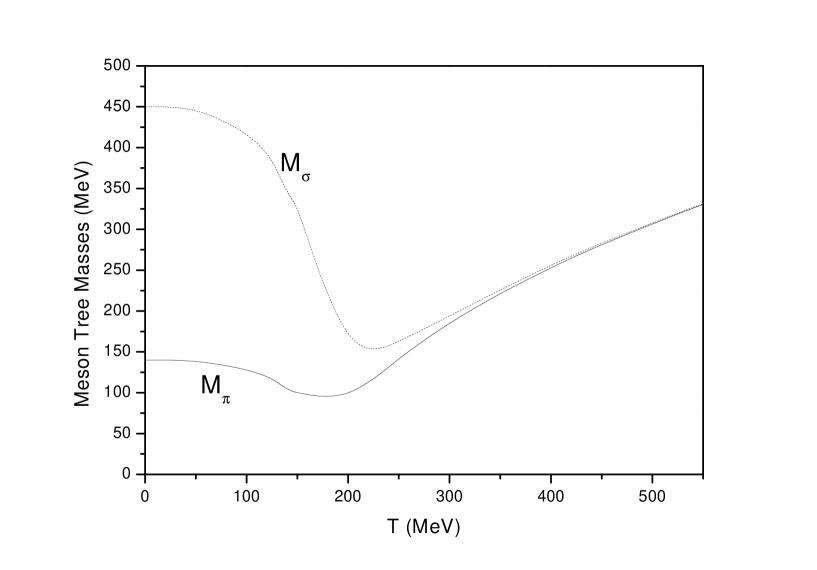
Let us analyze the finite temperature behavior of the tree-level meson masses (19) and (20) as functions of the thermal expectation value of the sigma field, ν(T)𝜈𝑇\nu(T). Since ν2(T)superscript𝜈2𝑇\nu^{2}(T) decreases as T𝑇T increases and m2<0superscript𝑚20m^{2}<0, the particle masses becomes tachyonic. Another problem which arises is the fact that Goldstone’s theorem is not satisfied in the ordered phase (when c=0𝑐0c=0), i.e., replacing (44) on (19), we obtain a non zero pion mass given by mπ2=λ2(1+2g23λ)T2superscriptsubscript𝑚𝜋2𝜆212superscript𝑔23𝜆superscript𝑇2m_{\pi}^{2}=-\frac{\lambda}{2}(1+\frac{2g^{2}}{3\lambda})T^{2}. This pathological behavior is due to the fact that in our approximation we have neglect the interaction action SIsubscript𝑆𝐼S_{I} in the thermodynamical potential (29). The result is that the mean field approximation can be trusted only in the approximate prediction of a phase transition at Tcsubscript𝑇𝑐T_{c} given by (45). It is incorrect in what concern the description of the finite temperature behavior of the meson and fermion masses. So it is necessary to include all one-loop corrections from all 1PI diagrams present in SIsubscript𝑆𝐼S_{I} to the masses.

Following the program of [13] we expand the partition function in powers of the interaction, in order to get the one-loop self-energy corrections.

lnZI=ln(1+n=11n![dϕ]eS0SIn[dϕ]eS0)subscript𝑍𝐼1superscriptsubscript𝑛11𝑛delimited-[]𝑑italic-ϕsuperscript𝑒subscript𝑆0superscriptsubscript𝑆𝐼𝑛delimited-[]𝑑italic-ϕsuperscript𝑒subscript𝑆0\ln Z_{I}=\ln(1+\sum_{n=1}^{\infty}\frac{1}{n!}\frac{\int[d\phi]e^{S_{0}}S_{I}^{n}}{[d\phi]e^{S_{0}}}) (46)

The one-loop 1PI graphs come from lnZ1+lnZ2subscript𝑍1subscript𝑍2\ln Z_{1}+\ln Z_{2}, which are given by

lnZ1=[dϕ]eS0SI[dϕ]eS0subscript𝑍1delimited-[]𝑑italic-ϕsuperscript𝑒subscript𝑆0subscript𝑆𝐼delimited-[]𝑑italic-ϕsuperscript𝑒subscript𝑆0\ln Z_{1}=\frac{\int[d\phi]e^{S_{0}}S_{I}}{[d\phi]e^{S_{0}}} (47)
lnZ2=12([dϕ]eS0SI[dϕ]eS0)2+12[dϕ]eS0SI2[dϕ]eS0subscript𝑍212superscriptdelimited-[]𝑑italic-ϕsuperscript𝑒subscript𝑆0subscript𝑆𝐼delimited-[]𝑑italic-ϕsuperscript𝑒subscript𝑆0212delimited-[]𝑑italic-ϕsuperscript𝑒subscript𝑆0superscriptsubscript𝑆𝐼2delimited-[]𝑑italic-ϕsuperscript𝑒subscript𝑆0\ln Z_{2}=-\frac{1}{2}(\frac{\int[d\phi]e^{S_{0}}S_{I}}{[d\phi]e^{S_{0}}})^{2}+\frac{1}{2}\frac{\int[d\phi]e^{S_{0}}S_{I}^{2}}{[d\phi]e^{S_{0}}} (48)

where the disconnected diagrams cancel in lnZ2𝑙𝑛subscript𝑍2lnZ_{2} and the diagrams which gives rise to tadpoles in the self-energy are not to be included, since their effect is already considered in the mean field equation. The terms which “survive” come from:

lnZI2loop=λ4[dϕ]eS0𝑑τd3x(π2+σ2)2[dϕ]eSo+superscriptsubscript𝑍𝐼2𝑙𝑜𝑜𝑝limit-from𝜆4delimited-[]𝑑italic-ϕsuperscript𝑒subscript𝑆0differential-d𝜏superscript𝑑3𝑥superscriptsuperscript𝜋2superscript𝜎22delimited-[]𝑑italic-ϕsuperscript𝑒subscript𝑆𝑜\displaystyle\ln Z_{I}^{2-loop}=-\frac{\lambda}{4}\frac{\int[d\phi]e^{S_{0}}\int d\tau\int d^{3}x(\pi^{2}+\sigma^{2})^{2}}{\int[d\phi]e^{S_{o}}}+ (49)
120β𝑑τ1𝑑τ2d3x1d3x2[dϕ]eS0{λ2ν2[(σπ2)2+(σ3)2]+g2[(ψ¯σψ)2+(ψ¯iγ5πτψ)2]}[dϕ]eS012superscriptsubscript0𝛽differential-dsubscript𝜏1differential-dsubscript𝜏2superscript𝑑3subscript𝑥1superscript𝑑3subscript𝑥2delimited-[]𝑑italic-ϕsuperscript𝑒subscript𝑆0superscript𝜆2superscript𝜈2delimited-[]superscript𝜎superscript𝜋22superscriptsuperscript𝜎32superscript𝑔2delimited-[]superscript¯𝜓𝜎𝜓2superscript¯𝜓𝑖superscript𝛾5𝜋𝜏𝜓2delimited-[]𝑑italic-ϕsuperscript𝑒subscript𝑆0\displaystyle\frac{1}{2}\int_{0}^{\beta}d\tau_{1}d\tau_{2}\int d^{3}x_{1}d^{3}x_{2}\frac{\int[d\phi]e^{S_{0}}\left\{{\lambda^{2}\nu^{2}}[(\sigma\pi^{2})^{2}+(\sigma^{3})^{2}]+{g^{2}}[(\overline{\psi}\sigma\psi)^{2}+(\overline{\psi}i\gamma^{5}{\vec{\pi}}\cdot{\vec{\tau}}\psi)^{2}]\right\}}{\int[d\phi]e^{S_{0}}} (50)

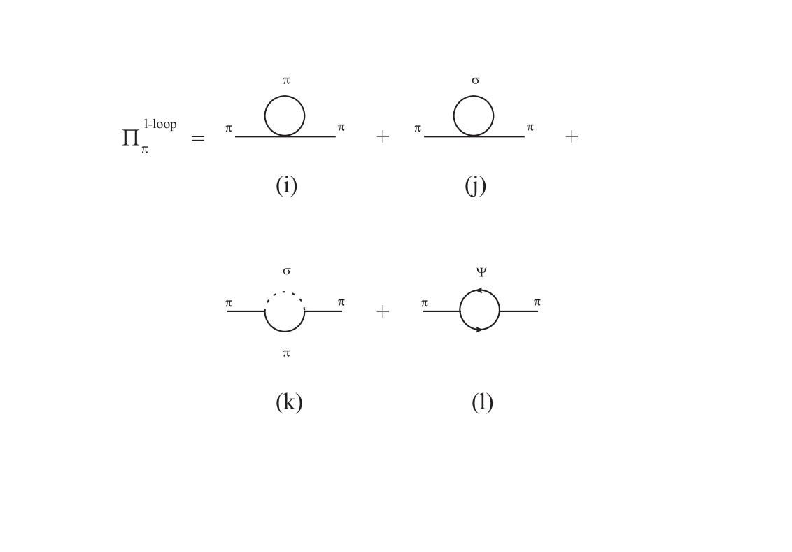
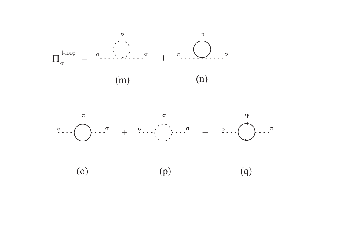
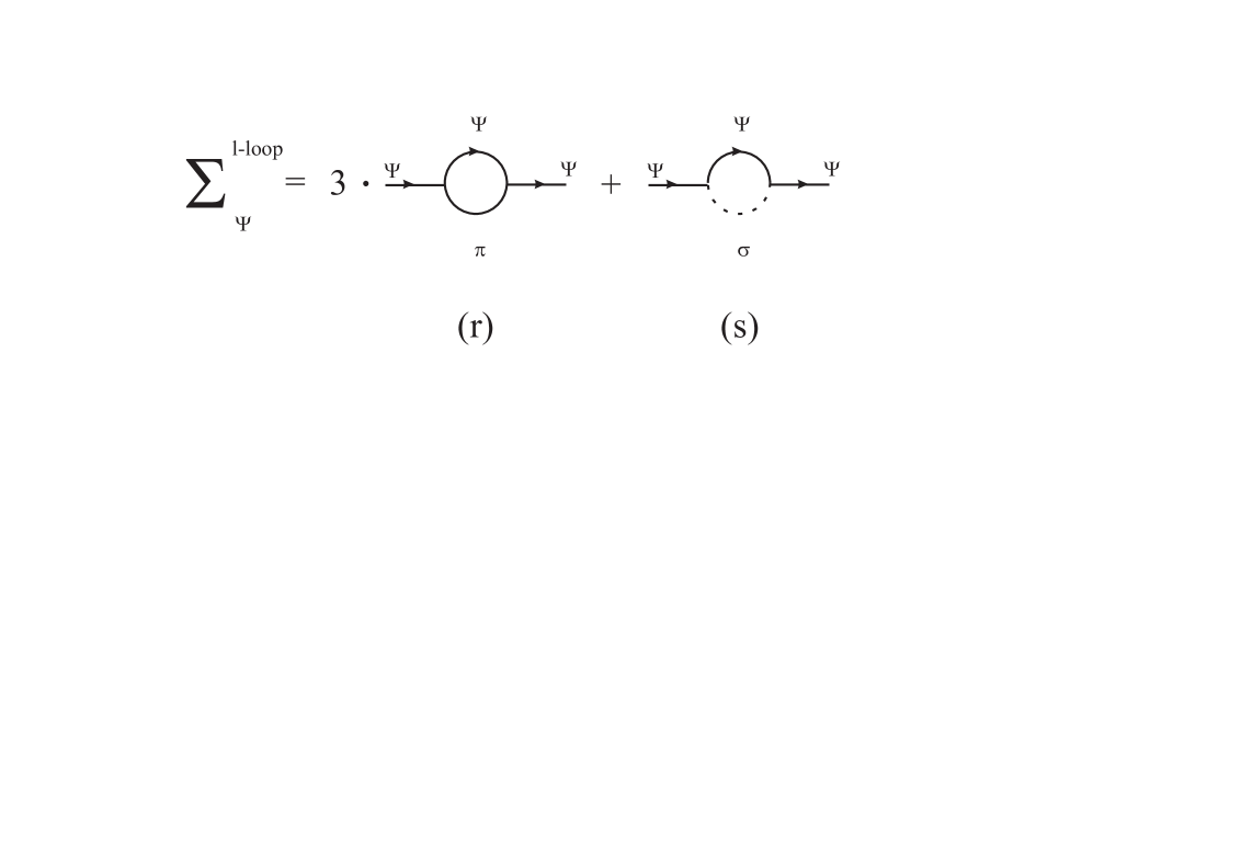
The 1PI graphs from this expression can be represented diagrammatically as shown in Fig.1.

The self-energy for bosons and fermions are defined, respectively by

𝐃(ωn,𝐤)σ,π1=𝐃0σ,π(ωn,𝐤)1+Πσ,π(ωn,𝐤)𝐃superscriptsubscriptsubscript𝜔𝑛𝐤𝜎𝜋1subscript𝐃0𝜎𝜋superscriptsubscript𝜔𝑛𝐤1subscriptΠ𝜎𝜋subscript𝜔𝑛𝐤{\bf D}(\omega_{n},{\bf k})_{\sigma,\pi}^{-1}={\bf D}_{0\sigma,\pi}(\omega_{n},{\bf k})^{-1}+\Pi_{\sigma,\pi}(\omega_{n},{\bf k}) (51)
𝒟(ωn,𝐤)1=𝒟0(ωn,𝐤)1+Σ(ωn,𝐤)𝒟superscriptsubscript𝜔𝑛𝐤1subscript𝒟0superscriptsubscript𝜔𝑛𝐤1Σsubscript𝜔𝑛𝐤{\cal D}(\omega_{n},{\bf k})^{-1}={\cal D}_{0}(\omega_{n},{\bf k})^{-1}+\Sigma(\omega_{n},{\bf k}) (52)

where 𝐃0σ,π(ωn,𝐩)subscript𝐃0𝜎𝜋subscript𝜔𝑛𝐩{\bf D}_{0\sigma,\pi}(\omega_{n},{\bf p}) and 𝒟0(ωn,𝐩)subscript𝒟0subscript𝜔𝑛𝐩{\cal D}_{0}(\omega_{n},{\bf p}) are the tree-level boson and fermion propagators, expressed respectively as

𝐃0σ,π(ωn,𝐤)1=ωn2+𝐤2+mσ,π2subscript𝐃0𝜎𝜋superscriptsubscript𝜔𝑛𝐤1superscriptsubscript𝜔𝑛2superscript𝐤2superscriptsubscript𝑚𝜎𝜋2{\bf D}_{0\sigma,\pi}(\omega_{n},{\bf k})^{-1}=\omega_{n}^{2}+{\bf k}^{2}+m_{\sigma,\pi}^{2} (53)
𝒟0(ωn,𝐤)1=γμkμmψsubscript𝒟0superscriptsubscript𝜔𝑛𝐤1subscript𝛾𝜇superscript𝑘𝜇subscript𝑚𝜓{\cal D}_{0}(\omega_{n},{\bf k})^{-1}=\gamma_{\mu}k^{\mu}-m_{\psi} (54)

Here, ωnsubscript𝜔𝑛\omega_{n} are the Matsubara frequencies, defined as ωn=2nπTsubscript𝜔𝑛2𝑛𝜋𝑇\omega_{n}=2n\pi T for bosons and ωn=(2n+1)πTωnfsubscript𝜔𝑛2𝑛1𝜋𝑇subscript𝜔𝑛𝑓\omega_{n}=(2n+1)\pi T\equiv\omega_{nf} for fermions.

To one-loop order the self-energy expressions are given[13] by

Πσ,π=2(δlnZI2loopδ𝐃0σ,π)1PIsubscriptΠ𝜎𝜋2subscript𝛿superscriptsubscript𝑍𝐼2𝑙𝑜𝑜𝑝𝛿subscript𝐃0𝜎𝜋1𝑃𝐼\Pi_{\sigma,\pi}=-2(\frac{\delta\ln Z_{I}^{2-loop}}{\delta{{\bf D}}_{0\sigma,\pi}})_{1PI} (55)
Σ=(δlnZI2loopδ𝒟0ψ)1PIΣsubscript𝛿superscriptsubscript𝑍𝐼2𝑙𝑜𝑜𝑝𝛿subscript𝒟0𝜓1𝑃𝐼\Sigma=(\frac{\delta\ln Z_{I}^{2-loop}}{\delta{\cal D}_{0\psi}})_{1PI} (56)

The self-energy graphs to each particle can be pictorially represented as by cutting one of the corresponding loops in the diagrams representing (lnZI2loop)1PIsubscriptsuperscriptsubscript𝑍𝐼2𝑙𝑜𝑜𝑝1𝑃𝐼(\ln Z_{I}^{2-loop})_{1PI}. After the integration in x𝑥x, τ𝜏\tau and in the fields in (lnZI2loop)1PIsubscriptsuperscriptsubscript𝑍𝐼2𝑙𝑜𝑜𝑝1𝑃𝐼(\ln Z_{I}^{2-loop})_{1PI} and the differentiations above, we obtain the following expressions for the self-energies at one loop order

Ππ(k0,𝐤)=i=14Ππi=λ5Tnd3p(2π)3𝐃0π(ωn,𝐩)+λTnd3p(2π)3𝐃0σ(ωn,𝐩)+subscriptΠ𝜋subscript𝑘0𝐤superscriptsubscript𝑖14subscriptΠ𝜋𝑖𝜆5𝑇subscript𝑛superscript𝑑3𝑝superscript2𝜋3subscript𝐃0𝜋subscript𝜔𝑛𝐩limit-from𝜆𝑇subscript𝑛superscript𝑑3𝑝superscript2𝜋3subscript𝐃0𝜎subscript𝜔𝑛𝐩\displaystyle\Pi_{\pi}(k_{0},{\bf k})=\sum_{i=1}^{4}\Pi_{\pi i}=\lambda 5T\sum_{n}\int\frac{d^{3}p}{(2\pi)^{3}}{\bf D}_{0\pi}(\omega_{n},{\bf p})+\lambda T\sum_{n}\int\frac{d^{3}p}{(2\pi)^{3}}{\bf D}_{0\sigma}(\omega_{n},{\bf p})+ (57)
4λ2ν2Tnd3p(2π)3𝐃0σ(ωn+l,𝐩+𝐤)𝐃0π(ωn,𝐩)+g2Tnd3p(2π)3Tr[γ5𝒟0ψ(ωn+l,𝐩+𝐤)γ5𝒟0ψ(ωn,𝐩)]4superscript𝜆2superscript𝜈2𝑇subscript𝑛superscript𝑑3𝑝superscript2𝜋3subscript𝐃0𝜎subscript𝜔𝑛𝑙𝐩𝐤subscript𝐃0𝜋subscript𝜔𝑛𝐩superscript𝑔2𝑇subscript𝑛superscript𝑑3𝑝superscript2𝜋3Trdelimited-[]superscript𝛾5subscript𝒟0𝜓subscript𝜔𝑛𝑙𝐩𝐤superscript𝛾5subscript𝒟0𝜓subscript𝜔𝑛𝐩\displaystyle-4\lambda^{2}\nu^{2}T\sum_{n}\int\frac{d^{3}p}{(2\pi)^{3}}{\bf D}_{0\sigma}(\omega_{n+l},{\bf p}+{\bf k}){\bf D}_{0\pi}(\omega_{n},{\bf p})+g^{2}T\sum_{n}\int\frac{d^{3}p}{(2\pi)^{3}}{\rm Tr}[\gamma^{5}{\cal D}_{0\psi}(\omega_{n+l},{\bf p}+{\bf k})\gamma^{5}{\cal D}_{0\psi}(\omega_{n},{\bf p})] (58)
Πσ(k0,𝐤)=i=15Πσi=3λTnd3p(2π)3𝐃0σ(ωn,𝐩)+3λTnd3p(2π)3𝐃0π(ωn,𝐩)+subscriptΠ𝜎subscript𝑘0𝐤superscriptsubscript𝑖15subscriptΠ𝜎𝑖3𝜆𝑇subscript𝑛superscript𝑑3𝑝superscript2𝜋3subscript𝐃0𝜎subscript𝜔𝑛𝐩limit-from3𝜆𝑇subscript𝑛superscript𝑑3𝑝superscript2𝜋3subscript𝐃0𝜋subscript𝜔𝑛𝐩\displaystyle\Pi_{\sigma}(k_{0},{\bf k})=\sum_{i=1}^{5}\Pi_{\sigma i}=3\lambda T\sum_{n}\int\frac{d^{3}p}{(2\pi)^{3}}{\bf D}_{0\sigma}(\omega_{n},{\bf p})+3\lambda T\sum_{n}\int\frac{d^{3}p}{(2\pi)^{3}}{\bf D}_{0\pi}(\omega_{n},{\bf p})+ (59)
6λ2ν2Tnd3p(2π)3𝐃0π(ωn+l,𝐩+𝐤)𝐃0π(ωn,𝐩)18λ2ν2Tnd3p(2π)3𝐃0σ(ωn+l,𝐩+𝐤)𝐃0σ(ωn,𝐩)+6superscript𝜆2superscript𝜈2𝑇subscript𝑛superscript𝑑3𝑝superscript2𝜋3subscript𝐃0𝜋subscript𝜔𝑛𝑙𝐩𝐤subscript𝐃0𝜋subscript𝜔𝑛𝐩limit-from18superscript𝜆2superscript𝜈2𝑇subscript𝑛superscript𝑑3𝑝superscript2𝜋3subscript𝐃0𝜎subscript𝜔𝑛𝑙𝐩𝐤subscript𝐃0𝜎subscript𝜔𝑛𝐩\displaystyle-6\lambda^{2}\nu^{2}T\sum_{n}\int\frac{d^{3}p}{(2\pi)^{3}}{\bf D}_{0\pi}(\omega_{n+l},{\bf p}+{\bf k}){\bf D}_{0\pi}(\omega_{n},{\bf p})-18\lambda^{2}\nu^{2}T\sum_{n}\int\frac{d^{3}p}{(2\pi)^{3}}{\bf D}_{0\sigma}(\omega_{n+l},{\bf p}+{\bf k}){\bf D}_{0\sigma}(\omega_{n},{\bf p})+ (60)
g2Tnd3p(2π)3Tr[𝒟0ψ(ωn+l,𝐩+𝐤)𝒟0ψ(ωn,𝐩)]superscript𝑔2𝑇subscript𝑛superscript𝑑3𝑝superscript2𝜋3Trdelimited-[]subscript𝒟0𝜓subscript𝜔𝑛𝑙𝐩𝐤subscript𝒟0𝜓subscript𝜔𝑛𝐩\displaystyle g^{2}T\sum_{n}\int\frac{d^{3}p}{(2\pi)^{3}}{\rm Tr}[{\cal D}_{0\psi}(\omega_{n+l},{\bf p}+{\bf k}){\cal D}_{0\psi}(\omega_{n},{\bf p})] (61)
Σ(k0,𝐤)=i=12Σi=g2Tnd3p(2π)3𝐃0σ(ωn+l,𝐩+𝐤)𝒟0ψ(ωn,𝐩)+Σsubscript𝑘0𝐤superscriptsubscript𝑖12subscriptΣ𝑖limit-fromsuperscript𝑔2𝑇subscript𝑛superscript𝑑3𝑝superscript2𝜋3subscript𝐃0𝜎subscript𝜔𝑛𝑙𝐩𝐤subscript𝒟0𝜓subscript𝜔𝑛𝐩\displaystyle\Sigma(k_{0},{\bf k})=\sum_{i=1}^{2}\Sigma_{i}=-g^{2}T\sum_{n}\int\frac{d^{3}p}{(2\pi)^{3}}{\bf D}_{0\sigma}(\omega_{n+l},{\bf p}+{\bf k}){\cal D}_{0\psi}(\omega_{n},{\bf p})+ (62)
3g2Tnd3p(2π)3𝐃0π(ωn+l,𝐩+𝐤)𝒟0ψ(ωn,𝐩)3superscript𝑔2𝑇subscript𝑛superscript𝑑3𝑝superscript2𝜋3subscript𝐃0𝜋subscript𝜔𝑛𝑙𝐩𝐤subscript𝒟0𝜓subscript𝜔𝑛𝐩\displaystyle-3g^{2}T\sum_{n}\int\frac{d^{3}p}{(2\pi)^{3}}{\bf D}_{0\pi}(\omega_{n+l},{\bf p}+{\bf k}){\cal D}_{0\psi}(\omega_{n},{\bf p}) (63)

The diagrams representing the pion, sigma and nucleon one-loop self-energies are drawn in figures 2,3 and 4.

We note here that we could get the same results for the self-energies directly applying Feynman rules to construct the diagrams with the appropriate substitutions: the δ𝛿\delta-function at each vertex is replaced with a Kronecker delta which imposes conservation of the discrete energy (k0=iωnsubscript𝑘0𝑖subscript𝜔𝑛k_{0}=i\omega_{n}), and round each loop of a thermal graph with d4k(2π)4iβnd3k(2π)3superscript𝑑4𝑘superscript2𝜋4𝑖𝛽subscript𝑛superscript𝑑3𝑘superscript2𝜋3\int\frac{d^{4}k}{(2\pi)^{4}}\to\frac{i}{\beta}\sum_{n}\int\frac{d^{3}k}{(2\pi)^{3}},which are the finite-temperature Feynman rules[13, 23]. When the summation over n𝑛n is performed, each graph of the self-energies is separated into two parts, namely a temperature independent part(at this stage), which is divergent, and a temperature dependent part containing the Bose-Einstein distribution in the case of bosons or the Fermi-Dirac distribution for fermions.

We will adopt the definition of mass at finite temperature as the real part of the pole of the corrected propagator at zero momentum (𝐤=0)𝐤0({\bf k}=0). Thus, from eqs. (51) and (52) we have

𝐃π(ωn,|𝐤|=0)1=ωn2+mπ2+Ππ(ωn,|𝐤|=0)=0subscript𝐃𝜋superscriptsubscript𝜔𝑛𝐤01superscriptsubscript𝜔𝑛2superscriptsubscript𝑚𝜋2subscriptΠ𝜋subscript𝜔𝑛𝐤00absent\displaystyle{\bf D}_{\pi}(\omega_{n},\left|{\bf k}\right|=0)^{-1}=\omega_{n}^{2}+m_{\pi}^{2}+\Pi_{\pi}(\omega_{n},\left|{\bf k}\right|=0)=0\to (64)
k0,π2+mπ2+Ππ(T,k0,π,|𝐤|=0)=0superscriptsubscript𝑘0𝜋2superscriptsubscript𝑚𝜋2subscriptΠ𝜋𝑇subscript𝑘0𝜋𝐤00\displaystyle-k_{0,\pi}^{2}+m_{\pi}^{2}+\Pi_{\pi}(T,k_{0,\pi},\left|{\bf k}\right|=0)=0 (65)
𝐃σ(ωn,|𝐤|=0)1=ωn2+mσ2+Πσ(ωn,|𝐤|=0)=0subscript𝐃𝜎superscriptsubscript𝜔𝑛𝐤01superscriptsubscript𝜔𝑛2superscriptsubscript𝑚𝜎2subscriptΠ𝜎subscript𝜔𝑛𝐤00absent\displaystyle{\bf D}_{\sigma}(\omega_{n},\left|{\bf k}\right|=0)^{-1}=\omega_{n}^{2}+m_{\sigma}^{2}+\Pi_{\sigma}(\omega_{n},\left|{\bf k}\right|=0)=0\to (66)
k0,σ2+mσ2+Πσ(T,k0,σ,|𝐤|=0)=0superscriptsubscript𝑘0𝜎2superscriptsubscript𝑚𝜎2subscriptΠ𝜎𝑇subscript𝑘0𝜎𝐤00\displaystyle-k_{0,\sigma}^{2}+m_{\sigma}^{2}+\Pi_{\sigma}(T,k_{0,\sigma},\left|{\bf k}\right|=0)=0 (67)
𝒟ψ(ωnf,|𝐤|=0)1=γμkμmψ+Σs+γμΣμ=0subscript𝒟𝜓superscriptsubscript𝜔𝑛𝑓𝐤01superscript𝛾𝜇subscript𝑘𝜇subscript𝑚𝜓subscriptΣ𝑠superscript𝛾𝜇subscriptΣ𝜇0absent\displaystyle{\cal D}_{\psi}(\omega_{n}f,\left|{\bf k}\right|=0)^{-1}=\gamma^{\mu}k_{\mu}-m_{\psi}+\Sigma_{s}+\gamma^{\mu}\Sigma_{\mu}=0\to (68)
k0,ψ+Σ0(T,k0,ψ,|𝐤|=0)+Σs(T,k0,ψ|𝐤|=0)mψ=0,subscript𝑘0𝜓subscriptΣ0𝑇subscript𝑘0𝜓𝐤0subscriptΣ𝑠𝑇subscript𝑘0𝜓𝐤0subscript𝑚𝜓0\displaystyle k_{0,\psi}+\Sigma_{0}(T,k_{0,\psi},\left|{\bf k}\right|=0)+\Sigma_{s}(T,k_{0,\psi}\left|{\bf k}\right|=0)-m_{\psi}=0, (69)

where the arrow indicates an analytical continuation from discrete to continuous energies in Minkowski space. Hence the physical masses are the values of the k0;π,σ,ψsubscript𝑘0𝜋𝜎𝜓k_{0;\pi,\sigma,\psi} which are the zeros of the functions (64), (66) and (68) above, i.e., the location of the poles in the limit 𝐤=0𝐤0{\bf k}=0. The full self-energy expressions ΠπsubscriptΠ𝜋\Pi_{\pi}, ΠσsubscriptΠ𝜎\Pi_{\sigma}, Σ0subscriptΣ0\Sigma_{0} and ΣssubscriptΣ𝑠\Sigma_{s} are shown explicitly in appendix B. The renormalization of the self-energy is studied in section VI. Through out this paper, we will use dimensional regularization, but omitting, for notational simplicity the factor μ2ϵsuperscript𝜇2italic-ϵ\mu^{2\epsilon} which multiplies λ𝜆\lambda. Since our calculations does not require traces involving an odd number of γ5superscript𝛾5\gamma^{5} matrices, we use the definition of γ5superscript𝛾5\gamma^{5} as in[24, 25].

Since these expressions are self-consistent they have to be solved numerically. For each fixed temperature one finds a value of M𝑀M which satisfies the equations above. On the other hand, if one is interested only in the meson sector of the linear sigma model, the integrals in the self-energies could be evaluated exactly in the high temperature limit and at low frequency where the boson diagrams involving three-point vertices which are proportional to λ2ν2superscript𝜆2superscript𝜈2\lambda^{2}\nu^{2} may be neglected. This is not consistent if one wants to study the behavior of the condensate ν𝜈\nu and the particle masses in all ranges of temperatures. It is important to note that when c=0𝑐0c=0 the three-point vertex boson diagrams are significant in the region Ti(0)<T<Tf(ν(T))annotatedsubscript𝑇𝑖similar-toabsent0𝑇annotatedsubscript𝑇𝑓similar-toabsent𝜈𝑇T_{i}(\sim 0)<T<T_{f}(\sim\nu(T)) and when c0𝑐0c\neq 0, ν(T)0𝜈𝑇0\nu(T)\neq 0 for any finite value of T.

B The second necessity: The resummation

The expressions for the self-energies appearing in eq. (64), (66) and (68) are functions of ωπ,σ,ψsubscript𝜔𝜋𝜎𝜓\omega_{\pi,\sigma,\psi} which are expressed in terms of the mean-field masses. As we discussed, the meson masses become negative as the temperature increases. Thus, in the computation of the one-loop corrections, the masses running in the loops become tachyonic. A proper resummation of higher order loops is naturally necessary [6]. Various resummation methods have been proposed in a tentative of curing the problem of the breaking down of the perturbative expansion at high temperature. In effective models, when a phase transition occurs, one can find tachyonic masses even below Tcsubscript𝑇𝑐T_{c}. The O(N) linear σ𝜎\sigma model which is one of the laboratory effective models employed to study QCD has been investigated by different authors using different techniques. One of these methods is the CJT formalism [26] which provides for a consistent loop expansion of the effective potential in terms of the full propagator. The CJT formalism elegantly provides for a gap equation from stationarity conditions for the daisy and super-daisy effective potential. However some authors use this non-perturbative approach with an ansatz for the full (corrected) propagator in which the thermal corrections are momentum independent. These corrections are the finite piece of the divergent integral (which is temperature dependent through the gap equation for M𝑀M) plus the finite explicit temperature dependent piece. This is the Hartree approximation, and means resuming only the “bubble diagrams” that are dominant at high temperatures. Another non-perturbative approach widely found in the literature is the large-N𝑁N approximation. The N𝑁N\to\infty limit facilitates the calculations, but can lead to inaccuracies [27, 19]. One must be careful in taking the large-N𝑁N limit since its truncation depends on the problem to be studied and the relevant value of N𝑁N [27]. In this case the three-point vertex diagrams are omitted which in principle makes sense only in the N𝑁N\to\infty limit since these sunset diagrams are of order 1/N1𝑁1/N. In these two kinds of treatment one can not study the bosons interacting with fermions (with the interactions of the linear sigma model) since the self-energy diagrams are momentum dependent which invalidates the ansatz cited above. It is worth to remember that the Hartree approximation does not satisfies the Goldstone theorem[19, 28]. This fact may be attributed to the non inclusion of these diagrams. Although the finite temperature mass in these approaches is the pole of the corrected propagator, it is not the true mass, since their Ππ,σsubscriptΠ𝜋𝜎\Pi_{\pi,\sigma} are not the true one-loop self-energy functions (see discussion below). The corrections included only shift the masses. Once we are interested in the study of the masses behavior also in the range 0<T<Tc0𝑇subscript𝑇𝑐0<T<T_{c} (if c=0𝑐0c=0) the three-particle vertex diagrams will not be neglected. The inclusion of these diagrams brings an additional complication since the self-energy now depends on the momentum.

C A non-perturbative resummation method: The MSCR

Let us now introduce our procedure which resumms higher loop diagrams in the mean-field (tree-level) propagators. The method consist in recalculating the self-energy, in steps, using in each step the masses obtained in the previous one such that Mn2=(An+1)Mn12+Π(Mn1)superscriptsubscript𝑀𝑛2subscript𝐴𝑛1superscriptsubscript𝑀𝑛12Πsubscript𝑀𝑛1M_{n}^{2}=(A_{n}+1)M_{n-1}^{2}+\Pi(M_{n-1}), where n𝑛n is the order of the non-perturbative correction and Ansubscript𝐴𝑛A_{n} is the coefficient of the appropriate counterterm. With this procedure it is easier to identify and absorb the divergent parts of the self-energy in order to have finite gap-equations. The goal is to make renormalization possible since the masses which multiply the divergences are necessarily the same as in counterterms.

Application of MSCR

Here we apply the MSCR in the study of the chiral fermion meson model at finite temperature. The analysis of the problem has to be done carefully which will be divided into three regions.

Region I: The low temperature region

The first region is for 0T<T0𝑇superscript𝑇0\leq T<T^{*}, where Tsuperscript𝑇T^{*} is the temperature where ν(T)=fπ𝜈superscript𝑇subscript𝑓𝜋\nu(T^{*})=f_{\pi}. This implies that mπ2=0superscriptsubscript𝑚𝜋20m_{\pi}^{2}=0 and consequently the appearance of infrared divergences in the self-energy. So, in this region

Step 1:

Start with the mean-field effective Lagrangian where the condensate and the masses are given by:

[F(ωπ,σ,ψ(mπ,σ,ψ;0),T)+G(ωπ,σ,ψ(mπ,σ,ψ;0))λ(fπ2ν2)]νc=0,delimited-[]𝐹subscript𝜔𝜋𝜎𝜓subscript𝑚𝜋𝜎𝜓0𝑇𝐺subscript𝜔𝜋𝜎𝜓subscript𝑚𝜋𝜎𝜓0𝜆superscriptsubscript𝑓𝜋2superscript𝜈2𝜈𝑐0\left[F\left(\omega_{\pi,\sigma,\psi}(m_{\pi,\sigma,\psi;0}),T\right)+G\left(\omega_{\pi,\sigma,\psi}(m_{\pi,\sigma,\psi;0})\right)-\lambda(f_{\pi}^{2}-\nu^{2})\right]\nu-c=0, (70)
Mπ,02=mπ2=m2+λν2,superscriptsubscript𝑀𝜋02superscriptsubscript𝑚𝜋2superscript𝑚2𝜆superscript𝜈2M_{\pi,0}^{2}=m_{\pi}^{2}=m^{2}+\lambda\nu^{2}, (71)
Mσ,02=mσ2=m2+3λν2,superscriptsubscript𝑀𝜎02superscriptsubscript𝑚𝜎2superscript𝑚23𝜆superscript𝜈2M_{\sigma,0}^{2}=m_{\sigma}^{2}=m^{2}+3\lambda\nu^{2}, (72)
Mψ,0=mψ=gν.subscript𝑀𝜓0subscript𝑚𝜓𝑔𝜈M_{\psi,0}=m_{\psi}=g\nu. (73)

Step 2:

Evaluate the one-loop self-energy corrections to these masses from the equations presented in appendix B and define the condensate and the first order corrected masses as

[F(ωπ,σ,ψ(Mπ,σ,ψ,0),T)+G(ωπ,σ,ψ(Mπ,σ,ψ,0))λ(fπ2ν2)]νc=0,delimited-[]𝐹subscript𝜔𝜋𝜎𝜓subscript𝑀𝜋𝜎𝜓0𝑇𝐺subscript𝜔𝜋𝜎𝜓subscript𝑀𝜋𝜎𝜓0𝜆superscriptsubscript𝑓𝜋2superscript𝜈2𝜈𝑐0\left[F\left(\omega_{\pi,\sigma,\psi}(M_{\pi,\sigma,\psi,0}),T\right)+G\left(\omega_{\pi,\sigma,\psi}(M_{\pi,\sigma,\psi,0})\right)-\lambda(f_{\pi}^{2}-\nu^{2})\right]\nu-c=0, (74)
Mπ,12=Mπ,02+Ππ(Mπ,02,Mσ,02,Mψ,0)=superscriptsubscript𝑀𝜋12superscriptsubscript𝑀𝜋02subscriptΠ𝜋superscriptsubscript𝑀𝜋02superscriptsubscript𝑀𝜎02subscript𝑀𝜓0absent\displaystyle M_{\pi,1}^{2}=M_{\pi,0}^{2}+\Pi_{\pi}(M_{\pi,0}^{2},M_{\sigma,0}^{2},M_{\psi,0})= (75)
(A1+E1+1)m2+(A¯1+E1+1)λν2+Ππ(Mπ,02,Mσ,02,Mψ,0)=subscript𝐴1subscript𝐸11superscript𝑚2subscript¯𝐴1subscript𝐸11𝜆superscript𝜈2subscriptΠ𝜋superscriptsubscript𝑀𝜋02superscriptsubscript𝑀𝜎02subscript𝑀𝜓0absent\displaystyle(A_{1}+E_{1}+1)m^{2}+(\overline{A}_{1}+E_{1}+1)\lambda\nu^{2}+\Pi_{\pi}(M_{\pi,0}^{2},M_{\sigma,0}^{2},M_{\psi,0})= (76)
m2+λν2+ΠπRen(Mπ,02,Mσ,02,Mψ,0),superscript𝑚2𝜆superscript𝜈2superscriptsubscriptΠ𝜋𝑅𝑒𝑛superscriptsubscript𝑀𝜋02superscriptsubscript𝑀𝜎02subscript𝑀𝜓0\displaystyle m^{2}+\lambda\nu^{2}+\Pi_{\pi}^{Ren}(M_{\pi,0}^{2},M_{\sigma,0}^{2},M_{\psi,0}), (77)
Mσ,12=Mσ,02+Πσ(Mπ,02,Mσ,02,Mψ,0)=superscriptsubscript𝑀𝜎12superscriptsubscript𝑀𝜎02subscriptΠ𝜎superscriptsubscript𝑀𝜋02superscriptsubscript𝑀𝜎02subscript𝑀𝜓0absent\displaystyle M_{\sigma,1}^{2}=M_{\sigma,0}^{2}+\Pi_{\sigma}(M_{\pi,0}^{2},M_{\sigma,0}^{2},M_{\psi,0})= (78)
(B1+F1+1)m2+(F1+1)λν2+(B¯1+1)2λν2+Πσ(Mπ,02,Mσ,02,Mψ,0)=subscript𝐵1subscript𝐹11superscript𝑚2subscript𝐹11𝜆superscript𝜈2subscript¯𝐵112𝜆superscript𝜈2subscriptΠ𝜎superscriptsubscript𝑀𝜋02superscriptsubscript𝑀𝜎02subscript𝑀𝜓0absent\displaystyle(B_{1}+F_{1}+1)m^{2}+(F_{1}+1)\lambda\nu^{2}+(\overline{B}_{1}+1)2\lambda\nu^{2}+\Pi_{\sigma}(M_{\pi,0}^{2},M_{\sigma,0}^{2},M_{\psi,0})= (79)
m2+3λν2+ΠσRen(Mπ,02,Mσ,02,Mψ,0),superscript𝑚23𝜆superscript𝜈2superscriptsubscriptΠ𝜎𝑅𝑒𝑛superscriptsubscript𝑀𝜋02superscriptsubscript𝑀𝜎02subscript𝑀𝜓0\displaystyle m^{2}+3\lambda\nu^{2}+\Pi_{\sigma}^{Ren}(M_{\pi,0}^{2},M_{\sigma,0}^{2},M_{\psi,0}), (80)
Mψ,1=Mψ,0Σ(Mπ,02,Mσ,02,Mψ,0)=subscript𝑀𝜓1subscript𝑀𝜓0Σsuperscriptsubscript𝑀𝜋02superscriptsubscript𝑀𝜎02subscript𝑀𝜓0absent\displaystyle M_{\psi,1}=M_{\psi,0}-\Sigma(M_{\pi,0}^{2},M_{\sigma,0}^{2},M_{\psi,0})= (81)
(C1+1)gνΣ(Mπ,02,Mσ,02,Mψ,0)=subscript𝐶11𝑔𝜈Σsuperscriptsubscript𝑀𝜋02superscriptsubscript𝑀𝜎02subscript𝑀𝜓0absent\displaystyle(C_{1}+1)g\nu-\Sigma(M_{\pi,0}^{2},M_{\sigma,0}^{2},M_{\psi,0})= (82)
gνΣRen(Mπ,02,Mσ,02,Mψ,0).𝑔𝜈superscriptΣ𝑅𝑒𝑛superscriptsubscript𝑀𝜋02superscriptsubscript𝑀𝜎02subscript𝑀𝜓0\displaystyle g\nu-\Sigma^{Ren}(M_{\pi,0}^{2},M_{\sigma,0}^{2},M_{\psi,0}). (83)

where Ππ,σ=Ππ,σ(k0,π,σ=Mπ,σ;𝐤=0)0+Ππ,σ(T;k0,π,σ=0;𝐤=0)β\Pi_{\pi,\sigma}=\Pi_{\pi,\sigma}(k_{0,\pi,\sigma}=M_{\pi,\sigma};{\bf k}=0)^{0}+\Pi_{\pi,\sigma}(T;k_{0,\pi,\sigma}=0;{\bf k}=0)^{\beta}, A1subscript𝐴1A_{1}, A¯1subscript¯𝐴1\overline{A}_{1}, B1subscript𝐵1B_{1}, B¯1subscript¯𝐵1\overline{B}_{1}, C1subscript𝐶1C_{1}, E1subscript𝐸1E_{1} and F1subscript𝐹1F_{1} are the appropriate coefficients of the counterterms added to the mean-field effective Lagrangian needed to render the model finite up to this order, which are shown in section VI. The requirement that k0,π,σ=0subscript𝑘0𝜋𝜎0k_{0,\pi,\sigma}=0 in Ππ,σβsuperscriptsubscriptΠ𝜋𝜎𝛽\Pi_{\pi,\sigma}^{\beta} excludes the possibility of tachyonic tree-level masses since thermal effects provides for the pion a non-zero width due to the Landau damping process. For the fermions we adopt the requirement that Σ=Σ(k0,ψ=Mψ;𝐤=0)0+Σ(T;k0,ψ=0;𝐤=0)β\Sigma=\Sigma(k_{0,\psi}=M_{\psi};{\bf k}=0)^{0}+\Sigma(T;k_{0,\psi}=0;{\bf k}=0)^{\beta} to prevent a similar consequence. The resummation has to be done exactly to avoid this problem. In this range there is no necessity of resummation since the masses running in the loops are positive, i.e., Mπ,02>0superscriptsubscript𝑀𝜋020M_{\pi,0}^{2}>0, Mσ,02>0superscriptsubscript𝑀𝜎020M_{\sigma,0}^{2}>0 and Mψ,0>0subscript𝑀𝜓00M_{\psi,0}>0.
Renormalization:
The renormalization is done normally since the masses multiplying the divergences are the same as in the counterterms. The coefficients of the counterterms are found in section VI.
Goldstone’s Theorem:

In the exact chiral limit (c=0𝑐0c=0) and low temperature phase (where ν0𝜈0\nu\neq 0) from eq. (64) at (k00,|𝐤|=0)formulae-sequencesubscript𝑘00𝐤0(k_{0}\to 0,\left|{\bf k}\right|=0), we have

Mπ,12=Mπ,02+Ππ(k00,|𝐤|=0)=m2+λν2+ΠπRen(k00,|𝐤|=0)=superscriptsubscript𝑀𝜋12superscriptsubscript𝑀𝜋02subscriptΠ𝜋formulae-sequencesubscript𝑘00𝐤0superscript𝑚2𝜆superscript𝜈2superscriptsubscriptΠ𝜋𝑅𝑒𝑛formulae-sequencesubscript𝑘00𝐤0absent\displaystyle M_{\pi,1}^{2}=M_{\pi,0}^{2}+\Pi_{\pi}(k_{0}\to 0,\left|{\bf k}\right|=0)=m^{2}+\lambda\nu^{2}+\Pi_{\pi}^{Ren}(k_{0}\to 0,\left|{\bf k}\right|=0)= (84)
{3λ(4π)2[Mπ,02ln(Mπ,02eμ2)+Mσ,02ln(Mσ,02eμ2)]8g2(4π)2Mψ,02ln(Mψ,02eμ2)+\displaystyle-\left\{\frac{3\lambda}{(4\pi)^{2}}\left[M_{\pi,0}^{2}\ln\left(\frac{M_{\pi,0}^{2}}{e\mu^{2}}\right)+M_{\sigma,0}^{2}\ln\left(\frac{M_{\sigma,0}^{2}}{e\mu^{2}}\right)\right]-\frac{8g^{2}}{(4\pi)^{2}}M_{\psi,0}^{2}\ln\left(\frac{M_{\psi,0}^{2}}{e\mu^{2}}\right)+\right. (85)
0dpp22π2[3λ(nσ(Mσ,0)ωσ(Mσ,0)+nπ(Mπ,0)ωπ(Mπ,0))+8g2nψ(Mψ,0)ωψ(Mψ,0)]}+\displaystyle\left.\int_{0}^{\infty}\frac{dpp^{2}}{2\pi^{2}}\left[3\lambda\left(\frac{n_{\sigma}(M_{\sigma,0})}{\omega_{\sigma}(M_{\sigma,0})}+\frac{n_{\pi}(M_{\pi,0})}{\omega_{\pi}(M_{\pi,0})}\right)+8g^{2}\frac{n_{\psi}(M_{\psi,0})}{\omega_{\psi}(M_{\psi,0})}\right]\right\}+ (86)
5λ(4π)2Mπ,02ln(Mπ,02eμ2)+5λ20dpp2π2nπωπ+λ(4π)2Mσ,02ln(Mσ,02eμ2)+λ20dpp2π2nσωσ+5𝜆superscript4𝜋2superscriptsubscript𝑀𝜋02superscriptsubscript𝑀𝜋02𝑒superscript𝜇25𝜆2superscriptsubscript0𝑑𝑝superscript𝑝2superscript𝜋2subscript𝑛𝜋subscript𝜔𝜋𝜆superscript4𝜋2superscriptsubscript𝑀𝜎02superscriptsubscript𝑀𝜎02𝑒superscript𝜇2limit-from𝜆2superscriptsubscript0𝑑𝑝superscript𝑝2superscript𝜋2subscript𝑛𝜎subscript𝜔𝜎\displaystyle\frac{5\lambda}{(4\pi)^{2}}M_{\pi,0}^{2}\ln\left(\frac{M_{\pi,0}^{2}}{e\mu^{2}}\right)+\frac{5\lambda}{2}\int_{0}^{\infty}\frac{dpp^{2}}{\pi^{2}}\frac{n_{\pi}}{\omega_{\pi}}+\frac{\lambda}{(4\pi)^{2}}M_{\sigma,0}^{2}\ln\left(\frac{M_{\sigma,0}^{2}}{e\mu^{2}}\right)+\frac{\lambda}{2}\int_{0}^{\infty}\frac{dpp^{2}}{\pi^{2}}\frac{n_{\sigma}}{\omega_{\sigma}}+ (87)
4λ2ν2(4π)2Mπ,02ln(Mπ,02eμ2)Mσ,02ln(Mσ,02eμ2)Mσ,02Mπ,022λ2ν20dpp2π2[nπωπ1Mσ,02Mπ,02nσωσ1Mσ,02Mπ,02]+4superscript𝜆2superscript𝜈2superscript4𝜋2superscriptsubscript𝑀𝜋02superscriptsubscript𝑀𝜋02𝑒superscript𝜇2superscriptsubscript𝑀𝜎02superscriptsubscript𝑀𝜎02𝑒superscript𝜇2superscriptsubscript𝑀𝜎02superscriptsubscript𝑀𝜋02limit-from2superscript𝜆2superscript𝜈2superscriptsubscript0𝑑𝑝superscript𝑝2superscript𝜋2delimited-[]subscript𝑛𝜋subscript𝜔𝜋1superscriptsubscript𝑀𝜎02superscriptsubscript𝑀𝜋02subscript𝑛𝜎subscript𝜔𝜎1superscriptsubscript𝑀𝜎02superscriptsubscript𝑀𝜋02\displaystyle-4\frac{\lambda^{2}\nu^{2}}{(4\pi)^{2}}\frac{M_{\pi,0}^{2}\ln\left(\frac{M_{\pi,0}^{2}}{e\mu^{2}}\right)-M_{\sigma,0}^{2}\ln\left(\frac{M_{\sigma,0}^{2}}{e\mu^{2}}\right)}{M_{\sigma,0}^{2}-M_{\pi,0}^{2}}-2\lambda^{2}\nu^{2}\int_{0}^{\infty}\frac{dpp^{2}}{\pi^{2}}\left[\frac{n_{\pi}}{\omega_{\pi}}\frac{1}{M_{\sigma,0}^{2}-M_{\pi,0}^{2}}-\frac{n_{\sigma}}{\omega_{\sigma}}\frac{1}{M_{\sigma,0}^{2}-M_{\pi,0}^{2}}\right]+ (88)
8g2(4π)2Mψ,02ln(Mψ,02eμ2)+4g20dpp2π2nψωψ=08superscript𝑔2superscript4𝜋2superscriptsubscript𝑀𝜓02superscriptsubscript𝑀𝜓02𝑒superscript𝜇24superscript𝑔2superscriptsubscript0𝑑𝑝superscript𝑝2superscript𝜋2subscript𝑛𝜓subscript𝜔𝜓0\displaystyle-\frac{8g^{2}}{(4\pi)^{2}}M_{\psi,0}^{2}\ln\left(\frac{M_{\psi,0}^{2}}{e\mu^{2}}\right)+4g^{2}\int_{0}^{\infty}\frac{dpp^{2}}{\pi^{2}}\frac{n_{\psi}}{\omega_{\psi}}=0 (89)

since Mσ,02Mπ,02=2λν2superscriptsubscript𝑀𝜎02superscriptsubscript𝑀𝜋022𝜆superscript𝜈2M_{\sigma,0}^{2}-M_{\pi,0}^{2}=2\lambda\nu^{2} (in deriving eq.(84) we have used eq.(37)).

Region II: The intermediate temperature region

This is the region for TTTcsuperscript𝑇𝑇subscript𝑇𝑐T^{*}\leq T\leq T_{c} where the resummation is really necessary, since the masses in the loops are zero or tachyonic. The problem here is more complicated than in the other temperature regions since phase transition takes place. As is well known, around the critical temperature quantum fluctuations become essential and one loop corrections may not be enough. In fact, as we proceed to show here, this scheme (i.e., allowing only one loop corrections in the perturbative expansion) prevents us from adequately renormalizing the gap equations for the tree-level resummed masses and satisfying Goldstone’s theorem.

We show next that this is indeed the case and that a possible (but inconsistent !) way of achieving renormalization, would be e.g. to consider only the diagrams for which Ππ=ΠσsubscriptΠ𝜋subscriptΠ𝜎\Pi_{\pi}=\Pi_{\sigma}. This is very frequently implemented in the literature [12, 18, 19, 28].

We will adopt the point of view that the MSCR fails in this region and higher order loop corrections in the perturbative expansion will be necessary at this stage. This is subject of current investigation. However we explicitly show were the problem appears.

Step 1:

Start with the mean-field effective Lagrangian where the condensate and the masses are given by:

[F(ωπ,σ,ψ(mπ,σ,ψ;0),T)+G(ωπ,σ,ψ(mπ,σ,ψ;0))λ(fπ2ν2)]νc=0,delimited-[]𝐹subscript𝜔𝜋𝜎𝜓subscript𝑚𝜋𝜎𝜓0𝑇𝐺subscript𝜔𝜋𝜎𝜓subscript𝑚𝜋𝜎𝜓0𝜆superscriptsubscript𝑓𝜋2superscript𝜈2𝜈𝑐0\left[F\left(\omega_{\pi,\sigma,\psi}(m_{\pi,\sigma,\psi;0}),T\right)+G\left(\omega_{\pi,\sigma,\psi}(m_{\pi,\sigma,\psi;0})\right)-\lambda(f_{\pi}^{2}-\nu^{2})\right]\nu-c=0, (90)
Mπ,02=mπ2=m2+λν2,superscriptsubscript𝑀𝜋02superscriptsubscript𝑚𝜋2superscript𝑚2𝜆superscript𝜈2M_{\pi,0}^{2}=m_{\pi}^{2}=m^{2}+\lambda\nu^{2}, (91)
Mσ,02=mσ2=m2+3λν2,superscriptsubscript𝑀𝜎02superscriptsubscript𝑚𝜎2superscript𝑚23𝜆superscript𝜈2M_{\sigma,0}^{2}=m_{\sigma}^{2}=m^{2}+3\lambda\nu^{2}, (92)
Mψ,0=mψ=gν.subscript𝑀𝜓0subscript𝑚𝜓𝑔𝜈M_{\psi,0}=m_{\psi}=g\nu. (93)

Step 2:

Evaluate the one-loop self-energy corrections to these masses from the equations presented in appendix B and define the condensate and the first order corrected masses as

[F(ωπ,σ,ψ(Mπ,σ,ψ,0),T)+G(ωπ,σ,ψ(Mπ,σ,ψ,0))λ(fπ2ν2)]νc=0,delimited-[]𝐹subscript𝜔𝜋𝜎𝜓subscript𝑀𝜋𝜎𝜓0𝑇𝐺subscript𝜔𝜋𝜎𝜓subscript𝑀𝜋𝜎𝜓0𝜆superscriptsubscript𝑓𝜋2superscript𝜈2𝜈𝑐0\left[F\left(\omega_{\pi,\sigma,\psi}(M_{\pi,\sigma,\psi,0}),T\right)+G\left(\omega_{\pi,\sigma,\psi}(M_{\pi,\sigma,\psi,0})\right)-\lambda(f_{\pi}^{2}-\nu^{2})\right]\nu-c=0, (94)
Mπ,12=Mπ,02+Ππ(Mπ,02,Mσ,02,Mψ,0)=superscriptsubscript𝑀𝜋12superscriptsubscript𝑀𝜋02subscriptΠ𝜋superscriptsubscript𝑀𝜋02superscriptsubscript𝑀𝜎02subscript𝑀𝜓0absent\displaystyle M_{\pi,1}^{2}=M_{\pi,0}^{2}+\Pi_{\pi}(M_{\pi,0}^{2},M_{\sigma,0}^{2},M_{\psi,0})= (95)
(A1+E1+1)m2+(A¯1+E1+1)λν2+Ππ(Mπ,02,Mσ,02,Mψ,0)=subscript𝐴1subscript𝐸11superscript𝑚2subscript¯𝐴1subscript𝐸11𝜆superscript𝜈2subscriptΠ𝜋superscriptsubscript𝑀𝜋02superscriptsubscript𝑀𝜎02subscript𝑀𝜓0absent\displaystyle(A_{1}+E_{1}+1)m^{2}+(\overline{A}_{1}+E_{1}+1)\lambda\nu^{2}+\Pi_{\pi}(M_{\pi,0}^{2},M_{\sigma,0}^{2},M_{\psi,0})= (96)
m2+λν2+ΠπRen(Mπ,02,Mσ,02,Mψ,0),superscript𝑚2𝜆superscript𝜈2superscriptsubscriptΠ𝜋𝑅𝑒𝑛superscriptsubscript𝑀𝜋02superscriptsubscript𝑀𝜎02subscript𝑀𝜓0\displaystyle m^{2}+\lambda\nu^{2}+\Pi_{\pi}^{Ren}(M_{\pi,0}^{2},M_{\sigma,0}^{2},M_{\psi,0}), (97)
Mσ,12=Mσ,02+Πσ(Mπ,02,Mσ,02,Mψ,0)=superscriptsubscript𝑀𝜎12superscriptsubscript𝑀𝜎02subscriptΠ𝜎superscriptsubscript𝑀𝜋02superscriptsubscript𝑀𝜎02subscript𝑀𝜓0absent\displaystyle M_{\sigma,1}^{2}=M_{\sigma,0}^{2}+\Pi_{\sigma}(M_{\pi,0}^{2},M_{\sigma,0}^{2},M_{\psi,0})= (98)
(B1+F1+1)m2+(F1+1)λν2+(B¯1+1)2λν2+Πσ(Mπ,02,Mσ,02,Mψ,0)=subscript𝐵1subscript𝐹11superscript𝑚2subscript𝐹11𝜆superscript𝜈2subscript¯𝐵112𝜆superscript𝜈2subscriptΠ𝜎superscriptsubscript𝑀𝜋02superscriptsubscript𝑀𝜎02subscript𝑀𝜓0absent\displaystyle(B_{1}+F_{1}+1)m^{2}+(F_{1}+1)\lambda\nu^{2}+(\overline{B}_{1}+1)2\lambda\nu^{2}+\Pi_{\sigma}(M_{\pi,0}^{2},M_{\sigma,0}^{2},M_{\psi,0})= (99)
m2+3λν2+ΠσRen(Mπ,02,Mσ,02,Mψ,0),superscript𝑚23𝜆superscript𝜈2superscriptsubscriptΠ𝜎𝑅𝑒𝑛superscriptsubscript𝑀𝜋02superscriptsubscript𝑀𝜎02subscript𝑀𝜓0\displaystyle m^{2}+3\lambda\nu^{2}+\Pi_{\sigma}^{Ren}(M_{\pi,0}^{2},M_{\sigma,0}^{2},M_{\psi,0}), (100)
Mψ,1=Mψ,0Σ(Mπ,02,Mσ,02,Mψ,0)=subscript𝑀𝜓1subscript𝑀𝜓0Σsuperscriptsubscript𝑀𝜋02superscriptsubscript𝑀𝜎02subscript𝑀𝜓0absent\displaystyle M_{\psi,1}=M_{\psi,0}-\Sigma(M_{\pi,0}^{2},M_{\sigma,0}^{2},M_{\psi,0})= (101)
(C1+1)gνΣ(Mπ,02,Mσ,02,Mψ,0)=subscript𝐶11𝑔𝜈Σsuperscriptsubscript𝑀𝜋02superscriptsubscript𝑀𝜎02subscript𝑀𝜓0absent\displaystyle(C_{1}+1)g\nu-\Sigma(M_{\pi,0}^{2},M_{\sigma,0}^{2},M_{\psi,0})= (102)
gνΣRen(Mπ,02,Mσ,02,Mψ,0).𝑔𝜈superscriptΣ𝑅𝑒𝑛superscriptsubscript𝑀𝜋02superscriptsubscript𝑀𝜎02subscript𝑀𝜓0\displaystyle g\nu-\Sigma^{Ren}(M_{\pi,0}^{2},M_{\sigma,0}^{2},M_{\psi,0}). (103)

At this stage of the application of the method, the renormalization is possible, Goldstone’s theorem is verified, but the tree-level masses are zero or tachyonic.

Step 3:

Now we take the masses computed in the previous step and improve the results defining a next-order non-perturbative correction. With this we get a new effective Lagrangian where the condensate and masses are given by

[F(ωπ,σ,ψ(Mπ,σ,ψ,1),T)+G(ωπ,σ,ψ(Mπ,σ,ψ,1))λ(fπ2ν2)]νc=0,delimited-[]𝐹subscript𝜔𝜋𝜎𝜓subscript𝑀𝜋𝜎𝜓1𝑇𝐺subscript𝜔𝜋𝜎𝜓subscript𝑀𝜋𝜎𝜓1𝜆superscriptsubscript𝑓𝜋2superscript𝜈2𝜈𝑐0\left[F\left(\omega_{\pi,\sigma,\psi}(M_{\pi,\sigma,\psi,1}),T\right)+G\left(\omega_{\pi,\sigma,\psi}(M_{\pi,\sigma,\psi,1})\right)-\lambda(f_{\pi}^{2}-\nu^{2})\right]\nu-c=0, (104)
Mπ,22=Mπ,12+Ππ(Mπ,12,Mσ,12,Mψ,1)=superscriptsubscript𝑀𝜋22superscriptsubscript𝑀𝜋12subscriptΠ𝜋superscriptsubscript𝑀𝜋12superscriptsubscript𝑀𝜎12subscript𝑀𝜓1absent\displaystyle M_{\pi,2}^{2}=M_{\pi,1}^{2}+\Pi_{\pi}(M_{\pi,1}^{2},M_{\sigma,1}^{2},M_{\psi,1})= (105)
(A2+E2+1)m2+(A¯2+E2+1)λν2+subscript𝐴2subscript𝐸21superscript𝑚2limit-fromsubscript¯𝐴2subscript𝐸21𝜆superscript𝜈2\displaystyle(A_{2}+E_{2}+1)m^{2}+(\overline{A}_{2}+E_{2}+1)\lambda\nu^{2}+ (106)
(A¯¯2+E2+1)ΠπRen(Mπ,02,Mσ,02,Mψ,0)+Ππ(Mπ,12,Mσ,12,Mψ,1)=subscript¯¯𝐴2subscript𝐸21superscriptsubscriptΠ𝜋𝑅𝑒𝑛superscriptsubscript𝑀𝜋02superscriptsubscript𝑀𝜎02subscript𝑀𝜓0subscriptΠ𝜋superscriptsubscript𝑀𝜋12superscriptsubscript𝑀𝜎12subscript𝑀𝜓1absent\displaystyle(\overline{\overline{A}}_{2}+E_{2}+1)\Pi_{\pi}^{Ren}(M_{\pi,0}^{2},M_{\sigma,0}^{2},M_{\psi,0})+\Pi_{\pi}(M_{\pi,1}^{2},M_{\sigma,1}^{2},M_{\psi,1})= (107)
m2+λν2+ΠπRen(Mπ,12,Mσ,12,Mψ,1)λ(4π)2ΠσRen(Mπ,12,Mσ,12,Mψ,1)1ϵ~,superscript𝑚2𝜆superscript𝜈2superscriptsubscriptΠ𝜋𝑅𝑒𝑛superscriptsubscript𝑀𝜋12superscriptsubscript𝑀𝜎12subscript𝑀𝜓1𝜆superscript4𝜋2superscriptsubscriptΠ𝜎𝑅𝑒𝑛superscriptsubscript𝑀𝜋12superscriptsubscript𝑀𝜎12subscript𝑀𝜓11~italic-ϵ\displaystyle m^{2}+\lambda\nu^{2}+\Pi_{\pi}^{Ren}(M_{\pi,1}^{2},M_{\sigma,1}^{2},M_{\psi,1})-\frac{\lambda}{(4\pi)^{2}}\Pi_{\sigma}^{Ren}(M_{\pi,1}^{2},M_{\sigma,1}^{2},M_{\psi,1})\frac{1}{\widetilde{\epsilon}}, (108)
Mσ,22=Mσ,12+Πσ(Mπ,12,Mσ,12,Mψ,1)=superscriptsubscript𝑀𝜎22superscriptsubscript𝑀𝜎12subscriptΠ𝜎superscriptsubscript𝑀𝜋12superscriptsubscript𝑀𝜎12subscript𝑀𝜓1absent\displaystyle M_{\sigma,2}^{2}=M_{\sigma,1}^{2}+\Pi_{\sigma}(M_{\pi,1}^{2},M_{\sigma,1}^{2},M_{\psi,1})= (109)
(B2+F2+1)m2+(F2+1)λν2+(B¯2+1)2λν2+subscript𝐵2subscript𝐹21superscript𝑚2subscript𝐹21𝜆superscript𝜈2limit-fromsubscript¯𝐵212𝜆superscript𝜈2\displaystyle(B_{2}+F_{2}+1)m^{2}+(F_{2}+1)\lambda\nu^{2}+(\overline{B}_{2}+1)2\lambda\nu^{2}+ (110)
(B¯¯2+F2+1)ΠσRen(Mπ,02,Mσ,02,Mψ,0)+Πσ(Mπ,12,Mσ,12,Mψ,1)=subscript¯¯𝐵2subscript𝐹21superscriptsubscriptΠ𝜎𝑅𝑒𝑛superscriptsubscript𝑀𝜋02superscriptsubscript𝑀𝜎02subscript𝑀𝜓0subscriptΠ𝜎superscriptsubscript𝑀𝜋12superscriptsubscript𝑀𝜎12subscript𝑀𝜓1absent\displaystyle(\overline{\overline{B}}_{2}+F_{2}+1)\Pi_{\sigma}^{Ren}(M_{\pi,0}^{2},M_{\sigma,0}^{2},M_{\psi,0})+\Pi_{\sigma}(M_{\pi,1}^{2},M_{\sigma,1}^{2},M_{\psi,1})= (111)
m2+3λν2+ΠσRen(Mπ,12,Mσ,12,Mψ,1)3λ(4π)2ΠπRen(Mπ,12,Mσ,12,Mψ,1)1ϵ~,superscript𝑚23𝜆superscript𝜈2superscriptsubscriptΠ𝜎𝑅𝑒𝑛superscriptsubscript𝑀𝜋12superscriptsubscript𝑀𝜎12subscript𝑀𝜓13𝜆superscript4𝜋2superscriptsubscriptΠ𝜋𝑅𝑒𝑛superscriptsubscript𝑀𝜋12superscriptsubscript𝑀𝜎12subscript𝑀𝜓11~italic-ϵ\displaystyle m^{2}+3\lambda\nu^{2}+\Pi_{\sigma}^{Ren}(M_{\pi,1}^{2},M_{\sigma,1}^{2},M_{\psi,1})-\frac{3\lambda}{(4\pi)^{2}}\Pi_{\pi}^{Ren}(M_{\pi,1}^{2},M_{\sigma,1}^{2},M_{\psi,1})\frac{1}{\widetilde{\epsilon}}, (112)
Mψ,2=Mψ,1Σ(Mπ,12,Mσ,12,Mψ,1)=subscript𝑀𝜓2subscript𝑀𝜓1Σsuperscriptsubscript𝑀𝜋12superscriptsubscript𝑀𝜎12subscript𝑀𝜓1absent\displaystyle M_{\psi,2}=M_{\psi,1}-\Sigma(M_{\pi,1}^{2},M_{\sigma,1}^{2},M_{\psi,1})= (113)
(C2+1)gν(C¯2+1)ΣRen(Mπ,02,Mσ,02,Mψ,o)Σ(Mπ,12,Mσ,12,Mψ,1)=subscript𝐶21𝑔𝜈subscript¯𝐶21superscriptΣ𝑅𝑒𝑛superscriptsubscript𝑀𝜋02superscriptsubscript𝑀𝜎02subscript𝑀𝜓𝑜Σsuperscriptsubscript𝑀𝜋12superscriptsubscript𝑀𝜎12subscript𝑀𝜓1absent\displaystyle(C_{2}+1)g\nu-(\overline{C}_{2}+1)\Sigma^{Ren}(M_{\pi,0}^{2},M_{\sigma,0}^{2},M_{\psi,o})-\Sigma(M_{\pi,1}^{2},M_{\sigma,1}^{2},M_{\psi,1})= (114)
gνΣRen(Mπ,12,Mσ,12,Mψ,1).𝑔𝜈superscriptΣ𝑅𝑒𝑛superscriptsubscript𝑀𝜋12superscriptsubscript𝑀𝜎12subscript𝑀𝜓1\displaystyle g\nu-\Sigma^{Ren}(M_{\pi,1}^{2},M_{\sigma,1}^{2},M_{\psi,1}). (115)

It is shown that in the λϕ4𝜆superscriptitalic-ϕ4\lambda\phi^{4} model, this (first) recalculation is equivalent to the sum of an infinite set of diagrams, namely the “daisy” sum [6] or the set of ring [13]. The coefficients of the temperature dependent mass counterterms A¯¯2subscript¯¯𝐴2\overline{\overline{A}}_{2}, B¯¯2subscript¯¯𝐵2\overline{\overline{B}}_{2} and C¯2subscript¯𝐶2\overline{C}_{2} are fixed in a manner to cancel not only divergences proportional to ΠπRen(Mπ,02,Mσ,02,Mψ,0)superscriptsubscriptΠ𝜋𝑅𝑒𝑛superscriptsubscript𝑀𝜋02superscriptsubscript𝑀𝜎02subscript𝑀𝜓0\Pi_{\pi}^{Ren}(M_{\pi,0}^{2},M_{\sigma,0}^{2},M_{\psi,0}), ΠσRen(Mπ,02,Mσ,02,Mψ,0)superscriptsubscriptΠ𝜎𝑅𝑒𝑛superscriptsubscript𝑀𝜋02superscriptsubscript𝑀𝜎02subscript𝑀𝜓0\Pi_{\sigma}^{Ren}(M_{\pi,0}^{2},M_{\sigma,0}^{2},M_{\psi,0}) and ΣRen(Mπ,02,Mσ,02,Mψ,o)superscriptΣ𝑅𝑒𝑛superscriptsubscript𝑀𝜋02superscriptsubscript𝑀𝜎02subscript𝑀𝜓𝑜\Sigma^{Ren}(M_{\pi,0}^{2},M_{\sigma,0}^{2},M_{\psi,o}) respectively, but also these terms together. That is, at each stage of the procedure, for n>1𝑛1n>1, in the expressions for Mπ,σ,ψ,nsubscript𝑀𝜋𝜎𝜓𝑛M_{\pi,\sigma,\psi,n}, the self-energy Ππ,σ(Mπ,σ,ψ,n2)subscriptΠ𝜋𝜎subscript𝑀𝜋𝜎𝜓𝑛2\Pi_{\pi,\sigma}(M_{\pi,\sigma,\psi,n-2}) (or Σ(Mπ,σ,ψ,n2)Σsubscript𝑀𝜋𝜎𝜓𝑛2\Sigma(M_{\pi,\sigma,\psi,n-2})) have to be cancelled to avoid overcounting of diagrams.

This shows explicitly that renormalization can not be performed within this approximation scheme. This is not surprising since in this temperature region quantum fluctuation may need a more thorough description. So, there is no reason to believe that only the “daisy” diagrams should be resummed at low and intermediate temperatures. In fact, the “daisy” graphs contributions are dominant at high temperature [6].

Renormalization:
Since in this region Mσ,n2Mπ,n2=2λν2+ΔΠsuperscriptsubscript𝑀𝜎𝑛2superscriptsubscript𝑀𝜋𝑛22𝜆superscript𝜈2ΔΠM_{\sigma,n}^{2}-M_{\pi,n}^{2}=2\lambda\nu^{2}+\Delta\Pi, where ΔΠΠσΠπΔΠsubscriptΠ𝜎subscriptΠ𝜋\Delta\Pi\equiv\Pi_{\sigma}-\Pi_{\pi}, there is the presence of undesirable non-renormalizible terms. These terms are the last ones on the r.h.s. of equations (105) and (109) which come from equations (B2) and (B10) respectively and can not be absorbed in the counterterms.

Goldstone’s Theorem:
In this region, Goldstone’s theorem is satisfied only if ΔΠ0ΔΠ0\Delta\Pi\to 0 and the contribution in (B3) is decoupled into integrals proportional to λ𝜆\lambda. This would assure the cancellation of Mπsubscript𝑀𝜋M_{\pi} at (k00,|𝐤|=0)formulae-sequencesubscript𝑘00𝐤0(k_{0}\to 0,\left|{\bf k}\right|=0). The reason for this frustration is the same as for the lack of renormalizability.

Step 4: (applicable only in the case where ΔΠ=0ΔΠ0\Delta\Pi=0. This guarantees that renormalization and Goldstone theorem can be satisfactorily implemented at each step. In particular this will be the case for the high temperature region as will be shown next.)

Proceeding with the iteration, in the limit n𝑛n\to\infty the masses Mnsubscript𝑀𝑛M_{n} have formally the same expressions as the masses Mn1subscript𝑀𝑛1M_{n-1} which are already renormalized. Thus, in this limit we will have,

[F(ωπ,σ,ψ(Mπ,σ,ψ,n),T)+G(ωπ,σ,ψ(Mπ,σ,ψ,n))λ(fπ2ν2)]νc=0,delimited-[]𝐹subscript𝜔𝜋𝜎𝜓subscript𝑀𝜋𝜎𝜓𝑛𝑇𝐺subscript𝜔𝜋𝜎𝜓subscript𝑀𝜋𝜎𝜓𝑛𝜆superscriptsubscript𝑓𝜋2superscript𝜈2𝜈𝑐0\left[F\left(\omega_{\pi,\sigma,\psi}(M_{\pi,\sigma,\psi,n}),T\right)+G\left(\omega_{\pi,\sigma,\psi}(M_{\pi,\sigma,\psi,n})\right)-\lambda(f_{\pi}^{2}-\nu^{2})\right]\nu-c=0, (116)
Mπ,n2=m2+λν2+ΠπRen(Mπ,n2,Mσ,n2,Mψ,n),superscriptsubscript𝑀𝜋𝑛2superscript𝑚2𝜆superscript𝜈2superscriptsubscriptΠ𝜋𝑅𝑒𝑛superscriptsubscript𝑀𝜋𝑛2superscriptsubscript𝑀𝜎𝑛2subscript𝑀𝜓𝑛M_{\pi,n}^{2}=m^{2}+\lambda\nu^{2}+\Pi_{\pi}^{Ren}(M_{\pi,n}^{2},M_{\sigma,n}^{2},M_{\psi,n}), (117)
Mσ,n2=m2+3λν2+ΠπRen(Mπ,n2,Mσ,n2,Mψ,n),superscriptsubscript𝑀𝜎𝑛2superscript𝑚23𝜆superscript𝜈2superscriptsubscriptΠ𝜋𝑅𝑒𝑛superscriptsubscript𝑀𝜋𝑛2superscriptsubscript𝑀𝜎𝑛2subscript𝑀𝜓𝑛M_{\sigma,n}^{2}=m^{2}+3\lambda\nu^{2}+\Pi_{\pi}^{Ren}(M_{\pi,n}^{2},M_{\sigma,n}^{2},M_{\psi,n}), (118)
Mψ,n=gνΣRen(Mπ,n2,Mσ,n2,Mψ,n).subscript𝑀𝜓𝑛𝑔𝜈superscriptΣ𝑅𝑒𝑛superscriptsubscript𝑀𝜋𝑛2superscriptsubscript𝑀𝜎𝑛2subscript𝑀𝜓𝑛M_{\psi,n}=g\nu-\Sigma^{Ren}(M_{\pi,n}^{2},M_{\sigma,n}^{2},M_{\psi,n}). (119)

At each intermediate step, in the loops we set k0π,ψ2=Mπ,ψ,n12superscriptsubscript𝑘0𝜋𝜓2superscriptsubscript𝑀𝜋𝜓𝑛12k_{0\pi,\psi}^{2}=M_{\pi,\psi,n-1}^{2} in the computation of Mπ,σ,ψ,n2superscriptsubscript𝑀𝜋𝜎𝜓𝑛2M_{\pi,\sigma,\psi,n}^{2}. This ensures the cancellation of the divergences in all stages of the process, since the masses in the counterterms will necessarily be the same as in the divergences. In the end, in the resulting equations of interest (to be solved nummericaly), K0π,ψ2=Mπ,ψ2superscriptsubscript𝐾0𝜋𝜓2superscriptsubscript𝑀𝜋𝜓2K_{0\pi,\psi}^{2}=M_{\pi,\psi}^{2} as it should. By our MSCR we have gotten a set of four coupled non-linear integral equations to be solved self-consistently, with finite gap equations for the tree-level masses, which read

Mπ2=m2+λν2+ΠπRen(k0π=Mπ,|𝐤|=0)superscriptsubscript𝑀𝜋2superscript𝑚2𝜆superscript𝜈2superscriptsubscriptΠ𝜋𝑅𝑒𝑛formulae-sequencesubscript𝑘0𝜋subscript𝑀𝜋𝐤0M_{\pi}^{2}=m^{2}+\lambda\nu^{2}+\Pi_{\pi}^{Ren}(k_{0\pi}=M_{\pi},\left|{\bf k}\right|=0) (120)
Mσ2=m2+3λν2+ΠπRen(k0π=Mπ,|𝐤|=0)superscriptsubscript𝑀𝜎2superscript𝑚23𝜆superscript𝜈2superscriptsubscriptΠ𝜋𝑅𝑒𝑛formulae-sequencesubscript𝑘0𝜋subscript𝑀𝜋𝐤0M_{\sigma}^{2}=m^{2}+3\lambda\nu^{2}+\Pi_{\pi}^{Ren}(k_{0\pi}=M_{\pi},\left|{\bf k}\right|=0) (121)
Mψ=gνΣ0Ren(k0ψ=Mψ,|𝐤|=0)ΣsRen(k0ψ=Mψ,|𝐤|=0)subscript𝑀𝜓𝑔𝜈superscriptsubscriptΣ0𝑅𝑒𝑛formulae-sequencesubscript𝑘0𝜓subscript𝑀𝜓𝐤0superscriptsubscriptΣ𝑠𝑅𝑒𝑛formulae-sequencesubscript𝑘0𝜓subscript𝑀𝜓𝐤0M_{\psi}=g\nu-\Sigma_{0}^{Ren}(k_{0\psi}=M_{\psi},\left|{\bf k}\right|=0)-\Sigma_{s}^{Ren}(k_{0\psi}=M_{\psi},\left|{\bf k}\right|=0) (122)
ν{m2+λν2+3λ(4π)2[Mπ2ln(Mπ2eμ2)+Mσ2ln(Mσ2eμ2)]8g2(4π)2Mψ2ln(Mψ2eμ2)+\displaystyle\nu\left\{m^{2}+\lambda\nu^{2}+\frac{3\lambda}{(4\pi)^{2}}\left[M_{\pi}^{2}\ln\left(\frac{M_{\pi}^{2}}{e\mu^{2}}\right)+M_{\sigma}^{2}\ln\left(\frac{M_{\sigma}^{2}}{e\mu^{2}}\right)\right]-\frac{8g^{2}}{(4\pi)^{2}}M_{\psi}^{2}\ln\left(\frac{M_{\psi}^{2}}{e\mu^{2}}\right)+\right. (123)
0dpp22π2[3λ(nσ(Mσ)ωσ(Mσ)+nπ(Mπ)ωπ(Mπ))+8g2nψ(Mψ)ωψ(Mψ)]}=c\displaystyle\left.\int_{0}^{\infty}\frac{dpp^{2}}{2\pi^{2}}\left[3\lambda\left(\frac{n_{\sigma}(M_{\sigma})}{\omega_{\sigma}(M_{\sigma})}+\frac{n_{\pi}(M_{\pi})}{\omega_{\pi}(M_{\pi})}\right)+8g^{2}\frac{n_{\psi}(M_{\psi})}{\omega_{\psi}(M_{\psi})}\right]\right\}=c (124)

where the renormalization scale μ𝜇\mu can be determined by a physical condition. We choose μ𝜇\mu such that the pion mass has the correct value at T=0𝑇0T=0.

Now we have to go back to real world encoded by eq. (64 to 68). In order to get finite physical masses from the pole of these equations it is necessary to sum and subtract the finite quantities ΠπRensuperscriptsubscriptΠ𝜋𝑅𝑒𝑛\Pi_{\pi}^{Ren} and ΣRensuperscriptΣ𝑅𝑒𝑛\Sigma^{Ren} which will be regarded as mass parameters [7, 10, 11, 12]. This corresponds to the reorganization of the perturbative expansion. Now we rewrite eq. (24) as

=λ4(fπ2ν2)2+cν+ψ¯[iγμμMψ]ψ+𝜆4superscriptsuperscriptsubscript𝑓𝜋2superscript𝜈22𝑐𝜈limit-from¯𝜓delimited-[]𝑖superscript𝛾𝜇subscript𝜇subscript𝑀𝜓𝜓\displaystyle{\cal L}=-\frac{\lambda}{4}(f_{\pi}^{2}-\nu^{2})^{2}+c\nu+\overline{\psi}[i\gamma^{\mu}\partial_{\mu}-M_{\psi}]\psi+ (125)
12[(π)2Mπ2π2+(σ)2Mσ2σ2]gψ¯[σ+iγ5πτ)]ψ+\displaystyle\frac{1}{2}[(\partial\vec{\pi})^{2}-M_{\pi}^{2}\vec{\pi}^{2}+(\partial\sigma)^{2}-M_{\sigma}^{2}\sigma^{2}]-g\overline{\psi}[\sigma+i\gamma^{5}{\vec{\pi}}\cdot{\vec{\tau}})]\psi+ (126)
λ4[(π2+σ2)2+4νσ(π2+σ2)]+ΣRenψ¯ψ+12ΠπRen(π2+σ2)+C.T.formulae-sequence𝜆4delimited-[]superscriptsuperscript𝜋2superscript𝜎224𝜈𝜎superscript𝜋2superscript𝜎2superscriptΣ𝑅𝑒𝑛¯𝜓𝜓12superscriptsubscriptΠ𝜋𝑅𝑒𝑛superscript𝜋2superscript𝜎2𝐶𝑇\displaystyle-\frac{\lambda}{4}[(\vec{\pi}^{2}+\sigma^{2})^{2}+4\nu\sigma(\vec{\pi}^{2}+\sigma^{2})]+\Sigma^{Ren}\overline{\psi}\psi+\frac{1}{2}\Pi_{\pi}^{Ren}(\vec{\pi}^{2}+\sigma^{2})+C.T. (127)

The last two terms on the third line of eq.(127) must be considered as extra “interaction” terms and will naturally be present in lnZIsubscript𝑍𝐼\ln Z_{I}, eq.(49). The counterterm structure of eq.(127) is the same as the one present in the method for the pion and fermion, differing only by numerical factors in the case of the sigma mass renormalization. By eqs.(55) and (56) the extra contribution to the self-energy read

Ππextra=Πσextra=ΠπRensuperscriptsubscriptΠ𝜋𝑒𝑥𝑡𝑟𝑎superscriptsubscriptΠ𝜎𝑒𝑥𝑡𝑟𝑎superscriptsubscriptΠ𝜋𝑅𝑒𝑛\Pi_{\pi}^{extra}=\Pi_{\sigma}^{extra}=-\Pi_{\pi}^{Ren} (128)
Σextra=ΣRensuperscriptΣ𝑒𝑥𝑡𝑟𝑎superscriptΣ𝑅𝑒𝑛\Sigma^{extra}=\Sigma^{Ren} (129)

where we have defined

ΠπRenΠπ(k0,π=Mπ,𝐤=0)0+Ππ(T,k0=0,𝐤=0)β\Pi_{\pi}^{Ren}\equiv\Pi_{\pi}(k_{0,\pi}=M_{\pi},{\bf k}=0)^{0}+\Pi_{\pi}(T,k_{0}=0,{\bf k}=0)^{\beta} (130)
ΣRenΣ(k0=Mψ,𝐤=0)0+Σ(T,k0=0,𝐤=0)β\Sigma^{Ren}\equiv\Sigma(k_{0}=M_{\psi},{\bf k}=0)^{0}+\Sigma(T,k_{0}=0,{\bf k}=0)^{\beta} (131)

As a result, the final resummmed tree-level masses (eqs.(120), (121) and (122)), may be used in eqs. (64), (66) and (68) if one wants to study for instance spectral functions as the authors of[12], or decay width as in [28].

Goldstone’s Theorem:
If the sunset type graphs are neglected, the self-energy function at one-loop is not complete, despite of the fact that the definition of masses as poles of propagators at zero momentum is still valid. Now, having the result for the full one-loop (and higher-order loops contributions from the resumation) self-energy function we can test algebraically the fulfillment of Goldstone’s theorem in the exact chiral limit (c=0𝑐0c=0) and low temperature phase (where ν0𝜈0\nu\neq 0). From eq. (64) at (k00,|𝐤|=0)formulae-sequencesubscript𝑘00𝐤0(k_{0}\to 0,\left|{\bf k}\right|=0), we have

Mπ2+Ππtotal=Mπ2+Ππ(k00,|𝐤|=0)+Ππextra=m2+λν2+ΠπRen(k00,|𝐤|=0)=superscriptsubscript𝑀𝜋2superscriptsubscriptΠ𝜋𝑡𝑜𝑡𝑎𝑙superscriptsubscript𝑀𝜋2subscriptΠ𝜋formulae-sequencesubscript𝑘00𝐤0superscriptsubscriptΠ𝜋𝑒𝑥𝑡𝑟𝑎superscript𝑚2𝜆superscript𝜈2superscriptsubscriptΠ𝜋𝑅𝑒𝑛formulae-sequencesubscript𝑘00𝐤0absent\displaystyle M_{\pi}^{2}+\Pi_{\pi}^{total}=M_{\pi}^{2}+\Pi_{\pi}(k_{0}\to 0,\left|{\bf k}\right|=0)+\Pi_{\pi}^{extra}=m^{2}+\lambda\nu^{2}+\Pi_{\pi}^{Ren}(k_{0}\to 0,\left|{\bf k}\right|=0)= (132)
{3λ(4π)2[Mπ2ln(Mπ2eμ2)+Mσ2ln(Mσ2eμ2)]8g2(4π)2Mψ2ln(Mψ2eμ2)+\displaystyle-\left\{\frac{3\lambda}{(4\pi)^{2}}\left[M_{\pi}^{2}\ln\left(\frac{M_{\pi}^{2}}{e\mu^{2}}\right)+M_{\sigma}^{2}\ln\left(\frac{M_{\sigma}^{2}}{e\mu^{2}}\right)\right]-\frac{8g^{2}}{(4\pi)^{2}}M_{\psi}^{2}\ln\left(\frac{M_{\psi}^{2}}{e\mu^{2}}\right)+\right. (133)
0dpp22π2[3λ(nσ(Mσ)ωσ(Mσ)+nπ(Mπ)ωπ(Mπ))+8g2nψ(Mψ)ωψ(Mψ)]}+\displaystyle\left.\int_{0}^{\infty}\frac{dpp^{2}}{2\pi^{2}}\left[3\lambda\left(\frac{n_{\sigma}(M_{\sigma})}{\omega_{\sigma}(M_{\sigma})}+\frac{n_{\pi}(M_{\pi})}{\omega_{\pi}(M_{\pi})}\right)+8g^{2}\frac{n_{\psi}(M_{\psi})}{\omega_{\psi}(M_{\psi})}\right]\right\}+ (134)
5λ(4π)2Mπ2ln(Mπ2eμ2)+5λ20dpp2π2nπωπ+λ(4π)2Mσ2ln(Mσ2eμ2)+λ20dpp2π2nσωσ+5𝜆superscript4𝜋2superscriptsubscript𝑀𝜋2superscriptsubscript𝑀𝜋2𝑒superscript𝜇25𝜆2superscriptsubscript0𝑑𝑝superscript𝑝2superscript𝜋2subscript𝑛𝜋subscript𝜔𝜋𝜆superscript4𝜋2superscriptsubscript𝑀𝜎2superscriptsubscript𝑀𝜎2𝑒superscript𝜇2limit-from𝜆2superscriptsubscript0𝑑𝑝superscript𝑝2superscript𝜋2subscript𝑛𝜎subscript𝜔𝜎\displaystyle\frac{5\lambda}{(4\pi)^{2}}M_{\pi}^{2}\ln\left(\frac{M_{\pi}^{2}}{e\mu^{2}}\right)+\frac{5\lambda}{2}\int_{0}^{\infty}\frac{dpp^{2}}{\pi^{2}}\frac{n_{\pi}}{\omega_{\pi}}+\frac{\lambda}{(4\pi)^{2}}M_{\sigma}^{2}\ln\left(\frac{M_{\sigma}^{2}}{e\mu^{2}}\right)+\frac{\lambda}{2}\int_{0}^{\infty}\frac{dpp^{2}}{\pi^{2}}\frac{n_{\sigma}}{\omega_{\sigma}}+ (135)
4λ2ν2(4π)2Mπ2ln(Mπ2eμ2)Mσ2ln(Mσ2eμ2)Mσ2Mπ22λ2ν20dpp2π2[nπωπ1Mσ2Mπ2nσωσ1Mσ2Mπ2]+4superscript𝜆2superscript𝜈2superscript4𝜋2superscriptsubscript𝑀𝜋2superscriptsubscript𝑀𝜋2𝑒superscript𝜇2superscriptsubscript𝑀𝜎2superscriptsubscript𝑀𝜎2𝑒superscript𝜇2superscriptsubscript𝑀𝜎2superscriptsubscript𝑀𝜋2limit-from2superscript𝜆2superscript𝜈2superscriptsubscript0𝑑𝑝superscript𝑝2superscript𝜋2delimited-[]subscript𝑛𝜋subscript𝜔𝜋1superscriptsubscript𝑀𝜎2superscriptsubscript𝑀𝜋2subscript𝑛𝜎subscript𝜔𝜎1superscriptsubscript𝑀𝜎2superscriptsubscript𝑀𝜋2\displaystyle-4\frac{\lambda^{2}\nu^{2}}{(4\pi)^{2}}\frac{M_{\pi}^{2}\ln\left(\frac{M_{\pi}^{2}}{e\mu^{2}}\right)-M_{\sigma}^{2}\ln\left(\frac{M_{\sigma}^{2}}{e\mu^{2}}\right)}{M_{\sigma}^{2}-M_{\pi}^{2}}-2\lambda^{2}\nu^{2}\int_{0}^{\infty}\frac{dpp^{2}}{\pi^{2}}\left[\frac{n_{\pi}}{\omega_{\pi}}\frac{1}{M_{\sigma}^{2}-M_{\pi}^{2}}-\frac{n_{\sigma}}{\omega_{\sigma}}\frac{1}{M_{\sigma}^{2}-M_{\pi}^{2}}\right]+ (136)
8g2(4π)2Mψ2ln(Mψ2eμ2)+4g20dpp2π2nψωψ=08superscript𝑔2superscript4𝜋2superscriptsubscript𝑀𝜓2superscriptsubscript𝑀𝜓2𝑒superscript𝜇24superscript𝑔2superscriptsubscript0𝑑𝑝superscript𝑝2superscript𝜋2subscript𝑛𝜓subscript𝜔𝜓0\displaystyle-\frac{8g^{2}}{(4\pi)^{2}}M_{\psi}^{2}\ln\left(\frac{M_{\psi}^{2}}{e\mu^{2}}\right)+4g^{2}\int_{0}^{\infty}\frac{dpp^{2}}{\pi^{2}}\frac{n_{\psi}}{\omega_{\psi}}=0 (137)

since Mσ2Mπ2=2λν2superscriptsubscript𝑀𝜎2superscriptsubscript𝑀𝜋22𝜆superscript𝜈2M_{\sigma}^{2}-M_{\pi}^{2}=2\lambda\nu^{2} (in deriving eq.(132) we have used eq.(123)).

To our opinion the fullfilment of Goldstone’s theorem is ultimately related to the preservation of the relation imposed by chiral symmetry to the tree-level masses. Moreover, it is crucial to keep all diagrams of a given order. This is due to the fact that, strictly speaking, a loop expansion is an expansion in powers of the Lagrangian. As discussed in [13] in order to respect the symmetries of the Lagrangian, one must retain all diagrams to the given number of loops.

Then, in the absence of the explicit chiral symmetry breaking term, one has,
for 0<T<Tc0𝑇subscript𝑇𝑐0<T<T_{c}

Mπ2=0superscriptsubscript𝑀𝜋20\displaystyle M_{\pi}^{2}=0 (138)
Mσ2=2λν2superscriptsubscript𝑀𝜎22𝜆superscript𝜈2\displaystyle M_{\sigma}^{2}=2\lambda\nu^{2} (139)

for T=Tc𝑇subscript𝑇𝑐T=T_{c}

Mπ2=Mσ2=0superscriptsubscript𝑀𝜋2superscriptsubscript𝑀𝜎20M_{\pi}^{2}=M_{\sigma}^{2}=0 (140)

and for T>Tc𝑇subscript𝑇𝑐T>T_{c}

Mπ2=Mσ2=m2+3λ0dpp2π2nbωb+4g20dpp2π2nfωfsuperscriptsubscript𝑀𝜋2superscriptsubscript𝑀𝜎2superscript𝑚23𝜆superscriptsubscript0𝑑𝑝superscript𝑝2superscript𝜋2subscript𝑛𝑏subscript𝜔𝑏4superscript𝑔2superscriptsubscript0𝑑𝑝superscript𝑝2superscript𝜋2subscript𝑛𝑓subscript𝜔𝑓M_{\pi}^{2}=M_{\sigma}^{2}=m^{2}+3\lambda\int_{0}^{\infty}\frac{dpp^{2}}{\pi^{2}}\frac{n_{b}}{\omega_{b}}+4g^{2}\int_{0}^{\infty}\frac{dpp^{2}}{\pi^{2}}\frac{n_{f}}{\omega_{f}} (141)

which shows chiral symmetry restoration. Here b stands for bosons and f for fermions. We could interpret the result in the r.h.s. of eq. (141) as if each independent pion effectively “sees” one sigma and the other two pions and four fermions (since μ𝜇{\bf\mu}, the chemical potential, here is zero). On the other hand the sigma “sees” the three pions and four fermions. This equation serves to define the critical temperature in which the common masses of the particles vanish. In the high-temperature limit of these integrals, we find that Tc2=2fπ2(1+2g23λ)superscriptsubscript𝑇𝑐22superscriptsubscript𝑓𝜋212superscript𝑔23𝜆T_{c}^{2}=\frac{2f_{\pi}^{2}}{(1+\frac{2g^{2}}{3\lambda})}, as predicted by the mean-field analysis in eq.(45).

Region III: The high temperature region

This is the region of high temperatures, TTc𝑇subscript𝑇𝑐T\geq T_{c}, if c=0𝑐0c=0 and ν=0𝜈0\nu=0 or TTi𝑇subscript𝑇𝑖T\geq T_{i}, where Tisubscript𝑇𝑖T_{i} is defined as a “inflexion” temperature, for the case c0𝑐0c\neq 0 and ν<<fπmuch-less-than𝜈subscript𝑓𝜋\nu<<f_{\pi} such that Mπ,02Mσ,02=m2superscriptsubscript𝑀𝜋02superscriptsubscript𝑀𝜎02superscript𝑚2M_{\pi,0}^{2}\approx M_{\sigma,0}^{2}=m^{2}.

Mπ,12=Mπ,02+Ππ(Mπ,02,Mσ,02,Mψ,0)=superscriptsubscript𝑀𝜋12superscriptsubscript𝑀𝜋02subscriptΠ𝜋superscriptsubscript𝑀𝜋02superscriptsubscript𝑀𝜎02subscript𝑀𝜓0absent\displaystyle M_{\pi,1}^{2}=M_{\pi,0}^{2}+\Pi_{\pi}(M_{\pi,0}^{2},M_{\sigma,0}^{2},M_{\psi,0})= (142)
m2+Ππ(Mπ,02,Mσ,02,Mψ,0),superscript𝑚2subscriptΠ𝜋superscriptsubscript𝑀𝜋02superscriptsubscript𝑀𝜎02subscript𝑀𝜓0\displaystyle m^{2}+\Pi_{\pi}(M_{\pi,0}^{2},M_{\sigma,0}^{2},M_{\psi,0}), (143)
Mσ,12=Mσ,02+Πσ(Mπ,02,Mσ,02,Mψ,0)=superscriptsubscript𝑀𝜎12superscriptsubscript𝑀𝜎02subscriptΠ𝜎superscriptsubscript𝑀𝜋02superscriptsubscript𝑀𝜎02subscript𝑀𝜓0absent\displaystyle M_{\sigma,1}^{2}=M_{\sigma,0}^{2}+\Pi_{\sigma}(M_{\pi,0}^{2},M_{\sigma,0}^{2},M_{\psi,0})= (144)
m2+Πσ(Mπ,02,Mσ,02,Mψ,0)=superscript𝑚2subscriptΠ𝜎superscriptsubscript𝑀𝜋02superscriptsubscript𝑀𝜎02subscript𝑀𝜓0absent\displaystyle m^{2}+\Pi_{\sigma}(M_{\pi,0}^{2},M_{\sigma,0}^{2},M_{\psi,0})= (145)
m2+Ππ(Mπ,02,Mσ,02,Mψ,0)=Mπ,12M12,superscript𝑚2subscriptΠ𝜋superscriptsubscript𝑀𝜋02superscriptsubscript𝑀𝜎02subscript𝑀𝜓0superscriptsubscript𝑀𝜋12superscriptsubscript𝑀12\displaystyle m^{2}+\Pi_{\pi}(M_{\pi,0}^{2},M_{\sigma,0}^{2},M_{\psi,0})=M_{\pi,1}^{2}\equiv M_{1}^{2}, (146)
Mψ,1=Mψ,0Σ(Mπ,02,Mσ,02,Mψ,0)=subscript𝑀𝜓1subscript𝑀𝜓0Σsuperscriptsubscript𝑀𝜋02superscriptsubscript𝑀𝜎02subscript𝑀𝜓0absent\displaystyle M_{\psi,1}=M_{\psi,0}-\Sigma(M_{\pi,0}^{2},M_{\sigma,0}^{2},M_{\psi,0})= (147)
gνΣ(Mπ,02,Mσ,02,Mψ,0).𝑔𝜈Σsuperscriptsubscript𝑀𝜋02superscriptsubscript𝑀𝜎02subscript𝑀𝜓0\displaystyle g\nu-\Sigma(M_{\pi,0}^{2},M_{\sigma,0}^{2},M_{\psi,0}). (148)

Note that the pion and sigma masses become degenerate and the problem encountered in the previous region (TTTcsuperscript𝑇𝑇subscript𝑇𝑐T^{*}\leq T\leq T_{c}) is no longer here since ΔΠ=0ΔΠ0\Delta\Pi=0 in this region of temperatures. In this case, the masses in the loops can be neglected, and we have

M12=(A1+1)M02+Π(M0)=m2+λ2(1+2g23λ)T2=superscriptsubscript𝑀12subscript𝐴11superscriptsubscript𝑀02Πsubscript𝑀0superscript𝑚2𝜆212superscript𝑔23𝜆superscript𝑇2absent\displaystyle M_{1}^{2}=(A_{1}+1)M_{0}^{2}+\Pi(M_{0})=m^{2}+\frac{\lambda}{2}\left(1+\frac{2g^{2}}{3\lambda}\right)T^{2}= (149)
λfπ2[T2Tc21]𝜆superscriptsubscript𝑓𝜋2delimited-[]superscript𝑇2superscriptsubscript𝑇𝑐21\displaystyle\lambda f_{\pi}^{2}\left[\frac{T^{2}}{T_{c}^{2}}-1\right] (150)

If we set g=0𝑔0g=0 these results agrees with the ones obtained by Bochkarev and Kapusta[22].

Following the iterations, we find for the n𝑛n-th iterated mass

Mn2=(An+1)Mn12+Π(Mn1)=superscriptsubscript𝑀𝑛2subscript𝐴𝑛1superscriptsubscript𝑀𝑛12Πsubscript𝑀𝑛1absent\displaystyle M_{n}^{2}=(A_{n}+1)M_{n-1}^{2}+\Pi(M_{n-1})= (151)
m2+λ2(1+2g23λ)T2[13πTMn1]superscript𝑚2𝜆212superscript𝑔23𝜆superscript𝑇2delimited-[]13𝜋𝑇subscript𝑀𝑛1\displaystyle m^{2}+\frac{\lambda}{2}\left(1+\frac{2g^{2}}{3\lambda}\right)T^{2}\left[1-\frac{3}{\pi T}M_{n-1}\right] (152)

In the limit n𝑛n\to\infty, we get

M2=m2+λ2(1+2g23λ)T2[13πTM]superscript𝑀2superscript𝑚2𝜆212superscript𝑔23𝜆superscript𝑇2delimited-[]13𝜋𝑇𝑀M^{2}=m^{2}+\frac{\lambda}{2}\left(1+\frac{2g^{2}}{3\lambda}\right)T^{2}\left[1-\frac{3}{\pi T}M\right] (153)

which can be easily solved for M𝑀M,

M=[(3λfπ22πTTc2)2+λfπ2(T2Tc21)]123λfπ22πTTc2.𝑀superscriptdelimited-[]superscript3𝜆superscriptsubscript𝑓𝜋22𝜋𝑇superscriptsubscript𝑇𝑐22𝜆superscriptsubscript𝑓𝜋2superscript𝑇2superscriptsubscript𝑇𝑐21123𝜆superscriptsubscript𝑓𝜋22𝜋𝑇superscriptsubscript𝑇𝑐2M=\left[\left(\frac{3\lambda f_{\pi}^{2}}{2\pi}\frac{T}{T_{c}^{2}}\right)^{2}+\lambda f_{\pi}^{2}\left(\frac{T^{2}}{T_{c}^{2}}-1\right)\right]^{\frac{1}{2}}-\frac{3\lambda f_{\pi}^{2}}{2\pi}\frac{T}{T_{c}^{2}}. (154)

For T>>Tcmuch-greater-than𝑇subscript𝑇𝑐T>>T_{c}

M2=λ2(1+2g23λ)T2superscript𝑀2𝜆212superscript𝑔23𝜆superscript𝑇2M^{2}=\frac{\lambda}{2}\left(1+\frac{2g^{2}}{3\lambda}\right)T^{2} (155)

V The Massless λϕ4𝜆superscriptitalic-ϕ4\lambda\phi^{4} At High-Temperature

Now we apply the MSCR to study a very popular model: the massless λϕ4𝜆superscriptitalic-ϕ4\lambda\phi^{4} model in the weak coupling limit

=12(μϕ)2λ4!ϕ412superscriptsubscript𝜇italic-ϕ2𝜆4superscriptitalic-ϕ4{\cal L}=\frac{1}{2}(\partial_{\mu}\phi)^{2}-\frac{\lambda}{4!}\phi^{4} (156)
M0=0subscript𝑀00\displaystyle M_{0}=0 (157)
M12=M02+Π(M0)=λT224superscriptsubscript𝑀12superscriptsubscript𝑀02Πsubscript𝑀0𝜆superscript𝑇224\displaystyle M_{1}^{2}=M_{0}^{2}+\Pi(M_{0})=\frac{\lambda T^{2}}{24} (158)

at this stage of the procedure there is no necessity of adding counterterms since up to this order there are no ultraviolet divergences in dimensional regularization[11]. Here ΠΠ\Pi is the 1PI one-loop self-energy to lowest order, namely the “bubble” of Fig. 5(a).

M22=M12+Π(M1)=(A2+1)ΠRen(M0)+Π(M1)=superscriptsubscript𝑀22superscriptsubscript𝑀12Πsubscript𝑀1subscript𝐴21superscriptΠ𝑅𝑒𝑛subscript𝑀0Πsubscript𝑀1absent\displaystyle M_{2}^{2}=M_{1}^{2}+\Pi(M_{1})=(A_{2}+1)\Pi^{Ren}(M_{0})+\Pi(M_{1})= (159)
λT224(13M1πT)+O(λ2lnλ)=𝜆superscript𝑇22413subscript𝑀1𝜋𝑇𝑂superscript𝜆2𝜆absent\displaystyle\frac{\lambda T^{2}}{24}\left(1-\frac{3M_{1}}{\pi T}\right)+O(\lambda^{2}\ln\lambda)= (160)
M12[13(λ24π2)12]+O(λ2lnλ)superscriptsubscript𝑀12delimited-[]13superscript𝜆24superscript𝜋212𝑂superscript𝜆2𝜆\displaystyle M_{1}^{2}\left[1-3\left(\frac{\lambda}{24\pi^{2}}\right)^{\frac{1}{2}}\right]+O(\lambda^{2}\ln\lambda) (161)

with the result that this correction to the mass is of order λ32superscript𝜆32\lambda^{\frac{3}{2}}, which is an signature of the non-perturbative resummation. The temperature dependent counterterm is fixed so as to cancel the divergence and avoid overcounting of diagrams, as explained before. So, A2=1+λ2(4π)21ϵsubscript𝐴21𝜆2superscript4𝜋21italic-ϵA_{2}=-1+\frac{\lambda}{2(4\pi)^{2}}\frac{1}{\epsilon}. The diagrams used, in a given number of loops, in any resummation method must be the same in all stages of the process. What changes is the masses running in the loops at each iteration. This is because one must keep the same fundamental theory in the recalculation of the self-energy. The result shown in eq. (159) is in agreement with the one obtained by Parwani’s resummed perturbative expansion[11] (see eq.(2.12) of his paper). The second iteration corrected mass, M2subscript𝑀2M_{2}, which was obtained in our method evaluating Fig. 5(a) with M1subscript𝑀1M_{1} in that loop can equivalently be achieved calculating the “daisy” sum, that is a summation of the infinite set of “daisy” diagrams of Fig. 5(b) with M0subscript𝑀0M_{0} in the loops. In this case all “daisy” types diagrams are IR-divergent since M0=0subscript𝑀00M_{0}=0, but their sum is IR-finite[13, 11].

Continuing the iterations, we find for the next correction

M32=M22+Π(M2)=superscriptsubscript𝑀32superscriptsubscript𝑀22Πsubscript𝑀2absent\displaystyle M_{3}^{2}=M_{2}^{2}+\Pi(M_{2})= (162)
λT224[13M1πT(13M1πT)12].𝜆superscript𝑇224delimited-[]13subscript𝑀1𝜋𝑇superscript13subscript𝑀1𝜋𝑇12\displaystyle\frac{\lambda T^{2}}{24}\left[1-\frac{3M_{1}}{\pi T}\left(1-\frac{3M_{1}}{\pi T}\right)^{\frac{1}{2}}\right]. (163)

When λ<<1much-less-than𝜆1\lambda<<1 we get

M32=λT224[13(λ24π2)12+92(λ24π2)]superscriptsubscript𝑀32𝜆superscript𝑇224delimited-[]13superscript𝜆24superscript𝜋21292𝜆24superscript𝜋2M_{3}^{2}=\frac{\lambda T^{2}}{24}\left[1-3\left(\frac{\lambda}{24\pi^{2}}\right)^{\frac{1}{2}}+\frac{9}{2}\left(\frac{\lambda}{24\pi^{2}}\right)\right] (164)

and for the n-th iteration, we obtain

Mn2=λT224{1+j=1n12j1[3(λ24π2)12]j}superscriptsubscript𝑀𝑛2𝜆superscript𝑇2241superscriptsubscript𝑗1𝑛1superscript2𝑗1superscriptdelimited-[]3superscript𝜆24superscript𝜋212𝑗M_{n}^{2}=\frac{\lambda T^{2}}{24}\left\{1+\sum_{j=1}^{n}\frac{1}{2^{j-1}}\left[-3\left(\frac{\lambda}{24\pi^{2}}\right)^{\frac{1}{2}}\right]^{j}\right\} (165)

The “superdaisy” sum [6] corresponds to the limit n𝑛n\to\infty of equation (165) and it can be summed up (for λ<<1much-less-than𝜆1\lambda<<1) to give

M2=λT224[132(λ24π2)121+32(λ24π2)12]superscript𝑀2𝜆superscript𝑇224delimited-[]132superscript𝜆24superscript𝜋212132superscript𝜆24superscript𝜋212M^{2}=\frac{\lambda T^{2}}{24}\left[\frac{1-\frac{3}{2}\left(\frac{\lambda}{24\pi^{2}}\right)^{\frac{1}{2}}}{1+\frac{3}{2}\left(\frac{\lambda}{24\pi^{2}}\right)^{\frac{1}{2}}}\right] (166)

VI Renormalization

A Determination of the counter-terms

The divergences are regulated via dimensional rugularization. To renormalize the divergences, we use the Minimal Subtraction scheme where only the poles are eliminated by the appropriate counterterms. The first-order parameters of the temperature-dependent counterterms read

A1=6λ(4π)21ϵ~,A¯1=12λ(4π)21ϵ~,E1=4g2(4π)21ϵ~,formulae-sequencesubscript𝐴16𝜆superscript4𝜋21~italic-ϵformulae-sequencesubscript¯𝐴112𝜆superscript4𝜋21~italic-ϵsubscript𝐸14superscript𝑔2superscript4𝜋21~italic-ϵA_{1}=\frac{6\lambda}{(4\pi)^{2}}\frac{1}{\widetilde{\epsilon}},\overline{A}_{1}=\frac{12\lambda}{(4\pi)^{2}}\frac{1}{\widetilde{\epsilon}},E_{1}=\frac{4g^{2}}{(4\pi)^{2}}\frac{1}{\widetilde{\epsilon}}, (167)

with 1ϵ~24dγ+log(4π)1~italic-ϵ24𝑑𝛾4𝜋\frac{1}{\widetilde{\epsilon}}\equiv\frac{2}{4-d}-\gamma+\log(4\pi), where γ𝛾\gamma is the Euler constant.

B1=6λ(4π)21ϵ~,B¯1=6λ(4π)21ϵ~,F1=4g2(4π)21ϵ~formulae-sequencesubscript𝐵16𝜆superscript4𝜋21~italic-ϵformulae-sequencesubscript¯𝐵16𝜆superscript4𝜋21~italic-ϵsubscript𝐹14superscript𝑔2superscript4𝜋21~italic-ϵB_{1}=\frac{6\lambda}{(4\pi)^{2}}\frac{1}{\widetilde{\epsilon}},\overline{B}_{1}=\frac{6\lambda}{(4\pi)^{2}}\frac{1}{\widetilde{\epsilon}},F_{1}=\frac{4g^{2}}{(4\pi)^{2}}\frac{1}{\widetilde{\epsilon}} (168)
C1=8g2(4π)21ϵ~subscript𝐶18superscript𝑔2superscript4𝜋21~italic-ϵC_{1}=\frac{8g^{2}}{(4\pi)^{2}}\frac{1}{\widetilde{\epsilon}} (169)
D1,1=8[164π21ϵ~],D2,1=3[164π21ϵ~],D3,1=164π21ϵ~.formulae-sequencesubscript𝐷118delimited-[]164superscript𝜋21~italic-ϵformulae-sequencesubscript𝐷213delimited-[]164superscript𝜋21~italic-ϵsubscript𝐷31164superscript𝜋21~italic-ϵD_{1,1}=-8\left[\frac{1}{64\pi^{2}}\frac{1}{\widetilde{\epsilon}}\right],D_{2,1}=3\left[\frac{1}{64\pi^{2}}\frac{1}{\widetilde{\epsilon}}\right],D_{3,1}=\frac{1}{64\pi^{2}}\frac{1}{\widetilde{\epsilon}}. (170)

For all steps we always have

An=A1,A¯n=A¯1,En=E1,Bn=B1,B¯n=B¯1,Fn=F1,Cn=C1,D1,2,3,n=D1,2,3,1formulae-sequencesubscript𝐴𝑛subscript𝐴1formulae-sequencesubscript¯𝐴𝑛subscript¯𝐴1formulae-sequencesubscript𝐸𝑛subscript𝐸1formulae-sequencesubscript𝐵𝑛subscript𝐵1formulae-sequencesubscript¯𝐵𝑛subscript¯𝐵1formulae-sequencesubscript𝐹𝑛subscript𝐹1formulae-sequencesubscript𝐶𝑛subscript𝐶1subscript𝐷123𝑛subscript𝐷1231A_{n}=A_{1},\overline{A}_{n}=\overline{A}_{1},E_{n}=E_{1},B_{n}=B_{1},\overline{B}_{n}=\overline{B}_{1},F_{n}=F_{1},C_{n}=C_{1},D_{1,2,3,n}=D_{1,2,3,1} (171)

and for n>1𝑛1n>1

A¯¯n=1+A1,B¯¯n=1+B1,C¯¯n=1C1formulae-sequencesubscript¯¯𝐴𝑛1subscript𝐴1formulae-sequencesubscript¯¯𝐵𝑛1subscript𝐵1subscript¯¯𝐶𝑛1subscript𝐶1\overline{\overline{A}}_{n}=-1+A_{1},\overline{\overline{B}}_{n}=-1+B_{1},\overline{\overline{C}}_{n}=-1-C_{1} (172)

B Comments related with the presence of the fermions in the game

We must remark that, on eqs. (B6), (B15) and (B18) of appendix B, the following terms: 8g2(4π)2mψ21ϵ~8superscript𝑔2superscript4𝜋2superscriptsubscript𝑚𝜓21~italic-ϵ\frac{8g^{2}}{(4\pi)^{2}}m_{\psi}^{2}\frac{1}{\widetilde{\epsilon}}, 8g2(4π)23mψ21ϵ~8superscript𝑔2superscript4𝜋23superscriptsubscript𝑚𝜓21~italic-ϵ-\frac{8g^{2}}{(4\pi)^{2}}3m_{\psi}^{2}\frac{1}{\widetilde{\epsilon}}, g2(4π)2[mσ22k0]1ϵ~superscript𝑔2superscript4𝜋2delimited-[]superscriptsubscript𝑚𝜎22subscript𝑘01~italic-ϵ-\frac{g^{2}}{(4\pi)^{2}}\left[\frac{m_{\sigma}^{2}}{2k_{0}}\right]\frac{1}{\widetilde{\epsilon}} and g2(4π)2[3mπ22k0]1ϵ~superscript𝑔2superscript4𝜋2delimited-[]3superscriptsubscript𝑚𝜋22subscript𝑘01~italic-ϵ-\frac{g^{2}}{(4\pi)^{2}}\left[3\frac{m_{\pi}^{2}}{2k_{0}}\right]\frac{1}{\widetilde{\epsilon}} should be neglected. As stated by the authors of [29] and remarked by the authors of [12], these terms will be canceled by contributions from higher order loops. Since we are concerned only about the one-loop approximation, we do not have to worry about them. Nevertheless, in the O(4)𝑂4O(4) linear sigma model, i.e., when g=0𝑔0g=0, none of the above terms will be present, and our model will be order by order renormalizable in the regions of validity of the MSCR. This occurs because our tree-level resummed masses are related by a symmetry relation that always guarantees the cancellation of the UV divergences.

VII Numerical Analysis

In this section, we present numerical solutions of the gap equations for the tree-level meson and fermion masses and the condensate derived in section IV C including all diagrams which belong to the one loop order.

As an approximation, only for the sake of obtaining continuous curves, in the numerical evaluation we considered ΔΠ=0ΔΠ0\Delta\Pi=0 also in the intermediate temperature region. Rigorously speaking, the curves should only be trusted in the low and high temperature regions. Figure 6 shows the tree-level resummed meson masses, eqs. (120) and (121), as functions of the temperature. We show in Figure 7 the tree-level fermion resummed mass, eq. (122), as a function of temperature. The tree-level masses behavior exhibit the fact that the MSCR has solved the problem of tachyonic masses. In Figure 8 the chiral condensate ν𝜈\nu, eq.(123), as a function of temperature is shown whereas in Figure 9 the condensate is ploted in the case Mπ=0subscript𝑀𝜋0M_{\pi}=0.

Since at low temperatures the condensate dominates, the mesons masses suffers its influence in this region. The sigma mass decreases and they approach each other to become degenerate in a temperature of about 300MeV300𝑀𝑒𝑉300MeV. This confirms the results we found in a phenomenological approach to the linear sigma model[30].

The condensate is a slowly decreasing function of the temperature, which is a signature of the order parameter when the symmetry breaking term is present. The qualitative behavior of the results shown in Figs. 6 and 8 can be compared with the ones obtained by Chiku and Hatsuda [12] since OPT also sums three-point vertex diagrams, as our method does. Some differences may be attributed to the incorporation of the fermions, as performed in our method. In the absence of the chiral symmetry breaking term, i.e., when c=0𝑐0c=0, the non-vanishing solutions of the extremum condition, eq. (36), are obtained numerically by equation (123) with Mπ2=0subscriptsuperscript𝑀2𝜋0M^{2}_{\pi}=0, Mσ2=2λν2subscriptsuperscript𝑀2𝜎2𝜆superscript𝜈2M^{2}_{\sigma}=2\lambda\nu^{2} and Mψ=Mψ(Mπ2=0,Mσ2=2λν2)subscript𝑀𝜓subscript𝑀𝜓formulae-sequencesubscriptsuperscript𝑀2𝜋0subscriptsuperscript𝑀2𝜎2𝜆superscript𝜈2M_{\psi}=M_{\psi}(M^{2}_{\pi}=0,M^{2}_{\sigma}=2\lambda\nu^{2}). The solution is depicted in Fig. 9 and gives an indication of first order phase transition. This result agrees with the predictions of first order phase transition found in previous analysis by Roh and Matsui[18], Petropoulos[19], Chiku and Hatsuda[12], Randrup[31] and Bilic[32]. Of course we have to bear in mind that our result is at one loop order in the perturbative expansion. It may well be that near the critical temperature higher order corrections become crucial and may change the order of the phase transition.

The tree fermion mass, Fig. 7, does not become zero when chiral symmetry is restored and ν0𝜈0\nu\to 0 since we considered contributions from the mesons, given by eq. (62). On the contrary, when the temperature is 200MeVabsent200𝑀𝑒𝑉\geq 200MeV these contributions dominate the variable ν𝜈\nu and the fermion mass increases with temperature. The behavior of the fermion mass is in agreement with the results found by Panda in [33] for the quark meson coupling model.

VIII Concluding Remarks

In this paper, we presented a modified self-consistent resummation (MSCR) at finite temperature. Results for the chiral fermion meson model and the massless λϕ4𝜆superscriptitalic-ϕ4\lambda\phi^{4} model in the weak coupling limit were obtained and analyzed. We have shown that our procedure properly resumes higher order terms which cures the problem of the breakdown of the perturbative expansion.

We have also shown that the MSCR, when applied to the study of the chiral fermion meson model, has the essential features which leads to the satisfaction of Goldstone’s theorem and renormalization of the UV divergences, in the low and high temperature regions. We have explicitly shown that the scheme breaks down around Tcsubscript𝑇𝑐T_{c} i.e., in the region of intermediate temperatures. The application of the MSCR in these three physically different regions (low, intermediate and high temperatures) revealed a source of mistakes usually found in the literature, that is to treat all ranges of temperatures in the same way. It is naive to expect that the same approximations which is valid, e.g., for high temperatures would be enough in the intermediate temperature region, since quantum fluctuations are known to play a major role there.

This division was essential to identify the regions where higher order terms and resummation are crucial. It is valid to remember that even when higher order loops are taken into account, the resummation is still necessary since the tree-level masses will become tachyonic even below the critical temperature (in theories with spontaneous symmetry breaking) and break the perturbative expansion. This breakdown of the perturbative expansion can also happen in massless field theories, like QCD, due to the appearance of infrared divergences. As we discussed, the breakdown of perturbative expansion in finite temperature field theory requires resummation techniques as the MSCR to recover the reliability of perturbative expansion.

In each region renormalization and satisfaction of Goldstone’s theorem were discussed in detail. In our study, we have also addressed a usually avoided point: the inclusion of the fermions. Finally, we have re-examined the chiral phase transition in static equilibrium in terms of the linear sigma model with our MSCR.

The gap equations for the tree-level masses, are constructed by our method and in the effective Lagrangian they are renormalized. For the particular case of intermediate temperatures region, the gap equations would be renormalized in the (reorganized) effective Lagrangian only if ΔΠ=ΠσΠπ=0ΔΠsubscriptΠ𝜎subscriptΠ𝜋0\Delta\Pi=\Pi_{\sigma}-\Pi_{\pi}=0. In most of the approximations found in the literature, the gap equations are reached by some technique or via some ad-hoc procedure but the Lagrangian is yet the original one. This makes the renormalization process non-trivial, unless a finite cut-off is used and the theory is treated as an effective model [27, 28]. As pointed out by Chiku and Hatsuda [12], the resummation must be done also in the counterterms, which is essential to show the renormalization.

At this point, it is extremely worth emphasizing that, although one has the freedom of adding and subtracting mass parameters to the Lagrangian, in this case they can not be completely arbitrary. If the mass parameters introduced were different for the pion and sigma fields (i.e., 12M1σ2+12M2π212subscript𝑀1superscript𝜎212subscript𝑀2superscript𝜋2\frac{1}{2}M_{1}\sigma^{2}+\frac{1}{2}M_{2}\vec{\pi}^{2} and, of course, the same quantities subtracted, with M1M2subscript𝑀1subscript𝑀2M_{1}\neq M_{2}), neither the O(4)𝑂4O(4) linear σ𝜎\sigma model is renormalizable in any given order nor Goldstone s theorem is satisfied. This will happen even if the mass parameters are determined by some physical condition as FAC or principle of minimal sensitivity (PMS). So, the most important fact behind the fulfillment of Goldstone’s theorem and renormalizability of theories with SSB is the chiral symmetry that must dictate which mass parameter should be introduced to the Lagrangian.

Acknowledgements

One of the authors (H. C. G. Caldas) thanks the hospitality given by the Nuclear Theory group during his visit at the University of Minnesota were part of this work was done. He is gratefully indebted to Professors J. I. Kapusta and P. J. Ellis for various helpful advices and enlightening discussions. He is also grateful to Dr. M. Hott for valuables conversations about this problem, Professor A. Das for comments concerning the effective potential and finally Drs. J. Lenaghan and S. Chiku for useful e-conversations. The authors would like to thank B. Hiller and A. Blin for useful comments on the subject of the paper. H. C. G. Caldas thanks the generous support provided by the Faculty of UFMG and FUNREI.

A Renormalization of the effective potential

As mentioned earlier the vacuum contribution to Ω1(T,ν)subscriptΩ1𝑇𝜈\Omega_{1}(T,\nu) is divergent and requires renormalization. In this subsection we also use dimensional regularization in the computation of the effective potential.

Ω10(m)d3p(2π)3ω2superscriptsubscriptΩ10𝑚superscript𝑑3𝑝superscript2𝜋3𝜔2\Omega_{1}^{0}(m)\equiv\int\frac{d^{3}p}{(2\pi)^{3}}\frac{\omega}{2} (A1)
Ω10(m)m=md3p(2π)312ω=mL(m)superscriptsubscriptΩ10𝑚𝑚𝑚superscript𝑑3𝑝superscript2𝜋312𝜔𝑚𝐿𝑚\frac{\partial\Omega_{1}^{0}(m)}{\partial m}=m\int\frac{d^{3}p}{(2\pi)^{3}}\frac{1}{2\omega}=mL(m) (A2)

where L(m)𝐿𝑚L(m) is the usual zero temperature loop integral

L(m)d4p(2π)41p2+m2=d4p(2π)41p42+𝐩2+m2,𝐿𝑚superscript𝑑4𝑝superscript2𝜋41superscript𝑝2superscript𝑚2superscript𝑑4𝑝superscript2𝜋41superscriptsubscript𝑝42superscript𝐩2superscript𝑚2L(m)\equiv\int\frac{d^{4}p}{(2\pi)^{4}}\frac{1}{p^{2}+m^{2}}=\int\frac{d^{4}p}{(2\pi)^{4}}\frac{1}{p_{4}^{2}+{\bf p}^{2}+m^{2}}, (A3)

with d4p=dp4d3psuperscript𝑑4𝑝𝑑subscript𝑝4superscript𝑑3𝑝d^{4}p=dp_{4}d^{3}p being the four Euclidean momentum.

The divergent integral L(m)𝐿𝑚L(m) can be evaluated in the standard manner

m2(4π)2[1ϵ~1+ln(m2μ2)].superscript𝑚2superscript4𝜋2delimited-[]1~italic-ϵ1superscript𝑚2superscript𝜇2\frac{m^{2}}{(4\pi)^{2}}\left[-\frac{1}{\widetilde{\epsilon}}-1+\ln\left(\frac{m^{2}}{\mu^{2}}\right)\right]. (A4)

The quantity Ω10(m)superscriptsubscriptΩ10𝑚\Omega_{1}^{0}(m) is then obtained with the integration of mL(m)𝑚𝐿𝑚mL\left(m\right)

Ω10(m)=m464π2(lnm2μ2321ϵ~)superscriptsubscriptΩ10𝑚superscript𝑚464superscript𝜋2superscript𝑚2superscript𝜇2321~italic-ϵ\Omega_{1}^{0}(m)=\frac{m^{4}}{64\pi^{2}}(\ln\frac{m^{2}}{\mu^{2}}-\frac{3}{2}-\frac{1}{\widetilde{\epsilon}}) (A5)

With this expression we can find the zero temperature effective potential,

Ω10(ν)=mσ464π21ϵ~+mσ464π2(lnmσ2μ232)+3(mσmπ)8(mσmψ)\Omega_{1}^{0}(\nu)=-\frac{m_{\sigma}^{4}}{64\pi^{2}}\frac{1}{\widetilde{\epsilon}}+\frac{m_{\sigma}^{4}}{64\pi^{2}}(\ln\frac{m_{\sigma}^{2}}{\mu^{2}}-\frac{3}{2})+3(m_{\sigma}\leftrightarrow m_{\pi})-8(m_{\sigma}\leftrightarrow m_{\psi}) (A6)

The renormalization of the thermodynamical potential at the end amounts to the determination of the parameters D1,2,3subscript𝐷123D_{1,2,3},

D1=8[164π21ϵ~],subscript𝐷18delimited-[]164superscript𝜋21~italic-ϵD_{1}=-8\left[\frac{1}{64\pi^{2}}\frac{1}{\widetilde{\epsilon}}\right], (A7)
D2=3[164π21ϵ~],subscript𝐷23delimited-[]164superscript𝜋21~italic-ϵD_{2}=3\left[\frac{1}{64\pi^{2}}\frac{1}{\widetilde{\epsilon}}\right], (A8)
D3=164π21ϵ~.subscript𝐷3164superscript𝜋21~italic-ϵD_{3}=\frac{1}{64\pi^{2}}\frac{1}{\widetilde{\epsilon}}. (A9)

B One-loop self-energy at finite temperature

At zero momentum the expressions for the self-energies are given by

Ππ1(k0,|𝐤|=0)=Ππ10+Ππ1β=5λ(4π)2mπ2[1ϵ~1+ln(mπ2μ2)]+5λ20dpp2π2nπωπsubscriptΠ𝜋1subscript𝑘0𝐤0superscriptsubscriptΠ𝜋10superscriptsubscriptΠ𝜋1𝛽5𝜆superscript4𝜋2superscriptsubscript𝑚𝜋2delimited-[]1~italic-ϵ1superscriptsubscript𝑚𝜋2superscript𝜇25𝜆2superscriptsubscript0𝑑𝑝superscript𝑝2superscript𝜋2subscript𝑛𝜋subscript𝜔𝜋\Pi_{\pi 1}(k_{0},\left|{\bf k}\right|=0)=\Pi_{\pi 1}^{0}+\Pi_{\pi 1}^{\beta}=\frac{5\lambda}{(4\pi)^{2}}m_{\pi}^{2}\left[-\frac{1}{\widetilde{\epsilon}}-1+\ln\left(\frac{m_{\pi}^{2}}{\mu^{2}}\right)\right]+\frac{5\lambda}{2}\int_{0}^{\infty}\frac{dpp^{2}}{\pi^{2}}\frac{n_{\pi}}{\omega_{\pi}} (B1)
Ππ2(k0,|𝐤|=0)=Ππ20+Ππ2β=λ(4π)2mσ2[1ϵ~1+ln(mσ2μ2)]+λ20dpp2π2nσωσsubscriptΠ𝜋2subscript𝑘0𝐤0superscriptsubscriptΠ𝜋20superscriptsubscriptΠ𝜋2𝛽𝜆superscript4𝜋2superscriptsubscript𝑚𝜎2delimited-[]1~italic-ϵ1superscriptsubscript𝑚𝜎2superscript𝜇2𝜆2superscriptsubscript0𝑑𝑝superscript𝑝2superscript𝜋2subscript𝑛𝜎subscript𝜔𝜎\Pi_{\pi 2}(k_{0},\left|{\bf k}\right|=0)=\Pi_{\pi 2}^{0}+\Pi_{\pi 2}^{\beta}=\frac{\lambda}{(4\pi)^{2}}m_{\sigma}^{2}\left[-\frac{1}{\widetilde{\epsilon}}-1+\ln\left(\frac{m_{\sigma}^{2}}{\mu^{2}}\right)\right]+\frac{\lambda}{2}\int_{0}^{\infty}\frac{dpp^{2}}{\pi^{2}}\frac{n_{\sigma}}{\omega_{\sigma}} (B2)
Ππ3(k0,|𝐤|=0)=Ππ30+Ππ3β=subscriptΠ𝜋3subscript𝑘0𝐤0superscriptsubscriptΠ𝜋30superscriptsubscriptΠ𝜋3𝛽absent\displaystyle\Pi_{\pi 3}(k_{0},\left|{\bf k}\right|=0)=\Pi_{\pi 3}^{0}+\Pi_{\pi 3}^{\beta}= (B3)
4λ2ν2(4π)2[1ϵ~1+ln(mπ2μ2)+k02+mσ2mπ22k02ln(mπ2mσ2)+Δ3k02(Δ4+Δ5)]+limit-from4superscript𝜆2superscript𝜈2superscript4𝜋2delimited-[]1~italic-ϵ1superscriptsubscript𝑚𝜋2superscript𝜇2superscriptsubscript𝑘02superscriptsubscript𝑚𝜎2superscriptsubscript𝑚𝜋22superscriptsubscript𝑘02superscriptsubscript𝑚𝜋2superscriptsubscript𝑚𝜎2subscriptΔ3superscriptsubscript𝑘02subscriptΔ4subscriptΔ5\displaystyle\frac{4\lambda^{2}\nu^{2}}{(4\pi)^{2}}\left[-\frac{1}{\widetilde{\epsilon}}-1+\ln\left(\frac{m_{\pi}^{2}}{\mu^{2}}\right)+\frac{k_{0}^{2}+m_{\sigma}^{2}-m_{\pi}^{2}}{2k_{0}^{2}}\ln\left(\frac{m_{\pi}^{2}}{m_{\sigma}^{2}}\right)+\frac{\sqrt{\Delta_{3}}}{k_{0}^{2}}(\Delta_{4}+\Delta_{5})\right]+ (B4)
2λ2ν20dpp2π2[nπωπk02+mσ2mπ2(k02+mσ2mπ2)22k02(ωπ2+ωσ2)+nσωσk02+mπ2mσ2(k02+mπ2mσ2)22k02(ωπ2+ωσ2)]2superscript𝜆2superscript𝜈2superscriptsubscript0𝑑𝑝superscript𝑝2superscript𝜋2delimited-[]subscript𝑛𝜋subscript𝜔𝜋superscriptsubscript𝑘02superscriptsubscript𝑚𝜎2superscriptsubscript𝑚𝜋2superscriptsuperscriptsubscript𝑘02superscriptsubscript𝑚𝜎2superscriptsubscript𝑚𝜋222superscriptsubscript𝑘02superscriptsubscript𝜔𝜋2superscriptsubscript𝜔𝜎2subscript𝑛𝜎subscript𝜔𝜎superscriptsubscript𝑘02superscriptsubscript𝑚𝜋2superscriptsubscript𝑚𝜎2superscriptsuperscriptsubscript𝑘02superscriptsubscript𝑚𝜋2superscriptsubscript𝑚𝜎222superscriptsubscript𝑘02superscriptsubscript𝜔𝜋2superscriptsubscript𝜔𝜎2\displaystyle-2\lambda^{2}\nu^{2}\int_{0}^{\infty}\frac{dpp^{2}}{\pi^{2}}\left[\frac{n_{\pi}}{\omega_{\pi}}\frac{-k_{0}^{2}+m_{\sigma}^{2}-m_{\pi}^{2}}{(-k_{0}^{2}+m_{\sigma}^{2}-m_{\pi}^{2})^{2}-2k_{0}^{2}(\omega_{\pi}^{2}+\omega_{\sigma}^{2})}+\frac{n_{\sigma}}{\omega_{\sigma}}\frac{-k_{0}^{2}+m_{\pi}^{2}-m_{\sigma}^{2}}{(-k_{0}^{2}+m_{\pi}^{2}-m_{\sigma}^{2})^{2}-2k_{0}^{2}(\omega_{\pi}^{2}+\omega_{\sigma}^{2})}\right] (B5)
Ππ4(k0,|𝐤|=0)=Ππ40+Ππ4β=8g2(4π)2[mψ2k022]1ϵ~+subscriptΠ𝜋4subscript𝑘0𝐤0superscriptsubscriptΠ𝜋40superscriptsubscriptΠ𝜋4𝛽limit-from8superscript𝑔2superscript4𝜋2delimited-[]superscriptsubscript𝑚𝜓2superscriptsubscript𝑘0221~italic-ϵ\displaystyle\Pi_{\pi 4}(k_{0},\left|{\bf k}\right|=0)=\Pi_{\pi 4}^{0}+\Pi_{\pi 4}^{\beta}=\frac{8g^{2}}{(4\pi)^{2}}\left[m_{\psi}^{2}-\frac{k_{0}^{2}}{2}\right]\frac{1}{\widetilde{\epsilon}}+ (B6)
8g2(4π)2[(mψ2k022)ln(mψ2μ2)+Δ2Δ1K02]+limit-from8superscript𝑔2superscript4𝜋2delimited-[]superscriptsubscript𝑚𝜓2superscriptsubscript𝑘022superscriptsubscript𝑚𝜓2superscript𝜇2subscriptΔ2subscriptΔ1superscriptsubscript𝐾02\displaystyle\frac{8g^{2}}{(4\pi)^{2}}\left[-\left(m_{\psi}^{2}-\frac{k_{0}^{2}}{2}\right)\ln\left(\frac{m_{\psi}^{2}}{\mu^{2}}\right)+\Delta_{2}\sqrt{\Delta_{1}}-K_{0}^{2}\right]+ (B7)
4g20dpp2π2nψωψ[1+k024ωψ2k02]4superscript𝑔2superscriptsubscript0𝑑𝑝superscript𝑝2superscript𝜋2subscript𝑛𝜓subscript𝜔𝜓delimited-[]1superscriptsubscript𝑘024subscript𝜔superscript𝜓2superscriptsubscript𝑘02\displaystyle 4g^{2}\int_{0}^{\infty}\frac{dpp^{2}}{\pi^{2}}\frac{n_{\psi}}{\omega_{\psi}}\left[1+\frac{k_{0}^{2}}{4\omega_{\psi^{2}}-k_{0}^{2}}\right] (B8)
Πσ1(k0,|𝐤|=0)=Πσ10+Πσ1β=3λ(4π)2mσ2[1ϵ~1+ln(mσ2μ2)]+3λ20dpp2π2nσωσsubscriptΠ𝜎1subscript𝑘0𝐤0superscriptsubscriptΠ𝜎10superscriptsubscriptΠ𝜎1𝛽3𝜆superscript4𝜋2superscriptsubscript𝑚𝜎2delimited-[]1~italic-ϵ1superscriptsubscript𝑚𝜎2superscript𝜇23𝜆2superscriptsubscript0𝑑𝑝superscript𝑝2superscript𝜋2subscript𝑛𝜎subscript𝜔𝜎\Pi_{\sigma 1}(k_{0},\left|{\bf k}\right|=0)=\Pi_{\sigma 1}^{0}+\Pi_{\sigma 1}^{\beta}=\frac{3\lambda}{(4\pi)^{2}}m_{\sigma}^{2}\left[-\frac{1}{\widetilde{\epsilon}}-1+\ln\left(\frac{m_{\sigma}^{2}}{\mu^{2}}\right)\right]+\frac{3\lambda}{2}\int_{0}^{\infty}\frac{dpp^{2}}{\pi^{2}}\frac{n_{\sigma}}{\omega_{\sigma}} (B9)
Πσ2(k0,|𝐤|=0)=Πσ20+Πσ2β=3λ(4π)2mπ2[1ϵ~1+ln(mπ2μ2)]+3λ20dpp2π2nπωπsubscriptΠ𝜎2subscript𝑘0𝐤0superscriptsubscriptΠ𝜎20superscriptsubscriptΠ𝜎2𝛽3𝜆superscript4𝜋2superscriptsubscript𝑚𝜋2delimited-[]1~italic-ϵ1superscriptsubscript𝑚𝜋2superscript𝜇23𝜆2superscriptsubscript0𝑑𝑝superscript𝑝2superscript𝜋2subscript𝑛𝜋subscript𝜔𝜋\Pi_{\sigma 2}(k_{0},\left|{\bf k}\right|=0)=\Pi_{\sigma 2}^{0}+\Pi_{\sigma 2}^{\beta}=\frac{3\lambda}{(4\pi)^{2}}m_{\pi}^{2}\left[-\frac{1}{\widetilde{\epsilon}}-1+\ln\left(\frac{m_{\pi}^{2}}{\mu^{2}}\right)\right]+\frac{3\lambda}{2}\int_{0}^{\infty}\frac{dpp^{2}}{\pi^{2}}\frac{n_{\pi}}{\omega_{\pi}} (B10)
Πσ3(k0,|𝐤|=0)=Πσ30+Πσ3β=18λ2ν2(4π)2[1ϵ~2+ln(mσ2μ2)+2f1(k0)arctan(1f1(k0))]+subscriptΠ𝜎3subscript𝑘0𝐤0superscriptsubscriptΠ𝜎30superscriptsubscriptΠ𝜎3𝛽limit-from18superscript𝜆2superscript𝜈2superscript4𝜋2delimited-[]1~italic-ϵ2superscriptsubscript𝑚𝜎2superscript𝜇22subscript𝑓1subscript𝑘0𝑎𝑟𝑐𝑡𝑎𝑛1subscript𝑓1subscript𝑘0\displaystyle\Pi_{\sigma 3}(k_{0},\left|{\bf k}\right|=0)=\Pi_{\sigma 3}^{0}+\Pi_{\sigma 3}^{\beta}=18\frac{\lambda^{2}\nu^{2}}{(4\pi)^{2}}\left[-\frac{1}{\widetilde{\epsilon}}-2+\ln\left(\frac{m_{\sigma}^{2}}{\mu^{2}}\right)+2f_{1}(k_{0})arctan\left(\frac{1}{f_{1}(k_{0})}\right)\right]+ (B11)
18λ2ν20dpp2π2nσωσ14ωσ2k0218superscript𝜆2superscript𝜈2superscriptsubscript0𝑑𝑝superscript𝑝2superscript𝜋2subscript𝑛𝜎subscript𝜔𝜎14superscriptsubscript𝜔𝜎2superscriptsubscript𝑘02\displaystyle-18\lambda^{2}\nu^{2}\int_{0}^{\infty}\frac{dpp^{2}}{\pi^{2}}\frac{n_{\sigma}}{\omega_{\sigma}}\frac{1}{4\omega_{\sigma}^{2}-k_{0}^{2}} (B12)
Πσ4(k0,|𝐤|=0)=Πσ40+Πσ4β=6λ2ν2(4π)2[1ϵ~2+ln(mπ2μ2)+2f2(k0)arctan(1f2(k0))]+subscriptΠ𝜎4subscript𝑘0𝐤0superscriptsubscriptΠ𝜎40superscriptsubscriptΠ𝜎4𝛽limit-from6superscript𝜆2superscript𝜈2superscript4𝜋2delimited-[]1~italic-ϵ2superscriptsubscript𝑚𝜋2superscript𝜇22subscript𝑓2subscript𝑘0𝑎𝑟𝑐𝑡𝑎𝑛1subscript𝑓2subscript𝑘0\displaystyle\Pi_{\sigma 4}(k_{0},\left|{\bf k}\right|=0)=\Pi_{\sigma 4}^{0}+\Pi_{\sigma 4}^{\beta}=6\frac{\lambda^{2}\nu^{2}}{(4\pi)^{2}}\left[-\frac{1}{\widetilde{\epsilon}}-2+\ln\left(\frac{m_{\pi}^{2}}{\mu^{2}}\right)+2f_{2}(k_{0})arctan\left(\frac{1}{f_{2}(k_{0})}\right)\right]+ (B13)
6λ2ν20dpp2π2nπωπ14ωπ2k026superscript𝜆2superscript𝜈2superscriptsubscript0𝑑𝑝superscript𝑝2superscript𝜋2subscript𝑛𝜋subscript𝜔𝜋14superscriptsubscript𝜔𝜋2superscriptsubscript𝑘02\displaystyle-6\lambda^{2}\nu^{2}\int_{0}^{\infty}\frac{dpp^{2}}{\pi^{2}}\frac{n_{\pi}}{\omega_{\pi}}\frac{1}{4\omega_{\pi}^{2}-k_{0}^{2}} (B14)
Πσ5(k0,|𝐤|=0)=Πσ50+Πσ5β=8g2(4π)2[3mψ2k022]1ϵ~+subscriptΠ𝜎5subscript𝑘0𝐤0superscriptsubscriptΠ𝜎50superscriptsubscriptΠ𝜎5𝛽limit-from8superscript𝑔2superscript4𝜋2delimited-[]3superscriptsubscript𝑚𝜓2superscriptsubscript𝑘0221~italic-ϵ\displaystyle\Pi_{\sigma 5}(k_{0},\left|{\bf k}\right|=0)=\Pi_{\sigma 5}^{0}+\Pi_{\sigma 5}^{\beta}=-\frac{8g^{2}}{(4\pi)^{2}}\left[3m_{\psi}^{2}-\frac{k_{0}^{2}}{2}\right]\frac{1}{\widetilde{\epsilon}}+ (B15)
8g2(4π)2[12(6mψ2k02)ln(mψ2μ2)+(4mψ2k02)(Δ2Δ1k021)]+limit-from8superscript𝑔2superscript4𝜋2delimited-[]126superscriptsubscript𝑚𝜓2superscriptsubscript𝑘02superscriptsubscript𝑚𝜓2superscript𝜇24superscriptsubscript𝑚𝜓2superscriptsubscript𝑘02subscriptΔ2subscriptΔ1superscriptsubscript𝑘021\displaystyle\frac{8g^{2}}{(4\pi)^{2}}\left[\frac{1}{2}(6m_{\psi}^{2}-k_{0}^{2})\ln\left(\frac{m_{\psi}^{2}}{\mu^{2}}\right)+(4m_{\psi}^{2}-k_{0}^{2})\left(\frac{\Delta_{2}\sqrt{\Delta_{1}}}{k_{0}^{2}}-1\right)\right]+ (B16)
4g20dpp2π2nψωψ[1+4mψ2k02k024ωψ2],4superscript𝑔2superscriptsubscript0𝑑𝑝superscript𝑝2superscript𝜋2subscript𝑛𝜓subscript𝜔𝜓delimited-[]14subscript𝑚superscript𝜓2superscriptsubscript𝑘02superscriptsubscript𝑘024subscript𝜔superscript𝜓2\displaystyle 4g^{2}\int_{0}^{\infty}\frac{dpp^{2}}{\pi^{2}}\frac{n_{\psi}}{\omega_{\psi}}[1+\frac{4m_{\psi^{2}}-k_{0}^{2}}{k_{0}^{2}-4\omega_{\psi^{2}}}], (B17)

where f1(k0)=4mσ2k021subscript𝑓1subscript𝑘04superscriptsubscript𝑚𝜎2superscriptsubscript𝑘021f_{1}(k_{0})=\sqrt{\frac{4m_{\sigma}^{2}}{k_{0}^{2}}-1}, f2(k0)=4mπ2k021subscript𝑓2subscript𝑘04superscriptsubscript𝑚𝜋2superscriptsubscript𝑘021f_{2}(k_{0})=\sqrt{\frac{4m_{\pi}^{2}}{k_{0}^{2}}-1}, Δ1=k02(k024mψ2)subscriptΔ1superscriptsubscript𝑘02superscriptsubscript𝑘024superscriptsubscript𝑚𝜓2\Delta_{1}=k_{0}^{2}(k_{0}^{2}-4m_{\psi}^{2}), Δ2=arctan(114mψ2k02)subscriptΔ2𝑎𝑟𝑐𝑡𝑎𝑛114superscriptsubscript𝑚𝜓2superscriptsubscript𝑘02\Delta_{2}=arctan\left(\frac{1}{\sqrt{1-\frac{4m_{\psi}^{2}}{k_{0}^{2}}}}\right), Δ3=k042k02(mπ2+mσ2)+(mπ2mσ2)2subscriptΔ3superscriptsubscript𝑘042superscriptsubscript𝑘02superscriptsubscript𝑚𝜋2superscriptsubscript𝑚𝜎2superscriptsuperscriptsubscript𝑚𝜋2superscriptsubscript𝑚𝜎22\Delta_{3}=k_{0}^{4}-2k_{0}^{2}(m_{\pi}^{2}+m_{\sigma}^{2})+(m_{\pi}^{2}-m_{\sigma}^{2})^{2}, Δ4=arctanh(k02+(mπ2+mσ2)Δ3)subscriptΔ4𝑎𝑟𝑐𝑡𝑎𝑛superscriptsubscript𝑘02superscriptsubscript𝑚𝜋2superscriptsubscript𝑚𝜎2subscriptΔ3\Delta_{4}=arctanh\left(\frac{k_{0}^{2}+(m_{\pi}^{2}+m_{\sigma}^{2})}{\sqrt{\Delta_{3}}}\right) and Δ5=arctanh(k02(mπ2+mσ2)Δ3)subscriptΔ5𝑎𝑟𝑐𝑡𝑎𝑛superscriptsubscript𝑘02superscriptsubscript𝑚𝜋2superscriptsubscript𝑚𝜎2subscriptΔ3\Delta_{5}=arctanh\left(\frac{k_{0}^{2}-(m_{\pi}^{2}+m_{\sigma}^{2})}{\sqrt{\Delta_{3}}}\right).

Σ(k0,|𝐤|=0)=(Σ0+Σs)σ+3(Σ0+Σs)π=(Σ00+Σ0β+Σs0+Σsβ)σ+3(Σ00+Σ0β+Σs0+Σsβ)π=Σsubscript𝑘0𝐤0subscriptsubscriptΣ0subscriptΣ𝑠𝜎3subscriptsubscriptΣ0subscriptΣ𝑠𝜋subscriptsuperscriptsubscriptΣ00superscriptsubscriptΣ0𝛽superscriptsubscriptΣ𝑠0superscriptsubscriptΣ𝑠𝛽𝜎3subscriptsuperscriptsubscriptΣ00superscriptsubscriptΣ0𝛽superscriptsubscriptΣ𝑠0superscriptsubscriptΣ𝑠𝛽𝜋absent\displaystyle\Sigma(k_{0},\left|{\bf k}\right|=0)=(\Sigma_{0}+\Sigma_{s})_{\sigma}+3(\Sigma_{0}+\Sigma_{s})_{\pi}=(\Sigma_{0}^{0}+\Sigma_{0}^{\beta}+\Sigma_{s}^{0}+\Sigma_{s}^{\beta})_{\sigma}+3(\Sigma_{0}^{0}+\Sigma_{0}^{\beta}+\Sigma_{s}^{0}+\Sigma_{s}^{\beta})_{\pi}= (B18)
g2(4π)2[mψ+12k0(k02+mψ2mσ2)]1ϵ~+limit-fromsuperscript𝑔2superscript4𝜋2delimited-[]subscript𝑚𝜓12subscript𝑘0superscriptsubscript𝑘02superscriptsubscript𝑚𝜓2superscriptsubscript𝑚𝜎21~italic-ϵ\displaystyle\frac{g^{2}}{(4\pi)^{2}}\left[m_{\psi}+\frac{1}{2k_{0}}(k_{0}^{2}+m_{\psi}^{2}-m_{\sigma}^{2})\right]\frac{1}{\widetilde{\epsilon}}+ (B19)
g2(4π)2mψ[ln(mψ2μ2)+Z]1(4π)2g22k0(k02+mψ2mσ2)[ln(mψ2μ2)+Z]+superscript𝑔2superscript4𝜋2subscript𝑚𝜓delimited-[]superscriptsubscript𝑚𝜓2superscript𝜇2𝑍limit-from1superscript4𝜋2superscript𝑔22subscript𝑘0superscriptsubscript𝑘02superscriptsubscript𝑚𝜓2superscriptsubscript𝑚𝜎2delimited-[]superscriptsubscript𝑚𝜓2superscript𝜇2𝑍\displaystyle-\frac{g^{2}}{(4\pi)^{2}}m_{\psi}\left[\ln\left(\frac{m_{\psi}^{2}}{\mu^{2}}\right)+Z\right]-\frac{1}{(4\pi)^{2}}\frac{g^{2}}{2k_{0}}(k_{0}^{2}+m_{\psi}^{2}-m_{\sigma}^{2})\left[\ln\left(\frac{m_{\psi}^{2}}{\mu^{2}}\right)+Z\right]+ (B20)
g220dpp2π2nσωσ[k0(k02+ωσ2+ωψ2)+mψ(k02ωσ2+ωψ2)][k02(ωψωσ)2][k02(ωψ+ωσ)2]+limit-fromsuperscript𝑔22superscriptsubscript0𝑑𝑝superscript𝑝2superscript𝜋2subscript𝑛𝜎subscript𝜔𝜎delimited-[]subscript𝑘0superscriptsubscript𝑘02superscriptsubscript𝜔𝜎2superscriptsubscript𝜔𝜓2subscript𝑚𝜓superscriptsubscript𝑘02superscriptsubscript𝜔𝜎2superscriptsubscript𝜔𝜓2delimited-[]superscriptsubscript𝑘02superscriptsubscript𝜔𝜓subscript𝜔𝜎2delimited-[]superscriptsubscript𝑘02superscriptsubscript𝜔𝜓subscript𝜔𝜎2\displaystyle\frac{g^{2}}{2}\int_{0}^{\infty}\frac{dpp^{2}}{\pi^{2}}\frac{n_{\sigma}}{\omega_{\sigma}}\frac{[k_{0}(-k_{0}^{2}+\omega_{\sigma}^{2}+\omega_{\psi}^{2})+m_{\psi}(-k_{0}^{2}-\omega_{\sigma}^{2}+\omega_{\psi}^{2})]}{[k_{0}^{2}-(\omega_{\psi}-\omega_{\sigma})^{2}][k_{0}^{2}-(\omega_{\psi}+\omega_{\sigma})^{2}]}+ (B21)
g220dpp2π2nψωψ[2k0ωψ2+mψ(k02ωσ2+ωψ2)][k02(ωψωσ)2][k02(ωψ+ωσ)2]+3(mσmπ)\displaystyle\frac{g^{2}}{2}\int_{0}^{\infty}\frac{dpp^{2}}{\pi^{2}}\frac{n_{\psi}}{\omega_{\psi}}\frac{[2k_{0}\omega_{\psi}^{2}+m_{\psi}(k_{0}^{2}-\omega_{\sigma}^{2}+\omega_{\psi}^{2})]}{[k_{0}^{2}-(\omega_{\psi}-\omega_{\sigma})^{2}][k_{0}^{2}-(\omega_{\psi}+\omega_{\sigma})^{2}]}+3(m_{\sigma}\leftrightarrow m_{\pi}) (B22)

where Σs(T,k0,|𝐤|=0)subscriptΣ𝑠𝑇subscript𝑘0𝐤0\Sigma_{s}(T,k_{0},\left|{\bf k}\right|=0) is the scalar contribution, proportional to the unit matrix and Σ0(T,k0,|𝐤|=0)subscriptΣ0𝑇subscript𝑘0𝐤0\Sigma_{0}(T,k_{0},\left|{\bf k}\right|=0) is the contribution proportional to the matrix γ0superscript𝛾0\gamma^{0}, and

(Σsβ)σ=g2mψ2π20dpp2[nσωσmψ2mσ2k02[k02(ωψωσ)2][k02(ωψ+ωσ)2]+\displaystyle\left(\Sigma_{s}^{\beta}\right)_{\sigma}=\frac{g^{2}m_{\psi}}{2\pi^{2}}\int_{0}^{\infty}dpp^{2}\left[\frac{n_{\sigma}}{\omega_{\sigma}}\frac{m_{\psi}^{2}-m_{\sigma}^{2}-k_{0}^{2}}{[k_{0}^{2}-(\omega_{\psi}-\omega_{\sigma})^{2}][k_{0}^{2}-(\omega_{\psi}+\omega_{\sigma})^{2}]}+\right. (B23)
nψωψmψ2mσ2+k02[k02(ωψωσ)2][k02(ωψ+ωσ)2]]\displaystyle\left.\frac{n_{\psi}}{\omega_{\psi}}\frac{m_{\psi}^{2}-m_{\sigma}^{2}+k_{0}^{2}}{[k_{0}^{2}-(\omega_{\psi}-\omega_{\sigma})^{2}][k_{0}^{2}-(\omega_{\psi}+\omega_{\sigma})^{2}]}\right] (B24)
(Σ0β)σ=g2k02π20dpp2[nσωσωψ2+ωσ2k02[k02(ωψωσ)2][k02(ωψ+ωσ)2]+\displaystyle\left(\Sigma_{0}^{\beta}\right)_{\sigma}=\frac{g^{2}k_{0}}{2\pi^{2}}\int_{0}^{\infty}dpp^{2}\left[\frac{n_{\sigma}}{\omega_{\sigma}}\frac{\omega_{\psi}^{2}+\omega_{\sigma}^{2}-k_{0}^{2}}{[k_{0}^{2}-(\omega_{\psi}-\omega_{\sigma})^{2}][k_{0}^{2}-(\omega_{\psi}+\omega_{\sigma})^{2}]}+\right. (B25)
nψωψ2ωψ2[k02(ωψωσ)2][k02(ωψ+ωσ)2]]\displaystyle\left.\frac{n_{\psi}}{\omega_{\psi}}\frac{2\omega_{\psi}^{2}}{[k_{0}^{2}-(\omega_{\psi}-\omega_{\sigma})^{2}][k_{0}^{2}-(\omega_{\psi}+\omega_{\sigma})^{2}]}\right] (B26)
(Σs0)σ=g2(4π)2mψ[ln(mψ2μ2)+Z]subscriptsuperscriptsubscriptΣ𝑠0𝜎superscript𝑔2superscript4𝜋2subscript𝑚𝜓delimited-[]superscriptsubscript𝑚𝜓2superscript𝜇2𝑍\left(\Sigma_{s}^{0}\right)_{\sigma}=-\frac{g^{2}}{(4\pi)^{2}}m_{\psi}\left[\ln\left(\frac{m_{\psi}^{2}}{\mu^{2}}\right)+Z\right] (B27)
(Σ00)σ=1(4π)2g22k0(k02+mψ2mσ2)[ln(mψ2μ2)+Z],subscriptsuperscriptsubscriptΣ00𝜎1superscript4𝜋2superscript𝑔22subscript𝑘0superscriptsubscript𝑘02superscriptsubscript𝑚𝜓2superscriptsubscript𝑚𝜎2delimited-[]superscriptsubscript𝑚𝜓2superscript𝜇2𝑍\left(\Sigma_{0}^{0}\right)_{\sigma}=-\frac{1}{(4\pi)^{2}}\frac{g^{2}}{2k_{0}}(k_{0}^{2}+m_{\psi}^{2}-m_{\sigma}^{2})\left[\ln\left(\frac{m_{\psi}^{2}}{\mu^{2}}\right)+Z\right], (B28)

with Z𝑍Z defined as

Z1(4π)2[k02+mσ2mψ22k02ln(mψ2mσ2)+Δ6k02(Δ7+Δ8)],𝑍1superscript4𝜋2delimited-[]superscriptsubscript𝑘02superscriptsubscript𝑚𝜎2superscriptsubscript𝑚𝜓22superscriptsubscript𝑘02superscriptsubscript𝑚𝜓2superscriptsubscript𝑚𝜎2subscriptΔ6superscriptsubscript𝑘02subscriptΔ7subscriptΔ8Z\equiv\frac{1}{(4\pi)^{2}}\left[\frac{k_{0}^{2}+m_{\sigma}^{2}-m_{\psi}^{2}}{2k_{0}^{2}}\ln\left(\frac{m_{\psi}^{2}}{m_{\sigma}^{2}}\right)+\frac{\sqrt{\Delta_{6}}}{k_{0}^{2}}(\Delta_{7}+\Delta_{8})\right], (B29)

with Δ6=k042k02(mψ2+mσ;π2)+(mψ2mσ;π2)2subscriptΔ6superscriptsubscript𝑘042superscriptsubscript𝑘02superscriptsubscript𝑚𝜓2superscriptsubscript𝑚𝜎𝜋2superscriptsuperscriptsubscript𝑚𝜓2superscriptsubscript𝑚𝜎𝜋22\Delta_{6}=k_{0}^{4}-2k_{0}^{2}(m_{\psi}^{2}+m_{\sigma;\pi}^{2})+(m_{\psi}^{2}-m_{\sigma;\pi}^{2})^{2}, Δ7=arctanh(k02+(mψ2+mσ;π2)Δ6)subscriptΔ7𝑎𝑟𝑐𝑡𝑎𝑛superscriptsubscript𝑘02superscriptsubscript𝑚𝜓2superscriptsubscript𝑚𝜎𝜋2subscriptΔ6\Delta_{7}=arctanh\left(\frac{k_{0}^{2}+(m_{\psi}^{2}+m_{\sigma;\pi}^{2})}{\sqrt{\Delta_{6}}}\right) and Δ8=arctanh(k02(mψ2+mσ;π2)Δ6)subscriptΔ8𝑎𝑟𝑐𝑡𝑎𝑛superscriptsubscript𝑘02superscriptsubscript𝑚𝜓2superscriptsubscript𝑚𝜎𝜋2subscriptΔ6\Delta_{8}=arctanh\left(\frac{k_{0}^{2}-(m_{\psi}^{2}+m_{\sigma;\pi}^{2})}{\sqrt{\Delta_{6}}}\right).

REFERENCES

  • [1] M. Gell-Mann, and M. Levy, Nuovo Cimento 16, 705 (1960).
  • [2] D. H. T. Franco, H. C. G. Caldas, A. L. Mota and M. C. Nemes, Mod. Phys. Lett. A617, 464 (1997) and references therein.
  • [3] L. R. Ram Mohan, Phys. Rev. D 14, 2670 (1976).
  • [4] Proc. of Lattice’96, Nucl. Phys. B 53, 1 (1997).
  • [5] Proc. of Quark Matter’97, Nucl. Phys. A 638, 1 (1998).
  • [6] L. Dolan and R. Jackiw, Phys. Rev. D 9, 3320 (1974).
  • [7] S. Weinberg, Phys. Rev. D 9, 3357 (1974).
  • [8] A. Linde, Rep. Prog. Phys. Nuovo Cimento 42, 389 (1979); D. J. Gross, R. D. Pisarski, and L. G. Yaffe, Rev. Mod. Phys. Nuovo Cimento 53, 43 (1981).
  • [9] G. Baym and G. Grinstein, Phys. Rev. D 15, 2897 (1977).
  • [10] N. Banerjee and S. Malik, Phys. Rev. D 43, 3368 (1991).
  • [11] Rajesh R. Parwani, Phys. Rev. D 45, 4695 (1992).
  • [12] S. Chiku and T. Hatsuda, Phys. Rev. D 58, 076001 (1998).
  • [13] J. Kapusta, Finite-Temperature Field Theory (Cambridge University Press, Cambridge, 1989).
  • [14] B. Lee, Chiral Dynamics (Gordon and Breach, 1970).
  • [15] D. A. Kirzhnits and A. D. Linde, Phys. Lett. 42 B, 471 (1972); Ann. Phys. 101, 195 (1976).
  • [16] G. Amelino-Camelia and S.-Y. Pi, Phys. Rev. D 47, 2356 (1993).
  • [17] G. Amelino-Camelia, Phys. Rev. D 49, 2740 (1994).
  • [18] H.-S. Roh and Matsui T., Eur Phys J A1 205 (1998).
  • [19] N. Petropoulos, J. Phys. G25 2225 (1999).
  • [20] P. Ramond, Field Theory: a modern primer (Addison Wesley Publ. Co., 1990).
  • [21] C. W. Bernard, Phys. Rev. D 9, 3312 (1974).
  • [22] A. Bochkarev and J. I. Kapusta, Phys. Rev. D 54, 4066 (1996).
  • [23] P.V. Landshoff, hep-ph/9808362.
  • [24] M. Chanowitz, M. Furman, and I. Hinchliffe, Nucl. Phys. B 159, 225 (1979).
  • [25] Peter Arnold and Olivier Espinosa. Phys. Rev. D 47, 3546 (1993).
  • [26] J. M. Cornwall, R. Jackiw, and E. Tomboulis, Phys. Rev. D 10, 2428 (1974); G. Amelino-Camelia and S.-Y. Pi, Phys. Rev. D 47, 2356 (1993).
  • [27] G. Amelino-Camelia, Phys. Lett. B407, 268 (1994).
  • [28] J. T. Lenaghan and D. H. Rischke, J. Phys. G26, 431 (2000).
  • [29] F. Karsch, A. Patk s and P. Petreczky, Phys. Lett. B401, 69 (1997).
  • [30] H. C. G. Caldas, D. H. T. Franco, A. L. Mota, F. A. Oliveira and M. C. Nemes, Nucl. Phys. A 617, 464 (1997).
  • [31] J. Randrup, Phys. Rev. D 55, 1188 (1997).
  • [32] N. Bilic and H. Nikolie, Eur. Phys. J. C6 513 (1999).
  • [33] P. K. Panda, A. Mishra, J. M. Eisemberg and W. Greiner, Phys. Rev. C 56, 3134 (1997).
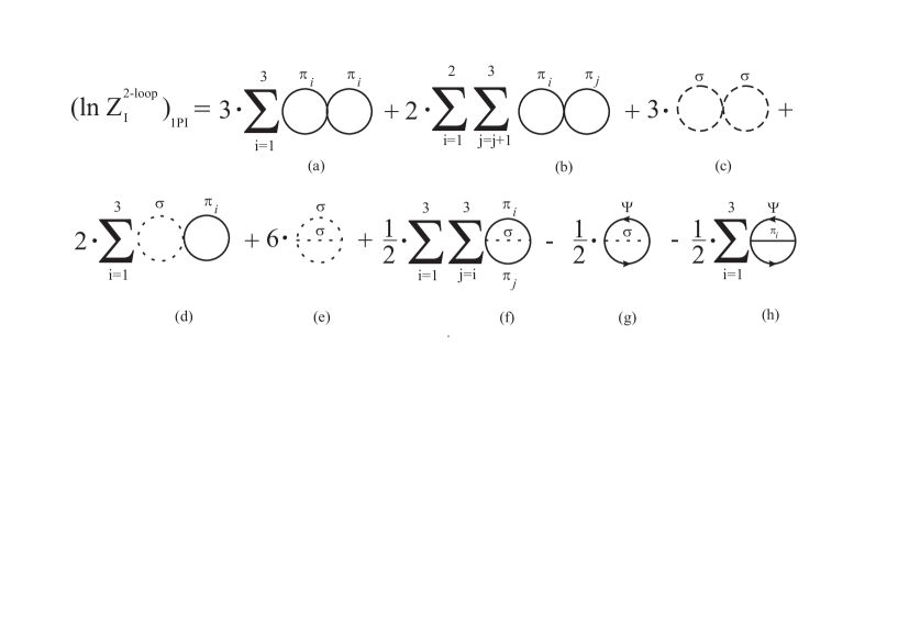
Refer to caption

FIG. 1.: Figure 1: The logarithm of the interaction partition function 1PI. Solid line is the tree-level pion meson propagator, the dashed line is the tree-level sigma meson propagator and the solid line with a arrow is the tree-level fermion propagator.

Refer to caption

FIG. 2.: Figure 2: One-loop self-energy for the pions.

Refer to caption

FIG. 3.: Figure 3: One-loop self-energy for the meson sigma.

Refer to caption

FIG. 4.: Figure 4: One-loop self-energy for the fermions. Note that the lowest corrections for the fermions are of order g2superscript𝑔2g^{2}.

Refer to caption

FIG. 5.: Figure 5: (a) The 1PI one-loop self-energy diagram of the λϕ4𝜆superscriptitalic-ϕ4\lambda\phi^{4} model and (b) a “daisy” type diagram with three attached bubbles which contributes to the self-energy.

Refer to caption


FIG. 6.: Figure 6: Tree-level resumed meson masses.

Refer to caption

FIG. 7.: Figure 7: Tree-level resumed fermion mass.

Refer to caption

FIG. 8.: Figure 8: Condensate ν𝜈\nu as a function of the temperature.

Refer to caption

FIG. 9.: Figure 9: Condensate ν𝜈\nu as a function of the temperature in the chiral limit (Mπ=0subscript𝑀𝜋0M_{\pi}=0).