WHAT WE KNOW ABOUT THE THEORETICAL FOUNDATION OF DUALITY IN ELECTRON SCATTERING

Abstract

We consider some of the things that we understand about the theoretical underpinnings of duality, including items such as why the resonance peak/background ratio is constant in general, why it falls for the $\Delta(1232)$, what we might expect for scaling and duality with longitudinal or spin-dependent structure functions, and what kind of scaling or duality we might expect for semiexclusive processes.

1 Introduction

One has to confess that we don’t understand the theoretical foundation of duality in electron scattering. That should not place a total damper on this discussion. We do understand some things, and we will try to explain what we do understand.

In this talk, after some preliminary remarks defining what we mean by duality in electron (or more generally, lepton) scattering, and some further preliminary remarks about why it could be useful to understand duality well, we will examine a number of more specific topics where we do have some understanding or can make predictions, including

• Why, in general, do the resonance peaks stick up above the smooth “background” curve by the same ratio regardless of the momentum transfer involved?

• Why would a specific resonance like the $\Delta(1232)$ be an exception to the above, or, why does the $\Delta(1232)$ disappear?

• What kind of scaling or duality do we expect for the longitudinal structure function?

• What kind of scaling or duality do we expect for data with polarized initial states?

• What kind of scaling or duality can we look for with semi-exclusive data?

We will continue this introduction with the promised remarks, and then in section 2 answer as well as we can the questions posed.

1.1 Statement of duality

One can separate two aspects of duality. One is “local duality,” and the other the the constancy of the resonance peak to background ratio, which can be viewed as discussing how the local duality is realized. “Duality,” if unqualified is often taken to mean local duality.

Local duality, if there if no evolution of the structure function, is constancy of an average of the structure function over a limited $x$ region. Take the brackets $\langle\ldots\rangle$ to mean an average over a region of $x$ that can include some chosen resonance at low $Q^{2}$. Then duality implies equality between $\langle F_{2}(x,Q^{2})\rangle$ evaluated at a low $Q^{2}$, where $F_{2}$ is in the resonance region, to the same quantity and the same $x$ region but at a high $Q^{2}$ in the scaling region.

If there is evolution, one would think one should compare $\langle F_{2}(x,Q^{2})\rangle$ for real data at low $Q^{2}$, in the resonance region, to the same quantity and the same $x$ region but for the smooth scaling curve evolved to the same $Q^{2}$. There is, however, an interesting and unsettled question that we won’t discuss, and that is whether there is reduced $F_{2}$ evolution in the resonance region [1].

Broadly, the appearance of duality in the data tells us that the single quark reaction rate determines accurately the reaction rate for the entire process, including final state interactions—on the average.

1.2 Possible uses of duality

There are useful experimental studies we could undertake if the role of the final state interactions in forming the resonance becomes moot when averaged over, say, the resonance width. If reliably understood, duality could be useful.

• One could study the structure functions in the $x\rightarrow 1$ region. For a fixed available energy, $x\rightarrow 1$ means getting into the resonance region and if one were sure of the connection of the resonance region average to the scaling curve, one could determine the scaling result for $F_{2}$ significantly closer to the kinematic upper endpoint.

• Similar remarks for apply to the semiexclusive reaction, $\gamma^{*}(q)+p\rightarrow\pi(k)+X$, with the pion emerging with 3-momentum parallel to that of the virtual photon, as proposed by C. Armstrong et al.

We will now proceed to a few more specific points about what is known and what could further be studied in exclusive-inclusive connections in electron scattering. We should remark that there has been a “proof”, or at least a “demystification,” of duality in an interesting paper by DeRújula, Georgi, and Politzer in 1977 [2]. There seems, however, room for more discussion.

2 Discussion

2.1 Why constant signal/background or resonance/continuum (in general)?

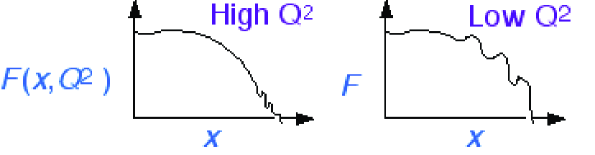
Figure 1: Scaling curves, with locations of resonance bumps at low and high $Q^{2}$.

There always is a resonance region. As $Q^{2}$ increases it slides closer to the kinematic endpoint $x=1$. We may ask, using the language that the “signal” is the resonance peak “continuum” is gotten from the scaling curve, whether or not we expect the signal to continuum ratio to be constant—as it often appears to be in Nature?

Note that this question is logically independent of local duality. One way to realize local duality is allows a constant signal to continuum ratio. But local duality could also be realized by having the resonance disappear into the background beneath it, with the total averaging out in a way that preserves local duality. Conversely, the resonance peak could be very large, with the average unequal to what is obtained from the scaling curve, and yet the signal/continuum ratio be constant.

To return to the question, it does appear we can prove that within perturbative QCD we do expect a constant signal to continuum ration [3]. The proof has one requirement each on the scaling curve and the resonance production form factors, namely

• a $(1-x)^{3}$ behavior for scaling curve as $x\rightarrow 1$ (which can itself be proved in perturbative QCD), and

• pQCD scaling (in $Q^{2}$) of the leading (helicity conserving) resonance form factor

The proof was written out in the live version of these notes, and may be examined in [3]. Basically, it proceeds by writing the cross section for production of a resonance with finite width, switching variables from $Q^{2}$ (for example, in the nucleon to resonance transition form factors) to $x$, and then comparing the result to the deep inelastic cross section to recognize the connection between $F_{2}$ and the form factors. The result works for most known resonances.

2.2 Why the Delta(1232) disappears

The $\Delta(1232)$, unlike resonances in the 1535 or 1688 MeV regions, becomes progressively harder to find as $Q^{2}$ increases. This violates the theorem whose proof was just outlined, and one would like to know why.

First, however, let us point out that local duality is still maintained. Duality means that the average over the resonance region matches the the average using the scaling curve. It does–even for $\Delta(1232)$. What happens is that as the resonance peak falls, the background rises, and average/continuum $\approx$ const. [4]

One concludes that the background knows about the $\Delta$, and co-concludes that one should not use just simple $\pi$-nucleon Born terms to model the background.

Why $\Delta$ disappears is simply because the asymptotic size of the leading helicity form factor is anomalously small. This is not just a result of observation, but also a result of a pQCD calculation, similar to the better known pQCD calculation of the high $Q^{2}$ nucleon elastic dirac form factor $F_{1}$.

Figure 2: Example of lowest order diagram that underlies pQCD form factor calculation.

Hence what we mainly see in $N\rightarrow\Delta$ are asymptotically subleading amplitudes. It is a lousy circumstance for pQCD that the first resonance is an exceptional case, yet it is a circumstance substantiated by calculation.

2.3 The longitudinal structure function

We will just assert that we still expect duality to work. In particular, we expect the signal to continuum ratio is the same at all $Q^{2}$, just as it is for $F_{2}$, which is dominantly the transverse structure function. This assertion follows a prediction of pQCD, this time given [3]

• a $(1-x)^{4}$ behavior for the longitudinal structure function scaling curve as $x\rightarrow 1$ (again itself a result of pQCD), and

• pQCD scaling (in $Q^{2}$) of resonance form factor for longitudinal photons (one quark helicity flip)

But there may be some differences. For example,

• The signal to continuum ratio may be constant even for the $\Delta(1232)$ That the leading helicity amplitude is anomalously small does not mean that the next-to-leading helicity amplitude (which is not currently calculable in pQCD) is also small. If it is normal size, the $\Delta(1232)$ will not be a disappearing resonance in the longitudinal channel.

• Maybe the Roper, the $N(1440)$, will appear. It has not been observed in electroproduction when measuring the transverse channel. There is an interesting possibility that if the Roper is hybrid baryon (meaning its lowest significant Fock component is a qqqg state), its leading electroproduction amplitude is asymptotically $1/Q^{2}$ smaller than qqq, but its longitudinal amplitude has normal falloff [5].

2.4 Expectation with polarized initial states

We expect duality to work for spin dependent structure function, $g_{1}$, also. Time was, and space is, short, and so we shall just refer to reference [6] and the work of X. Ji et al. [7].

2.5 What to look for with semi-exclusive data

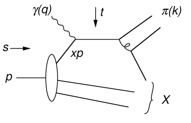
Figure 3: Direct or short distance pion production.

In

$$\gamma(q)+p\rightarrow\pi(k)+X,$$

if the pion is produced in a direct or short range process, illustrated in Fig. 3, then we can show that there will be a function [8], $F(x,s,t,q^{2})$, for which there will be a scaling region where it is dependent mainly on $x$,

$$x\equiv{-t\over s+u-2m_{N}^{2}-q^{2}-m_{\pi}^{2}},$$

where $s$, $t$, and $u$ are Mandelstam variables, and—at least for the direct process—$x$ is the momentum fraction of the struck quark [9, 11], just as in deep inelastic scattering.

For scaling, one needs $s$, $t$, $u$, and $m_{X}$ large. We can get $m_{X}$ into the resonance region with fixed $q^{2}$ and diminishing $t$. Will we see an inclusive-exclusive connection as in the DIS case?

First we have to see scaling, which in addition to requiring large values of the kinematic variables also requires that the competing processes, such as the soft or vector meson dominated (VMD) process and fragmentation (illustrated in Fig. 4), be small.

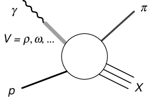
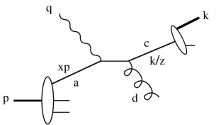
Figure 4: A vector meson dominated and a fragmentation process.

VMD is a serious background for photoproduction with 12 GeV photons. We can decrease the size of VMD process by using spacelike off-shell photons, rather than real photons, since

$${1\over m_{\rho}^{2}}\rightarrow{1\over Q^{2}+m_{\rho}^{2}}$$

We have from earlier work the means to calculate direct process [9] and estimate VMD process [10]. A preliminary result for $\gamma(q)+p\rightarrow\pi^{+}(k)+X$ is shown in Fig. 5 for electroproduction where we have chosen the incoming photons to have and energy of 12 GeV and to be off-shell by 1 GeV² spacelike. The straight lines show several different lab angles for the outgoing pion, and the small triangles are crucial marks. Above and to the right of the triangles, direct or short distance pion production dominates over VDM or fragmentation processes, so that in this region we can connect an experimentally measurable $x$ to the momentum fraction of the struck quark, define a scaling function, and then follow what happens as we enter the resonance region. The solid curved lines, which one can show are ellipses, show the boundaries for $m_{X}$ being $m_{N}$, 2 Gev, and 3 GeV. The region between the outer two curves is the resonance region, and inside the $m_{X}=2$ GeV curve is the scaling region. There is also one curve, a dashed ellipse, showing the path of constant $x=0.5$ in this diagram.

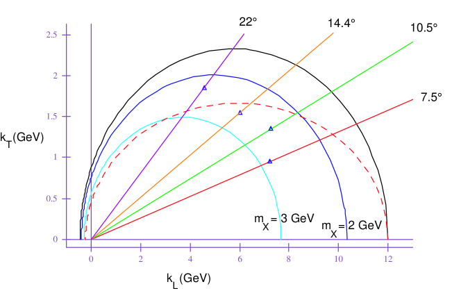
Figure 5: Kinematic regions for $\gamma(q)+p\rightarrow\pi^{+}(k)+X$. Direct or short distance processes dominate above and to the right of the small triangles. The solid ellipses show $m_{X}=m_{N}$, 2 GeV, 3 GeV. The dashed ellipse is for fixed $x=0.5$.

Thus the kinematics exists for allowing a study of some function $F(x,s,t,q^{2})$ which should scale in the region $m_{X}>2$ GeV and high $Q^{2}$, and one can see if it too exhibits the properties of local duality and constant signal to continuum ratio as one enters the resonance region.

References

References

- [1] See e.g., S. J. Brodsky, T. Huang, and G. P. Lepage, Proceedings of the Banff Summer Institute on Particles and Fields, Banff, Canada, Aug. 16-27, 1981, edited by A. Z. Capri and A. N. Kamal (Plenum Press, 1983), pp. 143-199 (see especially pp. 177-178).
- [2] A. DeRújula, H. Georgi, and H. D. Politzer, Ann. Phys. (N. Y.) 103, 315 (1977).
- [3] C. E. Carlson and N. C. Mukhopadhyay, Phys. Rev. D 41, 2343 (1990).
- [4] C.E. Carlson and N.C.Mukhopadhyay, Phys. Rev. D 47 (1993) R1737.
- [5] C.E. Carlson and N.C.Mukhopadhyay, Phys. Rev. Lett. 67, 3745 (1991).
- [6] C.E. Carlson and N.C.Mukhopadhyay, Phys. Rev. D 58, 094029 (1998).
- [7] Xiangdong Ji and Jonathan Osborne, hep-ph/9905410.
- [8] A. Afanasev, C. E. Carlson, and C. Wahlquist, hep-ph/0002271.
- [9] A. Afanasev, C. E. Carlson, and C. Wahlquist, Phys. Lett. B 398, 393 (1997) and Phys. Rev.D 58, 054007 (1998).
- [10] A. Afanasev, C. E. Carlson, and C. Wahlquist, Phys. Rev.D 61, 054007 (2000).
- [11] S. J. Brodsky, M. Diehl, P. Hoyer, S. Peigne, Phys. Lett. B 449, 306 (1999).