Abstract

A coupled channel model is used to study the nature of the scalar mesons produced in the decay $\phi\to\gamma\pi\pi$. The $K\bar{K}$ molecular picture of $f_{0}(980)$ is found to be in a good agreement with the recent experimental data from SND and CMD-2. The structure of the light scalar mesons is elucidated by investigating the $S$-matrix poles and the $q\bar{q}$ spectral density.

1 Introduction

The production of scalar mesons in radiative decays is a valuable source of information on hadron spectroscopy. It was argued [1, 2] that the branching ratio for $\phi\to\gamma f_{0}(980)$ can be used to make a unique choice among different models of $f_{0}(980)$: a conventional quark-antiquark state, an exotic $qq\bar{q}\bar{q}$ state [3], and a $K\bar{K}$ molecule [4]. Such a possibility to resolve the long debated problem of the $f_{0}(980)$ structure using a single partial width looks very attractive. However, it was argued in [5] that the dependence of the theoretical predictions for the $\phi\to\gamma f_{0}(980)$ decay on the $f_{0}(980)$ structure is partly due to differences in modeling. Recent measurements of the radiative decays $\phi\to\gamma\pi^{0}\pi^{0}$ by SND [6] and $\phi\to\gamma\pi^{+}\pi^{-},\gamma\pi^{0}\pi^{0}$ by CMD-2 [7, 8] in Novosibirsk have made it possible to confront alternative models of the light scalar mesons with experimental data.

The goal of this paper is to reanalyze the calculation of the decay width for $\phi\to\gamma f_{0}(980)$ in coupled channel models where the $f_{0}(980)$ state arises as a dynamical state (a $K\bar{K}$ molecule which may also have a substantial admixture of a quark-antiquark component). Since the $\phi$ meson is nearly a pure $s\bar{s}$ state, the decay $\phi\to\gamma\pi\pi$ is an OZI–rule violating process which is expected to proceed via a two–step mechanism with intermediate $K\bar{K}$ states. Therefore this decay is well suited for probing the $K\bar{K}$ content of the scalar mesons. The $K\bar{K}$ molecular state was originally proposed in the potential quark model [4, 9, 10]. A dynamical state close to $K\bar{K}$ threshold is also introduced in the coupled channel models [11, 12, 13, 14] and in the meson exchange interaction models [15, 16]. A state strongly coupled to the $s\bar{s}$ and $K\bar{K}$ channels near the $K\bar{K}$ threshold was as well found in the unitarized quark model [17, 18]. The coupled-channel model derived from the lowest order chiral Lagrangian [19, 20] produces a scalar state dominated by the $K\bar{K}$ channel. General discussions of the nature of the $f_{0}(980)$ can be found in [10, 13, 17, 21, 22, 23] and references therein.

Our approach is based on a coupled channel model (CCM) for the $\pi\pi$ and $K\bar{K}$ systems which is similar to the one studied in [13]. The calculation of the decay $\phi\to\gamma f_{0}(980)$ for point-like particles is summarized in Sec. 2. The details of the coupled channel model are given in Sec. 3, and the model parameters are determined from a fit to the $\pi\pi$ scattering data. The reaction $\phi\to\gamma\pi\pi$ in a CCM framework is studied in Sec. 4. The analytic structure of the $\pi\pi$ and $K\bar{K}$ scattering amplitudes is investigated in Sec. 5. The mixing between the two–meson and $q\bar{q}$ channels is discussed in Sec. 6. In Sec. 7 the physical properties of the scalar mesons in the model proposed are discussed and compared to other approaches in the literature. The details of the formalism are collected in the Appendices.

2 The Decay $\phi\to\gamma f_{0}$

For the benefit of the reader, we begin with a brief summary of the formulas describing radiative transitions between vector and scalar states. The amplitude of the radiative $\phi$ decay into the scalar meson $f_{0}$ has the following structure which is imposed by gauge invariance:

$$M(\phi\to\gamma f_{0}) = \epsilon_{\phi}^{\mu}\epsilon_{\gamma}^{\nu}(p_{\nu}q_{\mu}-g_{\nu\mu}(p\cdot q))H(p^{2},(p-q)^{2})$$ (1)

where ($\epsilon_{\phi}$, $p$) and ($\epsilon_{\gamma}$, $q$) are the polarizations and four-momenta of the $\phi$ and $\gamma$, correspondingly, and $H(p^{2},(p-q)^{2})$ is the scalar invariant amplitude which depends on the invariant masses of the initial and final mesons. The polarization vectors satisfy the constraints $\epsilon_{\phi}\cdot p=0$ and $\epsilon_{\gamma}\cdot q=0$. Using the three-dimensional gauge $\epsilon_{\gamma}=(0,\mbox{\boldmath$\varepsilon$}_{\gamma})$ in the center-of-mass system (CMS) one gets the amplitude

$$M(\phi\to\gamma f_{0}) = (\mbox{\boldmath$\varepsilon$}_{\phi}\mbox{\boldmath$\varepsilon$}_{\gamma})m_{\phi}\omega H(p^{2},(p-q)^{2})$$ (2)

where $m_{\phi}$ is the $\phi$ mass, $\omega$ is the photon energy in the CMS, and $\mbox{\boldmath$\varepsilon$}_{\phi}$ and $\mbox{\boldmath$\varepsilon$}_{\gamma}$ are the $\phi$ and $\gamma$ three–dimensional polarization vectors in the CMS, respectively.

(a)                                                                       (b)

     

Figure 1: The minimal gauge-invariant set of diagrams for the decay $M(\phi\to\gamma f_{0})$ in the case of point-like particles: (a) the loop radiation; (b) the contact term.

For point-like particles, the amplitude $M(\phi\to\gamma f_{0})$ is given by the diagrams in Fig.1 (see [5] and references therein). While the diagram Fig.1(a) corresponding to loop radiation is overall logarithmically divergent, its contribution to the $p_{\nu}q_{\mu}$ term in Eq.(1) is finite. Gauge invariance enforces the appearance of the seagull diagram Fig.1(b) which contributes only to the $g_{\nu\mu}(p\cdot q)$ term in Eq.(1). Since the sum of the loop–radiation and seagull terms is gauge invariant, one obtains the total amplitude $M(\phi\to\gamma S)$ by calculating only the $p_{\nu}q_{\mu}$ term of the loop radiation. The result for the scalar invariant amplitude is [24]

$$H(p^{2},(p-q)^{2}) = \frac{eg_{\phi}g_{f_{0}KK}}{2\pi^{2}m_{K}^{2}}I(a,b)$$ (3)

$$a=\frac{m_{\phi}^{2}}{m_{K}^{2}} b=\frac{m_{f_{0}}^{2}}{m_{K}^{2}}$$ , (4)

where $g_{\phi}$ and $g_{f_{0}KK}$ are the $\phi K^{+}K^{-}$ and $f_{0}K^{+}K^{-}$ coupling constants and the function $I(a,b)$ is defined in Appendix A. The radiative decay width is

$$\Gamma(\phi\to\gamma f_{0}) = \frac{\omega^{3}|H(p^{2},(p-q)^{2})|}{12\pi}=$$ (5)

$$= \frac{\alpha g_{\phi}^{2}g_{f_{0}KK}^{2}}{3(2\pi)^{4}}\frac{\omega}{m_{\phi}^{2}}|(a-b)I(a,b)|^{2}\quad.$$ (6)

The generalization of Eqs. (1,3,6) to the case $\phi\to\gamma\pi\pi$ where the $\pi\pi$ system has total angular momentum $J=0$ and isospin $I=0$ is straightforward [25]:

$$M(\phi\to\gamma\pi\pi) = \epsilon_{\phi}^{\mu}\epsilon_{\gamma}^{\nu}(p_{\nu}q_{\mu}-g_{\nu\mu}(p\cdot q))H_{\pi\pi}(p^{2},(p-q)^{2})\quad.$$ (7)

Here the scalar invariant amplitude $H_{\pi\pi}(p^{2},(p-q)^{2})$ is given by (compare with Eq.(3))

$$H_{\pi\pi}(p^{2},(p-q)^{2}) = \frac{eg_{\phi}}{2\pi^{2}m_{K}^{2}}I(a,b)\;t_{K^{+}K^{-}-\pi\pi}$$ (8)

and $t_{K^{+}K^{-}-\pi\pi}$ is the $J=0$ part of the $T$-matrix for the $K^{+}K^{-}\to\pi\pi$ scattering. The $\pi\pi$ invariant mass distribution has the form

$$\frac{d\Gamma}{dM_{\pi^{+}\pi^{-}}}=2\frac{d\Gamma}{dM_{\pi^{0}\pi^{0}}} = \frac{\alpha g_{\phi}^{2}\;\omega}{18(2\pi)^{6}m_{\phi}^{2}}|(a-b)I(a,b)|^{2}|t^{0}_{K\bar{K}-\pi\pi}|^{2}k_{\pi\pi}$$ (9)

where $t^{0}_{K\bar{K}-\pi\pi}=\sqrt{6}\;t_{K^{+}K^{-}-\pi^{+}\pi^{-}}$ is the isoscalar $K\bar{K}\to\pi\pi$ amplitude and $k_{\pi\pi}$ is the relative momentum of the pions in the final state:

$$k_{\pi\pi} = \sqrt{M_{\pi\pi}^{2}/4-m_{\pi}^{2}}\quad,\quad M_{\pi\pi}^{2}=(p-q)^{2}\quad.$$ (10)

Equation (9) leads to Eq.(6) in the Breit–Wigner (BW) approximation for the $K^{+}K^{-}\to\pi\pi$ scattering amplitude

$$t_{K^{+}K^{-}-\pi\pi} = \frac{g_{f_{0}KK}g_{f_{0}\pi\pi}}{M_{\pi\pi}^{2}-(M_{f_{0}}-i\Gamma_{f_{0}}/2)^{2}}$$ (11)

under the assumption that the integral over the $\pi\pi$ mass spectrum is saturated by the narrow resonance with mass $M_{f_{0}}$ and width $\Gamma_{f_{0}}$ (see Appendix A).

According to Eq.(8), the hadronic part of the amplitude, which contains the information about the scalar mesons, is factored out in the form of the $T$-matrix for the $K^{+}K^{-}\to\pi\pi$ scattering, with both the physical region ($M_{\pi\pi}\geq 2m_{K}$) and the unphysical region ($M_{\pi\pi}<2m_{K}$) being relevant to the $\phi\to\gamma\pi\pi$ decay. It is known from the studies of scalar mesons, see [13, 22, 23, 26] and references therein, that the analytical structure of the scalar–isoscalar amplitudes near the $K\bar{K}$ threshold is far from being a trivial BW resonance. Therefore a coupled channel model of the $K^{+}K^{-}\to\pi\pi$ scattering is required to describe the decay $\phi\to\gamma\pi\pi$ beyond the BW approximation.

3 The $\pi\pi-K\bar{K}$ Coupled Channel Model

To describe the interaction in the $\pi\pi-K\bar{K}$ system with total angular momentum $J=0^{++}$ and isospin $I^{G}=0^{+}$ we exploit a coupled channel model similar to that of [13]. The two scattering channels, 1 and 2, correspond to the $\pi\pi$ and $K\bar{K}$ systems and channel 3 contains a single $q\bar{q}$ bound state. The $T$-matrix, as a function of the invariant mass squared $s$, is defined by the Lippmann-Schwinger equation

$$\mbox{\boldmath$T$}(s) = \mbox{\boldmath$V$}+\mbox{\boldmath$V$}\mbox{\boldmath$G$}^{0}(s)\mbox{\boldmath$T$}$$ (12)

where $\mbox{\boldmath$G$}^{0}(s)$ is the free Green function.

The interaction potentials are taken in separable form:

$$V = \left(\matrix{v_{11}(s)|1\rangle\langle 1|&v_{12}(s)|1\rangle\langle 2|&g_{13}|1\rangle\langle q\bar{q}|\cr v_{12}(s)|2\rangle\langle 1|&v_{22}(s)|2\rangle\langle 2|&g_{23}|2\rangle\langle q\bar{q}|\cr g_{13}|q\bar{q}\rangle\langle 1|&g_{23}|q\bar{q}\rangle\langle 2|&0\cr}\right)$$ (13)

where the form factors in channel 1 and 2 depend on the corresponding relative three–momentum $k$:

$$\langle k|1\rangle = \xi_{1}(k)=\frac{\lambda_{1}^{2}}{k^{2}+\lambda_{1}^{2}}$$ (14)

$$\langle k|2\rangle = \xi_{2}(k)=\frac{\lambda_{2}^{2}}{k^{2}+\lambda_{2}^{2}}$$ (15)

In [13], the potentials $v_{ij}(s)$ were assumed to be energy independent, and the chiral symmetry constraints on the scattering amplitude were strictly imposed only in the $\pi\pi$ channel by adjusting the strength of $v_{11}$ so that the Adler zero is at the correct position. In the present case, it is essential to ensure a correct behaviour of the $K\bar{K}-\pi\pi$ scattering amplitude not only in the physical scattering region but also down to the $\pi\pi$ threshold. We found it easier to impose the chiral symmetry constraints by using energy dependent potentials. The energy dependence is taken in the form

$$v_{11}(s) = b-g_{11}s$$ (16)

$$v_{12}(s) = -g_{12}s$$ (17)

$$v_{22}(s) = -g_{22}s\quad.$$ (18)

With our choice of interaction (13-18) the analytical solution for the $T$-matrix can be easily obtained. Further details of the model are given in Appendix B. As in [13] we assume that the diagonal interaction in the $K\bar{K}$ channel produces a weakly bound state in the absence of coupling to the other channels, thus simulating a “molecular” origin of the $f_{0}(980)$ resonance. The state $|q\bar{q}\rangle$ in channel 3 has a bare mass $M_{r}>2m_{K}$.

(a)                                                              (b)

     

Figure 2: The scattering phase $\delta_{0}^{0}$ and the inelasticity parameter $\eta_{0}^{0}$ for the $S$-wave $\pi\pi$ scattering vs. the $\pi\pi$ invariant mass. The experimental points are from [27, 28, 29]. The curves show the fits in our model: fit 1 (the dashed lines) involves only the $\pi\pi$ scattering data, fit 4 (the solid lines) includes in addition the data for $\phi\to\gamma\pi^{0}\pi^{0}$ [6, 8].

Table 1: The model parameters obtained from the data fits. The fit 1 is based on using only the $\pi\pi$ scattering data (the phase $\delta_{0}^{0}$ and the inelasticity $\eta_{0}^{0}$). The fits 2–4 include in addition the mass distribution $d\Gamma/dM_{\pi\pi}$ in the decay $\phi\to\gamma\pi^{0}\pi^{0}$: data from SND [6] in fit 2, from CMD-2 [8] in fit 3, and the combined data [6, 8] in fit 4. The value of $\lambda_{2}$ was fixed in all fits.

fit	$b$	$g_{11}$	$g_{22}$	$g_{12}$	$\lambda_{1}$	$\lambda_{2}$	$g_{13}$	$g_{23}$	$M_{r}$
	GeV-1	GeV-3	GeV-3	GeV-3	GeV	GeV	GeV1/2	GeV1/2	GeV
(1)	5.251	3.564	5.326	3.741	0.477	0.7	2.670	0.464	1.136
(2)	6.075	2.953	3.945	-0.121	0.499	0.7	2.708	0.716	1.094
(3)	5.188	2.944	3.683	-0.270	0.538	0.7	2.576	0.690	1.111
(4)	5.299	2.954	3.725	-0.341	0.529	0.7	2.588	0.702	1.105

Figure 3: The $\pi\pi$ invariant mass distribution in the decay $\phi\to\gamma\pi^{0}\pi^{0}$. The curves are the results from our model: the dashed line corresponds to fit 1, the solid line to fit 4. The experimental points are from [6] and [8].

Figure 4: The $T$–matrix for the $K\bar{K}-\pi\pi$ scattering ($J=I=0$) vs. the invariant mass of the $\pi\pi$ system $M_{\pi\pi}$. The model parameters correspond to the fit 4 in Table 1.

The model parameters have been determined from the fit of the $\pi\pi$ scattering phase $\delta_{0}^{0}$ and the inelasticity parameter $\eta_{0}^{0}$ in the mass range $M_{\pi\pi}\leq 1.5\;$GeV, see Table 1 and Figs.2(a,b). Since the fit was found to be only weakly sensitive to the form–factor parameter $\lambda_{2}$, its value was fixed, and only the coupling constants $g_{ij}$, the bare mass of $q\bar{q}$, and $\lambda_{1}$ were treated as free parameters. The parameter $b$ in the diagonal $\pi\pi$ potential Eq.(16) was used for fine tuning of the $\pi\pi$ scattering length which was fixed at $a_{0}^{0}=0.22m_{\pi}^{-1}$. The best fit of only the $\pi\pi$ scattering data (fit 1) does not lead automatically to a very good description of the $\pi\pi$ invariant mass distribution in the decay $\phi\to\gamma\pi\pi$. However, the shape of the $\phi\to\gamma\pi\pi$ improves if the $d\Gamma/dM_{\pi\pi}$ data are added to the fit as shown in Fig.3 (the details are discussed in Sec.4). As a result, our model provides a good description of the whole data set.

The energy dependence of the $T$-matrix element $t_{K^{+}K^{\to}\pi\pi}$ calculated in our coupled channel model is shown in Fig.4. In addition to a narrow peak due to the $f_{0}(980)$ state, this matrix element has a significant contribution from the lower mass region corresponding to the $\sigma$ meson.

4 The Decay $\phi\to\gamma\pi\pi$ in the Coupled Channel Model

(a)                                         (b)                                         (c)

           

Figure 5: The minimal set of diagrams giving a gauge-invariant amplitude $M(\phi\to\gamma\pi\pi)$ in the coupled channel model: (a) the loop radiation; (b) the contact (seagull) term, (c) the form factor term. In the nonrelativistic approximation, the particles marked with $\times$ are on mass shell.

(a)                                                                       (b)

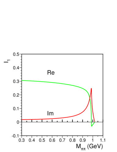
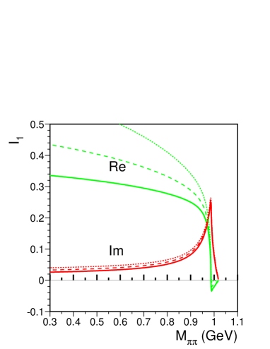
Figure 6: (a) The function $I_{1}=(a-b)I(a,b)$, $a=m_{\phi}^{2}/m_{K}^{2}$, $b=M_{\pi\pi}^{2}/m_{K}^{2}$ vs. the invariant mass of the $\pi\pi$ system $M_{\pi\pi}$.  (b) Its nonrelativistic analog $J_{\lambda}(M_{\pi\pi})\cdot(m_{\phi}^{2}-M_{\pi\pi}^{2})/m_{K}^{2}$ for $\lambda=0.5\;$GeV (solid lines), $\lambda=0.6\;$GeV (dashed lines), and $\lambda=0.8\;$GeV (dotted lines).

The formulas given in Sec. 2 are valid for point-like particles. When a form factor in the $K\bar{K}-\pi\pi$ vertex is included, the $\phi\to\gamma\pi\pi$ amplitude contains an additional term arising from the minimal substitution $k_{\mu}\to(k_{\mu}-eA_{\mu})$ in the momentum dependence of the form factors (see [5] for details). With an appropriate choice of the form factors, the sum of three diagrams shown in Fig. 5 becomes explicitly finite. In order to study the influence of the form factors on the results for the $\phi\to\gamma\pi\pi$ we use a nonrelativistic approximation for the $K^{+}$ and $K^{-}$, which is justified by the fact that the most interesting region corresponding to the $f_{0}(980)$ resonance is very close to the $K\bar{K}$ threshold. The electric dipole matrix element is factorized into two parts describing the $K^{+}K^{-}$ loop radiation with gauge invariant complement and the final state rescattering $K^{+}K^{-}\to\pi\pi$, correspondingly. The total scalar invariant amplitude has the form

$$H_{\pi\pi}^{(\lambda)}(p^{2},q^{2}) = \frac{eg_{\phi}}{2\pi^{2}m_{K}^{2}}J_{\lambda}(M_{\pi\pi})t_{K^{+}K^{\to}\pi\pi}(M_{\pi\pi})$$ (19)

which is similar to the relativistic point-like case defined by Eq.(8) where the function $I(a,b)$ is replaced by $J_{\lambda}(M_{\pi\pi})$. For the definition of $J_{\lambda}(M_{\pi\pi})$ and further technical details we refer to Appendix C. The parameter $\lambda$ refers to the form–factor dependence on the relative $K^{+}K^{-}$ momentum in the $K^{+}K^{-}\to\pi\pi$ vertex given by Eq.(15). Figure 6 shows the dependence of the electric dipole matrix element on the $\pi\pi$ invariant mass for different values of the form–factor parameter $\lambda$ in comparison with the relativistic point-like case.

With our choice of the form factor (15) there is no substantial suppression of the nonrelativistic result in comparison to the point-like case for the relevant range of $\lambda=0.6-0.8\;$GeV (which corresponds to the data fit in our coupled channel model). For larger values of $\lambda$, the full relativistic treatment is needed as the real part of the nonrelativistic result becomes sensitive to the short distance contribution (see the discussion in [5]). The dependence of the imaginary part of $M(\phi\to\gamma\pi\pi)$ on the form factor in the mass region close to the $K\bar{K}$ threshold is rather weak. As a result, we can neglect the form–factor dependence in the loop calculations and just use the relativistic point–like result given by Eq.(8). It is interesting to note that the imaginary part can be obtained from the divergent triangle diagram Fig.5(a) alone by using the Siegert theorem which ensures a correct behaviour of the electric dipole matrix element.

5 The Poles of the $S$-Matrix

The poles of the $S$-matrix in the complex $s$-plane corresponding to the fits in Sect.3 are shown in Table 2 and Fig.7. There are five poles related to the resonances in our model. The pole $M_{A}$ located on the sheet II (${\mathrm{I}m}\;k_{1}<0$, ${\mathrm{I}m}\;k_{2}>0$) is very close to the $K\bar{K}$ threshold. The pair of poles, $M_{B}$ on sheet II and $M_{D}$ on the sheet III (${\mathrm{I}m}\;k_{1}<0$, ${\mathrm{I}m}\;k_{2}<0$), corresponds to a broad structure associated with the $\sigma$ meson. The other pair of poles, $M_{C}$ on sheet II and $M_{E}$ on sheet III, corresponds to a broad resonance above the $K\bar{K}$ threshold, which can be associated with the $f_{0}(1370)$ state (for a more realistic description of the $S$-matrix above 1.3 GeV additional poles are needed which are not included in the present model). The position of the resonance poles depends on the coupling constants, and this distinguishes them from the fixed poles originating from the singularities of the form factors (15). The latter are located at $k_{1}=\pm i\lambda_{1}$ and $k_{2}=\pm i\lambda_{2}$, their distance to the physical region being determined by the range of the interaction. In our model these fixed poles approximate the potential singularities which correspond to the left hand cut in a more general case.

Table 2: The resonance poles of the $S$-matrix in the complex mass plane $M=\sqrt{s}$ (GeV). The definition of the fits is given in Table 1.

Pole	Sheet	fit 1	fit 2	fit 3	fit 4
$M_{A}$	II	$0.991-i0.024$	$0.974-i0.020$	$0.978-i0.015$	$0.975-i0.017$
$M_{B}$	II	$0.455-i0.237$	$0.456-i0.232$	$0.469-i0.234$	$0.465-i0.236$
$M_{C}$	II	$1.214-i0.262$	$1.401-i0.266$	$1.424-i0.261$	$1.417-i0.263$
$M_{D}$	III	$0.789-i0.487$	$0.677-i0.234$	$0.670-i0.266$	$0.666-i0.227$
$M_{E}$	III	$1.403-i0.320$	$1.384-i0.261$	$1.408-i0.250$	$1.400-i0.249$

(a)

(b)                                                              (c)

Figure 7: (a) The trajectories of the $S$-matrix poles (fit 4) in the complex mass plane (GeV) on the sheets II and III for the $K\bar{K}-\pi\pi$ and $q\bar{q}-\pi\pi$ couplings increasing from $x=0$ to the physical values $x=1$. (b) The magnified region of the $f_{0}(890)$ resonance. (c) The $\sigma$ meson trajectory in the complex plane of the $\pi\pi$ relative momentum $k_{1}$ (GeV) with (solid line) and without (dashed line) coupling to the $q\bar{q}$ state.

The origin and the nature of the resonance poles found in our model can be elucidated by studying how these poles move in the complex $s$-plane when the model parameters are varied between the physical case determined by the fit and the limit of vanishing couplings in the $\pi\pi$ channel and between the $\pi\pi$ and the other channels ($K\bar{K}$ and $q\bar{q}$):

$$v_{11}(s) \to x\cdot v_{11}(s)\quad,\quad 0\leq x\leq 1$$ (20)

$$v_{12}(s) \to x\cdot v_{12}(s)$$ (21)

$$g_{13} \to x^{1/2}\cdot g_{13}$$ (22)

$$g_{23} \to x^{1/2}\cdot g_{13}$$ (23)

The diagonal interaction in the $K\bar{K}$ channel with the physical strength of the coupling $g_{22}$ produces a bound state close to the $K\bar{K}$ threshold with mass $m_{K\bar{K}}=0.97\;$GeV.

(a)                                                                       (b)

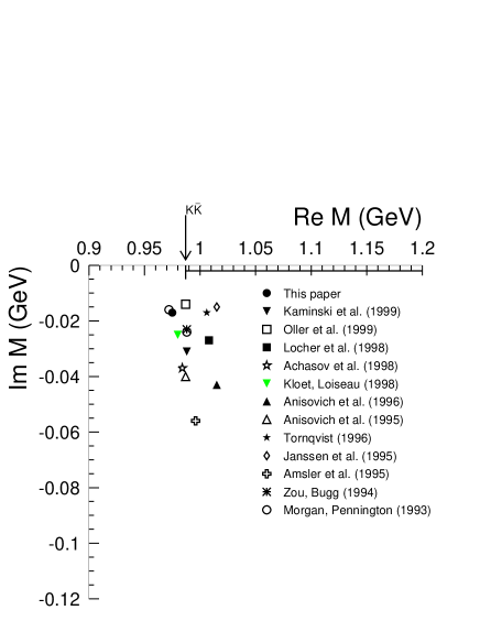
Figure 8: The poles of the $S$-matrix corresponding to the $f_{0}(980)$ in different models [6, 14, 13, 16, 18, 20, 22, 31, 33, 35, 36, 37]: (a) sheet II pole ($\mbox{Im}\;k_{1}>0$, $\mbox{Im}\;k_{2}<0$) and (b) sheet III pole ($\mbox{Im}\;k_{1}<0$, $\mbox{Im}\;k_{2}<0$).

Our coupled channel model has only one pole $M_{A}=0.975-i0.017\;$GeV near the $K\bar{K}$ threshold, which is sufficient for a good description of the $\pi\pi$ scattering data. This pole is directly related to a molecular $K\bar{K}$ state in the absence of coupling to the $\pi\pi$ channel. The number of the $S$-matrix poles near the $K\bar{K}$ threshold has been discussed in the literature (see [13, 22, 26] and references therein) for a long time. While the relation of the $f_{0}(980)$ meson to at least one $S$-matrix pole close to $K\bar{K}$ threshold is well established, the exact location and even the number of the relevant $S$-matrix poles is model dependent as demonstrated in Fig.8. The models based on dynamical input (coupled channel, potential, unitarized chiral perturbation theory) [11, 12, 14, 16, 17, 19, 30] usually produce only one pole which can be traced to a weakly bound $K\bar{K}$ state in an appropriate limit of the channels coupling. One exception to this observation is a coupled channel model [13] where the second pole near the $K\bar{K}$ threshold results from the interplay of a nearby $q\bar{q}$ pole with dynamical singularities. We were not able to find a good fit with the same feature in our model; the main reason appears to be due to the using of the energy dependent potentials in Eq.(13) contrary to the case in [13]. However, it is not excluded that two–pole solutions can be found with some other parametrization of interactions in CCM. It remains to be investigated whether two–pole solutions are compatible with the data on the $\phi\to\gamma\pi\pi$ decay.

The $K$-matrix parameterizations [22, 26, 31, 32, 33, 34, 35, 36] routinely produce the second pole on sheet III. There is, however, a much larger spread in this pole location than on sheet II. As shown above, the reaction $\phi\to\gamma\pi\pi$ allows one to probe the scattering $K\bar{K}\to\pi\pi$ both above and below the $K\bar{K}$ threshold, and the $\pi\pi$ mass distribution in $\phi\to\gamma\pi\pi$ is very sensitive to the $S$-matrix poles related to the $f_{0}(980)$. Therefore more detailed experimental data on $\phi\to\gamma\pi\pi$ would be very useful for reducing the present uncertainty about the analytical structure of the $S$-matrix in the $f_{0}(980)$ region.

6 The Mixing between the $q\bar{q}$ and Mesonic Channels

(a)                                                              (b)

Figure 9: (a) The spectral density of the $q\bar{q}$ state and (b) the corresponding Laplace transforms.

The mixing of the quark-antiquark states with the open meson channels can be studied in the CCM by using the probability sum rule for a resonance embedded into a continuum [38] which is described in Appendix B. The spectral function $\rho(s)$ which determines the probability density for the $q\bar{q}$ component in the scattering states, as defined by Eq.(56), is shown in Fig.9(a). In the case of weak coupling, the probability density would be well localized near the position of the bare $q\bar{q}$ state at $M_{r}=1.1\;$GeV. For the physical case, we find a broad peak centered above the $K\bar{K}$ threshold in the region corresponding to the $f_{0}(1370)$ resonance (the poles $M_{E}$ and $M_{C}$). There is also a sizable contribution to the $q\bar{q}$ spectral density from the low–mass region of the $\sigma$ meson. The $\rho(s)$ distribution in the $f_{0}(980)$ resonance has a characteristic dip-bump structure resulting from an interplay of the resonance pole $M_{A}$ with a nearby zero of the mass operator $\Pi(s)$. The position and the width of the $\rho(s)$ distribution indicates that an essential contribution to the saturation of the sum rule (56) comes from the pole $M_{B}$ related to the $\sigma$ meson, while the narrow structure associated with the pole $M_{A}$ alone plays a minor role. The fact that $q\bar{q}$ coupling with the $\pi\pi$ channel significantly enhances the spectral density $\rho(s)$ in the region of the $\sigma$ meson is related to the interplay of the $S$-matrix poles demonstrated in Fig.7c: the pole $M_{B}$ corresponding to the $\sigma$ meson is pushed towards the $\pi\pi$ threshold by the pole $M_{C}$ originating from the $q\bar{q}$ state.

Using the spectral density $\rho(s)$ we can calculate the contribution of the $q\bar{q}$ scalar mesons to the QCD sum rule related to the scalar quark condensate [39]. Figure 9b shows the Laplace transform of the spectral density which is used in the sum rule analysis:

$$I_{n}(M^{2}) = \int_{0}^{\infty}s^{n}e^{-s/M^{2}}\rho(s)ds$$ (24)

The advantage of CCM with respect to the previous studies (see [40] and references therein) where the contribution of the $q\bar{q}$ mesons was usually approximated by one narrow resonance is a more realistic shape of the $q\bar{q}$ spectral density in the low-mass region which is important in the Laplace sum rules. As a result, the momenta $I_{0}(M^{2})$ and $I_{1}(M^{2})$ have quite different slopes in their $M^{2}$–dependence as shown in Fig.9(b).

7 Discussion

The theoretical calculations of the decays $\phi\to\gamma\pi\pi$ and $\phi\to\gamma f_{0}(980)$ and the corresponding experimental data are summarized in Table 3. The predicted branching ratios for the $\gamma\pi^{0}\pi^{0}$ and $\gamma\pi^{+}\pi^{+}$ channels should be compared with the experimental data with some caution. While these branching ratios can be easily defined theoretically ($\Gamma_{\phi\to\gamma\pi^{+}\pi^{-}}/\Gamma_{\phi\to\gamma\pi^{0}\pi^{0}}=2$ for the isoscalar $\pi\pi$ states, e.g.), the data analysis relies on the modeling of competing reaction mechanisms. In particular, the interpretation of the experimental results for the $\gamma\pi^{+}\pi^{+}$ channel involves the consideration of the interference between the $e^{+}e^{-}\to\phi\to\gamma\pi\pi$ and $e^{+}e^{-}\to\gamma\rho\to\gamma\pi\pi$ mechanisms. In this respect, we wish to emphasize again the importance of using a realistic $K^{+}K^{-}\to\pi\pi$ amplitude instead of a simple superposition of BW resonances. The channel $\gamma\pi^{0}\pi^{0}$ which is free from the $\rho$ meson contribution in the $\pi\pi$ channel appears to be better suited for the study of the $\pi\pi$ invariant mass distribution, although this case has some background due to the mechanism $\phi\to\pi^{0}\rho^{0}\to\pi^{0}\pi^{0}\gamma$.

Our results are in good agreement with recent calculations within the chiral unitary approach [25] both for the total width and for the $\pi\pi$ mass distribution. This is not surprising because in both cases the $f_{0}(980)$ resonance is produced mainly by the attractive interaction in the $K\bar{K}$ channel. Our result for the total width $\Gamma_{\phi\to\gamma\pi\pi}$ is close to the earlier calculations of the two–step mechanism with the intermediate $K^{+}K^{-}$ state [5, 24] which used the BW approximation (6) with the coupling constant $g_{f_{0}K\bar{K}}^{2}/4\pi=0.6\;\mbox{\rm GeV}^{2}$. In our model we can define an effective coupling constant $g_{f_{0}K\bar{K}}$ by approximating the $K\bar{K}\to\pi\pi$ amplitude (52) by a BW resonance which leads to slightly higher value of $g_{f_{0}K\bar{K}}^{2}/4\pi=1.1\;\mbox{\rm GeV}^{2}$.

The effect of the form factor in the $K\bar{K}\pi\pi$ vertex was studied earlier in [5] where a suppression by a factor of about 5 was given as an estimate. This significant suppression resulted from the use of a very soft dipole form factor with the characteristic parameter $\mu=0.14\;$GeV (Eq.(4.14) in [5]) which was suggested by the study of the $\phi\to\gamma\gamma$ decay [41]. However, the $2\gamma$ decay is related to the short distance behavior of the $K\bar{K}$ wave function, while we are interested in the $\phi K\bar{K}$ vertex at moderate relative momenta (in general, there is no unique relation between these two properties, see the discussion in [41]). It is difficult to justify such a low value of the form–factor parameter in the CCM: a good fit of the scattering data requires much harder form factors as discussed in Sec. 3. A weak effect of the form factor found in our case is consistent with the results in [5] if the form–factor parameter $\mu\geq 0.5\;$GeV is used there.

Reaction	Branching ratio	Ref.
Theory
$\phi\to\gamma f_{0}(980)\to\gamma\pi\pi$	$2.6\cdot 10^{-4}$	[2]
$\phi\to\gamma f_{0}(980)$	$1.9\cdot 10^{-4}$	[24]
$\phi\to\gamma f_{0}(980)$ (point–like)	$1.4\cdot 10^{-4}$	[5]
$\phi\to\gamma f_{0}(980)$ (with form factor)	$0.3\cdot 10^{-4}$	[5]
$\phi\to\gamma(f_{0}+\sigma)\to\gamma\pi\pi$ ($q^{2}\bar{q}^{2}$ model)	$\sim 10^{-4}$	[42]
$\phi\to\gamma(f_{0}+\sigma)\to\gamma\pi\pi$ ($K\bar{K}$ model)	$\sim 10^{-5}$	[42]
$\phi\to\gamma(f_{0}+\sigma)\to\gamma\pi\pi$ ($s\bar{s}$ model)	$\sim 5\cdot 10^{-5}$	[42]
$\phi\to\gamma(\pi^{0}\pi^{0})_{J=0}$	$0.8\cdot 10^{-4}$	[25]
$\phi\to\gamma(\pi^{+}\pi^{-})_{J=0}$	$1.6\cdot 10^{-4}$	[25]
$\phi\to\gamma(\pi^{0}\pi^{0})_{J=0}$	$1.2\cdot 10^{-4}$	this paper
$\phi\to\gamma(\pi^{0}\pi^{0})_{J=0}$, ($M_{\pi^{0}\pi^{0}}>0.9\;$GeV)	$0.34\cdot 10^{-4}$	this paper
$\phi\to\gamma(\pi^{+}\pi^{-})_{J=0}$	$2.3\cdot 10^{-4}$	this paper
Experiment
$\phi\to\gamma(\pi^{0}\pi^{0})_{J=0}$	$(1.14\pm 0.10\pm 0.12)\cdot 10^{-4}$	[6]
$\phi\to\gamma(\pi^{0}\pi^{0})_{J=0}$, ($M_{\pi^{0}\pi^{0}}>0.9\;$GeV)	$(0.5\pm 0.06\pm 0.06)\cdot 10^{-4}$	[6]
$\phi\to\gamma f_{0}(980)$	$(3.42\pm 0.30\pm 0.36)\cdot 10^{-4}$	[6]
$\phi\to\gamma f_{0}(980)$	$(1.96\pm 0.46\pm 0.50)\cdot 10^{-4}$	[7]
$\phi\to\gamma\pi^{0}\pi^{0}$	$(1.08\pm 0.17\pm 0.09)\cdot 10^{-4}$	[8]
$\phi\to\gamma\pi^{0}\pi^{0}$, ($M_{\pi^{0}\pi^{0}}>0.9\;$GeV)	$(0.57\pm 0.06\pm 0.04)\cdot 10^{-4}$	[8]

Table 3: The calculated branching ratios for $\phi\to\gamma(\pi\pi)_{J=0}$ and $\phi\to\gamma f_{0}(980)$ in comparison with the experimental data.

In view of this overall agreement between different calculations of the two–step mechanisms with the $K^{+}K^{-}$ intermediate state we find it difficult to agree with the statements [2, 42] that the $K\bar{K}$ model of $f_{0}(980)$ can be excluded on the ground of its alleged conflict with the $\phi\to\gamma f_{0}(980)$ data. Since the hadronic part of the amplitude $\phi\to\gamma\pi\pi$ is factored out as the matrix element $t_{K\bar{K}-\pi\pi}$ or, in the simplified case, as the coupling constant $g_{f_{0}K\bar{K}}$, the self-consistency of the $K\bar{K}$ model of $f_{0}(980)$ can be examined by analyzing the value of $g_{f_{0}K\bar{K}}$. For this purpose we use a well known result from nonrelativistic scattering theory: the residue of the scattering matrix at a pole corresponding to a bound state is uniquely related to the asymptotic normalization constant of the bound state wave function which for a weakly bound state depends, in leading order, only on the binding energy. For a weakly bound $K\bar{K}$ state, the relation between the $g_{f_{0}K\bar{K}}$ and the binding energy $E_{b}=2m_{K}-m_{f_{0}}$ has the form

$$\frac{g_{f_{0}K\bar{K}}^{2}}{4\pi} = 32m_{K}\kappa(1+O(\kappa/\lambda))$$ (25)

$$\kappa = \sqrt{m_{K}E_{b}}$$ (26)

where $\lambda$ is the range of the $K\bar{K}$ interaction. Taking $E_{b}=4\;$MeV and neglecting small corrections of the order $\kappa/\lambda$ one gets $\frac{g_{f_{0}K\bar{K}}^{2}}{4\pi}=0.7\;\mbox{\rm GeV}^{2}$ which is very close to the values discussed above. Therefore a large $K\bar{K}$ component is naturally expected for the $f_{0}(980)$ state regardless of further details of particular models.

8 Conclusion

The decay $\phi\to\gamma\pi\pi$ has been studied in an exactly solvable coupled channel model containing the $\pi\pi$, $K\bar{K}$, and $q\bar{q}$ channels using separable potentials. The $f_{0}(980)$ resonance corresponds to one $S$-matrix pole close to the $K\bar{K}$ threshold; this pole has a dynamical origin and represents the molecular-like $K\bar{K}$ state. The molecular picture of the $f_{0}(980)$ meson is found to be in a fair agreement with the experimental data. We confirm the assessment of [5] that the earlier conclusions about suppression of the $\phi\to\gamma f_{0}(980)$ branching ratio in the molecular $K\bar{K}$ model were partly related to differences in modeling.

The lightest scalar meson, $\sigma$, has a dynamical origin resulting from the attractive character of the effective $\pi\pi$ interaction, with a partial contribution from the coupling via the intermediate scalar $q\bar{q}$ states. The distinction between genuine $q\bar{q}$ states and dynamical resonances, $\sigma$ and $f_{0}(980)$, can be illuminated by considering the limit $N_{c}\to\infty$ where the $q\bar{q}$ states turn into infinitely narrow resonances while the dynamical states disappear altogether.

The structure of the $q\bar{q}$ state embedded into the mesonic continuum has been analyzed using the calculated $q\bar{q}$ spectral density. The gross structure of the quark–antiquark spectral density $\rho(s)$ is related to the $f_{0}(1370)$ resonance. There is also a significant contribution to $\rho(s)$ in the low mass region ($\sigma$ meson) which is related to the strong coupling between the $\pi\pi$ and $q\bar{q}$ channels. The same approach can also be used for the QCD sum rules related to the gluon condensate by extending the coupled channel model to include the mixing with the scalar glueballs. The consideration of this topic is beyond the scope of this paper.

Appendix Appendix A The function $I(a,b)$ and the decay widths

The function $I(a,b)$ is given by (see e.g. [24] and references therein)

$$I(a,b) = \frac{1}{2(a-b)}-\frac{2}{(a-b)^{2}}\left(f(\frac{1}{b})-f(\frac{1}{a})\right)+\frac{a}{(a-b)^{2}}\left(g(\frac{1}{b})-g(\frac{1}{a})\right)$$ (27)

$$f(x) = \left\{\begin{array}[]{ll}-(\arcsin{\frac{\displaystyle 1}{\displaystyle 2\sqrt{x}}})^{2}\quad,&x>\frac{1}{4}\\ \frac{1}{4}\left(\ln{\frac{\displaystyle 1+\sqrt{1-4x^{2}}}{\displaystyle 1-\sqrt{1-4x^{2}}}}-i\pi\right)^{2}\quad,&x\leq\frac{1}{4}\end{array}\right.$$ (30)

$$g(x) = \left\{\begin{array}[]{ll}\sqrt{4x^{2}-1}\arcsin{\frac{\displaystyle 1}{\displaystyle 2\sqrt{x}}}\quad,&x>\frac{1}{4}\\ \frac{1}{2}\sqrt{1-4x^{2}}\left(\ln{\frac{\displaystyle 1+\sqrt{1-4x^{2}}}{\displaystyle 1-\sqrt{1-4x^{2}}}}-i\pi\right)\quad,&x\leq\frac{1}{4}\end{array}\right.$$ (33)

The $\phi K^{+}K^{-}$ coupling constant $g_{\phi}$ is related to the decay width by

$$\Gamma(\phi\to K^{+}K^{-}) = \frac{g_{\phi}^{2}}{48\pi m_{\phi}^{2}}(m_{\phi}^{2}-4m_{K}^{2})^{3/2}\quad.$$ (34)

The relation between the coupling constants and decay widths for the scalar meson $f_{0}$ has the form

$$\Gamma(f_{0}\to\pi\pi) = \frac{1}{2}\cdot\frac{g_{f_{0}\pi\pi}^{2}}{16\pi m_{f_{0}}^{2}}(m_{f_{0}}^{2}-4m_{\pi}^{2})^{1/2}$$ (35)

where the extra factor $\frac{1}{2}$ accounts for the identity of the two pions in the final state.

Appendix Appendix B The Coupled Channel Model

The free Green function $G^{0}(s)$ is a diagonal matrix:

$$\mbox{\boldmath$G$}^{0}(s) = \left(\matrix{\mbox{\boldmath$G$}^{0}_{1}(s)&0&0\cr 0&\mbox{\boldmath$G$}^{0}_{2}(s)&0\cr 0&0&\mbox{\boldmath$G$}^{0}_{3}(s)\cr}\right)$$ (36)

where the single–channel Green functions have the form

$$\mbox{\boldmath$G$}^{0}_{1}(s) = \frac{2}{\pi}\;\int_{0}^{\infty}\frac{|k_{1}\rangle\langle k_{1}|}{s/4-(m_{\pi}^{2}+k_{1}^{2})}k_{1}^{2}dk_{1}$$ (37)

$$\mbox{\boldmath$G$}^{0}_{2}(s) = \frac{2}{\pi}\;\int_{0}^{\infty}\frac{|k_{2}\rangle\langle k_{2}|}{s/4-(m_{K}^{2}+k_{2}^{2})}k_{2}^{2}dk_{2}$$ (38)

$$\mbox{\boldmath$G$}^{0}_{3}(s) = G^{0}_{3}(s)|q\bar{q}\rangle\langle q\bar{q}|\quad,\quad G^{0}_{3}(s)=\frac{1}{s-M_{r}^{2}}\quad.$$ (39)

Here $|k_{1}\rangle$ and $|k_{2}\rangle$ denote the free $\pi\pi$ and $K\bar{K}$ states with relative momenta $k_{1}$ and $k_{2}$, respectively. The state $|q\bar{q}\rangle$ in channel 3 has a bare mass $M_{r}$. With the form factors given by Eq.(15) the matrix elements of the Green functions are

$$G^{0}_{n}(s)=\langle n|\mbox{\boldmath$G$}_{n}^{0}(s)|n\rangle = \frac{\lambda_{n}^{3}}{2(k_{n}(s)+i\lambda_{n})^{2}}\ \ ,\ \ n=1,2$$ (40)

where $k_{n}(s)$ is the relative momentum in the channel $n$:

$$k_{1}(s) = \sqrt{s/4-m_{\pi}^{2}}$$ (41)

$$k_{2}(s) = \sqrt{s/4-m_{K}^{2}}\ \ .$$ (42)

The $\pi\pi$ elastic scattering amplitude $f_{\pi\pi}(s)$ and the $\pi\pi-K\bar{K}$ amplitude $f_{\pi\pi-K\bar{K}}(s)$ have the form:

$$f_{\pi\pi}(s) = -\langle k_{1}|T(s)|k_{1}\rangle=-\xi(k_{1})^{2}\;\frac{N_{11}(s)}{D(s)}$$ (43)

$$f_{\pi\pi-K\bar{K}}(s) = -\langle k_{1}|T(s)|k_{1}\rangle=-\xi(k_{1})\xi(k_{2})\;\frac{N_{12}(s)}{D(s)}$$ (44)

where

$$D(s) = 1-u_{11}(s)G^{0}_{1}(s)-u_{22}(s)G^{0}_{2}(s)$$ (45)

$$+(u_{11}(s)u_{22}(s)-u_{12}^{2}(s))G^{0}_{1}(s)G^{0}_{2}(s)$$

$$N_{11}(s) = u_{11}(s)-(u_{11}(s)u_{22}(s)-u_{12}^{2}(s))G^{0}_{3}(s)$$ (46)

$$N_{12}(s) = u_{12}$$ (47)

$$u_{11}(s) = v_{11}(s)+\frac{g_{13}^{2}}{s-M_{r}^{2}}$$ (48)

$$u_{12}(s) = v_{12}(s)+\frac{g_{13}g_{23}}{s-M_{r}^{2}}$$ (49)

$$u_{22}(s) = v_{22}(s)+\frac{g_{23}^{2}}{s-M_{r}^{2}}\quad.$$ (50)

The connection between the partial wave $S$-matrix and the scattering amplitude $f_{\pi\pi}$ is given by

$$S_{J=0}^{I=0}(s)=\eta_{0}^{0}(s)e^{2i\delta_{0}^{0}(s)}=1+2ik_{1}f_{\pi\pi}(s)$$ (51)

where $\delta_{0}^{0}(s)$ is the scattering phase and $\eta_{0}^{0}(s)$ is the inelasticity parameter. The $T$-matrix element is related to the amplitude (44) by

$$t_{K\bar{K}-\pi\pi} = 8\pi\sqrt{s}f_{K\bar{K}-\pi\pi}\quad.$$ (52)

The spectral density of the $q\bar{q}$ state has the form [13]

$$\rho(s) = \frac{1}{2\pi i}(G_{3}(s-i\epsilon)-G_{3}(s+i\epsilon))\ \ ,$$ (53)

where $G_{3}(s)$ is the exact Green function in the $|q\bar{q}\rangle$ subspace:

$$G_{3}(s) = \langle q\bar{q}|G(s)|q\bar{q}\rangle=\frac{1}{s-M_{r}^{2}-\Pi(s)}$$ (54)

and $\Pi(s)$ is the mass operator of the $q\bar{q}$ state:

$$\Pi(s)=\frac{4(g_{13}^{2}G_{1}^{0}(s)+g_{23}^{2}G_{2}^{0}(s)+(2v_{12}(s)g_{13}g_{23}-g_{13}^{2}v_{22}(s)-g_{23}^{2}v_{11}(s))G_{1}^{0}(s)G_{2}^{0}(s))}{1-v_{11}(s)G_{1}^{0}(s)-v_{22}(s)G_{2}^{0}(s)+(v_{11}(s)v_{22}(s)-v_{12}^{2}(s))G_{1}^{0}(s)G_{2}^{0}(s)}\ \ .$$ (55)

The spectral density $\rho(s)$ satisfies the normalization condition

$$\int_{4m_{\pi}^{2}}^{\infty}\rho(s)ds = 1\quad.$$ (56)

Equations (53,56) represent the completeness relation projected onto the $q\bar{q}$ channel and the normalization $\langle q\bar{q}|q\bar{q}\rangle=1$.

Appendix Appendix C The Nonrelativistic Approximation

The amplitudes corresponding to the diagrams in Fig. 5 have the form:

$$M^{NR} = \frac{eg_{\phi}\;t_{K^{+}K^{-}-\pi\pi}}{(2\pi)^{3}}(I_{a}+I_{b}+I_{c})=\frac{eg_{\phi}\;t_{K^{+}K^{-}-\pi\pi}\;m_{\phi}\omega}{2\pi^{2}m_{K}^{2}}\;J_{\lambda}(M_{\pi\pi})$$ (57)

where

$$I_{a} = 8\int\frac{d^{3}\mbox{$\mathbf{k}$}}{2E_{k}}\frac{(\mbox{\boldmath$\varepsilon$}_{\phi}\cdot\mbox{$\mathbf{k}$})(\mbox{\boldmath$\varepsilon$}_{\gamma}\cdot(\mbox{$\mathbf{k}$}+\mbox{$\mathbf{q}$}/2))F(|\mbox{$\mathbf{k}$}+\mbox{$\mathbf{q}$}/2|)}{(k^{2}-m_{K}^{2}+i\epsilon)((k-q)^{2}-m_{K}^{2}+i\epsilon)}=$$ (58)

$$= \frac{4m_{K}}{m_{\phi}M_{\pi\pi}}\int d^{3}\mbox{$\mathbf{k}$}\frac{(\mbox{\boldmath$\varepsilon$}_{\phi}\cdot\mbox{$\mathbf{k}$})(\mbox{\boldmath$\varepsilon$}_{\gamma}\cdot\mbox{$\mathbf{k}$})F(|\mbox{$\mathbf{k}$}+\mbox{$\mathbf{q}$}/2|)}{(\Delta_{\phi}-\mbox{$\mathbf{k}$}^{2}+i\epsilon)(\Delta_{\pi\pi}-(\mbox{$\mathbf{k}$}+\mbox{$\mathbf{q}$}/2)^{2}+i\epsilon)}$$ (59)

$$I_{b} = 2(\mbox{\boldmath$\varepsilon$}_{\phi}\cdot\mbox{\boldmath$\varepsilon$}_{\gamma})\int\frac{d^{3}\mbox{$\mathbf{k}$}}{2E_{k}}\frac{F(|\mbox{$\mathbf{k}$}+\mbox{$\mathbf{q}$}/2|)}{((k-q)^{2}-m_{K}^{2}+i\epsilon)}=$$ (60)

$$= \frac{(\mbox{\boldmath$\varepsilon$}_{\phi}\cdot\mbox{\boldmath$\varepsilon$}_{\gamma})}{M_{\pi\pi}}\int d^{3}\mbox{$\mathbf{k}$}\frac{F(|\mbox{$\mathbf{k}$}|)}{(\Delta_{\pi\pi}-\mbox{$\mathbf{k}$}^{2}+i\epsilon)}$$ (61)

$$I_{c} = 2\int\frac{d^{3}\mbox{$\mathbf{k}$}}{2E_{k}}\frac{(\mbox{\boldmath$\varepsilon$}_{\phi}\cdot\mbox{$\mathbf{k}$})(\mbox{\boldmath$\varepsilon$}_{\gamma}\cdot\mbox{$\mathbf{k}$}/k)\frac{d}{d|\mbox{$\mathbf{k}$}|}F(|\mbox{$\mathbf{k}$}|)}{(k^{2}-m_{K}^{2}+i\epsilon)}=$$ (62)

$$= I_{c1}+I_{c2}$$ (63)

$$I_{c1} = -\frac{(\mbox{\boldmath$\varepsilon$}_{\phi}\cdot\mbox{\boldmath$\varepsilon$}_{\gamma})}{M_{\phi}}\int d^{3}\mbox{$\mathbf{k}$}\frac{F(|\mbox{$\mathbf{k}$}|)}{(\Delta_{\phi}-\mbox{$\mathbf{k}$}^{2}+i\epsilon)}$$ (64)

$$I_{c2} = -\frac{2(\mbox{\boldmath$\varepsilon$}_{\phi}\cdot\mbox{\boldmath$\varepsilon$}_{\gamma})}{3M_{\phi}}\int d^{3}\mbox{$\mathbf{k}$}\frac{\mbox{$\mathbf{k}$}^{2}F(|\mbox{$\mathbf{k}$}|)}{(\Delta_{\phi}-\mbox{$\mathbf{k}$}^{2}+i\epsilon)^{2}}$$ (65)

Here $E_{k}=\sqrt{k^{2}+m_{K}^{2}}$, $\Delta_{\phi}=(m_{\phi}-2m_{K})m_{K}$, $\Delta_{\pi\pi}=(M_{\pi\pi}-2m_{K})m_{K}$, the form factor $F(|\mbox{$\mathbf{k}$}|)=\xi_{2}(|\mbox{$\mathbf{k}$}|)$ according to Eq.(15), the subscript $\lambda$ in $J_{\lambda}(M_{\pi\pi})$ refers to the form–factor parameter. In deriving the nonrelativistic approximation (59-63) we keep only the positive-energy parts of the kaon propagators and substitute $d^{3}k/E_{k}\to d^{3}k/m_{K}$ in the final integral. The total amplitude $M^{NR}$ vanishes at $\omega=0$ as expected for the electric dipole transition. The diagram Fig.5(c) contains two terms according to Eq.(63) which can be combined with the loop radiation term (59) and the contact term (61) in a way that the combinations $(I_{a}+I_{c2})$ and $(I_{b}+I_{c1})$ are explicitly finite and both vanish at $\omega=|\mbox{$\mathbf{q}$}|\to 0$. The integrals (59-65) with our choice of the form factor can be straightforwardly calculated in analytical form.

References

- [1] N.N. Achasov, S.A. Devianin, G.N. Shestakov, Phys. Lett. B 96 (1980) 168
- [2] N.N. Achasov, V.N. Ivanchenko, Nucl. Phys. B 315 (1989) 465
- [3] R.L. Jaffe, Phys. Rev. D 15 (1977) 267; 281
- [4] J. Weinstein and N. Isgur, Phys. Rev. Lett. 48 (1982) 659; Phys. Rev. D 27 (1983) 588.
- [5] F.E. Close, N. Isgur, S. Kumano, Nucl. Phys. B 389 (1993) 513.
- [6] M.N. Achasov et al., Phys. Letters. B 440 (1998) 442
- [7] R.R. Akhmetshin, et al. Phys.Lett. B 462 (1999) 371
- [8] R.R. Akhmetshin, et al. Phys.Lett. B 462 (1999) 380
- [9] S. Godfrey and N. Isgur, Phys. Rev. D 32 (1985) 189.
- [10] J. Weinstein and N. Isgur, Phys. Rev. D 41 (1990) 2236.
- [11] F. Cannata, J.P. Dedonder, and L. Leśniak, Z. Phys. A 334 (1989) 457; Z. Phys. A 343 (1992) 451.
- [12] R. Kamiński, L. Leśniak, and J.-P. Maillet, Phys. Rev. D 50 (1994) 3145.
- [13] M.P. Locher, V.E. Markushin, H.Q. Zheng, Eur. Phys. J. C 4 (1998) 317
- [14] R. Kamiński, L. Leśniak, and B. Loiseau, Eur. Phys. J. C 9 (1999) 141
- [15] D. Lohse, J.W. Durso, K. Holinde, and J. Speth, Phys. Lett. B 234 (1990) 235.
- [16] G. Janssen, B.C. Pearce, K. Holinde, and J. Speth, Phys. Rev. D. 52 (1995) 2690.
- [17] N.A. Törnqvist, Z. Phys. C 68 (1995) 647.
- [18] N.A. Törnqvist and M. Roos, Phys. Rev. Lett. 76 (1996) 1575.
- [19] J.A. Oller and E. Oset, Nucl. Phys. A620 (1997) 438
- [20] J.A. Oller and E. Oset, Phys. Rev. D 60 (1999) 074023.
- [21] The Review of Particle Physics, C. Caso et al,, Eur. Phys. J. C3 (1998) 1
- [22] D. Morgan and M. R. Pennington, Phys. Rev. D 48 (1993) 1185.
- [23] V.E. Markushin and M.P. Locher, Frascati Physics Series Vol. XV (1999) 229.
- [24] J.L. Licio M., J. Pestieau, Phys. Rev. D 42 (1990) 3253; 43 (1990) 2447(E).
- [25] E. Marco, S. Hirenzaki, E. Oset, H. Toki, Phys. Lett. B 470 (1999) 20.
- [26] K.L. Au, D. Morgan and M.R. Pennington, Phys. Rev. D 35 (1987) 1633.
- [27] G. Grayer et al., Nucl. Phys. B75 (1974) 189.
- [28] W. Ochs, Ph.D. thesis, Munich Univ., 1974.
- [29] L. Rosselet et al., Phys. Rev. D 15 (1977) 574.
- [30] J.A. Oller, Phys. Lett. B 436 (1998) 7
- [31] B.S. Zou and D.V. Bugg, Phys. Rev. D 48 (1994) R3948; Phys. Rev. D 50 (1994) 591.
- [32] V.V. Anisovich, D.V. Bugg, A.V. Sarantsev, and B.S. Zou, Phys. Rev. D 50 (1994) 1972.
- [33] C. Amsler et al., Phys. Lett. B 342 (1995) 433.
- [34] V.V. Anisovich, A.A. Kondrashov, Yu.D. Prokoshkin, S.A. Sadovsky, and A.V. Sarantsev, Phys. Lett. B 355 (1995) 363.
- [35] A.V. Anisovich, V.V. Anisovich, Yu.D. Prokoshkin, and A.V. Sarantsev, Phys. Lett. B 389 (1996) 388;
- [36] A.V. Anisovich and A.V. Sarantsev, Phys. Lett. B 382 (1996) 429.
- [37] W.M. Kloet, B. Loiseau, Eur. Phys. J A 1 (1998) 337
- [38] L.N. Bogdanova, G.M. Hale, and V.E. Markushin, Phys. Rev. C 44 (1991) 1289.
- [39] M.A. Shifman, A.I. Vainstein, V.I. Zakharov, Nucl. Phys. B147 (1970) 385, 448.
- [40] S. Narison, Nucl. Phys. B 509 (1998) 312
- [41] T. Barnes, Phys. Lett. 165B (1985) 434
- [42] N.N. Achasov, V.V. Gubin, Phys. Rev. D 56 (1997) 4084