The strange quark mass from flavor breaking in hadronic decays
Abstract
The strange quark mass is extracted from a finite energy sum rule (FESR) analysis of the flavor-breaking difference of light-light and light-strange quark vector-plus-axial-vector correlators, using spectral functions determined from hadronic decay data. We point out problems for existing FESR treatments associated with potentially slow convergence of the perturbative series for the mass-dependent terms in the OPE over certain parts of the FESR contour, and show how to construct alternate weight choices which not only cure this problem, but also (1) considerably improve the convergence of the integrated perturbative series, (2) strongly suppress contributions from the region of values where the errors on the strange current spectral function are still large and (3) essentially completely remove uncertainties associated with the subtraction of longitudinal contributions to the experimental decay distributions. The result is an extraction of with statistical errors comparable to those associated with the current experimental uncertainties in the determination of the CKM angle, . We find (where the first error is statistical, the second due to that on , and the third theoretical).
12.15.Ff,11.55.Hx,13.35.Dx,12.38.-t
I Introduction
The light quark masses, , , are among the least well determined of the fundamental parameters of the Standard Model and, as such, have been the subject of much recent attention, in both the QCD sum rule [1, 2, 3, 4, 5, 6, 7, 8, 9, 10, 11, 12, 13, 14, 15, 16, 17] and lattice [18, 19, 20, 21] communities.
Recent attempts to extract and via sum rule analyses of, in the former case, the light quark () pseudoscalar correlator[1], and in the latter case, the light-strange () scalar[2, 3, 5, 9] or pseudoscalar[8] correlators, suffer from the problem that the relevant spectral functions are not fully determined experimentally in the region required for the analyses.
Analyses based on vector current correlators involving various pieces of the light quark electromagnetic (EM) current suffer from analogous problems. In the case of Narison’s sum rule based on the difference of the flavor (isovector) and (hypercharge, or isoscalar) correlators [4], the -parity-based identification of the and contributions to the EM hadroproduction cross-section, which would allow the difference of and spectral functions to be determined from experimental data, is valid only in the absence of isospin breaking (IB). The high degree of cancellation (to the level of ) between the and spectral integrals makes the analysis rather sensitive to the neglect of IB [7]. This sensitivity is compounded by the fact that a sum rule determination of the corrections required to remove the contributions from the experimental data shows that, for reasons which are easily understood [7], the dominant corrections, associated with the contribution to the nominal spectral function[7, 22], are larger than one would naively expect.***The central value [16], obtained neglecting IB corrections, is reduced to when one applies the IB corrections obtained in the sum rule analysis of Ref. [22]. The necessity of determining the IB corrections theoretically thus prevents one from working with a sum rule whose spectral side is determined solely by experimental data.
A similar problem exists for the sum rule based on the difference of and vector current correlators [16], since the portion of the EM hadroproduction cross-section associated with the part of the EM spectral function is not an experimental observable. In Ref. [16], it is assumed to be given by the cross-section for the production of the various resonances. This approximation, while no doubt a reasonable one, is exactly valid only if both (1) the Zweig rule is satisfied and (2) the resonances are all pure flavor states. The close cancellation (to the level) between the and spectral integrals again makes the analysis sensitive to even small (few ) Zweig rule violations (ZRV). To illustrate this sensitivity, let us take the deviation from ideal mixing in the vector meson sector as a measure of the natural scale of ZRV, †††From Ref. [26] one has that the vector meson mixing angle is either or , depending on whether one uses the linear or quadratic mass formula. and consider a scenario in which ZRV occurs dominantly in the mass matrix and not in the vacuum-to-vector-meson matrix elements of the vector currents. The strange (light) quark part of the EM current then couples only to the strange (light) part of any given resonance. If the flavor content of a given resonance is (with and small), the ratio of the square of the full EM decay constant to that of the decay constant describing the coupling only to the part of the EM current is then . For either the linear or quadratic versions of mixing this ratio is less than ; including ZRV corrections will thus increase the spectral function and hence lower the extracted value of . Taking, to be specific, the case that the radius of the circular part of the FESR contour is , we find that, using an identical method of analysis and identical higher dimensional condensate values to those employed in Ref. [16] (and including, for completeness, the small IB isovector contribution to the EM decay constant determined in Ref. [22]), the central value of obtained ignoring IB and ZRV [16] () is lowered to () for the linear (quadratic) cases, respectively. We stress that the point of this exercise is not to attempt a realistic estimate of ZRV corrections but rather to point out that, given the scale at which such violations are already known to occur, the uncertainties in the extraction of associated with the neglect of ZRV are large, and, moreover, cannot be significantly reduced without a major improvement in our theoretical understanding of the precise nature and magnitude of ZRV.‡‡‡In Ref. [16], the agreement of the - and - determinations of obtained ignoring IB and ZRV, respectively, was taken as evidence against the size of the IB corrections obtained in Ref. [22]. Note, however, that (1) within errors, the latter result is compatible with either the IB-corrected or uncorrected - determination, and (2) two inverse moment sum rule determinations of the order chiral low-energy constant, , one based on the - [24], and one on the - correlator difference [25], are brought into almost perfect agreement once the IB corrections of Ref. [22] are applied to the former analysis.
In light of the fact that, in each of the analyses above, it is not possible to work with sum rules for which the hadronic spectral function is determined entirely by experimental data, we will, in this paper, instead construct finite energy sum rules (FESR’s) based on the flavor-breaking difference between the sum of the vector and axial vector correlators and the corresponding sum of correlators, for which, up to , the spectral function can be taken from experimental hadronic decay data [23, 15]. The rest of the paper is organized as follows. In Section II we provide a brief review, and discuss the practical difficulties to be overcome in arriving at a reliable implementation of this approach. In Section III we describe a construction which leads to FESR’s which successfully overcome these difficulties, and in Section IV we give numerical details and discuss our results.
II Flavor-Breaking Sum Rules Involving Hadronic Decay Data
For a general correlator, , with a cut beginning at and running along the timelike real axis, one obtains from Cauchy’s theorem, defining the spectral function, as usual, by , the general FESR relation
| (1) |
where is any function analytic in the region of the contour, , consisting of the union of the circle of radius in the complex -plane and the lines above and below the physical cut, running from to .
As is well known, the ratios of and inclusive hadronic decay widths to the electronic decay width,
| (2) |
where indicates additional photons or lepton pairs, and labels the flavors of the relevant portion of the hadronic weak current, can be expressed as weighted integrals over the relevant spectral functions. Eq (1) then allows these ratios to be recast into a form appropriate for the use of techniques based on the OPE and perturbative QCD [27, 28, 29, 30, 31]. Letting be the usual vector and axial vector currents with flavor content , and defining the scalar parts of the corresponding correlators by
| (4) | |||||
one has
| (5) | |||||
| (6) |
where , are the corresponding spectral functions, represents the leading electroweak corrections[32], and are the usual CKM matrix elements. Since , the second expression in Eq. (6) is amenable to evaluation using the OPE. Dividing both the hadronic and OPE expressions by , and taking the difference of the and cases, one arrives at a flavor-breaking FESR
| (7) | |||
| (8) |
where , , , and , refer to the longitudinal-plus-transverse (, or “”) and “longitudinal” () kinematic weights and , respectively. The mass-independent () piece of the correlator difference on the OPE side of the sum rule Eq. (8) of course vanishes by construction. In the limit that we neglect and relative to , moreover, the terms in the OPE representation of become simply proportional to . Were the OPE representations of both the and longitudinal contributions above to be well converged at scale , Eq. (8) would thus allow a determination of in terms of the difference of experimental non-strange and strange decay number distributions.
The perturbative series for the integrated longitudinal contribution in Eq. (8), however, turns out not to be convergent at the scale [11, 12], creating a serious problem for the analysis in the absence of an experimental separation of transverse and longitudinal spectral contributions. This separation is straightforward at low but experimentally problematic above .§§§In Ref. [11], an attempt was made to circumvent this problem by assuming the validity, even in the region of non-convergence, of a relation between the integrated longitudinal OPE vector and axial vector contributions valid in the region of convergence of the OPE representations of both. If true, this would allow the longitudinal strange axial integral to be obtained from the longitudinal strange vector integral. The latter can be obtained using the model strange scalar spectral function of Ref. [5]. Using appropriately-weighted FESR’s for the strange pseudoscalar channel, we have now been able to test this assumption, and demonstrate that it is, in fact, incorrect. Our inability to treat the OPE representation of the longitudinal contributions in a reliable manner thus creates difficult-to-quantify uncertainties for any FESR involving significant longitudinal spectral contributions. Existing analyses are included in this category since, for example, the central value for the difference of non-strange and strange spectral integrals from the analysis of Refs. [13, 15],
| (9) |
corresponds to , longitudinal and higher dimension condensate contributions which are , and , respectively.
Another practical problem is the close cancellation between the rescaled and spectral integrals for the sum rules above, based on the kinematic weights, and . In the analysis of Refs. [13, 15], for example, the cancellation is to the level, making the results very sensitive to both small variations in the input parameters and the sizeable experimental errors () on the strange decay number distribution above the region. Two features of the analysis of Refs. [13, 15] illustrate the former sensitivity. First, Refs. [13, 15] employ , c.f. the PDG98 [26] value . Though compatible within errors, the squares of the two central values differ by ; use of the PDG98 value decreases the flavor-breaking difference, , by . Since one cannot reliably employ the OPE representation of the longitudinal contributions, moreover, the longitudinal spectral contribution (which is dominated, at the level, by the pole term) must be subtracted; the shift in the inferred contribution (used to determine ) is thus even larger (). Similarly, use of the PDG98 value in place of the ALEPH determination, lowers the inferred contribution to by a further . The combined impact on the central value for is thus extremely large, though the two central values are, of course, compatible within the (large) errors quoted in Refs. [13, 15]. The relative size of the residual statistical errors as a fraction of the resulting is, of course, also significantly increased by such a decrease in . It is thus highly desirable to choose, in place of the kinematic weights, weights which produce a less close cancellation between the and spectral integrals. The easiest way to accomplish this goal is to choose weight functions which fall off more rapidly through the region of the excited strange resonances. This has the happy consequence of also suppressing contributions from the region where both the errors on the strange spectral distribution are large and the transverse/longitudinal separation is experimentally difficult.
The final difficulty to be dealt with is theoretical. Suppose we are able to solve the longitudinal/transverse separation problem, and thus work with FESR’s involving only the part of the flavour breaking difference,
| (10) |
The leading () -dependent terms in the OPE representation of are [10]
| (11) | |||||
| (12) |
with and the running coupling and running strange quark mass, both at scale , in the scheme. The ratio of and coefficients in Eq. (12) is rather large (), signalling potentially slow convergence (with [23], the ratio of the and terms is at , and for below .) In recent analyses [13, 14, 15], this potential problem is brought under (apparent) control using the method of “contour improvement” [30]. In this method, the logarithms in are first summed (as has already been done in Eq. (12)) by choosing the renormalization scale equal to at each point on the circle . The integrals
| (13) |
are then evaluated numerically, using the known -loop forms for the running mass and coupling. The OPE side of the part of the conventional decay sum rule then reduces to a linear combination of the , , with the index giving the “contour-improved order”. Both the convergence and the residual scale dependence of the resulting truncated series are significantly improved by this procedure [12, 14]. Since, relative to an expansion in terms of , for some fixed scale , contour improvement represents a resummation of the perturbative series, it is possible that this improvement is physically meaningful.
Unfortunately, it turns out that the apparent improvement is not a general one, but rather the result of an accidental suppression of the integral. To see this, let us, for illustrative purposes, imagine that the unknown coefficients, , for , in Eq. (12) grow geometrically, i.e., .¶¶¶Note that Refs. [13, 14, 15] employ a form of the FESR in which the OPE integral has been partially integrated once in order to re-express it in terms of the difference of and Adler functions. The contour-improved series for the Adler function version differs term-by-term from that based on the direct correlator difference. Though the agreement of the sums of the two versions to second order is excellent, the reader should bear in mind that the relative size of the terms of different order is not the same in the two cases. We then evaluate for and , where , , are the “spectral weights” employed in the analyses of Refs. [13, 14, 15]. The results of this exercise, rescaled in each case by the corresponding value, are displayed in Table I. In columns 2-4 we see the apparently favorable convergence of the terms already discussed. The results of the remaining columns, however, show that the smallness of the term is not the result of a favorable resummation (which would lead also to improved convergence for the remainder of the series) but rather a consequence of the fact that has a zero as a function of rather close to . The magnitudes of the terms are such that truncation of the series at would produce a significant theoretical error, one much larger in magnitude than the size of the term.∥∥∥One should bear in mind that, were one to work with the Adler function version of the FESR, the assumption of geometric growth of the coefficients of the Adler function difference is not the same as the assumption of geometric growth of the coefficients of the correlator difference itself. The potential convergence problem, however, may also be demonstrated to exist in the former case. The contour improved analysis employing FESR’s based on the spectral weights thus has potentially significant theoretical uncertainties.
In light of the problems discussed above for those FESR’s based on the spectral weights, , our goal in the next section will be to construct alternate weights which lead to FESR’s which bring these problems under control.
III The construction of alternate weight functions
We begin our search for an alternate choice of weight function by attempting to understand the source of the potential slow convergence of the contour-improved series noted above. The goal will be to find a weight such that, even were the unknown , , to grow geometrically, as assumed above, the tail of the contour-improved series would be small relative to the known terms, in contrast to the behavior shown in Table I for the series corresponding to the spectral weights, . If we succeed in doing so, the reliability of the standard approach, in which the truncation error is taken to be given by the size of the last known term (in this case, ), will, of course, be improved regardless of the actual behavior of the unknown . We will then attempt to simultaneously impose conditions which reduce the impact of the experimental errors.
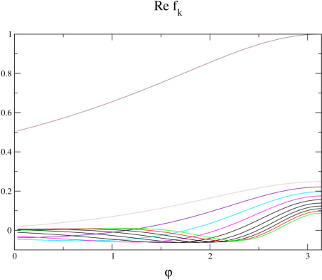
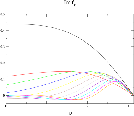
To study the source of the slow convergence of the contour-improved series, it is useful to consider the behavior of the factor , appearing in the integrand of , on the contour . Let , , be any analytic function real on the real axis, and ( thus correspond to timelike and spacelike points, respectively). One then has
| (14) |
The behavior of and as a function of , for and , is shown in Figure 1. We observe that both and have zeroes on the circle , and that these zeroes move with the order . Moreover, while (slowly) decreases with increasing for all angles , the magnitude of is sizeable in the region even for . This slow convergence in the backwards (spacelike) direction is the origin of the slow convergence of the tails of the integrated series shown in Table I, since the factor entering the weight has maximum modulus at the spacelike point on the contour, and is more and more sharply peaked in the backward direction as increases. In addition, the behavior of and happens to be just such that, combined with the changes of sign of the real and imaginary parts of , there is a very strong cancellation in the integral over (particularly so for the case ). This strong cancellation is the origin of the “accidental” suppression of the magnitude of the term. As we have already seen in Table I, it is potentially dangerous to use weights for which the integrals are small for a particular (or for a small number of values of ) only due to such cancellations. Higher order contributions can then easily be large again, thereby spoiling the seemingly good convergence of the first few terms of the contour-improved series.
The behavior of the and displayed in Figure 1 allows one not only to understand the origin of the potential convergence problem but also to construct alternate sum rules which avoid it. From Figure 1 it is evident that convergence can be improved by avoiding weights which are large in the spacelike direction. The results of Ref. [33] also indicate that, for the FESR framework to be reliable at scales , it is necessary for the weight function to have a zero at ().******Such a zero suppresses contributions from the OPE representation in the region near the timelike real axis where, at scales and below, data shows that it breaks down [33]. We have found two approaches useful for implementing these constraints. The first involves the use of polynomials with “shepherd” zeros, i.e., zeros either on, or near, the regions of the contour one wishes to suppress. The second involves the construction of weights, , with peaked on the contour at angles , thereby avoiding large contributions from , (see Figure 1). A convenient and effective choice is to take to have a Gaussian form on the contour. Choosing the width of the Gaussian to be and the center to be , good convergence of the tail of the integrated series can be obtained for any . Technically, these profiles can be well represented using polynomials of degree
| (15) |
The coefficients are determined, upon normalizing such that , by the Fourier integrals
| (16) |
To summarize: given the problems discussed above with those FESR’s involving the spectral weights, , we would like to find, if possible, an alternate weight choice, ,
(1) such that is strongly suppressed in the region above , in order to (a) reduce the degree of cancellation between the and spectral integrals, (b) reduce the impact of the large experimental errors in the spectral distribution above the region, and (c) minimize the role of the longitudinal subtraction which must, at present, be performed theoretically; and
(2) such that emphasizes those regions of the contour for which the convergence of the series is favorable.
It is, of course, not a priori obvious that there exist having the desired properties. We have, however, succeeded in constructing several polynomial weights which do.††††††An important further restriction results from the observation that, in the FESR framework, higher dimension contributions are suppressed only by inverse powers of ; in order to avoid generating potentially large, and unknown, higher dimension contributions, therefore, the coefficients of the polynomials we construct should all be comparable in magnitude to the leading coefficient, . We have chosen to implement this constraint by keeping all coefficients less than in magnitude. Since, as we will see below, the resulting weights do not contain as a factor, the approach is less inclusive than the analysis employing [12, 14], but it has the advantage of being theoretically cleaner.
The strategy involving shepherd zeros can be implemented with the zeros either on or off the contour. The first weight we have constructed satisfying the criteria above has all zeros on the contour, and is given by
| (17) |
The absence of terms, which suppresses contributions, is an additional positive feature of this weight. The fourth order zero at and second order zero at provide the desired suppressions of the timelike and spacelike regions. An alternate family of weights still having a fourth order zero at , but with the remaining zeros moved off the contour and at a distance from the origin, is
| (18) |
( and give the angular positions of the pairs of off-contour complex conjugate zeros corresponding to the last two factors, with respect to the spacelike direction). The choice produces a second solution to the constraints above, one whose biggest coefficient is . We denote this solution by
| (19) |
In the approach based on weights which have imaginary parts with a Gaussian profile on the contour, we choose a basis of such weights having different centers, . As noted above, so long as all the lie in the interval , all of the corresponding integrated perturbative series will be under control. We then form linear combinations of these weights having different in such a way as to construct a new weight which not only retains this good convergence, but at the same time has a zero of sufficiently high order at to strongly suppress contributions to the spectral integral from the region . The weight of this type which most successfully satisfies the criteria discussed above has a rapid high- falloff produced by a order zero at , a largest coefficient , and is given by
| (22) | |||||
The (vastly) improved convergence of the tail of the integrated series for the weights , and is displayed in Table II. The entries, as in Table I, have been rescaled by the corresponding value, and hence correspond to the ratios, . The results also show that an estimate of the truncation error given by the magnitude of the term is, for the new weights, almost certainly a very conservative one. We will demonstrate, in the next section, that the suppression of the high- region of the spectrum produced by the new weights is also sufficient to significantly reduce the impact of the experimental errors.
IV Numerical Analysis and Results
In performing the numerical analysis of the FESR’s constructed above, we employ the ALEPH data for the nonstrange and strange number distributions‡‡‡‡‡‡The 1998 tabulation of the nonstrange data receives a small overall normalization correction as a result of the shift in between the preliminary 1998 and final 1999 analyses. We thank Shaomin Chen for bringing this point to our attention. and PDG98 values for , , and . As noted above, the weights have been chosen in such a way that, although theoretical input is required in order to subtract the longitudinal contributions to the experimental number distributions, and hence obtain the spectral functions, the effect of this subtraction on the final value of is negligible. We will quantify this statement below. Once the spectral function has been determined, it is a straightforward matter to evaluate the weighted spectral integrals. The choice of steeply falling weights ensures that the strange spectral integrals are dominated by the and contributions, for which the experimental errors are much smaller than those of the rest of the strange number distribution. This plays a major role in reducing the impact of experimental errors on the final extracted value of . To get a realistic determination of these errors it is important to separate correlated and uncorrelated errors, and also to take into account the strong correlations between the spectral integrals involving different weights.
The nature of the longitudinal subtraction differs significantly in the low- and high- () regions. For low , the and pole subtractions are experimentally unambiguous. For high (the resonance region), the longitudinal contributions are proportional to , , for , , respectively, and hence dominated by the contributions. The longitudinal vector contribution is inferred from the strange scalar spectral function of Ref. [5]. This procedure is consistent provided the value of resulting from the present analysis is compatible with that from the strange scalar channel [9], which it turns out to be. The longitudinal axial vector contribution is similarly inferred from the spectral function of the strange pseudoscalar channel. The latter is obtained by fixing the excited resonance decay constants of a sum-of-resonances spectral ansatz through matching of the hadronic and OPE sides of a family of “pinch-weighted” FESR’s, in analogy to the analysis of Ref [34].******The corresponding procedure works very well in the isovector vector channel, where the results can be checked against the well-known experimental spectral function [34]. A similar statement is true even in channels with strongly attractive interactions near threshold, for which the spectral function will be poorly represented near threshold by the tail of a Breit-Wigner resonance form with “conventional” -dependent width. For example, using the value of obtained from the strange scalar channel analysis as input and redoing the strange scalar channel analysis, using now a sum-of-resonances spectral ansatz in place of the more realistic ansatz of Ref. [5], one finds that the ansatz of Ref. [5] is well-reproduced in the region of the dominant peak. One can also use this approach to check the self-consistency between the assumed longitudinal contributions and the output value in kinematic-weight-based analysis of Ref. [13, 15]. It turns out that the high- longitudinal contributions assumed are more than a factor of smaller than would be expected based on the extracted value of . If one employs the PDG98 values for and , as discussed above, however, the assumed longitudinal contribution becomes compatible within the errors assigned to it in Ref. [13, 15]. The input value of required for this analysis should, in principle, be determined iteratively. We have, however, employed as input the value of obtained from the strange scalar analysis of Ref. [9], . This turns out to be consistent with our final result for . Moreover, for the steeply-falling weights employed in our analysis, the sum of the high- and longitudinal subtractions is at the level of the spectral integral, and hence at the level in the - difference. As such, even were our evaluation to be in error by , the effect on would be completely negligible on the scale of the other errors present in the analysis.
On the OPE side, we retain contributions up to and including . The leading term was given above.
| (24) | |||||
where is the usual RG invariant modification of the non-normal-order strange quark condensate [35], is the average of the light , masses, and is the light () condensate. We use the quark mass ratios determined from the ChPT analyses of Ref. [36], the GMO relation , and the range of values [2, 3] for the ratio of condensates. The contour integrals are performed as described below.
For the contribution we employ a rescaled version of the vacuum saturation approximation (VSA). From the results of Ref. [29], one finds
| (25) |
where represents a multiplicative rescaling of the VSA estimate. The analogous rescaling has been determined empirically for the isovector vector channel and the isospin-breaking vector correlator, and found to be in both cases [37, 22]. For the weights employed in our analysis, it turns out that the integrated contributions are very small. We are, therefore, able to employ the very conservative estimate for the degree of VSA violation without significantly affecting the overall theoretical error. The combination in Eq. (25) is to be understood as an effective RG-invariant combination for the evaluation of the OPE contour integrals.
Finally, for the contribution, we assume
| (26) |
For this term does not contribute to the integrated OPE; for and , the value of the effective RG-invariant condensate combination, , is to be determined as part of the analysis.
As noted above, the OPE contour integrals (for all ) are performed using the contour improvement prescription. Four-loop versions of the running mass and coupling are employed. To be specific, we have solved analytically for the running mass and coupling using the 4-loop truncated versions of the [38] and [39] functions, with the value determined in nonstrange hadronic decays, [23], as input. Following conventional practice, we take the error associated with the truncation of the perturbative series for the Wilson coefficient of the term at to be equal to the value of the last () contribution retained. In light of the discussion above we consider this to represent an extremely conservative estimate.
From the point of view of uncertainties on the OPE side, the sum rule is favored over the and sum rules for three reasons: (1) it has no contributions, (2) it has the smallest truncation error, and (3) it has the smallest errors associated with uncertainties in the input values of the and condensates.*†*†*†Combining the errors associated with truncation, the condensate input values, and the uncertainty on in quadrature, the resulting errors on are , and for , and , respectively. In Table III we display, as a function of , the extracted values of obtained from the sum rule, analyzed neglecting contributions of dimension 12 and higher. Central values have been used for all input on the OPE side and for the experimental spectral data. For the analysis to be self-consistent, the extracted value of should be independent of . This will be true for sufficiently large that the contributions are negligible. As is decreased, the extracted values should eventually deviate from a constant, signalling the growth of the higher dimension terms. From the Table we see that the range provides an extremely good window of stability. In view of the falloff begining around , we will work in the range in the discussions which follow. It is worth stressing that the central values obtained from and sum rules, though having slightly larger theoretical errors, are nonetheless completely consistent with those above: in the window , one finds that the range of solutions for lies between and for , and for , and, as we saw already in Table III, and for . In contrast, the sum rule, for which the longitudinal subtraction is important, and the convergence is not well under control, yields a range between and (with, moreover, inconsistent solutions for ).
From the point of view of the impact of the errors present in existing experimental data, the theoretically favored weight is, unfortunately, no longer the favored one. The reason is that, although the impact of the errors in the high- region of the spectrum has been strongly suppressed by the rapid falloff of the weights employed, the - cancellation is still rather close (e.g., at , to the level of for , for and for , to be compared with , and for the , .) Although the dominant errors (those from the region of the spectrum) are reasonably small, they are still large enough that the relative size of the residual statistical error grows very rapidly with the increase in the degree of cancellation. Thus, e.g., at , the statistical error represents , , , , and of the - spectral difference for the , , , , , and sum rules, respectively.*‡*‡*‡Because of the high degree of cancellation, reducing , which increases the degree of suppression of the (already small) high- contributions, still has a non-trivial effect; e.g., the relative statistical error for the sum rule is reduced from to when is lowered from to . The present experimental situation is, therefore, such that the errors on our final result for are minimized by working with , rather than .
Working with the sum rule in the window specified above we find, for our best fit,
| (27) |
which is equivalent to
| (28) |
where in both of Eqs. (27) and (28) the first error is statistical, the second is due to the uncertainty on , and the third theoretical. The theoretical error has been obtained by combining the following in quadrature (where we quote the numerical values corresponding to Eq. (27) to be specific): , associated with the error on ; , associated with the uncertainty in ; , associated with the variation of within the window ; , associated with the uncertainty in the VSA-violating parameter, ; and , associated with truncation of the series. The latter obviously remains the dominant source of theoretical error, despite the significant improvement produced by the use of the new weights. Figure 2 displays the quality of the match between the OPE and spectral integral sides of the sum rule corresponding to the fit above; the agreement in the previously-established stability window, , is obviously excellent. The divergence of the OPE and spectral integral curves below is precisely what one would expect based on the observation above that, for the sum rule, contributions, not included in the truncated OPE representation, begin to become important in this region.
The result of Eqs. (27) and (28) is in good agreement with the strange scalar channel results of Refs. [5] and [9], the strange pseudoscalar channel result of Ref. [8], and the recent hadronic decay analysis of Ref. [14], but, we believe, has signficantly reduced theoretical and experimental errors. In particular, the statistical error has, at this point, been reduced almost to the level of that associated with the uncertainty in .
Improvements in the accuracy of the experimental spectral data, in particular in the region, could lead to a significant improvement in the size of the statistical error. Such an improvement should be possible using BaBar data[40]. Reduced uncertainties in our knowledge of would also be helpful. On the theoretical side, while significant improvements in the accuracy of the spectral data would allow one to move from the to the sum rule, the decrease in the theoretical uncertainty that would result from this shift would be only . Far more likely to lead to a significant improvement in the size of the theoretical error would be a computation of the coefficient in the contribution to the flavor-breaking correlator difference, .
ACKNOWLEDGMENTS
The authors would like to thank A. Höcker and S. Chen for providing detailed information on the ALEPH nonstrange and strange spectral distributions, S. Chen for pointing out the normalization correction to the 1998 nonstrange data necessitated by the results of the 1999 strange data analysis, and G. Colangelo for his collaboration at an early stage of this work. KM acknowledges the ongoing support of the Natural Sciences and Engineering Research Council of Canada, and the hospitality of the Special Research Centre for the Subatomic Structure of Matter at the University of Adelaide, where much of this work was performed, and JK the partial support of the Schweizerischer Nationalfonds and the EEC-TMR program, Contract No. CT 98-0169.
| Weight | |||||||||||
|---|---|---|---|---|---|---|---|---|---|---|---|
| 1 | 0.143 | -0.007 | -0.145 | -0.237 | -0.286 | -0.294 | -0.272 | -0.233 | -0.187 | -0.141 | |
| 1 | 0.209 | 0.100 | -0.027 | -0.143 | -0.232 | -0.287 | -0.308 | -0.300 | -0.272 | -0.233 | |
| 1 | 0.257 | 0.187 | 0.076 | -0.048 | -0.143 | -0.260 | -0.324 | -0.357 | -0.359 | -0.339 |
| Weight | |||||||||||
|---|---|---|---|---|---|---|---|---|---|---|---|
| 1 | 0.262 | 0.213 | 0.143 | 0.073 | 0.018 | -0.017 | -0.033 | -0.034 | -0.027 | -0.016 | |
| 1 | 0.232 | 0.165 | 0.092 | 0.032 | -0.008 | -0.030 | -0.038 | -0.038 | -0.035 | -0.032 | |
| 1 | 0.248 | 0.193 | 0.125 | 0.064 | 0.019 | -0.009 | -0.023 | -0.026 | -0.024 | -0.020 |
| (GeV2): | 2.35 | 2.55 | 2.75 | 2.95 | 3.15 |
|---|---|---|---|---|---|
| (MeV): | 153.2 | 159.0 | 162.2 | 163.4 | 163.2 |

REFERENCES
- [1] J. Bijnens, J. Prades and E. de Rafael, Phys. Lett. B348, 226 (1995).
- [2] M. Jamin and M. Münz, Z. Phys. C66, 633 (1995); M. Jamin, Nucl. Phys. B (Proc. Suppl.) 64, 250 (1998).
- [3] K.G. Chetyrkin, D. Pirjol and K. Schilcher, Phys. Lett. B404, 337 (1997).
- [4] S. Narison, Phys. Lett. B358, 113 (1995).
- [5] P. Colangelo, F. De Fazio, G. Nardulli and N. Paver, Phys. Lett. B408, 340 (1997).
- [6] T. Bhattacharya, R. Gupta and K. Maltman, Phys. Rev. D57, 5455 (1998).
- [7] K. Maltman, Phys. Lett. B428, 179 (1998).
- [8] C. Dominguez, L. Pirovano and K. Schilcher, Phys. Lett. B425, 193 (1998).
- [9] K. Maltman, Phys. Lett. B462, 195 (1999).
- [10] K.G. Chetyrkin and A. Kwiatkowski, Z. Phys. C59, 525 (1993) and hep-ph/9805232.
- [11] K. Maltman, Phys. Rev. D58: 093015 (1998).
- [12] A. Pich and J. Prades, JHEP 9806:013 (1998).
- [13] S. Chen, M. Davier and A. Hocker, LAL-98-90, Nov. 1998.
- [14] A. Pich and J. Prades, JHEP 9910:004 (1999).
- [15] The ALEPH Collaboration, Eur. Phys. J. C11, 599 (1999), hep-ex/9903015.
- [16] S. Narison, Phys. Lett. B466, 345 (1999); hep-ph/9905264.
- [17] S. Narison, Nucl. Phys. Proc. Suppl. 86, 242 (2000), hep-ph/9911454.
- [18] R. Gupta and T. Bhattacharya, Phys. Rev. D55, 7203 (1997) and Nucl. Phys. (Proc. Suppl.) 63, 45 (1998); B.J. Gough et al., Phys. Rev. Lett. 79, 1662 (1997).
- [19] R.D. Kenway, Nucl. Phys. (Proc. Suppl.) 73, 16 (1999).
- [20] V. Lubicz, Nucl. Phys. (Proc. Suppl.) 74, 291 (1999).
- [21] T. Blum, A. Soni and M. Wingate, Phys. Rev. D60: 114507 (1999); J. Gardner, J. Heitger, R. Sommer and H. Wettig (ALPHA/UKQCD), Nucl. Phys. B571, 237 (2000); S. Aoki, et al. (JLQCD), Phys. Rev. Lett. 82, 4392 (1999); S. Aoki et al. (CP-PACS), Phys. Rev. Lett. 84, 238 (2000); W. Göckeler et al. (QCDSF), hep-lat/9908005; D. Becirevic, V. Lubicz, G. Martinelli and M. Testa, hep-lat/9909039; A. Ali Khan, et al. (CP-PACS), hep-lat/9909050 and hep-lat/0004010.
- [22] K. Maltman and C.E. Wolfe, Phys. Rev. D59: 096003 (1999).
- [23] R. Barate et al. (The ALEPH Collaboration), Z. Phys. C76, 379 (1997); Eur. Phys. J. C4, 409 (1998).
- [24] E. Golowich and J. Kambor, Phys. Rev. D53, 2651 (1996).
- [25] S. Dürr and J. Kambor, Phys. Rev. D61: 114025 (2000).
- [26] Review of Particle Properties, Eur. Phys. J. C3, 1 (1998).
- [27] Y.S. Tsai, Phys. Rev. D4, 2821 (1971); H.B. Thacker and J.J. Sakurai, Phys. Lett. B36, 103 (1971); F.J. Gilman and D.H. Miller, Phys. Rev. D17, 1846 (1978); F.J. Gilman and S.H. Rhie, Phys. Rev. D31, 1066 (1985).
- [28] E. Braaten, Phys. Rev. Lett. 60, 1606 (1988); S. Narison and A. Pich, Phys. Lett. B211, 183 (1988); E. Braaten, Phys. Rev. D39, 1458 (1989); S. Narison and A. Pich, Phys. Lett. B304, 359 (1993).
- [29] E. Braaten, S. Narison and A. Pich, Nucl. Phys. B373, 581 (1992).
- [30] A.A. Pivovarov, Sov. J. Nucl. Phys. 54, 676 (1991) and Z. Phys. C53, 461 (1992); F. Le Diberder and A. Pich, Phys. Lett. B286, 147 (1992) and B289, 165 (1992).
- [31] A. Pich, hep-ph/9704453, in “Heavy Flavors II”, eds. A.J. Buras and M. Lindner, World Scientific, 1997.
- [32] W.J. Marciano and A. Sirlin, Phys. Rev. Lett. 61, 1815 (1988).
- [33] K. Maltman, Phys. Lett. B440, 367 (1998).
- [34] K. Maltman, Phys. Lett. B462, 14 (1999).
- [35] K. Chetyrkin and K.G. Spiridonov, Sov. J. Nucl. Phys. 47, 3 (1988).
- [36] H. Leutwyler, Phys. Lett. B374, 163 (1996); Phys. Lett. B378, 313 (1996) and hep-ph/9609467.
- [37] S. Narison, Phys. Lett. B361, 121 (1995).
- [38] T. van Ritbergen, J.A.M. Vermaseren and S.A. Larin, Phys. Lett. B400, 379 (1997).
- [39] K.G. Chetyrkin, Phys. Lett. B404, 161 (1997); T. Van Ritbergen, J.A.M. Vermaseren and S.A. Larin, Phys. Lett. B405, 327 (1997).
- [40] M. Roney, private communication.