The double parton distributions in the hard pomeron model

Mikhail  Braun Department of High-Energy Physics, University of St. Petersburg, 198904 St.Petersburg, Russia    Daniele  Treleani Department of Theoretical Physics, University of Trieste, Strada Costiera 11, Istituto Nazionale di Fisica Nucleare, Sezione di Trieste, and ICTP, I–34014, Trieste,Italy

Abstract.

We study the double parton interaction process in collisions between highly virtual qq¯𝑞¯𝑞q{\bar{q}} pairs in the BFKL regime. Explicit expressions for the double parton distributions are obtained both in the case of direct coupling of the BFKL pomerons to the qq¯𝑞¯𝑞q{\bar{q}} pair and in the case of triple pomeron interaction.

E-mail braun1@MB1693.spb.edu

E-mail daniel@trieste.infn.it

I Introduction.

An important feature of hadronic collisions at high energies is the growth of the hard component of the interaction, induced by the increasing flux of partons. Apart from the single hard interaction, multi-parton hard interactions begin to play an increasing role. Hard events with multi-parton interactions have in fact been predicted long ago by several authors[1]. The simplest event of this kind, the double parton scattering, has been an object of the experimental search in all high energy hadron collider experiments since several years[2] and while initially the results have been sparse and not very consistent, recently CDF has reported the observation of a large number of events with double parton collisions[3].

Multiple parton collisions represent a new observable feature of hadronic interactions. Non-perturbative inputs to the corresponding cross sections are the multi-parton distributions. These are new properties of the hadron structure which become accessible through the observation of multiple parton collisions. The multiple parton distributions are related directly to the many-body parton correlations in the hadron[4]. While, as a general rule, the non-perturbative inputs are quantities to be measured and which cannot be computed in perturbation theory, in the interaction of two very virtual qq¯𝑞¯𝑞q{\bar{q}} pairs, the whole process falls in the domain of perturbative QCD and, in that case, multiple parton distributions can be obtained through a direct calculation, within an approximation scheme. The aim of the present paper is to study precisely this example of high energy interaction and to work out explicitly the simplest case of multi-parton distribution.

Note that studying events with several hard interactions one can introduce standard notions of inclusive and exclusive cross-sections. The first refer to the observation of at least one (or two,..) hard events, the second of exactly one (or two,…) hard events. The inclusive hard cross-sections are most easily accessable in the experimental study. They are also most easily calculated theoretically. In fact the inclusive cross sections are basically average quantities, since they include the multiplicity factor, which is proportional to the number of hard partonic interactions[5], so no wonder that the inclusive cross-section may become larger than the total cross-section [6]. The AGK rules[7] tell that the inclusive cross-sections for single, double, triple etc hard collisions are given by the simplest relevant diagrams, which involve one, two, three etc hard interaction blobs. All other contributions from diagrams with more hard blobs cancel in the inclusive cross-sections. In the following, applying the simple theoretical formulas for the inclusive cross-sections, we shall use them as basic quantities, from which we shall extract the multiparton distributions.

The paper is organized in two parts. For the sake of completeness the kinematics of the single and double parton collision and the factorization of the non-perturbative parts of the processes are re-derived in the first part of the paper. In the second part, using the perturbative QCD approach, we compute the double parton distribution in two different limiting cases. The last paragraph is devoted to the conclusions.

II Single and double parton interactions

A Single hard scattering

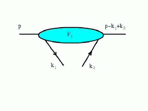
To fix our notations and to settle a common ground with the double parton collision process, we discuss first the single hard scattering case which is described by the diagram shown in Fig.1. The discontinuity of the diagram through the hard blob represents the inclusive cross section and, because of the AGK cancellation[7], it includes the factor accounting for the multiplicity of the hard partonic collisions in the hadronic interaction[5]. In the following one considers only one sort of partons which, for the hard pomeron model, is represented by the gluons. The contribution of the diagram to the inclusive cross-section is related to the amplitude by

σ=(1/s)Im𝒜𝜎1𝑠Im𝒜\sigma=(1/s){\rm Im}{\cal A} (1)

where s=2p+q𝑠2subscript𝑝subscript𝑞s=2p_{+}q_{-} is the c.m energy squared. We neglect the masses of the projectile and target and take p=q+=p=q=0subscript𝑝subscript𝑞subscript𝑝perpendicular-tosubscript𝑞perpendicular-to0p_{-}=q_{+}=p_{\perp}=q_{\perp}=0. For massive projectile and target the standard substitution ppαq𝑝𝑝𝛼𝑞p\rightarrow p-\alpha q, qqαp𝑞𝑞𝛼𝑝q\rightarrow q-\alpha p with α=m2/s𝛼superscript𝑚2𝑠\alpha=m^{2}/s is assumed. The usual scaling variables of the colliding partons are introduces as

k+=xp+,l=wqformulae-sequencesubscript𝑘𝑥subscript𝑝subscript𝑙𝑤subscript𝑞k_{+}=xp_{+},\ \ l_{-}=wq_{-} (2)

The partonic c.m. energy squared is therefore written as spM2=(k+l)22k+l=sxwsubscript𝑠𝑝superscript𝑀2superscript𝑘𝑙2similar-to-or-equals2subscript𝑘subscript𝑙𝑠𝑥𝑤s_{p}\equiv M^{2}=(k+l)^{2}\simeq 2k_{+}l_{-}=sxw.

The standard treatment is based on two assumptions which are the basis for the factorization hypothesis

* Parton virtualities (essentially the transverse momenta squared) are much smaller as compared with M2superscript𝑀2M^{2}.

** The dependence of the forward amplitude a𝑎a on the virtualities of the external lines can be neglected.

The longitudinal integrations in the diagram of Fig.1 are easily done. Indeed according to our assumptions the amplitude a𝑎a does not depend on ksubscript𝑘k_{-} nor on l+subscript𝑙l_{+}. Only the upper part of the diagram depends therefore on ksubscript𝑘k_{-}. One denotes it (with parton legs) as F1(p,k)subscript𝐹1𝑝𝑘F_{1}(p,k). Its integration over ksubscript𝑘k_{-} is standardly transformed into the integration over the “missing mass” s1=(pk)2subscript𝑠1superscript𝑝𝑘2s_{1}=(p-k)^{2} of its right-hand discontinuity:

dk2πF1(p,k)=i2p+s10ds1πImF1(p,k)2πixp+F1(x,k)𝑑subscript𝑘2𝜋subscript𝐹1𝑝𝑘𝑖2subscript𝑝superscriptsubscriptsubscript𝑠10𝑑subscript𝑠1𝜋Imsubscript𝐹1𝑝𝑘2𝜋𝑖𝑥subscript𝑝subscript𝐹1𝑥subscript𝑘perpendicular-to\int\frac{dk_{-}}{2\pi}F_{1}(p,k)=\frac{i}{2p_{+}}\int_{s_{10}}^{\infty}\frac{ds_{1}}{\pi}{\rm Im}\,F_{1}(p,k)\equiv\frac{2\pi i}{xp_{+}}F_{1}(x,k_{\perp}) (3)

Similarly for the target

dl+2πF2(q,l)=i2qs20ds2πImF2(q,l)2πiwqF2(w,l)𝑑subscript𝑙2𝜋subscript𝐹2𝑞𝑙𝑖2subscript𝑞superscriptsubscriptsubscript𝑠20𝑑subscript𝑠2𝜋Imsubscript𝐹2𝑞𝑙2𝜋𝑖𝑤subscript𝑞subscript𝐹2𝑤subscript𝑙perpendicular-to\int\frac{dl_{+}}{2\pi}F_{2}(q,l)=\frac{i}{2q_{-}}\int_{s_{20}}^{\infty}\frac{ds_{2}}{\pi}{\rm Im}\,F_{2}(q,l)\equiv\frac{2\pi i}{wq_{-}}F_{2}(w,l_{\perp}) (4)

The standard parton distributions at the scale M2superscript𝑀2M^{2} are obtained by integrating F1subscript𝐹1F_{1} and F2subscript𝐹2F_{2} over the transverse momenta ksubscript𝑘perpendicular-tok_{\perp} and lsubscript𝑙perpendicular-tol_{\perp}:

ρ1(x,M2)=d2k(2π)2θ(M2k2)F1(x,k)subscript𝜌1𝑥superscript𝑀2superscript𝑑2𝑘superscript2𝜋2𝜃superscript𝑀2superscript𝑘2subscript𝐹1𝑥𝑘\rho_{1}(x,M^{2})=\int\frac{d^{2}k}{(2\pi)^{2}}\theta(M^{2}-k^{2})F_{1}(x,k) (5)

The final integrations over k+subscript𝑘k_{+} and lsubscript𝑙l_{-} can be transformed into integrations over x𝑥x and w𝑤w. The integration limits, [0,1]01[0,1], are a consequence of the positivity constraints of s1,s2subscript𝑠1subscript𝑠2s_{1},s_{2} and M2superscript𝑀2M^{2}. The amplitude of Fig. 1 is therefore written as

𝒜1=01dxdwxwρ1(x,M2)ρ2(w,M2)a(M2)subscript𝒜1superscriptsubscript01𝑑𝑥𝑑𝑤𝑥𝑤subscript𝜌1𝑥superscript𝑀2subscript𝜌2𝑤superscript𝑀2𝑎superscript𝑀2{\cal A}_{1}=\int_{0}^{1}\frac{dxdw}{xw}\rho_{1}(x,M^{2})\rho_{2}(w,M^{2})a(M^{2}) (6)

while the single parton scattering inclusive cross-sections is expressed by the usual factorized formula:

σ1=01𝑑x𝑑wρ1(x,M2)ρ2(w,M2)σp(xw)subscript𝜎1superscriptsubscript01differential-d𝑥differential-d𝑤subscript𝜌1𝑥superscript𝑀2subscript𝜌2𝑤superscript𝑀2subscript𝜎𝑝𝑥𝑤\sigma_{1}=\int_{0}^{1}dxdw\rho_{1}(x,M^{2})\rho_{2}(w,M^{2})\sigma_{p}(xw) (7)

The cross section can be expressed by using the unintegrated parton distributions in coordinate space. To this purpose one introduces the (non-forward) target parton distribution F1(x,k1,k2)subscript𝐹1𝑥subscript𝑘perpendicular-to1absentsubscript𝑘perpendicular-to2absentF_{1}(x,k_{1\perp},k_{2\perp}), shown in Fig.2, and its Fourier transform

F1(x,r1,r2)=d2k1d2k2(2π)4F1(x,k1,k2)eik1r1ik2r2subscript𝐹1𝑥subscript𝑟1subscript𝑟2superscript𝑑2subscript𝑘1superscript𝑑2subscript𝑘2superscript2𝜋4subscript𝐹1𝑥subscript𝑘1subscript𝑘2superscript𝑒𝑖subscript𝑘1subscript𝑟1𝑖subscript𝑘2subscript𝑟2F_{1}(x,r_{1},r_{2})=\int\frac{d^{2}k_{1}d^{2}k_{2}}{(2\pi)^{4}}F_{1}(x,k_{1},k_{2})e^{ik_{1}r_{1}-ik_{2}r_{2}} (8)

(In the following part of this subsection one will not find 4-vectors, so we suppress the subindex perpendicular-to\perp for the k𝑘k’s). It is convenient to introduce the partonic c.m. and relative coordinates by

r1+r2=2R,r1r2=rformulae-sequencesubscript𝑟1subscript𝑟22𝑅subscript𝑟1subscript𝑟2𝑟r_{1}+r_{2}=2R,\ \ r_{1}-r_{2}=r (9)

One has therefore

F1(x,k1,k2)=d2Rd2rF1(x,R,r)eiR(k1k2)ir(k1+k2)/2subscript𝐹1𝑥subscript𝑘1subscript𝑘2superscript𝑑2𝑅superscript𝑑2𝑟subscript𝐹1𝑥𝑅𝑟superscript𝑒𝑖𝑅subscript𝑘1subscript𝑘2𝑖𝑟subscript𝑘1subscript𝑘22F_{1}(x,k_{1},k_{2})=\int d^{2}Rd^{2}rF_{1}(x,R,r)e^{-iR(k_{1}-k_{2})-ir(k_{1}+k_{2})/2} (10)

and when k1subscript𝑘1k_{1} and k2subscript𝑘2k_{2} are equal

F1(x,k)=F1(x,k,k)=d2Rd2rF1(x,R,r)eirksubscript𝐹1𝑥𝑘subscript𝐹1𝑥𝑘𝑘superscript𝑑2𝑅superscript𝑑2𝑟subscript𝐹1𝑥𝑅𝑟superscript𝑒𝑖𝑟𝑘F_{1}(x,k)=F_{1}(x,k,k)=\int d^{2}Rd^{2}rF_{1}(x,R,r)e^{-irk} (11)

which is precisely the unintegrated parton distribution which appeared in the single hard scattering expression above. According to (5) one has to integrate F1subscript𝐹1F_{1} over all k𝑘k values, with the condition k2<<M2much-less-thansuperscript𝑘2superscript𝑀2k^{2}<<M^{2}, in order to obtain the final partonic distribution at the scale M2superscript𝑀2M^{2}. In the scaling approximation the ρ𝜌\rho’s do not depend on M2superscript𝑀2M^{2}. One may therefore take the limit M2superscript𝑀2M^{2}\rightarrow\infty and thus integrate over all k𝑘k-values. In the scaling approximation one therefore finds

ρ1(x,M2)=d2RF1(x,R,0)subscript𝜌1𝑥superscript𝑀2superscript𝑑2𝑅subscript𝐹1𝑥𝑅0\rho_{1}(x,M^{2}\rightarrow\infty)=\int d^{2}RF_{1}(x,R,0) (12)

When keeping into account the limits for k2superscript𝑘2k^{2} the value r=0𝑟0r=0 is changed into r21/M2similar-to-or-equalssuperscript𝑟21superscript𝑀2r^{2}\simeq 1/M^{2}. The standard parton distributions ρ(x,M2)𝜌𝑥superscript𝑀2\rho(x,M^{2}), entering in the factorization formula, can be therefore expressed via the density in coordinate space F𝐹F as

ρ(x,M2)=d2RF(x,R,r),r2=1/M2formulae-sequence𝜌𝑥superscript𝑀2superscript𝑑2𝑅𝐹𝑥𝑅𝑟superscript𝑟21superscript𝑀2\rho(x,M^{2})=\int d^{2}RF(x,R,r),\ \ r^{2}=1/M^{2} (13)

B Double hard scattering

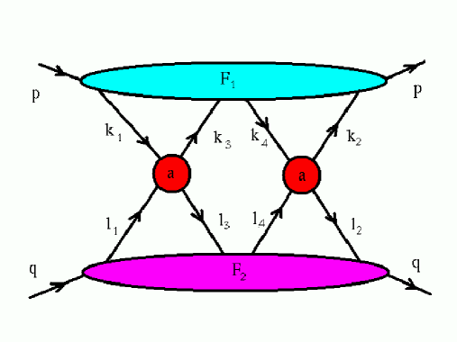
The double hard scattering diagram is shown in Fig.3. The corresponding inclusive cross section (including the multiplicity factor) is obtained, by means of the AGK rules[7], by taking twice the imaginary part and dividing it by s𝑠-s.

The previous analysis can be repeated also in this case. There are five double longitudinal integrations. As independent variables one chooses k1,k2,l1,l2subscript𝑘1subscript𝑘2subscript𝑙1subscript𝑙2k_{1},k_{2},l_{1},l_{2} and q=k1k3𝑞subscript𝑘1subscript𝑘3q=k_{1}-k_{3}. The two hard scattering amplitudes are assumed to depend only on their total c.m. energies squared M12=(k1+l1)2=2k1+l1superscriptsubscript𝑀12superscriptsubscript𝑘1subscript𝑙122subscript𝑘limit-from1subscript𝑙limit-from1M_{1}^{2}=(k_{1}+l_{1})^{2}=2k_{1+}l_{1-} and M22=(k2+l2)2=2k2+l2superscriptsubscript𝑀22superscriptsubscript𝑘2subscript𝑙222subscript𝑘limit-from2subscript𝑙limit-from2M_{2}^{2}=(k_{2}+l_{2})^{2}=2k_{2+}l_{2-}, not on k1(2)subscript𝑘limit-from12k_{1(2)-}, l1(2)+subscript𝑙limit-from12l_{1(2)+} nor on q±subscript𝑞plus-or-minusq_{\pm}. The integrations on k1(2)subscript𝑘limit-from12k_{1(2)-} are made as in the single scattering case. One calls the projectile blob (with all four partonic legs) F1(p,k1,k2,k3,k4)subscript𝐹1𝑝subscript𝑘1subscript𝑘2subscript𝑘3subscript𝑘4F_{1}(p,k_{1},k_{2},k_{3},k_{4}) (ki=0subscript𝑘𝑖0\sum k_{i}=0). Then the integrations over k1(2)subscript𝑘limit-from12k_{1(2)-} can be transformed into integrations over the missing masses of the two hard scatterings s1=(pk1)2subscript𝑠1superscript𝑝subscript𝑘12s_{1}=(p-k_{1})^{2} and s2=(pk2)2subscript𝑠2superscript𝑝subscript𝑘22s_{2}=(p-k_{2})^{2}, the integrand being the discontinuity of F𝐹F on the corresponding right-hand cuts.

Since neither the hard scattering amplitudes nor F2subscript𝐹2F_{2} depend on qsubscript𝑞q_{-} one may integrate F1subscript𝐹1F_{1} also over qsubscript𝑞q_{-}. This last integration can be transformed into an integration over the missing mass in between the scatterings s3=(pq)2subscript𝑠3superscript𝑝𝑞2s_{3}=(p-q)^{2} along the right-hand cut, the integrand being the corresponding discontinuity. As a result one obtains


(i2p+)3s10ds12πis20ds22πis30ds32πiDiscs1Discs2Discs3F1(p,k1,k2,k3,k4)superscript𝑖2subscript𝑝3superscriptsubscriptsubscript𝑠10𝑑subscript𝑠12𝜋𝑖superscriptsubscriptsubscript𝑠20𝑑subscript𝑠22𝜋𝑖superscriptsubscriptsubscript𝑠30𝑑subscript𝑠32𝜋𝑖subscriptDiscsubscript𝑠1subscriptDiscsubscript𝑠2subscriptDiscsubscript𝑠3subscript𝐹1𝑝subscript𝑘1subscript𝑘2subscript𝑘3subscript𝑘4\displaystyle\left(\frac{i}{2p_{+}}\right)^{3}\int_{s_{10}}^{\infty}\frac{ds_{1}}{2\pi i}\int_{s_{20}}^{\infty}\frac{ds_{2}}{2\pi i}\int_{s_{30}}^{\infty}\frac{ds_{3}}{2\pi i}{\rm Disc}_{s_{1}}{\rm Disc}_{s_{2}}{\rm Disc}_{s_{3}}F_{1}(p,k_{1},k_{2},k_{3},k_{4})

2π2i(1p+)3F1(x1,k1,k3|x2,k4,,k2)absent2superscript𝜋2𝑖superscript1subscript𝑝3subscript𝐹1subscript𝑥1subscript𝑘perpendicular-to1absentconditionalsubscript𝑘perpendicular-to3absentsubscript𝑥2subscript𝑘4perpendicular-tosubscript𝑘perpendicular-to2absent\equiv-2\pi^{2}i\left(\frac{1}{p_{+}}\right)^{3}F_{1}(x_{1},k_{1\perp},k_{3\perp}|x_{2},k_{4,\perp},k_{2\perp}) (14)

The density defined on the right-hand side is the generalization of the single to the double unintegrated partonic density. The double parton distribution of the target is introduced in an analogous way. The integrations over k1(2)+subscript𝑘limit-from12k_{1(2)+}, l1(2)subscript𝑙limit-from12l_{1(2)-} are transformed into integrations on the scaling variables x1,2subscript𝑥12x_{1,2} and w1,2subscript𝑤12w_{1,2} and the double hard scattering amplitude of Fig.3 is expressed as


𝒜2=i2s01dx1x1dx2x2dw1w1dw2w2j=14d2kj(2π)2d2lj(2π)2(2π)2subscript𝒜2𝑖2𝑠superscriptsubscript01𝑑subscript𝑥1subscript𝑥1𝑑subscript𝑥2subscript𝑥2𝑑subscript𝑤1subscript𝑤1𝑑subscript𝑤2subscript𝑤2superscriptsubscriptproduct𝑗14superscript𝑑2subscript𝑘𝑗superscript2𝜋2superscript𝑑2subscript𝑙𝑗superscript2𝜋2superscript2𝜋2\displaystyle{\cal A}_{2}=\frac{i}{2s}\int_{0}^{1}\frac{dx_{1}}{x_{1}}\frac{dx_{2}}{x_{2}}\frac{dw_{1}}{w_{1}}\frac{dw_{2}}{w_{2}}\int\prod_{j=1}^{4}\frac{d^{2}k_{j}}{(2\pi)^{2}}\frac{d^{2}l_{j}}{(2\pi)^{2}}(2\pi)^{2}


δ2(k1k2k3+k4)(2π)2δ2(k1+l1k3l3)(2π)2δ2(k2+l2k4l4)superscript𝛿2subscript𝑘1subscript𝑘2subscript𝑘3subscript𝑘4superscript2𝜋2superscript𝛿2subscript𝑘1subscript𝑙1subscript𝑘3subscript𝑙3superscript2𝜋2superscript𝛿2subscript𝑘2subscript𝑙2subscript𝑘4subscript𝑙4\displaystyle\delta^{2}(k_{1}-k_{2}-k_{3}+k_{4})(2\pi)^{2}\delta^{2}(k_{1}+l_{1}-k_{3}-l_{3})(2\pi)^{2}\delta^{2}(k_{2}+l_{2}-k_{4}-l_{4})

F1(x1,k1,k3|x2,k4,k2)F2(x2,l1,l3|x2,l4,l2)a(M12)a(M22)subscript𝐹1subscript𝑥1subscript𝑘1conditionalsubscript𝑘3subscript𝑥2subscript𝑘4subscript𝑘2subscript𝐹2subscript𝑥2subscript𝑙1conditionalsubscript𝑙3subscript𝑥2subscript𝑙4subscript𝑙2𝑎superscriptsubscript𝑀12𝑎superscriptsubscript𝑀22F_{1}(x_{1},k_{1},k_{3}|x_{2},k_{4},k_{2})F_{2}(x_{2},l_{1},l_{3}|x_{2},l_{4},l_{2})a(M_{1}^{2})a(M_{2}^{2}) (15)

where M12=sx1w1superscriptsubscript𝑀12𝑠subscript𝑥1subscript𝑤1M_{1}^{2}=sx_{1}w_{1} and M22=sx2w2superscriptsubscript𝑀22𝑠subscript𝑥2subscript𝑤2M_{2}^{2}=sx_{2}w_{2}. The double hard scattering cross section is therefore written as


σ2=01𝑑x1𝑑x2𝑑w1𝑑w2j=14d2kj(2π)2d2lj(2π)2subscript𝜎2superscriptsubscript01differential-dsubscript𝑥1differential-dsubscript𝑥2differential-dsubscript𝑤1differential-dsubscript𝑤2superscriptsubscriptproduct𝑗14superscript𝑑2subscript𝑘𝑗superscript2𝜋2superscript𝑑2subscript𝑙𝑗superscript2𝜋2\displaystyle\sigma_{2}=\int_{0}^{1}dx_{1}dx_{2}dw_{1}dw_{2}\int\prod_{j=1}^{4}\frac{d^{2}k_{j}}{(2\pi)^{2}}\frac{d^{2}l_{j}}{(2\pi)^{2}}


(2π)2δ2(k1k2k3+k4)(2π)2δ2(k1+l1k3l3)(2π)2δ2(k2+l2k4l4)superscript2𝜋2superscript𝛿2subscript𝑘1subscript𝑘2subscript𝑘3subscript𝑘4superscript2𝜋2superscript𝛿2subscript𝑘1subscript𝑙1subscript𝑘3subscript𝑙3superscript2𝜋2superscript𝛿2subscript𝑘2subscript𝑙2subscript𝑘4subscript𝑙4\displaystyle(2\pi)^{2}\delta^{2}(k_{1}-k_{2}-k_{3}+k_{4})(2\pi)^{2}\delta^{2}(k_{1}+l_{1}-k_{3}-l_{3})(2\pi)^{2}\delta^{2}(k_{2}+l_{2}-k_{4}-l_{4})

F1(x1,k1,k3|x2,k4,k2)F2(w1,l1,l3|w2,l4,l2)σp(x1w1)σp(x2w2)subscript𝐹1subscript𝑥1subscript𝑘1conditionalsubscript𝑘3subscript𝑥2subscript𝑘4subscript𝑘2subscript𝐹2subscript𝑤1subscript𝑙1conditionalsubscript𝑙3subscript𝑤2subscript𝑙4subscript𝑙2subscript𝜎𝑝subscript𝑥1subscript𝑤1subscript𝜎𝑝subscript𝑥2subscript𝑤2F_{1}(x_{1},k_{1},k_{3}|x_{2},k_{4},k_{2})F_{2}(w_{1},l_{1},l_{3}|w_{2},l_{4},l_{2})\sigma_{p}(x_{1}w_{1})\sigma_{p}(x_{2}w_{2}) (16)

and both in Eq.(15) and in Eq.(16) the integrations are done with the limits k12,k32<M12superscriptsubscript𝑘12superscriptsubscript𝑘32superscriptsubscript𝑀12k_{1}^{2},k_{3}^{2}<M_{1}^{2} and k22,k42<M22superscriptsubscript𝑘22superscriptsubscript𝑘42superscriptsubscript𝑀22k_{2}^{2},k_{4}^{2}<M_{2}^{2}.

The integrations over the transverse components of the transferred momenta are more conveniently performed by going to coordinates space. One introduces therefore

F1(x1,r1,r3|x2,r4,r2)=j=14dkj(2π)2F1(x1,k1,k3|x2,k4,k2)e(ik1r1ik2r2ik3r3+ik4r4)subscript𝐹1subscript𝑥1subscript𝑟1conditionalsubscript𝑟3subscript𝑥2subscript𝑟4subscript𝑟2superscriptsubscriptproduct𝑗14𝑑subscript𝑘𝑗superscript2𝜋2subscript𝐹1subscript𝑥1subscript𝑘1conditionalsubscript𝑘3subscript𝑥2subscript𝑘4subscript𝑘2superscript𝑒𝑖subscript𝑘1subscript𝑟1𝑖subscript𝑘2subscript𝑟2𝑖subscript𝑘3subscript𝑟3𝑖subscript𝑘4subscript𝑟4F_{1}(x_{1},r_{1},r_{3}|x_{2},r_{4},r_{2})=\int\prod_{j=1}^{4}\frac{dk_{j}}{(2\pi)^{2}}F_{1}(x_{1},k_{1},k_{3}|x_{2},k_{4},k_{2})e^{(ik_{1}r_{1}-ik_{2}r_{2}-ik_{3}r_{3}+ik_{4}r_{4})} (17)

where in the integrand all four momenta are independent, in such a way that one is integrating also over the total momentum transferred to the projectile. One introduces the c.m. and relative coordinates defined as:

r1+r3=2R1,r1r3=r13,r4+r2=2R2,r2r4=r24formulae-sequencesubscript𝑟1subscript𝑟32subscript𝑅1formulae-sequencesubscript𝑟1subscript𝑟3subscript𝑟13formulae-sequencesubscript𝑟4subscript𝑟22subscript𝑅2subscript𝑟2subscript𝑟4subscript𝑟24r_{1}+r_{3}=2R_{1},\ \ r_{1}-r_{3}=r_{13},\ \ r_{4}+r_{2}=2R_{2},\ \ r_{2}-r_{4}=r_{24} (18)

so that


r1=R1+r13/2,r3=R1r13/2,r2=R2+r24/2,r4=R2r24/2formulae-sequencesubscript𝑟1subscript𝑅1subscript𝑟132formulae-sequencesubscript𝑟3subscript𝑅1subscript𝑟132formulae-sequencesubscript𝑟2subscript𝑅2subscript𝑟242subscript𝑟4subscript𝑅2subscript𝑟242\displaystyle r_{1}=R_{1}+r_{13}/2,\ \ r_{3}=R_{1}-r_{13}/2,\ \ r_{2}=R_{2}+r_{24}/2,\ \ r_{4}=R_{2}-r_{24}/2

Similar coordinates, with primes, are introduced for the target:


l1+l3=2R1etc.subscript𝑙1subscript𝑙32subscriptsuperscript𝑅1etc\displaystyle l_{1}+l_{3}=2R^{\prime}_{1}\ \ {\rm etc.}

Going to the coordinates space one finds, in Eq.(16), the following exponential


exp{iR1(k1k3)ir13(k1+k3)/2+iR2(k2k4)+ir24(k2+k4)/2\displaystyle\exp\Big{\{}-iR_{1}(k_{1}-k_{3})-ir_{13}(k_{1}+k_{3})/2+iR_{2}(k_{2}-k_{4})+ir_{24}(k_{2}+k_{4})/2


iR1(l1l3)ir13(l1+l3)/2+iR2(l2l4)+ir24(l2+l4)/2}\displaystyle-iR^{\prime}_{1}(l_{1}-l_{3})-ir^{\prime}_{13}(l_{1}+l_{3})/2+iR^{\prime}_{2}(l_{2}-l_{4})+ir^{\prime}_{24}(l_{2}+l_{4})/2\Big{\}}

Also the three δ𝛿\delta functions in Eq.(16) can be represented as integrals over three additional coordinates in transverse space:


(2π)2δ2(k1k2k3+k4)=d2ReiR(k1k2k3+k4)superscript2𝜋2superscript𝛿2subscript𝑘1subscript𝑘2subscript𝑘3subscript𝑘4superscript𝑑2𝑅superscript𝑒𝑖𝑅subscript𝑘1subscript𝑘2subscript𝑘3subscript𝑘4\displaystyle(2\pi)^{2}\delta^{2}(k_{1}-k_{2}-k_{3}+k_{4})=\int d^{2}Re^{iR(k_{1}-k_{2}-k_{3}+k_{4})}


(2π)2δ2(k1+l1k3l3)=d2b1eib1(k1+l1k3l3)superscript2𝜋2superscript𝛿2subscript𝑘1subscript𝑙1subscript𝑘3subscript𝑙3superscript𝑑2subscript𝑏1superscript𝑒𝑖subscript𝑏1subscript𝑘1subscript𝑙1subscript𝑘3subscript𝑙3\displaystyle(2\pi)^{2}\delta^{2}(k_{1}+l_{1}-k_{3}-l_{3})=\int d^{2}b_{1}e^{ib_{1}(k_{1}+l_{1}-k_{3}-l_{3})}


(2π)2δ2(k4+l4k2l2)=d2b2eib2(k4+l4k2l2)superscript2𝜋2superscript𝛿2subscript𝑘4subscript𝑙4subscript𝑘2subscript𝑙2superscript𝑑2subscript𝑏2superscript𝑒𝑖subscript𝑏2subscript𝑘4subscript𝑙4subscript𝑘2subscript𝑙2\displaystyle(2\pi)^{2}\delta^{2}(k_{4}+l_{4}-k_{2}-l_{2})=\int d^{2}b_{2}e^{ib_{2}(k_{4}+l_{4}-k_{2}-l_{2})}

In the scaling limit the integrations over the eight momenta kj,ljsubscript𝑘𝑗subscript𝑙𝑗k_{j},l_{j}, j=1,4𝑗14j=1,...4 produce eight δ𝛿\delta functions:


δ2(R+b1R1r13),δ2(Rb2+R2+r24),δ2(Rb1+R1r13),superscript𝛿2𝑅subscript𝑏1subscript𝑅1subscript𝑟13superscript𝛿2𝑅subscript𝑏2subscript𝑅2subscript𝑟24superscript𝛿2𝑅subscript𝑏1subscript𝑅1subscript𝑟13\displaystyle\delta^{2}(R+b_{1}-R_{1}-r_{13}),\ \ \delta^{2}(-R-b_{2}+R_{2}+r_{24}),\ \ \delta^{2}(-R-b_{1}+R_{1}-r_{13}),


δ2(R+b2R2+r24),δ2(b1R1r13),δ2(b2+R2+r24),superscript𝛿2𝑅subscript𝑏2subscript𝑅2subscript𝑟24superscript𝛿2subscript𝑏1subscriptsuperscript𝑅1subscriptsuperscript𝑟13superscript𝛿2subscript𝑏2subscriptsuperscript𝑅2subscriptsuperscript𝑟24\displaystyle\delta^{2}(R+b_{2}-R_{2}+r_{24}),\ \ \delta^{2}(b_{1}-R^{\prime}_{1}-r^{\prime}_{13}),\ \ \delta^{2}(-b_{2}+R^{\prime}_{2}+r^{\prime}_{24}),


δ2(b1+R1r13),δ2(b2R2+r24)superscript𝛿2subscript𝑏1subscriptsuperscript𝑅1subscriptsuperscript𝑟13superscript𝛿2subscript𝑏2subscriptsuperscript𝑅2subscriptsuperscript𝑟24\displaystyle\delta^{2}(-b_{1}+R^{\prime}_{1}-r^{\prime}_{13}),\ \ \delta^{2}(b_{2}-R^{\prime}_{2}+r^{\prime}_{24})

The integrations over the transverse coordinates give then r13=r13=r24=r24=0subscript𝑟13subscriptsuperscript𝑟13subscript𝑟24subscriptsuperscript𝑟240r_{13}=r^{\prime}_{13}=r_{24}=r^{\prime}_{24}=0, R1=b1subscriptsuperscript𝑅1subscript𝑏1R^{\prime}_{1}=b_{1}, R2=b2subscriptsuperscript𝑅2subscript𝑏2R^{\prime}_{2}=b_{2}, R1=R+b1subscript𝑅1𝑅subscript𝑏1R_{1}=R+b_{1}, R2=R+b2subscript𝑅2𝑅subscript𝑏2R_{2}=R+b_{2}. As a result the double hard cross-section is expressed as an integral over the three impact parameters, R,b1𝑅subscript𝑏1R,b_{1} and b2subscript𝑏2b_{2}


σ2=01𝑑x1𝑑x2𝑑w1𝑑w2σp(x1w1)σp(x2w2)subscript𝜎2superscriptsubscript01differential-dsubscript𝑥1differential-dsubscript𝑥2differential-dsubscript𝑤1differential-dsubscript𝑤2subscript𝜎𝑝subscript𝑥1subscript𝑤1subscript𝜎𝑝subscript𝑥2subscript𝑤2\displaystyle\sigma_{2}=\int_{0}^{1}dx_{1}dx_{2}dw_{1}dw_{2}\sigma_{p}(x_{1}w_{1})\sigma_{p}(x_{2}w_{2})

d2Rd2b1d2b2F1(x1,R+b1,0|x2,R+b2,0)F2(w1,b1,0|w2,b2,0)superscript𝑑2𝑅superscript𝑑2subscript𝑏1superscript𝑑2subscript𝑏2subscript𝐹1subscript𝑥1𝑅subscript𝑏1conditional0subscript𝑥2𝑅subscript𝑏20subscript𝐹2subscript𝑤1subscript𝑏1conditional0subscript𝑤2subscript𝑏20\int d^{2}Rd^{2}b_{1}d^{2}b_{2}F_{1}(x_{1},R+b_{1},0|x_{2},R+b_{2},0)F_{2}(w_{1},b_{1},0|w_{2},b_{2},0) (19)

As in the case of the single parton scattering process, to keep into account that the integrations on the transverse momenta cannot be extended to infinity, one takes the relative transverse distances between the interacting partons to be of order of the dimensions of the two hard scattering blobs, namely is 1/M11subscript𝑀11/M_{1} and 1/M21subscript𝑀21/M_{2}. The resulting expression of the double parton scattering cross section is therefore written as


σ2=01𝑑x1𝑑x2𝑑w1𝑑w2σp(x1w1)σp(x2w2)d2Rd2b1d2b2subscript𝜎2superscriptsubscript01differential-dsubscript𝑥1differential-dsubscript𝑥2differential-dsubscript𝑤1differential-dsubscript𝑤2subscript𝜎𝑝subscript𝑥1subscript𝑤1subscript𝜎𝑝subscript𝑥2subscript𝑤2superscript𝑑2𝑅superscript𝑑2subscript𝑏1superscript𝑑2subscript𝑏2\displaystyle\sigma_{2}=\int_{0}^{1}dx_{1}dx_{2}dw_{1}dw_{2}\sigma_{p}(x_{1}w_{1})\sigma_{p}(x_{2}w_{2})\int d^{2}Rd^{2}b_{1}d^{2}b_{2}

F1(x1,R+b1,r13|x2,R+b2,r24)F2(w1,b1,r13|w2,b2,r24)subscript𝐹1subscript𝑥1𝑅subscript𝑏1conditionalsubscript𝑟13subscript𝑥2𝑅subscript𝑏2subscript𝑟24subscript𝐹2subscript𝑤1subscript𝑏1conditionalsubscript𝑟13subscript𝑤2subscript𝑏2subscript𝑟24F_{1}(x_{1},R+b_{1},r_{13}|x_{2},R+b_{2},r_{24})F_{2}(w_{1},b_{1},r_{13}|w_{2},b_{2},r_{24}) (20)

with r132=1/M12subscriptsuperscript𝑟2131superscriptsubscript𝑀12r^{2}_{13}=1/M_{1}^{2} and r242=1/M22subscriptsuperscript𝑟2241superscriptsubscript𝑀22r^{2}_{24}=1/M_{2}^{2}.

The expression is further simplified by introducing the c.m. and relative parton coordinates in transverse space


B1=(b1+b2)/2+R,B2=(b1+b2)/2,b=b1b2formulae-sequencesubscript𝐵1subscript𝑏1subscript𝑏22𝑅formulae-sequencesubscript𝐵2subscript𝑏1subscript𝑏22𝑏subscript𝑏1subscript𝑏2\displaystyle B_{1}=(b_{1}+b_{2})/2+R,\ \ B_{2}=(b_{1}+b_{2})/2,\ \ b=b_{1}-b_{2}

The double parton distributions are therefore defined as


Γ1(x1,x2,b;M12,M22)=d2B1F1(x1,R+b1,r13|x2,R+b2,r24)subscriptΓ1subscript𝑥1subscript𝑥2𝑏superscriptsubscript𝑀12superscriptsubscript𝑀22superscript𝑑2subscript𝐵1subscript𝐹1subscript𝑥1𝑅subscript𝑏1conditionalsubscript𝑟13subscript𝑥2𝑅subscript𝑏2subscript𝑟24\displaystyle\Gamma_{1}(x_{1},x_{2},b;M_{1}^{2},M_{2}^{2})=\int d^{2}B_{1}F_{1}(x_{1},R+b_{1},r_{13}|x_{2},R+b_{2},r_{24})

Γ2(w1,w2,b;M12,M22)=d2B2F2(w1,b1,r13|w2,b2,r24)subscriptΓ2subscript𝑤1subscript𝑤2𝑏superscriptsubscript𝑀12superscriptsubscript𝑀22superscript𝑑2subscript𝐵2subscript𝐹2subscript𝑤1subscript𝑏1conditionalsubscript𝑟13subscript𝑤2subscript𝑏2subscript𝑟24\Gamma_{2}(w_{1},w_{2},b;M_{1}^{2},M_{2}^{2})=\int d^{2}B_{2}F_{2}(w_{1},b_{1},r_{13}|w_{2},b_{2},r_{24}) (21)

and the double parton scattering cross section assumes a simpler form

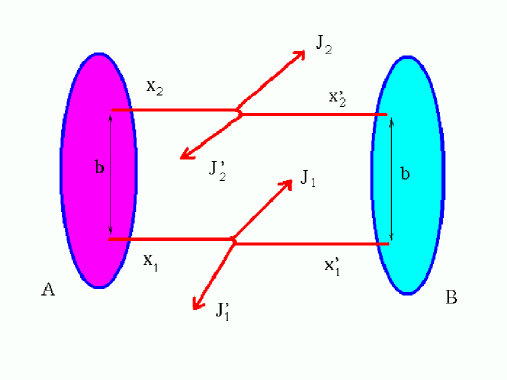
σ2=Γ1(x1,x2,b;M12,M22)σp(x1w1)σp(x2w2)Γ2(w1,w2,b;M12,M22)𝑑x1𝑑w1𝑑x2𝑑w2d2bsubscript𝜎2subscriptΓ1subscript𝑥1subscript𝑥2𝑏superscriptsubscript𝑀12superscriptsubscript𝑀22subscript𝜎𝑝subscript𝑥1subscript𝑤1subscript𝜎𝑝subscript𝑥2subscript𝑤2subscriptΓ2subscript𝑤1subscript𝑤2𝑏superscriptsubscript𝑀12superscriptsubscript𝑀22differential-dsubscript𝑥1differential-dsubscript𝑤1differential-dsubscript𝑥2differential-dsubscript𝑤2superscript𝑑2𝑏\sigma_{2}=\int\Gamma_{1}(x_{1},x_{2},b;M_{1}^{2},M_{2}^{2})\sigma_{p}(x_{1}w_{1})\sigma_{p}(x_{2}w_{2})\Gamma_{2}(w_{1},w_{2},b;M_{1}^{2},M_{2}^{2})dx_{1}dw_{1}dx_{2}dw_{2}d^{2}b (22)

with the geometrical interpretation shown in fig.4. Notice that the normalization contains also the multiplicity factor which counts the number of parton interactions in the hadronic collision (two in this case).

III Double parton distributions in the BFKL regime

A Emission of a jet from a single BFKL chain

In the framework of the hard pomeron model the hard collision process is associated to the production of a gluon with sufficiently large transverse momentum k>kmin𝑘subscript𝑘𝑚𝑖𝑛k>k_{min} and at a given rapidity (In this section only 2-dimensional transverse vectors will appear, so that we again omit the subindex perpendicular-to\perp and one take the metric Euclidean, k20superscript𝑘20k^{2}\geq 0).

The emission of a gluon with momentum k𝑘k is described by modifying as follows the BFKL Green function in coordinates space G(r,r′′)𝐺superscript𝑟superscript𝑟′′G(r^{\prime},r^{\prime\prime})[8]:

G(r,r′′)d2rG(rr)V(k)G(r,r′′)𝐺superscript𝑟superscript𝑟′′superscript𝑑2𝑟𝐺superscript𝑟𝑟𝑉𝑘𝐺𝑟superscript𝑟′′G(r^{\prime},r^{\prime\prime})\rightarrow\int d^{2}rG(r^{\prime}r)V(k)G(r,r^{\prime\prime}) (23)

where r𝑟r’s are relative distances between the gluons and

Vk(r)=12αsk2ΔeikrΔsubscript𝑉𝑘𝑟12subscript𝛼𝑠superscript𝑘2superscriptΔsuperscript𝑒𝑖𝑘𝑟superscriptΔabsentV_{k}(r)=\frac{12\alpha_{s}}{k^{2}}\stackrel{{\scriptstyle\leftarrow}}{{\Delta}}e^{ikr}\stackrel{{\scriptstyle\rightarrow}}{{\Delta}} (24)

is the vertex operator describing the emission of the gluon, the arrows show the direction of the action of the ΔΔ\Delta operators. The two BFKL Green functions in (23) are to be taken at appropriate energy (rapidity) ranges, corresponding to the rapidity distance of the emitted gluon from the projectile. This dependence is not written explicitly nor to overburden our formulas with arguments and/or indices.

The first step is to generalize Eq.(23) for the non-forward BFKL chain. In momentum space the emission of a gluon with momentum k𝑘k is described by the vertex

V(l1,l2|l1,l2)𝑉subscript𝑙1conditionalsubscript𝑙2subscriptsuperscript𝑙1subscriptsuperscript𝑙2\displaystyle V(l_{1},l_{2}|l^{\prime}_{1},l^{\prime}_{2}) (25)
=\displaystyle= 6αsk2(2π)2δ2(12(l1+l2l1l2)k)(l12l22+l22l12k2(l1l2)2)6subscript𝛼𝑠superscript𝑘2superscript2𝜋2superscript𝛿212subscript𝑙1subscript𝑙2subscriptsuperscript𝑙1subscriptsuperscript𝑙2𝑘superscriptsubscript𝑙12superscriptsubscriptsuperscript𝑙22superscriptsubscript𝑙22superscriptsubscriptsuperscript𝑙12superscript𝑘2superscriptsubscript𝑙1subscript𝑙22\displaystyle\frac{6\alpha_{s}}{k^{2}}(2\pi)^{2}\delta^{2}\left(\frac{1}{2}(l_{1}+l_{2}-l^{\prime}_{1}-l^{\prime}_{2})-k\right)\Big{(}l_{1}^{2}{l^{\prime}_{2}}^{2}+l_{2}^{2}{l^{\prime}_{1}}^{2}-{k^{2}}(l_{1}-l_{2})^{2}\Big{)} (26)

So the emission blob in momentum space Zk(q1,q2|q1,q2)subscript𝑍𝑘subscript𝑞1conditionalsubscript𝑞2subscriptsuperscript𝑞1subscriptsuperscript𝑞2Z_{k}(q_{1},q_{2}|q^{\prime}_{1},q^{\prime}_{2}) is given by

Zk(q1,q2|q1,q2)subscript𝑍𝑘subscript𝑞1conditionalsubscript𝑞2subscriptsuperscript𝑞1subscriptsuperscript𝑞2\displaystyle Z_{k}(q_{1},q_{2}|q^{\prime}_{1},q^{\prime}_{2}) =\displaystyle= 6αsk2i=12d2li(2π)2d2li(2π)2(2π)2δ2(12(l1+l2l1l2)k)6subscript𝛼𝑠superscript𝑘2superscriptsubscriptproduct𝑖12superscript𝑑2subscript𝑙𝑖superscript2𝜋2superscript𝑑2subscriptsuperscript𝑙𝑖superscript2𝜋2superscript2𝜋2superscript𝛿212subscript𝑙1subscript𝑙2subscriptsuperscript𝑙1subscriptsuperscript𝑙2𝑘\displaystyle\frac{6\alpha_{s}}{k^{2}}\int\prod_{i=1}^{2}\frac{d^{2}l_{i}}{(2\pi)^{2}}\frac{d^{2}l^{\prime}_{i}}{(2\pi)^{2}}(2\pi)^{2}\delta^{2}\left(\frac{1}{2}(l_{1}+l_{2}-l^{\prime}_{1}-l^{\prime}_{2})-k\right) (27)
×\displaystyle\times (l12l22+l22l12k2(l1l2)2)G(q1,q2|l1,l2)G(l1,l2|q1q2)superscriptsubscript𝑙12superscriptsubscriptsuperscript𝑙22superscriptsubscript𝑙22superscriptsubscriptsuperscript𝑙12superscript𝑘2superscriptsubscript𝑙1subscript𝑙22𝐺subscript𝑞1conditionalsubscript𝑞2subscript𝑙1subscript𝑙2𝐺subscriptsuperscript𝑙1conditionalsubscriptsuperscript𝑙2subscriptsuperscript𝑞1subscriptsuperscript𝑞2\displaystyle\Big{(}l_{1}^{2}{l^{\prime}_{2}}^{2}+l_{2}^{2}{l^{\prime}_{1}}^{2}-{k^{2}}(l_{1}-l_{2})^{2}\Big{)}G(q_{1},q_{2}|l_{1},l_{2})G(l^{\prime}_{1},l^{\prime}_{2}|q^{\prime}_{1}q^{\prime}_{2}) (28)
×\displaystyle\times (2π)2δ2(q1q2l1+l2)(2π)2δ2(l1l2q1+q2)superscript2𝜋2superscript𝛿2subscript𝑞1subscript𝑞2subscript𝑙1subscript𝑙2superscript2𝜋2superscript𝛿2subscriptsuperscript𝑙1subscriptsuperscript𝑙2subscriptsuperscript𝑞1subscriptsuperscript𝑞2\displaystyle(2\pi)^{2}\delta^{2}(q_{1}-q_{2}-l_{1}+l_{2})(2\pi)^{2}\delta^{2}(l^{\prime}_{1}-l^{\prime}_{2}-q^{\prime}_{1}+q^{\prime}_{2}) (29)

In coordinates space one writes:

(2π)2δ2(q1q2l1\displaystyle(2\pi)^{2}\delta^{2}(q_{1}-q_{2}-l_{1} +\displaystyle+ l2)G(q1,q2|l1,l2)\displaystyle l_{2})G(q_{1},q_{2}|l_{1},l_{2}) (30)
=\displaystyle= i=12d2rid2ziG(r1,r2|z1,z2)e(iq1r1+iq2r2+il1z1il2z2)superscriptsubscriptproduct𝑖12superscript𝑑2subscript𝑟𝑖superscript𝑑2subscript𝑧𝑖𝐺subscript𝑟1conditionalsubscript𝑟2subscript𝑧1subscript𝑧2superscript𝑒𝑖subscript𝑞1subscript𝑟1𝑖subscript𝑞2subscript𝑟2𝑖subscript𝑙1subscript𝑧1𝑖subscript𝑙2subscript𝑧2\displaystyle\int\prod_{i=1}^{2}d^{2}r_{i}d^{2}z_{i}G(r_{1},r_{2}|z_{1},z_{2})e^{(-iq_{1}r_{1}+iq_{2}r_{2}+il_{1}z_{1}-il_{2}z_{2})} (31)

and

(2π)2δ2(l1l2q1\displaystyle(2\pi)^{2}\delta^{2}(l^{\prime}_{1}-l^{\prime}_{2}-q^{\prime}_{1} +\displaystyle+ q2)G(l1,l2|q1,q2)\displaystyle q^{\prime}_{2})G(l^{\prime}_{1},l^{\prime}_{2}|q^{\prime}_{1},q^{\prime}_{2}) (32)
=\displaystyle= i=12d2rid2ziG(z1,z2|r1,r2)e(il1z1+il2z2+iq1r1iq2r2)superscriptsubscriptproduct𝑖12superscript𝑑2subscriptsuperscript𝑟𝑖superscript𝑑2subscriptsuperscript𝑧𝑖𝐺subscriptsuperscript𝑧1conditionalsubscriptsuperscript𝑧2subscriptsuperscript𝑟1subscriptsuperscript𝑟2superscript𝑒𝑖subscriptsuperscript𝑙1subscriptsuperscript𝑧1𝑖subscriptsuperscript𝑙2subscriptsuperscript𝑧2𝑖subscriptsuperscript𝑞1subscriptsuperscript𝑟1𝑖subscriptsuperscript𝑞2subscriptsuperscript𝑟2\displaystyle\int\prod_{i=1}^{2}d^{2}r^{\prime}_{i}d^{2}z^{\prime}_{i}G(z^{\prime}_{1},z^{\prime}_{2}|r^{\prime}_{1},r^{\prime}_{2})e^{(-il^{\prime}_{1}z^{\prime}_{1}+il^{\prime}_{2}z^{\prime}_{2}+iq^{\prime}_{1}r^{\prime}_{1}-iq^{\prime}_{2}r^{\prime}_{2})} (33)

Note that due to the inclusion of the δ𝛿\delta function in the Fourier transforms (25) and (26), the Green functions in coordinate space are translationally invariant:

G(r1+a,r2+a|z1+a,z2+a)=G(r1,r2|z1,z2)𝐺subscript𝑟1𝑎subscript𝑟2conditional𝑎subscript𝑧1𝑎subscript𝑧2𝑎𝐺subscript𝑟1conditionalsubscript𝑟2subscript𝑧1subscript𝑧2G(r_{1}+a,r_{2}+a|z_{1}+a,z_{2}+a)=G(r_{1},r_{2}|z_{1},z_{2}) (34)

The momenta squared in the emission vertex are substituted by differential operators applied to the Green function. The bracket in (24) is written as


Δ1Δ2+Δ2Δ1+k2(1+2)(1+2)subscriptΔ1subscriptsuperscriptΔ2subscriptΔ2subscriptsuperscriptΔ1superscript𝑘2subscript1subscript2subscriptsuperscript1subscriptsuperscript2\displaystyle\Delta_{1}\Delta^{\prime}_{2}+\Delta_{2}\Delta^{\prime}_{1}+k^{2}(\nabla_{1}+\nabla_{2})(\nabla^{\prime}_{1}+\nabla^{\prime}_{2})

where one uses the notation Δ1=Δ(z1)subscriptΔ1Δsubscript𝑧1\Delta_{1}=\Delta(z_{1}), Δ1=Δ(z1)subscriptsuperscriptΔ1Δsubscriptsuperscript𝑧1\Delta^{\prime}_{1}=\Delta(z^{\prime}_{1}) etc. The remaining δ𝛿\delta function in Eq.(24) is represented as an integral


(2π)2δ2((l1+l2l1l2)/2k)=d2zeiz((l1+l2l1l2)/2k)superscript2𝜋2superscript𝛿2subscript𝑙1subscript𝑙2subscriptsuperscript𝑙1subscriptsuperscript𝑙22𝑘superscript𝑑2𝑧superscript𝑒𝑖𝑧subscript𝑙1subscript𝑙2subscriptsuperscript𝑙1subscriptsuperscript𝑙22𝑘\displaystyle(2\pi)^{2}\delta^{2}((l_{1}+l_{2}-l^{\prime}_{1}-l^{\prime}_{2})/2-k)=\int d^{2}ze^{-iz((l_{1}+l_{2}-l^{\prime}_{1}-l^{\prime}_{2})/2-k)}

in such a way that the integrations over the four transverse momenta in Eq.(24) produce four δ𝛿\delta functions in coordinate space:


δ2(z1z/2),δ2(z2+z/2),δ2(z1z/2),δ2(z2+z/2)superscript𝛿2subscript𝑧1𝑧2superscript𝛿2subscript𝑧2𝑧2superscript𝛿2subscriptsuperscript𝑧1𝑧2superscript𝛿2subscriptsuperscript𝑧2𝑧2\displaystyle\delta^{2}(z_{1}-z/2),\ \ \delta^{2}(z_{2}+z/2),\ \ \delta^{2}(z^{\prime}_{1}-z/2),\ \ \delta^{2}(z^{\prime}_{2}+z/2)

One obtains therefore


Zk(q1,q2|q1,q2)=i=12d2rid2rie(iq1r1+iq2r2+iq1r1iq2r2)d2z[G(r1,r2|z1,z2)6αsk2eikz\displaystyle Z_{k}(q_{1},q_{2}|q^{\prime}_{1},q^{\prime}_{2})=\int\prod_{i=1}^{2}d^{2}r_{i}d^{2}r^{\prime}_{i}e^{(-iq_{1}r_{1}+iq_{2}r_{2}+iq^{\prime}_{1}r^{\prime}_{1}-iq^{\prime}_{2}r^{\prime}_{2})}d^{2}z\Big{[}G(r_{1},r_{2}|z_{1},z_{2})\frac{6\alpha_{s}}{k^{2}}e^{ikz}

×(Δ1Δ2+Δ2Δ1+k2(1+2)(1+2))G(z1,z2|r1,r2)]z1=z1=z2,z2=z2=z2\times(\Delta_{1}\Delta^{\prime}_{2}+\Delta_{2}\Delta^{\prime}_{1}+k^{2}(\nabla_{1}+\nabla_{2})(\nabla^{\prime}_{1}+\nabla^{\prime}_{2}))G(z^{\prime}_{1},z^{\prime}_{2}|r^{\prime}_{1},r^{\prime}_{2})\Big{]}_{z_{1}=z^{\prime}_{1}=\frac{z}{2},z_{2}=z^{\prime}_{2}=-\frac{z}{2}} (35)

and the differential operator which stands between the two Green functions is precisely the generalization of the emission operator Vksubscript𝑉𝑘V_{k} to the non-forward case. By using the notation:


G(r1,r2|z2,z2)Vk(z)G(z2,z2|r1,r2)[G(r1,r2|z1,z2)6αsk2eikz\displaystyle G\Big{(}r_{1},r_{2}\Big{|}\frac{z}{2},-\frac{z}{2}\Big{)}V_{k}(z)G\Big{(}\frac{z}{2},-\frac{z}{2}\Big{|}r^{\prime}_{1},r^{\prime}_{2}\Big{)}\equiv\Big{[}G(r_{1},r_{2}|z_{1},z_{2})\frac{6\alpha_{s}}{k^{2}}e^{ikz}

×(Δ1Δ2+Δ2Δ1+k2(1+2)(1+2))G(z1,z2|r1,r2)]z1=z1=z2,z2=z2=z2\times(\Delta_{1}\Delta^{\prime}_{2}+\Delta_{2}\Delta^{\prime}_{1}+k^{2}(\nabla_{1}+\nabla_{2})(\nabla^{\prime}_{1}+\nabla^{\prime}_{2}))G(z^{\prime}_{1},z^{\prime}_{2}|r^{\prime}_{1},r^{\prime}_{2})\Big{]}_{z_{1}=z^{\prime}_{1}=\frac{z}{2},z_{2}=z^{\prime}_{2}=-\frac{z}{2}} (36)

one may rewrite Eq.(28) in a more compact form

Zk(q1,q2|q1,q2)=i=12subscript𝑍𝑘subscript𝑞1conditionalsubscript𝑞2subscriptsuperscript𝑞1subscriptsuperscript𝑞2superscriptsubscriptproduct𝑖12\displaystyle Z_{k}(q_{1},q_{2}|q^{\prime}_{1},q^{\prime}_{2})=\int\prod_{i=1}^{2} d2rid2rie(iq1r1+iq2r2+iq1r1iq2r2)d2zsuperscript𝑑2subscript𝑟𝑖superscript𝑑2subscriptsuperscript𝑟𝑖superscript𝑒𝑖subscript𝑞1subscript𝑟1𝑖subscript𝑞2subscript𝑟2𝑖subscriptsuperscript𝑞1subscriptsuperscript𝑟1𝑖subscriptsuperscript𝑞2subscriptsuperscript𝑟2superscript𝑑2𝑧\displaystyle d^{2}r_{i}d^{2}r^{\prime}_{i}e^{(-iq_{1}r_{1}+iq_{2}r_{2}+iq^{\prime}_{1}r^{\prime}_{1}-iq^{\prime}_{2}r^{\prime}_{2})}d^{2}z (38)
×G(r1,r2|z2,z2)Vk(z)G(z2,z2|r1,r2)absent𝐺subscript𝑟1conditionalsubscript𝑟2𝑧2𝑧2subscript𝑉𝑘𝑧𝐺𝑧2conditional𝑧2subscriptsuperscript𝑟1subscriptsuperscript𝑟2\displaystyle\times G\Big{(}r_{1},r_{2}\Big{|}\frac{z}{2},-\frac{z}{2}\Big{)}V_{k}(z)G\Big{(}\frac{z}{2},-\frac{z}{2}\Big{|}r^{\prime}_{1},r^{\prime}_{2}\Big{)}

One defines Z𝑍Z in coordinates space in the following way:

Zk(r1,r2|r1,r2)subscript𝑍𝑘subscript𝑟1conditionalsubscript𝑟2subscriptsuperscript𝑟1subscriptsuperscript𝑟2\displaystyle Z_{k}(r_{1},r_{2}|r^{\prime}_{1},r^{\prime}_{2}) =\displaystyle= j=12d2qi(2π)2d2qj(2π)2superscriptsubscriptproduct𝑗12superscript𝑑2subscript𝑞𝑖superscript2𝜋2superscript𝑑2subscriptsuperscript𝑞𝑗superscript2𝜋2\displaystyle\int\prod_{j=1}^{2}\frac{d^{2}q_{i}}{(2\pi)^{2}}\frac{d^{2}q^{\prime}_{j}}{(2\pi)^{2}} (39)
×\displaystyle\times (2π)2δ(q1q2q1+q2)Zk(q1,q2|q1,q2)e(iq1r1iq2r2iq1r1+iq2r2)superscript2𝜋2𝛿subscript𝑞1subscript𝑞2subscriptsuperscript𝑞1subscriptsuperscript𝑞2subscript𝑍𝑘subscript𝑞1conditionalsubscript𝑞2subscriptsuperscript𝑞1subscriptsuperscript𝑞2superscript𝑒𝑖subscript𝑞1subscript𝑟1𝑖subscript𝑞2subscript𝑟2𝑖subscriptsuperscript𝑞1subscriptsuperscript𝑟1𝑖subscriptsuperscript𝑞2subscriptsuperscript𝑟2\displaystyle(2\pi)^{2}\delta(q_{1}-q_{2}-q^{\prime}_{1}+q^{\prime}_{2})Z_{k}(q_{1},q_{2}|q^{\prime}_{1},q^{\prime}_{2})e^{(iq_{1}r_{1}-iq_{2}r_{2}-iq^{\prime}_{1}r^{\prime}_{1}+iq^{\prime}_{2}r^{\prime}_{2})} (40)

By expressing the δ𝛿\delta function as an integral over the impact parameters B𝐵B

(2π)2δ(q1q2q1+q2)=d2BeiB(q1q2q1+q2)superscript2𝜋2𝛿subscript𝑞1subscript𝑞2subscriptsuperscript𝑞1subscriptsuperscript𝑞2superscript𝑑2𝐵superscript𝑒𝑖𝐵subscript𝑞1subscript𝑞2subscriptsuperscript𝑞1subscriptsuperscript𝑞2(2\pi)^{2}\delta(q_{1}-q_{2}-q^{\prime}_{1}+q^{\prime}_{2})=\int d^{2}Be^{-iB(q_{1}-q_{2}-q^{\prime}_{1}+q^{\prime}_{2})} (41)

and by using (32) and (34) in (33) one can do all integrations with the exception of those on B𝐵B and z𝑧z. The result is

Zk(r1,r2|r1,r2)subscript𝑍𝑘subscript𝑟1conditionalsubscript𝑟2subscriptsuperscript𝑟1subscriptsuperscript𝑟2\displaystyle Z_{k}(r_{1},r_{2}|r^{\prime}_{1},r^{\prime}_{2}) (42)
=d2Bd2absentsuperscript𝑑2𝐵superscript𝑑2\displaystyle=\int d^{2}Bd^{2} z𝑧\displaystyle z G(r1+B,r2+B|z2,z2)Vk(z)G(z2,z2|r1+B,r2+B)𝐺subscript𝑟1𝐵subscript𝑟2conditional𝐵𝑧2𝑧2subscript𝑉𝑘𝑧𝐺𝑧2conditional𝑧2subscriptsuperscript𝑟1𝐵subscriptsuperscript𝑟2𝐵\displaystyle G\Bigl{(}r_{1}+B,r_{2}+B\Big{|}\frac{z}{2},-\frac{z}{2}\Bigr{)}V_{k}(z)G\Bigl{(}\frac{z}{2},-\frac{z}{2}\Big{|}r^{\prime}_{1}+B,r^{\prime}_{2}+B\Bigr{)} (43)

and, as a function of the c.m and relative coordinates,

Zk(R,r|R,r)=d2Bd2zG(R+B,r|0,z)Vk(z)G(0,z|R+B,r)subscript𝑍𝑘𝑅conditional𝑟superscript𝑅superscript𝑟superscript𝑑2𝐵superscript𝑑2𝑧𝐺𝑅𝐵conditional𝑟0𝑧subscript𝑉𝑘𝑧𝐺0conditional𝑧superscript𝑅𝐵superscript𝑟Z_{k}(R,r|R^{\prime},r^{\prime})=\int d^{2}Bd^{2}zG(R+B,r|0,z)V_{k}(z)G(0,z|R^{\prime}+B,r^{\prime}) (44)

showing that Zksubscript𝑍𝑘Z_{k} is translationally invariant:

Zk(R,r|R,r)=Zk(R+B,r|R+B,r)=Zk(RR,r,r)subscript𝑍𝑘𝑅conditional𝑟superscript𝑅superscript𝑟subscript𝑍𝑘𝑅𝐵conditional𝑟superscript𝑅𝐵superscript𝑟subscript𝑍𝑘𝑅superscript𝑅𝑟superscript𝑟Z_{k}(R,r|R^{\prime},r^{\prime})=Z_{k}(R+B,r|R^{\prime}+B,r^{\prime})=Z_{k}(R-R^{\prime},r,r^{\prime}) (45)

Eq. (37) is our final expression. It shows how one should change a BFKL Green function G(R,r|R,r)=G(RR,r,r)𝐺𝑅conditional𝑟superscript𝑅superscript𝑟𝐺𝑅superscript𝑅𝑟superscript𝑟G(R,r|R^{\prime},r^{\prime})=G(R-R^{\prime},r,r^{\prime}) to describe the emission of a gluon from the BFKL chain.

B Single parton distributions

The simplest case to consider in the BFKL formalism is the inclusive emission of a gluon. The problem has been extensively studied in the literature[9]. Here we approach the problem from a somewhat novel point of view, introducing the single parton densities in coordinates space in the BFKL framework. The quantities which are factorized in the BFKL formalism are the ‘unintegrated gluon densities’[10], depending explicitly on the transverse momentum of the interacting gluon. The distributions that will be discussed hereafter are therefore different as compared to the distributions discussed in the first part of the paper, since they depend explicitly on the distance in transverse space between the initial and the final interacting partons. The latter distributions are therefore obtained only after integration on this transverse distance, with 1/k1𝑘1/k as a lower limit.

Rather than using the known expression for the inclusive cross-section in terms of forward BFKL Green functions, one starts form the amplitude, corresponding to the exchange of any number of pomerons between the projectile and target, obtained in the approximation of a large number of colors N𝑁N and assuming the coupling of pomerons to the colliding particles as purely perturbative[11]. The amplitude is written as

𝒜=2isd2Rd2rd2rρp(r)ρq(r)(1e12g4Gs(R,r,r))𝒜2𝑖𝑠superscript𝑑2𝑅superscript𝑑2𝑟superscript𝑑2superscript𝑟subscript𝜌𝑝𝑟subscript𝜌𝑞superscript𝑟1superscript𝑒12superscript𝑔4subscript𝐺𝑠𝑅𝑟superscript𝑟{\cal A}=2is\int\,d^{2}R\int d^{2}r\int d^{2}r^{\prime}\rho_{p}(r)\rho_{q}(r^{\prime})\Big{(}1-e^{-\frac{1}{2}g^{4}G_{s}(R,r,r^{\prime})}\Big{)} (46)

Here ρp(q)(r)subscript𝜌𝑝𝑞𝑟\rho_{p(q)}(r) are the color densities of the projectile and of the target (with momenta p𝑝p and q𝑞q respectively). The function Gs(R,r,r)=G(R,r|0,r)subscript𝐺𝑠𝑅𝑟superscript𝑟𝐺𝑅conditional𝑟0superscript𝑟G_{s}(R,r,r^{\prime})=G(R,r|0,r^{\prime}) is the BFKL Green function, depending on the Mandelstam invariant s𝑠s. When retaining the s𝑠s-wave only, because of the azimuthal symmetry, it takes the form[12]

Gs(R,r,r)=1(2π)4𝑑νν2sE(ν)(ν2+1/4)2d2r0(rr10r20)1+2iν(rr10r20)12iνsubscript𝐺𝑠𝑅𝑟superscript𝑟1superscript2𝜋4differential-d𝜈superscript𝜈2superscript𝑠𝐸𝜈superscriptsuperscript𝜈2142superscript𝑑2subscript𝑟0superscript𝑟subscript𝑟10subscript𝑟2012𝑖𝜈superscriptsuperscript𝑟subscriptsuperscript𝑟10subscriptsuperscript𝑟2012𝑖𝜈G_{s}(R,r,r^{\prime})=\frac{1}{(2\pi)^{4}}\int d\nu\frac{\nu^{2}s^{-E(\nu)}}{(\nu^{2}+1/4)^{2}}\int d^{2}r_{0}\left(\frac{r}{r_{10}r_{20}}\right)^{1+2i\nu}\left(\frac{r^{\prime}}{r^{\prime}_{10}r^{\prime}_{20}}\right)^{1-2i\nu} (47)

where


r10=R+r/2r0,r20=Rr/2r0,r10=r/2r0,r20=r/2r0formulae-sequencesubscript𝑟10𝑅𝑟2subscript𝑟0formulae-sequencesubscript𝑟20𝑅𝑟2subscript𝑟0formulae-sequencesubscriptsuperscript𝑟10superscript𝑟2subscript𝑟0subscriptsuperscript𝑟20superscript𝑟2subscript𝑟0\displaystyle r_{10}=R+r/2-r_{0},\ r_{20}=R-r/2-r_{0},\ r^{\prime}_{10}=r^{\prime}/2-r_{0},\ r^{\prime}_{20}=-r^{\prime}/2-r_{0}

and E(ν)𝐸𝜈E(\nu) is the BFKL pomeron energy

E(ν)=(3g2/2π2)(Reψ(1/2+iν)ψ(1))𝐸𝜈3superscript𝑔22superscript𝜋2Re𝜓12𝑖𝜈𝜓1E(\nu)=(3g^{2}/2\pi^{2})({\rm Re}\,\psi(1/2+i\nu)-\psi(1)) (48)

Eq.(38) allows us to write down easily the amplitudes for single, double etc. pomeron exchange processes. The single BFKL pomeron exchange amplitude is written as

𝒜1=isg4αs2d2Rd2rd2rρp(r)ρq(r)Gs(R,r,r)subscript𝒜1𝑖𝑠superscript𝑔4superscriptsubscript𝛼𝑠2superscript𝑑2𝑅superscript𝑑2𝑟superscript𝑑2superscript𝑟subscript𝜌𝑝𝑟subscript𝜌𝑞superscript𝑟subscript𝐺𝑠𝑅𝑟superscript𝑟{\cal A}_{1}=isg^{4}\alpha_{s}^{2}\int\,d^{2}R\int d^{2}r\int d^{2}r^{\prime}\rho_{p}(r)\rho_{q}(r^{\prime})G_{s}(R,r,r^{\prime}) (49)

where the factor g4superscript𝑔4g^{4} corresponds to the couplings of the pomeron to the color densities ρ𝜌\rho. The inclusive cross-section for emission of a single gluon has therefore the form


I(k)=(2π)2d3σdyd2k=g4d2Rd2rd2rρp(r)ρq(r)Zk(R,r,r)𝐼𝑘superscript2𝜋2superscript𝑑3𝜎𝑑𝑦superscript𝑑2𝑘superscript𝑔4superscript𝑑2𝑅superscript𝑑2𝑟superscript𝑑2superscript𝑟subscript𝜌𝑝𝑟subscript𝜌𝑞superscript𝑟subscript𝑍𝑘𝑅𝑟superscript𝑟\displaystyle I(k)=\frac{(2\pi)^{2}d^{3}\sigma}{dyd^{2}k}=g^{4}\int\,d^{2}R\int d^{2}r\int d^{2}r^{\prime}\rho_{p}(r)\rho_{q}(r^{\prime})Z_{k}(R,r,r^{\prime})


=d2Rd2rd2rg2ρp(r)g2ρq(r)d2Bd2zGs1(R+B,r|0,z)Vk(z)Gs2(0,z|B,r)absentsuperscript𝑑2𝑅superscript𝑑2𝑟superscript𝑑2superscript𝑟superscript𝑔2subscript𝜌𝑝𝑟superscript𝑔2subscript𝜌𝑞superscript𝑟superscript𝑑2𝐵superscript𝑑2𝑧subscript𝐺subscript𝑠1𝑅𝐵conditional𝑟0𝑧subscript𝑉𝑘𝑧subscript𝐺subscript𝑠20conditional𝑧𝐵superscript𝑟\displaystyle=\int\,d^{2}R\int d^{2}r\int d^{2}r^{\prime}g^{2}\rho_{p}(r)g^{2}\rho_{q}(r^{\prime})d^{2}Bd^{2}zG_{s_{1}}(R+B,r|0,z)V_{k}(z)G_{s_{2}}(0,z|B,r^{\prime})

=d2Rd2Rd2zd2rd2rg2ρp(r)g2ρq(r)Gs1(R,r|0,z)Vk(z)Gs2(0,z|R,r)absentsuperscript𝑑2𝑅superscript𝑑2superscript𝑅superscript𝑑2𝑧superscript𝑑2𝑟superscript𝑑2superscript𝑟superscript𝑔2subscript𝜌𝑝𝑟superscript𝑔2subscript𝜌𝑞superscript𝑟subscript𝐺subscript𝑠1𝑅conditional𝑟0𝑧subscript𝑉𝑘𝑧subscript𝐺subscript𝑠20conditional𝑧superscript𝑅superscript𝑟=\int\,d^{2}Rd^{2}R^{\prime}d^{2}z\int d^{2}r\int d^{2}r^{\prime}g^{2}\rho_{p}(r)g^{2}\rho_{q}(r^{\prime})G_{s_{1}}(R,r|0,z)V_{k}(z)G_{s_{2}}(0,z|R^{\prime},r^{\prime}) (50)

The dependence on energy is written explicitly in the Green functions. The emitted gluon rapidity (relative to the target) is y=logs2𝑦subscript𝑠2y=\log s_{2}. Then s1=s/s2subscript𝑠1𝑠subscript𝑠2s_{1}=s/s_{2} (the scale is not defined in the theory, as usual one takes it as 1 GeV). The integrated single hard scattering inclusive cross section can be written as


σ1=𝑑yd2kI(k)=d2k01𝑑x𝑑wδ(xwk2s)I(k)subscript𝜎1differential-d𝑦superscript𝑑2𝑘𝐼𝑘superscript𝑑2𝑘superscriptsubscript01differential-d𝑥differential-d𝑤𝛿𝑥𝑤superscript𝑘2𝑠𝐼𝑘\displaystyle\sigma_{1}=\int dyd^{2}kI(k)=\int d^{2}k\int_{0}^{1}dxdw\delta\left(xw-\frac{k^{2}}{s}\right)I(k)

where one has introduced the scaling variables x=s1/s𝑥subscript𝑠1𝑠x=s_{1}/s and w=s2/s𝑤subscript𝑠2𝑠w=s_{2}/s. By comparing the expression above with the factorization formula one obtains the expression for the partonic density of the projectile

Fp(x,R,z)=g2d2rρp(r)Gs1(R,r,z)subscript𝐹𝑝𝑥𝑅𝑧superscript𝑔2superscript𝑑2𝑟subscript𝜌𝑝𝑟subscript𝐺subscript𝑠1𝑅𝑟𝑧F_{p}(x,R,z)=g^{2}\int d^{2}r\rho_{p}(r)G_{s_{1}}(R,r,z) (51)

with x=s/s1𝑥𝑠subscript𝑠1x=s/s_{1} and G(R,r,z)=G(R,r|0,z)𝐺𝑅𝑟𝑧𝐺𝑅conditional𝑟0𝑧G(R,r,z)=G(R,r|0,z).

The meaning of the variables is the following: R𝑅R is the distance from the center of the projectile and z𝑧z the distance between the initial and the final interacting partons. The size of z𝑧z is of order of 1/k1𝑘1/k, as a result of the factor expikz𝑖𝑘𝑧\exp ikz in the hard interaction vertex, and the size of r𝑟r is of the order of the dimensions of the projectile. The perturbative approach is justified when both r𝑟r and z𝑧z are small. The asymptotics of the Green function G𝐺G for small relative distances and large energy was obtained in[11]. The resulting expression is a function of the dimensionless variable ξ=R2/rr(>>1\xi=R^{2}/rr^{\prime}(>>1):

Gs(R,r,r)r,r<<RsΔπ5/2(alns)3/2ξ1lnξexp(ln2ξalns)similar-to-or-equalssubscript𝐺𝑠subscript𝑅𝑟superscript𝑟much-less-than𝑟superscript𝑟𝑅superscript𝑠Δsuperscript𝜋52superscript𝑎𝑠32superscript𝜉1𝜉superscript2𝜉𝑎𝑠G_{s}(R,r,r^{\prime})_{r,r^{\prime}<<R}\simeq\frac{s^{\Delta}}{\pi^{5/2}(a\ln s)^{3/2}}\xi^{-1}\ln\xi\exp\left(-\frac{\ln^{2}\xi}{a\ln s}\right) (52)

where ΔΔ\Delta is the BFKL intercept

Δ=12αsπln2Δ12subscript𝛼𝑠𝜋2\Delta=\frac{12\alpha_{s}}{\pi}\ln 2 (53)

and

a=42αsπζ(3)𝑎42subscript𝛼𝑠𝜋𝜁3a=\frac{42\alpha_{s}}{\pi}\zeta(3) (54)

With z𝑧z small and fixed, the partonic density (43) behaves as

Fp(x,R,z)(1/x)Δlog3/2(1/x)1R2logRexp(log2Ralog(1/x))similar-tosubscript𝐹𝑝𝑥𝑅𝑧superscript1𝑥Δsuperscript321𝑥1superscript𝑅2𝑅superscript2𝑅𝑎1𝑥F_{p}(x,R,z)\sim\frac{(1/x)^{\Delta}}{\log^{3/2}(1/x)}\frac{1}{R^{2}}\log R\exp\left(-\frac{\log^{2}R}{a\log(1/x)}\right) (55)

and it falls rather slowly (essentially as 1/R21superscript𝑅21/R^{2}) as a function of the distance from the center of the projectile (R𝑅R represents the distance from the projectile, whose average dimension r0=rsubscript𝑟0delimited-⟨⟩𝑟r_{0}=\langle r\rangle is much smaller than R𝑅R). The effect of the exponential is felt only at relatively large Rexp1/xsimilar-to𝑅1𝑥R\sim\exp\sqrt{1/x}. A more quantitative estimate of the density can be made by neglecting the weak dependence on r𝑟r in the logarithmic factors in (44) and by making the substitution rr0𝑟subscript𝑟0r\rightarrow r_{0}:

Fp(x,R,z)g2π5/2(1/x)Δ(aln(1/x))3/2zr0R2lnR2zr0exp(ln2(R2/zr0)aln(1/x))similar-to-or-equalssubscript𝐹𝑝𝑥𝑅𝑧superscript𝑔2superscript𝜋52superscript1𝑥Δsuperscript𝑎1𝑥32𝑧subscript𝑟0superscript𝑅2superscript𝑅2𝑧subscript𝑟0superscript2superscript𝑅2𝑧subscript𝑟0𝑎1𝑥F_{p}(x,R,z)\simeq\frac{g^{2}}{\pi^{5/2}}\frac{(1/x)^{\Delta}}{(a\ln(1/x))^{3/2}}\frac{zr_{0}}{R^{2}}\ln\frac{R^{2}}{zr_{0}}\exp\left(-\frac{\ln^{2}(R^{2}/zr_{0})}{a\ln(1/x)}\right) (56)

An analogous expression can be written for the target.

C Two pomerons coupling to a qq¯𝑞¯𝑞q\bar{q} pair and triple pomeron

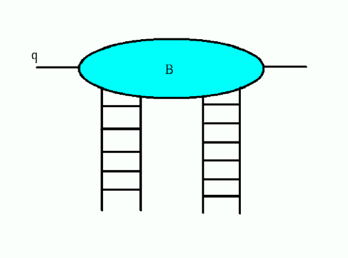
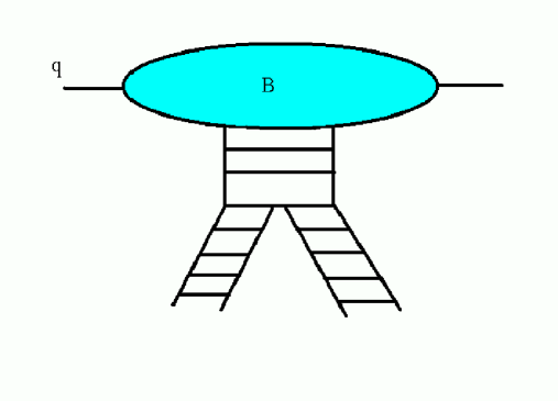
The general structure of the amplitude describing the double partonic density in the BFKL regime is shown in Fig.5, where one assigns the partons undergoing the two hard collisions to two different BFKL pomeron ladders. The coupling of the two pomerons to the projectile is described by the upper blob B𝐵B. One calls the energetic variable of the pomeron s2=s/s1subscript𝑠2𝑠subscript𝑠1s_{2}=s/s_{1}, with s𝑠s the overall c.m. energy squared, for simplicity one takes it to be the same for both legs. The upper blob B𝐵B is then integrated on s1subscript𝑠1s_{1}.

The asymptotic behavior of B(s1)𝐵subscript𝑠1B(s_{1}) is described by a single pomeron exchange, so that

B(s1)B(y1)=b(y1)eΔy1,y1=logs1formulae-sequence𝐵subscript𝑠1𝐵subscript𝑦1𝑏subscript𝑦1superscript𝑒Δsubscript𝑦1subscript𝑦1subscript𝑠1B(s_{1})\equiv B(y_{1})=b(y_{1})e^{\Delta y_{1}},\ \ y_{1}=\log s_{1} (57)

where ΔΔ\Delta is the pomeron intercept and b(y)𝑏𝑦b(y) is some smooth function tending to a constant at high y1subscript𝑦1y_{1}. Each of the pomeron legs has a similar behavior as a function of its energy variable s2subscript𝑠2s_{2}:

P(s2)P(y2)=p(y2)eΔy2,y2=logs2formulae-sequence𝑃subscript𝑠2𝑃subscript𝑦2𝑝subscript𝑦2superscript𝑒Δsubscript𝑦2subscript𝑦2subscript𝑠2P(s_{2})\equiv P(y_{2})=p(y_{2})e^{\Delta y_{2}},\ \ y_{2}=\log s_{2} (58)

with p(y2)𝑝subscript𝑦2p(y_{2}) a smooth function tending to a constant at high y2subscript𝑦2y_{2}. The amplitude of Fig.5 is given by a integral over y1subscript𝑦1y_{1}:

0Y𝑑y1B(y1)P1(Yy1)P2(Yy1)=e2ΔY0Y𝑑y1eΔy1b(y1)p1(Yy1)p2(Yy1)superscriptsubscript0𝑌differential-dsubscript𝑦1𝐵subscript𝑦1subscript𝑃1𝑌subscript𝑦1subscript𝑃2𝑌subscript𝑦1superscript𝑒2Δ𝑌superscriptsubscript0𝑌differential-dsubscript𝑦1superscript𝑒Δsubscript𝑦1𝑏subscript𝑦1subscript𝑝1𝑌subscript𝑦1subscript𝑝2𝑌subscript𝑦1\int_{0}^{Y}dy_{1}B(y_{1})P_{1}(Y-y_{1})P_{2}(Y-y_{1})=e^{2\Delta Y}\int_{0}^{Y}dy_{1}e^{-\Delta y_{1}}b(y_{1})p_{1}(Y-y_{1})p_{2}(Y-y_{1}) (59)

where Y=y1+y2=logs𝑌subscript𝑦1subscript𝑦2𝑠Y=y_{1}+y_{2}=\log s is the overall rapidity interval. As one may see, at very large Y𝑌Y values, the integration in (51) stays limited to the region where y1subscript𝑦1y_{1} is smaller or of the order 1/Δ1Δ1/\Delta and thus it is independent on Y𝑌Y. One may therefore take for p1(2)subscript𝑝12p_{1(2)} the asymptotic values and rewrite (51) as

e2ΔYp1asp2as0eΔy1b(y1)𝑑y1superscript𝑒2Δ𝑌superscriptsubscript𝑝1𝑎𝑠superscriptsubscript𝑝2𝑎𝑠superscriptsubscript0superscript𝑒Δsubscript𝑦1𝑏subscript𝑦1differential-dsubscript𝑦1e^{2\Delta Y}p_{1}^{as}p_{2}^{as}\int_{0}^{\infty}e^{-\Delta y_{1}}b(y_{1})dy_{1} (60)

which corresponds precisely to the behavior of a two pomeron exchange process.

The rapidities that dominate the integral (52) are of order 1/Δ1Δ1/\Delta. The actual value ΔΔ\Delta is however not well defined, since it is given by the coupling, whose value is a parameter in the BFKL approach. Rather than trying to determine which are the rapidities relevant to B𝐵B, we proceed by discussing two limiting cases.

If Q2superscript𝑄2Q^{2} is the virtuality of the interacting qq¯𝑞¯𝑞q{\bar{q}} pairs (which has to be large to justify the perturbative approach) a limiting configuration is reached when Q2superscript𝑄2Q^{2} is of the same order (or larger) than s1subscript𝑠1s_{1}, namely,

logQ2(or>)1/Δ<<Y\log Q^{2}\sim({\rm or}\,>)1/\Delta<<Y (61)

The blob B𝐵B enters then in the DGLAP regime (finite scaling variable x1subscript𝑥1x_{1}) where only the large logarithms log(Q2/Λ)superscript𝑄2Λ\log(Q^{2}/\Lambda) are to be considered. In the fixed coupling approach of BFKL these logarithms are neglected altogether. Within the present scale invariant model one does not need therefore to sum any logarithms and one may state within the pure perturbative approach. The upper blob is then simply reduced to the qq¯𝑞¯𝑞q\bar{q} pair, to which the pomerons are coupled directly. This is precisely the approximation which leads to the amplitude (36) obtained in[11] and which was used in the previous subsection.

On the other hand, at lower virtualities, such as

1<<logQ2<<1/Δmuch-less-than1superscript𝑄2much-less-than1Δ1<<\log Q^{2}<<1/\Delta (62)

the structure of the blob B𝐵B becomes important. Another limiting configuration is reached when B𝐵B enters in the BFKL regime, namely it is itself described by a pomeron, which has to eventually split into the two lower pomerons and the whole amplitude is described by a triple pomeron interaction. One should keep in mind that, in this last case, the three pomerons are not however in an equivalent regime. The two lower ones, as mentioned, may be taken at their asymptotical regime, Δy2>>1much-greater-thanΔsubscript𝑦21\Delta y_{2}>>1. The upper one, on the contrary, is characterized by much smaller energies, such that Δy11similar-toΔsubscript𝑦11\Delta y_{1}\sim 1, so that its exact form needs to be used.

The two limiting possibilities which we consider are therefore the direct coupling of the pomerons to the constituent quarks and the triple pomeron interaction. We first discuss the simpler direct coupling case.

D Two pomerons coupled directly to the projectile(target)

From the general expression of the amplitude (36) the contribution with two pomerons directly coupled both to the projectile and target is written as:

𝒜2=isg82d2Rd2rd2rρp(r)ρq(r)Gs2(R,r,r)subscript𝒜2𝑖𝑠superscript𝑔82superscript𝑑2𝑅superscript𝑑2𝑟superscript𝑑2superscript𝑟subscript𝜌𝑝𝑟subscript𝜌𝑞superscript𝑟superscriptsubscript𝐺𝑠2𝑅𝑟superscript𝑟{\cal A}_{2}=-is\frac{g^{8}}{2}\int\,d^{2}R\int d^{2}r\int d^{2}r^{\prime}\rho_{p}(r)\rho_{q}(r^{\prime})G_{s}^{2}(R,r,r^{\prime}) (63)

The integrated inclusive cross section is obtained by dividing the amplitude by s𝑠s and by taking the imaginary part with a minus sign:

σ2=g8d2Rd2rd2rρp(r)ρq(r)Gs2(R,r,r)subscript𝜎2superscript𝑔8superscript𝑑2𝑅superscript𝑑2𝑟superscript𝑑2superscript𝑟subscript𝜌𝑝𝑟subscript𝜌𝑞superscript𝑟superscriptsubscript𝐺𝑠2𝑅𝑟superscript𝑟\sigma_{2}=g^{8}\int\,d^{2}R\int d^{2}r\int d^{2}r^{\prime}\rho_{p}(r)\rho_{q}(r^{\prime})G_{s}^{2}(R,r,r^{\prime}) (64)

To obtain the double differential inclusive cross-section, corresponding to the emission of two hard gluons with momenta k1subscript𝑘1k_{1} and k2subscript𝑘2k_{2} from the two pomerons, we have to substitute the pomeronic Green function with the emission functions Zk1subscript𝑍subscript𝑘1Z_{k_{1}} and Zk2subscript𝑍subscript𝑘2Z_{k_{2}}. One obtains therefore


I(k1,k2)=(2π)2d3dy1d2k1(2π)2d3dy2d2k2σ𝐼subscript𝑘1subscript𝑘2superscript2𝜋2superscript𝑑3𝑑subscript𝑦1superscript𝑑2subscript𝑘1superscript2𝜋2superscript𝑑3𝑑subscript𝑦2superscript𝑑2subscript𝑘2𝜎\displaystyle I(k_{1},k_{2})=\frac{(2\pi)^{2}d^{3}}{dy_{1}d^{2}k_{1}}\frac{(2\pi)^{2}d^{3}}{dy_{2}d^{2}k_{2}}\sigma

g8d2Rd2rd2rρp(r)ρq(r)Zk1(R,r,r)Zk2(R,r,r)superscript𝑔8superscript𝑑2𝑅superscript𝑑2𝑟superscript𝑑2superscript𝑟subscript𝜌𝑝𝑟subscript𝜌𝑞superscript𝑟subscript𝑍subscript𝑘1𝑅𝑟superscript𝑟subscript𝑍subscript𝑘2𝑅𝑟superscript𝑟g^{8}\int d^{2}R\int d^{2}r\int d^{2}r^{\prime}\rho_{p}(r)\rho_{q}(r^{\prime})Z_{k_{1}}(R,r,r^{\prime})Z_{k_{2}}(R,r,r^{\prime}) (65)

Explicitly, in terms of pomeron Green functions and emission vertices, one has


I(k1,k2)=d2Rd2rd2rρp(r)ρq(r)d2R1d2R2d2z1d2z2𝐼subscript𝑘1subscript𝑘2superscript𝑑2𝑅superscript𝑑2𝑟superscript𝑑2superscript𝑟subscript𝜌𝑝𝑟subscript𝜌𝑞superscript𝑟superscript𝑑2subscript𝑅1superscript𝑑2subscript𝑅2superscript𝑑2subscript𝑧1superscript𝑑2subscript𝑧2\displaystyle I(k_{1},k_{2})=\int\,d^{2}R\int d^{2}r\int d^{2}r^{\prime}\rho_{p}(r)\rho_{q}(r^{\prime})\int d^{2}R_{1}d^{2}R_{2}d^{2}z_{1}d^{2}z_{2}

Gs1(R+R1,r|0,z1)Vk1(z1)Gs/s1(0,z1|R1,r)Gs2(R+R2,r|0,z2)Vk2(z2)Gs/s2(0,z2|R2,r)subscript𝐺subscript𝑠1𝑅subscript𝑅1conditional𝑟0subscript𝑧1subscript𝑉subscript𝑘1subscript𝑧1subscript𝐺𝑠subscript𝑠10conditionalsubscript𝑧1subscript𝑅1superscript𝑟subscript𝐺subscript𝑠2𝑅subscript𝑅2conditional𝑟0subscript𝑧2subscript𝑉subscript𝑘2subscript𝑧2subscript𝐺𝑠subscript𝑠20conditionalsubscript𝑧2subscript𝑅2superscript𝑟G_{s_{1}}(R+R_{1},r|0,z_{1})V_{k_{1}}(z_{1})G_{s/s_{1}}(0,z_{1}|R_{1},r^{\prime})G_{s_{2}}(R+R_{2},r|0,z_{2})V_{k_{2}}(z_{2})G_{s/s_{2}}(0,z_{2}|R_{2},r^{\prime}) (66)

By comparing this expression with the standard form of the double hard scattering cross-section one may identify the double partonic density of the projectile

Fp(x1,R1,z1|x2,R2,z2)=g4d2rρp(r)Gs1(R1,r|0,z1)Gs2(R2,r|0,z2)subscript𝐹𝑝subscript𝑥1subscript𝑅1conditionalsubscript𝑧1subscript𝑥2subscript𝑅2subscript𝑧2superscript𝑔4superscript𝑑2𝑟subscript𝜌𝑝𝑟subscript𝐺subscript𝑠1subscript𝑅1conditional𝑟0subscript𝑧1subscript𝐺subscript𝑠2subscript𝑅2conditional𝑟0subscript𝑧2F_{p}(x_{1},R_{1},z_{1}|x_{2},R_{2},z_{2})=g^{4}\int d^{2}r\rho_{p}(r)G_{s_{1}}(R_{1},r|0,z_{1})G_{s_{2}}(R_{2},r|0,z_{2}) (67)

where logs1(2)=logx1(2)subscript𝑠12subscript𝑥12\log s_{1(2)}=-\log x_{1(2)}. A similar formula holds for the target. The density (59) can be further integrated over (1/2(R1+R2)(1/2(R_{1}+R_{2}) to obtain the double parton distribution depending only on the distance between the partons Γp(x1,x2,R1R2,z1,z2)subscriptΓ𝑝subscript𝑥1subscript𝑥2subscript𝑅1subscript𝑅2subscript𝑧1subscript𝑧2\Gamma_{p}(x_{1},x_{2},R_{1}-R_{2},z_{1},z_{2}) defined by (21).

The expression (59) is a direct generalization of the single parton density (43) and it can be obviously generalized to the multiple partonic densities generated by the direct coupling of any number of pomerons to the projectile (target)

F(x1,R1,z1||xn,Rn,zn)=g2nd2rρp(r)i=1nGsi(Ri,r|0,zi),logxi=logsiformulae-sequence𝐹subscript𝑥1subscript𝑅1subscript𝑧1subscript𝑥𝑛subscript𝑅𝑛subscript𝑧𝑛superscript𝑔2𝑛superscript𝑑2𝑟subscript𝜌𝑝𝑟superscriptsubscriptproduct𝑖1𝑛subscript𝐺subscript𝑠𝑖subscript𝑅𝑖conditional𝑟0subscript𝑧𝑖subscript𝑥𝑖subscript𝑠𝑖F(x_{1},R_{1},z_{1}|...|x_{n},R_{n},z_{n})=g^{2n}\int d^{2}r\rho_{p}(r)\prod_{i=1}^{n}G_{s_{i}}(R_{i},r|0,z_{i}),\ \ \log x_{i}=-\log s_{i} (68)

In this simple picture the multiple partonic distributions are factorized under the integral over r𝑟r, which labels the different configurations of the qq¯𝑞¯𝑞q\bar{q} pair. Interestingly this is precisely the correlation in transverse space which has been recently suggested[13] to describe the anomalously small value of the effective cross section measured by the CDF experiment[3].

An estimate of the many-body parton distribution can be made, in this case, by using the asymptotics (42) and by substituting r𝑟r in all slowly varying (logarithmic) factors by its (small) average value rdelimited-⟨⟩𝑟\langle r\rangle. One obtains

Fp(x1,R1,z1|xn,Rn,zn)rnrni=1nFp(xi,Ri,zi)similar-to-or-equalssubscript𝐹𝑝subscript𝑥1subscript𝑅1conditionalsubscript𝑧1subscript𝑥𝑛subscript𝑅𝑛subscript𝑧𝑛delimited-⟨⟩superscript𝑟𝑛superscriptdelimited-⟨⟩𝑟𝑛superscriptsubscriptproduct𝑖1𝑛subscript𝐹𝑝subscript𝑥𝑖subscript𝑅𝑖subscript𝑧𝑖F_{p}(x_{1},R_{1},z_{1}|...x_{n},R_{n},z_{n})\simeq\frac{\langle r^{n}\rangle}{\langle r\rangle^{n}}\prod_{i=1}^{n}F_{p}(x_{i},R_{i},z_{i}) (69)

where Fp(x,R,z)subscript𝐹𝑝𝑥𝑅𝑧F_{p}(x,R,z) is the single parton distribution defined by (41). Although the multi-parton distributions are just a product of single ones, they contain the factor rn/rndelimited-⟨⟩superscript𝑟𝑛superscriptdelimited-⟨⟩𝑟𝑛\langle r^{n}\rangle/\langle r\rangle^{n} which is always greater than unity. The consequence is a positive correlations between partons, which however is independent of their position in transverse space. As an example the factor r2/r2delimited-⟨⟩superscript𝑟2superscriptdelimited-⟨⟩𝑟2\langle r^{2}\rangle/\langle r\rangle^{2} is equal to 4/π4𝜋4/\pi for the Gaussian distribution ρ(r)𝜌𝑟\rho(r) and 3/2 for the exponential one.

E Triple pomeron: generalities

In Fig.6 we show the amplitude in the case of triple pomeron interaction which, in the large number of colors N𝑁N limit, has been discussed in ref.[14]. The resulting expression is written as:


𝒜TP(s1)=is1g4N2π30y1𝑑yd2r1d2r2d2r3r132r122r232subscript𝒜𝑇𝑃subscript𝑠1𝑖subscript𝑠1superscript𝑔4𝑁2superscript𝜋3superscriptsubscript0subscript𝑦1differential-d𝑦superscript𝑑2subscript𝑟1superscript𝑑2subscript𝑟2superscript𝑑2subscript𝑟3superscriptsubscript𝑟132superscriptsubscript𝑟122superscriptsubscript𝑟232\displaystyle{\cal A}_{TP}(s_{1})=-is_{1}\frac{g^{4}N}{2\pi^{3}}\int_{0}^{y_{1}}dy\int\frac{d^{2}r_{1}d^{2}r_{2}d^{2}r_{3}}{r_{13}^{2}r_{12}^{2}r_{23}^{2}}

Ψ1(r1,r2;y1y)Ψ2(r2,r3;y1y)r1341232Ψ(r1,r3;y)subscriptΨ1subscript𝑟1subscript𝑟2subscript𝑦1𝑦subscriptΨ2subscript𝑟2subscript𝑟3subscript𝑦1𝑦superscriptsubscript𝑟134superscriptsubscript12superscriptsubscript32Ψsubscript𝑟1subscript𝑟3𝑦\Psi_{1}(r_{1},r_{2};y_{1}-y)\Psi_{2}(r_{2},r_{3};y_{1}-y)r_{13}^{4}\nabla_{1}^{2}\nabla_{3}^{2}\Psi(r_{1},r_{3};y) (70)

Here and in the future we use the notations r12=r1r2subscript𝑟12subscript𝑟1subscript𝑟2r_{12}=r_{1}-r_{2}, R12=(r1+r2)/2subscript𝑅12subscript𝑟1subscript𝑟22R_{12}=(r_{1}+r_{2})/2 etc. yssuperscript𝑦𝑠y^{\prime}s are the corresponding rapidity intervals. The pomeronic amplitudes ΨΨ\Psi are defined as follows

Ψ(r1,r3,y)=12g2d2R13d2r13ρ(r13)Gs0(r1,r3|r1,r3)Ψsubscript𝑟1subscript𝑟3𝑦12superscript𝑔2superscript𝑑2subscriptsuperscript𝑅13superscript𝑑2subscriptsuperscript𝑟13𝜌subscriptsuperscript𝑟13subscript𝐺subscript𝑠0subscriptsuperscript𝑟1conditionalsubscriptsuperscript𝑟3subscript𝑟1subscript𝑟3\Psi(r_{1},r_{3},y)=\frac{1}{2}g^{2}\int d^{2}R^{\prime}_{13}d^{2}r^{\prime}_{13}\rho(r^{\prime}_{13})G_{s_{0}}(r^{\prime}_{1},r^{\prime}_{3}|r_{1},r_{3}) (71)

with s0=eysubscript𝑠0superscript𝑒𝑦s_{0}=e^{y} and similarly for the other two. To obtain the corresponding double partonic density, one has to substitute 1) the factor is1𝑖subscript𝑠1-is_{1} by 2 and 2) the two pomeron amplitudes Ψ1subscriptΨ1\Psi_{1} and Ψ2subscriptΨ2\Psi_{2} by the appropriate pomeronic Green functions with free legs describing the gluons taking part in the hard interaction. The functions may have different rapidity intervals, corresponding to the different rapidities y1subscript𝑦1y_{1} and y2subscript𝑦2y_{2} of the interacting gluons. The amplitude (62) is then converted into


g6N8π30ymin𝑑yd2R13d2r13ρ(r13)superscript𝑔6𝑁8superscript𝜋3superscriptsubscript0subscript𝑦𝑚𝑖𝑛differential-d𝑦superscript𝑑2subscriptsuperscript𝑅13superscript𝑑2subscriptsuperscript𝑟13𝜌subscriptsuperscript𝑟13\displaystyle\frac{g^{6}N}{8\pi^{3}}\int_{0}^{y_{min}}dy\int d^{2}R^{\prime}_{13}d^{2}r^{\prime}_{13}\rho(r^{\prime}_{13})

d2r1d2r2d2r3r132r122r232Gs1/s0(r1,r2|z1,z3)Gs2/s0(r2,r3|z2,z4)r1341232Gs0(r1r3|r1,r3)superscript𝑑2subscript𝑟1superscript𝑑2subscript𝑟2superscript𝑑2subscript𝑟3superscriptsubscript𝑟132superscriptsubscript𝑟122superscriptsubscript𝑟232subscript𝐺subscript𝑠1subscript𝑠0subscript𝑟1conditionalsubscript𝑟2subscript𝑧1subscript𝑧3subscript𝐺subscript𝑠2subscript𝑠0subscript𝑟2conditionalsubscript𝑟3subscript𝑧2subscript𝑧4superscriptsubscript𝑟134superscriptsubscript12superscriptsubscript32subscript𝐺subscript𝑠0conditionalsubscriptsuperscript𝑟1subscriptsuperscript𝑟3subscript𝑟1subscript𝑟3\int\frac{d^{2}r_{1}d^{2}r_{2}d^{2}r_{3}}{r_{13}^{2}r_{12}^{2}r_{23}^{2}}G_{s_{1}/s_{0}}(r_{1},r_{2}|z_{1},z_{3})G_{s_{2}/s_{0}}(r_{2},r_{3}|z_{2},z_{4})r_{13}^{4}\nabla_{1}^{2}\nabla_{3}^{2}G_{s_{0}}(r^{\prime}_{1}r^{\prime}_{3}|r_{1},r_{3}) (72)

where y=logs0𝑦subscript𝑠0y=\log s_{0}, ymin=min{y1,y2}subscript𝑦𝑚𝑖𝑛minsubscript𝑦1subscript𝑦2y_{min}={\rm min}\{y_{1},y_{2}\}.

Before moving further, one has to eliminate the differential operator acting on the last Green function, which makes the incoming pomeron unsymmetric with respect to the two outgoing ones in the triple vertex. To this purpose it is sufficient to note that the differential operator is proportional to the Casimir operator of the conformal group


r1341222=16C2subscriptsuperscript𝑟413superscriptsubscript12superscriptsubscript2216subscript𝐶2\displaystyle r^{4}_{13}\nabla_{1}^{2}\nabla_{2}^{2}=16C_{2}

Acting on a function


(r13r10r30)1+2iνsuperscriptsubscript𝑟13subscript𝑟10subscript𝑟3012𝑖𝜈\displaystyle\left(\frac{r_{13}}{r_{10}r_{30}}\right)^{1+2i\nu}

which appears in G(r1,r3|r1,r3)𝐺subscriptsuperscript𝑟1conditionalsubscriptsuperscript𝑟3subscript𝑟1subscript𝑟3G(r^{\prime}_{1},r^{\prime}_{3}|r_{1},r_{3}) it gives factor 16(ν2+1/4)216superscriptsuperscript𝜈214216(\nu^{2}+1/4)^{2}. The action of the operator on G𝐺G is therefore to transform it into a Green function which lacks the denominator in (39):

G~s(R,r,r)=1π4𝑑νν2sE(ν)d2r0(rr10r20)1+2iν(rr10r20)12iνsubscript~𝐺𝑠𝑅𝑟superscript𝑟1superscript𝜋4differential-d𝜈superscript𝜈2superscript𝑠𝐸𝜈superscript𝑑2subscript𝑟0superscript𝑟subscript𝑟10subscript𝑟2012𝑖𝜈superscriptsuperscript𝑟subscriptsuperscript𝑟10subscriptsuperscript𝑟2012𝑖𝜈\tilde{G}_{s}(R,r,r^{\prime})=\frac{1}{\pi^{4}}\int d\nu\nu^{2}s^{-E(\nu)}\int d^{2}r_{0}\left(\frac{r}{r_{10}r_{20}}\right)^{1+2i\nu}\left(\frac{r^{\prime}}{r^{\prime}_{10}r^{\prime}_{20}}\right)^{1-2i\nu} (73)

Note that this function has the same asymptotics as G𝐺G at high s𝑠s, since it is determined by values of ν𝜈\nu close to zero.

To obtain the double partonic density one has to finally take Z13=Z24=0subscript𝑍13subscript𝑍240Z_{13}=Z_{24}=0, and to fix the c.m. coordinates of the initial gluons in both pomeronic legs R12R1subscript𝑅12subscript𝑅1R_{12}\equiv R_{1} and R23R2subscript𝑅23subscript𝑅2R_{23}\equiv R_{2}. Note that the triple vertex coordinates risubscript𝑟𝑖r_{i}, i=1,2,3𝑖123i=1,2,3 can be expressed via the c.m. coordinates of the initial gluons

r1=R12+R31R23,r2=R12+R23R13,r3=R23+R13R12formulae-sequencesubscript𝑟1subscript𝑅12subscript𝑅31subscript𝑅23formulae-sequencesubscript𝑟2subscript𝑅12subscript𝑅23subscript𝑅13subscript𝑟3subscript𝑅23subscript𝑅13subscript𝑅12r_{1}=R_{12}+R_{31}-R_{23},\ \ r_{2}=R_{12}+R_{23}-R_{13},\ \ r_{3}=R_{23}+R_{13}-R_{12} (74)

so that

r12=2(R13R23),r23=2(R12R13),r31=2(R23R12)formulae-sequencesubscript𝑟122subscript𝑅13subscript𝑅23formulae-sequencesubscript𝑟232subscript𝑅12subscript𝑅13subscript𝑟312subscript𝑅23subscript𝑅12r_{12}=2(R_{13}-R_{23}),\ \ r_{23}=2(R_{12}-R_{13}),\ \ r_{31}=2(R_{23}-R_{12}) (75)

The Jacobian of the transformation from r1,r2,r3subscript𝑟1subscript𝑟2subscript𝑟3r_{1},r_{2},r_{3} to R12,R23,R31subscript𝑅12subscript𝑅23subscript𝑅31R_{12},R_{23},R_{31} is 4. To obtain the density one has to drop the integrations over R12subscript𝑅12R_{12} and R23subscript𝑅23R_{23}. The double parton density in the triple pomeron interaction case is therefore

F(x1,R1,z1|x2,R2,z2)=𝐹subscript𝑥1subscript𝑅1conditionalsubscript𝑧1subscript𝑥2subscript𝑅2subscript𝑧2absent\displaystyle F(x_{1},R_{1},z_{1}|x_{2},R_{2},z_{2})= g6N128π31(R1R2)20ymin𝑑yd2rρ(r)superscript𝑔6𝑁128superscript𝜋31superscriptsubscript𝑅1subscript𝑅22superscriptsubscript0subscript𝑦𝑚𝑖𝑛differential-d𝑦superscript𝑑2superscript𝑟𝜌superscript𝑟\displaystyle\frac{g^{6}N}{128\pi^{3}}\frac{1}{(R_{1}-R_{2})^{2}}\int_{0}^{y_{min}}dy\int d^{2}r^{\prime}\rho(r^{\prime}) (76)
d2Rd2R(RR1)2(RR2)2superscript𝑑2superscript𝑅superscript𝑑2𝑅superscript𝑅subscript𝑅12superscript𝑅subscript𝑅22\displaystyle\int\frac{d^{2}R^{\prime}d^{2}R}{(R-R_{1})^{2}(R-R_{2})^{2}} G𝐺\displaystyle G (R1,2(R2R),z1)s1/s0{}_{s_{1}/s_{0}}(R_{1},2(R_{2}-R),z_{1}) (77)
×\displaystyle\times G𝐺\displaystyle G (R2,2(R1R),z2)s2/s0G~s0(RR,r,2(R1R2)){}_{s_{2}/s_{0}}(R_{2},2(R_{1}-R),z_{2})\tilde{G}_{s_{0}}(R^{\prime}-R,r^{\prime},2(R_{1}-R_{2})) (78)

One can decouple the space integration involving the upper pomeron by shifting the integration variable RRRsuperscript𝑅superscript𝑅𝑅R^{\prime}\rightarrow R^{\prime}-R. The expression is then written as:

F(\displaystyle F( x𝑥\displaystyle x ,1R1,z1|x2,R2,z2)=g6N128π31(R1R2)2{}_{1},R_{1},z_{1}|x_{2},R_{2},z_{2})=\frac{g^{6}N}{128\pi^{3}}\frac{1}{(R_{1}-R_{2})^{2}} (79)
×\displaystyle\times 0ymin𝑑yd2Rd2rρ(r)G~s0(R,r,2(R1R2))superscriptsubscript0subscript𝑦𝑚𝑖𝑛differential-d𝑦superscript𝑑2superscript𝑅superscript𝑑2superscript𝑟𝜌superscript𝑟subscript~𝐺subscript𝑠0superscript𝑅superscript𝑟2subscript𝑅1subscript𝑅2\displaystyle\int_{0}^{y_{min}}dy\int d^{2}R^{\prime}d^{2}r^{\prime}\rho(r^{\prime})\tilde{G}_{s_{0}}(R^{\prime},r^{\prime},2(R_{1}-R_{2})) (80)
×\displaystyle\times d2R(RR1)2(RR2)2Gs1/s0(R1,2(R2R),z1)Gs2/s0(R2,2(R1R),z2)superscript𝑑2𝑅superscript𝑅subscript𝑅12superscript𝑅subscript𝑅22subscript𝐺subscript𝑠1subscript𝑠0subscript𝑅12subscript𝑅2𝑅subscript𝑧1subscript𝐺subscript𝑠2subscript𝑠0subscript𝑅22subscript𝑅1𝑅subscript𝑧2\displaystyle\int\frac{d^{2}R}{(R-R_{1})^{2}(R-R_{2})^{2}}G_{s_{1}/s_{0}}(R_{1},2(R_{2}-R),z_{1})G_{s_{2}/s_{0}}(R_{2},2(R_{1}-R),z_{2}) (81)

F Triple pomeron: calculation

To evaluate the expression (69) one needs to make some simplifications: We use the asymptotic expressions for the two lower pomerons and we keep explicitly into account that the two relative distances z1,2subscript𝑧12z_{1,2} are much smaller as compared to the other distanced in (69), as a consequence of the large transverse momentum of the produced jets. A further simplification is that the upper pomeron, although not in its asymptotic regime, is taken with zero total gluon momenta, where the Green function is substantially simpler.

We first discuss the integration on R𝑅R (third line in (69)):

I1(y)=d2R(RR1)2(RR2)2Gs1/s0(R1,2(R2R),z1)Gs2/s0(R2,2(R1R),z2)subscript𝐼1𝑦superscript𝑑2𝑅superscript𝑅subscript𝑅12superscript𝑅subscript𝑅22subscript𝐺subscript𝑠1subscript𝑠0subscript𝑅12subscript𝑅2𝑅subscript𝑧1subscript𝐺subscript𝑠2subscript𝑠0subscript𝑅22subscript𝑅1𝑅subscript𝑧2I_{1}(y)=\int\frac{d^{2}R}{(R-R_{1})^{2}(R-R_{2})^{2}}G_{s_{1}/s_{0}}(R_{1},2(R_{2}-R),z_{1})G_{s_{2}/s_{0}}(R_{2},2(R_{1}-R),z_{2}) (82)

The asymptotics of the two Green functions at large s1,2/s0subscript𝑠12subscript𝑠0s_{1,2}/s_{0} and small z1,2subscript𝑧12z_{1,2} is easily worked out (see Appendix). The resulting expression is the same as in (42) with an additional factor 1/2 and a different definition of ξ𝜉\xi:

Gs1/s0(R1,2(R2R),z1)z1<<1eΔy~12π5/2(ay~1)3/2ξ11lnξ1exp(ln2ξ1ay~1)similar-to-or-equalssubscript𝐺subscript𝑠1subscript𝑠0subscriptsubscript𝑅12subscript𝑅2𝑅subscript𝑧1much-less-thansubscript𝑧11superscript𝑒Δsubscript~𝑦12superscript𝜋52superscript𝑎subscript~𝑦132superscriptsubscript𝜉11subscript𝜉1superscript2subscript𝜉1𝑎subscript~𝑦1G_{s_{1}/s_{0}}(R_{1},2(R_{2}-R),z_{1})_{z_{1}<<1}\simeq\frac{e^{\Delta\tilde{y}_{1}}}{2\pi^{5/2}(a\tilde{y}_{1})^{3/2}}\xi_{1}^{-1}\ln\xi_{1}\exp\left(-\frac{\ln^{2}\xi_{1}}{a\tilde{y}_{1}}\right) (83)

where


ξ1=|RR1R2||R+R1R2|2|RR2|z1,y1~=y1yformulae-sequencesubscript𝜉1𝑅subscript𝑅1subscript𝑅2𝑅subscript𝑅1subscript𝑅22𝑅subscript𝑅2subscript𝑧1~subscript𝑦1subscript𝑦1𝑦\displaystyle\xi_{1}=\frac{|R-R_{1}-R_{2}||R+R_{1}-R_{2}|}{2|R-R_{2}|z_{1}},\ \ \tilde{y_{1}}=y_{1}-y

The same asymptotic expression holds for Gs2/s0subscript𝐺subscript𝑠2subscript𝑠0G_{s_{2}/s_{0}}, with 12121\leftrightarrow 2.

In the region y1,2>>y>>1much-greater-thansubscript𝑦12𝑦much-greater-than1y_{1,2}>>y>>1 one may neglect the dependence on y𝑦y in all smoothly varying factors and one may substitute y~1,2y1,2subscript~𝑦12subscript𝑦12\tilde{y}_{1,2}\rightarrow y_{1,2} everywhere, with the exception of the exponent. By shifting the integration variable RRR1R2𝑅𝑅subscript𝑅1subscript𝑅2R\rightarrow R-R_{1}-R_{2} one finds


I1(y)=e2ΔyeΔ(y1+y2)z1z2π5a3(y1y2)3/2d2RR2|R+R1||R+R2||R+2R1||R+2R2|subscript𝐼1𝑦superscript𝑒2Δ𝑦superscript𝑒Δsubscript𝑦1subscript𝑦2subscript𝑧1subscript𝑧2superscript𝜋5superscript𝑎3superscriptsubscript𝑦1subscript𝑦232superscript𝑑2𝑅superscript𝑅2𝑅subscript𝑅1𝑅subscript𝑅2𝑅2subscript𝑅1𝑅2subscript𝑅2\displaystyle I_{1}(y)=e^{-2\Delta y}e^{\Delta(y_{1}+y_{2})}\frac{z_{1}z_{2}}{\pi^{5}a^{3}(y_{1}y_{2})^{3/2}}\int\frac{d^{2}R}{R^{2}|R+R_{1}||R+R_{2}||R+2R_{1}||R+2R_{2}|}

lnξ1lnξ2exp(ln2ξ1ay1ln2ξ2ay2)subscript𝜉1subscript𝜉2superscript2subscript𝜉1𝑎subscript𝑦1superscript2subscript𝜉2𝑎subscript𝑦2\ln\xi_{1}\ln\xi_{2}\exp\left(-\frac{\ln^{2}\xi_{1}}{ay_{1}}-\frac{\ln^{2}\xi_{2}}{ay_{2}}\right) (84)

where

ξ1=R|R+2R1|2z1|R+R1|,ξ2=ξ1(12)formulae-sequencesubscript𝜉1𝑅𝑅2subscript𝑅12subscript𝑧1𝑅subscript𝑅1subscript𝜉2subscript𝜉112\xi_{1}=\frac{R|R+2R_{1}|}{2z_{1}|R+R_{1}|},\ \ \xi_{2}=\xi_{1}(1\rightarrow 2) (85)

The integral (72) is dominated by the small R𝑅R region, such that log(1/R)y1,2similar-to1𝑅subscript𝑦12\log(1/R)\sim\sqrt{y_{1,2}}. One then is allowed to put R=0𝑅0R=0 in all factors which are finite in the R=0𝑅0R=0 limit and Eq.(72) is simplified to

I1(y)subscript𝐼1𝑦\displaystyle I_{1}(y) =\displaystyle= e2ΔyeΔ(y1+y2)14π5a3(y1y2)3/2z1z2R12R22superscript𝑒2Δ𝑦superscript𝑒Δsubscript𝑦1subscript𝑦214superscript𝜋5superscript𝑎3superscriptsubscript𝑦1subscript𝑦232subscript𝑧1subscript𝑧2superscriptsubscript𝑅12superscriptsubscript𝑅22\displaystyle e^{-2\Delta y}e^{\Delta(y_{1}+y_{2})}\frac{1}{4\pi^{5}a^{3}(y_{1}y_{2})^{3/2}}\frac{z_{1}z_{2}}{R_{1}^{2}R_{2}^{2}} (86)
×\displaystyle\times d2RR2ln(R/z1)ln(R/z2)exp(ln2(R/z1)ay1ln2(R/z2)ay2)superscript𝑑2𝑅superscript𝑅2𝑅subscript𝑧1𝑅subscript𝑧2superscript2𝑅subscript𝑧1𝑎subscript𝑦1superscript2𝑅subscript𝑧2𝑎subscript𝑦2\displaystyle\int\frac{d^{2}R}{R^{2}}\ln(R/z_{1})\ln(R/z_{2})\exp\left(-\frac{\ln^{2}(R/z_{1})}{ay_{1}}-\frac{\ln^{2}(R/z_{2})}{ay_{2}}\right) (87)

The integration over R𝑅R now can be done explicitly (see Appendix) with the result


I1(y)=e2ΔyeΔ(y1+y2)π4π4(1a(y1+y2))3/2z1z2R12R22subscript𝐼1𝑦superscript𝑒2Δ𝑦superscript𝑒Δsubscript𝑦1subscript𝑦2𝜋4superscript𝜋4superscript1𝑎subscript𝑦1subscript𝑦232subscript𝑧1subscript𝑧2superscriptsubscript𝑅12superscriptsubscript𝑅22\displaystyle I_{1}(y)=e^{-2\Delta y}e^{\Delta(y_{1}+y_{2})}\frac{\sqrt{\pi}}{4\pi^{4}}\left(\frac{1}{a(y_{1}+y_{2})}\right)^{3/2}\frac{z_{1}z_{2}}{R_{1}^{2}R_{2}^{2}}

(12a(y1+y2)ln2z1z2)exp(ln2(z1/z2)a(y1+y2))12𝑎subscript𝑦1subscript𝑦2superscript2subscript𝑧1subscript𝑧2superscript2subscript𝑧1subscript𝑧2𝑎subscript𝑦1subscript𝑦2\left(1-\frac{2}{a(y_{1}+y_{2})}\ln^{2}\frac{z_{1}}{z_{2}}\right)\exp\left(-\frac{\ln^{2}(z_{1}/z_{2})}{a(y_{1}+y_{2})}\right) (88)

At large y1subscript𝑦1y_{1} and y2subscript𝑦2y_{2}, with y1=𝒪(y2)subscript𝑦1𝒪subscript𝑦2y_{1}={\cal O}(y_{2}), the second term is sub-dominant and it may be dropped. The expression is therefore reduced to

I1(y)=e2ΔyeΔ(y1+y2)π4π4(1a(y1+y2))3/2z1z2R12R22exp(ln2(z1/z2)a(y1+y2))subscript𝐼1𝑦superscript𝑒2Δ𝑦superscript𝑒Δsubscript𝑦1subscript𝑦2𝜋4superscript𝜋4superscript1𝑎subscript𝑦1subscript𝑦232subscript𝑧1subscript𝑧2superscriptsubscript𝑅12superscriptsubscript𝑅22superscript2subscript𝑧1subscript𝑧2𝑎subscript𝑦1subscript𝑦2I_{1}(y)=e^{-2\Delta y}e^{\Delta(y_{1}+y_{2})}\frac{\sqrt{\pi}}{4\pi^{4}}\left(\frac{1}{a(y_{1}+y_{2})}\right)^{3/2}\frac{z_{1}z_{2}}{R_{1}^{2}R_{2}^{2}}\exp\left(-\frac{\ln^{2}(z_{1}/z_{2})}{a(y_{1}+y_{2})}\right) (89)

The next step to evaluate (69) is to integrate the forward Green function, appearing in the first line, over its rapidity variable with the factor arising from I1subscript𝐼1I_{1}:

I2=0𝑑ye2ΔyG~s0,Q13=0(r,2(R1R2))subscript𝐼2superscriptsubscript0differential-d𝑦superscript𝑒2Δ𝑦subscript~𝐺subscript𝑠0subscript𝑄130superscript𝑟2subscript𝑅1subscript𝑅2I_{2}=\int_{0}^{\infty}dye^{-2\Delta y}\tilde{G}_{s_{0},Q_{13}=0}(r^{\prime},2(R_{1}-R_{2})) (90)

Here it has been explicitly indicated that the Green function has to be taken at total momentum of the gluons equal to zero. One then obtains[12]

G~s(0,r,r)=rr2π2𝑑νsE(ν)(r/r)2iνsubscript~𝐺𝑠0superscript𝑟𝑟𝑟superscript𝑟2superscript𝜋2superscriptsubscriptdifferential-d𝜈superscript𝑠𝐸𝜈superscript𝑟superscript𝑟2𝑖𝜈\tilde{G}_{s}(0,r^{\prime},r)=\frac{rr^{\prime}}{2\pi^{2}}\int_{-\infty}^{\infty}d\nu s^{-E(\nu)}(r/r^{\prime})^{2i\nu} (91)

where E(ν)𝐸𝜈E(\nu) is given by (40). By putting this expression into (77) and by integrating over y𝑦y one is left with an integral over ν𝜈\nu

I2=rr2π2𝑑ν(r/r)2iν12Δ+E(ν)subscript𝐼2𝑟superscript𝑟2superscript𝜋2differential-d𝜈superscript𝑟superscript𝑟2𝑖𝜈12Δ𝐸𝜈I_{2}=\frac{rr^{\prime}}{2\pi^{2}}\int d\nu(r/r^{\prime})^{2i\nu}\frac{1}{2\Delta+E(\nu)} (92)

where r=2(R1R2)𝑟2subscript𝑅1subscript𝑅2r=2(R_{1}-R_{2}). The distance rsuperscript𝑟r^{\prime} is of the oder of the projectile dimension and it is small, so that the ratio r/r𝑟superscript𝑟r/r^{\prime} for fixed R1R2subscript𝑅1subscript𝑅2R_{1}-R_{2} is a large number. The integral (79) can be therefore evaluated by taking the residues of the integrand at the zeros of 2Δ+E(ν)2Δ𝐸𝜈2\Delta+E(\nu) in the upper half-plane.

The zeros are located at the points ν=ixk𝜈𝑖subscript𝑥𝑘\nu=ix_{k}, x1<x2,<x_{1}<x_{2},<.... The first three points are (see[15])

x1=0.3169,x2=1.3718,x3=2.3867formulae-sequencesubscript𝑥10.3169formulae-sequencesubscript𝑥21.3718subscript𝑥32.3867x_{1}=0.3169,\ \ x_{2}=1.3718,\ \ x_{3}=2.3867 (93)

One obtains

I2=1αsNrrkck(r/r)2xksubscript𝐼21subscript𝛼𝑠𝑁𝑟superscript𝑟subscript𝑘subscript𝑐𝑘superscript𝑟superscript𝑟2subscript𝑥𝑘I_{2}=\frac{1}{\alpha_{s}N}rr^{\prime}\sum_{k}c_{k}(r/r^{\prime})^{-2x_{k}} (94)

where

ck1=ψ(1/2xk)ψ(1/2+xk)superscriptsubscript𝑐𝑘1superscript𝜓12subscript𝑥𝑘superscript𝜓12subscript𝑥𝑘c_{k}^{-1}=\psi^{\prime}(1/2-x_{k})-\psi^{\prime}(1/2+x_{k}) (95)

At large values of r/r𝑟superscript𝑟r/r^{\prime} the nearest pole contributes, so that one finds

I21αsNc1rr(r/r)2x1similar-to-or-equalssubscript𝐼21subscript𝛼𝑠𝑁subscript𝑐1𝑟superscript𝑟superscript𝑟superscript𝑟2subscript𝑥1I_{2}\simeq\frac{1}{\alpha_{s}N}c_{1}rr^{\prime}(r/r^{\prime})^{-2x_{1}} (96)

The final average, namely the integration on rsuperscript𝑟r^{\prime} with the color density of the projectile, gives therefore r1.64delimited-⟨⟩superscript𝑟1.64\langle r^{1.64}\rangle, to be compared with r2delimited-⟨⟩superscript𝑟2\langle r^{2}\rangle which is the result obtained for the double parton density when coupling the two pomerons directly to the qq¯𝑞¯𝑞q{\bar{q}} pair.

Collecting all the factors the double parton density corresponding to the triple pomeron picture is finally written as


F(x1,R1,z1|x2,R2,z2)𝐹subscript𝑥1subscript𝑅1conditionalsubscript𝑧1subscript𝑥2subscript𝑅2subscript𝑧2\displaystyle F(x_{1},R_{1},z_{1}|x_{2},R_{2},z_{2})

=c141+x1π7/2αs2r1+2x1eΔ(y1+y2)(1a(y1+y2))3/2z1z2R12R22|R1R2|1+2x1exp(ln2(z1/z2)a(y1+y2))absentsubscript𝑐1superscript41subscript𝑥1superscript𝜋72superscriptsubscript𝛼𝑠2delimited-⟨⟩superscript𝑟12subscript𝑥1superscript𝑒Δsubscript𝑦1subscript𝑦2superscript1𝑎subscript𝑦1subscript𝑦232subscript𝑧1subscript𝑧2superscriptsubscript𝑅12superscriptsubscript𝑅22superscriptsubscript𝑅1subscript𝑅212subscript𝑥1superscript2subscript𝑧1subscript𝑧2𝑎subscript𝑦1subscript𝑦2=\frac{c_{1}}{4^{1+x_{1}}\pi^{7/2}}\alpha_{s}^{2}\langle r^{1+2x_{1}}\rangle e^{\Delta(y_{1}+y_{2})}\left(\frac{1}{a(y_{1}+y_{2})}\right)^{3/2}\frac{z_{1}z_{2}}{R_{1}^{2}R_{2}^{2}|R_{1}-R_{2}|^{1+2x_{1}}}\exp\left(-\frac{\ln^{2}(z_{1}/z_{2})}{a(y_{1}+y_{2})}\right) (97)

Analogously to the case of direct coupling of the pomerons to the qq¯𝑞¯𝑞q{\bar{q}} pair, the double parton density contains the factor 1/R12R221superscriptsubscript𝑅12superscriptsubscript𝑅221/R_{1}^{2}R_{2}^{2}. However in the triple pomeron case the factor 1/|R1R2|1+2x11superscriptsubscript𝑅1subscript𝑅212subscript𝑥11/|R_{1}-R_{2}|^{1+2x_{1}} induces an additional strong positive correlation in transverse space between the two partons.

IV Conclusions

In the present paper we have evaluated the double parton distributions, in the case of interactions between very virtual qq¯𝑞¯𝑞q{\bar{q}} pairs in the BFKL regime. After factorizing the hard interactions, the double parton distributions depend on the structure of the blob attached to the projectile (or to the target). Two limiting possibilities have therefore been considered: a𝑎a) the whole interaction is represented by the exchange of two BFKL pomerons attached directly to the qq¯𝑞¯𝑞q{\bar{q}} pair. b𝑏b) The process is described by triple pomeron interaction, where the blob is itself represented by a BFKL pomeron. The two-body correlation in the double distribution are different in the two cases. In the first case the only correlation in the double parton distribution is induced by the configuration taken by the qq¯𝑞¯𝑞q{\bar{q}} pair in transverse space, namely at a given qq¯𝑞¯𝑞q{\bar{q}} configuration the resulting many-body parton distribution is just a Poissonian. The second case is, on the contrary, characterized by a strong correlation in transverse space, as the common source of the two partons is a BFKL ladder rather than the qq¯𝑞¯𝑞q{\bar{q}} pair. The two possibilities are linked, through the AGK rules, to the diffractive events and to the events with rapidity gaps. The relative importance of the two contributions can be therefore inferred by comparing the rates of the two processes.


APPENDIX

In this appendix we shall give some technical details concerning the asymptotics (79) and calculation of the integral in (72).

First the asymptotics of Gs(R,r,r)subscript𝐺𝑠𝑅𝑟superscript𝑟G_{s}(R,r,r^{\prime}) at small rsuperscript𝑟r^{\prime}. From (37) one concludes that at s𝑠s\rightarrow\infty small values of ν𝜈\nu contribute. So one is lead to study the leading behavior of the integral over r0subscript𝑟0r_{0} at small ν𝜈\nu when r0superscript𝑟0r^{\prime}\rightarrow 0. In this limit the second factor in (37) is singular at r0=0subscript𝑟00r_{0}=0. So small values of r0subscript𝑟0r_{0} give the dominant contribution and one can take the first factor out of the integral over r0subscript𝑟0r_{0} at r0=0subscript𝑟00r_{0}=0. The integral over r0subscript𝑟0r_{0} then simplifies to

I=d2r0(r0|rr|)12iν𝐼superscript𝑑2subscript𝑟0superscriptsubscript𝑟0superscript𝑟𝑟12𝑖𝜈I=\int\frac{d^{2}r_{0}}{(r_{0}|r^{\prime}-r|)^{1-2i\nu}} (98)

(To keep the integral convergent one should take Imν>0Im𝜈0{\rm Im}\,\nu>0). This integral is trivially calculated by going over to the momentum space: if

r1+2iν=d2q(2π)2eiqrf(q)superscript𝑟12𝑖𝜈superscript𝑑2𝑞superscript2𝜋2superscript𝑒𝑖𝑞𝑟𝑓𝑞r^{-1+2i\nu}=\int\frac{d^{2}q}{(2\pi)^{2}}e^{iqr}f(q) (99)

then

I=d2q(2π)2eiqrf2(q)𝐼superscript𝑑2𝑞superscript2𝜋2superscript𝑒𝑖𝑞superscript𝑟superscript𝑓2𝑞I=\int\frac{d^{2}q}{(2\pi)^{2}}e^{iqr^{\prime}}f^{2}(q) (100)

Function f(q)𝑓𝑞f(q) is trivially found by the inverse Fourier transformation:

f(q)=π21+2iνq12iνΓ(1/2+iν)Γ(1/2iν)𝑓𝑞𝜋superscript212𝑖𝜈superscript𝑞12𝑖𝜈Γ12𝑖𝜈Γ12𝑖𝜈f(q)=\pi 2^{1+2i\nu}q^{-1-2i\nu}\frac{\Gamma(1/2+i\nu)}{\Gamma(1/2-i\nu)} (101)

Putting this into (83) and doing the integration we find

I=(iπ/2)r4iν1ν𝐼𝑖𝜋2superscriptsuperscript𝑟4𝑖𝜈1𝜈I=(i\pi/2){r^{\prime}}^{4i\nu}\frac{1}{\nu} (102)

Inserting this expression into the integral over ν𝜈\nu together with all accompanying factors and taking its asymptotics at s𝑠s\rightarrow\infty one obtains the desired asymptotics (79).

As to the integral which appears in (72), in the variable β=lnR𝛽𝑅\beta=\ln R it reduces to an integral of the Gaussian type

+𝑑β(ββ1)(ββ2)exp((ββ1)2ay1(ββ2)2ay2)superscriptsubscriptdifferential-d𝛽𝛽subscript𝛽1𝛽subscript𝛽2superscript𝛽subscript𝛽12𝑎subscript𝑦1superscript𝛽subscript𝛽22𝑎subscript𝑦2\int_{-\infty}^{+\infty}d\beta(\beta-\beta_{1})(\beta-\beta_{2})\exp\left(-\frac{(\beta-\beta_{1})^{2}}{ay_{1}}-\frac{(\beta-\beta_{2})^{2}}{ay_{2}}\right) (103)

which can be done in a straightforward manner, with a result (73).

Acknowledgments.

M.A. Braun thanks the INFN and the University of Trieste for their financial help during his stay at Trieste. This work was partially supported by the Ministero dell’Università e della Ricerca Scientifica (MURST) through the funds COFIN99.

REFERENCES

  • [1] C. Goebel, F. Halzen and D.M. Scott, Phys. Rev. D22, 2789 (1980); N. Paver and D. Treleani, Nuovo Cimento A70, 215 (1982); B. Humpert, Phys. Lett. B131, 461 (1983); M. Mekhfi, Phys. Rev. D32, 2371 (1985), ibid. D32, 2380 (1985); T. Sjostrand and M. Van Zijl, Phys. Rev. D36, 2019 (1987);
  • [2] T. Akesson et al. (AFS Collaboration), Z. Phys. C34 163 (1987); J. Alitti et al. (UA2 Collaboration), Phys. Lett B268 145 (1991); F. Abe et al. (CDF Collaboration), Phys. Rev. D47 4857 (1993);
  • [3] F. Abe et al. (CDF Collaboration), Phys.Rev.Lett. 79, 584 (1997); Phys. Rev. D56 3811 (1997);
  • [4] G. Calucci and D. Treleani, Phys. Rev. D57, 503 (1998);
  • [5] Ll. Ametller and D. Treleani, Int. J. Modern Phys. A3 521 (1988); N. Brown, Mod. Phys. Lett. A4 2447 (1989);
  • [6] G. Pancheri and Y. Srivastava Phys. Lett. B182, 199 (1986); S. Lomatch, F.I. Olness and J.C. Collins Nucl. Phys. B317, 617 (1989);
  • [7] V. Abramovskii, V.N. Gribov and O.V. Kancheli, Yad. Fiz. 18,595 (1973) [Sov. J. Nucl. Phys. 18, 308 (1974)];
  • [8] M.A. Braun and D. Treleani, Eur. Phys. Jour. C 4, 685 (1998);
  • [9] J. Bartels, V. Del Duca, M. Wusthoff, Z. Phys. C76, 75 (1997); V.T. Kim and G.B. Pivovarov, Phys. Rev. D57, 1341 (1998);
  • [10] J.R. Forshaw and D.A. Ross, ”Quantum Chromodynamics and the Pomeron”, Cambridge University Press 1997;
  • [11] M.A. Braun, Z.Physik C71 (1996) 601;
  • [12] L.N. Lipatov, in: ”Perturbative QCD”, ed. by A.H.Mueller, World Scientific, Singapore (1989);
  • [13] G. Calucci and D. Treleani, Phys. Rev. D60, 054023 (1999);
  • [14] A. Mueller and B. Patel, Nucl. Phys. B425 (1994) 471; J. Bartels and M. Wuesthoff, Z.Phys. C66 (1995) 157; M.A. Braun and G.P. Vacca, Eur. Phys. J C6 (1999) 147;
  • [15] M.A. Braun, Phys. Lett. B425 (1998) 354; Eur.Phys.J. C6 (1999) 343.
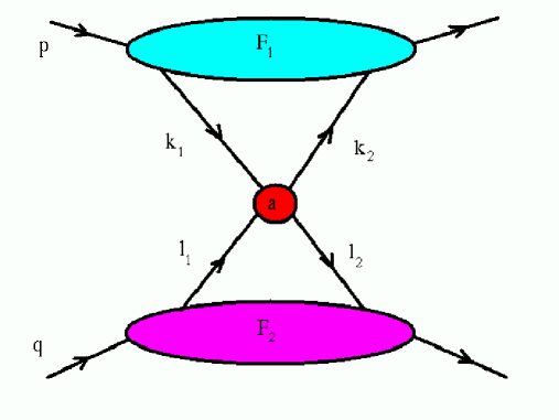
Refer to caption
FIG. 1.: Single scattering term
Refer to caption
FIG. 2.: Soft blob in the single scattering term.
Refer to caption
FIG. 3.: Double scattering term.
Refer to caption
FIG. 4.: Graphical representation of Eq.22.
Refer to caption
FIG. 5.: Double parton density in the case of direct coupling of the BFKL pomerons to the constinuent quarks.
Refer to caption
FIG. 6.: Double parton density in the triple pomeron case.