UT-STPD-3/00
FTUAM 00-09 Cold Dark Matter and $b\rightarrow s\gamma$ in the Hořava-Witten Theory

Abstract

The minimal supersymmetric standard model with complete, partial or no Yukawa unification and radiative electroweak breaking with boundary conditions from the Hořava-Witten theory is considered. The parameters are restricted by constraining the lightest sparticle relic abundance by cold dark matter considerations and requiring the $b$-quark mass after supersymmetric corrections and the branching ratio of $b\rightarrow s\gamma$ to be compatible with data. Complete Yukawa unification can be excluded. Also, $t-b$ Yukawa unification is strongly disfavored since it requires almost degenerate lightest and next-to-lightest sparticle masses. However, the $b-\tau$ or no Yukawa unification cases avoid this degeneracy. The latter with $\mu<0$ is the most natural case. The lightest sparticle mass, in this case, can be as low as about $77~{}{\rm GeV}$.

Recently, it has been realized that the five existing perturbative string theories (type I open strings, type IIA and IIB closed strings, and the $E_{8}\times E^{\prime}_{8}$ and $SO(32)$ closed heterotic strings) and the 11-dimensional supergravity correspond to different vacua of a unique underlying theory, called M-theory. Hořava and Witten have shown [1] that the strong coupling limit of the $E_{8}\times E^{\prime}_{8}$ heterotic string theory is equivalent to the low energy limit of M-theory compactified on $S^{1}/Z_{2}$ which is a line segment of length $\rho$. As $\rho\to 0$, the weakly coupled heterotic string is recovered. The observable $E_{8}$ gauge fields reside in one (10-dimensional) end of this segment, while the hidden sector $E^{\prime}_{8}$ gauge fields reside in its other end. Gravitational fields propagate in the 11-dimensional bulk.

The main success of the Hořava-Witten theory is that it solves, in an elegant way, the gauge coupling unification problem, i.e., the discrepancy between the supersymmetric (SUSY) grand unified theory (GUT) scale $M_{X}\simeq 2\times 10^{16}{\rm{GeV}}$ (consistent with the data on the low energy gauge coupling constants) and the string unification scale $M_{str}\simeq 5\times 10^{17}{\rm{GeV}}$ calculated in the weakly coupled string theory. Before M-theory, there were several proposals (such as large threshold corrections, intermediate scales, and extra particles) for explaining this discrepancy but none was totally satisfactory. In the strongly coupled heterotic string theory, the extra Kaluza-Klein states do not affect the running of the gauge coupling constants, which live on the boundary of the 11-dimensional spacetime. On the contrary, they accelerate the running of the gravitational coupling constant and, thus, reduce $M_{str}$ to $M_{X}$. Moreover, SUSY breaking in M-theory naturally leads [2] to gaugino masses of the order of the gravitino mass in contrast to the weakly coupled heterotic string case where the gaugino masses were tiny.

Similarly to the weakly coupled heterotic string, the compactification of the Hořava-Witten theory can lead to the spontaneous breaking of $E_{8}$ to phenomenologically more interesting groups. The simplest breaking of $E_{8}$ to $E_{6}$ is achieved [3] by the so-called standard embedding (SE), where the holonomy group of the spin connection of a Calabi-Yau three-fold is identified with a $SU(3)$ subgroup of $E_{8}$. Further breaking of $E_{6}$ to semi-simple groups such as the trinification group $SU(3)_{c}\times SU(3)_{L}\times SU(3)_{R}$ and the flipped $SU(6)\times U(1)$ group can be performed via Wilson loops. The trinification group contains $SU(2)_{R}$. Assuming then that the Higgs doublets and the third family right-handed quarks form $SU(2)_{R}$ doublets, one obtains [4] the ‘asymptotic’ Yukawa coupling relation $h_{t}=h_{b}$ and, hence, large $\tan\beta\approx m_{t}/m_{b}$. The flipped $SU(6)$, for certain embeddings of the minimal supersymmetric standard model (MSSM) fields, contains [5] $SU(4)_{c}$. Requiring that the third family lepton doublet belongs to $SU(6)$ 15-plets and the right-handed $b$-quark as well as the Higgs doublet coupling to the down-type quarks belong to $SU(6)$ $\bar{6}$-plets, one gets ‘asymptotic’ $b-\tau$ Yukawa unification ($h_{b}=h_{\tau}$).

In the strongly coupled case, the SE is not special [6]. Non-standard embeddings (NSE) may lead to simple gauge groups such as $SU(5)$ or $SO(10)$ which could yield $b-\tau$ or complete ($h_{t}=h_{b}=h_{\tau}$) Yukawa unification. However, in general, we do not obtain Higgs superfields in the adjoint representation. Further gauge symmetry breaking then requires Wilson loops and, thus, (partial) Yukawa unification is lost. This may be avoided by employing special constructions with higher Kac-Moody level [7]. Complete Yukawa unification can be obtained in the Pati-Salam gauge group $SU(4)_{c}\times SU(2)_{L}\times SU(2)_{R}$ which may arise in NSE. This group contains both $SU(4)_{c}$ and $SU(2)_{R}$ and does not require Wilson loops for its breaking. Furthermore, in string theories where the couplings have a common origin, partial or complete Yukawa unification can be realized even without a unified gauge group [8]. Thus all four possibilities with complete, partial ($t-b$ or $b-\tau$) or no Yukawa unification are in principle allowed.

The soft SUSY breaking in the SE and NSE cases has been studied in Ref.[9]. One obtains universal boundary conditions, i.e., a common scalar mass $m_{0}$, a common gaugino mass $M_{1/2}$ and a common trilinear coupling $A_{0}$ given by (with zero vacuum energy density and no CP violating phases)

$$m_{0}^{2}=m_{3/2}^{2}-\frac{3m_{3/2}^{2}}{(3+\epsilon)^{2}}\left(\epsilon(6+\epsilon)\sin^{2}\theta+(3+2\epsilon)\cos^{2}\theta-2\sqrt{3}\epsilon\cos\theta\sin\theta\right),$$ (1)

$$M_{1/2}=\frac{\sqrt{3}m_{3/2}}{1+\epsilon}(\sin\theta+\frac{\epsilon}{\sqrt{3}}\cos\theta),$$ (2)

$$A_{0}=-\frac{\sqrt{3}m_{3/2}}{3+\epsilon}\left((3-2\epsilon)\sin\theta+\sqrt{3}\epsilon\cos\theta\right),$$ (3)

where $m_{3/2}$ is the gravitino mass, $\theta$ ($0<\theta<\pi/2$) is the goldstino angle, and the parameter $\epsilon$ lies between 0 ($-1$) and 1 in the SE (NSE) case [9]. The range of $\epsilon$ is the only difference between the two embeddings at the level of soft SUSY breaking.

In this paper, we will study the MSSM which results from the Hořava-Witten theory. We will assume radiative electroweak symmetry breaking with the universal boundary conditions in Eqs.(1)-(3) and examine all cases with complete, partial ($t-b$ or $b-\tau$) or no Yukawa unification. Our main aim is to restrict the parameter space by simultaneously imposing a number of phenomenological and cosmological constraints. In particular, the $b$-quark mass after including SUSY corrections and the branching ratio of $b\rightarrow s\gamma$ should be compatible with data. Also, the lightest supersymmetric particle (LSP) is required to provide the cold dark matter (CDM) in the universe. Its relic abundance must then be consistent with either of the two available cosmological models with zero/nonzero cosmological constant, which provide the best fits to all the data (see Refs.[10, 11]).

The GUT scale $M_{X}$ and gauge coupling constant are determined by using the 2-loop SUSY renormalization group equations (RGEs) for the gauge and Yukawa coupling constants between $M_{X}$ and a common SUSY threshold $M_{S}\approx\sqrt{m_{\tilde{t}_{1}}m_{\tilde{t}_{2}}}$ ($\tilde{t}_{1,2}$ are the stop quark mass eigenstates), which minimizes the radiative corrections to $\mu$ and $m_{A}$ (see e.g., Ref.[12]). Between $M_{S}$ and $m_{Z}$, we take the standard model (SM) 1-loop RGEs. The $t$-quark and $\tau$-lepton masses are fixed to their central experimental values $m_{t}(m_{t})=166~{}{\rm{GeV}}$ and $m_{\tau}(m_{\tau})=1.78~{}{\rm{GeV}}$. The asymptotic values of $h_{t}$, $h_{\tau}$ are then determined for each $\tan\beta$ at $M_{S}$ and $h_{b}$ is derived from $t-b$ or $b-\tau$ Yukawa unification. The resulting $m_{b}(m_{Z})$ is compared to its experimental value $m_{b}(m_{Z})\simeq 2.67\pm 0.98~{}{\rm{GeV}}$ [13] (with a $95\%$ confidence margin) after 1-loop SUSY corrections. For complete Yukawa unification, $\tan\beta$ at $M_{S}$ is fixed. For no Yukawa unification, $h_{b}$ is adjusted so that the corrected $m_{b}(m_{Z})=2.67~{}{\rm{GeV}}$. $M_{S}$ is specified consistently with the SUSY spectrum.

We next integrate the 1-loop RGEs for the soft SUSY breaking terms assuming universal boundary conditions given by Eqs.(1)-(3). At $M_{S}$, we impose the minimization conditions to the tree-level renormalization group improved potential and calculate the Higgsino mass $\mu$ (up to its sign). The sparticle spectrum is evaluated at $M_{S}$. The LSP, which is the lightest neutralino ($\tilde{\chi}$), turns out to be bino-like with purity $>98\%$ for almost all values of the parameters. The next-to-lightest supersymmetric particle (NLSP) is the lightest stau ($\tilde{\tau}_{2}$). Since we consider large $\tan\beta$’s too, we are obliged to include the third generation sfermion mixing. The mixing of the lighter generation sfermions, however, remains negligible due to the small masses of the corresponding fermions. Furthermore, we take into account the 2-loop radiative corrections [14] to the CP-even neutral Higgs boson masses $m_{h}$, $m_{H}$, which turn out to be sizeable for the lightest boson $h$.

Our calculation depends on the following free parameters: ${\rm sign}\mu$, $\tan\beta$, $m_{3/2}$, $\epsilon$, $\theta$. The relation found in Ref.[15] between the CP-odd Higgs boson mass $m_{A}$ and the asymptotic scalar and gaugino masses, takes, in our case, the form

$$m^{2}_{A}\simeq c_{3/2}m_{3/2}^{2}+c_{s}m_{3/2}^{2}\sin^{2}\theta+c_{2s}m_{3/2}^{2}\sin{2\theta}-m_{Z}^{2}~{},$$ (4)

where the coefficients $c_{3/2}\sim 0.1$, $c_{s},c_{2s}\sim 1$ depend on $\tan\beta$, $\epsilon$, and $M_{S}$. We verified that this relation holds with an accuracy better than $0.02\%$. We use it to express $m_{3/2}$ in terms of $m_{A}$ for fixed ${\rm sign}\mu$, $\tan\beta$, $\epsilon$ and $\theta$ ($M_{S}$ is determined self-consistently from the SUSY spectrum). The free parameter $m_{3/2}$ can, thus, be replaced by $m_{A}$.

In practice, the number of free parameters can be reduced by one. To see this, we fix ${\rm sign}\mu$, $\tan\beta$ and $m_{A}$ and observe that, along the lines in the $\epsilon-\theta$ plane where $m_{0}$ and $M_{1/2}$ remain constant, $A_{0}$ varies only by a few per cent. Consequently, the whole sparticle spectrum (except the gravitino mass) remains essentially unchanged along these lines which we call equispectral lines. Thus, for all practical purposes, $\epsilon$ and $\theta$ can be replaced by a single parameter which we choose to be the relative mass splitting between the LSP and the NLSP $\Delta_{NLSP}=(m_{\tilde{\tau}_{2}}-m_{\tilde{\chi}})/m_{\tilde{\chi}}$. Our final free parameters then are ${\rm sign}\mu$, $\tan\beta$, $m_{A}$, $\Delta_{NLSP}$. Note that, for fixed $\epsilon$, $\Delta_{NLSP}$ increases as $\theta$ decreases. Also, for fixed $\theta>\pi/6~{}(<\pi/6)$, $\Delta_{NLSP}$ decreases (increases) as $\epsilon$ increases. Finally, we find that $\Delta_{NLSP}$ is maximized, generally, at $\theta=\pi/9$ and $\epsilon\to 1$. Our calculation is performed at an appropriate value of $\epsilon$ in each case so that all relevant $\Delta_{NLSP}$’s can be obtained.

An important constraint results from the inclusive branching ratio of $b\rightarrow s\gamma$ [16], which is calculated here by using the formalism of Ref.[17]. The dominant contributions, besides the SM one, come from the charged Higgs bosons ($H^{\pm}$) and the charginos. The former interferes constructively with the SM contribution, while the latter interferes constructively (destructively) with the other two contributions when $\mu>0$ ($\mu<0$). The SM contribution, which is factorized out in the formalism of Ref.[17], includes the next-to-leading order (NLO) QCD [18] and the leading order (LO) QED [17, 19] corrections. The NLO QCD corrections [20] to the charged Higgs boson contribution are taken from the first paper in Ref.[20]. The SUSY contribution is evaluated by including only the LO QCQ corrections using the formulae in Ref.[21]. NLO QCD corrections to the SUSY contribution have also been discussed in Ref.[21], but only under certain very restrictive conditions which never hold in our case since the chargino and lightest stop quark masses are comparable to the masses of the other squarks and the gluinos. We, thus, do not include these corrections in our calculation.

The branching ratio ${\rm BR}(b\rightarrow s\gamma)$ is first evaluated with central values of the input parameters and the renormalization and matching scales. We find that, for each ${\rm sign}\mu$, $\tan\beta$ and $\Delta_{NLSP}$, there exists a value of $m_{A}$ above which the ${\rm BR}(b\rightarrow s\gamma)$ enters and remains in the experimentally allowed region [22]: $2\times 10^{-4}\stackrel{{{}_{<}}}{{{}_{\sim}}}{\rm BR}(b\rightarrow s\gamma)\stackrel{{{}_{<}}}{{{}_{\sim}}}4.5\times 10^{-4}$. This lower bound on $m_{A}$ corresponds to the upper (lower) bound on the branching ratio for $\mu>0$ ($\mu<0$) and, for most of the parameter space, is its absolute minimum. For relatively small $\tan\beta$’s, however, the absolute minimum of $m_{A}$ comes from the experimental bound $m_{h}\stackrel{{{}_{>}}}{{{}_{\sim}}}113.4~{}{\rm GeV}$. We take $\tan\beta\gtrsim 2.3$ since otherwise $m_{h}$ is too small.

The lower bound on $m_{A}$ can be considerably reduced if the theoretical uncertainties entering into the calculation of ${\rm BR}(b\rightarrow s\gamma)$ are taken into account. These uncertainties originating from the experimental errors in the input parameters and the ambiguities in the renormalization and matching scales are known to be quite significant. The SM and charged Higgs contributions generate an uncertainty of about $\pm 10\%$ (see first paper in Ref.[20]). The uncertainty from the SUSY contribution cannot be reliably calculated at the moment since the NLO QCD corrections to this contribution are not known in our case. Fortunately, the SUSY contribution is pretty small in all cases which are crucial for our qualitative conclusions. Be that as it may, we take the uncertainty from this contribution, evaluated at the LO in QCD, to be about $\pm 30\%$.

For large or intermediate $\tan\beta$’s, a severe restriction arises from the sizable SUSY corrections to the $b$-quark mass. The dominant contributions are from the sbottom-gluino and stop-chargino loops and are calculated by using the simplified formulae of Ref.[23]. We find here that the size of these corrections practically depends only on $\tan\beta$ (compare with Refs.[12, 15]). Also, their sign is opposite to the one of $\mu$ in contrast to the chargino contribution to the ${\rm BR}(b\rightarrow s\gamma)$ which, as mentioned, has the sign of $\mu$.

An additional restriction comes from the LSP cosmic relic abundance. We calculate this abundance by closely following the formalism of Ref.[10] where $\tilde{\chi}-\tilde{\tau}_{2}$ coannihilations [24] have been consistently included for all values of $\tan\beta$. However, coannihilations [25] of these sparticles with the lighter generation right-handed sleptons $\tilde{e}_{R}$, $\tilde{e}_{R}^{\ast}$, $\tilde{\mu}_{R}$, $\tilde{\mu}_{R}^{\ast}$ (considered degenerate), which were ignored in Ref.[10], are now important and must be included since our calculation here extends to small ($\lesssim 15$) $\tan\beta$’s too [24]. The effective cross section entering into the Boltzmann equation then becomes

$$\sigma_{eff} = \sigma_{\tilde{\chi}\tilde{\chi}}r_{\tilde{\chi}}r_{\tilde{\chi}}+4\sigma_{\tilde{\chi}\tilde{\tau}_{2}}r_{\tilde{\chi}}r_{\tilde{\tau}_{2}}+2(\sigma_{\tilde{\tau}_{2}\tilde{\tau}_{2}}+\sigma_{\tilde{\tau}_{2}\tilde{\tau}_{2}^{\ast}})r_{\tilde{\tau}_{2}}r_{\tilde{\tau}_{2}}+8(\sigma_{\tilde{\tau}_{2}\tilde{e}_{R}}+\sigma_{\tilde{\tau}_{2}\tilde{e}_{R}^{\ast}})r_{\tilde{\tau}_{2}}r_{\tilde{e}_{R}}$$ (5)

$$+ 8\sigma_{\tilde{\chi}\tilde{e}_{R}}r_{\tilde{\chi}}r_{\tilde{e}_{R}}+4(\sigma_{\tilde{e}_{R}\tilde{e}_{R}}+\sigma_{\tilde{e}_{R}\tilde{e}_{R}^{\ast}})r_{\tilde{e}_{R}}r_{\tilde{e}_{R}}+4(\sigma_{\tilde{e}_{R}\tilde{\mu}_{R}}+\sigma_{\tilde{e}_{R}\tilde{\mu}_{R}^{\ast}})r_{\tilde{e}_{R}}r_{\tilde{e}_{R}}.$$ (6)

Here $\sigma_{ij}$ ($i,j=\tilde{\chi}$, $\tilde{\tau}_{2}$, $\tilde{\tau}_{2}^{\ast}$, $\tilde{e}_{R}$, $\tilde{e}_{R}^{\ast}$, $\tilde{\mu}_{R}$, $\tilde{\mu}_{R}^{\ast}$) is the total cross section for particle $i$ to annihilate with particle $j$ averaged over initial spin and particle-antiparticle states and the $r_{i}$’s can be found from Ref.[10]. The Feynman graphs for $\sigma_{\tilde{\chi}\tilde{\chi}}$, $\sigma_{\tilde{\chi}\tilde{\tau}_{2}}$, $\sigma_{\tilde{\tau}_{2}\tilde{\tau}_{2}}$, and $\sigma_{\tilde{\tau}_{2}\tilde{\tau}_{2}^{\ast}}$ are listed in Table I of Ref.[10]. From these diagrams, we can also obtain the ones for $\sigma_{\tilde{\chi}\tilde{e}_{R}}$, $\sigma_{\tilde{e}_{R}\tilde{e}_{R}}$, $\sigma_{\tilde{e}_{R}\tilde{e}_{R}^{\ast}}$ by replacing $\tilde{\tau}_{2}$ by $\tilde{e}_{R}$ and $\tau$ by $e$ and ignoring diagrams with $\tilde{\tau}_{1}$ exchange. The processes $\tilde{\tau}_{2}\tilde{e}_{R}\rightarrow\tau e$, $\tilde{\tau}_{2}\tilde{e}_{R}^{\ast}\rightarrow\tau\bar{e}$, $\tilde{e}_{R}\tilde{\mu}_{R}\rightarrow e\mu$ and $\tilde{e}_{R}\tilde{\mu}_{R}^{\ast}\rightarrow e\bar{\mu}$ are realized via a t-channel $\tilde{\chi}$ exchange. The calculation of the $a_{ij}$’s and $b_{ij}$’s given in Ref.[10] is readily extended to include these extra processes too.

The main contribution to the LSP (almost pure bino) annihilation cross section generally arises from stau exchange in the t- and u-channel leading to $\tau\bar{\tau}$ in the final state. We do not include s-channel exchange diagrams. So our results are not valid for values of $m_{\tilde{\chi}}$ very close to the poles at $m_{Z}/2$, $m_{h}/2$, $m_{H}/2$ or $m_{A}/2$ where the annihilation cross section is enhanced and the relic density drops considerably. The expressions for $a_{\tilde{\chi}\tilde{\chi}}$ and $b_{\tilde{\chi}\tilde{\chi}}$ can be found in Ref.[10] (with the final state lepton masses neglected).

The most important contribution to coannihilation arises from the $a_{ij}$’s. (The contribution of the $b_{ij}$’s ($ij\neq\tilde{\chi}\tilde{\chi}$), although included in the calculation, is in general negligible.) The contributions of the various coannihilation processes to the $a_{ij}$’s and $b_{ij}$’s ($ij\neq\tilde{\chi}\tilde{\chi}$) are calculated using techniques and approximations similar to the ones in Ref.[10]. In particular, the contributions to the $a_{ij}$’s from the processes with

• $\tilde{\chi}\tilde{\tau}_{2}$, $\tilde{\tau}_{2}\tilde{\tau}_{2}$, $\tilde{\tau}_{2}\tilde{\tau}_{2}^{\ast}$ in the initial state are listed in Table II of Ref.[10].

• $\tilde{\chi}\tilde{e}_{R}$, $\tilde{e}_{R}\tilde{e}_{R}^{\ast}$ in the initial state can be obtained from the formulae in Tables II and IV of Ref.[10] by the replacement $\tilde{\tau}_{2}\rightarrow\tilde{e}_{R}$ and putting $\theta=0$, $m_{\tau}=0$.

• $\tilde{\tau}_{2}\tilde{e}_{R}$, $\tilde{\tau}_{2}\tilde{e}_{R}^{\ast}$, $\tilde{e}_{R}\tilde{e}_{R}$, $\tilde{e}_{R}\tilde{\mu}_{R}$, $\tilde{e}_{R}\tilde{\mu}_{R}^{\ast}$ in the initial state are listed in the following Table:

  TABLE. Contributions to the Coefficients $a_{ij}$

  Process	Contribution to the Coefficient $a_{ij}$
  $\tilde{\tau}_{2}\tilde{e}_{R}\rightarrow\tau e$	$e^{4}Y_{R}^{4}\cos^{2}\theta m_{\tilde{\chi}}^{2}(m_{\tilde{e}_{R}}+m_{\tilde{\tau}_{2}})^{2}/$
  	$8\pi c_{W}^{4}m_{\tilde{e}_{R}}m_{\tilde{\tau}_{2}}(m_{\tilde{\chi}}^{2}+m_{\tilde{e}_{R}}m_{\tilde{\tau}_{2}})$
  $\tilde{\tau}_{2}\tilde{e}_{R}^{\ast}\rightarrow\tau\bar{e}$	$e^{4}Y_{L}^{2}Y_{R}^{2}\sin^{2}\theta m_{\tilde{\chi}}^{2}(m_{\tilde{e}_{R}}+m_{\tilde{\tau}_{2}})^{2}/$
  	$8\pi c_{W}^{4}m_{\tilde{e}_{R}}m_{\tilde{\tau}_{2}}(m_{\tilde{\chi}}^{2}+m_{\tilde{e}_{R}}m_{\tilde{\tau}_{2}})$
  $\tilde{e}_{R}\tilde{e}_{R}\rightarrow ee$	$e^{4}Y_{R}^{4}m_{\tilde{\chi}}^{2}/\pi c_{W}^{4}\Sigma_{e}^{2}$
  $\tilde{e}_{R}\tilde{\mu}_{R}\rightarrow e\mu$	$e^{4}Y_{R}^{4}m_{\tilde{\chi}}^{2}/2\pi c_{W}^{4}\Sigma_{e}^{2}$
  $\tilde{e}_{R}\tilde{\mu}_{R}^{\ast}\rightarrow e\bar{\mu}$	$e^{4}Y_{R}^{4}m_{\tilde{e}_{R}}^{2}/12\pi c_{W}^{4}\Sigma_{e}^{2}$

  where $\theta$ is the stau mixing angle (not to be confused with the goldstino angle), $c_{W}=\cos\theta_{W}$, $Y_{L(R)}=-1/2(-1)$ is the hypercharge of the left(right)-handed leptons and $\Sigma_{e}=m_{\tilde{\chi}}^{2}+m_{\tilde{e}_{R}}^{2}$ with $m_{\tilde{e}_{R}}$ being the common mass of $\tilde{e}_{R}$, $\tilde{\mu}_{R}$.

The LSP relic abundance $\Omega_{LSP}~{}h^{2}$, which remains practically constant on the equispectral lines, can now be evaluated for any ${\rm sign}\mu$, $\tan\beta$, $m_{A}$ and $\Delta_{NLSP}$. We find that, away from the poles, $\Omega_{LSP}~{}h^{2}$ increases with $m_{A}$ (or $m_{\tilde{\chi}}$). Also, for fixed $m_{\tilde{\chi}}$, it increases with $\Delta_{NLSP}$, since coannihilation becomes less efficient. The mixed or the pure cold (in the presence of a nonzero cosmological constant) dark matter scenarios for large scale structure formation require $0.09\stackrel{{{}_{<}}}{{{}_{\sim}}}\Omega_{LSP}~{}h^{2}\stackrel{{{}_{<}}}{{{}_{\sim}}}0.22$ [10, 11], which restricts $\Delta_{NLSP}$ .

We will first examine the case with no Yukawa unification. As already mentioned, the asymptotic value of $h_{b}$ is specified, in this case, by requiring that $m_{b}(m_{Z})$, after SUSY corrections, coincides with its central experimental value. For $\mu>0$, $m_{A}$ (and, thus, $m_{\tilde{\chi}}$) is forced to be quite large in order to have the ${\rm BR}(b\rightarrow s\gamma)$ reduced below its upper experimental limit. Thus, the LSP and NLSP masses are required to be relatively close to each other so that coannihilation is more efficient and the bounds on $\Omega_{LSP}~{}h^{2}$ can be satisfied. For $\mu<0$, smaller $m_{A}$’s are needed for enhancing the $b\rightarrow s\gamma$ branching ratio so as to overtake its lower bound. Thus, in some regions of the parameter space, one can get cosmologically acceptable LSP relic densities even without invoking coannihilation. For $\mu>0$, $\tan\beta\lesssim 38$ or $\mu<0$, the Higgs sector turns out to be heavier than the LSP and NLSP ($m_{A}\gtrsim 450~{}\{400\}~{}{\rm GeV}$ for $\mu>0$, $\tan\beta\lesssim 38$ and $m_{A}\gtrsim 340~{}\{310\}~{}{\rm GeV}$ for $\mu<0$) implying that processes with $\tau H$, $\tau A$, $hH$, $HH$, $H^{+}H^{-}$, $AA$ in the final state are, generally, kinematically blocked. Here and below, the limiting values obtained by including the theoretical uncertainty in ${\rm BR}(b\rightarrow s\gamma)$ are indicated in curly brackets.

We start by constructing the regions in the $m_{\tilde{\chi}}-\Delta_{NLSP}$ plane allowed by the CDM and $b\rightarrow s\gamma$ considerations for each ${\rm sign}\mu$ and $\tan\beta$. A typical example of such a region is shown in Fig.1 and corresponds to $\mu>0$ and $\tan\beta\simeq 10$. Here, we fixed $\epsilon=0.65$ and regulated $\Delta_{NLSP}$ via $\theta$. The lower bound on $m_{\tilde{\chi}}$ (almost vertical line) comes from the upper bound ($\simeq 4.5\times 10^{-4}$) on ${\rm BR}(b\rightarrow s\gamma)$. The lower (upper) curved boundary of the allowed region corresponds to $\Omega_{LSP}~{}h^{2}\simeq 0.09~{}(0.22)$ and the horizontal boundary to $\Delta_{NLSP}=0$. The maximal $m_{\tilde{\chi}}$ ($\Delta_{NLSP}$) is obtained at the lower right (upper left) corner of this region. The value of $m_{\tilde{\chi}}$ can vary between about $169~{}\{123\}$ and $575~{}{\rm GeV}$. So, the LSP is relatively heavy and the maximal allowed $\Delta_{NLSP}$ is small ($\simeq 0.096~{}\{0.19\}$). Coannihilation is important in the whole allowed region. On the contrary, for $\mu<0$ and $\tan\beta\simeq 10$, we find lighter LSPs. Specifically, $m_{\tilde{\chi}}$ varies between about $85~{}\{79\}$ and $572~{}{\rm GeV}$. So, the maximal allowed $\Delta_{NLSP}$ is much larger ($\simeq 0.6~{}\{0.71\}$) now, and there is a region ($85~{}\{79\}~{}{\rm GeV}\lesssim m_{\tilde{\chi}}\lesssim 120~{}{\rm GeV}$) where coannihilation is negligible. The lower bound on $m_{\tilde{\chi}}$, for $\mu<0$, corresponds to the lower bound on ${\rm BR}(b\rightarrow s\gamma)$ or $m_{h}$.

For $\mu<0$, there exist $\tan\beta$’s where the maximal $\Delta_{NLSP}$ is not obtained at the minimal $m_{\tilde{\chi}}$. This is illustrated in Fig.2 depicting the allowed region in the $m_{\tilde{\chi}}-\Delta_{NLSP}$ plane for $\mu<0$ and $\tan\beta\simeq 35.3$. Here, we fixed $\epsilon=0.99$. The LSP mass can vary between about $203$ and $614~{}{\rm GeV}$ with the lower bound corresponding to the lower bound on ${\rm BR}(b\rightarrow s\gamma)$. For the minimal $m_{\tilde{\chi}}$, the maximal $\Delta_{NLSP}$ ($\simeq 0.045$) does not correspond to $\Omega_{LSP}~{}h^{2}\simeq 0.22$. It is, rather, the absolute maximum of $\Delta_{NLSP}$ for the given values of ${\rm sign\mu}$, $\tan\beta$ and $m_{A}$ which is obtained at $\theta=\pi/9$ as indicated earlier and corresponds to $\Omega_{LSP}~{}h^{2}\simeq 0.114$. Increasing $m_{\tilde{\chi}}$, this absolute maximum of $\Delta_{NLSP}$ increases (along the inclined part of the left boundary) and $\Omega_{LSP}~{}h^{2}$ becomes $\simeq 0.22$ at $\Delta_{NLSP}\simeq 0.064$, which is the overall maximal allowed $\Delta_{NLSP}$ in this case. Including the theoretical uncertainty in ${\rm BR}(b\rightarrow s\gamma)$, we see that the vertical part of the boundary disappears and the minimal value of $m_{\tilde{\chi}}$ is reduced to about $198~{}{\rm{GeV}}$ corresponding to $\Delta_{NLSP}\simeq 0.038$.

The maximal allowed $\Delta_{NLSP}$’s can be found for all possible $\tan\beta$’s and any sign of $\mu$ by repeating the above analysis. The results are displayed in Fig.3, which shows the allowed regions in the $\tan\beta-\Delta_{NLSP}$ plane for $\mu>0$ (between the solid and dashed lines) and $\mu<0$ (between the solid and dot-dashed lines). Here, the bold (faint) lines are obtained by ignoring (including) the theoretical errors in ${\rm BR}(b\rightarrow s\gamma)$, and $\epsilon$ is chosen for each ${\rm sign}\mu$ and $\tan\beta$ so that it lies in the domain of all relevant equispectral lines. We found that $\Delta_{NLSP}=0$ can be achieved at the maximal LSP mass ($\sim 600-700~{}{\rm GeV}$) corresponding to each $\tan\beta$ between 2.3 and $43.9~{}\{44.3\}$. So, the minimal allowed $\Delta_{NLSP}$ is always zero. Regarding the maximal allowed $\Delta_{NLSP}$’s, we can distinguish the cases:

• For $\mu>0$ ($<0$) and $6.5~{}\{8.6\}~{}(9.2)\lesssim\tan\beta\lesssim 43.9~{}\{44.3\}~{}(34.5)$, the maximal $\Delta_{NLSP}$ corresponds to the lower bound on $m_{\tilde{\chi}}$ found from the experimental limits on ${\rm BR}(b\rightarrow s\gamma)$. The allowed regions are of the type in Fig.1 and the upper curves in Fig.3 are obtained from the upper left corners of these regions as we vary $\tan\beta$. For $\mu>0$, the lower curved boundary of the allowed regions disappears at high enough $\tan\beta$’s and, eventually, at $\tan\beta\simeq 43.9~{}\{44.3\}$, the allowed region shrinks to a point with $m_{\tilde{\chi}}\simeq 730~{}\{740\}~{}{\rm GeV}$ and $\Delta_{NLSP}\simeq 0$.

• For $\mu>0$ ($<0$) and $2.3\lesssim\tan\beta\lesssim 6.5~{}\{8.6\}~{}(9.2~{}\{9.8\})$, the lower bound on $m_{\tilde{\chi}}$ is found from the experimental limit on $m_{h}$. This mass comes out too small for small $m_{A}$’s. So, bigger $m_{A}$’s (and, thus, $m_{\tilde{\chi}}$’s) are required to raise $m_{h}$ above $113.4~{}{\rm GeV}$. The allowed regions are again typically as in Fig.1 (with or without the curved lower boundary) and the maximal $\Delta_{NLSP}$ rapidly decreases with $\tan\beta$.

• For $\mu<0$ and $\tan\beta$ between about $34.5~{}\{9.8\}$ and 41, the maximal $\Delta_{NLSP}$ does not correspond to the minimal $m_{\tilde{\chi}}$ from the lower limit on ${\rm BR}(b\rightarrow s\gamma)$ or $m_{h}$. The obtained allowed regions are of the type in Fig.2 (with or without the vertical part of the boundary). As $\tan\beta$ increases above $34.5~{}\{9.8\}$, the inclined part of their left boundary moves to the right and the vertical part eventually disappears. At even higher $\tan\beta$’s, the curved lower boundary also disappears and, finally, the region shrinks to a point at $\tan\beta\simeq 41$ with $\Delta_{NLSP}\simeq 0$ and $m_{\tilde{\chi}}\simeq 640~{}{\rm GeV}$. For low $\tan\beta$’s, the bino purity of the LSP decreases from above $98\%$ to $95\%$ and our calculation, which assumes a bino-like LSP, becomes less accurate.

In conclusion, in the case of no Yukawa unification and for $\mu>0$ ($<0$), the maximal $\Delta_{NLSP}\approx 0.16~{}\{0.25\}~{}(0.68~{}\{0.73\})$ is achieved at $\tan\beta\approx 6.5~{}\{8.6\}~{}(9.2~{}\{9.8\})$. Also, $138~{}\{114\}~{}(84~{}\{77\})~{}{\rm GeV}\lesssim m_{\tilde{\chi}}\lesssim 730~{}\{740\}~{}(640)~{}{\rm GeV}$. The minimal $m_{\tilde{\chi}}$ corresponds to the maximal $\Delta_{NLSP}$ except $m_{\tilde{\chi}}\approx 77~{}{\rm GeV}$ which is obtained at $\tan\beta\approx 20.4$.

We now turn to the case of $b-\tau$ Yukawa unification. To keep $\tilde{\tau}_{2}$ heavier than $\tilde{\chi}$, we must take $\tan\beta\lesssim 45$. For $\mu<0$, the values of $m_{b}(m_{Z})$, obtained from this unification assumption, turn out to be larger than the experimental upper limit [13] after including the SUSY corrections. This forces us to take $\mu>0$. In Fig.4, we plot the tree-level (dotted line) and the corrected (solid line) $m_{b}(m_{Z})$ versus $\tan\beta$ for $\Delta_{NLSP}\simeq 0$ and the minimal value of $m_{A}$ which corresponds to ${\rm BR}(b\rightarrow s\gamma)\simeq 4.5\times 10^{-4}$ for $6.5\lesssim\tan\beta\lesssim 45$ or $m_{h}\approx 113.4~{}{\rm GeV}$ for $2.3\lesssim\tan\beta\lesssim 6.5$. This choice is not crucial, because $m_{b}(m_{Z})$, for fixed $\tan\beta$, turns out to be almost independent from $m_{A}$ and $\Delta_{NLSP}$. The corrected $m_{b}(m_{Z})$ increase as $\tan\beta$ decreases and reaches a maximum of about $3.65~{}{\rm GeV}$ at $\tan\beta\approx 4.7$. The SUSY corrections decrease with $\tan\beta$. We find that, in the entire range $2.3\lesssim\tan\beta\lesssim 45$, the corrected $m_{b}(m_{Z})$ is within the experimental limits.

Due to the relatively heavy LSP obtained with $\mu>0$, coannihilation is generally important for reducing $\Omega_{LSP}~{}h^{2}$ to an acceptable level. For $38\lesssim\tan\beta\lesssim 45$, the maximal allowed $m_{LSP}$ is raised to $\approx 790~{}{\rm GeV}$ due to the fact that the processes with $\tau H$, $\tau A$ in the final state are kinematically allowed. Thus, coannihilation is strengthened and larger $m_{LSP}$’s are allowed. On the contrary, for $2.3\lesssim\tan\beta\lesssim 34$, these processes are blocked and the upper bound on $m_{LSP}$ decreases to $\approx 580~{}{\rm GeV}$. $\Delta_{NLSP}$ ranges between 0 and $\approx 0.16~{}\{0.25\}$ with its maximum achieved at $\tan\beta\approx 6.5~{}\{8.6\}$ corresponding to the lowest possible $m_{LSP}\approx 141~{}\{115\}~{}{\rm GeV}$. Finally, in the range $34\lesssim\tan\beta\lesssim 38$, $m_{LSP}$ can get close to $m_{A}/2$, $m_{H}/2$ for certain $m_{A}$’s and $\Omega_{LSP}~{}h^{2}$ can be considerably reduced. Thus, the maximal $\Delta_{NLSP}$ and $m_{LSP}$ can be very large in isolated regions of the parameter space. This also applies in the no Yukawa unification case with $\mu>0$.

In the case of $t-b$ Yukawa unification the corrected $m_{b}(m_{Z})$, for $\mu<0$, again turns out to be larger than the experimental upper limit, so we must still choose $\mu>0$. We find that, for $34.3\lesssim\tan\beta$, the corrected $m_{b}(m_{Z})$ is compatible with the experimental limits after including its theoretical uncertainties ($\approx 6\%$). This provides the lower bound on $\tan\beta$ if the theoretical uncertainties in ${\rm BR}(b\rightarrow s\gamma)$ are included. Without these uncertainties, however, the lower bound on $\tan\beta$ is 43.7 below which the allowed region in the $m_{LSP}-\Delta_{NLSP}$ plane disappears. To keep $\tilde{\tau}_{2}$ heavier than $\tilde{\chi}$, we must take $\tan\beta\lesssim 48.5$. So there is an allowed range $43.7~{}\{33.5\}\lesssim\tan\beta\lesssim 48.5$ in which the minimal $m_{LSP}$ is about $730~{}\{507\}~{}{\rm GeV}$ with the maximal $\Delta_{NLSP}$ being $\approx 0~{}\{0.01\}$.

For complete Yukawa unification, the lightest stau turns out to be lighter than the neutralino (by at least $11\%$). So, this case is excluded.

Theoretical errors from the implementation of the radiative electroweak breaking, the renormalization group analysis and the radiative corrections to (s)particle masses, and inclusion of experimental margins of various quantities can only further widen the allowed parameter ranges which we obtained. They will also produce a larger uncertainty in Eq.(4). However, all these ambiguities are not expected to change our qualitative conclusions, especially the exclusion of complete Yukawa unification.

Neutralinos could be detected via their elastic scattering with nuclei. For an almost pure bino, however, the cross section is expected to lie well below the reported sensitivity [$(1-10)\times 10^{-6}~{}\rm{Pb}$] of current experiments (DAMA). The reason is that the channels with Higgs and $Z$ boson (squark) exchange are suppressed (by the squark mass).

In summary, we studied the MSSM with radiative electroweak breaking and boundary conditions from the Hořava-Witten theory. We assumed complete, partial or no Yukawa unification. The parameters were restricted by assuming that the CDM consists of the LSP and requiring $m_{b}$, after SUSY corrections, and ${\rm BR}(b\rightarrow s\gamma$) to be compatible with data. We found that complete Yukawa unification is excluded. Also, $t-b$ Yukawa unification is strongly disfavored since it requires the LSP and NLSP masses to be almost degenerate. This can be avoided with $b-\tau$ or no Yukawa unification which, for $\mu<0$, is the most natural case and allows the LSP mass to be as low as $\approx 77~{}{\rm GeV}$.

We thank M. Gómez and C. Muñoz for discussions. S. K. is supported by the Spanish Ministerio de Educacion y Cultura and C. P. by the Greek State Scholarship Institution (I. K. Y.). This work was supported by the EU under TMR contract No. ERBFMRX–CT96–0090 and the Greek Government research grant PENED/95 K.A.1795.

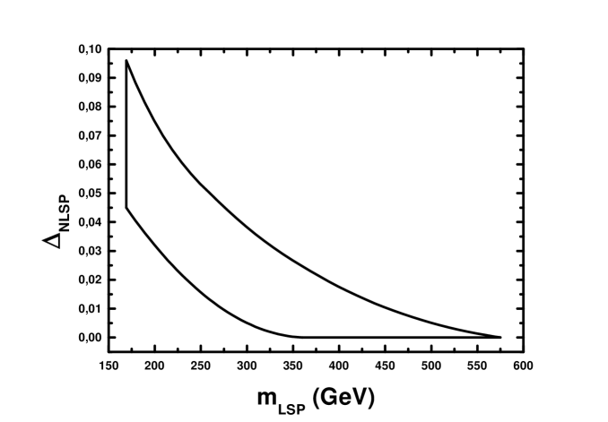
FIG. 1.: The allowed region in the $m_{LSP}-\Delta_{NLSP}$ plane for $\mu>0$ and $\tan\beta\simeq 10$ ($\epsilon=0.65$). ${\rm{BR}}(b\rightarrow s\gamma)$ is evaluated with central values of the input parameters and scales.

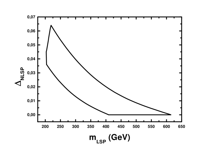
FIG. 2.: The allowed region in the $m_{LSP}-\Delta_{NLSP}$ plane for $\mu<0$, $\tan\beta\simeq 35.3$ ($\epsilon=0.99$). ${\rm{BR}}(b\rightarrow s\gamma)$ is evaluated with central values of the input parameters and scales.

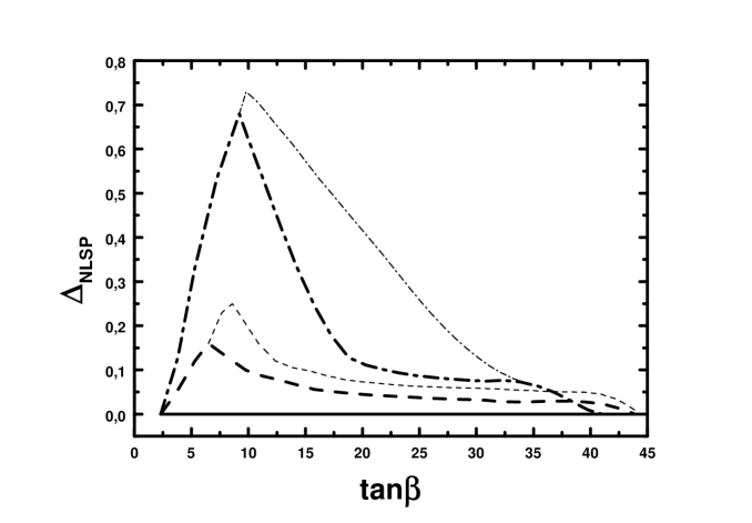
FIG. 3.: The allowed region in the $\tan\beta-\Delta_{NLSP}$ plane for $\mu>0~{}(<0)$ is between the solid and (dot-)dashed lines. The bold (faint) lines are without (with) the errors in ${\rm BR}(b\rightarrow s\gamma)$.

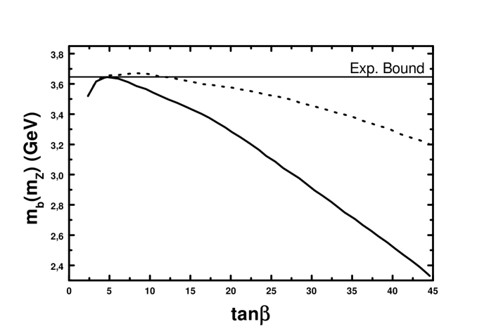
FIG. 4.: The tree-level (dotted line) and the corrected (solid line) $m_{b}(m_{Z})$ versus $\tan\beta$ for $\Delta_{NLSP}\simeq 0$ and the minimal $m_{A}$. The experimental upper bound on $m_{b}(m_{Z})$ is shown too.

REFERENCES

- [1] P. Hořava and E. Witten, Nucl. Phys. B460 (1996) 506; ibid. 475 (1996) 94.
- [2] H. P. Nilles, M. Olechochowski and M. Yamaguchi, Phys. Lett. B415 (1997) 24.
- [3] E. Witten, Nucl. Phys. B471 (1996) 195.
- [4] G. Lazarides and C. Panagiotakopoulos, Phys. Lett. B337 (1994) 90.
- [5] C. Panagiotakopoulos, Int. Jour. Mod. Phys. A5 (1990) 2359.
- [6] A. Lukas, B. A. Ovrut and D. Waldram, JHEP 9906 (1999) 034.
- [7] G. Aldazabal, G. A. Font, L. E. Ibáñez and A. Uranga, Nucl. Phys. B452 (1995) 3; ibid. 465 (1996) 34.
- [8] S. Khalil and T. Kobayashi, Nucl. Phys. B526 (1998) 99.
- [9] T. Kobayashi, J. Kubo and H. Shimabukuro, Nucl. Phys. B580 (2000) 3; D. G. Cerdeño and C. Muñoz, Phys. Rev. D61 (2000) 016001.
- [10] M. Gómez, G. Lazarides and C. Pallis, Phys. Rev. D61 (2000) 123512.
- [11] A. B. Lahanas, D. V. Nanopoulos and V. C. Spanos, Phys. Lett. B464 (1999) 213.
- [12] M. Gómez, G. Lazarides and C.Pallis, Phys. Lett. B487 (2000) 313.
- [13] S. Martí i Gracía, J. Fuster and S. Cabrera, Nucl. Phys. (Proc. Sup.) B64 (1998) 376.
- [14] S. Heinemeyer, W. Hollik and G. Weiglein, hep-ph/0002213.
- [15] M.Carena, M.Olechowski, S.Pokorski and C.Wagner, Nucl. Phys. B426 (1994) 269.
- [16] S. Bertolini, F. Borzumati, A. Masiero and G. Ridolfi, Nucl. Phys. B353 (1991) 591; R. Barbieri and G. F. Giudice, Phys. Lett. B309 (1993) 86.
- [17] A. L. Kagan and M. Neubert, Eur. Phys. J. C7 (1999) 5.
- [18] A. Ali and C. Greub, Z. Phys. C49 (1991) 431; Phys. Lett. B259 (1991) 182; Z. Phys. C60 (1993) 433; K. Adel and Y. P. Yao, Phys. Rev. D49 (1994) 4945; A. Ali and C. Greub, Phys. Lett. B361 (1995) 146; C. Greub, T. Hurth and D. Wyler, Phys. Lett. B380 (1996) 385; Phys. Rev. D54 (1996) 3350; K. Chetyrkin, M. Misiak and M. Münz, Phys. Lett. B400 (1997) 206.
- [19] A. Czarnecki and W. J. Marciano, Phys. Rev. Lett. 81 (1998) 277.
- [20] M. Ciuchini, G. Degrassi, P. Gambino and G. Giudice, Nucl. Phys. B527 (1998) 21; P. Ciafaloni, A. Romanino and A. Strumia, Nucl. Phys. B524 (1998) 361; F. Borzumati and C. Greub, Phys. Rev. D58 (1998) 074004, (A) ibid. 59 (1999) 057501.
- [21] M. Ciuchini, G. Degrassi, P. Gambino and G. Giudice, Nucl. Phys. B534 (1998) 3.
- [22] CLEO Collaboration (S. Glenn et al.), CLEO CONF 98-17, talk presented at the XXIX ICHEP98, UBC, Vancouver, B. C., Canada, July 23-29 1998; ALEPH Collaboration (R. Barate et al.), Phys. Lett. B429 (1998) 169.
- [23] D. Pierce, J. Bagger, K. Matchev and R. Zhang, Nucl. Phys. B491 (1997) 3.
- [24] J. Ellis, T. Falk and K. A. Olive, Phys. Lett. B444 (1998) 367; J. Ellis, T. Falk, G. Ganis, K. A. Olive and M. Schmitt, Phys. Rev. D58 (1998) 095002; J. Ellis, T. Falk, K. A. Olive and M. Srednicki, Astropart. Phys. 13 (2000) 181.
- [25] K. Griest and D. Seckel, Phys. Rev. D43 (1991) 3191; M. Drees and M. M. Nojiri, Phys. Rev. D47 (1993) 376; S. Mizuta and M. Yamaguchi, Phys. Lett. B298 (1993) 120; P. Gondolo and J. Edsjö, Phys. Rev. D56 (1997) 1879.