Abstract

In order to fully address the oscillation processes at a neutrino factory, a detector should be capable of identifying and measuring all three charged lepton flavors produced in charged current interactions and of measuring their charges to discriminate the incoming neutrino helicity. This is an experimentally challenging task, given the required detector mass for long-baseline experiments. We address the benefit of a high-granularity, excellent-calorimetry non-magnetized target-detector, which provides a background-free identification of electron neutrino charged current and a kinematical selection of tau neutrino charged current interactions. We assume that charge discrimination is only available for muons reaching an external magnetized-Fe spectrometer. This allows the clean classification of events into electron, right-sign muon, wrong-sign muon and no-lepton categories. In addition, high granularity permits a clean detection of quasi-elastic events, which by detecting the final state proton, provide a selection of the neutrino electron helicity without the need of an electron charge measurement. From quantitative analyses of neutrino oscillation scenarios, we conclude that in many cases the discovery sensitivities and the measurements of the oscillation parameters are dominated by the ability to measure the muon charge. However, we identify cases where identification of electron and tau samples contributes significantly.

1 Introduction

The firmly established disappearance of muon neutrinos of cosmic ray origin [1] strongly points toward the existence of neutrino oscillations [2]. The first generation long baseline (LBL) experiments — K2K [3], MINOS [4], OPERA [5] and ICANOE [6] — will give a conclusive and unambiguous signature of the oscillation mechanism and will provide the first precise measurements of the parameters governing the oscillation mechanism. MiniBOONE [7] and the LBL programs will test the LSND signal[8].

A neutrino “factory” [9, 10] is based on the decay of muons circulating in a storage ring. Neutrino factories raised the interest of the physics community, since they appear natural follow-ups to the current experimental LBL program and could open the way to future muon colliders.

As many studies have shown [11, 12, 13, 14], the physics potential of such facilities are indeed very vast. An entry-level neutrino factory could test the LSND signal in a background free environment[12]. More importantly, a neutrino factory source would be of sufficiently high intensity to perform very long baseline (transcontinental) experiments. It could also bring the neutrino sector into the realm of precision measurements.

The neutrino oscillation phenomenology may be complicated and involve a combination of transitions to ${\nu_{e}}$, ${\nu_{\mu}}$ and ${\nu_{\tau}}$. It is quite evident that future neutrino factories will provide ideal conditions for the neutrino oscillation physics[11, 13, 14, 15, 16]. The neutrino flavor phenomenology could be completely explored: a precise measurement of the mass difference and mixing matrix elements is achievable, a test of the unitarity of the mixing matrix can be performed, a direct detection of Earth matter effects is feasible [15] and CP violation effects could be studied on the leptonic sector [16].

The combination of data from atmospheric neutrino and first generation LBL experiments will provide some preliminary information on the possible sub-leading electron mixing[6]. A neutrino factory can largely improve the sensitivity on this mixing angle.

Neutrino sources from muon decays provide clear advantages over neutrino beams from pion decays. The exact neutrino helicity composition is a fundamental tool to study neutrino oscillations. It can be easily selected, since $\mu^{+}\rightarrow e^{+}{\nu_{e}}\bar{\nu_{\mu}}$ and $\mu^{-}\rightarrow e^{-}\bar{\nu_{e}}{\nu_{\mu}}$ can be separately obtained.

At a neutrino factory, one could independently study the following flavor transitions:

$$\mu^{-}\rightarrow e^{-} \bar{\nu_{e}} {\nu_{\mu}}$$ (3)

$$\rightarrow{\nu_{e}}\rightarrow e^{-}\rm\ appearance$$

$$\rightarrow{\nu_{\mu}}\rm\ disappearance,\ same\ sign\ muons$$

$$\rightarrow{\nu_{\tau}}\rightarrow\tau^{-}\rm\ appearance,\ high\ energy\ nu^{\prime}s$$

$$\rightarrow \bar{\nu_{e}}\rm\ disappearance$$ (4)

$$\rightarrow \bar{\nu_{\mu}}\rightarrow\mu^{+}\rm\ appearance,\ wrong\ sign\ muons$$ (5)

$$\rightarrow \bar{\nu_{\tau}}\rightarrow\tau^{+}\rm\ appearance,\ high\ energy\ nu^{\prime}s$$ (6)

plus 6 other charge conjugate processes initiated from $\mu^{+}$ decays.

The other main advantages over traditional pion beams are (1) the beam is free of systematics and the composition is well known, therefore ideal for disappearance studies; (2) the two neutrinos in the beam have opposite helicities, therefore one can envisage oscillation appearance searches without intrinsic beam backgrounds (3) the muon energy is monochromatic and in principle adaptable (4) muon storage rings allow for multiple baselines, and hence a complete exploration of the $L/E$ domains of oscillations (5) because very high intensity will be needed for muon colliders, very intense muon sources will produce very intense neutrino sources, at least a factor 100 more intense than existing high energy facilities.

While physics motivations are well understood, it is not yet clear which design of detector would best allow to take full advantage of the neutrino factory beams.

We think that, in order to fully explore the neutrino oscillation processes, the detector should be capable of:

1. measuring and identifying all three lepton flavors: electron, muon and tau;

2. measuring the sign of the lepton charge;

3. separating between charged and neutral current interactions.

Experimentally, it is a very challenging task to build detectors with (1) mass scales of the order of tens of ktons required for long-baseline experiments, (2) with sufficient granularity to cleanly identify electron and tau leptons and (3) which measure the charge of these leptons.

Various solutions have been explored recently. One based on nuclear emulsions and magnetized iron has been discussed in [17]. The main challenge there is to reach the required mass. Large magnetized calorimeters have been discussed in [18]. Such high-density detectors, while “easily” conceived as massive objects, have intrinsically very coarse granularity and only allow the clean measurement of muons. They certainly do not have sufficient power to adequately identify and measure electron or tau charged current states.

In this paper, we are motivated by the recent progress made in the direction of the design of the multikton ICANOE detector[6]: accordingly, we consider a 10 kton (fiducial) high granularity low density liquid argon imaging target, complemented with a high-acceptance external muon spectrometer.

Thanks to its extremely high granularity target and its excellent calorimetric properties, this design provides the clean identification and measurement of all three neutrino flavors: electron, muons and taus. However, only the sign of the muons reaching the muon spectrometer can be determined.

The aim of this paper is to understand the potentials of a non-magnetized high-granularity target detector which, compared to traditional high density iron calorimeters, brings the measurement of electrons and taus.

We study the physics potentials of such a detector configuration for three-family neutrino mixing and for three different baselines (732, 2900 and 7400 km).

In Section 2 we summarize three-family neutrino mixing framework, including the treatment of propagation through matter.

In Section 3, we explain in details how the event distributions and rates are obtained from a detailed simulation of neutrino interactions and detector effects.

In Section 4, we construct for given oscillation scenarios, event variable distributions for various event classes. All events can be subdivided into the electron, the same sign muons, the wrong sign muons and the no lepton samples.

In addition, in Section 5 we discuss the possibility to further discriminate final states between ${\nu_{e}}$ and ${\nu_{\mu}}$ origins from ${\nu_{\tau}}$ by means of kinematical analysis of the events.

We also address in Section 6 the possibility to tag quasi-elastic events which provide indirect neutrino helicity discrimination however at a large statistical price.

Section 7 is devoted to describing our fits of the oscillation parameters. The fits are expected to give back the input reference oscillation parameters and are used to estimate the precision with which we can estimate these parameters.

Section 8 presents the results for the important case in which the oscillation effects can be approximated by one mass scale.

Since the information about the oscillation parameter is redundantly available in the visible energy distributions of the various event classes, we address in Section 9 the question of the consistency between the different observed oscillations processes. The ability to treat the appearance of electron or tau neutrinos gives good over-constraints on the mixing matrix.

Finally, in Section 10, we analyze the three-family scenario including possible $CP$-violation.

2 Three-family neutrino oscillation framework

2.1 Mixing matrix parameterization

We consider neutrino oscillations in a three-family scenario: the flavor eigenstates $\nu_{\alpha}(\alpha=e,\mu,\tau)$ are related to the mass eigenstates $\nu^{\prime}_{i}(i=1,2,3)$ by the mixing matrix U

$$\nu_{\alpha}=U_{\alpha i}\nu^{\prime}_{i}$$ (7)

and we parameterize it as:

$$U=\left(\begin{tabular}[]{ccc}$c_{12}c_{13}$&$s_{12}c_{13}$&$s_{13}e^{-i\delta}$\\ $-s_{12}c_{23}-c_{12}s_{13}s_{23}e^{i\delta}$&$c_{12}c_{23}-s_{12}s_{13}s_{23}e^{i\delta}$&$c_{13}s_{23}$\\ $s_{12}s_{23}-c_{12}s_{13}c_{23}e^{i\delta}$&$-c_{12}s_{23}-s_{12}s_{13}c_{23}e^{i\delta}$&$c_{13}c_{23}$\end{tabular}\right)$$ (8)

with $s_{ij}=\sin\theta_{ij}$ and $c_{ij}=\cos\theta_{ij}$. We confine without loss of generality the mixing angle $\theta_{13}$ to values in the interval $[0,\pi/4]$, and $\theta_{12}$, $\theta_{23}$, $\delta$ to the interval $[0,\pi/2]$. We present results in terms of $\sin^{2}2\theta_{13}$, $\sin^{2}\theta_{23}$ and $\sin^{2}\theta_{12}$, all running in the interval $[0,1]$. The reason for this choice can be for example seen in Appendix A, where we recall oscillation probabilities in the one mass scale approximation. The oscillation probabilities for ${\nu_{e}}\rightarrow{\nu_{\mu}}$ and ${\nu_{e}}\rightarrow{\nu_{\tau}}$ depend on $\sin^{2}2\theta_{13}$ and on the sin and cosine of $\theta_{23}$. The angle $\theta_{23}$ must span the interval $[0,\pi/2]$, however, the $\theta_{13}$ can vary within interval $[0,\pi/4]$. Note that we consider small $\theta_{13}$ angles, so the $\cos^{4}\theta_{13}$ dependence in ${\nu_{\mu}}\rightarrow{\nu_{\tau}}$ is very mild.

For $\delta=0$ (i.e. $U$ is real), the general expression for the three-family neutrino oscillation probability is:

$$P(\nu_{\alpha}\rightarrow\nu_{\beta};E,L)=P(\bar{\nu}_{\alpha}\rightarrow\bar{\nu}_{\beta};E,L)=\delta_{\alpha\beta}-4\sum_{j>k}J_{\alpha\beta jk}\sin^{2}\left(\Delta_{jk}\right)$$ (9)

where in natural units $\Delta_{jk}\equiv\Delta m^{2}_{jk}L/4E=(m^{2}_{j}-m^{2}_{k})L/4E$, $E$ is the neutrino energy, $L$ is the neutrino path-length, and the Jarlskog term is $J_{\alpha\beta jk}=U_{\beta j}U_{\beta k}U_{\alpha j}U_{\alpha k}$.

We naturally assign the mass difference squared $\Delta m^{2}_{12}$ to explain the solar neutrino deficit and the mass difference squared $\Delta m^{2}_{32}$ to describe the atmospheric neutrino anomaly. We will take as reference value $\Delta m^{2}_{32}=3.5\times 10^{-3}\ \rm eV^{2}$. To cover possible ranges of this value, we will also consider two other values $\Delta m^{2}_{32}=5\times 10^{-3}\ \rm eV^{2}$ and $\Delta m^{2}_{32}=7\times 10^{-3}\ \rm eV^{2}$. We will always assume maximal (2-3)-mixing $\sin^{2}2\theta_{23}=1$. In case of the solar neutrino deficit solution, the values for $\Delta m^{2}_{12}$ and mixing $\sin^{2}2\theta_{12}$ are not uniquely defined by experiments. We will limit ourself to the LMA-MSW solution with parameters $\Delta m^{2}_{12}=1\times 10^{-4}\ \rm eV^{2}$ and hypothesize a maximal (1-2)-mixing $\sin^{2}\theta_{12}=0.5$.

In this paper, we do not consider the LSND result which would force us to include more states with new parameters beyond three-family mixing.

This choice implies that we will always work in a situation where $|\Delta m^{2}_{21}|<|\Delta m^{2}_{32}|\approx|\Delta m^{2}_{31}|$. In first approximation, the oscillation phenomena governed by the two mass differences decouple and the effects produced by $\Delta m^{2}_{12}$ are small at high energy for the considered baselines. In the first part of this paper, we will neglect $\Delta m^{2}_{12}$ effects and work in the so-called “one mass scale approximation”[19]. In a second phase, we will be concerned with $CP$-violation effects and will have to include $\Delta m^{2}_{12}$.

For simplicity, we will take $m_{1}<m_{2}<m_{3}$ which implies $\Delta m^{2}_{32}>0$. We recall that neutrino oscillations through matter can be used to distinguish $\Delta m^{2}_{32}>0$ from $\Delta m^{2}_{32}<0$.

In vacuum, we will express the oscillation probability as a function of the seven following parameters: (a) the three mixing angles $\theta_{12}$,$\theta_{13}$,$\theta_{23}$; (b) the two mass differences squared $\Delta m^{2}_{12}$, $\Delta m^{2}_{32}$; (c) the baseline L; (d) the neutrino energy $E$.

2.2 Matter effects

Since we will consider very long distances between neutrino production and detection, this will only be possible in practice for neutrinos traveling inside the Earth. In this case, the neutrino oscillation probabilities will be modified by an additional diagram due to the interaction of electron neutrino with the electrons in the matter[20]. One can maintain the neutrino oscillation formalism derived in vacuum but define effective masses and mixing angles valid in matter. For example, the effective masses will result from the diagonalization of the Hamiltonian:

$$U\left(\begin{array}[]{ccc}m_{1}^{2}&0&0\\ 0&m_{2}^{2}&0\\ 0&0&m_{3}^{2}\\ \end{array}\right)U^{\dagger}+\left(\begin{array}[]{ccc}D&0&0\\ 0&0&0\\ 0&0&0\\ \end{array}\right)$$ (10)

where

$$D=2\sqrt{2}G_{F}n_{e}E=7.56\times 10^{-5}eV^{2}(\frac{\rho}{gcm^{-3}})(\frac{E}{GeV})$$ (11)

Here, $n_{e}$ is the electron density and $\rho$ the matter density. For anti-neutrinos, we must replace $D$ by $-D$. For $\rho(g\ cm^{-3})E(GeV)\approx 40$, the effective mass parameter $D$ is of the order of the mass splitting that is derived from the atmospheric neutrino anomaly. We then expect matter effects to be important.

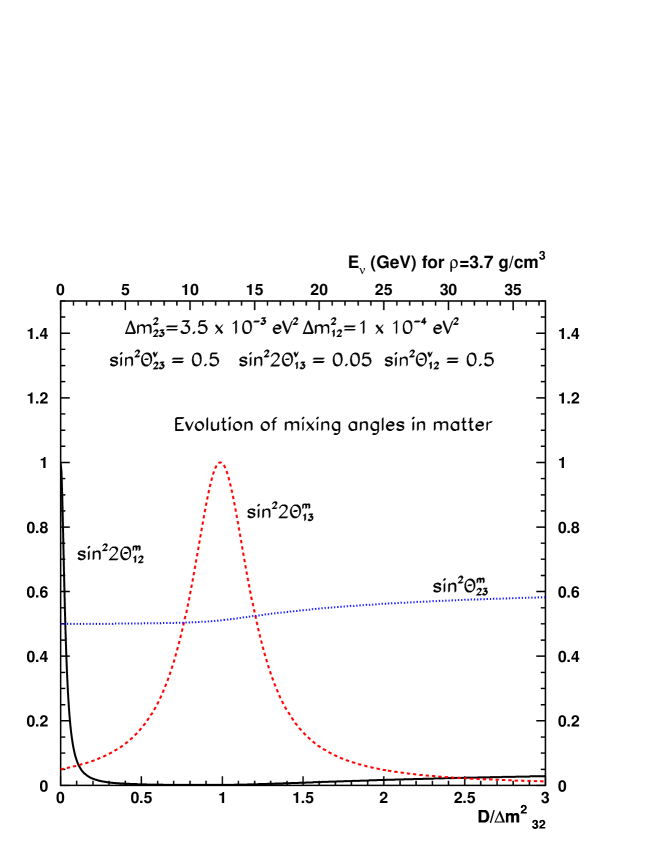
Figure 1: Evolution of mixing angles in matter as a function of $D(=2\sqrt{2}G_{F}N_{e}E_{\nu})/\Delta m^{2}_{32}$. The reference vacuum parameters are given in the figure.

Within the two-family mixing scheme, the modification of the flavor transition in matter is taken into account by the mixing angle in matter $\theta_{m}$, which is:

$$\sin^{2}2\theta_{m}(D)=\frac{\sin^{2}2\theta}{\sin^{2}2\theta+(\frac{D}{\Delta m^{2}}-\cos 2\theta)^{2}}$$ (12)

For neutrinos, a resonance condition will be met when $D\simeq\Delta m^{2}\cos 2\theta$ and the oscillation amplitude will reach a maximum. The resonant neutrino energy $E^{res}$ is

$$E^{res}\approx\frac{1.32\times 10^{4}\cos 2\theta\Delta m^{2}(eV^{2})}{\rho(g/cm^{3})}$$ (13)

Rather than two-family mixing, we have adopted throughout this study three-family framework. In this context, we use the analytic expressions for the matter mixing angles and mass eigenvalues calculated in [23, 24] (see Appendix A).

The mass eigenvalues in matter $M_{1}$, $M_{2}$ and $M_{3}$ are:

$$M_{1}^{2} = m_{1}^{2}+\frac{A}{3}-\frac{1}{3}\sqrt{A^{2}-3B}S-\frac{\sqrt{3}}{3}\sqrt{A^{2}-3B}\sqrt{1-S^{2}}$$ (14)

$$M_{2}^{2} = m_{1}^{2}+\frac{A}{3}-\frac{1}{3}\sqrt{A^{2}-3B}S+\frac{\sqrt{3}}{3}\sqrt{A^{2}-3B}\sqrt{1-S^{2}}$$ (15)

$$M_{3}^{2} = m_{1}^{2}+\frac{A}{3}+\frac{2}{3}\sqrt{A^{2}-3B}S$$ (16)

where $A$, $B$ and $S$ are given in the Appendix. For the mixing angles in matter the analytical expressions read:

$$\sin^{2}\theta^{m}_{12} = \frac{-(M_{2}^{4}-\alpha M_{2}^{2}+\beta)\Delta M^{2}_{31}}{\Delta M^{2}_{32}(M_{1}^{4}-\alpha M_{1}^{2}+\beta)-\Delta M^{2}_{31}(M^{4}_{2}-\alpha M_{2}^{2}+\beta)}$$ (17)

$$\sin^{2}\theta^{m}_{13} = \frac{M_{3}^{4}-\alpha M_{3}^{2}+\beta}{\Delta M^{2}_{31}\Delta M^{2}_{32}}$$ (18)

$$\sin^{2}\theta^{m}_{23} = \frac{G^{2}s^{2}_{23}+F^{2}c^{2}_{23}+2GFc_{23}s_{23}c_{\delta}}{G^{2}+F^{2}}$$ (19)

where $\alpha$, $\beta$, $G$ and $F$ are found in the Appendix.

To illustrate matter effects in three-neutrino mixing framework, we show in Figure 1 the values of the mixing angles in matter, plotted as a function of $D/\Delta m^{2}_{32}$, or equivalently of $\rho\times E$. The parameter values in vacuum correspond to our reference values for atmospheric and LMA-MSW solar experiments. The resonant behavior of $\theta^{m}_{13}$ is clearly visible. It gives maximum oscillation at a neutrino energy of about 12 GeV for a density of 3.7 $g\ cm^{-3}$. There is a similar resonant behavior for $\theta^{m}_{12}$ but it occurs at low energy since it is driven by $\Delta m^{2}_{21}$. For $D>\Delta m^{2}_{32}$, the angles $\sin^{2}2\theta^{m}_{12}$ and $\sin^{2}\theta^{m}_{23}$ tend to rise slightly, because the non-vanishing $\Delta m^{2}_{21}$ splitting removes the degeneracy between muon and tau flavors.

Our results have been computed assuming a constant density along the whole neutrino path, and equal to the mean density, obtained integrating over the earth profile [21]. This approximation yields, as shown in e.g. Ref. [25], similar results to those obtained by numerical integration using the actual Earth’s density profile.

The oscillation probability through matter will be a function of eight parameters: (a) the vacuum three mixing angles $\theta_{12}$,$\theta_{13}$,$\theta_{23}$; (b) the vacuum two mass differences squared $\Delta m^{2}_{12}$, $\Delta m^{2}_{23}$; (c) the average earth density $\rho$; (d) the baseline L; (e) the neutrino energy $E$.

3 Choice of baseline and event rates

The exact parameters of a neutrino factory are not yet completely fixed and realistic scenarios are in the process to be defined[10]. However, based on [10], we can assume that the muons in the storage ring have an energy $E_{\mu}=30$ GeV and that after one year of operation, the factory should deliver about $10^{20}$ “useful” muons decays of both polarities in the straight section pointing towards the far detector location. We base our ultimate reach on $10^{21}$ “useful” muons decays. Even an integrated intensity of $10^{22}$ might be eventually reachable.

We compute the fluxes assuming unpolarized muons and disregarding muon beams divergences within the storage ring. We integrate the expected event rates using a neutrino-nucleon Monte-Carlo generator [28]. The total charged current (CC) cross section is technically subdivided into three parts: the exclusive quasi-elastic scattering channel $\sigma_{QE}$ and the inelastic cross section $\sigma_{inelasic}$ which includes all other processes except charm production which is included separately.

Event rates for various baselines
		L=732 km		L=2900 km		L=7400 km
		$N_{tot}$	$N_{qe}$	$N_{tot}$	$N_{qe}$	$N_{tot}$	$N_{qe}$
	${\nu_{\mu}}$ CC	226000	9040	14400	576	2270	90
$\mu^{-}$	${\nu_{\mu}}$ NC	67300	$-$	4120	$-$	680	$-$
$10^{20}$ decays	$\bar{\nu}_{e}$ CC	87100	3480	5530	220	875	35
	$\bar{\nu}_{e}$ NC	30200	$-$	1990	$-$	300	$-$
	$\bar{\nu}_{\mu}$ CC	101000	4040	6380	255	1000	40
$\mu^{+}$	$\bar{\nu}_{\mu}$ NC	35300	$-$	2240	$-$	350	$-$
$10^{20}$ decays	${\nu_{e}}$ CC	197000	7880	12900	516	1980	80
	${\nu_{e}}$ NC	57900	$-$	3670	$-$	580	$-$

Table 1: Expected events rates for a 10 kton (fiducial) detector in case no oscillations occur for $10^{20}$ muon decays. $N_{tot}$ is the total number of events and $N_{qe}$ is the number of quasi-elastic events.

Table 1 summarizes the expected rates for the 10 kton fiducial mass and $10^{20}$ muon decays (expected 1 year of operation). $N_{tot}$ is the total number of events and $N_{qe}$ is the number of quasi-elastic events.

Even though our study is site non-specific, the chosen baselines could correspond to the distances between the Laboratori Nazionale del Gran Sasso (LNGS) and neutrino factories at (1) CERN ($L=732$ km, $<\rho_{Earth}>=2.8$ g/cm³), (2) Canary Islands ($L=2900$ km, $<\rho_{Earth}>=3.2$ g/cm³) and (3) Fermilab ($L=7400$ km, $<\rho_{Earth}>=3.7$ g/cm³).

4 The four main classes of events

Muon identification, charge and momentum measurement provide discrimination between $\nu_{\mu}$ and $\bar{\nu}_{\mu}$ charged current (CC) events. Good $\nu_{e}$ CC versus $\nu$ NC discrimination relies on the fine granularity of the target. Finally, the identification of $\nu_{\tau}$ CC events requires a precise measurement of all final state particles.

It is natural to classify the events in four classes[11]. We illustrate them for the case of $\mu^{-}$ stored in the ring.

1. Right sign muons ($rs\mu$): the leading muon has the same charge as those circulating inside the ring. Their origin is from

   1. non-oscillated ${\nu_{\mu}}$ CC

   2. ${\nu_{\mu}}\rightarrow{\nu_{\tau}}$ CC, $\tau^{-}\rightarrow\mu^{-}$ decays

   3. hadron decays in neutral currents.

2. Wrong sign muons ($ws\mu$): the leading muon has opposite charge to those circulating inside the ring. Opposite-sign leading muons can only be produced by neutrino oscillations, since there is no component in the beam that could account for them.

   1. $\bar{\nu}_{e}\rightarrow\bar{\nu}_{\mu}$ oscillations

   2. $\bar{\nu}_{e}\rightarrow\bar{\nu}_{\tau}$ oscillations, $\tau^{+}\rightarrow\mu^{+}$ decays

   3. hadron decays in neutral currents.

3. Electrons ($e$): events with a prompt electron and no primary muon identified. Events with leading electron or positron are produced by the charged-current interactions of the following neutrinos:

   1. non-oscillated $\bar{{\nu_{e}}}$ neutrinos

   2. ${\nu_{\mu}}\rightarrow{\nu_{e}}$ oscillations

   3. $\bar{\nu}_{e}\rightarrow\bar{\nu}_{\tau}$ or ${\nu_{\mu}}\rightarrow{\nu_{\tau}}$ oscillations with $\tau\rightarrow e$ decays

4. No Lepton ($0\ell$): events corresponding to NC interactions or $\nu_{\tau}$ CC events followed by a hadronic decay of the tau lepton. Events with no leading electrons or muons will be used to study the ${\nu_{\mu}}\rightarrow{\nu_{\tau}}$ oscillations. These events can be produced in

   1. neutral current processes

   2. $\bar{\nu}_{e}\rightarrow\bar{\nu}_{\tau}$ or ${\nu_{\mu}}\rightarrow{\nu_{\tau}}$ oscillations with $\tau\rightarrow hadrons$ decays

The last two classes can only be cleanly studied in a fine granularity detector.

The most effective way to fit the oscillation parameters is to study the visible energy distribution of the four classes of events defined above, since assuming the unoscillated spectra are known, they contain direct information on the oscillation probabilities.

Of course, for electron or muon charged current events, the visible energy reconstructs the incoming neutrino energy. In the case of neutral currents or the charged current of tau neutrinos, the visible energy is less than the visible energy because of undetected neutrinos in the final state. The information is in this case degraded but can still be used.

Our analyses are performed on samples of fully generated Monte-Carlo[28] events, which include proper kinematics of the events, full hadronization of the recoiling jet and proper exclusive polarized tau decays when relevant. Nuclear effects, which are taken into account by the FLUKA model [29], are included as they are important for a proper estimation of the tau kinematical identification.

The detector response is included in our analyses using a fast simulation which parameterizes the momentum and angular resolution of the emerging particles, using essentially the following values: electromagnetic shower $3\%/\sqrt{E}\oplus 1\%$, hadronic shower $\approx 20\%/\sqrt{E}\oplus 5\%$, and magnetic muon momentum measurement $20\%$.

Hadron decay background can be quite large in a low density target and could be quite dangerous. Fortunately, it can be easily suppressed by a cut on the muon candidate momentum, $P_{\mu}>2$ GeV, which reduces it to a tolerable level. Figure 2 illustrates the relative background expected for $\nu_{\mu}$ and $\bar{\nu}_{\mu}$ NC and CC processes as a function of the muon momentum. After the cut, the expected contamination for $\nu_{\mu}$ CC events is at the level of $10^{-5}$. Real charged current events maintain an efficiency above $95\%$.

Figure 2: Fractional background due to the decay of charged mesons as a function of the measured muon momentum.

The visible energy is computed as the modulus of the vector sum of the momenta of each visible particle in the event. Figures 6, 6, 6 and 6 show the reconstructed visible energy at the baseline $L=7400$km normalized to $10^{20}\mu$’s for each event class for a specific oscillation scenario with $\Delta m_{32}^{2}=3.5\times 10^{-3}$ eV², $\sin^{2}\theta_{23}=0.5$ and $\sin^{2}2\theta_{13}=0.05$. The different contributions including backgrounds for each event class have been evidenced in the plots. For example, in Figure 6, the different processes that contribute to the right-sign muon class are unoscillated muons, taus and background events.

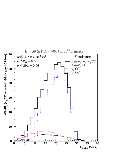
Figure 3: Visible energy spectrum for electron events: $\nu_{e}$ CC (dashed line), $\nu_{\tau}$ and $\bar{\nu}_{\tau}$ (dotted line) and $\bar{\nu}_{e}$ CC (dot-dashed). The solid histogram shows the sum of all contributions.

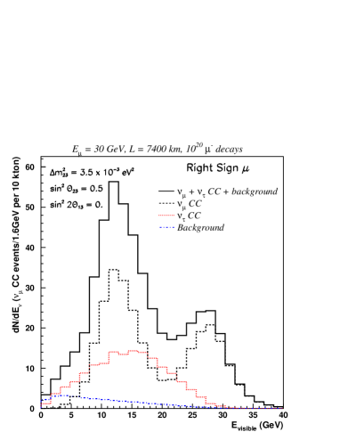
Figure 4: same as Figure 6 for right-sign muon sample: $\nu_{\mu}$ CC (dashed line), $\nu_{\tau}$ and $\bar{\nu}_{\tau}$ (dotted line) and meson decay background (dot-dashed). The solid histogram shows the sum of all contributions.

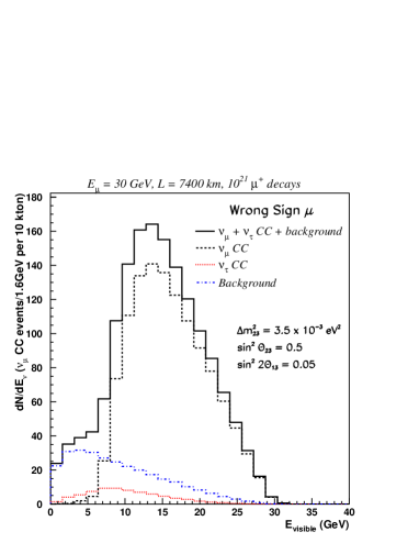
Figure 5: same as Figure 6 for wrong sign muon sample: $\nu_{\mu}$ CC (dashed line), $\nu_{\tau}$ and $\bar{\nu}_{\tau}$ (dotted line) and meson decay background (dot-dashed). The solid histogram shows the sum of all contributions.

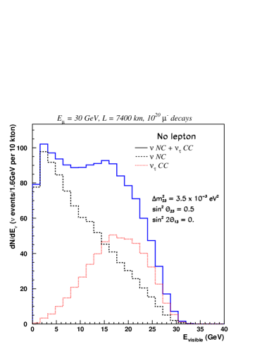
Figure 6: same as Figure 6 for the no-lepton sample: $\nu$ NC (dashed line), $\nu_{\tau}$ and $\bar{\nu}_{\tau}$ (dotted line). The solid histogram shows the sum of all contributions.

5 Further classification based on kinematical analysis

$\nu_{\mu}\rightarrow\nu_{\tau}$ appearance search
Cuts	$\tau\rightarrow l$	CC background	Cuts	$\tau\rightarrow h$	NC background
Initial	$100\%$	$100\%$	Initial	$100\%$	$100\%$
Loose cuts
$P_{T}^{l}<0.5$GeV	$50\%$	$14\%$	$P_{T}^{miss}<1$GeV	$72\%$	$40\%$
$P_{T}^{miss}>0.6$GeV	$40\%$	$0.5\%$	$Q_{T}>0.5$GeV	$30\%$	$2\%$
Tight cuts
$P_{T}^{l}<0.5$GeV	$50\%$	$14\%$	$P_{T}^{miss}<1$GeV	$72\%$	$40\%$
$P_{T}^{miss}>1$GeV	$20\%$	$0.08\%$	$Q_{T}>1$GeV	$6\%$	$0.07\%$

Table 2: $\nu_{\tau}$ appearance search for the leptonic and hadronic decay modes of the tau lepton. Overall signal efficiencies and fractional remaining backgrounds are quoted. The case labelled as “Tight cuts” correspond to the situation where one event background is expected, for $10^{20}$ muon decays, at the farthest location ($L=7400$ km).

An efficient identification of $\nu_{\tau}$ induced charged current events requires a precise measurement of all final state particles. Excellent calorimetry allows to take full advantage of the special kinematic features of $\nu_{\tau}$ events. We independently search for the leptonic and hadronic tau decay modes.

For the $\tau\rightarrow l\nu\nu$ decay mode, the main background comes from $\nu_{l}$ CC. To enhance the separation between $\tau$ and background events, we demand the event missing $P_{T}$ to be larger than 0.6 GeV and the transverse momentum of the lepton candidate,$P_{T}^{l}$, to be smaller than 0.5 GeV. This set of cuts is referred to as “loose cuts” and it will be used to perform a check on appearance/disappearance consistency (see subsection 9). In Table 2, we show that the overall $\tau$ efficiency for “loose cuts” is $40\%$ for a CC background level of $\sim 5\times 10^{-3}$. Figure 7 shows the energy spectra for the four event classes after application of these cuts, for $\nu_{\tau}$ CC and other types of events. No energy cut has been applied, but the fact of using the energy spectra in the fit also exploits the difference in energy spectra of $\nu_{\tau}$ CC events.

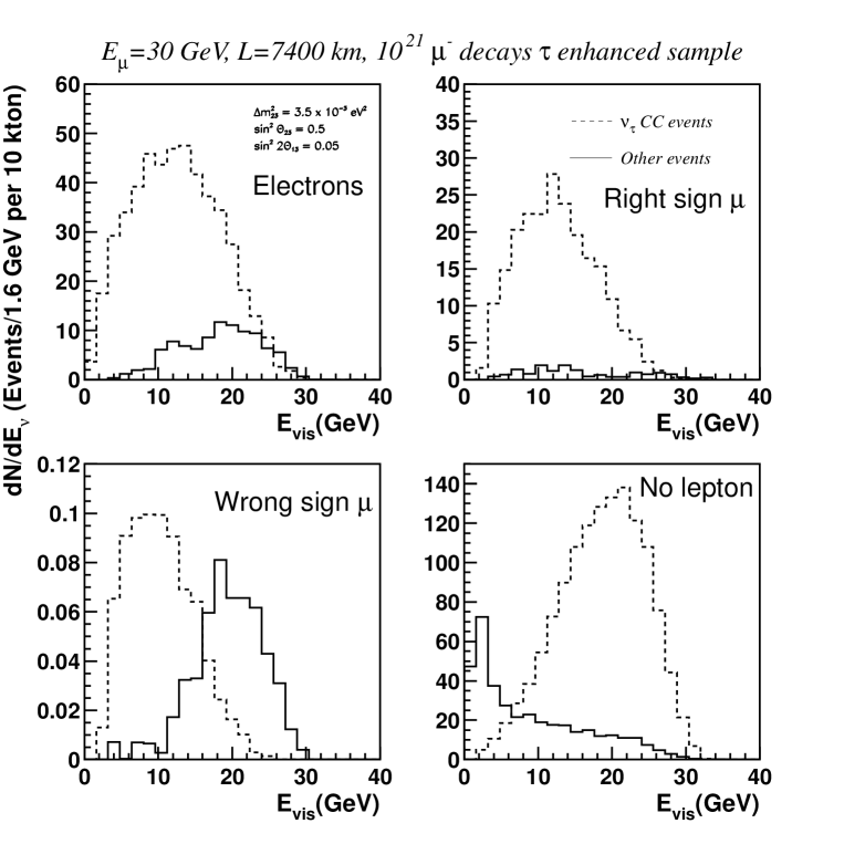
Figure 7: Visible energy spectrum for the four event classes after application of loose kinematic cuts (see text). The presence of $\tau$ events in the third class (wrong-sign muons) is an indication of the process $\nu_{e}\rightarrow\nu_{\tau}$.

A set of “tight cuts” is also applied, aiming at having one expected background event at the farthest location in case $10^{20}$ “useful” muons decays are delivered. As we can see from Table 2, the overall tau efficiency in this case amounts up to $20\%$.

For hadronic decays the most important source of background correspond to NC events. If we demand a $P_{T}^{miss}$ smaller than 1 GeV and a transverse momentum of the hadron candidate with respect to the total event momentum, $Q_{T}$, larger than 0.5 GeV (“loose cuts”) only $2\%$ of the initial background survives for an overall tau efficiency of $30\%$. If we require only one NC background event survivor at $L=7400$ km (“tight cuts”), the signal efficiency drops to $6\%$ due to the stringent $Q_{T}$ requirement imposed.

6 Quasi-elastic final states

The quasi-elastic process, while rare, is a clean process that allows to separate neutrino from anti-neutrino events, in principle for all neutrino flavors, since $\nu_{\ell}+n\rightarrow\ell^{-}+p$ and $\bar{\nu}_{\ell}+p\rightarrow\ell^{+}+n$. The recoil proton is easily identifiable within the high-granularity target.

This channel is particularly interesting to study oscillation in the electron channel. Starting from negative muons circulating in the storage ring, we look for exclusive electron-proton final states. These provide “background-free” oscillation signals:

$$\mu^{-}\rightarrow e^{-} \bar{\nu_{e}} {\nu_{\mu}}$$ (21)

$$\rightarrow{\nu_{e}}+n\rightarrow e^{-}+p$$

$$\rightarrow{\nu_{\tau}}+n\rightarrow\tau^{-}+p\rightarrow e^{-}\nu\nu+p$$

since $\bar{\nu_{e}}+p\rightarrow e^{+}+n$.

The selection of quasi-elastic events is the only way to identify the helicity of neutrino electrons in absence of measurement of the electron charge.

7 Oscillation parameters fitting

Given the adopted parameterization of the mixing matrix, we have a priori a total of 7 free parameters, which can be represented by the vector:

$$\vec{P}=(\Delta m^{2}_{21},\Delta m^{2}_{32},\sin^{2}\theta_{12},\sin^{2}2\theta_{13},\sin^{2}\theta_{23},\delta,\rho)$$ (22)

The values of the parameters governing the oscillations are extracted from a global fit of the visible energy distributions obtained for each event class. The fit is performed with the MINUIT [22] package, and is expected to get back the same values of the parameters, starting from the reference distributions.

At each iteration, a different set of parameters is probed, and with the same procedure used to get the reference histograms.

For a given polarity $\lambda$ of the muons in the storage ring, we compute $\chi^{2}$’s of the difference between the binned oscillated spectra, which will be function of the parameters, and the reference histograms. We define a $\chi^{2}$ for each of the four classes of events, i.e. the electrons ($e$), the right-sign muon ($rs\mu$), the wrong sign muons ($ws\mu$) and the no lepton class ($0\ell$):

$$\chi^{2}_{\lambda,all}=\chi^{2}_{\lambda,e}+\chi^{2}_{\lambda,rs\mu}+\chi^{2}_{\lambda,ws\mu}+\chi^{2}_{\lambda,0\ell}$$ (23)

where

$$\chi^{2}_{\lambda,c}(\vec{P})=\sum_{i}\left(\frac{N^{c}_{i}(\vec{P})-N_{i}^{c}(\vec{P}_{ref})}{\sigma^{2}_{i,c}}\right)^{2}.$$ (24)

The sum runs over 25 equally spaced energy bins ($E_{i}$, $i=1,25$). Here, $N^{c}_{i}(\vec{P}_{ref})$ is the expectation for the reference values and $N^{c}_{i}(\vec{P})$ is the “data” obtained for a given set of the oscillation parameters $\vec{P}$. $\sigma_{i,c}$ contains both statistical and systematic contributions to the total error. In order to improve the statistical treatment of bins with low statistics, a bin that possesses less than 40 events is assumed to be Poisson distributed and therefore its contribution is computed as $2(N^{c}_{i}(\vec{P})-N^{c}_{i}(\vec{P}_{ref}))+2N_{i}\ln(N^{c}_{i}(\vec{P})/N^{c}_{i}(\vec{P}_{ref}))$ (see Ref. [30]).

The systematic error takes into account the uncertainties in the knowledge of the beam, neutrino cross sections and selection efficiencies and we assume it amounts up to $2\%$ uncorrelated from bin to bin.

We assume that a neutrino factory will operate with alternate runs of opposite muon polarities, therefore eight energy distributions can be fitted simultaneously:

$$\chi^{2}_{all}=\chi^{2}_{+,all}+\chi^{2}_{-,all}$$ (25)

The values of the fitted parameters $\vec{P}$ are obtained minimizing the $\chi^{2}(\vec{P})$.

It is in practice not always possible to fit all the free parameters, since for some parameter-space regions, the oscillation effects at the chosen baselines and energies can be negligible. In particular, this can be the case for $\Delta m^{2}_{21}$ and $\sin^{2}\theta_{12}$ which drive the solar oscillations. For values $\Delta m^{2}_{21}\ll 10^{-4}\ \rm eV^{2}$, we are insensitive to the “solar” sector.

We therefore adopted successive fitting procedures with an increasing number of free parameters.

At first, we can simplify the three-family oscillation picture if the oscillations produced by $\Delta m^{2}_{21}$ can be neglected at the considered baselines and energies. In this case, only the mass difference squared $\Delta m^{2}_{32}$ and the two mixing angles $\theta_{13}$ and $\theta_{23}$ are relevant. The oscillation probabilities are given in the Appendix. For example, for ${\nu_{e}}\rightarrow{\nu_{\mu}}$ oscillations, it is:

$$P({\nu_{e}}\rightarrow{\nu_{\mu}},E,L)=\sin^{2}(2\theta^{m}_{13})\sin^{2}(\theta^{m}_{23})\Delta^{2}_{32}$$ (26)

where $\Delta^{2}_{32}=\sin^{2}\left((M_{3}^{2}-M_{2}^{2})L/4E\right)$. The fit has in this case 4 free parameters, which can be represented by the vector:

$$\vec{P}_{1ms}=(\Delta m^{2}_{32},\sin^{2}2\theta_{13},\sin^{2}\theta_{23},\rho)$$ (27)

The $\delta$ phase has disappeared, since within this approximation it becomes unphysical. The results are presented in Section 8, assuming a $\Delta m^{2}_{32}$ parameter varying in the range of values favoured by current atmospheric data ($\Delta m^{2}_{32}=3.5,5,7\times 10^{-3}\ {\rm eV}^{2}$), a maximal (2-3)-mixing $\sin^{2}\theta_{23}=0.5$ and a $\theta_{13}$ value compatible with CHOOZ results [26] and recent fits to data [27] ($\sin^{2}2\theta_{13}=0.05$).

We return to the general three-family scenario in Section 10 where we consider sensitivity to the $CP$ violation.

In order to compute the precision of the determination of the parameters, we consider two methods: (1) a one-dimensional “scan” of a given parameter; the other variables are left free and mininized at each step; the resp. 1,2,3 sigmas are given by resp. $\chi^{2}_{min}+1$, $+4$ and $+9$. (2) a two-dimensional “scan” of a two-parameter plane; the other variables are left free and minimized at each point in the plane; the resp. 68%, 90%, 99% C.L. are given by resp. $\chi^{2}_{min}+2.3$, $+6.0$ and $+9.2$.

8 Results for one mass scale approximation

8.1 Case of two-family mixing : $\theta_{13}=0$

Two family mixing
$\delta(\sin^{2}\theta_{23})$ for $\theta_{23}=45^{o}$, $\theta_{13}=0$
	Only right-sign muons		All classes
	$\chi^{2}_{\pm,rs\mu}$		$\chi^{2}_{\pm,all}$
$\Delta m^{2}_{32}$ (eV2)	L=7400 km	L=2900 km	L=7400 km	L=2900 km
$7\times 10^{-3}$	$22\%$	$8\%$	$20\%$	$8\%$
$5\times 10^{-3}$	$12\%$	$12\%$	$11\%$	$10\%$
$3.5\times 10^{-3}$	$10\%$	$18\%$	$10\%$	$16\%$

Table 3: Precision in the measurement of the mixing angle assuming two family mixing for three possible mass differences and two very large baselines.In all the cases the precision obtained in the measurement of $\Delta m_{32}^{2}$ is $1\%$.

The detection of the dip in the energy distribution of the right-sign muon sample dominates the precision on the measurement of the mixing angle $\theta_{23}$ and the mass difference $\Delta m^{2}_{32}$. This is true provided that the beam energy and baseline are chosen in such a way that the ${\nu_{\mu}}$ disappearance maximum is visible in the oscillated spectrum. Table 3 summarizes the expected accuracies. With $10^{20}$ muon decays of each polarity, precisions of $1-2\%$ are expected in the determination of $\Delta m^{2}_{32}$ while for the precision on $\sin^{2}\theta_{23}$ is around 10$\%$, in agreement with results quoted in [14].

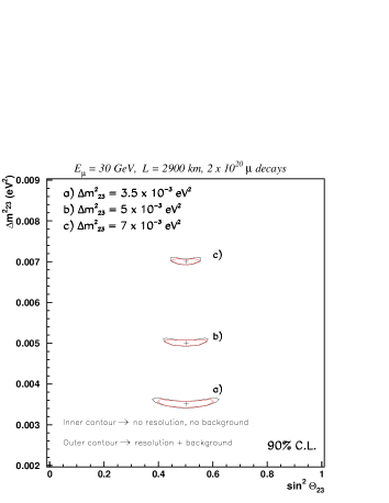
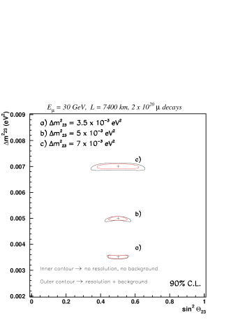
Figure 8: Two-dimensional 90%C.L. contours for $\Delta m^{2}_{32}$ and $\sin^{2}\theta_{23}$ for three different $\Delta m^{2}_{32}$ values. Inner contours: no background and perfect muon resolution; outer contours: backgrounds and muon resolution included.

We compare in figure 8 how the precision on the mass difference and mixing angle changes when experimental resolutions and backgrounds are disregarded. We see that our fits are barely affected and only for the cases where the dip is not seen, the instrumental effects and backgrounds spoil at the level of a few per cent the accuracy on the oscillation parameters.

8.2 Case of three-family mixing : $\theta_{13}\neq 0$

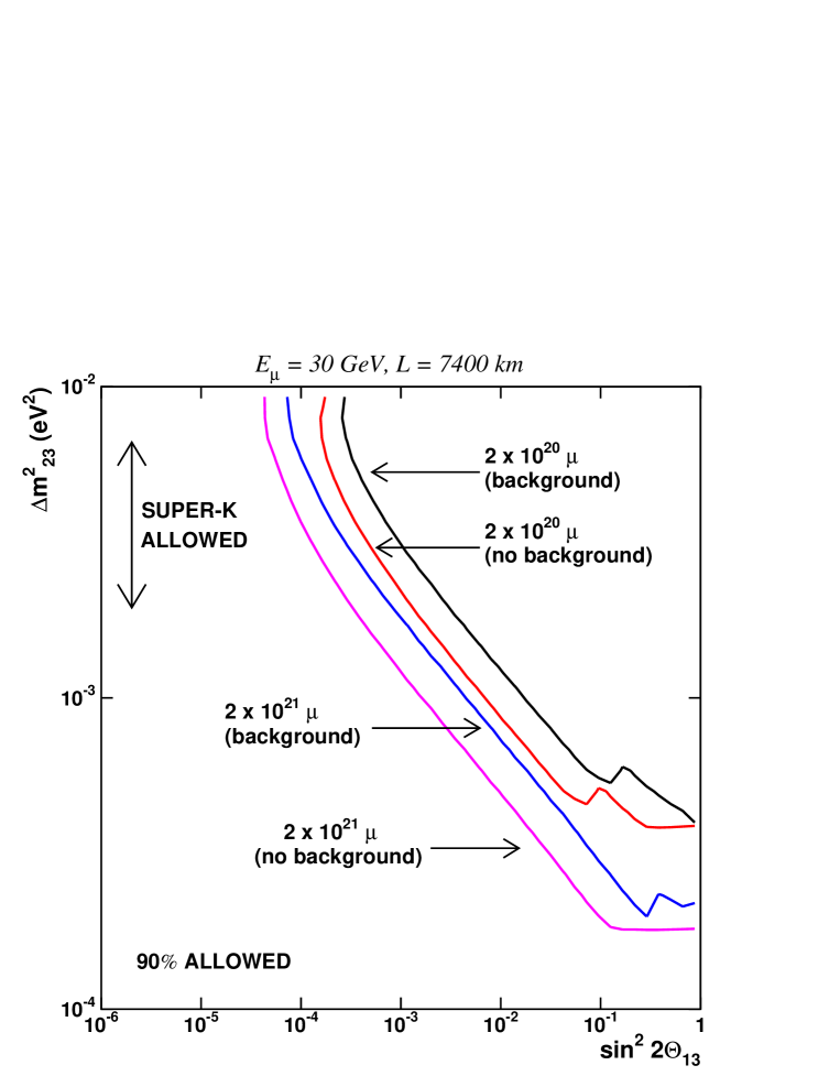
Figure 9: Sensitivity on $\theta_{13}$

In order to obtain the best sensitivity on the mixing angle $\theta_{13}$, the search for wrong sign muons is ideal, since it will be a direct signature for ${\nu_{e}}\rightarrow{\nu_{\mu}}$ oscillations.

For this kind of study, since we are dealing with the smallest number of signal events, the sensitivity does strongly depend on the ability of rejecting background. Figure 9 shows for $L=7400$ km, the sensitivity on $\theta_{13}$ for two different muon normalizations ($10^{20}$and $10^{21}$ muon decays of each polarity). For each pair of values $(\Delta m^{2}_{32},\ \theta_{13})$, the fit was performed leaving $\theta_{23}$ free.

In the obtaining previous plot, we did not on purpose apply strong background cuts, since we believe that very high rejection powers obtained on paper may not stand the proof of real experimental conditions, with non-gaussian behaviours, tails of distributions etc.

To also give the maximum of sensitivity that can be obtained in principle, we also illustrated in figure 9 the effect that a background free environment would have in the expected sensitivity. At 90$\%$ C.L., we obtain $\sin^{2}2\theta_{13}<10^{-3}-10^{-4}$ depending on the number of muon decays. This represents two orders of magnitude improvement with respect to quoted sensitivities at CNGS. In case we consider $10^{21}$ muon decays and backgrounds are reduced to a negligible level, the obtained sensitivity is consistent with the one quoted in [18].

For a background-free environment gives the best sensitivity, the amount of information added by other event classes (i.e. the electrons) is negligible.

8.2.1 Determination of $\theta_{13}$

The measurement of $\theta_{13}$ can profit from long baselines, since matter effects will enhance the oscillation signal. In presence of backgrounds, it is more favorable to enhance neutrinos signal even at the cost of the suppression of the anti-neutrino oscillations.

Table 4 summarizes the expected precision on the measurement of the oscillation parameters.

In this case, since for the chosen value of $sin^{2}2\theta_{13}=0.05$ the number of signal events is quite large, there is not any more a strong need for a background-free environment. Therefore, the inclusion of other event classes, like the electrons, can help to constrain the oscillation parameters.

Three-family mixing
$\sin^{2}\theta_{23}=0.5$, $\sin^{2}2\theta_{13}=0.05$
	All classes		Only muons
	$\chi^{2}_{all}$		$\chi^{2}_{rs\mu}+\chi^{2}_{ws\mu}$
	L=2900 km	L=7400 km	L=2900 km	L=7400 km
$\Delta m^{2}_{32}=3.5\times 10^{-3}$ eV2,
$\delta(\Delta m^{2}_{32})$	$1.4\%$	$0.9\%$	1.4%	0.9%
$\delta(\sin^{2}\theta_{23})$	$14\%$	$8\%$	16%	9%
$\delta(\sin^{2}2\theta_{13})$	$15\%$	$10\%$	17%	15%
$\Delta m^{2}_{32}=5\times 10^{-3}$ eV2
$\delta(\Delta m^{2}_{32})$	$0.4\%$	$0.8\%$	0.4%	0.8%
$\delta(\sin^{2}\theta_{23})$	$11\%$	$8\%$	10%	12%
$\delta(\sin^{2}2\theta_{13})$	$11\%$	$9\%$	14%	16%
$\Delta m^{2}_{32}=7\times 10^{-3}$ eV2
$\delta(\Delta m^{2}_{32})$	$0.4\%$	$0.6\%$	0.4%	0.6%
$\delta(\sin^{2}\theta_{23})$	$7\%$	$8\%$	8%	18%
$\delta(\sin^{2}2\theta_{13})$	$8\%$	$6\%$	9%	20%

Table 4: Precision on the measurement of the oscillation parameters.

8.3 Sensitivity to $\theta_{13}$ with quasi-elastic events

${\nu_{e}}$ appearance search with quasi-elastic
Electron Class: Events for $10^{21}\ \mu^{-}$ decays
	$\bar{\nu}_{e}$ CC		$\nu_{\mu}\rightarrow\nu_{e}$ CC		$\nu_{\mu}\rightarrow\nu_{\tau}$ CC, $\tau\rightarrow e$
Baseline	Total	Elastic	Total	Elastic	Total	Elastic
$L=732$ km	860000	43000	2090	84	3990	110
$L=2900$ km	54300	2700	1720	70	3300	90
$L=7400$ km	8300	410	960	40	1450	40

Table 5: Expected number of electron type events for $10^{21}\ \mu^{-}$ decays. The three contributions to the total number of electron events are shown separately. Rates have been computed assuming oscillations with $\Delta m^{2}_{32}=3.5\times 10^{-3}$ eV², $\sin^{2}\theta_{23}=0.5$ and $\sin^{2}2\theta_{13}=0.05$.

An exclusive way of detecting the effects of a non vanishing $\theta_{13}$ is through the appearance of wrong sign electrons. Although, with the assumed detector configuration, there is no ability to directly measure the charge of the leading electrons, there is the possibility of disentangling final state electrons from positrons through the use of quasi-elastic events. We look for electron-proton final states. For example, in the target of ICANOE, a proton can be resolved if its kinetic energy is larger than about 100 MeV corresponding to a range of more than 2 cm.

Table 5 shows the expected rates contributing to the electron class before any cut is applied. The background is twofold: (a) quasi-elastic $\nu_{\tau}$ CC events followed by $\tau\rightarrow e$, (b) $\bar{\nu}_{e}$ CC with an extra proton from nuclear origin.

This last background can be estimated from data themselves studying the reaction $\bar{\nu}_{\mu}p\rightarrow\mu^{+}n$. Demanding a back to back electron-proton event topology with a proton kinetic energy in excess of 100 MeV, we estimate the expected background to be less than one event for an overall signal efficiency of $50\%$.

The quasi-elastic channel provides, in a “background free” environment, 20 to 40 gold-plated events depending on the selected baseline. It is very clean channel but is limited by statistics.

8.4 Fit of the average Earth density parameter

In matter, the amplitude of neutrino oscillation goes through a maximum for an energy given by equation 13. Since $\theta_{13}$ is small, the MSW resonance peak is only a function of $\rho$ and $\Delta m^{2}_{32}$, This can be seen in Figure 11. Since the mass difference is constrained by the disappearance of right-sign muons, $\rho$ is well-determined by the energy distribution of wrong sign muons.

We extract the density from the fit, leaving it as a free parameter, as well as $\Delta m^{2}_{32}$, $\theta_{23}$ and $\theta_{13}$. The precision on the determination of $\rho$ depends on the baseline, as shown in table 6, obtained considering $2\times 10^{21}$ muon decays. For the longest baseline, where matter effect are large, a precision as good as 2% can be obtained.

Distance (km)	Density (g/cm3)	Relative error (%)
732	2.8	18
2900	3.2	10
7400	3.7	2

Table 6: Precision on the determination of $\rho$, from a global fit where also $\Delta m^{2}_{32}$, $\theta_{23}$ and $\theta_{13}$ are left as free parameters. This result has been obtained for $2\times 10^{21}$ muon decays.

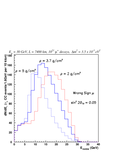
Figure 10: Variation of the MSW resonance peak for wrong sign muons as a function of Earth’s density. The plot is normalized to $10^{21}\ \mu^{+}$ decays.

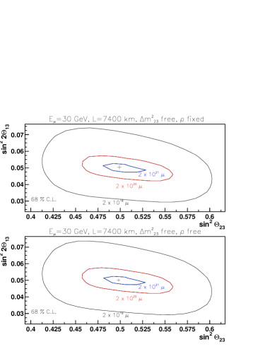
Figure 11: 68%C.L. two-dimensional contours for $\sin^{2}2\theta_{13}$ and $\sin^{2}\theta_{23}$: influence of $\rho$ in the determination of the mixing angles for three different muon normalizations and $L=7400$ km. In the upper plot $\rho$ is fixed during the fit, while in the lower one is taken as a free parameter.

The influence of $\rho$ in our fits is addressed in figure 11. We see that for $L=7400$ km and three different muon normalizations, the fact that $\rho$ is either considered as a free parameter or fixed during the fit does not influence the accuracy in the determination of the mixing angles.

9 Over-constraining the oscillation parameters

The information about the oscillation parameter is redundantly available in the visible energy distributions of the various event classes. This allows us to address the question of the consistency between the different observed oscillations processes.

Given the high statistical accuracy of the measurement, the consistency can be tested with good accuracy. In the three active neutrino mixing scheme, this implies that $\Sigma_{y=e,\mu,\tau}P(\nu_{x}\rightarrow\nu_{y})$ should be equal to one for $x=e,\mu,\tau$ and the same holds for anti-neutrinos.

Other models can predict different values (i.e., oscillations to sterile neutrinos exist, the sum would be smaller than one).

Let us concentrate on the oscillations into $\tau$ neutrinos. In the case of negative muons in the ring, they can be originated from $\nu_{\mu}\rightarrow\nu_{\tau}$ or $\bar{\nu}_{e}\rightarrow\bar{\nu}\tau$ oscillations. The latter case is particularly interesting, since coupling a neutrino factory with a detector with $\tau$ identification capabilities is probably the only way to identify and measure such a process. The $\bar{\nu}_{e}\rightarrow\bar{\nu}\tau$ can be revealed experimentally from the presence of $\tau$ candidates in the wrong-sign muon sample, due to the opposite helicity of electron and muon neutrinos in the beam.

To have a quantitative estimation of the consistency check of the various oscillation modes to $\tau$ neutrino, we assign two global normalization factors, $\alpha$ and $\beta$ to the oscillation probabilities $P(\nu_{\mu}\rightarrow\nu_{\tau})$ and $P(\nu_{e}\rightarrow\nu_{\tau})$. If no new phenomena occur, these parameters should be exactly one. From a global fit to the visible energy distributions it is possible to extract the values of these parameters, and the precision obtainable on their measurement.

Appearance/disappearance test
Baseline	$\Delta m^{2}_{32}$ ($\times 10^{-3}$ eV2)	$10^{20}\mu^{\pm}$	$10^{21}\mu^{\pm}$	$10^{22}\mu^{\pm}$
Precision on $\alpha\Rightarrow\alpha\times P(\nu_{\mu}\rightarrow\nu_{\tau})$
	3.5	$5.5\%$	$2\%$	$0.6\%$
7400 km	5	$6\%$	$2\%$	$0.6\%$
	7	$11\%$	$3\%$	$1\%$
	3.5	$4\%$	$2\%$	$0.6\%$
2900 km	5	$3\%$	$1\%$	$0.4\%$
	7	$2.5\%$	$1\%$	$0.4\%$
Precision on $\beta\Rightarrow\beta\times P(\nu_{e}\rightarrow\nu_{\tau})$
	3.5	$60\%$	$20\%$	$7\%$
7400 km	5	$35\%$	$10\%$	$5\%$
	7	$25\%$	$7\%$	$2\%$
	3.5	$75\%$	$25\%$	$9\%$
2900 km	5	$25\%$	$15\%$	$5\%$
	7	$30\%$	$10\%$	$4\%$

Table 7: Precision on the determination of the parameters $\alpha$ and $\beta$ that quantify, respectively, the amount of $\nu_{\mu}\rightarrow\nu_{\tau}$ and $\nu_{e}\rightarrow\nu_{\tau}$ present in the data. In the three neutrino framework, the reference values are $\alpha,\ \beta=1$.

To select $\tau$ events from the background, still retaining a high efficiency on the signal, we apply a set of loose kinematic cuts (see table 2).

Background levels of the order of one event can be reached applying tighter cuts, but in these cases the statistics is too small and the results obtained are slightly worse.

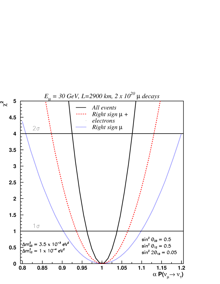
Figure 12: Precision on the determination of the $\alpha$ parameter when the fit is performed using: all event classes(solid line), right-sign muons + electrons(dashed line) and right-sign muons only(dotted line).

Since the $\tau$ lepton decays into muons, electrons and hadrons, we expect that a fit to all event classes would result in a remarkable improvement on the precision for the $\alpha$ parameter. Figure 12 shows how $\alpha$ determination improves as the different event classes are included in the fit.

Table 7 shows the expected precisions in the determination of $\alpha$ and $\beta$. We observe that for $10^{20}$ decays, $\alpha$ is better determined (accuracy around $5\%$) for $L=2900$km, however for $10^{21}$ muons, the accuracy is about $1\%$ regardless of the baseline and the mass difference and therefore $\nu_{\mu}$ oscillations into a sterile neutrino can be largely ruled out.

The accuracy on $\beta$, and therefore the first experimental evidence for $\nu_{e}\rightarrow\nu_{\tau}$ is much worst, given the smaller statistics available, since this oscillation probability is smaller than the corresponding $\nu_{\mu}\rightarrow\nu_{\tau}$ by a factor $\sin^{2}2\theta_{13}$, taken to be in this case 0.05. We observe that somewhat better determination exists at $L=7400$km since this oscillation mode is largely influenced by matter effects given its dependence on $\theta_{13}$. We conclude that a precision at the level of a few per cent on the observation of $\nu_{e}\rightarrow\nu_{\tau}$ oscillations would require $O(10^{22})$ useful muon decays.

10 Results for the general three-family scenario and CP-violation

Let us consider now a more complex scenario. In this case, the value of the mass difference $\Delta m^{2}_{12}$ is not any more negligible, and is actually assumed to be $10^{-4}eV^{2}$, one of the highest values compatible with the large mixing angle MSW solution for solar neutrinos [21].

The oscillation does not depend any more on only three parameters, but all four independent angles of the mixing matrix and the two mass differences become important.

In the most general case, the phase $\delta$ can be different from zero, producing a complex mixing matrix, and thus generating CP violation.

We recall that for neutrinos propagating in vacuum, the oscillation probability after a distance $L$ for neutrinos can be expressed as:

$$P(\nu_{\alpha}\rightarrow\nu_{\beta};E,L) = P_{CP\ even}(\alpha,\beta;E,L)+P_{CP\ odd}(\alpha,\beta;E,L)$$ (28)

and for antineutrinos :

$$P(\bar{\nu}_{\alpha}\rightarrow\bar{\nu}_{\beta};E,L) = P_{CP\ even}(\alpha,\beta;E,L)-P_{CP\ odd}(\alpha,\beta;E,L)$$ (29)

As an illustration, the probability for $\nu_{\mu}$ to $\nu_{e}$ conversion in vacuum, assuming three family mixing and CP-violation, is given by:

$$P_{CP\ odd}(\mu,e) = 2{\cos(\theta^{m}_{13})}^{2}\sin\delta^{m}\sin(2\theta^{m}_{12})\sin(\theta^{m}_{13})\sin(2\theta^{m}_{23})\times$$

$$\sin(\frac{\Delta M_{12}^{2}L}{4E})\sin(\frac{\Delta M_{13}^{2}L}{4E})\sin(\frac{\Delta M_{23}^{2}L}{4E})$$

where the $CP$-phase in matter is:

$$e^{-i\delta_{m}}=\frac{(G^{2}e^{-i\delta}-F^{2}e^{i\delta})s_{23}c_{23}+GF(c^{2}_{23}-s^{2}_{23})}{\sqrt{(G^{2}s^{2}_{23}+F^{2}c^{2}_{23}+2GFc_{23}s_{23}c_{\delta})(G^{2}c^{2}_{23}+F^{2}s^{2}_{23}-2GFc_{23}s_{23}c_{\delta})}}$$ (31)

Here, $G$ and $F$ are given in the Appendix.

In case of degenerate mass differences, $|\Delta m^{2}_{21}|\approx|\Delta m^{2}_{32}|$, the $\delta$ phase is significantly modified from its original value in vacuum for $\delta>\pi/4$ radians, while in the case $|\Delta m^{2}_{32}|>|\Delta m^{2}_{21}|$ the CP phase is almost unaffected by the presence of matter.

In addition, neutrino propagation in a dense medium makes more difficult to experimentally extract a genuine CP violation signal, since the asymmetrical behavior of matter, with respect to neutrinos and anti-neutrinos, induces fake CP violation effects.

10.1 $CP$ statistical significance

To evaluate the sensitivity to this kind of measurement as a function of the oscillation parameters and of the selected baseline, we compare the case where CP violation is maximal ($\delta=\pi/2$) and the case of no CP violation ($\delta=0$). Figure 13 shows the sensitivity

$$S_{CP}(E_{i})\equiv\frac{N(\delta=\pi/2,E_{i})-N(\delta=0,E_{i})}{\sqrt{N(\delta=0,E_{i})}}$$ (32)

i.e. the difference between the two extreme cases, divided by the statistical error (being N the number of events in each energy bin, for a given value of $\delta$). We can see that for the baseline of 732 km, this quantity is positive for almost the full energy range, so there is no real shape variation in the spectrum, and the CP effect is similar to what would be obtained with a change in the angle $\theta_{13}$. On the other hand, for larger baselines this curve crosses the zero, and the CP violation produces a visible deformation of the energy spectrum.

Figure 13: Statistical significance of CP violation effects for three possible $\Delta m^{2}_{32}$ values mass at the three considered baselines. $N(\delta=\pi/2)$ is the number of expected events assuming maximal CP violation in vacuum and $N(\delta=0)$ corresponds to the number of expected events in absence of CP violation, for $2\times 10^{21}$ muons

10.2 Fitting of the $\delta$ parameter

To evaluate the precision reachable on the measurement of these three oscillations parameters, we perform fits assuming the following reference values:

$$\Delta m^{2}_{32} = 3.5,5,7\times 10^{-3}\ {\rm eV}^{2}$$

$$\Delta m^{2}_{12} = 1\times 10^{-4}\ {\rm eV}^{2}$$

$$\sin^{2}\theta_{23} = 0.5\hskip 91.04872pt\theta_{23}=45^{o}$$

$$\sin^{2}2\theta_{13} = 0.05\hskip 82.51282pt\theta_{13}=6.5^{o}$$

$$\sin^{2}\theta_{12} = 0.5$$

$$\delta\geq 0$$ (33)

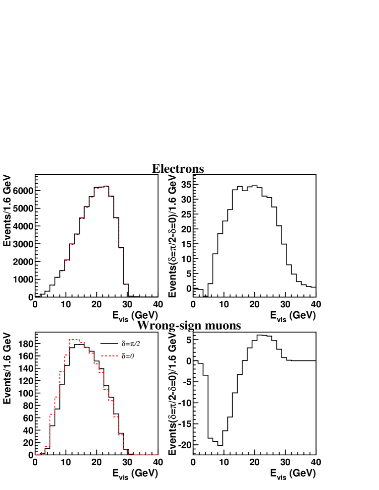
Figure 14: Energy spectra and differences between no CP violation ($\delta$=0) or maximal CP violation ($\delta=\pi/2$). The two upper plots refer to the electron class, the lower ones to the wrong-sign muon class. The plots on the left show the energy spectra for the two cases, the ones on the right the different in number of events as a function of the energy. The helicity of muons circulating in the ring has been chosen in such a way to enhance the effect, i.e. negative muons have been used for the upper plots, and positive ones for the lower plots.

Figure 14 shows for the baseline L=2900 km, the expected visible energy spectra for electron and wrong sing muon class for the two cases $\delta=0$ and $\delta=\pi/2$, and their difference in terms of number of events. As expected, in absolute values, the CP violation affects the two classes in a similar way, but the effect is much more visible and significant for the wrong-sign muons, since the total number of events is smaller.

Figure 14 is normalized to $10^{21}\ \mu^{+}$ decays, since this is the minimum amount of decays required to produce a statistically significant observation of CP violation.

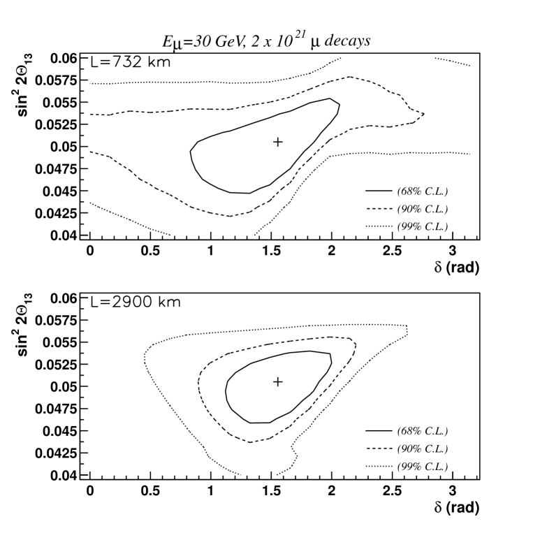
Figure 15: Correlation between $\theta_{13}$ and CP phase $\delta$ for two different baselines and $2\times 10^{21}$ decays.

For the largest baseline $L=7400$ km, CP violation effects are almost undetectable even in case $\delta=\pi/2$ since, wrong sing muon appearance is largely dominated by matter effects. At $L=732$ km, the effect of a non-vanishing $\delta$ is more striking thanks to the higher event rates and the smaller neutrino path in matter. However, as we formerly pointed out, this effect is similar to the one produced by a smaller value of $\theta_{13}$ and therefore, both effects cannot be disentangled with a single measurement at this baseline as shown in figure 15, where the correlations between $\delta$ and $\theta_{13}$ prevent a precise determination of any of them. Nonetheless, a measurement at $L=7400$ km where CP violation effects are negligible and the most accurate determination of $\theta_{13}$ exits, can be combined with data collected at $L=732$ km to produce a precise determination of $\delta$.

Another possibility to unveil the existence of CP violation is to perform a single measurement at $L=2900$ km. As shown in figure 14, at this distance the effect of $\delta\neq 0$ is twofold: not only the event rate is modified but also the spectral shape. This last effect cannot be produced by a change on $\theta_{13}$. Figure 15 shows that at this distance the correlation between $\delta$ and $\theta_{13}$ has diminished and therefore a better determination of the parameters can be achieved with a single measurement.

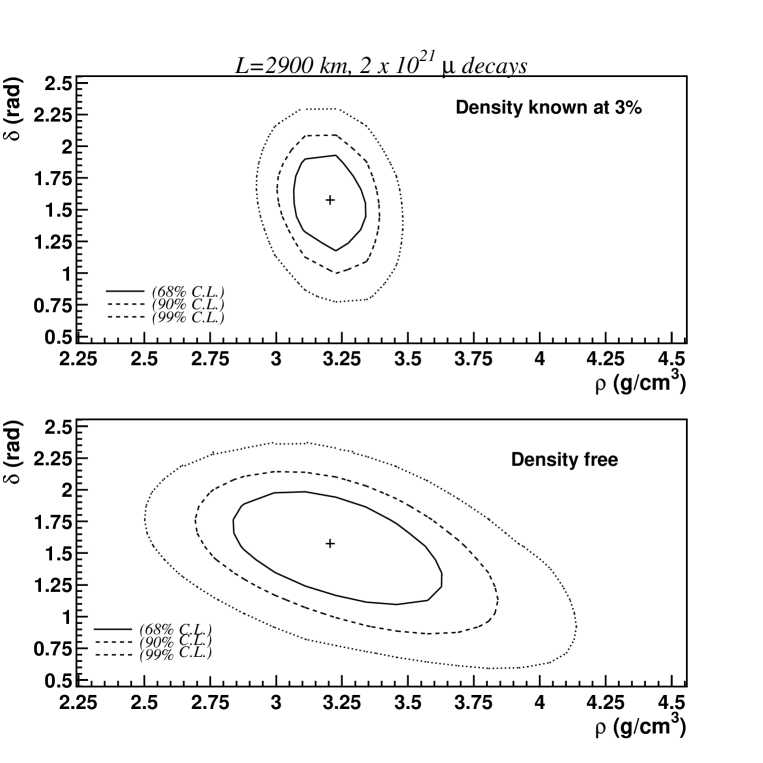
Figure 16: Correlation between the average matter density $\rho$ and the CP phase $\delta$ for L=2900 km. In the lower plot we leave Earth’s mean density as a free parameter in the fit. In the upper plot we assume that density is known within $3\%$. We see that the presence of matter does not spoil the possibility of performing a measurement of $\delta$.

For a baseline of $L=2900$ km, matter effects are not so strong as for the longest baseline. The possibility of measuring the CP-violating phase $\delta$ is not spoiled by the fake asymmetries due to the matter interactions, but both effects, even if correlated, can be measured at the same time. This is shown in figure 16, where the result of a simultaneous fit to the average matter density $\rho$ and the phase $\delta$ is presented for the two cases where $\rho$ is left as a free parameter or it is known beforehand with a $3\%$ accuracy.

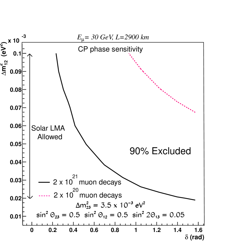
Figure 17: 90%C.L. sensitivity on the CP phase $\delta$ as a function of $\Delta m^{2}_{12}$ for two different normalizations: solid (dashed) line corresponds to $10^{21}\ (10^{20})$ muons decays of each polarity.

Figure 18: Measurement of the CP violating phase $\delta$ for $2\times 10^{21}\ \mu$ decays and $L=2900$ km. The two mass differences and the three mixing angles have been left free during the fit. The reference value is $\delta=\pi/2$. The three curves are obtained using respectively in the fit all classes, only the muon classes, or only electrons and NC-like events.

In case no CP violation is observed, the allowed $\delta$ values at 90$\%$ C.L. as a function of $\Delta m^{2}_{12}$ are shown in figure 17 for two different muon normalizations. On the other hand, if a significant effect is detected, the precision achievable on the measurement of the CP phase $\delta$ is shown in figure 18. We fit $\delta$ using all event classes, leaving the five parameters governing the oscillation free. Assuming a reference value of $90^{o}$ for $\delta$ and $10^{21}$ muon decays of each polarity, we get: $90\pm 15^{o}$. Therefore a precision around 20$\%$ is expected. Finally, we note that the change on the expected precision for $\theta_{13}$ is negligible when $\Delta m^{2}_{12}$ and $\theta_{12}$ are included in the fit.

10.3 Use of quasi-elastic events

Quasi-elastic events can also be useful to spot the presence of CP violation. Table 8 shows the expected number of QE electron events after kinematics cuts (a back to back electron-proton final state with proton kinetic energy in excess of 100 MeV). Three different assumptions for the total number of muon decays and the baseline of 2900 km have been assumed. In case CP is conserved, we expect 35 (96) quasi-elastic electron events for $\Delta m^{2}_{32}=3.5(7)\times 10^{-3}$ eV² and $10^{21}$ muon decays of each polarity. In case $\delta=\pi/2$, we expect 26 and 85 events for the two mass differences considered. The effect is at the one sigma level. To obtain a statistically conclusive signal for CP violation would require more than $10^{21}$ muon decays.

CP-violation with quasi-elastic events
L=2900 km		$N_{ele}$	$N_{ele}$	Stat.
		$(\delta=0)$	$(\delta=\pi/2)$	significance
$\Delta m^{2}_{32}=3.5\times 10^{-3}eV^{2}$	$10^{21}$ $\mu^{\pm}$	35	26	$1.5\sigma$
$\sin^{2}\theta_{23}=0.5$, $\sin^{2}2\theta_{23}=0.05$	$5\times 10^{21}$ $\mu^{\pm}$	175	130	$3.4\sigma$
$\Delta m^{2}_{12}=10^{-4}$ eV2, $\sin^{2}\theta_{12}=0.5$	$10^{22}$ $\mu^{\pm}$	350	260	$4.8\sigma$
$\Delta m^{2}_{32}=7\times 10^{-3}$ eV2	$10^{21}$ $\mu^{\pm}$	96	85	$1.1\sigma$
$\sin^{2}\theta_{23}=0.5$, $\sin^{2}2\theta_{23}=0.05$	$5\times 10^{21}$ $\mu^{\pm}$	480	425	$2.5\sigma$
$\Delta m^{2}_{12}=10^{-4}$ eV2, $\sin^{2}\theta_{12}=0.5$	$10^{22}$ $\mu^{\pm}$	960	850	$3.6\sigma$

Table 8: Expected QE electron events ($N_{ele}$) at a baseline of 2900 km in case there is no CP violation and in case CP violation phase in vacuum is maximal. The last column shows, in number of sigmas, the statistical significance expected for the QE electron sample in case CP is violated in the lepton sector.

11 Conclusions

In this paper, we tried to understand in deeper detail the capabilities an experiment at the Neutrino Factory, with the aim of exploiting as much as possible the possibility of studying several neutrino transitions at the same time. For this reason, we have considered as a baseline detector a large Liquid Argon TPC with external muon identifier, the most versatile design proposed so far for large neutrino experiments.

Assuming an oscillation scenario favoured by present experimental results, the leading oscillation would be between the second and third neutrino family, which are maximally mixed. Therefore, a very precise determination of the parameters governing this transition, $\theta_{23}$ and $\Delta m^{2}_{23}$ is essential also for the understanding of all other processes. This is mainly achieved using the information coming from the $\nu_{\mu}$ disappearance (right-sign muon class), provided that the baseline and beam energy are chosen in such a way that the first oscillation maximum is visible as a dip in the oscillated spectrum.

The maximal sensitivity to $\theta_{13}$ is achieved for very small background levels, since we are looking in this case for small signals; most of the information is coming from the clean wrong-sign muon class, and from quasi-elastic events.

On the other hand, if its value is not too small, for a measurement of $\theta_{13}$, the signal/background ratio could be not so crucial, and also the other event classes can contribute to this measurement.

Like for a B-Factory, a $\nu$-Factory should have among its aims the overconstraining of the oscillation pattern, in order to look for unexpected new physics effects. This can be achieved in global fits of the parameters, where the unitarity of the mixing matrix is not strictly assumed. Using a detector able to identify the $\tau$ lepton production via kinematic means, it is possible to verify the unitarity in $\nu_{\mu}\rightarrow\nu_{\tau}$ and $\nu_{e}\rightarrow\nu_{\tau}$ transitions. For this latter, the possibility of a kinematical $\tau$ identification for wrong-sign muon events could allow for the first time a clear identification of this type of oscillations.

The study of CP violation in the lepton system is a very fascinating subject, and probably the most ambitious goal of this kind of machines. It will only be possible for high beam intensities, and if the parameters governing the solar neutrino deficit are in the region usually indicated as large mixing angle MSW solution. Matter effect can mimic CP violation; however, a multiparameter fit at the right baseline can allow a simultaneous determination of matter and CP-violating parameters.

Also for CP-violation measurements most of the information would come from the wrong-sign muon class, but since in this case the electron class would also be affected, the study of these events (and of the very clean quasi-elastic interactions) can provide essential cross-checks for these delicate measurements.

Appendix A Oscillations in matter

In reference [23], the authors compute analytic expressions for the mass eigenvalues, mixing angles and CP-violation phase in matter, assuming the mixing matrix $U$ is parametrized “à la CKM”. Since several missprints were observed, we reproduce here the corrected expressions:

For neutrinos, the mass eigenvalues in matter $M_{1},\ M_{2}$ and $M_{3}$ are:

$$M_{1}^{2} = m_{1}^{2}+\frac{A}{3}-\frac{1}{3}\sqrt{A^{2}-3B}S-\frac{\sqrt{3}}{3}\sqrt{A^{2}-3B}\sqrt{1-S^{2}}$$ (34)

$$M_{2}^{2} = m_{1}^{2}+\frac{A}{3}-\frac{1}{3}\sqrt{A^{2}-3B}S+\frac{\sqrt{3}}{3}\sqrt{A^{2}-3B}\sqrt{1-S^{2}}$$ (35)

$$M_{3}^{2} = m_{1}^{2}+\frac{A}{3}+\frac{2}{3}\sqrt{A^{2}-3B}S$$ (36)

where

$$A = \Delta m^{2}_{21}+\Delta m^{2}_{31}+D$$ (37)

$$B = \Delta m^{2}_{21}\Delta m^{2}_{31}+D[\Delta m^{2}_{31}c^{2}_{13}+\Delta m^{2}_{21}(c^{2}_{13}c^{2}_{12}+s^{2}_{13})]$$ (38)

$$C = D\Delta m^{2}_{21}\Delta m^{2}_{31}c^{2}_{13}c^{2}_{12}$$ (39)

$$D = 2\sqrt{2}G_{F}N_{e}E\rm\ for\ neutrinos$$ (40)

$$S = \cos\left[\frac{1}{3}\arccos\left(\frac{2A^{3}-9AB+27C}{2\sqrt{(A^{2}-3B)^{3}}}\right)\right]$$ (41)

and $c_{ij}=\cos\theta_{ij}$ and $s_{ij}=\sin\theta_{ij}$. The mixing angles and CP phase in matter are:

$$\sin^{2}\theta^{m}_{12} = \frac{-(M_{2}^{4}-\alpha M_{2}^{2}+\beta)\Delta M^{2}_{31}}{\Delta M^{2}_{32}(M_{1}^{4}-\alpha M_{1}^{2}+\beta)-\Delta M^{2}_{31}(M^{4}_{2}-\alpha M_{2}^{2}+\beta)}$$ (42)

$$\sin^{2}\theta^{m}_{13} = \frac{M_{3}^{4}-\alpha M_{3}^{2}+\beta}{\Delta M^{2}_{31}\Delta M^{2}_{32}}$$ (43)

$$\sin^{2}\theta^{m}_{23} = \frac{G^{2}s^{2}_{23}+F^{2}c^{2}_{23}+2GFc_{23}s_{23}c_{\delta}}{G^{2}+F^{2}}$$ (44)

$$e^{-i\delta_{m}} = \frac{(G^{2}e^{-i\delta}-F^{2}e^{i\delta})s_{23}c_{23}+GF(c^{2}_{23}-s^{2}_{23})}{\sqrt{(G^{2}s^{2}_{23}+F^{2}c^{2}_{23}+2GFc_{23}s_{23}c_{\delta})(G^{2}c^{2}_{23}+F^{2}s^{2}_{23}-2GFc_{23}s_{23}c_{\delta})}}$$ (45)

where

$$\alpha = m_{3}^{2}c^{2}_{13}+m_{2}^{2}(c^{2}_{13}c^{2}_{12}+s^{2}_{13})+m_{1}^{2}(c^{2}_{13}s^{2}_{12}+s^{2}_{13})$$ (46)

$$\beta = m_{3}^{2}c^{2}_{13}(m_{2}^{2}c^{2}_{12}+m_{1}^{2}s^{2}_{12})+m_{2}^{2}m_{1}^{2}s^{2}_{13}$$ (47)

$$G = [\Delta m^{2}_{31}(M_{3}^{2}-m_{1}^{2}-\Delta m^{2}_{21})-\Delta m^{2}_{21}(M_{3}^{2}-m_{1}^{2}-\Delta m^{2}_{31})s^{2}_{12}]c_{13}s_{13}$$ (48)

$$F = (M_{3}^{2}-m_{1}^{2}-\Delta m^{2}_{31})\Delta m^{2}_{21}c_{12}s_{12}c_{13}$$ (49)

For anti-neutrinos, we must replace $D$ by $-D$.

In the case of one-mass scale approximation, the oscillation probabilities are simply The oscillation probabilities are:

$$P({\nu_{e}}\rightarrow{\nu_{e}},E,L) = 1-\sin^{2}(2\theta^{m}_{13})\Delta^{2}_{32}$$ (50)

$$P({\nu_{e}}\rightarrow{\nu_{\mu}},E,L) = \sin^{2}(2\theta^{m}_{13})\sin^{2}(\theta^{m}_{23})\Delta^{2}_{32}$$

$$P({\nu_{e}}\rightarrow{\nu_{\tau}},E,L) = \sin^{2}(2\theta^{m}_{13})\cos^{2}(\theta^{m}_{23})\Delta^{2}_{32}$$

$$P({\nu_{\mu}}\rightarrow{\nu_{\mu}},E,L) = 1-4\cos^{2}(\theta^{m}_{13})\sin^{2}(\theta^{m}_{23})\left[1-\cos^{2}(\theta^{m}_{13})\sin^{2}(\theta^{m}_{23})\right]\Delta^{2}_{32}$$

$$P({\nu_{\mu}}\rightarrow{\nu_{\tau}},E,L) = \cos^{4}(\theta^{m}_{13})\sin^{2}(2\theta^{m}_{23})\Delta^{2}_{32}$$

where $\Delta^{2}_{32}=\sin^{2}\left((M_{3}^{2}-M_{2}^{2})L/4E\right)$.

References

-
[1]
Y. Fukuda et al. [Super-Kamiokande Collaboration],
Phys. Lett. B 433 (1998) 9.
C.W. Walter, invited talk, on behalf of the Super-Kamiokande Collab., at International Europhysics Conference on High-Energy Physics (EPS-HEP 99), Tampere, Finland, 15-21 Jul 1999. - [2] B. Pontecorvo, J. Exptl. Theoret. Phys. 33, 549 (1957) [Sov. Phys. JETP 6, 429 (1958)]; B. Pontecorvo, J. Exptl. Theoret. Phys. 34, 247 (1958) [Sov. Phys. JETP 7, 172 (1958)]; Z. Maki, M. Nakagawa and S. Sakata, Prog. Theor. Phys. 28 (1962) 870; B. Pontecorvo, J. Expt. Theor. Phys 53 (1967) 1717; V. Gribov and B. Pontecorvo, Phys. Lett. B 28, 493 (1969).
-
[3]
“E362 Proposal for a long baseline neutrino oscillation experiment,
using KEK-PS and Super-Kamiokande”, February 1995.
H. W. Sobel, proceedings of Eighth International Workshop on Neutrino Telescopes, Venice 1999, vol 1 pg 351. -
[4]
E. Ables et al.[MINOS Collaboration],
“P-875: A Long baseline neutrino oscillation experiment at Fermilab,”
FERMILAB-PROPOSAL-P-875.
The MINOS detectors Technical Design Report, NuMI-L-337, October 1998. - [5] K. Kodama et al.[OPERA Collaboration], “OPERA: a long baseline appearance experiment in the CNGS beam from CERN to Gran Sasso”, CERN/SPSC 99-20 SPSC/M635 LNGS-LOI 19/99.
- [6] F. Arneodo et al.[ICARUS and NOE Collaboration], “ICANOE: Imaging and calorimetric neutrino oscillation experiment,” LNGS-P21/99, INFN/AE-99-17, CERN/SPSC 99-25, SPSC/P314; F. Cavanna et al.[ICANOE Collaboration], “ICANOE: Answers to questions and remarks concerning the ICANOE project,” LNGS-P21/99-ADD2, CERN/SPSC 99-40, SPSC/P314 Add 2; A. Rubbia [ICARUS & NOE collaborations], hep-ex/0001052. Updated information can be found at http://pcnometh4.cern.ch.
- [7] E. Church et al., “A proposal for an experiment to measure muon-neutrino electron- neutrino oscillations and muon-neutrino disappearance at the Fermilab Booster: BooNE,” FERMILAB-P-0898. Updated information on the BOONE proposal can be found at http://www.neutrino.lanl.gov/BooNE/.
- [8] C. Athanassopoulos et al., (LSND Collaboration), Phys. Rev. C 54 (2685) 1996.; C. Athanassopoulos et al.(LSND Collaboration), PRL 77 (3082) 1996.; Phys. Rev. Lett. 75 (2650) 1995.. C. Athanassopoulos et al. [LSND Collaboration], Phys. Rev. Lett. 81, 1774 (1998).
- [9] S. Geer, Phys. Rev. D 57 (1998) 6989.
- [10] Information on the neutrino factory studies and mu collider collaboration at BNL can be found at http://www.cap.bnl.gov/mumu/. Information on the neutrino factory studies at FNAL can be found at http://www.fnal.gov/projects/muon_collider/. Information on the neutrino factory studies at CERN can be found at http://muonstoragerings.cern.ch/Welcome.html/.
- [11] A. Bueno, M. Campanelli and A. Rubbia, hep-ph/9808485 ETHZ-IPP-98-05.
- [12] A. Bueno, M. Campanelli and A. Rubbia, hep-ph/9809252; CERN-EP/98-140.
- [13] A. de Rújula, M. B. Gavela and P. Hernández, Nucl. Phys. B 547 (1999) 21.
- [14] V. Barger, S. Geer, R. Raja and K. Whisnant, hep-ph/9911524 and hep-ph/0003184.
-
[15]
A. Bueno, M. Campanelli and A. Rubbia, hep-ph/9905240, accepted for
publication in Nucl. Phys. B.
V. Barger, S. Geer and K. Whisnant, Phys. Rev. D 61 (2000) 053004.
M. Freund, M. Lindner, S. T. Petcov and A. Romanimo, hep-ph/9912457. -
[16]
A. Donini, M. B. Gavela, P. Hernández and S. Rigolin,
hep-ph/9909254.
M. Koike and J. Sato, hep-ph/9909469.
G. Barenboim and R. Scheck, hep-ph/0001208.
H. Fritzsch and Z. Xing, hep-ph/0002248. - [17] D. A. Harris and A. Para, “Neutrino Oscillation Appearance Experiment using Nuclear Emulsion and Magnetized Iron,”, hep-ex/0001035.
- [18] A. Cervera et al., “Golden measurements at a neutrino factory”, hep-ph/0002108.
- [19] see e.g. P. Lipari, hep-ph/9903481.
-
[20]
L. Wolfenstein, Phys. Rev. D 17 (1978) 2369.
Phys. Rev. D 20 (1979) 2634.
S. P. Mikheyev and A. Yu. Smirnov, Sov. J. Nucl. Phys. 42 (1986) 913. - [21] J.N. Bahcall, P.I. Krastev and A.Y. Smirnov, Phys. Rev. D58, 096016 (1998) hep-ph/9807216 and references therein.
- [22] F.James, MINUIT manual, CERN program libraries p. 43
- [23] H. W. Zaglauer and K. H. Schwarzer, Z. Phys. C 40 (1988) 273.
- [24] V. Barger, K. Whisnant, S. Pakvasa and R. J. N. Phillips, Phys. Rev. D 22 (1980) 2718.
- [25] I. Mocioiu and R. Shrock, hep-ph/0002149.
- [26] M. Apollonio et al.[CHOOZ Collaboration], Phys. Lett. B 466 (1999) 415. Phys. Lett. B 420 (1998) 397.
- [27] G. L. Fogli, E. Lisi and A. Marrone and G. Scioscia, Phys. Rev. D 59 (1999) 033001.
- [28] A. Ferrari and A. Rubbia,”NUX: a neutrino event generator”, ICARUS internal note in preparation.
- [29] A. Ferrari and P.R. Sala, Trieste, ATLAS internal note ATL-PHYS-97-113, Proc. of the Workshop on Nuclear Reaction Data and Nuclear Reactors Physics, Design and Safety, ICTP, Miramare-Trieste, Italy, 15 April–17 May 1996, Proceedings published by World Scientific, A. Gandini, G. Reffo eds, Vol. 2, p. 424, (1998).
- [30] S. Baker and R. Cousins, Nucl. Instrum. Methods 221 (1984) 437.