Approximately self-consistent resummations for
the thermodynamics of the quark-gluon plasma:
I. Entropy and density

Abstract

We propose a gauge-invariant and manifestly UV finite resummation of the physics of hard thermal/dense loops (HTL/HDL) in the thermodynamics of the quark-gluon plasma. The starting point is a simple, effectively one-loop expression for the entropy or the quark density which is derived from the fully self-consistent two-loop skeleton approximation to the free energy, but subject to further approximations, whose quality is tested in a scalar toy model. In contrast to the direct HTL/HDL-resummation of the one-loop free energy, in our approach both the leading-order (LO) and the next-to-leading order (NLO) effects of interactions are correctly reproduced and arise from kinematical regimes where the HTL/HDL are justifiable approximations. The LO effects are entirely due to the (asymptotic) thermal masses of the hard particles. The NLO ones receive contributions both from soft excitations, as described by the HTL/HDL propagators, and from corrections to the dispersion relation of the hard excitations, as given by HTL/HDL perturbation theory. The numerical evaluations of our final expressions show very good agreement with lattice data for zero-density QCD, for temperatures above twice the transition temperature.

Contents

toc

I Introduction

Besides its obvious relevance for cosmology, astrophysics or ultra-relativistic heavy ion collisions, the study of QCD at high temperature and/or large baryonic density [1, 2] presents exciting theoretical challenges. It offers opportunity to explore the properties of matter in a regime where, unlike in ordinary hadronic matter, the fundamental fields of QCD—the quarks and gluons— are the dominant degrees of freedom and the fundamental symmetries are explicit.

Unfortunately, analytical tools available for such a study are not many. However, because of asymptotic freedom, the gauge coupling becomes weak at high temperature, which invites us to try a perturbative treatment of the interactions. But explicit perturbative calculations of the QCD free energy at high temperature, which have been pushed in recent years up to the order $\alpha_{s}^{5/2}$ [3, 4], show an extremely poor convergence except for coupling constants as low as $\alpha\lesssim 0.05$, which would correspond to temperatures as high as $\gtrsim 10^{5}T_{c}$. Already the next-to-leading order perturbative correction, the so-called plasmon effect which is of order $\alpha_{s}^{3/2}\propto g^{3}$, signals the inadequacy of the conventional thermal perturbation theory except for very small coupling, because in contrast to the leading-order terms it leads to a free energy in excess of the ideal-gas value.

Lattice results on the other hand show a slow approach of the ideal-gas result from below with deviations of not more than some 10-15% for temperatures a few times the deconfinement temperature. Besides, these results can be accounted for reasonably well by phenomenological fits involving massive “quasiparticles” [5, 6] with masses of the order of the perturbative leading-order thermal masses. This suggests that the failure of ordinary perturbation theory may not be directly related to the non-perturbative phenomena expected at the scale $g^{2}T$ and which cause a breakdown of the loop expansion at order $g^{6}$ and higher [1]. Rather, the quasiparticle fits support the idea that one should be able to give an accurate description of the thermodynamics of the QCD plasma in terms of its (relatively weakly interacting) quasiparticle excitations.

It is worth emphasizing at this stage that, among the relevant degrees of freedom, the soft collective ones, with momenta of order $gT$, are already non-perturbative. Although their leading order contribution $\propto g^{3}$ to the pressure can be easily isolated [1], it does not make much physical sense to regard this contribution as a genuine perturbative correction.

Indeed, to leading order in $g$, the dynamics of the soft modes is described by an effective theory which includes the one-loop thermal fluctuations of the “hard” modes with momenta $\sim T$. The relevant generalization of the Yang-Mills equation reads [7, 8] :

$$D_{\nu}F^{\nu\mu}=\hat{m}_{D}^{2}\int\frac{{\rm d}\Omega}{4\pi}\,\frac{v^{\mu}v^{i}}{v\cdot D}\,E^{i}\equiv\hat{\Pi}_{\mu\nu}^{ab}A_{b}^{\nu}+\frac{1}{2}\,\hat{\Gamma}_{\mu\nu\rho}^{abc}A_{b}^{\nu}A_{c}^{\rho}+\,...$$ (1)

where the induced current in the right hand side describes the polarization of the hard particles by the soft colour fields $A^{\mu}_{a}$ in an eikonal approximation. [In this equation, $\hat{m}_{D}\sim gT$ is the Debye mass, $E_{a}^{i}$ is the soft electric field, $v^{\mu}\equiv(1,\,{\bf v})$, and the angular integral $\int{\rm d}\Omega$ runs over the orientations of the unit vector ${\bf v}$.] This current is non-local and gauge symmetry, which forces the presence of the covariant derivative $D^{\mu}=\partial^{\mu}+igA^{\mu}$ in the denominator of Eq. (1), makes it also non-linear. When expanded in powers of $A^{\mu}_{a}$, it generates an infinite series of non-local self-energy and vertex corrections, known as “hard thermal loops” (HTL) [9, 7]. The latter encompass important physical phenomena, like screening effects and non-trivial dispersion relations for the soft excitations [2, 8] (and references therein). Similar phenomena exist also in the case of soft fermions, which, to leading order in $g$, obey the following generalized Dirac equation [7] (with $\hat{M}\sim gT$ and $\not\!{v}=\gamma_{\mu}v^{\mu}$) :

$$i\!\not\!\!{D}\psi\,=\,\hat{M}^{2}\int\frac{{\rm d}\Omega}{4\pi}\,\frac{\not\!{v}}{i(v\cdot D)}\,\psi\,\equiv\,\hat{\Sigma}\psi+\hat{\Gamma}_{\mu}^{a}A^{\mu}_{a}\psi+\,...$$ (2)

At soft momenta $k\lesssim gT$, all HTL’s are leading order effects, as obvious in Eqs. (1) and (2), and must be consistently resummed. Analogs of HTL’s exist at finite chemical potential $\mu$. In the regime $\mu\gg T$ these are often referred to as “hard dense loops” (HDL).

In traditional perturbative calculations of the thermodynamics performed in imaginary time [2], the HTL’s play almost no role: only the Debye mass $m_{D}^{2}$ needs to be resummed in the static electric gluon propagator [10]. This resummation is responsible for the occurrence of odd powers of $g$ in the perturbative expansion.

Such a simple resummation however may become insufficient whenever a more complete information on the quasiparticles needs to be taken into account. Quite generally, this physical information is contained in the spectral weight $\rho(k_{0},k)$ related to the corresponding propagator by:

$$D(\omega,k) = \int_{-\infty}^{\infty}\frac{{\rm d}k_{0}}{2\pi}\,\frac{\rho(k_{0},k)}{k_{0}-\omega}\,.$$ (3)

In the imaginary time formalism, and for bosonic fields, $\omega=i\omega_{n}\equiv i2\pi nT$ with integer $n$. Clearly, the restriction to the Matsubara mode with $n=0$ retains in the propagator only one moment of the spectral weight. In the HTL approximation, we know that the spectral density is divided into a pole at time-like momenta and a continuum at space-like momenta. While there exist physical observables which can be accurately described in perturbation theory by a single moment of the spectral weight, this does not appear to be the case in the calculations that we shall present and in which the various pieces of the spectral functions contribute in different ways.

In fact, since the thermodynamical functions are dominated by hard degrees of freedom, an important effect of the soft modes will be to induce corrections on the hard quasiparticle dispersion relations. As we shall find, the spectral functions for large momenta will take the approximate form $\rho(\omega,k)\approx\delta(\omega^{2}-k^{2}-m^{2}_{\infty})$, where $m^{2}_{\infty}\sim g^{2}T^{2}$ is the leading-order thermal mass (or asymptotic mass) of the hard excitation. Clearly, such an effect does not naturally emerge in a scheme where one resums just the $n=0$ Matsubara mode.

In order to overcome all these limitations, it has been recently proposed to perform full resummations of the HTL self-energies $\Pi_{\mu\nu}$ and $\Sigma$ in calculations of the thermodynamical functions. In Refs. [11, 12], this has been done by merely replacing the free propagators by the corresponding HTL-resummed ones in the expression of the free-energy of the ideal gas; e.g. (in simplified notations) :

$${\,\mathrm{T}r\,}\log D_{0}^{-1}\longrightarrow{\,\mathrm{T}r\,}\log(D^{-1}_{0}+\Pi)\,.$$ (4)

In principle, this is just the first step in a systematic procedure which consists in resumming the HTL’s by adding and subtracting them to the tree-level QCD Lagrangian. This would be the extension to QCD of the so-called “screened perturbation theory”[13, 14], a method which, for scalar field theories, has shown an improved convergence (in one- and two-loop calculations) as compared to the straightforward perturbative expansion. But in its zeroth order approximation in Eq. (4), this method over-includes the leading-order interaction term $\propto g^{2}$ (while correctly reproducing the order-$g^{3}$ contribution), and gives rise to new, ultimately temperature-dependent UV divergences and associated additional renormalization scheme dependences.

Another drawback of such a direct HTL resummation appears to be that the HTL’s are kept in the hard momentum regime where they are no longer describing actual physics, while hard momenta are providing the dominant contributions to the thermodynamic potential.

Our approach on the other hand [15, 16] will be based on self-consistent approximations using the skeleton representation of the thermodynamic potential [17] which takes care of overcounting problems automatically, without the need for thermal counterterms. We shall mainly consider the so-called 2-loop-$\Phi$-derivable [18] approximation, for which it turns out that the first derivatives of the thermodynamic potential, the entropy and the quark densities, take a rather simple, effectively one-loop form[19, 20], but in terms of fully dressed propagators.

In gauge theories, the generalized gap equations that determine these dressed propagators are too complicated to be solved exactly (even numerically). But an exact solution would anyhow be unsatisfactory because $\Phi$-derivable approximations in general do not respect gauge invariance. We therefore propose gauge independent but only approximately self-consistent dressed propagators as obtained from (HTL) perturbation theory. Using these in the entropy expression obtained from the 2-loop-$\Phi$-derivable approximation gives a gauge-independent and UV finite approximation for the entropy, which, while being nonperturbative in the coupling, contains the correct leading-order (LO) and the next-to-leading order (NLO) effects of interactions in accordance with thermal perturbation theory. Both turn out to arise from kinematical regimes where the HTL’s are justifiable approximations.

While also being effectively a resummed one-loop expression, the approximately self-consistent entropy differs from the direct HTL-resummation of the free energy in Eq. (4) in that it includes correctly also the LO interaction effects. Remarkably, in our approach the latter are entirely determined by the (asymptotic) thermal masses of the hard excitations. This agrees with and justifies the simple quasiparticle models of Ref. [5, 6], which assume constant masses equal to the respective asymptotic thermal masses for quarks and as many (scalar) bosons as there are transverse gluons. Whereas these models do not include the correct NLO (plasmon) effect, our approach does, but in a rather unconventional manner which demonstrates the nontriviality of the resummation that has been achieved: only part of the plasmon effect is coming directly from soft excitations; a larger part arises from corrections to the dispersion relation of the (dominant) hard excitations by soft modes, as determined by standard HTL perturbation theory [9].

Because of the approximations that we have made, it does matter whether the entropy or the thermodynamic potential is considered. Our approach however attempts to take advantage of the fact that entropy is generally the simpler quantity. Indeed, the way by which the LO and NLO interaction contributions can be traced to spectral properties of free quasiparticles within our entropy expressions indicates a posteriori the adequateness of this particular resummation scheme to the physics contained in the HTL propagators.

The present paper is organized as follows: In Sect. II, the general formalism of $\Phi$-derivable self-consistent approximations is reviewed and the central, effectively one-loop formula for the entropy in a two-loop skeleton approximation to the thermodynamic potential is derived in a scalar theory with cubic and quartic interactions. In the simple solvable model of large-$N$ scalar O($N$) theory [21, 22], where the two-loop $\Phi$-derivable approximation becomes exact, the further approximations that will be considered in the QCD case are compared with the exact solution and their renormalization scale dependence is exhibited.

In Sect. III, the approximately self-consistent resummations are introduced for purely gluonic QCD first, and equivalence with conventional perturbation theory up to and including order $g^{3}$ is proved and analyzed in detail. Sect. IV generalizes this to QCD with quarks and to the quark density as an additional thermodynamic quantity. Some of the more technical details of how the plasmon effect arises in our approach are relegated to the Appendix.

In Sect. V, the various approximations are evaluated numerically. We find that the plasmon effect, which is largely responsible for the poor convergence properties of conventional thermal perturbation theory, in our approach leads only to moderate contributions when compared with the leading-order effects. When combined with a two-loop renormalization group improvement, our results are found to compare remarkably well with available lattice data for temperatures above twice the deconfinement temperature. Moreover, we also present numerical results for the quark density at zero temperature and large chemical potential.

II General formalism. The scalar field

In this section we develop the formalism of propagator renormalization using techniques that allow systematic rearrangements of the perturbative expansion avoiding double-countings. We shall recall in particular how self-consistent approximations can be used to obtain a simple expression for the entropy which isolates the contribution of the elementary excitations as a leading contribution. To get familiarity with the formalism, we demonstrate some of its important features with the example of the scalar field. This provides, in particular, a test of the validity of approximations which will be used in dealing with QCD in the rest of the paper.

A Skeleton expansion for thermodynamical potential and entropy

The thermodynamic potential $\Omega=-PV$ of the scalar field can be written as the following functional of the full propagator $D$ [17, 18]:

$$\beta\Omega[D]=-\log Z={1\over 2}{\,\mathrm{T}r\,}\log D^{-1}-{1\over 2}{\,\mathrm{T}r\,}\Pi D+\Phi[D]\,,$$ (5)

where ${\,\mathrm{T}r\,}$ denotes the trace in configuration space, $\beta=1/T$, $\Pi$ is the self-energy related to $D$ by Dyson’s equation ($D_{0}$ denotes the bare propagator):

$$D^{-1}=D^{-1}_{0}+\Pi,$$ (6)

and $\Phi[D]$ is the sum of the 2-particle-irreducible “skeleton” diagrams

$$-\Phi[D]=\epsfbox[50390550430]{phi.ps}$$ (7)

The essential property of the functional $\Omega[D]$ is to be stationary under variations of $D$ (at fixed $D_{0}$) around the physical propagator. The physical pressure is then obtained as the value of $\Omega[D]$ at its extremum. The stationarity condition,

$${\delta\Omega[D]/\delta D}=0,$$ (8)

implies the following relation

$$\delta\Phi[D]/\delta D={1\over 2}\Pi,$$ (9)

which, together with Eq. (6), defines the physical propagator and self-energy in a self-consistent way. Eq. (9) expresses the fact that the skeleton diagrams contributing to $\Pi$ are obtained by opening up one line of a two-particle-irreducible skeleton. Note that while the diagrams of the bare perturbation theory, i.e., those involving bare propagators, are counted once and only once in the expression of $\Pi$ given above, the diagrams of bare perturbation theory contributing to the thermodynamic potential are counted several times in $\Phi$. The extra terms in Eq. (5) precisely correct for this double-counting.

Self-consistent (or variational) approximations, i.e., approximations which preserve the stationarity property (8), are obtained by selecting a class of skeletons in $\Phi[D]$ and calculating $\Pi$ from Eq. (9). Such approximations are commonly called “$\Phi$-derivable” [18].

The traces over configuration space in Eq. (5) involve integration over imaginary time and over spatial coordinates. Alternatively, these can be turned into summations over Matsubara frequencies and integrations over spatial momenta:

$$\int_{0}^{\beta}{\rm d}\tau\int{\rm d}^{3}x\rightarrow\beta V\int[{\rm d}k],$$ (10)

where $V$ is the spatial volume, $k^{\mu}=(i\omega_{n},{\bf k})$ and $\omega_{n}=n\pi T$, with $n$ even (odd) for bosonic (fermionic) fields (the fermions will be discussed later). We have introduced a condensed notation for the the measure of the loop integrals (i.e., the sum over the Matsubara frequencies $\omega_{n}$ and the integral over the spatial momentum ${\bf k}$):

$$\int[{\rm d}k]\equiv T\sum_{n,even}\int\frac{{\rm d}^{3}k}{(2\pi)^{3}}\,,\qquad\,\,\,\,\int\{{\rm d}k\}\equiv T\sum_{n,odd}\int\frac{{\rm d}^{3}k}{(2\pi)^{3}}\,.$$ (11)

Strictly speaking, the sum-integrals in equations like Eq. (5) contain ultraviolet divergences, which requires regularization (e.g., by dimensional continuation). Since, however, most of the forthcoming calculations will be free of ultraviolet problems (for the reasons explained at the end of this subsection), we do not need to specify here the UV regulator (see however Sect. II B for explicit calculations).

For the purpose of developing approximations for the entropy it is convenient to perform the summations over the Matsubara frequencies. One obtains then integrals over real frequencies involving discontinuities of propagators or self-energies which have a direct physical significance. Using standard contour integration techniques, one gets:

$$\Omega/V=\int\!\!{d^{4}k\over(2\pi)^{4}}\,n(\omega)\left({\,\mathrm{I}m\,}\log(-\omega^{2}+k^{2}+\Pi)-{\,\mathrm{I}m\,}\Pi D\right)+T\Phi[D]/V$$ (12)

where $n(\omega)=1/({\rm e}^{\beta\omega}-1)$.

The analytic propagator $D(\omega,k)$ can be expressed in terms of the spectral function:

$$D(\omega,k)=\int_{-\infty}^{\infty}{dk_{0}\over 2\pi}{\rho(k_{0},k)\over k_{0}-\omega}.$$ (13)

and we define, for $\omega$ real,

$${\,\mathrm{I}m\,}D(\omega,k)\equiv{\,\mathrm{I}m\,}D(\omega+i\epsilon,k)=\frac{\rho(\omega,k)}{2}.$$ (14)

The imaginary parts of other quantities are defined similarly.

We are now in the position to calculate the entropy density:

$${\cal S}=-{\partial(\Omega/V)/\partial T}\,.$$ (15)

The thermodynamic potential, as given by Eq. (12) depends on the temperature through the statistical factors $n(\omega)$ and the spectral function $\rho$, which is determined entirely by the self-energy. Because of Eq. (8) the temperature derivative of the spectral density in the dressed propagator cancels out in the entropy density and one obtains [19, 20]:

$${\cal S} = -\int\!\!{d^{4}k\over(2\pi)^{4}}{\partial n(\omega)\over\partial T}{\,\mathrm{I}m\,}\log D^{-1}(\omega,k)$$ (17)

$$+\int\!\!{d^{4}k\over(2\pi)^{4}}{\partial n(\omega)\over\partial T}{\,\mathrm{I}m\,}\Pi(\omega,k){\,\mathrm{R}e\,}D(\omega,k)+{\cal S}^{\prime}$$

with

$${\cal S}^{\prime}\equiv-{\partial(T\Phi)\over\partial T}\Big{|}_{D}+\int\!\!{d^{4}k\over(2\pi)^{4}}{\partial n(\omega)\over\partial T}{\,\mathrm{R}e\,}\Pi{\,\mathrm{I}m\,}D.$$ (18)

We shall verify explicitly that for the two-loop skeletons, we have:

$${\cal S}^{\prime}=0.$$ (19)

Loosely speaking, the first two terms in Eq. (17) represent essentially the entropy of “independent quasiparticles”, while ${\cal S}^{\prime}$ accounts for a residual interaction among these quasiparticles [20].

Since the condition (19) plays an important role in our work, we shall derive it explicitly in a scalar model with interaction term

$${\cal L}_{int}=(g/3!)\phi^{3}-(\lambda/4!)\phi^{4},$$

which is a simple toy model of the tri- and quadrilinear self-interactions of gauge bosons. (Interactions with fermions are already covered by the analysis contained in Ref. [20].) In the two-loop approximation, where only the first two diagrams of the skeletons in Eq. (7) are kept, the contribution involving two 3-vertices reads

$$-T\Phi^{(a)}={g^{2}\over 12}T^{2}\sum_{\omega_{1},\omega_{2}}\int{d^{3}k_{1}\,d^{3}k_{2}\over(2\pi)^{6}}D(\omega_{1},|\vec{k}_{1}|)D(\omega_{2},|\vec{k}_{2}|)D(-\omega_{1}-\omega_{2},|-\vec{k}_{1}-\vec{k}_{2}|).$$ (20)

Expressing the propagators in terms of the spectral functions, and evaluating the Matsubara sums by contour integration, one gets:

$$-T\Phi^{(a)} = {g^{2}\over 12}\int{d^{4}k\,d^{4}k^{\prime}\,d^{4}k^{\prime\prime}\over(2\pi)^{9}}\delta^{3}(\vec{k}+\vec{k}^{\prime}+\vec{k}^{\prime\prime})\rho(k)\rho(k^{\prime})\rho(k^{\prime\prime}){\bf P}{1\over k_{0}+k_{0}^{\prime}+k_{0}^{\prime\prime}}$$ (22)

$$\qquad\times\left\{[n(k_{0})+1][n(k_{0}^{\prime})+n(k_{0}^{\prime\prime})+1]+n(k_{0}^{\prime})n(k_{0}^{\prime\prime})\right\}$$

where P denotes the principal value prescription and we have used the identity:

$$n(x+y)[1+n(x)+n(y)]=n(x)n(y)\,.$$ (23)

The two-loop skeleton involving the 4-vertex is given by the simpler expression

$$-T\Phi^{(b)}=-{\lambda\over 8}\left[\sum_{\omega}\int\!\!{d^{3}k\over(2\pi)^{3}}D(\omega,k)\right]^{2}\\ =-{\lambda\over 8}\int{d^{4}k\,d^{4}k^{\prime}\over(2\pi)^{8}}\rho(k)\rho(k^{\prime})\left\{n(k_{0})n(k^{\prime}_{0})\right\}.$$ (24)

According to Eq. (18), the first contribution to ${\cal S}^{\prime}$ is given by differentiating Eqs. (22) and (24) with respect to $T$ at fixed $\rho$. Because the integrand in front of the curly brackets in (22) is symmetric, the arguments of the distribution functions can be freely exchanged as long as the fact that their products come with distinct arguments is preserved. $\partial_{T}[-T\Phi]$ is therefore obtained by replacing the terms in curly brackets in (22) by $\{6n(k_{0}^{\prime})\partial_{T}n(k_{0})+3\partial_{T}n(k_{0})]\}$ and that in (24) by $2n(k_{0}^{\prime})\partial_{T}n(k_{0})$.

The second contribution to ${\cal S}^{\prime}$ involves the real part of the self-energy as given by the two (dressed) one-loop diagrams following from opening up one line in the first two diagrams in (7),

$${\,\mathrm{R}e\,}\,\Pi^{(a)}(\omega,q) = -{g^{2}\over 2}\int\!\!{d^{3}k\over(2\pi)^{3}}\int\!{dk_{0}\over 2\pi}{dk_{0}^{\prime}\over 2\pi}\rho(k_{0},|\vec{k}|)\rho(k_{0}^{\prime},|\vec{k}+\vec{q}|)$$ (26)

$$\qquad\times[n(k_{0})+n(k_{0}^{\prime})+1]{\bf P}{1\over\omega+k_{0}+k_{0}^{\prime}}$$

$${\,\mathrm{R}e\,}\,\Pi^{(b)} = {\lambda\over 2}\int\!\!{d^{4}k\over(2\pi)^{4}}n(k_{0})\rho(k_{0},k)$$ (27)

This gives

$$\int\!\!{d^{4}k\over(2\pi)^{4}}{\partial n(k_{0})\over\partial T}{\,\mathrm{R}e\,}\Pi^{(a)}{\,\mathrm{I}m\,}D = -{1\over 4}\int\!{d^{4}k\,d^{4}k^{\prime}\,d^{4}k^{\prime\prime}\over(2\pi)^{9}}\delta^{3}(\vec{k}+\vec{k}^{\prime}+\vec{k}^{\prime\prime})\rho(k)\rho(k^{\prime})\rho(k^{\prime\prime})$$ (29)

$$\qquad\times{\bf P}{1\over k_{0}+k_{0}^{\prime}+k_{0}^{\prime\prime}}[\partial_{T}n(k_{0})][n(k_{0}^{\prime})+n(k_{0}^{\prime\prime})+1]$$

$$\int\!\!{d^{4}k\over(2\pi)^{4}}{\partial n(k_{0})\over\partial T}{\,\mathrm{R}e\,}\Pi^{(b)}{\,\mathrm{I}m\,}D = \int\!\!{d^{4}k\over(2\pi)^{4}}{\partial n(k_{0})\over\partial T}{\rho(k)\over 2}{\lambda\over 2}\int\!\!{d^{4}k^{\prime}\over(2\pi)^{4}}n(k_{0}^{\prime})\rho(k^{\prime})$$ (30)

where we have used ${\,\mathrm{I}m\,}D=\rho/2$. Indeed, this cancels precisely $-\partial_{T}[T\Phi]$ as obtained above, verifying the proposition that ${\cal S}^{\prime}=0$ for the lowest-order (two-loop) diagrams in $\Phi[D]$.

As the previous derivation shows, the vanishing of ${\cal S}^{\prime}$ holds whether the propagator are the self-consistent propagators or not. That is, only the relation (9) is used, and the proof does not require $D$ to satisfy the self-consistent Dyson equation (6). A general analysis of the contributions to ${\cal S}^{\prime}$ and their physical interpretation can be found in Ref. [23].

We emphasize now a few attractive features of Eq. (17) with ${\cal S}^{\prime}=0$, which makes the entropy a privileged quantity to study the thermodynamics of ultrarelativistic plasmas. We note first that the formula for $\cal S$ at 2-loop order involves the self-energy only at 1-loop order. Besides this important simplification, this formula for ${\cal S}$, in contrast to the pressure, has the advantage of manifest ultra-violet finiteness, since ${\partial n/\partial T}$ vanishes exponentially for both $\omega\to\pm\infty$. Also, any multiplicative renormalization $D\to ZD$, $\Pi\to Z^{-1}\Pi$ with real $Z$ drops out from Eq. (17). Finally, the entropy has a more direct quasiparticle interpretation than the pressure. This will be illustrated explicitly in the simple model of the next subsection. More generally, Eq. (17) can be transformed with the help of the following identity:

$${\,\mathrm{I}m\,}\log D^{-1}(\omega,k)=\arctan\left(\frac{{\,\mathrm{I}m\,}\Pi}{{\,\mathrm{R}e\,}D^{-1}}\right)-\pi\epsilon(\omega)\theta(-{\,\mathrm{R}e\,}D^{-1}),$$ (31)

with $\epsilon(\omega)$ the sign function and $-{\pi\over 2}<\arctan(x)<{\pi\over 2}$. Using this identity we rewrite ${\cal S}$ as ${\cal S}={\cal S}_{pole}+{\cal S}_{damp}$, with

$${\cal S}_{pole} = \int\!\!{d^{4}k\over(2\pi)^{4}}{\partial n(\omega)\over\partial T}\pi\epsilon(\omega)\theta(-{{\,\mathrm{R}e\,}}D^{-1}(\omega,k))$$ (32)

$$= \int\!\!{d^{3}k\over(2\pi)^{3}}\Bigl{\{}(1+n_{k})\log(1+n_{k})\,-\,n_{k}\log n_{k}\Bigr{\}}.$$ (33)

To get the second line, we have made an integration by part, using

$$\frac{\partial n(\omega)}{\partial T}=-\,{\partial\sigma(\omega)\over\partial\omega},\qquad\sigma(\omega)\equiv-n\log n+(1+n)\log(1+n),$$ (34)

and we have set $n_{k}\equiv n(\epsilon_{k})$, with $\epsilon_{k}$ solution of ${\,\mathrm{R}e\,}D^{-1}(\omega=\varepsilon_{k},k)=0$. The quasiparticles thus defined by the poles of the propagator are sometimes called “dynamical quasiparticles” [23]. The quantity ${\cal S}_{pole}$ is the entropy of a system of such non-interacting quasiparticles, while the quantity

$${\cal S}_{damp}=\int\!\!{d^{4}k\over(2\pi)^{4}}{\partial n(\omega)\over\partial T}\left[{\rm Im}\Pi(\omega,k){\,\mathrm{R}e\,}D(\omega,k)-\arctan\left(\frac{{\,\mathrm{I}m\,}\Pi}{{\,\mathrm{R}e\,}D^{-1}}\right)\right],$$ (35)

which vanishes when ${\,\mathrm{I}m\,}\Pi$ vanishes, is a contribution coming from the continuum part of the quasiparticle spectral weights.

B A simple model

In this section we shall present the self-consistent solution for the $(\lambda/4!)\phi^{4}$ theory, keeping in $\Phi$ only the two-loop skeleton whose explicit expression is given in Eq. (24). Anticipating the fact that the fully dressed propagator will be that of a massive particle, we write the spectral function as $\rho(k_{0},{\bf k})=2\pi\,\epsilon(k_{0})\,\delta(k_{0}^{2}-{\bf k}^{2}-m^{2})$, and consider $m$ as a variational parameter. The thermodynamic potential (5), or equivalently the pressure, becomes then a simple function of $m$. By Dyson’s equation, the self-energy is simply $\Pi=m^{2}$. We set:

$$I(m)\,\equiv\,\frac{1}{2}\int[{\rm d}k]\,D(k)\,={1\over 2}\int[{\rm d}k]\,\frac{1}{\omega_{n}^{2}+{\bf k}^{2}+m^{2}}.$$ (36)

Then the pressure can be written as:

$$-P=\frac{\Omega}{V}=\frac{1}{2}\int\frac{{\rm d}^{3}k}{(2\pi)^{3}}\,\varepsilon_{k}+\frac{1}{\beta}\int\frac{{\rm d}^{3}k}{(2\pi)^{3}}\,\log(1-{\rm e}^{-\beta\varepsilon_{k}})-m^{2}I(m)+\frac{\lambda_{0}}{2}\,I^{2}(m),$$ (37)

where $\varepsilon_{k}^{2}\equiv k^{2}+m^{2}$. By demanding that $P$ be stationary with respect to $m$ one obtains the self-consistency condition which takes here the form of a “gap equation”:

$$m^{2}\,=\,{\lambda_{0}}\,I(m).$$ (38)

The pressure in the two-loop $\Phi$-derivable approximation, as given by Eqs. (36)–(38), is formally the same as the pressure per scalar degree of freedom in the (massless) $N$-component model with the interaction term written as ${3\over N+2}(\lambda/4!)(\phi_{i}\phi_{i})^{2}$ in the limit $N\to\infty$ [22]. From the experience with this latter model, we know that Eqs. (36)–(38) admit an exact, renormalizable solution which we recall now.

At this stage, we need to specify some properties of the loop integral $I(m)$ which we can write as the sum of a vacuum piece $I_{0}(m)$ and a finite temperature piece $I_{T}(m)$ such that, at fixed $m$, $I_{T}(m)\to 0$ as $T\to 0$. We use dimensional regularization to control the ultraviolet divergences present in $I_{0}$, which implies $I_{0}(0)=0$. Explicitly one has:

$$\mu^{\epsilon}I(m)=-\frac{m^{2}}{32\pi^{2}}\left(\frac{2}{\epsilon}+\log\frac{\bar{\mu}^{2}}{m^{2}}+1\right)+I_{T}(m)+{\rm O}(\epsilon),$$ (39)

with

$$I_{T}(m)=\int\!\!{d^{3}k\over(2\pi)^{3}}\,\frac{n(\varepsilon_{k})}{2\varepsilon_{k}}\,,$$ (40)

and $\varepsilon_{k}\equiv(k^{2}+m^{2})^{1/2}$. In Eq. (39), $\mu$ is the scale of dimensional regularization, introduced, as usual, by rewriting the bare coupling $\lambda_{0}$ as $\mu^{\epsilon}\hat{\lambda}_{0}$, with dimensionless $\hat{\lambda}_{0}$; furthermore, $\epsilon=4-n$, with $n$ the number of space-time dimensions, and $\bar{\mu}^{2}=4\pi{\rm e}^{-\gamma}\mu^{2}$.

We use the modified minimal subtraction scheme ($\overline{\hbox{MS}}$) and define a dimensionless renormalized coupling $\lambda$ by:

$$\frac{1}{\lambda}=\frac{1}{\lambda_{0}\mu^{-\epsilon}}+\frac{1}{16\pi^{2}\epsilon}.$$ (41)

When expressed in terms of the renormalized coupling, the gap equation becomes free of ultraviolet divergences. It reads:

$$m^{2}\,=\,\frac{\lambda}{2}\int\frac{{\rm d}^{3}k}{(2\pi)^{3}}\,\frac{n(\varepsilon_{k})}{\varepsilon_{k}}\,+\,\frac{\lambda m^{2}}{32\pi^{2}}\left(\log\frac{m^{2}}{\bar{\mu}^{2}}\,-1\right),$$ (42)

The renormalized coupling constant satisfies

$$\frac{{\rm d}\lambda}{{\rm d}\log\bar{\mu}}\,=\,\frac{\lambda^{2}}{16\pi^{2}},$$ (43)

which ensures that the solution $m^{2}$ of Eq. (42) is independent of $\bar{\mu}$. Eq. (43) coincides with the exact $\beta$-function in the large-$N$ limit, but gives only one third of the lowest-order perturbative $\beta$-function for $N=1$. This is no actual fault since the running of the coupling affects the thermodynamic potential only at order $\lambda^{2}$ which is beyond the perturbative accuracy of the 2-loop $\Phi$-derivable approximation. In order to see the correct one-loop $\beta$-function at finite $N$, the approximation for $\Phi$ would have to be pushed to 3-loop order.

Note also that, in the present approximation, the renormalization (41) of the coupling constant is sufficient to make the pressure (37) finite. Indeed, in dimensional regularization the sum of the zero point energies ${\varepsilon_{k}}/2$ in Eq. (37) reads:

$$\mu^{\epsilon}\int\frac{{\rm d}^{n-1}k}{(2\pi)^{n-1}}\,\,\frac{\varepsilon_{k}}{2}\,=\,-\frac{m^{4}}{64\pi^{2}}\left(\frac{2}{\epsilon}+\log\frac{\bar{\mu}^{2}}{m^{2}}+{3\over 2}\right)+{\rm O}(\epsilon),$$ (44)

so that

$$\mu^{\epsilon}\int\frac{{\rm d}^{n-1}k}{(2\pi)^{n-1}}\,\,\frac{\varepsilon_{k}}{2}\,-\,\frac{\Pi^{2}}{2\hat{\lambda}_{0}}\,=\,-\,{m^{4}\over 2\lambda}\,-\,\frac{m^{4}}{64\pi^{2}}\left(\log\frac{\bar{\mu}^{2}}{m^{2}}+{3\over 2}\right)+{\rm O}(\epsilon)$$ (45)

is indeed UV finite as $n\to 4$. After also using the gap equation (42), one obtains the $\bar{\mu}$-independent result

$$P=-T\int\frac{{\rm d}^{3}k}{(2\pi)^{3}}\,\log(1-{\rm e}^{-\beta\varepsilon_{k}})+{m^{2}\over 2}I_{T}(m)+{m^{4}\over 128\pi^{2}}.$$ (46)

We now compute the entropy according to Eq. (17). Since ${\,\mathrm{I}m\,}\Pi=0$ and ${\,\mathrm{R}e\,}\Pi=m^{2}$, we have simply:

$${\cal S}=-\int\!\!{d^{4}k\over(2\pi)^{4}}{\partial n(\omega)\over\partial T}{\,\mathrm{I}m\,}\log(k^{2}-\omega^{2}+m^{2}).$$ (47)

Using

$${\,\mathrm{I}m\,}\log(k^{2}-\omega^{2}+m^{2})\,=\,-\pi\epsilon(\omega)\theta(\omega^{2}-\varepsilon_{k}^{2}),$$ (48)

and the identity (34), one can rewrite Eq. (47) in the form (with $n_{k}\equiv n(\varepsilon_{k})$):

$${\cal S}=\int\!\!{d^{3}k\over(2\pi)^{3}}\Bigl{\{}(1+n_{k})\log(1+n_{k})\,-\,n_{k}\log n_{k}\Bigr{\}}.$$ (49)

This formula shows that, in the present approximation, the entropy of the interacting scalar gas is formally identical to the entropy of an ideal gas of massive bosons, with mass $m$.

It is instructive to observe that such a simple interpretation does not hold for the pressure. The pressure of an ideal gas of massive bosons is given by:

$$P^{(0)}(m)=\int\!\!{d^{3}k\over(2\pi)^{3}}\int_{\epsilon_{k}}^{\infty}{\rm d}\omega\left(n(\omega)+\frac{1}{2}\right)=-\int\!\!{d^{3}k\over(2\pi)^{3}}\left\{T\log(1-{\rm e}^{-\epsilon_{k}/T})+\frac{\epsilon_{k}}{2}\right\},$$ (50)

which differs indeed from Eq. (37) by the term $m^{4}/\lambda$ which corrects for the double-counting of the interactions included in the thermal mass. Note that since the mass depends on the temperature, and since ${\cal S}={\rm d}P/{\rm d}T$, it is not surprising to find such a mismatch.

Moreover, unlike the correct expression (37), Eq. (50) is afflicted with UV divergences which in dimensional regularization are proportional to $m^{4}$ (cf. Eq. (44)), and hence dependent upon the temperature. This is precisely the kind of divergences which are met in the one-loop HTL-resummed calculation of the pressure in QCD of Ref. [11].

C Comparison with thermal perturbation theory

In view of the subsequent application to QCD, where a fully self-consistent determination of the gluonic self-energy seems prohibitively difficult, we shall be led to consider approximations to the gap equation. These will be constructed such that they reproduce (but eventually transcend) the perturbative results up to and including order $\lambda^{3/2}$ or $g^{3}$, which is the maximum perturbative accuracy allowed by the approximation ${\cal S}^{\prime}=0$.

In view of this it is important to understand the perturbative content of the self-consistent approximations for $m^{2}$, $P$ and ${\cal S}$. In this section we shall demonstrate that, when expanded in powers of the coupling constant, these approximations reproduce the correct perturbative results up to order $\lambda^{3/2}$ [1]. This will also elucidate how perturbation theory gets reorganized by the use of the skeleton representation together with the stationarity principle.

For the scalar theory with only $(\lambda/4!)\,\phi^{4}$ self-interactions, we write $\lambda\equiv 24g^{2}$, and compute the corresponding self-energy $\Pi=m^{2}$ by solving the gap equation (42) in an expansion in powers of $g$, up to order $g^{3}$. Since we anticipate $m$ to be of order $gT$, we can ignore the second term $\propto\lambda m^{2}\sim g^{4}$ in the r.h.s. of Eq. (42), and perform a high-temperature expansion of the integral $I_{T}(m)$ in the first term (cf. Eq. (40)) up to terms linear in $m$. This gives the following, approximate, gap equation:

$$m^{2}\,\simeq\,g^{2}T^{2}-{3\over\pi}\,g^{2}Tm\,.$$ (51)

The first term in the r.h.s. arises as

$$24g^{2}I_{T}(0)\,=\,12g^{2}\int\!\!{d^{3}k\over(2\pi)^{3}}\,\frac{n(k)}{k}\,=\,g^{2}T^{2}\,\equiv\,\hat{m}^{2}.$$ (52)

This is also the leading-order result for $m^{2}$, commonly dubbed the “hard thermal loop” (HTL) [9, 7] because the loop integral in Eq. (52) is saturated by hard momenta $k\sim T$.

The second term, linear in $m$, in Eq. (51) comes from

$$12g^{2}\int\!\!{d^{3}k\over(2\pi)^{3}}\left(\frac{n(\varepsilon_{k})}{\varepsilon_{k}}-\frac{n(k)}{k}\right)\,\simeq\,12g^{2}T\int\!\!{d^{3}k\over(2\pi)^{3}}\left(\frac{1}{k^{2}+m^{2}}-\frac{1}{k^{2}}\right)\,=\,-\frac{3g^{2}}{\pi}mT\,,$$ (53)

where we have used the fact that the momentum integral is saturated by soft momenta $k\sim gT$, so that to the order of interest $n(\varepsilon_{k})\simeq T/\varepsilon_{k}$ (and similarly $n(k)\simeq T/k$). This provides the next-to-leading order (NLO) correction to the thermal mass

$$\delta m^{2}\,\equiv\,-\frac{3g^{2}}{\pi}\hat{m}T\,=\,-\frac{3}{\pi}\,g^{3}T^{2}\,.$$ (54)

Thus, to order $g^{3}$, one has $m^{2}=\hat{m}^{2}+\delta m^{2}$. In standard perturbation theory[1, 2], the first term arises as the one-loop tadpole diagram evaluated with a bare massless propagator, while the second term comes from the same diagram where the internal line is soft and dressed by the HTL, that is $\hat{D}(\omega,k)\equiv-1/(\omega^{2}-k^{2}-\hat{m}^{2})$. (At soft momenta $k\sim\hat{m}\sim gT$, $\hat{m}^{2}$ is of the same order as the free inverse propagator $D_{0}^{-1}\sim k^{2}\sim g^{2}T^{2}$, and thus cannot be expanded out of the HTL-dressed propagator $\hat{D}(\omega,k)$.)

Consider similarly the perturbative estimates for the pressure and entropy, as obtained by evaluating Eqs. (37) and (49) with the perturbative self-energy $\Pi=m^{2}\simeq\hat{m}^{2}+\delta m^{2}$, and further expanding in powers of $g$, to order $g^{3}$. The renormalized version of Eq. (37) yields, to this order (recall that $m\sim gT$ and $\lambda\sim g^{2}$),

$$P\,\simeq\,\frac{\pi^{2}T^{4}}{90}-\frac{m^{2}T^{2}}{24}+\frac{m^{3}T}{12\pi}+\cdots+\frac{m^{4}}{2\lambda}.$$ (55)

The first terms before the dots represent the pressure of massive bosons, i.e. Eq. (50) expanded up to third order in powers of $m/T$. From Eq. (55), it can be easily verified that the above perturbative solution for $m^{2}$ ensures the stationarity of $P$ up to order $g^{3}$, as it should. Indeed, if we denote

$$P_{2}(m)\,\equiv\,-\frac{m^{2}T^{2}}{24}\,+\,\frac{m^{4}}{2\lambda}\,,\qquad\,P_{3}(m)\,\equiv\,\frac{m^{3}T}{12\pi}\,,$$ (56)

then the following identities hold:

$${\partial P_{2}\over\partial m}\bigg{|}_{\hat{m}}\,=\,0,\qquad{\partial P_{2}\over\partial m}\bigg{|}_{\hat{m}+\delta m}\,+\,{\partial P_{3}\over\partial m}\bigg{|}_{\hat{m}}\,=\,0.$$ (57)

This shows that the NLO mass correction $\delta m^{2}\sim g^{3}T^{2}$ can be also obtained as

$$\delta m^{2}\,=\,-\,{(\partial P_{3}/\partial m)\over(\partial^{2}P_{2}/\partial m^{2})}\bigg{|}_{\hat{m}}\,=\,-\frac{3g}{\pi}\,\hat{m}^{2}\,,$$ (58)

in agreement with Eq. (54). Moreover, $P_{2}\equiv P_{2}(\hat{m})=-g^{2}T^{2}/48$ and $P_{3}\equiv P_{3}(\hat{m})=\hat{m}^{3}T/12\pi$ are indeed the correct perturbative corrections to the pressure, to orders $g^{2}$ and $g^{3}$, respectively [1]. In fact, the pressure to this order can be written as:

$$P = \frac{\pi^{2}T^{4}}{90}-\frac{\hat{m}^{2}T^{2}}{24}\,(1-\frac{3}{\pi}\,g)+\frac{\hat{m}^{3}T}{12\pi}+\cdots\,+\,\frac{\hat{m}^{4}}{2\lambda}\,(1-\frac{3}{\pi}\,g)^{2}+{\cal O}(g^{4})$$ (59)

$$= \frac{\pi^{2}T^{4}}{90}-\frac{\hat{m}^{2}}{48}T^{2}+\frac{\hat{m}^{3}T}{12\pi}\,.$$ (60)

Note that the term of order $g^{2}$ is only half of that one would obtain from Eq. (50) by replacing $m$ by $\hat{m}$. This is due to the aforementioned mismatch between Eq. (50) and the correct expression for the pressure, Eq. (37). In fact, going back to Eq. (2.1), one observes that the net order $g^{2}$ contribution to the pressure comes from $\Phi$ evaluated with bare propagators: the order $g^{2}$ contributions in the other two terms mutually cancel indeed. This is to be expected: there is a single diagram of order $g^{2}$; this is a skeleton diagram, counted therefore once and only once in $\Phi$. Observe also that the terms of order $g^{3}$ originating from the terms $\hat{m}^{2}$ and $\hat{m}^{4}$ mutually cancel; that is, the NLO mass correction $\delta m$ drops out from the pressure up to order $g^{3}$. This is no accident: the cancellation results from the stationarity of $P$ at order $g^{2}$, the first equation (57).

Consider now the entropy density. The correct perturbative result up to order $g^{3}$ may be obtained directly by taking the total derivative of the pressure, Eq. (59) with respect to $T$. One then obtains:

$${\cal S}=\frac{4}{T}\left(\frac{\pi^{2}T^{4}}{90}-\frac{\hat{m}^{2}T^{2}}{48}+\frac{\hat{m}^{3}T}{12\pi}\right)+{\cal O}(g^{4}).$$ (61)

We wish, however, to proceed differently, using Eq. (49), or equivalently, since $\partial P/\partial m=0$ when $m$ is a solution of the gap equation, by writing:

$${\cal S}=\left.\frac{\partial P}{\partial T}\right|_{m}.$$ (62)

This yields:

$${\cal S}=\frac{4}{T}\left(\frac{\pi^{2}T^{4}}{90}-\frac{m^{2}T^{2}}{48}+\frac{m^{3}T}{48\pi}\right)+{\cal O}(m^{4}/T),$$ (63)

which coincides as expected with the expression obtained by expanding the entropy of massive bosons, Eq. (49), up to order $(m/T)^{3}$. If we now replace $m$ by its leading order value $\hat{m}$, the resulting approximation for ${\cal S}$ reproduces the perturbative effect of order $\sim g^{2}$, but it underestimates the correction of order $g^{3}$ by a factor of 4. This is corrected by changing $m$ to $\hat{m}+\delta m$ with $\delta m=-3g\hat{m}/2\pi$ in the second order term of Eq. (63). Note that although it makes no difference to enforce the gap equation to order $g^{3}$ in the pressure (because of the cancellation discussed above), there is no such cancellation in the entropy.

In view of the forthcoming application to QCD, we shall now rephrase the previous discussion in slightly more general terms, though still restricted to the main simplification that the present simple model offers: a self-energy that is constant and real.

Because of the stationarity of the thermodynamic potential, Eq. (8), the order $g^{3}$ term in the pressure is coming entirely from the $\log$ term in the thermodynamic potential with $\Pi=\hat{\Pi}$, which reads:

$$P_{3} = -\int\!\!{d^{4}k\over(2\pi)^{4}}\frac{T}{\omega}{\,\mathrm{I}m\,}\left[\log(1+D_{0}(\omega,k)\hat{\Pi})-D_{0}(\omega,k)\hat{\Pi}\right]$$ (64)

$$\approx -\,\frac{T}{2}\int\!\!{d^{3}k\over(2\pi)^{3}}\left[\log\left(1+\frac{\hat{\Pi}}{k^{2}}\right)-\frac{\hat{\Pi}}{k^{2}}\right]\,=\,\frac{T}{12\pi}\,\hat{\Pi}^{3/2},$$ (65)

where we have subtracted the order-$g^{2}$ contribution and used the fact that the remaining integrand is dominated by soft momenta to replace $n(\omega)$ by $T/\omega$. The corresponding contribution to the entropy follows as:

$${\cal S}_{3}\,=\,\frac{{\rm d}P_{3}}{{\rm d}T}\,=\,\frac{{\partial}P_{3}}{{\partial}T}\bigg{|}_{\hat{\Pi}}\,+\,\frac{{\partial}P_{3}}{{\partial}\hat{\Pi}}\bigg{|}_{T}\,\frac{{\rm d}\hat{\Pi}}{{\rm d}T}\,\equiv\,{\cal S}_{3}^{(a)}+{\cal S}_{3}^{(b)},$$ (66)

where ${\cal S}_{3}^{(a)}$, the derivative of $P_{3}$ at constant $\hat{\Pi}$, equals 1/4 of the total order-$g^{3}$ entropy. The remaining 3/4 come from the derivative of $\hat{\Pi}$.

Alternatively, the entropy can be obtained from our master equation (17) which, in the present model where ${\,\mathrm{I}m\,}\,\Pi=0$, simplifies into:

$${\cal S} = -\int\!\!{d^{4}k\over(2\pi)^{4}}{\partial n(\omega)\over\partial T}{\,\mathrm{I}m\,}\log D^{-1}(\omega,k)$$ (67)

The term of order $g^{2}$ is obtained by writing $\log D^{-1}=\log D_{0}^{-1}+\log(1+D_{0}\Pi)$, setting $\Pi=\hat{\Pi}$ and expanding the logarithm to first order in $\hat{\Pi}$. One then obtains:

$${\cal S}_{2}=-\int\!\!{d^{4}k\over(2\pi)^{4}}{\partial n(\omega)\over\partial T}\,\hat{\Pi}\,{\,\mathrm{I}m\,}D_{0}(\omega,k).$$ (68)

Since ${\,\mathrm{I}m\,}D_{0}(\omega,k)=\pi\epsilon(\omega)\delta(\omega^{2}-k^{2})$, the integrand in (68) is concentrated on the unperturbed mass-shell. The ensuing momentum integral immediately yields ${\cal S}_{2}=-T\hat{\Pi}/12$, in agreement with Eq. (61).

According to Eq. (66), the contribution of order $g^{3}$ involves two pieces, ${\cal S}_{3}={\cal S}_{3}^{(a)}+{\cal S}_{3}^{(b)}$ (cf. Eq. (66)). These can be also understood as the contributions to Eq. (67) from different momentum regimes. Specifically, the soft momenta in the latter yield:

$${\cal S}_{3}^{\mathrm{s}oft} = -\int\!\!{d^{4}k\over(2\pi)^{4}}\,\frac{1}{\omega}\,{\,\mathrm{I}m\,}\Bigl{[}\log(1+D_{0}\hat{\Pi})-D_{0}\hat{\Pi}\Bigr{]}\,,$$ (69)

which is the same as ${\cal S}_{3}^{(a)}$ in Eq. (66). The second contribution of order $g^{3}$ comes from hard momenta in Eq. (67), and is obtained by replacing $\hat{\Pi}\rightarrow\delta\Pi$ in Eq. (68). This yields

$${\cal S}_{3}^{\mathrm{h}ard} = {1\over 2}\,\delta\Pi\int\!\!{d^{3}k\over(2\pi)^{3}}\,{1\over k}\,{\partial n(k)\over\partial T}\,=\,{1\over\lambda}\,\delta\Pi\,\frac{{\rm d}\hat{\Pi}}{{\rm d}T}$$ (70)

$$= {T\over 2}\,\frac{{\rm d}\hat{\Pi}}{{\rm d}T}\int\!\!{d^{3}k\over(2\pi)^{3}}\left(\frac{1}{k^{2}+\hat{\Pi}}-\frac{1}{k^{2}}\right)$$ (71)

$$= \int\!\!{d^{4}k\over(2\pi)^{4}}\,{T\over\omega}\,{\,\mathrm{I}m\,}\biggl{[}\frac{{\rm d}\hat{\Pi}}{{\rm d}T}\,(\hat{D}-D_{0})\biggr{]}={\cal S}_{3}^{(b)},$$ (72)

where we have used Eq. (52) for $\hat{\Pi}$ in the first line and Eq. (54) for $\delta\Pi$ in the second line.

D Approximately self-consistent solutions

As we have seen, the 2-loop $\Phi$-derivable approximation provides an expression for the entropy ${\cal S}$ as a functional of the self-energy $\Pi$ — namely, Eq. (17) with ${\cal S}^{\prime}=0$ — which has a simple quasiparticle interpretation and is manifestly ultraviolet finite for any (finite) $\Pi$. These attractive features of Eq. (17) are independent of the specific form of the self-energy, and will be shown to hold in QCD as well. Of course, within this approximation, the self-energy is uniquely specified: by the stationarity principle, this is given by the self-consistent solution to the one-loop gap equation. In the scalar $\phi^{4}$-model, it was easy to give the exact solution to this equation (cf. Sect. 2.B), which coincides with the well-known solution of a scalar O($N$)-model in the limit $N\to\infty$ [22]. In QCD, however, it will turn out that a fully self-consistent solution is both prohibitively difficult (because of the non-locality of the gap equation), and not really desirable (for reasons to be discussed in Sect. 3.B below). This leads us to consider approximately self-consistent resummations, which are obtained in two steps: (a) An approximation is constructed for the solution $\Pi$ to the gap equation, and (b) the entropy (17) is evaluated exactly (i.e., numerically) with this approximate self-energy. While step (b) above is unambiguous and inherently nonperturbative, step (a), on the other hand, will be constrained primarily by the requirement of preserving the maximum possible perturbative accuracy, of order $g^{3}$ (cf. Sect. 2.C). In addition to that, we shall add the qualitative requirement that the approximation for $\Pi$, and the ensuing one for ${\cal S}$, are well defined and physically meaningful for all the values of $g$ of interest, and not only for small $g$—that is, for all the values of $g$ where the fully self-consistent calculation makes sense a priori. As we shall shortly see, this last requirement generally excludes a strictly perturbative solution to the gap equation.

Of course, even with this last requirement, there is still a large ambiguity in the choice of the approximate self-energy. In this respect the scalar $\phi^{4}$-model provides an opportunity for testing the quality of these approximations against the exact solution of the gap equation of the fully self-consistent two-loop calculation. Similar approximations will be subsequently used in QCD.

The exact solution of the gap equation is determined by the transcendental Eq. (42) with $\lambda\equiv 24g^{2}$. With $\bar{\mu}=2\pi T$, the result $m/T$ as a function of $g$ is given by the full line in Fig. 1. As an exact result, it is independent of the renormalization scale: a change of $\bar{\mu}\to\bar{\mu}^{\prime}$ has to be followed by a change of the renormalized coupling $g(\bar{\mu})\to g(\bar{\mu}^{\prime})$ according to (cf. Eq. (43))

$$g^{2}(\bar{\mu}^{\prime})=g^{2}(\bar{\mu})\left[1+g^{2}(\bar{\mu})(3/2\pi^{2})\log(\bar{\mu}/\bar{\mu}^{\prime})\right]^{-1}.$$ (73)

FIG. 1.: Comparison of the exact thermal mass in the large-$N$ scalar O($N$)-model as a function of $g(\bar{\mu}=2\pi T)$ (full line) with the leading-order (HTL) perturbative result (long-dashed lines), the NLO one corresponding to $\hat{m}^{2}+\delta m^{2}$ (shorter-dashed lines), and the perturbatively equivalent (NLA) version (75) (dotted lines). Except for the exact result, all these are renormalization scale dependent, the central lines corresponding to $\bar{\mu}^{\prime}=2\pi T$, the adjacent ones to $\pi T$ and $4\pi T$.

All perturbative results on the other hand suffer from the problem of renormalization scheme dependence, the more so the stronger the coupling. Having settled for the $\overline{\hbox{MS}}$-scheme, all of the remaining ambiguity is in the choice of the renormalization scale $\bar{\mu}^{\prime}$. Throughout this paper, we shall choose $\bar{\mu}=2\pi T$ as our fiducial scale and consider the range $\bar{\mu}^{\prime}=\pi T\ldots 4\pi T$ to test for the scheme dependence of the various approximations.

The leading-order (HTL) result, Eq. (52), is simply $m/T=\hat{m}/T=g$. For $g=g(2\pi T)$, this is the straight long-dashed line in Fig. 1. For the different choices $\bar{\mu}^{\prime}=\pi T$ and $4\pi T$, $g$ is instead the function of $g(2\pi T)$ given by Eq. (73) and $m/T$ is given by the long-dashed lines below and above the central one.

The NLO correction (54) is negative, eventually making the perturbative result for $m^{2}=\hat{m}^{2}+\delta m^{2}$ negative, in fact already at moderately large coupling $g\approx 1$ (shorter-dashed lines in Fig. 1, individually corresponding to $\bar{\mu}^{\prime}=\pi T,2\pi T,4\pi T$ again). Clearly, using this strictly perturbative result would make the thermodynamic potentials fall back to the free result at $g=\pi/3$ where $\hat{m}^{2}+\delta m^{2}$ vanishes, and give rise to tachyonic singularities beyond.

However, there is no unique “strictly perturbative” result. Defining a NLO mass through $m=\hat{m}+\delta m$ would involve $\delta m\equiv\delta m^{2}/2\hat{m}$. This would lead to an obvious breakdown of perturbation theory only for twice as large values of $g$, $g>2\pi/3\approx 2$, with negative rather than imaginary values for $m$.

But this does not mean that there is no physical content in the NLO effects beyond $g\sim 1$. Rather, the physical content is unnecessarily lost by the restriction to a polynomial result for $m^{2}$ (or $m$) which does not preserve the monotonous behavior of $m/T$ as a function of $g$ that is observed both at leading order and in the exact result.

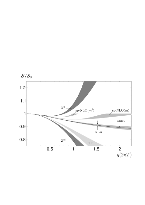
FIG. 2.: Comparison of perturbative and HTL-improved approximations to the entropy in the large-$N$ scalar O($N$)-model. The shaded areas denote the variation under changes of the renormalization scale from $\bar{\mu}^{\prime}=\pi T$ to $4\pi T$. The band marked “HTL” refers to using the leading-order (HTL) mass in the 2-loop $\Phi$-derivable entropy, “NLA” to using the approximately self-consistent NLO mass (75). Also given are the corresponding results for a naive strictly perturbative NLO mass when defined through $m^{2}$ or $m$, respectively.

In order to ensure such a monotonous behavior, in Refs. [15, 16] we have considered the simple Padé approximant $\hat{m}^{2}+\delta m^{2}\to\hat{m}^{2}/[1-\delta m^{2}/\hat{m}^{2}]=g^{2}T^{2}/[1+3g/\pi]$, which already achieves a dramatic improvement for $g\gtrsim 1$. An alternative, which is in fact more in the spirit of approximate self-consistency, is to return to the approximate gap equation (51)

$$m^{2}\,=\,g^{2}T^{2}-{3\over\pi}\,g^{2}Tm\,,$$ (74)

and solve this quadratic equation for $m$ exactly, yielding

$$m_{\rm NLA}/T=\sqrt{g^{2}+(3g^{2}/2\pi)^{2}}-3g^{2}/2\pi.$$ (75)

In what follows, this will be referred to as our “next-to-leading approximation” (NLA) for the scalar thermal mass. Also this approximation preserves the propertym of being a monotonously growing function of $g$. For very large $g$ it saturates at $m_{\mathrm{N}LA}\to(\pi/3)T$. The corresponding results for the various renormalization scale choices are given by the dotted lines in Fig. 1, showing a striking improvement over the standard perturbative results also for very large coupling.

With $m$ approximated either by its leading-order (HTL) value $\hat{m}=g(\bar{\mu})T$ or by the NLA result (74), the correspondingly approximated entropy is obtained by evaluating numerically the expression (47). In Fig. 2 this is compared with the strictly perturbative expressions for ${\cal S}/{\cal S}_{0}$ up to and including order $g^{2}$, and $g^{3}$, respectively. The shaded bands indicate the variation of the results with $\bar{\mu}^{\prime}=\pi T\ldots 4\pi T$. Evidently, the perturbative 3rd-order result fails to be a better approximation than the 2nd-order one for $g\gtrsim 1$. The semi-perturbatively evaluated HTL result is already an appreciable improvement over the 2nd-order perturbative result, whereas the NLA follows closely the exact ($N\to\infty$) result. Also shown are the results corresponding to the two “strictly perturbative” NLO mass definitions mentioned above when used in the same manner.

III QCD: Approximately self-consistent resummations

We turn now to our main case of interest, the QCD plasma. In this section, we shall concentrate on a purely gluonic plasma, deferring the addition of quarks to the next section. Although the thermodynamic potential in QCD is a gauge independent quantity, in writing down its skeleton representation we have to specify a gauge. In formulating the two-loop $\Phi$-derivable approximation we find it convenient to start with the temporal axial gauge. While this approximation is by itself gauge dependent, when supplemented by perturbative approximations on the generalized gap equation it results in a gauge invariant resummation scheme for the entropy.

A The skeleton representation of the entropy

In QCD, the thermodynamic potential is a functional of the full gluon ($D$), quark ($S$), and Faddeev-Popov ghost ($D_{gh}$) propagators,

$$\beta\Omega[D,S,D_{gh}] = {1\over 2}{\,\mathrm{T}r\,}\log D^{-1}-{\,\mathrm{T}r\,}\log S^{-1}-{\,\mathrm{T}r\,}\log D^{-1}_{gh}$$ (77)

$$-{1\over 2}{\,\mathrm{T}r\,}\Pi D+{\,\mathrm{T}r\,}\Sigma S+{\,\mathrm{T}r\,}\Pi_{gh}D_{gh}+\Phi[D,S,D_{gh}],$$

where Tr now includes traces over color indices, and also over Lorentz and spinor indices when applicable. The self-energies for gluons, quarks and ghosts are denoted respectively by $\Pi$, $\Sigma$ and $\Pi_{gh}$. In Fig. 3, the lowest-order (two-loop) skeleton diagrams for $\Phi$ are displayed.

FIG. 3.: Diagrams for $\Phi$ at 2-loop order in QCD. Wigly, plain, and dotted lines refer respectively to gluons, quarks, and ghosts.

In gauges which do not break rotational invariance, the gluon propagator at finite temperature contains up to four different structure functions [24]. Only two of them correspond to degrees of freedom which are transverse in 4 dimensions; the remaining ones are unphysical, constrained by a Ward identity [25], and compensated for by the Faddeev-Popov ghost degrees of freedom.

In general, the gluon self-energy $\Pi_{\mu\nu}(k)$ is a tensor which is not transverse with respect to the 4-momentum $k^{\mu}=(\omega,{\bf k})$, but also contains up to 4 structure functions. There are however gauges where ghosts decouple and where as a consequence $\Pi_{\mu\nu}$ is strictly transverse: axial gauges $n_{\mu}A^{a\mu}=0$, with $n_{\mu}$ a constant 4-vector.

A particularly convenient choice appears to be the temporal axial gauge, where $n_{\mu}$ coincides with the rest-frame velocity of the heat bath and thus preserves rotational invariance. Ignoring the well-known difficulties with this gauge in the imaginary-time formalism [26], the temporal axial gauge would lead to great simplifications of the structure of Eq. (77): The ghost self-energy $\Pi_{gh}$ vanishes and the ghost propagator does not appear in $\Phi$. Secondly, there are only two independent structure functions in the gluon self-energy, which can then be written as (suppressing the color labels)

$$\Pi_{ij}(\omega,k)=\left(\delta_{ij}-{k_{i}k_{j}\over k^{2}}\right)\Pi_{T}(\omega,k)-{k_{i}k_{j}\omega^{2}\over k^{4}}\Pi_{L}(\omega,k),$$ (78)

$$\Pi_{00}(\omega,k)=-\Pi_{L}(\omega,k),\qquad\Pi_{0i}(\omega,k)=-{\omega k_{i}\over k^{2}}\Pi_{L}(\omega,k).$$ (79)

With these definitions, the propagator in temporal axial gauge reads

$$D_{ij}^{\rm TAG}(\omega,k)=\left(\delta_{ij}-{k_{i}k_{j}\over k^{2}}\right)D_{T}(\omega,k)+{k_{i}k_{j}\over k^{2}}{k^{2}\over\omega^{2}}D_{L}(\omega,k)$$ (80)

where

$$D_{T}(\omega,k)\,\equiv\,\frac{-1}{\omega^{2}-k^{2}-\Pi_{T}(\omega,k)}\,,\qquad D_{L}(\omega,k)\,\equiv\,\frac{-1}{k^{2}+\Pi_{L}(\omega,k)}\,.$$ (81)

Note that because $D^{\rm TAG}_{0\mu}=D^{\rm TAG}_{\mu 0}\equiv 0$, only the spatial components $\Pi_{ij}$ of the polarization tensor enter Eq. (77) in temporal axial gauge.

For later use we introduce the following spectral representations:

$$D_{T}(\omega,k) = \int_{-\infty}^{\infty}\frac{{\rm d}k_{0}}{2\pi}\,\frac{\rho_{T}(k_{0},k)}{k_{0}-\omega}\,,$$ (82)

$$D_{L}(\omega,k) = -\,\frac{1}{k^{2}}\,+\int_{-\infty}^{\infty}\frac{{\rm d}k_{0}}{2\pi}\,\frac{\rho_{L}(k_{0},k)}{k_{0}-\omega}\,.$$ (83)

Here $\rho_{T}$ and $\rho_{L}$ are the spectral densities:

$$\rho_{L,T}(k_{0},k)\,\equiv\,\lim_{\eta\to 0}2\,{\rm Im}\,D_{L,T}(k_{0}+i\eta,k)\,.$$ (84)

[Note the subtraction performed in the spectral representation of $D_{L}(\omega,k)$: this is necessary since $D_{L}(\omega,k)\to-1/k^{2}$ as $|\omega|\to\infty$. At tree-level, $\rho_{L}^{(0)}=0$ and $\rho_{T}^{(0)}=2\pi\epsilon(k_{0})\delta(k^{2})$, and therefore $D_{T}^{(0)}=-1/(\omega^{2}-k^{2})$ and $D_{L}^{(0)}=-1/k^{2}$.]

Concentrating on the gluonic contributions for now and postponing the inclusion of fermions to the next section, we obtain in analogy to Eq. (12)

$$\Omega_{g}/V = N_{g}\int\!\!{d^{4}k\over(2\pi)^{4}}\,n(\omega)\biggl{\{}2\left({\,\mathrm{I}m\,}\log(-\omega^{2}+k^{2}+\Pi_{T})-{\,\mathrm{I}m\,}\Pi_{T}D_{T}\right)$$ (86)

$$\qquad\qquad+\left({\,\mathrm{I}m\,}\log(k^{2}+\Pi_{L})+{\,\mathrm{I}m\,}\Pi_{L}D_{L}\right)\biggr{\}}+T\Phi_{g}[D_{T},D_{L}]/V$$

where $N_{g}$ is the number of gluons ($N^{2}-1$ for SU($N$), i.e. 8 for QCD). The entropy of purely gluonic QCD can then be written in complete analogy to the derivation of Eq. (17) as

$${\cal S}={\cal S}_{T}\,+\,{\cal S}_{L}+{\cal S}^{\prime}\,$$ (87)

where

$${\cal S}_{T} = -2N_{g}\int\!\!{d^{4}k\over(2\pi)^{4}}{\partial n(\omega)\over\partial T}\Bigl{\{}{\,\mathrm{I}m\,}\log(-\omega^{2}+k^{2}+\Pi_{T})-{\,\mathrm{I}m\,}\Pi_{T}{\,\mathrm{R}e\,}D_{T}\Bigr{\}},$$ (89)

$${\cal S}_{L} = -N_{g}\int\!\!{d^{4}k\over(2\pi)^{4}}{\partial n(\omega)\over\partial T}\Bigl{\{}{\,\mathrm{I}m\,}\log(k^{2}+\Pi_{L})+{\,\mathrm{I}m\,}\Pi_{L}{\,\mathrm{R}e\,}D_{L}\Bigr{\}},$$ (90)

and

$${\cal S}^{\prime}\equiv-{\partial(T\Phi)\over\partial T}\Big{|}_{D}+N_{g}\int\!\!{d^{4}k\over(2\pi)^{4}}{\partial n(\omega)\over\partial T}\left(2{\,\mathrm{R}e\,}\Pi_{T}{\,\mathrm{I}m\,}D_{T}-{\,\mathrm{R}e\,}\Pi_{L}{\,\mathrm{I}m\,}D_{L}\right).$$ (91)

As in the scalar case, we are interested in the $\Phi$-derivable approximation obtained by keeping only the two-loop skeletons of Fig. 3. In gauge theories, however, the $\Phi$-derivable approximations have in general the drawback of violating gauge symmetry, because vertex functions are not treated on equal footing with self-energies (in particular, in the two-loop approximation to $\Phi$ there are no vertex corrections at all). Thus the corresponding approximation to the polarization tensor $\Pi_{\mu\nu}$ needs not be transverse. Nevertheless, in the temporal axial gauge, the previous expressions are not affected by a loss of 4-dimensional transversality, because they involve only the spatial components $\Pi_{ij}$, or equivalently $\Pi_{T}$ and $\Pi_{L}$ (cf. Eq. (78)).

Therefore, in this gauge, the property that ${\cal S}^{\prime}=0$ in the two-loop approximation to $\Phi$ still holds, for the same, essentially combinatorial reasons as in the scalar field theory with cubic and quartic interactions of the previous section. In this approximation, the self-energies $\Pi_{T}$, $\Pi_{L}$ and propagators $D_{T}$, $D_{L}$ are to be determined self-consistently, by solving the generalized “gap equations”

$$D^{-1}_{T}\,=\,-\omega^{2}+k^{2}+\Pi_{T}[D_{T},D_{L}]\,,\qquad D^{-1}_{L}\,=\,-\,k^{2}\,-\,\Pi_{L}[D_{T},D_{L}]\,,$$ (92)

i.e., the Dyson equations where $\Pi_{s}[D_{T},D_{L}]$ ($s=T,\,L$) are the one-loop self-energies built out of $D_{T}$ and $D_{L}$.

Whereas the entropy expressions (III A) themselves are manifestly UV finite, Eqs. (92) contain UV divergences which require renormalization. Because of the simple Ward identities of axial gauges, (wave function) renormalization of the gluon self-energy at lowest order in $g$ contains the correct one-loop coefficient of the beta function [27, 28]. Beyond lowest order, however, it is not clear that the gap equations (92) can be renormalized in a simple manner (in contrast to the scalar toy model of Sect. II B).

At any rate, in general gauges the 2-loop $\Phi$-derivable approximation misses the correct perturbative running of the coupling constant. Indeed, the latter is an order-$g^{4}$ effect in the thermodynamic potentials and is thus beyond the perturbative accuracy of a 2-loop $\Phi$-derivable approximation.

B Approximately self-consistent solutions

Unlike the scalar theory with $\lambda\phi^{4}$ interactions, in QCD the “gap equations” (92) are non-local, which makes their exact solution prohibitively difficult. But in fact, as we have just explained, uncertainties concerning gauge symmetry and renormalization beyond order $g^{3}$ make such a fully self-consistent solution not really desirable.

For this reason we shall construct approximately self-consistent solutions which maintain equivalence with conventional perturbation theory up to and including order $g^{3}$ (the maximum perturbative accuracy allowed by two-loop approximations for $\Phi$), and which are manifestly gauge-independent and UV finite. After such approximations—where the gluon polarization tensor is transverse and the ghost self-energy (in gauges with ghosts) is neglected—, Eqs. (III A) have the same formal structure in any other gauge, and ${\cal S}^{\prime}=0$ to the same accuracy. We can therefore drop the restriction to the somewhat problematic temporal axial gauge. For instance, in the more commonly used Coulomb gauge the gauge propagator is given by

$$D_{00}^{\rm CG}(\omega,k)=D_{L}(\omega,k),\quad D_{ij}^{\rm CG}(\omega,k)=\left(\delta_{ij}-{k_{i}k_{j}\over k^{2}}\right)D_{T}(\omega,k)$$ (93)

and the ghost propagator does not contribute as long as there is no nontrivial ghost self-energy; in covariant gauges under the same circumstances, the then propagating ghosts just compensate for an additional massless pole that is present in the gluon propagator.

With the gauge-independent approximations for $\Pi_{L,T}$ that we shall obtain from (HTL) perturbation theory, the effectively one-loop expressions for the entropy, Eqs. (III A), constitute a gauge-invariant approximation to the full entropy. By then computing exactly these expressions, we shall obtain a gauge-invariant result which is nonperturbative in the coupling $g$, while being equivalent to conventional resummed perturbation theory up to and including order $g^{3}$.

As generally with thermal field theories [8, 2], the perturbative solution of Eqs. (92) requires to distinguish between soft ($k\lesssim gT$) and hard ($k\sim T$) fields, which are dressed differently by thermal fluctuations. In (purely gluonic) QCD, and in the Coulomb gauge, the hard fields are always transverse, while the soft fields — which may be seen as collective excitations of the former [7, 8] — can be either longitudinal, or transverse.

Because of the limited phase-space, the leading order (LO) contribution of the soft modes to the thermodynamical functions is already of order $g^{3}$ [1], so the corresponding self-energies are needed only to leading order in $g$. These are the so-called hard thermal loops $\hat{\Pi}_{L}$ and $\hat{\Pi}_{T}$ [29, 9], which in the present formalism appear as the solutions to Eqs. (92) to LO in $g$ and for soft $(k\sim gT)$ external momenta. They read:

$$\hat{\Pi}_{L}(\omega,k) = \hat{m}_{D}^{2}\left[1-{\omega\over 2k}\log{\omega+k\over\omega-k}\right],$$ (94)

$$\hat{\Pi}_{T}(\omega,k) = \frac{1}{2}\left[\hat{m}_{D}^{2}+\,\frac{\omega^{2}-k^{2}}{k^{2}}\,\hat{\Pi}_{L}\right],$$ (95)

with the Debye mass

$$\hat{m}^{2}_{D} = -\,\frac{g^{2}N}{\pi^{2}}\int_{0}^{\infty}{\rm d}k\,k^{2}\,\frac{\partial n}{\partial k}\,=\,{g^{2}T^{2}N\over 3}\,.$$ (96)

The HTL’s (94) are manifestly UV finite: they derive from one-loop Feynman graphs, but involve only the contribution of the thermal fluctuations in the latter (as opposed to the vacuum fluctuations, which are responsible for UV divergences). The corresponding propagators are then defined via the Dyson equations (92):

$$\hat{D}_{T}^{-1}(\omega,k)\,=\,-\omega^{2}+k^{2}+\hat{\Pi}_{T}(\omega,k)\,,\qquad\hat{D}_{L}^{-1}(\omega,k)\,=\,-k^{2}-\hat{\Pi}_{L}(\omega,k)\,,$$ (97)

Note that, for $k\sim gT$, the self-energy corrections in Eqs. (94)–(97) are as important as the corresponding tree-level inverse propagators $D_{0}^{-1}\sim k^{2}\sim g^{2}T^{2}$. Thus, at soft momenta, the self-energies cannot be expanded out of the HTL-resummed propagators. The HTL spectral densities consist of quasiparticle poles at time-like momenta and Landau damping cuts for $|\omega|<k$. When $k\gg gT$, the transverse pole describes the usual single-particle excitations (hard transverse gluons), while the additional pole associated to the collective longitudinal excitation has exponentially vanishing residue [31].

For hard, transverse, fields, we need the solution $\Pi_{T}(k\sim T)$ of Eqs. (92) to leading, and next-to-leading order (NLO). This is obtained as:

$$\Pi_{T}(k\sim T)\simeq\Pi_{T}^{(2)}+\delta\Pi_{T},$$ (98)

where $\Pi_{T}^{(2)}\equiv\Pi_{T}[D_{0}]\sim g^{2}$ is the bare one-loop self-energy (i.e., the standard one-loop diagrams with tree-level propagators $D_{0}=(D_{T}^{(0)},D_{L}^{(0)})$ on the internal lines), and $\delta\Pi_{T}\sim g^{3}T^{2}$ is an effective one-loop self-energy where one of the internal lines is hard (and transverse), while the other one is soft (longitudinal or transverse) and dressed by the HTL. Thus, $\delta\Pi_{T}$ is the sum of the four diagrams depicted in Fig. 4; these are explicitly computed in App. A 3.

FIG. 4.: NLO contributions to $\delta\Pi_{T}$ at hard momentum. Thick dashed and wiggly lines with a blob represent HTL-resummed longitudinal and transverse propagators, respectively.

A priori, the one-loop self-energy involves also vacuum fluctuations, and therefore UV divergences, which call for renormalization. The UV divergences could be absorbed by a wave-function renormalization constant, which drops out from the entropy expressions (III A). As it will turn out presently, only the light-cone limit of $\Pi_{T}[D_{0}]$ will contribute to the order of interest. In line with our strategy of restricting to gauge-invariant approximations to the self-energy, we shall altogether drop the gauge-dependent vacuum pieces, which in fact vanish on the light-cone.

Because from standard HTL perturbation theory we take UV finite approximations for $\Pi_{L,T}$, we shall in fact have no inherent beta function prescribing the scale dependence of the coupling $g$. When numerically evaluating the results, we shall simply adopt the standard running coupling constant of the $\overline{\hbox{MS}}$ scheme and consider the resulting renormalization-scale dependence of our results as an estimate of our theoretical error (cf. Sect. II D).

C Perturbation theory: Lowest orders

In this and the following subsections, we shall consider the perturbative expansion of our master equation for the entropy, Eqs. (III A), and recover in the process the standard perturbative results up to order $g^{3}$. This is useful not only as a cross check of the various approximations, but also as an illustration of the rather non-trivial way that perturbation theory gets reorganized by this equation. Moreover, the perturbative expansion will shed more light on the physical interpretation of the various terms in Eqs. (III A), and give us hints for better approximations to be used in the non-perturbative, numerical calculations to come.

The leading-order result is obtained by putting $\Pi_{T}=\Pi_{L}=0$ in Eqs. (III A). This is the Stefan-Boltzmann entropy of a free gas of massless transverse gluons:

$${\cal S}_{SB} = -2N_{g}\int\!\!{d^{4}k\over(2\pi)^{4}}{\partial n(\omega)\over\partial T}\,{\,\mathrm{I}m\,}\log(-\omega^{2}+k^{2})$$ (99)

$$= -2N_{g}\int\!\!{d^{3}k\over(2\pi)^{3}}{\partial\over\partial T}\Bigl{[}T\log(1-e^{-k/T})\Bigr{]}=\frac{4\pi^{2}}{45}\,N_{g}T^{3}.$$ (100)

Here the retarded prescription ($\omega\to\omega+i\epsilon$) is implicit in the first integral, which is evaluated with the help of the identities (48) and (34).

The order-$g^{2}$ contribution to the entropy comes also exclusively from hard transverse gluons, via one-loop corrections. Specifically, by expanding Eq. (89) to order $g^{2}$, one obtains:

$${\cal S}_{2} = -2N_{g}\int\!\!{d^{4}k\over(2\pi)^{4}}\,{\partial n\over\partial T}\left\{-{\,\mathrm{I}m\,}\frac{\Pi_{T}^{(2)}}{\omega^{2}-k^{2}}+{\,\mathrm{I}m\,}{\Pi_{T}^{(2)}}{\,\mathrm{R}e\,}\frac{1}{\omega^{2}-k^{2}}\right\}$$ (101)

$$= 2N_{g}\int\!\!{d^{4}k\over(2\pi)^{4}}\,{\partial n\over\partial T}\,{\,\mathrm{R}e\,}{\Pi_{T}^{(2)}}{\,\mathrm{I}m\,}\frac{1}{\omega^{2}-k^{2}}$$ (102)

$$= -2\pi N_{g}\int\!\!{d^{4}k\over(2\pi)^{4}}\,{\partial n\over\partial T}\,\epsilon(\omega)\delta(\omega^{2}-k^{2}){\,\mathrm{R}e\,}\Pi_{T}^{(2)}(\omega,k),$$ (103)

where the integral is indeed dominated by hard momenta $k\sim T$. Note that ${\cal S}^{(2)}$ involves only the light-cone projection ${\,\mathrm{R}e\,}\Pi_{T}^{(2)}(\omega=k)$ of the one-loop self-energy for (hard) transverse gluons $\Pi_{T}^{(2)}(\omega,k)$. This projection is a priori UV finite: indeed, gauge symmetry guarantees that the vacuum contribution to ${\,\mathrm{R}e\,}\Pi_{T}^{(2)}(\omega=k)$ must vanish. Moreover, quite remarkably, this projection turns out to be also momentum-independent [32],

$$\Pi_{T}^{(2)}(\omega^{2}=k^{2})=g^{2}NT^{2}/6\equiv m_{\infty}^{2},$$ (104)

and thus defines a (thermal) mass correction, also known as the asymptotic mass. Thus, finally,

$${\cal S}_{2} = -N_{g}{m_{\infty}^{2}T\over 6}=-{NN_{g}\over 36}g^{2}T^{3},$$ (105)

which is indeed the correct result [1]. Note also that at leading order the asymptotic mass is simply related to the (HTL) Debye mass: $m_{\infty}^{2}=\hat{m}^{2}_{D}/2$.

It is worth emphasizing that Eq. (101) is the same as the entropy of an ideal gas of massive particles (with constant masses equal to $m_{\infty}$) when expanded to leading order in $m_{\infty}^{2}$. As was the case in the scalar model discussed in Sect. II, such a simple identification is specific to the entropy, and does not hold for the order-$g^{2}$ effect in the pressure.

In the scalar case we have seen that the HTL-resummed one-loop pressure over-includes the LO interaction term by a factor of two. For gluons, Ref. [11] reported instead a factor of three. Inspecting the corresponding calculation reveals that this arises because of an incomplete implementation of dimensional regularisation. While in the latter $2-2\epsilon$ transverse polarisations of the gluons are considered, the HTL expressions for $\Pi_{\mu\nu}$ have not been modified accordingly. However in $d\not=3$ spatial dimensions, Eqs. (95,94) become

$$\hat{\Pi}_{T}={1\over d-1}\left[\hat{m}_{D}^{2}+\frac{\omega^{2}-k^{2}}{k^{2}}\,\hat{\Pi}_{L}\right],\quad\hat{\Pi}_{L}=\hat{m}_{D}^{2}\left[1-\,{}_{2}F_{1}({1\over 2},1;{d\over 2};{k^{2}\over\omega^{2}})\right],$$ (106)

where

$$\hat{m}_{D}^{2}=(d-1)g^{2}NT^{2}({T\over\mu})^{d-3}{\zeta(d-1)\Gamma({d+1\over 2})\over\pi^{(d+1)/2}}\qquad(d>2)$$ (107)

as determined by the $d$-dimensional analog of Eq. (96). This gives a real and constant $\hat{\Pi}^{\mu}_{\mu}=\hat{m}_{D}^{2}=(d-1)m_{\infty}^{2}$ such that the order-$g^{2}$ contribution to the 1-loop HTL-resummed pressure $P_{HTL}=-{1\over 2}{\,\mathrm{T}r\,}\log(D_{0}^{-1}+\hat{\Pi})$ is

$$P_{HTL}^{(2)}=N_{g}\int\!\!{d^{d+1}k\over(2\pi)^{d+1}}\,n(\omega){\,\mathrm{I}m\,}\frac{\hat{\Pi}^{\mu}_{\mu}}{\omega^{2}-k^{2}}=N_{g}\hat{m}_{D}^{2}\int\!\!{d^{d+1}k\over(2\pi)^{d+1}}\,n(\omega){\,\mathrm{I}m\,}\frac{1}{\omega^{2}-k^{2}}\to 2\times P_{2}$$ (108)

as $d\to 3$, with dimensional regularization eliminating the quadratic divergence for $\omega\to-\infty$. This is then consistent with momentum cut-off regularization, where $d=3$ can be kept throughout, after dropping a divergence $\propto\hat{m}_{D}^{2}\Lambda^{2}$. Presumably, the numerical results reported in Ref. [11] will change significantly when corrected accordingly.

This sensitivity to (a consistent usage of) regularization schemes is related in fact to the UV behavior of HTL-screened perturbation theory; it is not present in our UV-finite HTL-resummation of (two-loop) entropy and density.

D Perturbation theory: Order $g^{3}$

The extraction of the order-$g^{3}$ contribution to the entropy in Eq. (III A) turns out to be more intricate than the standard calculation of the plasmon effect in the pressure [1].

1 The order $g^{3}$ in the pressure

Let us briefly discuss first the plasmon effect in the pressure, as obtained from the skeleton representation (5). As explained for the scalar case in Sect. II C, the order-$g^{3}$ contribution to the pressure comes entirely from soft momenta, and reads (cf. Eq. (64)):

$$P_{3} = -\int\!\!{d^{4}k\over(2\pi)^{4}}\,\frac{T}{\omega}\,{\,\mathrm{I}m\,}\Bigl{[}\log(1+D_{0}\hat{\Pi})-D_{0}\hat{\Pi}\Bigr{]}\,.$$ (109)

In QCD, $D=(D_{T},D_{L})$, $\hat{\Pi}=(\hat{\Pi}_{T},-\hat{\Pi}_{L})$, and a sum over color and polarization states is implicit in (109). [Note the minus sign in front of $\Pi_{L}$ in these compact notations; this reflects our conventions in Eqs. (78)–(81).] The integral over $\omega$ yields:

$$\int\frac{d\omega}{\pi\omega}\,{\,\mathrm{I}m\,}\Bigl{[}\log(1+D_{0}\hat{\Pi})-\hat{\Pi}D_{0}\Bigr{]} = \log\Bigl{[}1+D_{0}(\omega=0)\hat{\Pi}(\omega=0)\Bigr{]}-\hat{\Pi}(\omega=0)D_{0}(\omega=0)$$ (110)

$$= \log\left(1+\frac{\hat{m}_{D}^{2}}{k^{2}}\right)-\frac{\hat{m}_{D}^{2}}{k^{2}}\,,$$ (111)

where the non-vanishing contribution in the second line comes from the longitudinal sector alone [33], since $\hat{\Pi}_{L}(\omega=0)=\hat{m}_{D}^{2}$, while $\hat{\Pi}_{T}(\omega=0)=0$. Thus,

$$P_{3} = -N_{g}T\int\!\!{d^{3}k\over(2\pi)^{3}}\,\left[\log\left(1+\frac{\hat{m}_{D}^{2}}{k^{2}}\right)-\frac{\hat{m}_{D}^{2}}{k^{2}}\right]\,=\,N_{g}\frac{\hat{m}_{D}^{3}T}{12\pi},$$ (112)

where the color factor $N_{g}=N^{2}-1$ has been reintroduced. Eq. (112) is indeed the standard result for $P_{3}$, generally obtained by summing the ring diagrams in the imaginary-time perturbation theory [1].

The order-$g^{3}$ effect in the entropy can be now directly calculated as the total derivative of $P_{3}$ with respect to $T$. We thus obtain ${\cal S}_{3}={\cal S}_{3}^{(a)}+{\cal S}_{3}^{(b)}$, where

$${\cal S}_{3}^{(a)}\equiv\frac{{\partial}P_{3}}{{\partial}T}\bigg{|}_{\hat{m}_{D}}\,=\,-N_{g}\int\!\!{d^{4}k\over(2\pi)^{4}}\,{\partial n(\omega)\over\partial T}\,{\,\mathrm{I}m\,}\Bigl{[}\log(1+D_{0}\hat{\Pi})-\hat{\Pi}D_{0}\Bigr{]}\,=\,N_{g}\frac{\hat{m}_{D}^{3}}{12\pi}\,,$$ (114)

is the derivative at fixed $\Pi=\hat{\Pi}$ (recall that the HTL’s depend upon the temperature only via the Debye mass; cf. Eqs. (94) and (96)), and

$${\cal S}_{3}^{(b)}\equiv\frac{{\partial}P_{3}}{{\partial}\hat{m}_{D}}\,\frac{{\rm d}\hat{m}_{D}}{{\rm d}T}\,=\,-N_{g}\int\!\!{d^{4}k\over(2\pi)^{4}}\,n(\omega)\,{\,\mathrm{I}m\,}\left[\frac{{\rm d}\hat{\Pi}}{{\rm d}T}(\hat{D}-D_{0})\right]=\,N_{g}\frac{\hat{m}_{D}^{3}}{4\pi}\,.$$ (115)

This decomposition of ${\cal S}_{3}$ is interesting in view of the comparison with the perturbative expansion of Eqs. (III A), to which we now turn.

2 The order $g^{3}$ in the entropy

Unlike what happens for the pressure, the order-$g^{3}$ effects of the hard modes do not cancel in Eqs. (III A), similarly to what we have observed in the scalar case in Sect. II C. Rather, we get a non-zero such contribution by replacing ${\,\mathrm{R}e\,}\Pi_{T}^{(2)}\longrightarrow{\,\mathrm{R}e\,}\delta\Pi_{T}$ in Eq. (101), with $\delta\Pi_{T}\sim g^{3}T^{2}$ the NLO self-energy correction of hard transverse gluons (cf. Eq. (98)). This yields:

$${\cal S}_{3}^{\mathrm{h}ard} = -N_{g}\int\!\!{d^{3}k\over(2\pi)^{3}}\,{1\over k}\,{\partial n(k)\over\partial T}\,{\,\mathrm{R}e\,}\delta\Pi_{T}(\omega=k).$$ (116)

Once again, we need only the light-cone projection of the self-energy of the hard particles. What is, however, new as compared to the situation at order $g^{2}$ is that ${\,\mathrm{R}e\,}\delta\Pi_{T}(\omega=k)$ is not a constant “mass correction”, but rather a complicated function of $k$ (see Eqs. (A20) and (A22)). The calculation of ${\cal S}_{3}^{\mathrm{h}ard}$ is deferred to the Appendix, but the final result can be anticipated, as we shall see shortly.

The other contributions of order $g^{3}$ come from the soft gluons, which can be longitudinal or transverse, and we write ${\cal S}_{3}^{\mathrm{s}oft}={\cal S}_{L}^{(3)}+{\cal S}_{T}^{(3)}$. We have (with $n(\omega)\simeq T/\omega$):

$${\cal S}_{L}^{(3)} = -N_{g}\int\!\!{d^{4}k\over(2\pi)^{4}}\,{1\over\omega}\,\Bigl{\{}{\,\mathrm{I}m\,}\log(k^{2}+\hat{\Pi}_{L})+{\,\mathrm{I}m\,}\hat{\Pi}_{L}{\,\mathrm{R}e\,}\hat{D}_{L}\Bigr{\}},$$ (117)

$${\cal S}_{T}^{(3)} = -2N_{g}\int\!\!{d^{4}k\over(2\pi)^{4}}\,{1\over\omega}\biggl{\{}{\,\mathrm{I}m\,}\left[\log\left(1-\frac{\hat{\Pi}_{T}}{\omega^{2}-k^{2}}\right)+\frac{\hat{\Pi}_{T}}{\omega^{2}-k^{2}}\right]$$ (119)

$$\qquad\qquad\qquad\qquad-{\,\mathrm{I}m\,}\hat{\Pi}_{T}{\,\mathrm{R}e\,}\Bigl{(}\hat{D}_{T}-D_{T}^{(0)}\Bigr{)}\biggr{\}},$$

where in the transverse sector, the contribution of order $g^{2}$ has been subtracted (cf. Eq. (101)). More precisely, Eq. (101) involves the full one-loop self-energy $\Pi_{T}^{(2)}$, while the subtracted terms in Eq. (119) involve only $\hat{\Pi}_{T}$, the HTL. This is nevertheless correct since $\Pi_{T}^{(2)}$ and $\hat{\Pi}_{T}$ coincide on the light-cone:

$$\hat{\Pi}_{T}(\omega^{2}=k^{2})=\Pi_{T}^{(2)}(\omega^{2}=k^{2})=m_{\infty}^{2}.$$ (120)

Ultimately, all the contributions of order $g^{3}$ displayed in Eqs. (116)–(119) are soft field effects: the quantities ${\cal S}_{L}^{(3)}$ and ${\cal S}_{T}^{(3)}$ are the LO entropies of the soft gluons, while ${\cal S}_{3}^{\mathrm{h}ard}$ is the NLO correction to the entropy of the hard gluons induced by their coupling to the soft fields (cf. Fig. 4). We expect these three contributions to add to the standard result for the plasmon effect in the entropy, namely (cf. Eqs. (III D 1)):

$${\cal S}_{3}^{\mathrm{s}oft}+{\cal S}_{3}^{\mathrm{h}ard}\,=\,{\cal S}_{3}\,\equiv\,N_{g}\hat{m}_{D}^{3}/(3\pi).$$ (121)

This is verified in the Appendix, where the quantities in Eqs. (116)–(119) are explicitly computed, but it can be also understood on the basis of the following argument.

Eqs. (116)–(119) can be compactly rewritten as

$${\cal S}_{3} = -\int\!\!{d^{4}k\over(2\pi)^{4}}\,\frac{1}{\omega}\left\{{\,\mathrm{I}m\,}\Bigl{[}\log(1+D_{0}\hat{\Pi})-\hat{\Pi}D_{0}\Bigr{]}\,-\,{\,\mathrm{I}m\,}\hat{\Pi}{\,\mathrm{R}e\,}(\hat{D}-D_{0})\right\}-$$ (123)

$$\,\,\,\,-\,\int\!\!{d^{4}p\over(2\pi)^{4}}{\partial n(p_{0})\over\partial T}{\,\mathrm{R}e\,}\delta\Pi{\,\mathrm{I}m\,}D_{0}\,,$$

where the sum over color and polarization states is again implicit. The first term within the (soft) integral over $k$ is obviously the same as ${\cal S}_{3}^{(a)}$, the temperature derivative of $P_{3}$ at fixed $\hat{m}_{D}$ (cf. Eq. (114)). It thus remains to show that the other terms in Eq. (123) add to ${\cal S}_{3}^{(b)}$, the piece of the entropy involving the derivative of the Debye mass (cf. Eq. (115)). That is, one has to prove the following relation:

$$\int\!\!{d^{4}p\over(2\pi)^{4}}{\partial n(p_{0})\over\partial T}{\,\mathrm{R}e\,}\delta\Pi{\,\mathrm{I}m\,}D_{0}=\int\!\!{d^{4}k\over(2\pi)^{4}}\biggl{\{}{\partial n(\omega)\over\partial T}{\,\mathrm{I}m\,}\hat{\Pi}{\,\mathrm{R}e\,}(\hat{D}-D_{0})$$ (124)

$$\qquad\,\,\,\,+n(\omega){\,\mathrm{I}m\,}\biggl{[}\frac{{\rm d}\hat{\Pi}}{{\rm d}T}(\hat{D}-D_{0})\biggr{]}\biggr{\}}.$$ (125)

Eq. (124) is nothing but the general 2-loop identity ${\cal S}^{\prime}=0$ expanded to the order $g^{3}$. Indeed, to order $g^{3}$, Eq. (18) implies:

$${\partial(T\Phi_{3})\over\partial T}\Big{|}_{D}=\int\!\!{d^{4}k\over(2\pi)^{4}}{\partial n(\omega)\over\partial T}{\,\mathrm{R}e\,}\hat{\Pi}{\,\mathrm{I}m\,}(\hat{D}-D_{0})+\int\!\!{d^{4}p\over(2\pi)^{4}}{\partial n(p_{0})\over\partial T}{\,\mathrm{R}e\,}\delta\Pi{\,\mathrm{I}m\,}D_{0},$$ (126)

where the first integral is saturated by soft momenta $k\sim gT$, while the second one is dominated by $p$ hard, $p\sim T$. On the other hand, $\Phi_{3}[D]$ has the explicit expression

$$T\Phi_{3}[D]\,\equiv\,{T\over 2}{\,\mathrm{T}r\,}[\Pi[D_{0}]\,(D-D_{0})]\,\simeq\,\int\!\!{d^{4}k\over(2\pi)^{4}}\,n(\omega)\,{\,\mathrm{I}m\,}[\hat{\Pi}\,(\hat{D}-D_{0})]$$ (127)

which implies:

$${\partial(T\Phi_{3})\over\partial T}\Big{|}_{D}=\int\!\!{d^{4}k\over(2\pi)^{4}}\left\{{\partial n(\omega)\over\partial T}{\,\mathrm{I}m\,}[\hat{\Pi}(\hat{D}-D_{0})]+n(\omega){\,\mathrm{I}m\,}\biggl{[}\frac{{\rm d}\hat{\Pi}}{{\rm d}T}(\hat{D}-D_{0})\biggr{]}\right\}.$$ (128)

A comparison of Eqs. (126) and (128) immediately leads to Eq. (124).

Moreover, the soft longitudinal and transverse sectors are decoupled at this order: $\Phi_{3}[D]$ in Eq. (127) is simply the sum of two two-loop diagrams, one with a soft electric gluon, the other one with a soft magnetic gluon. The condition ${\cal S}^{\prime}=0$ can be applied to any of these two diagrams separately. It follows that Eq. (124) must hold separately in the electric, and the magnetic sector. This is explicitly verified in the Appendix, via a lengthy calculation. Remarkably, Eq. (124) provides a relation between the effects of thermal fluctuations on the hard and soft excitations, which are both encoded in the two-loop diagrams for $\Phi_{3}$: By opening up the soft line in $\Phi_{3}$, one obtains the hard one-loop diagram responsible for the HTL $\hat{\Pi}$; by opening up one of the hard lines, one gets the effective one-loop diagrams for $\delta\Pi$ displayed in Fig. 4. In the case of the scalar theory, this relation is explicitly verified in Eqs. (68)–(70).

Let us conclude this subsection on perturbation theory with a comment on the higher-order contributions to ${\cal S}_{L}\,$: By inspection of Eq. (90), it is easy to verify that not only the LO contribution $\sim g^{3}$ discussed above, but also the corrections of order $g^{4}$ and $g^{5}$, come exclusively from soft momenta. Indeed, one can estimate the contribution of hard momenta by expanding the integrand in Eq. (90) in powers of $\Pi_{L}/k^{2}$, to obtain:

$${\,\mathrm{I}m\,}\log(k^{2}+\Pi_{L}) = {{\,\mathrm{I}m\,}\Pi_{L}\over k^{2}}-{1\over 2}{{\,\mathrm{I}m\,}(\Pi_{L})^{2}\over k^{4}}+\,\cdots\,=\,{{\,\mathrm{I}m\,}\Pi_{L}\over k^{2}}-{{\,\mathrm{I}m\,}\Pi_{L}{\,\mathrm{R}e\,}\Pi_{L}\over k^{4}}+\,\cdots$$ (129)

$$-{\,\mathrm{I}m\,}\Pi_{L}{\,\mathrm{R}e\,}{1\over k^{2}+\Pi_{L}} = -{{\,\mathrm{I}m\,}\Pi_{L}\over k^{2}}+{{\,\mathrm{I}m\,}\Pi_{L}{\,\mathrm{R}e\,}\Pi_{L}\over k^{4}}+\,\cdots\,,$$ (130)

up to terms of order $(\Pi_{L}/k^{2})^{3}$. Remarkably, not only the LO terms, but also the NLO ones, of order $g^{4}$, mutually cancel in the sum of the above equations. Thus, as anticipated, the hard modes contribute to ${\cal S}_{L}$ only at order $g^{6}$ or higher. This shows that our approximation scheme is rather insensitive to the unphysical, hard longitudinal modes. This is to be contrasted to the direct HTL resummation of the pressure where, to one-loop order, the longitudinal sector is sensitive to hard momenta already at order $g^{4}$, as indicated by the presence of UV divergences at this order [11].

3 The HTL entropy

Since $\delta\Pi_{T}(\omega=k)$ is a complicated, non-local function, whose numerical treatment is difficult, it is interesting to explore first approximations where $\delta\Pi_{T}$ is set to zero. Specifically, let us define the following approximation to the entropy, which is obtained from Eqs. (III A) by replacing all propagators and self-energies by their HTL counterparts:

$${\cal S}_{HTL} = -N_{g}\int\!\!{d^{4}k\over(2\pi)^{4}}{\partial n(\omega)\over\partial T}\,\,\Bigl{\{}2{\,\mathrm{I}m\,}\log(-\omega^{2}+k^{2}+\hat{\Pi}_{T})$$ (132)

$$\qquad\quad-2{\,\mathrm{I}m\,}\hat{\Pi}_{T}{\,\mathrm{R}e\,}\hat{D}_{T}+{\,\mathrm{I}m\,}\log(k^{2}+\hat{\Pi}_{L})+{\,\mathrm{I}m\,}\hat{\Pi}_{L}{\,\mathrm{R}e\,}\hat{D}_{L}\Bigr{\}}.$$

We shall succinctly refer to this as the HTL entropy. Clearly, this is still a non-perturbative approximation, since its expansion contains all orders in $g$.

A priori, Eq. (132) is not doing justice to the hard particles, since it uses the HTL corrections for both hard and soft momenta (while we know that the HTL’s are the LO self-energies for soft momenta alone). But it turns out that the order-$g^{2}$ effect, which is entirely due to the hard fields, is nevertheless correctly reproduced by Eq. (132): ${\cal S}_{HTL}^{(2)}={\cal S}_{2}$. The point, as emphasized in Sect. III C, is that ${\cal S}_{2}$ is sensitive only to the light-cone projection of the self-energy, where the HTL $\hat{\Pi}_{T}$ is a good LO approximation for the hard modes (cf. Eq. (120)).

On the other hand, ${\cal S}_{HTL}$ contains only a part of the $g^{3}$ effect, namely that part which is associated with the entropy of soft gluons: indeed, it is obvious that the order-$g^{3}$ contribution to Eq. (132) comes from soft momenta alone, where it coincides with ${\cal S}_{3}^{\mathrm{s}oft}={\cal S}_{L}^{(3)}+{\cal S}_{T}^{(3)}$, cf. Eqs. (117)–(119). Let us therefore study this quantity in more detail (it is the same as the first integral in Eq. (123)):

$${\cal S}_{HTL}^{(3)} = -\int\!\!{d^{4}k\over(2\pi)^{4}}\,\frac{1}{\omega}\left\{{\,\mathrm{I}m\,}\Bigl{[}\log(1+D_{0}\hat{\Pi})-\hat{\Pi}D_{0}\Bigr{]}\,-\,{\,\mathrm{I}m\,}\hat{\Pi}{\,\mathrm{R}e\,}(\hat{D}-D_{0})\right\}$$ (133)

$$= {\cal S}_{3}^{(a)}+\Delta{\cal S}_{3},$$ (134)

where ${\cal S}_{3}^{(a)}=({\partial}P_{3}/\partial T)|_{\hat{m}_{D}}={\cal S}_{3}/4$ (cf. Eq. (114)), and the remainder is

$$\Delta{\cal S}_{3} \equiv N_{g}\int\!\!{d^{4}k\over(2\pi)^{4}}\,{1\over\omega}\,\left\{2{\,\mathrm{I}m\,}\hat{\Pi}_{T}{\,\mathrm{R}e\,}\Bigl{(}\hat{D}_{T}-D_{T}^{(0)}\Bigr{)}-{\,\mathrm{I}m\,}\hat{\Pi}_{L}{\,\mathrm{R}e\,}\Bigl{(}\hat{D}_{L}-D_{L}^{(0)}\Bigr{)}\right\}$$ (135)

$$\equiv \Delta{\cal S}_{T}^{(3)}+\Delta{\cal S}_{L}^{(3)}\,.$$ (136)

Remarkably, we have found that the transverse and longitudinal contributions to $\Delta{\cal S}_{3}$ cancel within the accuracy that we have reached in a numerical integration of Eq. (135) (more than 8 significant digits). With $\Delta{\cal S}_{3}=0$, ${\cal S}_{HTL}^{(3)}$ is precisely equal to one fourth of the total $g^{3}$ effect, as it was also the case in the scalar theory with $g^{2}\phi^{4}$ self-interactions (cf. Sect. II C):

$${\cal S}_{HTL}^{(3)}\equiv{\cal S}_{T}^{(3)}+{\cal S}_{L}^{(3)}=\,\frac{{\partial}P_{3}}{{\partial}T}\bigg{|}_{\hat{m}_{D}}\,={\cal S}_{3}/4.$$ (138)

In QCD, however, this property is much more subtle: In the scalar theory, the quantity which we call here $\Delta{\cal S}_{3}$ was trivially zero, since ${\,\mathrm{I}m\,}\hat{\Pi}=0$ in that case. Here, $\Delta{\cal S}_{3}=0$ only because a compensation takes place in between the transverse and longitudinal contributions to Eq. (135), both of which arise from Landau-damping contributions at space-like momenta. Moreover, this cancellation occurs only after integrating over all energies and momenta (for generic $k$, the result of the energy integral in Eq. (135) is non-zero, see Fig. 5). Numerically, the contributions to ${\cal S}_{HTL}^{(3)}\equiv{\cal S}_{T}^{(3)}+{\cal S}_{L}^{(3)}$ turn out to be

$${\cal S}_{T}^{(3)}+{\cal S}_{L}^{(3)}=(0.34008738\ldots-0.09008738\ldots){\cal S}_{3}.$$ (139)

FIG. 5.: The integrand of Eq. (135) after performing the energy integral. The transverse $(T)$ and longitudinal $(L)$ contributions do not cancel for each value of $k$; their sum (full line) vanishes only upon integration over all $k$.

Let us summarize here the various cancellations which take place at order $g^{3}$ in the complete two-loop entropy: The straightforward perturbative expansion of our master equations (III A) leads us to Eqs. (116)–(119), and thus to the following expression for ${\cal S}_{3}$ [recall the compact notation introduced after Eq. (109)]:

$${\cal S}_{3} = {\cal S}_{3}^{\mathrm{s}oft}\,+\,{\cal S}_{3}^{\mathrm{h}ard}\,,$$ (140)

$${\cal S}_{3}^{\mathrm{s}oft} = \frac{{\partial}P_{3}}{{\partial}T}\bigg{|}_{\hat{m}_{D}}\,+\,\Delta{\cal S}_{L}^{(3)}+\Delta{\cal S}_{T}^{(3)}\,,$$ (141)

$${\cal S}_{3}^{\mathrm{h}ard} = \frac{{\partial}P_{3}}{{\partial}\hat{m}_{D}}\,\frac{{\rm d}\hat{m}_{D}}{{\rm d}T}\,-\,N_{g}\int\!\!{d^{4}k\over(2\pi)^{4}}\,{\partial n(\omega)\over\partial T}{\,\mathrm{I}m\,}\hat{\Pi}{\,\mathrm{R}e\,}(\hat{D}-D_{0})$$ (142)

$$= \frac{{\partial}P_{3}}{{\partial}\hat{m}_{D}}\,\frac{{\rm d}\hat{m}_{D}}{{\rm d}T}\,-\Delta{\cal S}_{L}^{(3)}-\Delta{\cal S}_{T}^{(3)}\,.$$ (143)

In these equations, $\Delta{\cal S}_{L}^{(3)}$ and $\Delta{\cal S}_{T}^{(3)}$ have been defined in Eq. (135), and the second line in the above expression for ${\cal S}_{3}^{\mathrm{h}ard}$ follows either by using ${\cal S}^{\prime}=0$ (cf. Sect. III.D.2), or by explicitly computing Eq. (116) within HTL-resummed perturbation theory (cf. the Appendix; see especially Eqs. (A33) and (A35) there). Furthermore, by construction, ${\cal S}_{HTL}^{(3)}$ is the same as ${\cal S}_{3}^{\mathrm{s}oft}$.

According to these equations, the quantities $\Delta{\cal S}_{L}^{(3)}$ and $\Delta{\cal S}_{T}^{(3)}$ cancel in ${\cal S}_{3}^{\mathrm{s}oft}\,+\,{\cal S}_{3}^{\mathrm{h}ard}$ independently in the longitudinal and transverse sectors, thus yielding the correct result for ${\cal S}_{3}$, cf. Eqs. (114) and (115). This is what we have been able to prove analytically (cf. Sect. III.D.2 and the Appendix). On the other hand, we have found numerically that $\Delta{\cal S}_{3}=\Delta{\cal S}_{L}^{(3)}+\Delta{\cal S}_{T}^{(3)}=0$, so that the actual results for ${\cal S}_{3}^{\mathrm{s}oft}$ and ${\cal S}_{3}^{\mathrm{h}ard}$ are even simpler:

$${\cal S}_{3}^{\mathrm{s}oft}\,=\,\frac{{\partial}P_{3}}{{\partial}T}\bigg{|}_{\hat{m}_{D}}\,,\qquad{\cal S}_{3}^{\mathrm{h}ard}\,=\,\frac{{\partial}P_{3}}{{\partial}\hat{m}_{D}}\,\frac{{\rm d}\hat{m}_{D}}{{\rm d}T}\,.$$ (144)

At this stage, we have no fundamental understanding of the “sum rule” $\Delta{\cal S}_{3}=0$. But this serendipitous result will have important consequences in practice, as we shall see below, because it determines the magnitude of ${\cal S}_{3}^{\mathrm{h}ard}$ to be $3/4$ of ${\cal S}_{3}$, as was the case in the simple scalar model of Sect. II C, while being an incomparably more complicated expression than (70).

A full numerical evaluation of the HTL entropy, non-perturbative in $g$, will be presented in Sect. V A below, and estimates of the effects of including $\delta\Pi_{T}\sim g^{3}T^{2}$ in Sect. V B.

IV QCD: Adding the fermions

It is now straightforward to add fermions to our theory. We consider $N_{f}$ flavors of massless fermions with equal chemical potential $\mu$; we choose $\mu\geq 0$, which corresponds to an excess of fermions over antifermions for all flavors. Adding the fermions will have two effects: first, this will modify the parameters of the gluonic sector, namely the Debye mass $\hat{m}_{D}^{2}$, and therefore also the asymptotic mass $m_{\infty}^{2}=\hat{m}^{2}_{D}/2$; second, there will be new contributions to the entropy. In addition, at finite $\mu$, there is a new thermodynamic function of interest, namely the density ${\cal N}$, which shares many of the interesting properties found for $\cal S$.

The full (leading-order) Debye mass in the QGP reads [7] :

$$\hat{m}^{2}_{D} = -\,\frac{g^{2}}{2\pi^{2}}\int_{0}^{\infty}{\rm d}k\,k^{2}\,\left\{2N\,\frac{\partial n}{\partial k}\,+\,N_{f}\left(\frac{\partial f_{+}}{\partial k}\,+\,\frac{\partial f_{-}}{\partial k}\right)\right\}$$ (145)

$$= (2N+N_{f})\,\frac{g^{2}T^{2}}{6}\,+\,N_{f}\,{g^{2}\mu^{2}\over 2\pi^{2}}\,.$$ (146)

We have introduced here the statistical distribution functions for fermions ($f_{+}$) and antifermions ($f_{-}$),

$$f_{\pm}(k)\,\equiv\,\frac{1}{{\rm e}^{\beta(k\mp\mu)}+1}\,,$$ (147)

and we have used the following integral:

$$\int{\rm d}k\,k\Bigl{(}f_{+}(k)+f_{-}(k)\Bigr{)}\,=\,{\pi^{2}T^{2}\over 6}+{\mu^{2}\over 2}\,.$$ (148)

A Entropy and density from the skeleton expansion

To construct the fermion contribution to the entropy, let us return to the full skeleton representation of the thermodynamic potential (in a ghost-free gauge) and add fermions to it. This becomes

$$\beta\Omega[D,S]\,=\,{1\over 2}{\,\mathrm{T}r\,}\log D^{-1}-{1\over 2}{\,\mathrm{T}r\,}\Pi D-{\,\mathrm{T}r\,}\log S^{-1}+{\,\mathrm{T}r\,}\Sigma S+\Phi[D,S],$$ (149)

where $S$ and $\Sigma$ denote respectively the fermion propagator and self-energy, and the sum over the gluon polarization states (two transverse and one longitudinal) is implicit. $\Phi[D,S]$ is the sum of the 2-particle-irreducible “skeleton” diagrams constructed out of the propagators $D$ and $S$. Below, we shall be mainly interested in the 2-loop approximation to $\Phi[D,S]$, where the only new diagram is the one represented in Fig. 3d. The self-energies $\Sigma$ and $\Pi$ in Eq. (149) are themselves functionals of the propagators, defined as

$$\Sigma\,\equiv\,{\delta\Phi[D,S]\over\delta S},\qquad\Pi\,\equiv\,2\,{\delta\Phi[D,S]\over\delta D}\,.$$ (150)

The self-consistent propagators $D$ and $S$ are obtained by solving the Dyson equations

$$D^{-1}\,=\,D^{-1}_{0}+\Pi,\qquad S^{-1}\,=\,S^{-1}_{0}+\Sigma.$$ (151)

Then, the functional $\Phi[D,S]$ is stationary under variations of $D$ and $S$ around the solutions to Eqs. (151):

$${\delta\Omega[D,S]/\delta S}=0,\qquad{\delta\Omega[D,S]/\delta D}=0.$$ (152)

The entropy ${\cal S}(T,\mu)$ and the density ${\cal N}(T,\mu)$ are obtained as the derivatives of the thermodynamic potential with respect to the temperature, and the chemical potential, respectively:

$${\cal S}\,=\,-\,\frac{\partial({\Omega/V})}{\partial T}\Big{|}_{\mu}\,,\qquad{\cal N}\,=\,-\,\frac{\partial({\Omega/V})}{\partial\mu}\Big{|}_{T}\,.$$ (153)

Because of the stationarity property (152), we can ignore the $T$ and $\mu$ dependences of the spectral densities of the propagators when differentiating $\Phi[D,S]$. That is, we have to differentiate only the statistical factors $n(\omega)=1/({\rm e}^{\beta\omega}-1)$ and $f(\omega)=1/({\rm e}^{\beta(\omega-\mu)}+1)$ which arise after performing the Matsubara sums in Eq. (149). This yields, for the entropy,

$${\cal S}\,=\,-\,\frac{\partial({\Omega/V})}{\partial T}\Big{|}_{\mu,D,S}\,\equiv\,{\cal S}_{b}+{\cal S}_{f}+{\cal S}^{\prime},$$ (154)

where ${\cal S}_{b}={\cal S}_{T}+{\cal S}_{L}$ is the purely gluonic part of the entropy, as shown in Eqs. (87)–(90), ${\cal S}_{f}$ is the corresponding fermionic piece, which reads (the trace below refers to Dirac indices)

$${\cal S}_{f} \equiv -2\int\!\!{d^{4}k\over(2\pi)^{4}}{\partial f(\omega)\over\partial T}\,{\,\mathrm{t}r\,}\left\{{\,\mathrm{I}m\,}\log(\gamma_{0}S^{-1})\,-\,{\,\mathrm{I}m\,}(\gamma_{0}\Sigma){\,\mathrm{R}e\,}(S\gamma_{0})\right\},$$ (155)

and

$${\cal S}^{\prime}\equiv-{\partial(T\Phi)\over\partial T}\Big{|}_{D,S}+\int\!\!{d^{4}k\over(2\pi)^{4}}\left\{{\partial n(\omega)\over\partial T}{\,\mathrm{R}e\,}\Pi{\,\mathrm{I}m\,}D+2{\partial f(\omega)\over\partial T}{\,\mathrm{t}r\,}\Bigl{[}{\,\mathrm{R}e\,}(\gamma_{0}\Sigma){\,\mathrm{I}m\,}(S\gamma_{0})\Bigr{]}\right\}$$ (156)

has the important property to vanish at 2-loop order [20]. That is, ${\cal S}\simeq{\cal S}_{b}+{\cal S}_{f}$ to the order of interest.

The corresponding expression for the density is obtained by replacing $(\partial f/\partial T)\to(\partial f/\partial\mu)$ in all the formulae above. This gives ${\cal N}={\cal N}_{f}+{\cal N}^{\prime}$, with ${\cal N}^{\prime}=0$ in the 2-loop approximation. Thus, to the order of interest,

$${\cal N} \simeq -2\int\!\!{d^{4}k\over(2\pi)^{4}}{\partial f(\omega)\over\partial\mu}\,{\,\mathrm{t}r\,}\left\{{\,\mathrm{I}m\,}\log(\gamma_{0}S^{-1})\,-\,{\,\mathrm{I}m\,}(\gamma_{0}\Sigma){\,\mathrm{R}e\,}(S\gamma_{0})\right\}.$$ (157)

For simplicity, all the previous formulae have been written for only one fermionic degree of freedom; the corresponding formulae for $N$ colors and $N_{f}$ flavors can be obtained by multiplying the fermionic contributions above by $NN_{f}$.

Note finally the following Maxwell relations,

$$\frac{\partial{\cal S}}{\partial\mu}\Big{|}_{T}\,=\,\frac{\partial{\cal N}}{\partial T}\Big{|}_{\mu}\,,$$ (158)

which express the equality of the mixed, second order derivatives of the thermodynamic potential. In our subsequent, self-consistent construction of ${\cal S}$ and ${\cal N}$, these relations will be satisfied at the same order as the requirement of self-consistency.

B The structure of the fermion propagator

In the previous formulae we have always associated a factor of $\gamma_{0}$ with the fermion propagator and self-energy. This was possible since $\gamma_{0}^{2}=1$ and det$\,\gamma_{0}=1$; it is also convenient since, e.g., $S^{\dagger}=\gamma_{0}S\gamma_{0}$, and it is preferable to work with hermitian Dirac matrices.

In order to compute the Dirac traces in Eqs. (155)–(157), it is useful to recall the structure of the fermion propagator at finite temperature and density: The most general form of the self-energy $\Sigma$ which is compatible with the rotational and chiral symmetries is:

$$\Sigma(\omega,{\bf k})\,=\,a(\omega,k)\,\gamma^{0}\,+\,b(\omega,k){\hat{\bf k}}\cdot{\mbox{\boldmath$\gamma$}}.$$ (159)

(For a massive fermion, this would also include a mass correction, i.e., $\Sigma=a(\omega,k)\gamma^{0}+b(\omega,k){\hat{\bf k}}\cdot{\mbox{\boldmath$\gamma$}}+c(\omega,k)$.) This can be rewritten as:

$$\gamma_{0}\Sigma(\omega,{\bf k})\,=\,\Sigma_{+}(\omega,k)\Lambda_{+}(\hat{\bf k})\,-\,\Sigma_{-}(\omega,k)\Lambda_{-}(\hat{\bf k}),$$ (160)

where $\Sigma_{\pm}(\omega,k)\equiv b(\omega,k)\pm\,a(\omega,k)$, and the spin matrices

$$\Lambda_{\pm}(\hat{\bf k}) \equiv \frac{1\pm\gamma^{0}\mbox{\boldmath$\gamma$}\cdot\hat{\bf k}}{2},\qquad\Lambda_{+}+\Lambda_{-}=1,$$ (161)

$$\Lambda_{\pm}^{2} = \Lambda_{\pm},\qquad\Lambda_{+}\Lambda_{-}\,=\,\Lambda_{-}\Lambda_{+}=0,\qquad{\,\mathrm{t}r\,}\Lambda_{\pm}=2,$$ (162)

project onto spinors whose chirality is equal ($\Lambda_{+}$), or opposite ($\Lambda_{-}$), to their helicity. Dyson’s equation $S^{-1}=-{\not\!k}+\Sigma$ then implies:

$$\gamma_{0}S^{-1}(\omega,{\bf k})\,=\,\Delta_{+}^{-1}(\omega,k)\Lambda_{+}\,+\,\Delta_{-}^{-1}(\omega,k)\Lambda_{-},$$ (163)

with $\Delta_{\pm}^{-1}\equiv-[\omega\mp(k+\Sigma_{\pm})]$. This is trivially inverted to yield the fermion propagator:

$$S\gamma_{0}(\omega,{\bf k})\,=\,\Delta_{+}(\omega,k)\Lambda_{+}+\Delta_{-}(\omega,k)\Lambda_{-}.$$ (164)

The presence of the projection operators $\Lambda_{\pm}$ in Eqs. (160), (163) and (164) allows one to easily compute the Dirac traces in Eqs. (155) and (157), and thus obtain:

$${\cal S}_{f} = -4\int\!\!{d^{4}k\over(2\pi)^{4}}{\partial f(\omega)\over\partial T}\,\Bigl{\{}{\,\mathrm{I}m\,}\log\Delta_{+}^{-1}\,+\,{\,\mathrm{I}m\,}\log(-\Delta_{-}^{-1})\,+$$ (166)

$$\qquad\qquad\,-\,{\,\mathrm{I}m\,}\Sigma_{+}{\,\mathrm{R}e\,}\Delta_{+}\,+\,{\,\mathrm{I}m\,}\Sigma_{-}{\,\mathrm{R}e\,}\Delta_{-}\Big{\}}.$$

The corresponding expression for ${\cal N}$ is obtained by replacing $(\partial f/\partial T)\to(\partial f/\partial\mu)$ in the equation above.

C Perturbation theory for $S_{f}\,$: order $g^{2}$

Eq. (166) will be now supplied with certain approximations for the quark self-energies $\Sigma_{\pm}$. As before, we aim at reproducing the results of perturbation theory up to order $g^{3}$. This will be achieved by approximations analogous to those employed for the gluons, namely the HTL approximation $\hat{\Sigma}_{\pm}$, supplemented by the NLO correction $\delta\Sigma_{\pm}$ to the hard fermion self-energy on the light cone.

Note, however, an important difference with respect to the gluon case: unlike the soft gluons, which contribute to the entropy already at order $g^{3}$, the soft fermions contribute only at order $g^{4}$ or higher, because their contribution is not enhanced by the statistics. Nevertheless, in our numerical calculation below, we shall carefully include the contribution of the soft fermions, appropriately dressed by the HTL. This is in line with our general strategy of constructing non-perturbative approximations for the entropy (or other thermodynamic quantities) which include as much as possible the dominant collective effects in the plasma.

In the HTL approximation, the fermion self-energies read as follows [30, 2] :

$$\hat{\Sigma}_{\pm}(\omega,k)\,=\,{\hat{M}^{2}\over k}\,\left(1\,-\,\frac{\omega\mp k}{2k}\,\log\,\frac{\omega+k}{\omega-k}\right),$$ (167)

where $\hat{M}^{2}$ is the plasma frequency for fermions, i.e., the frequency of long-wavelength ($k\to 0$) fermionic excitations ($C_{f}=(N^{2}-1)/2N$):

$$\hat{M}^{2}\,=\,\frac{g^{2}C_{f}}{4\pi^{2}}\int_{0}^{\infty}{\rm d}k\,k\Bigl{(}2n(k)+f_{+}(k)+f_{-}(k)\Bigr{)}\,=\,{g^{2}C_{f}\over 8}\left(T^{2}+{\mu^{2}\over\pi^{2}}\right).$$ (168)

We are now in position to evaluate the fermionic entropy and density up to order $g^{2}$: To zeroth order, i.e., for an ideal gas of massless fermions at temperature $T$ and chemical potential $\mu$, we obtain the well known results [1] (the color-flavor factor $NN_{f}$ is here reintroduced):

$${\cal S}_{f}^{(0)}\,=\,NN_{f}\left(\frac{7\pi^{2}T^{3}}{45}\,+\,\frac{\mu^{2}T}{3}\right),\qquad{\cal N}^{(0)}\,=\,NN_{f}\,{\mu\over 3}\left(T^{2}+{\mu^{2}\over\pi^{2}}\right).$$ (169)

The correction of order $g^{2}$ involves the fermion self-energies to one loop order, $\Sigma_{\pm}^{(2)}$ :

$${\cal S}_{f}^{(2)}/NN_{f} = -4\int\!\!{d^{4}k\over(2\pi)^{4}}\,{\partial f\over\partial T}\,\Bigl{\{}{\,\mathrm{R}e\,}\Sigma_{+}^{(2)}{\,\mathrm{I}m\,}\frac{-1}{\omega-k}\,-\,{\,\mathrm{R}e\,}\Sigma_{-}^{(2)}{\,\mathrm{I}m\,}\frac{-1}{\omega+k}\Bigr{\}}$$ (170)

$$= -2\int\!\!{d^{3}k\over(2\pi)^{3}}\,\left\{{\partial f(k)\over\partial T}{\,\mathrm{R}e\,}\Sigma_{+}^{(2)}(\omega=k)\,-\,{\partial f(-k)\over\partial T}\ {\,\mathrm{R}e\,}\Sigma_{-}^{(2)}(\omega=-k)\right\}.$$ (171)

As in the gluon case (cf. Eq. (101)), the correction of order $g^{2}$ is sensitive only to the light-cone projection of the one-loop self-energy, which is correctly reproduced by the HTL approximation (167) [32]. That is,

$${\,\mathrm{R}e\,}\Sigma_{\pm}^{(2)}(\omega=\pm k)\,=\,\hat{\Sigma}_{\pm}(\omega=\pm k)\,=\,{\hat{M}^{2}\over k}\,.$$ (172)

Eqs. (164) and (172) show that, to order $g^{2}$, the hard fermions (or antifermions) propagate as massive particles, with dispersion relation $\varepsilon_{k}^{2}=k^{2}+2\hat{M}^{2}$. This identifies the fermionic asymptotic mass as $M^{2}_{\infty}=2\hat{M}^{2}$. By also using the properties $f(k)=f_{+}(k)$ and $f(-k)=1-f_{-}(k)$ (cf. Eq. (147)), together with Eq. (148), we finally deduce

$${\cal S}_{f}^{(2)}/NN_{f}\,=\,-\,{\hat{M}^{2}\over\pi^{2}}\,{\partial\over\partial T}\,\left[{\pi^{2}T^{2}\over 6}+{\mu^{2}\over 2}\right]\,=\,-\,{\hat{M}^{2}T\over 3}\,=\,-\,{M^{2}_{\infty}T\over 6}\,.$$ (173)

The leading-order correction to the density ${\cal N}_{f}^{(2)}$ is obtained similarly:

$${\cal N}^{(2)}_{f}/NN_{f}\,=\,-\,{\hat{M}^{2}\over\pi^{2}}\,{\partial\over\partial\mu}\,\left[{\pi^{2}T^{2}\over 6}+{\mu^{2}\over 2}\right]\,=\,-\,{\mu\hat{M}^{2}\over\pi^{2}}\,=\,-\,{\mu M^{2}_{\infty}\over 2\pi^{2}}\,.$$ (174)

The above results for ${\cal S}_{f}^{(2)}$ and ${\cal N}^{(2)}_{f}$, together with the previous ones for scalars, Eq. (68), or gluons, Eq. (105), can be generalized to the following, remarkably simple, formulae, which hold for an arbitrary field theory involving massless bosons (with zero chemical potentials) and fermions:

$${\cal S}_{2}=-T\left\{\sum_{B}{m_{\infty\,B}^{2}\over 12}\,+\,\sum_{F}{M_{\infty\,F}^{2}\over 24}\right\},\qquad{\cal N}_{2}=-\,{1\over 8\pi^{2}}\sum_{F}\mu_{F}M_{\infty\,F}^{2}.$$ (175)

Here the sums run over all the bosonic ($B$) and fermionic ($F$) degrees of freedom (e.g. 4 for each Dirac fermion), which are allowed to have different asymptotic masses and, in the case of fermions, different chemical potentials. According to Eq. (175), the leading-order interaction term in the entropy as well as in the density has a very simple physical origin: it is entirely due to the thermal masses acquired by the hard plasma particles, i.e., directly given by the spectral properties of the dominant degrees of freedom.

To conclude this discussion of the order $g^{2}$, let us summarize here the respective contributions to entropy (${\cal S}_{2}\equiv{\cal S}^{(2)}_{b}+{\cal S}^{(2)}_{f}$) and density (${\cal N}_{2}$) in hot SU($N$) gauge theory with $N_{f}$ quark flavors: these follow from Eqs. (105), (173), (174) (with the thermal masses (145) and (168)), and read:

$${\cal S}_{2} = -\,{g^{2}N_{g}T\over 48}\left\{\frac{4N+5N_{f}}{3}\,T^{2}\,+\,{3N_{f}\over\pi^{2}}\,\mu^{2}\right\},\quad{\cal N}_{2}=-\,{g^{2}\mu N_{g}N_{f}\over 16\pi^{2}}\left(T^{2}\,+\,{\mu^{2}\over\pi^{2}}\right),$$ (176)

$${P}_{2} = -\,{g^{2}N_{g}\over 32}\left\{\frac{4N+5N_{f}}{18}\,T^{4}\,+\,{N_{f}\over\pi^{2}}\,\mu^{2}T^{2}\,+\,{N_{f}\over 2\pi^{4}}\,\mu^{4}\right\}.$$ (177)

In writing these equations, we have also added the corresponding expression of the pressure (${P}_{2}$), as taken from Ref. [1]. Clearly, our above results for ${\cal S}_{2}$ and ${\cal N}_{2}$ are consistent with this expression for ${P}_{2}\,$: ${\cal S}_{2}=\partial P_{2}/\partial T$, ${\cal N}_{2}=\partial P_{2}/\partial\mu$.

D Perturbation theory for $S_{f}\,$: order $g^{3}$

Unlike the $g^{2}$ corrections in Eq. (176), — which apply to the whole area of the $\mu\!\!-\!\!T$ plane where the coupling constant is small (i.e., such that max($\mu,\,T$) is much larger than $\Lambda_{QCD}$) —, the corrections of order $g^{3}$ that we shall discuss now apply only to the high temperature regime $T\gg\hat{m}_{D}$. This restriction is obvious in the imaginary time formulation of thermal perturbation theory, where the effects of order $g^{3}$ arise entirely from the sector with zero Matsubara frequency [1]. In the present calculation, these effects are obtained by approximating $n(k)\simeq T/k$ for $k\sim\hat{m}_{D}$, which is valid provided $\hat{m}_{D}\ll T$. Assuming this condition to be satisfied, we shall now show how the “plasmon effect” arises in our formalism when the fermions are also included. This is similar to the previous discussion of the pure glue case (cf. Sect. III D), so we shall indicate here only the relevant differences.

There are two types of contributions of order $g^{3}$ to the entropy: (i) the direct contribution of the soft gluons, ${\cal S}^{\mathrm{s}oft}_{3}={\cal S}_{L}^{(3)}+{\cal S}_{T}^{(3)}$, which is still given by Eqs. (117) and (119), and (ii) the NLO correction ${\cal S}^{\mathrm{h}ard}_{3}$ to the entropy of the hard particles, which now includes contributions from both transverse gluons and fermions, via the NLO corrections to the corresponding self-energies on the light cone (cf. Eq. (116) and (170)):

$${\cal S}^{\mathrm{h}ard}_{3} = -\int\!\!{d^{3}k\over(2\pi)^{3}}\,\biggl{\{}N_{g}\,{1\over k}\,{\partial n(k)\over\partial T}\,{\,\mathrm{R}e\,}\delta\Pi_{T}(\omega=k)\,+$$ (179)

$$\qquad\,\,\,\,+\,2NN_{f}\biggl{(}{\partial f_{+}(k)\over\partial T}{\,\mathrm{R}e\,}\delta\Sigma_{+}(\omega=k)\,+\,{\partial f_{-}(k)\over\partial T}\ {\,\mathrm{R}e\,}\delta\Sigma_{-}(\omega=-k)\biggr{)}\biggl{\}}.$$

The diagrams pertinent to $\delta\Pi_{T}$ have been shown in Fig. 4. The corresponding diagrams for $\delta\Sigma_{\pm}$ are similar, and are displayed in Fig. 6. Their evaluation proceeds along the same lines, and is briefly discussed in App. A. Let us summarize here the final results:

As in the pure glue case, it can be verified that there is no net contribution from the soft transverse gluons: the direct contribution ${\cal S}_{T}^{(3)}$ in Eq. (116) is precisely cancelled by the corresponding contributions to the self-energies of the hard particles, $\delta\Pi_{T}^{t}$ and $\delta\Sigma_{\pm}^{t}$ (cf. Figs. 4 and 6). As expected, the whole contribution of order $g^{3}$ comes from soft longitudinal gluons (either directly, via ${\cal S}_{L}^{(3)}$, or indirectly, via their contribution to ${\cal S}^{\mathrm{h}ard}_{3}$), and reads:

$${\cal S}_{3}\,=\,\frac{N_{g}\hat{m}_{D}^{3}}{12\pi}\,+\,T\,{\partial\hat{m}_{D}^{2}\over\partial T}\,\frac{N_{g}\hat{m}_{D}}{8\pi}\,=\,\frac{N_{g}}{12\pi}\,\Bigl{(}\hat{m}_{D}^{3}\,+\,3\hat{m}_{D}m_{T}^{2}\Bigr{)},$$ (180)

where we have introduced the notation

$${\hat{m}}_{D}^{2}\,=\,m_{T}^{2}\,+\,m_{\mu}^{2},\qquad m_{T}^{2}\,\equiv\,(2N+N_{f})\,\frac{g^{2}T^{2}}{6},\qquad m_{\mu}^{2}\,\equiv\,N_{f}\,{g^{2}\mu^{2}\over 2\pi^{2}}\,,$$ (181)

so that $T\partial_{T}\hat{m}_{D}^{2}=2m_{T}^{2}$. Note that, formally, Eq. (180) would predict a non-vanishing entropy in the zero temperature limit, coming from the term $\hat{m}_{D}^{3}$; this is, however, wrong, since, as already mentioned, this expression has been obtained on the basis of a high temperature expansion and cannot be extrapolated to small temperatures.

Still as in the pure glue case, the two terms in the r.h.s. of Eq. (180) are the same as ${\cal S}^{\mathrm{s}oft}_{3}$ and ${\cal S}^{\mathrm{h}ard}_{3}$, respectively, because of the “sum rule” $\Delta{\cal S}_{3}=0\,$. (Cf. the discussion in Sect. III D 3; the arguments leading to Eq. (144) are not changed by the addition of fermions, since they hold for any value $\hat{m}_{D}^{2}$ of the Debye mass.) The only difference with respect Sect. III D 3 is that, for $\mu\neq 0$, the two terms in Eq. (180) are no longer equal to 1/4 and, respectively, 3/4 of the total result (compare to Eq. (III D 3)); indeed, the identity $T\partial_{T}\hat{m}_{D}^{2}=2\hat{m}_{D}^{2}$ is valid only at $\mu=0$.

FIG. 6.: NLO contributions to $\delta\Sigma$ at hard momentum. Thick dashed and wiggly lines with a blob represent HTL-resummed longitudinal and transverse propagators, respectively.

Consider now the order-$g^{3}$ effect in the quark density: since soft fermions do not contribute to order $g^{3}$, the only such contribution comes from the NLO corrections $\delta\Sigma_{\pm}$ to the hard fermion self-energies. This is calculated explicitly in App. A along the same lines as for the entropy (cf. Eqs. (A41) and (A42)) with the result

$${\cal N}_{3}\,=\,\frac{N_{g}T\hat{m}_{D}m_{\mu}^{2}}{4\pi\mu}\,\equiv\,{g^{2}N_{g}N_{f}\over 8\pi^{3}}\,\mu\hat{m}_{D}T\,.$$ (182)

The previous expressions for ${\cal N}_{3}$ and ${\cal S}_{3}$ verify the Maxwell relation,

$$\frac{\partial{\cal S}_{3}}{\partial\mu}\,=\,\frac{\partial{\cal N}_{3}}{\partial T}\,=\,{g^{2}N_{g}N_{f}\over 8\pi^{3}}\,\frac{\mu(\hat{m}_{D}^{2}+m_{T}^{2})}{\hat{m}_{D}}\,,$$ (183)

which is as expected, since our calculational scheme has preserved self-consistency up to order $g^{3}$. These are also consistent with the well-known result for the sum of the ring diagrams [1], ${P}_{3}\,=\,{N_{g}T\hat{m}_{D}^{3}}/{12\pi}\,.$ As emphasized already, this result is valid only for high enough temperatures, $T\gg\hat{m}_{D}$. In the opposite limit $T=0$, it is well known [34, 35] that the sum of the ring diagrams gives a result ${P}_{ring}\sim g^{4}\mu^{4}\log g$.

V QCD: Numerical evaluations

In the following, we shall turn to a full numerical evaluation of the entropy and the density in the approximation ${\cal S}^{\prime}=0={\cal N}^{\prime}$ when further approximated, firstly by the HTL approximation (cf. Sect. III D 3), secondly by also including NLO corrections to the self-energy of hard excitations.

A HTL/HDL approximation

We have seen that the HTL approximation (or in the case of $T=0$ and high $\mu$ the hard-dense-loop [HDL] approximation) is sufficient for a correct leading-order interaction term in entropy and/or density—in contrast to a direct HTL approximation of the one-loop pressure. On the other hand, the so-called plasmon effect of order $g^{3}$ is included only partly, namely only in the form of “direct” contributions from soft modes; a (larger) “indirect” contribution is due to NLO corrections to the self-energy of hard particles on the light-cone as given by standard HTL perturbation theory.

Since we have found in our scalar toy model of Sect. II C that already the HTL approximation in the entropy expression with ${\cal S}^{\prime}=0$ is an improvement over the leading-order perturbative result, we shall first concentrate on numerically including all the higher-order effects of HTL/HDL propagators in entropy and density.

Concerning the contributions of the gluonic quasiparticles, the task is to evaluate Eq. (132) without expanding out the integrand in powers of $\hat{m}_{D}/T\propto g$.

${\cal S}_{HTL}(T,\hat{m}_{D})$ involves two physically distinct contributions. One corresponds to the transverse and longitudinal gluonic quasiparticle poles,

$${\cal S}^{\mathrm{Q}P}_{HTL}=-N_{g}\int\limits_{0}^{\infty}{k^{2}dk\over 2\pi^{2}}{\partial\over\partial T}\Bigl{[}2T\log(1-e^{-\omega_{T}(k)/T})+T\log{1-e^{-\omega_{L}(k)/T}\over 1-e^{-k/T}}\Bigr{]},$$ (184)

where only the explicit $T$ dependences are to be differentiated, and not those implicit in the HTL dispersion laws $\omega_{T}(k)$ and $\omega_{L}(k)$. The latter are given by the solutions of $\omega_{T}^{2}-k^{2}=\hat{\Pi}_{T}(\omega_{T},k)$ and $k^{2}=-\hat{\Pi}_{L}(\omega_{L},k)$ with $\hat{\Pi}_{L}$ and $\hat{\Pi}_{T}$ given by Eqs. (94,95).

Secondly, there are contributions associated with the continuum part of the spectral weights. These read

$${\cal S}^{\mathrm{L}D}_{HTL} = -N_{g}\int\limits_{0}^{\infty}{k^{2}dk\over 2\pi^{3}}\int\limits_{0}^{k}\!d\omega{\partial n(\omega)\over\partial T}\Bigl{\{}2\arg[k^{2}-\omega^{2}+\hat{\Pi}_{T}]$$ (186)

$$-2{\,\mathrm{I}m\,}\hat{\Pi}_{T}{\,\mathrm{R}e\,}[k^{2}-\omega^{2}+\hat{\Pi}_{T}]^{-1}+\arg[k^{2}+\hat{\Pi}_{L}]-{\,\mathrm{I}m\,}\hat{\Pi}_{L}{\,\mathrm{R}e\,}[k^{2}+\hat{\Pi}_{L}]^{-1}\Bigr{\}}.$$

Both the Stefan-Boltzmann part ${\cal S}_{SB}$ and the standard perturbative $g^{2}$-contribution ${\cal S}_{2}$ of Eq. (105) are contained in the first term of Eq. (184); all the other terms in Eqs. (184),(186) are of order $g^{3}$ in a small-$g$ expansion. However, if such an expansion were truncated beyond order $g^{3}$, the resulting entropy would be a function of $g$ that initially decreases with $g$, but eventually grows without bound to values larger than ${\cal S}_{SB}$ (dashed line in Fig. 7).

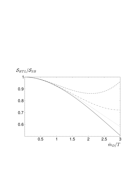
FIG. 7.: The HTL entropy per gluonic degree of freedom normalized to its Stefan-Boltzmann value as a function of the Debye mass $\hat{m}_{D}(T,\mu)/T$. The full line gives the complete numerical result corresponding to Eq. (132); the dashed line corresponds to the perturbative result to order $(\hat{m}_{D}/T)^{3}\sim g^{3}$. The dotted line gives the entropy for scalar degrees of freedom with momentum-independent mass $m=m_{\infty}=\hat{m}_{D}/\sqrt{2}$; its perturbative approximant is given by the dash-dotted line.

On the other hand, the full numerical result for the HTL entropy (full line in Fig. 7) turns out to be a monotonously decreasing function of $\hat{m}_{D}/T$. In the case of Eq. (184), the numerical evaluation involves solving first numerically the transcendental equations for $\omega_{T}(k)$ and $\omega_{L}(k)$, and a numerical integration, in which it is advisable to separate off the Stefan-Boltzmann value through the replacement $\log[1-e^{-\omega_{T}(k)/T}]\to\log[(1-e^{-\omega_{T}(k)/T}/(1-e^{-k/T})]$; Eq. (186) requires two successive numerical integrations.

It is interesting to compare the rather complicated expression ${\cal S}_{HTL}$ with the simple scalar expression Eq. (47) of the entropy of an ideal gas of massive bosons, $2N_{g}{\cal S}_{0}(m)$, which is basically what is considered in the simple massive quasiparticle models of Ref. [5, 6]. If in the latter the boson masses are identified with the asymptotic mass of the gluons, $m=m_{\infty}=\hat{m}_{D}/\sqrt{2}$, then this reproduces the correct leading-order interaction term in the entropy. The plasmon effect (i.e. the order-$g^{3}$ contribution) is included only partially, but not as $1/4$ of the complete plasmon effect, but as $1/(4\sqrt{2})$. This is because a constant thermal mass equal to its asymptotic value underestimates the Debye mass by a factor of $1/\sqrt{2}$ and therefore the plasmon effect by $(1/\sqrt{2})^{3}$, which is only partially compensated by now having $2N_{g}$ degrees of freedom exhibiting the analog of Debye screening instead of only the $N_{g}$ longitudinal ones.

Numerically, $2N_{g}{\cal S}_{0}(m_{\infty})$ reproduces the HTL entropy very accurately (within $\lesssim 0.1\%$) up to $\hat{m}_{D}\approx T$. For larger values of $\hat{m}_{D}$, the HTL entropy leads to significantly larger deviations from ${\cal S}_{SB}$. This latter fact is somewhat surprising since the plasmon effect, which in the HTL entropy is 30% greater than in the simple massive quasiparticle entropy, always counteracts the leading-order interaction contribution, as can be seen from the perturbative approximant of $2N_{g}{\cal S}_{0}(m_{\infty})$ (dash-dotted line in Fig. 7) and that of the HTL entropy (dashed line) through order $g^{3}$. This is partly due to the fact that ${\cal S}_{HTL}$ contains also a term $\sim g^{4}\log(c/g)$, which is not present in the simple massive quasiparticle entropy $2N_{g}{\cal S}_{0}(m_{\infty})$.

FIG. 8.: Relative deviation of the HTL entropy from that of a gas of massive bosons with (constant) mass $m_{\infty}$ (full line). The relative deviation of just the transverse quasiparticle contribution is given by the uppermost dash-dotted line; the transverse Landau-damping contribution is given by the lower dash-dotted line. The short-dashed line gives the longitudinal quasiparticle contribution; the long-dashed line the longitudinal Landau-damping one.

Inspecting in more detail the numerical deviation of the HTL entropy from that of a massive gas of bosons, one finds that the quasiparticle contribution from the transverse modes, which is always the dominant contribution to the entropy, by itself is always above $2N_{g}{\cal S}_{0}(m_{\infty})$. The transverse Landau-damping contribution is also positive, but relatively smaller. On the other hand, both the longitudinal quasiparticle and Landau-damping contributions are negative, resulting in a small net deviation from the simple massive boson entropy for small values of $\hat{m}_{D}/T$. When normalized to the deviation of $2N_{g}{\cal S}_{0}(m_{\infty})$ from the Stefan-Boltzmann result, the deviation of ${\cal S}_{HTL}$ from $2N_{g}{\cal S}_{0}(m_{\infty})$ is less than about +1% for $\hat{m}_{D}/T<0.739$, while negative and rapidly growing for larger values of $\hat{m}_{D}/T$, as shown in Fig. 8.

The formulae for the fermionic contributions to the entropy are quite analogous to the gluonic contributions. They read ${\cal S}_{f,HTL}={\cal S}_{f,HTL}^{\rm QP}+{\cal S}_{f,HTL}^{\rm LD}$ with

$${\cal S}_{f,HTL}^{\rm QP} = NN_{f}\int\limits_{0}^{\infty}{k^{2}dk\over\pi^{2}}{\partial\over\partial T}\Bigl{\{}T\log(1+\epsilon^{-[\omega_{+}(k)-\mu]/T})$$ (188)

$$\qquad\qquad\qquad+T\log{1+\epsilon^{-[\omega_{-}(k)-\mu]/T}\over 1+\epsilon^{-(k-\mu)/T}}+(\mu\to-\mu)\Bigr{\}}$$

where again only the explicit $T$ dependences are to be differentiated and not those implicit in the dispersion laws $\omega_{+}(k)$ and $\omega_{-}(k)$ of the fermionic quasiparticles, which are given by the solutions of $\omega_{\pm}=\pm[p+\hat{\Sigma}_{\pm}(\omega_{\pm},k)]$ with $\hat{\Sigma}_{\pm}$ given by Eq. (167).

FIG. 9.: The HTL entropy per quark degree of freedom at $\mu=0$ normalized to its free value as a function of the fermionic plasma frequency $\hat{M}/T$. The full line gives the complete numerical result corresponding to Eq. (155) in the HTL approximation; the dashed line corresponds to the perturbative result to order $(\hat{M}/T)^{2}\sim g^{2}$; the dotted line gives the entropy for a fermionic degree of freedom with momentum-independent mass $M=M_{\infty}=\sqrt{2}\hat{M}$, which has the same perturbative approximant to order $g^{2}$.

The fermionic Landau-damping contribution to the entropy is

$${\cal S}_{f,HTL}^{\rm LD}=-NN_{f}\int\limits_{0}^{\infty}{k^{2}dk\over\pi^{3}}\int\limits_{0}^{k}\!d\omega\left[{\partial f_{+}(\omega)\over\partial T}+{\partial f_{-}(\omega)\over\partial T}\right]\Bigl{\{}\arg[k-\omega+\hat{\Sigma}_{+}(\omega,k)]$$ (189)

$$\qquad\qquad\qquad\qquad\qquad\quad-{\,\mathrm{I}m\,}\hat{\Sigma}_{+}(\omega,k){\,\mathrm{R}e\,}[k-\omega+\hat{\Sigma}_{+}(\omega,k)]^{-1}$$ (190)

$$\qquad\quad+\,\arg[k+\omega+\hat{\Sigma}_{-}(\omega,k)]-{\,\mathrm{I}m\,}\hat{\Sigma}_{-}(\omega,k){\,\mathrm{R}e\,}[k+\omega+\hat{\Sigma}_{-}(\omega,k)]^{-1}\Bigr{\}}$$ (191)

In the case of the gluonic contributions to the HTL entropy, there was no difference between vanishing and non-zero chemical potential other than the resulting different value of $\hat{m}_{D}$, which depends on $\mu$ according to Eq. (145). For the quark contributions to the entropy, the chemical potential enters both explicitly through the Fermi-Dirac distribution function $f$ and through the magnitude of the fermionic plasma frequency $\hat{M}$.

In Fig. 9 the results of a numerical evaluation of the fermionic contribution to the HTL entropy normalized to its free value is given as a function of $\hat{M}/T$ for $\mu=0$. When compared with the free entropy of simple massive fermions of mass $M=M_{\infty}=\sqrt{2}\hat{M}$, one finds that the HTL entropy exceeds the latter by at most +1.2% for $\hat{M}/T\approx 1$, coincides with it at $\hat{M}/T\approx 1.39$, and becomes lower for larger $\hat{M}/T$. On the other hand, the strictly perturbative result up to order $g^{2}$ is significantly lower, but compared to the gluonic contribution the discrepancy is much smaller because there is no (direct) plasmon effect in the fermionic contributions [all order $g^{3}$ contributions eventually arise from NLO corrections to $M_{\infty}$].

Turning now to the quark density, its quasiparticle and Landau-damping contributions are obtained by replacing $\partial/\partial T$ in the above formulae (188,189) by $\partial/\partial\mu$.

In the limit $T\to 0$, the resulting expressions can be simplified to read (for $\mu>0$)

$${\cal N}_{HDL}^{\rm QP}\Big{|}_{T=0}=NN_{f}\int\limits_{0}^{\mu}{k^{2}dk\over\pi^{2}}[\theta(\mu-\omega_{+}(k))-\theta(\omega_{-}(k)-\mu)].$$ (192)

and

$${\cal N}_{HDL}^{\rm LD}\Big{|}_{T=0} = -NN_{f}\int\limits_{\mu}^{\infty}{k^{2}\,dk\over\pi^{3}}\Bigl{\{}\arg[k-\mu+\hat{\Sigma}_{+}(\mu,k)]$$ (195)

$$\qquad\qquad\qquad\qquad-{\,\mathrm{I}m\,}\hat{\Sigma}_{+}(\mu,k){\,\mathrm{R}e\,}[k-\mu+\hat{\Sigma}_{+}(\mu,k)]^{-1}$$

$$\qquad+\,\arg[k+\mu+\hat{\Sigma}_{-}(\mu,k)]-{\,\mathrm{I}m\,}\hat{\Sigma}_{-}(\mu,k){\,\mathrm{R}e\,}[k+\mu+\hat{\Sigma}_{-}(\mu,k)]^{-1}\Bigr{\}}.$$

For $\mu>\hat{M}$, the quasiparticle contribution (192) can be more explicitly written as

$${\cal N}_{HDL}^{\rm QP}/NN_{f}\Big{|}_{T=0,\mu>\hat{M}}={\mu^{3}\over 3\pi^{2}}-{1\over 3\pi^{2}}\left[\mu^{3}-k_{+}^{3}(\mu)\right]-{1\over 3\pi^{2}}\left[\mu^{3}-k_{-}^{3}(\mu)\right]$$ (196)

where $k_{\pm}(\mu)$ is the solution of $\omega_{\pm}(k_{\pm})=\mu$.

The first term on the right-hand side of Eq. (196) represents the free contribution of one massless Dirac fermion, the two bracketed terms are the corrections from the nontrivial dispersion laws of the two fermionic quasiparticle branches.

For comparison, the fermion density of a free massive Dirac fermion with mass $M$ is given by

$${\cal N}_{0}(M)\Big{|}_{T=0}=\left\{\begin{array}[]{c@{\quad\rm for\quad}l}{1\over 3\pi^{2}}(\mu^{2}-M^{2})^{3/2}&\mu>M\\ 0&\mu<M\end{array}\right.$$ (197)

Identifying $M=M_{\infty}=\sqrt{2}\hat{M}$ gives the correct leading-order interaction term of order $g^{2}$, while leading to somewhat larger values for ${\cal N}$ than the perturbative order-$g^{2}$ result for all $\hat{M}/\mu$.

FIG. 10.: The HDL quark density per quark degree of freedom at $T=0$ normalized to its free value as a function of the fermionic plasma frequency $\hat{M}/\mu$. The full line gives the complete numerical result corresponding to Eq. (157) in the HDL approximation; the dashed line corresponds to the perturbative result to order $(\hat{M}/\mu)^{2}\sim g^{2}$; the dotted line gives the density for a fermionic degree of freedom with momentum-independent mass $M=M_{\infty}=\sqrt{2}\hat{M}$, which has the same perturbative approximant to order $g^{2}$, and vanishes for $M\geq\mu$, i.e. $\hat{M}/\mu\geq 1/\sqrt{2}$.

In Fig. 10 the numerical result for ${\cal N}_{HDL}$ at $T=0$ is plotted for $\hat{M}/\mu$ up to $1/\sqrt{2}$, where the fermion density of Eq. (197), displayed by the dotted line, vanishes. The HDL result, which is given by the full line, is seen to drop to zero almost at the same ratio, to wit, $\hat{M}/\mu\approx 0.69264$. Beyond this point the result becomes negative, showing that the approximation is breaking down at such high values of $\hat{M}/\mu$. [Note that, since $\hat{M}^{2}=g^{2}\mu^{2}/6\pi^{2}$ for $N=3$ and $T=0$ (cf. Eq. (168)), $\hat{M}/\mu\approx 0.69$ corresponds to a relatively large coupling $g\approx 5.3$.]

For comparison, the strictly perturbative result to order $g^{2}$ is given by the dashed line in Fig. 10, which is seen to approach zero faster than the HDL density as well as that of a simple massive quasiparticle.

B Estimate of NLO contributions

As we have discussed at length in the previous sections, the HTL approximation in the entropy contains only part of the plasmon effect, a different source of order $g^{3}$ contributions comes from NLO corrections to the gluonic and fermionic self-energies at hard momenta on the light-cone as given by Eq. (179). From the result (III D 3) we know that this NLO contribution corresponds precisely to the second term of the right-hand side of Eq. (180).

In the case of the density, it is clear from the absence of a bosonic distribution function in Eq. (157) that ${\cal N}$ in the HTL/HDL approximation does not contain any $g^{3}$ contribution, so all of ${\cal N}_{3}$ as given by Eq. (182) arises from the NLO correction to the quark self-energy at hard momenta on the light-cone.

As can be seen e.g. from Eqs. (A20) and (A22), the NLO self-energy corrections are complicated and nonlocal quantities. Even when evaluated on the light-cone, they do not simply give a constant correction to the asymptotic mass, but a nontrivial function of the (hard) momentum. In fact, there are even contributions of the form $g^{2}\hat{m}_{D}p$, which grow larger than $g^{3}T^{2}$ for $p\gg T$, eventually causing a break-down of standard HTL perturbation theory, but fortunately such contributions are irrelevant thanks to the fact that $n(p)$ shuts off exponentially then.

Because a full inclusion of the NLO self-energy corrections is rather complicated and computationally expensive, and because in the applications below the magnitude of the NLO corrections, when treated along the lines of the scalar toy model in Sect. II D, turns out to be comparatively small, we shall in the following consider the approximation of an effective constant NLO asymptotic mass. The complete evaluation of $\delta\Pi$ and $\delta\Sigma$, which involves a number of technical intricacies, will be reserved for a separate publication. Their eventual numerical effects on the thermodynamic potentials is work in progress, though we do not expect them to deviate too much from the estimates derived in this subsection.

From the requirement that a replacement of $m_{\infty}^{2}$ and $M_{\infty}^{2}$ in Eqs. (105), (173), and (174) by effective constant (i.e. averaged) corrections $\bar{\delta}m_{\infty}^{2}$ and $\bar{\delta}M_{\infty}^{2}$ equals ${\cal S}_{3}^{\mathrm{h}ard}$ and ${\cal N}_{3}^{\mathrm{h}ard}={\cal N}_{3}$ (cf. Eqs. (180) and (182), respectively), we have

$$-{1\over 6}N_{g}\bar{\delta}m_{\infty}^{2}T-{1\over 6}NN_{f}\bar{\delta}M_{\infty}^{2}T = {1\over 4\pi}N_{g}\hat{m}_{D}m_{T}^{2}$$ (198)

$$-{1\over 2\pi^{2}}NN_{f}\bar{\delta}M_{\infty}^{2}\mu = N_{g}{T\over 4\pi\mu}\hat{m}_{D}m_{\mu}^{2}$$ (199)

with $\hat{m}_{D}$, $m_{T}$, and $m_{\mu}$ as defined in Eq. (181). This has the remarkably simple unique solution

$$\bar{\delta}m_{\infty}^{2}=-{1\over 2\pi}g^{2}NT\hat{m}_{D},\quad\bar{\delta}M_{\infty}^{2}=-{1\over 2\pi}g^{2}C_{f}T\hat{m}_{D},$$ (200)

where in the latter $C_{f}=N_{g}/(2N)$. Indeed, in Eq. (200) both the dependence on the Casimirs $N$ and $C_{f}$ as well as their proportionality to $\hat{m}_{D}$ is in accordance to one’s expectations from the form of the corresponding HTL-resummed one-loop diagrams of Figs. 4 and 6, respectively.

However, in complete analogy to the scalar toy model of Sect. II D, we find that the magnitude of the corrections to the asymptotic masses are such that $m_{\infty}^{2}+\bar{\delta}m_{\infty}^{2}$ drops to negative values for $g\gtrsim 1$, which would give rise to tachyonic singularities in the semi-perturbative entropy result (for $N=3$ and $\mu=0$ the naive strictly perturbative mass is again given by the shorter-dashed line in Fig. 1). For slightly higher values of $\hat{m}_{D}/T\sim g$, the same phenomenon occurs with $M_{\infty}^{2}+\bar{\delta}M_{\infty}^{2}$.

In the scalar model we have seen that including the NLO correction to the thermal mass in the approximately self-consistent form (74) gives instead a monotonously growing function in $g$ and very good agreement with the exact result in the $N\to\infty$ limit even for large $g$. For QCD, we define in analogy to Eq. (74) the NLA asymptotic mass through the quadratic equation

$$\bar{m}_{\infty}^{2}={g^{2}(N+N_{f}/2)T^{2}\over 6}-{g^{2}NT\over\sqrt{2}\pi}\bar{m}_{\infty}$$ (201)

and similarly for $\bar{M}_{\infty}^{2}$.

In contrast to the scalar case, however, where the thermal mass and its NLO correction was momentum-independent and therefore applicable for all momenta, the results (200) apply only at hard momenta. Indeed, NLO corrections to thermal masses in QCD as far as they have been calculated turn out to be rather different at soft momenta: In Ref. [36], the NLO correction for the plasma frequency of pure-glue QCD in the long-wavelength limit has been calculated with the result $\delta m^{2}_{pl.}/\hat{m}^{2}_{pl.}\approx-0.18\sqrt{N}g$, which is only about a third of the relative (averaged) correction of $m^{2}_{\infty}$. Moreover, the Debye mass turns out to even receive positive corrections [37] $\delta m^{2}_{D}/\hat{m}^{2}_{D}=+\sqrt{3N}/(2\pi)\times g\log(c/g)$, with recent lattice simulations [38] yielding a rather large constant $c$.

For this reason we choose to leave the HTL results for the soft gluonic propagators and self-energies completely untouched, and we implement the NLO correction to the asymptotic mass by introducing a cutoff scale that separates hard from soft momenta at a scale $\Lambda=\sqrt{2\pi T\hat{m}_{D}c_{\Lambda}}$ which is proportional to the geometric mean of the hard Matsubara scale $2\pi T$ and a soft scale $c_{\Lambda}\hat{m}_{D}$. For momenta $k\leq\Lambda$ we keep the HTL approximation and for $k\geq\Lambda$ we take the thermal gluons to have the constant asymptotic mass $\bar{m}_{\infty}^{2}$ of Eq. (201). This completes the definition of our present next-to-leading approximation to the entropy ${\cal S}_{NLA}$.

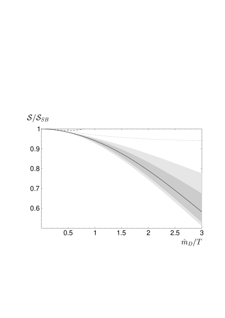
FIG. 11.: The NLA entropy obtained by including $\bar{\delta}m_{\infty}$ according to Eq. (201) for hard momenta $k\geq\Lambda=\sqrt{2\pi T\hat{m}_{D}c_{\Lambda}}$ in the pure-glue entropy. The central line in the shaded areas corresponds to $c_{\Lambda}=1$, the two differently shaded areas to the bands $c_{\Lambda}={1\over 2}\ldots 2$ and $c_{\Lambda}={1\over 4}\ldots 4$, respectively. The dotted line corresponds to a simple scalar model with constant mass $m$ modified according to Eq. (202) such that it also contains the perturbative pure-glue result up to and including order $g^{3}$; the latter is displayed by the dashed line that leaves the plot already at $\hat{m}_{D}/T\approx 0.785$.

In Fig. 11, the numerical result for pure-glue QCD with $c_{\Lambda}=1$ is given by the full line. The effect of varying $c_{\Lambda}$ in the range ${1\over 2}\ldots 2$, which keeps $\Lambda$ well in between the interval $(\hat{m}_{D},2\pi T)$ for all values of $\hat{m}_{D}/T$, is displayed by the dark-grey band; the more extreme variation $c_{\Lambda}={1\over 4}\ldots 4$ extends the latter by the light-grey areas. We shall see, however, that in the eventual applications to QCD at temperatures a few times the transition temperature the resulting increase in our “theoretical error” will be still moderate when compared to the renormalization scheme dependences.

For the sake of comparison with a simpler quasiparticle model, the dotted line in Fig. 11 shows the entropy of two interaction-free scalar bosons with constant mass

$$\bar{m}^{2}={1\over 2}\hat{m}_{D}^{2}\left(1-{4\sqrt{2}-1\over\pi}{\bar{m}\over T}\right)$$ (202)

which mimicks the NLA result (201), but adjusted such as to reproduce the perturbative QCD result up to and including order $g^{3}$ in this simpler model.

In the fermionic quantities ${\cal S}_{f}$ and ${\cal N}$, which because of the absence of Bose enhancement are less sensitive to the soft scale, we implement the fermionic analog of Eq. (201) by rescaling $\hat{M}^{2}$ at all momenta for simplicity (as in the scalar case in Sect. II.D).

C Renormalization-group improvement

In the HTL/HDL approximation, all the gluonic and fermionic contributions above depend on the numerical value of the HTL/HDL masses $\hat{m}_{D}^{2}$ and $\hat{M}^{2}$, respectively, which are proportional to $\alpha_{s}=g^{2}/4\pi$. The latter is a renormalization scheme and renormalization scale $(\bar{\mu})$ dependent quantity, and so are therefore our results for entropy and density. Following Ref. [4] we adopt modified minimal subtraction and assume that an optimal choice of the renormalization scale should be found around the scale of the Matsubara frequencies, $2\pi T$, or in the case of zero temperature and finite density around the scale of the diameter of the Fermi sphere, $2\mu$. After all, the hard thermal/dense loops are generated by hard excitations, as are in fact the NLO contributions to the asymptotic masses within HTL/HDL perturbation theory.

Exactly as done in Ref. [11] in a direct HTL resummation of the thermodynamic pressure, we put in the running of the coupling by hand and choose it to be determined by the 2-loop renormalization group equation according to

$$\alpha_{s}(\bar{\mu})={4\pi\over\beta_{0}\bar{L}(\bar{\mu})}\left(1-{2\beta_{1}\log(\bar{L}(\bar{\mu}))\over\beta_{0}^{2}\bar{L}(\bar{\mu})}\right)$$ (203)

with $\bar{L}(\bar{\mu})=\log(\bar{\mu}^{2}/\Lambda^{2}_{\overline{\mathrm{M}S}})$ and

$$\beta_{0}=(11N-2N_{f})/3,\quad\beta_{1}=(34N^{2}-13NN_{f}+3N_{f}/N)/6.$$ (204)

1 Entropy

At least at zero density, lattice results relate the QCD scale parameter $\Lambda_{\overline{\mathrm{M}S}}$ to the critical temperature $T_{c}$, which in accordance with Ref. [39] we choose as $T_{c}=1.14\Lambda_{\overline{\mathrm{M}S}}$, both for pure-glue QCD and also for $N_{f}\not=0$, since lattice data indicate only a weak dependence of the ratio $T_{c}/\Lambda_{\overline{\mathrm{M}S}}$ on the number of quark flavor.

Putting $\bar{\mu}=c_{\bar{\mu}}2\pi T$ in Eq. (203) and assuming $c_{\bar{\mu}}\sim 1$ prescribes reasonably small values for $\alpha_{s}$ and thus for $\hat{m}_{D}/(2\pi T)$ and $\hat{M}/(\pi T)$ for all $T>T_{c}$ so as to make it interesting to compare the above HTL and NLA expressions with nonperturbative results from lattice gauge theory. Indeed, we have found that, for $\hat{m}_{D}\ll 2\pi T$ and $\hat{M}\ll\pi T$, the deviation from the free Stefan-Boltzmann result is small enough to make a semi-perturbative picture minimally tenable, although it is clear that the physics of the phase transition itself is completely beyond reach. On the other hand, the strictly perturbative results up to and including the order $g^{3}$ are such that entropy and pressure would be much higher than their Stefan-Boltzmann values, indicating a complete loss of convergence of strict thermal perturbation theory.

In order to have some indication of the theoretical uncertainty involved, we consider, again as done in Ref. [11], a variation of the renormalization scale by a factor of $c_{\bar{\mu}}={1\over 2}\ldots 2$.

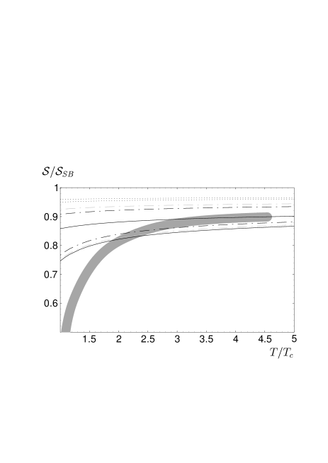
FIG. 12.: Comparison of the HTL entropy (full lines), the NLA results for $c_{\Lambda}={1\over 2}\ldots 2$ (dash-dotted lines) as well as $c_{\Lambda}={1\over 4}\ldots 4$ (gray dash-dotted lines), and the free entropy of bosons with mass (202) such as to reproduce the correct perturbative plasmon effect (dotted lines), all with $\overline{\hbox{MS}}$ renormalization scale $\bar{\mu}=\pi T\ldots 4\pi T$, with the lattice result of Ref. [40] for pure SU(3) gauge theory (dark-gray band).

For purely gluonic QCD, the lattice results involve the least uncertainties. In Ref. [40], the thermodynamic potentials of pure SU(3) gauge theory have been calculated from plaquette action densities on lattices up to $8\times 32^{3}$ for temperatures up to about $4.5T_{c}$ and extrapolating to the continuum limit by comparing different lattice sizes. The lattice result for the entropy density is rendered in Fig. 12 by a grey band whose thickness is meant to give a rough idea of the errors reported in Ref. [40].

Our result for the HTL entropy as displayed in Fig. 7 translates into a range of values bounded by the choices $\bar{\mu}=\pi T$ (lower full line) and $\bar{\mu}=4\pi T$ (upper full line). This already gives a remarkably good approximation of the lattice result for $T\gtrsim 2T_{c}$, somewhat underestimating the values at higher temperatures. In all of this the parameter $\hat{m}_{D}/T$ takes on values in the range $\sim 1\ldots 2$, where we have found the entropy of simple massive bosons to give only slightly larger results (cf. Fig. 7).

Now the HTL entropy contains only part (here 1/4) of the plasmon effect. The latter is completely included in the NLA entropy as defined after Eq. (201). In Fig. 12, ${\cal S}_{NLA}$ is represented by the area bounded by the black dash-dotted lines, where the lower one corresponds to the choice $\bar{\mu}=\pi T$ and $c_{\Lambda}=2$, and the higher one to $\bar{\mu}=4\pi T$ and $c_{\Lambda}=1/2$. For this range of $c_{\Lambda}$ the scale $\Lambda$ remains well separated from both $\hat{m}_{D}$ and $2\pi T$ for all $T>T_{c}$. Extending the range of $c_{\Lambda}$ to $c_{\Lambda}=1/4\ldots 4$ gives the area bounded by the gray dash-dotted lines. Although $\Lambda$ now varies all the way from $\hat{m}_{D}$ to $2\pi T$, the error band is only moderately enlarged.

Evidently, the NLA estimates based upon Eq. (201) do not move away too much from the HTL results, which first of all is what is required to make our semi-perturbative procedure tenable. What is more, the results show a surprisingly good agreement with the lattice results for temperatures greater than 2…3 times the critical temperature.

Recently, in Ref. [41] the results of Ref. [40] have been reproduced within errors by using a renormalization-group improved lattice action for temperature up to $3.5T_{c}$. The results of Ref. [41] for the pressure are systematically higher by about 5…2% for temperatures 2…3.5$T_{c}$. For the entropy, which has not been extracted explicitly in Ref. [41], this would imply a result that is centered around the upper boundary of the grey band in Fig. 12 for $T\approx 3T_{c}$, and slightly flatter around $T\sim 2T_{c}$, all with slightly reduced error bars. If anything, the agreement with our HTL and NLA results appears to be even a bit improved.

Comparing finally with the entropy of free massive bosons with mass according to Eq. (202) such as to reproduce the correct perturbative plasmon effect, this is included in Fig. 12 as the band bounded by the dotted lines corresponding to $\bar{\mu}=\pi T\ldots 4\pi T$. Since the renormalization scale dependence decreases with decreasing deviation from the Stefan-Boltzmann value, this band is rather narrow. It is also clearly in lesser agreement with the lattice data, which thus favor the momentum-dependent inclusion of NLO corrections to the thermal masses that follows from NLO perturbation theory and that we have modelled in our NLA estimates.

In Fig. 13, the central results for the HTL and NLA entropy ($\bar{\mu}=2\pi T$ and $c_{\Lambda}=1$) are displayed together with the results for $N_{f}=2$ and 3. Only a rather weak dependence on $N_{f}$ is found in this (greatly magnified) plot where the entropy is normalized to the free value, and $T$ to the respective ($N_{f}$-dependent) $T_{c}\propto\Lambda_{\overline{\hbox{MS}}}$.

These results are in good agreement with recent lattice results[42] for $N_{f}=2$ and their estimated extrapolation to the continuum limit and to the limit of massless quarks as we have already noted in Ref. [16]. In Fig. 13, a conversion of the lattice result to the entropy is included as a gray band, and, indeed, for $T/T_{c}\gtrsim 2.5$ our NLA estimate turns out to lie close to the center of the estimated error band of the lattice result.

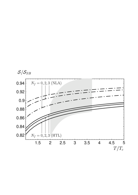
FIG. 13.: Comparison of the HTL entropy (full lines) and the NLA result with $c_{\Lambda}=1$ (dash-dotted lines) for flavor numbers $N_{f}=0,2,3$, all with the central choice of $\overline{\hbox{MS}}$ renormalization scale $\bar{\mu}=2\pi T$. The estimate of a continuum extrapolation of the lattice result for $N_{f}=2$ as reported in Ref. [42, 43] and its estimated error, converted to ${\cal S}/{\cal S}_{SB}$, is given by the gray band. Notice the blown-up scale of the ordinate compared to Fig. 12.

The further result that for $N_{f}=3$ our NLA estimate for ${\cal S}/{\cal S}_{SB}$ as a function of $T/T_{c}$ is approximately the same fits nicely to the recent lattice data for $N_{f}=3$ [43], which are consistent with a coincidence of the asymptotic values of $P/P_{SB}$ and also for ${\cal S}/{\cal S}_{SB}$. A more detailed comparison of our results with the lattice data, in particular at smaller temperatures, is hardly worthwhile in view of the large uncertainties associated with the extrapolation to the massless continuum limit.

In our previous works [15, 16] we have been considering a simple Padé-improved inclusion of the NLO asymptotic mass correction in place of the NLA form (201). A comparison of the respective results shows that our estimate of the effects of an approximately self-consistent treatment of NLO corrections to the self-energies is fairly robust, with the main uncertainties coming from the choice of the renormalization scale.

2 Density

For nonvanishing chemical potential, where lattice data are missing to determine precisely the critical temperature or density in terms of $\Lambda_{\overline{\mathrm{M}S}}$, we can nevertheless translate our results into functions of $T/\Lambda_{\overline{\mathrm{M}S}}$ and $\mu/\Lambda_{\overline{\mathrm{M}S}}$ provided we choose the renormalization scale $\bar{\mu}$ as a suitable combination of $T$ and $\mu$. If, as we have assumed, the spacing of the Matsubara frequencies, $2\pi T$, gives a good choice for the renormalization scale $\bar{\mu}$ at zero density, it seems plausible to adopt the diameter of the Fermi sphere, $2\mu$, in the case of zero temperature. This choice of a relative factor of $\pi$ is particularly natural when considering the form of the leading-order result for the fermionic thermal masses, Eq. (168), where $T$ and $\mu/\pi$ appear on equal footing.

In Fig. 14 we give the numerical results for the quark density ${\cal N}_{HDL}$ at $T=0$ for $N=3$ and $N_{f}=3$ as a function of $\mu/\Lambda_{\overline{\mathrm{M}S}}$ for the range $\bar{\mu}=\mu\ldots 4\mu$. In this case we do not attempt to include NLO corrections, for they do not contribute terms of order $g^{3}$. NLO corrections to the hard fermion self-energy are in fact responsible for completing the plasmon effect at order $g^{4}\log(g)$, but a complete calculation of the former would be needed to determine that part of the constant under the logarithm that comes from the spectral properties of quasiparticles rather than explicit order-$g^{4}$ interactions, which are dropped in the approximation ${\cal N}^{\prime}=0$.

The dashed line in Fig. 14 gives the strictly perturbative result at order $g^{2}$. The result corresponding to a simple quasiparticle model with mass $M=M_{\infty}$ is not included; from Fig. 10 it is clear that it is in between the HDL result and the order-$g^{2}$ one, and somewhat closer to the latter.

The perturbative result up to and including order $g^{4}$ has been calculated by Freedman and McLerran [34] and by Baluni [45]. However, it has been obtained in a particular momentum subtraction scheme. In order to convert this to the gauge-independent $\overline{\hbox{MS}}$ scheme, one should replace the scale parameter $\mu_{0}$ in Ref. [34] ($M$ in Refs. [45, 1]) according to

$$\mu_{0}=\bar{\mu}\exp\left\{[(151+36\alpha+9\alpha^{2})N-40N_{f}]/[24(11N-2N_{f})]\right\},$$ (205)

where $\alpha$ is the gauge parameter used in the momentum subtraction scheme calculation. In particular for $N=3$ and uniform chemical potentials one finds

$$P/P_{0} = 1-2{\alpha_{s}(\bar{\mu})\over\pi}-\Bigl{[}10.347-0.536N_{f}+N_{f}\log{N_{f}\alpha_{s}(\bar{\mu})\over\pi}$$ (207)

$$\qquad\qquad\qquad\qquad\qquad\qquad+\;(11-{2\over 3}N_{f})\log{\bar{\mu}\over\mu}\;\Bigr{]}({\alpha_{s}(\bar{\mu})\over\pi})^{2}+O(\alpha_{s}^{3}),$$

$${\cal N}/{\cal N}_{0} = 1-2{\alpha_{s}(\bar{\mu})\over\pi}-\Bigl{[}7.597-0.369N_{f}+N_{f}\log{N_{f}\alpha_{s}(\bar{\mu})\over\pi}$$ (209)

$$\qquad\qquad\qquad\qquad\qquad\qquad+\;(11-{2\over 3}N_{f})\log{\bar{\mu}\over\mu}\;\Bigr{]}({\alpha_{s}(\bar{\mu})\over\pi})^{2}+O(\alpha_{s}^{3}).$$

With $N_{f}=3$, this is included in Fig. 14 by the dotted lines. Although the perturbative order-$g^{4}$ result constitutes a substantial correction of the order-$g^{2}$ result, perturbation theory at zero temperature and high densities is clearly much better behaved than at high temperatures—the interaction terms are increased by less than 50% for $\mu\gtrsim 2\Lambda_{\overline{\mathrm{M}S}}$ ($\mu\gtrsim 3\Lambda_{\overline{\mathrm{M}S}}$ in the case of $P/P_{0}$).

FIG. 14.: The result for the quark density for $N_{f}=3$ in the HDL approximation for $\bar{\mu}=\mu\ldots 4\mu$ (full lines) compared with the perturbative results at order $g^{2}$ (dashed lines) and order $g^{4}$ (dotted lines).

On the other hand, the nonperturbative ${\cal N}_{HDL}$ result is rather close to the perturbative order-$g^{2}$ result, showing even a slight decrease of the interaction contribution compared to the latter. The ${\cal N}_{HDL}$ result contains already a fraction of the coefficient of the $\alpha_{s}^{2}\log(\alpha_{s})$ term, together with a subset of the true higher-order contributions. It would be interesting to see how an NLA calculation, which would complete the $g^{4}\log(g)$ coefficient, compares with the perturbative order-$g^{4}$ result. We intend to investigate that in future work.

VI Conclusions and outlook

We have shown that it is possible to perform a resummation of HTL’s which is free of overcounting and UV problems through approximately self-consistent calculations of the thermodynamical functions of QCD, without the need for thermal counterterms. The two-loop skeleton approximation for the free energy reduces to effectively one-loop expressions for the entropy and the density but with dressed propagators. With the latter approximated by the HTL/HDL propagators we reproduce correctly the leading-order interaction terms. In fact, the latter can be expressed entirely in terms of the asymptotic thermal mass. The so-called plasmon-effect contributions of order $g^{3}$ on the other hand are only partly accounted for by HTL self-energies and propagators; the remaining contributions arise, rather unconventionally, from NLO corrections to the self-energy of hard particles at the light-cone as given by standard HTL perturbation theory.

This is to be contrasted with a direct HTL resummation of the one-loop pressure [11]. There the plasmon effect is contained completely in the soft contributions, whereas the leading-order interaction terms are over-included and corrected only in a (very complicated) two-loop calculation.

We would like to recall that while the HTL and NLA approximations that we have considered are manifestly gauge independent, this is not the case for our starting point, the self-consistent $\Phi$-derivable two-loop order approximation itself. The corresponding gap equation would involve unphysical gauge dependent features as well as an incomplete lowest order $\beta$-function both of which enter at order $g^{4}$, i.e. beyond the perturbative accuracy of a two-loop approximation. These are automatically dropped in our current approximations. Further improvements, beyond our HTL and NLA approximations would require to also improve upon the self-consistent two-loop approximation. In order to achieve gauge independence in (approximately) self-consistent resummations one should obviously turn to approximations which include dressed vertices, using for instance the formalisms which have been developed long ago by de Dominicis and Martin [17] and also Freedman and McLerran [34]. The strategy, in principle, would be to include vertex corrections, together with increasingly better approximations for the quasiparticle propagators. That is, with increasing number of loops in $\Phi$, the building blocks in this scheme—the self-consistent propagators and vertices—should be also improved. However, a practical implementation of such a scheme in the case of nonabelian gauge theories seems to be hopelessly complicated. It is therefore gratifying that the approximate propagator renormalization that we have presented turns out to be already a good approximation.

In the expressions that we use for the entropy and density the main contribution comes from the vicinity of the light-cone where hard thermal loops remain accurate also at hard momenta and provide the asymptotic masses. We have proposed a procedure of including NLO corrections through approximately self-consistent corrections to the thermal masses of the hard excitations only. The NLO corrections to the asymptotic masses can be calculated more accurately by means of standard HTL perturbation theory, the details of which are postponed to a forthcoming publication.

The numerical evaluation of our results combined with a two-loop renormalization group improvement turn out to compare remarkably well with available lattice data at zero quark chemical potential, which supports the picture according to which much of the effects of the interactions in the quark-gluon plasma can be adequately described by means of weakly interacting gluonic and fermionic (HTL) quasiparticles.

Extensions of the present work which are in progress concern the evaluation for general $\mu>0$ and $T>0$, and the integration of entropy and density to the thermodynamic pressure $P(\mu,T)$, similarly to what has been done in simple quasiparticle models in Ref. [47] (see also [16]). Maxwell’s relations, which constitute the corresponding integrability conditions, are satisfied up to and including order $g^{3}$ upon inclusion of the NLO contributions; beyond that order they give constraints on a possible renormalization-group improvement and it seems interesting to further pursue the present approach of combining the physical content of the perturbatively derivable hard thermal/dense self-energies with nonperturbative expressions for entropy and density, which in self-consistent two-loop order approximations only depend on the spectral properties of quasiparticle excitations.

A The plasmon effect in the QCD entropy

In this Appendix, we shall explicitly verify that our approximation for the entropy (cf. Eqs. (III A) and (155)) contains indeed the right perturbative correction of order $g^{3}$. Recall that ${\cal S}_{3}$ involves two types of contributions: the LO entropy of the soft gluons (longitudinal and transverse; cf. Eqs. (117) and (119)), and the NLO entropy of the hard particles (transverse gluons and fermions), as determined by the corresponding NLO self-energies on the light-cone (cf. Eqs. (116) and (179)).

Our strategy will be as follows: In Sect. A.1, we shall rewrite the soft gluon entropy in a way which will be convenient later. Then, in Sects. A.2 and A.3 we shall compute the NLO self-energy $\delta\Pi_{T}$ of a hard transverse gluon, and the corresponding contribution $\delta{\cal S}_{T}$ to the entropy. This will complete the derivation of the plasmon effect for a purely gluonic plasma. The extension to a plasma with fermions will be finally considered, in Sect. A.4.

1 The entropy of soft gluons

From Eqs. (117) and (119), the order-$g^{3}$ contribution of the soft gluons reads

$${\cal S}_{3}^{\mathrm{s}oft} = -\int\!\!{d^{4}k\over(2\pi)^{4}}\,\frac{1}{\omega}\left\{{\,\mathrm{I}m\,}\Bigl{[}\log(1+D_{0}\hat{\Pi})-\hat{\Pi}D_{0}\Bigr{]}\,-\,{\,\mathrm{I}m\,}\hat{\Pi}{\,\mathrm{R}e\,}(\hat{D}-D_{0})\right\}$$ (A1)

$$= {\cal S}_{3}^{(a)}+\Delta{\cal S}_{3},$$ (A2)

where ${\cal S}_{3}^{(a)}=({\partial}P_{3}/\partial T)|_{\hat{m}_{D}}$ (cf. Eq. (114)), and $\Delta{\cal S}_{3}$ is defined in Eq. (135). In Sect. III D 3, we have mentioned that $\Delta{\cal S}_{3}$ has been numerically found to vanish, because of a compensation between the electric and the magnetic contributions to Eq. (135). In what follows, however, we shall not use this information, but rather consider separately these electric and magnetic contributions, and show how they combine with the corresponding contributions to the NLO entropy of the hard particles $\delta{\cal S}$. Specifically, we shall verify that the identity in Eq. (124) holds separately in the electric and the magnetic sector.

To this aim, it is convenient to rewrite Eq. (135) in a slightly different form by using ${\,\mathrm{I}m\,}\hat{\Pi}{\,\mathrm{R}e\,}\hat{D}={\,\mathrm{I}m\,}(\hat{\Pi}\hat{D})-{\,\mathrm{R}e\,}\hat{\Pi}{\,\mathrm{I}m\,}\hat{D}$, and then integrating the first term:

$$\int\!\!{d^{3}k\over(2\pi)^{3}}\int\frac{d\omega}{2\pi\omega}\,{\,\mathrm{I}m\,}\Bigl{(}\hat{\Pi}_{L}(\hat{D}_{L}-D_{L}^{(0)})\Bigr{)}\,=\,{\hat{m}_{D}^{2}\over 2}\int\!\!{d^{3}k\over(2\pi)^{3}}\left({1\over k^{2}}-{1\over{k^{2}+\hat{m}_{D}^{2}}}\right)\,=\,{\hat{m}_{D}^{3}\over{8\pi}}\,.$$ (A3)

This yields (with $\hat{\rho}_{L,T}=2{\,\mathrm{I}m\,}\hat{D}_{L,T}$, cf. Eq. (84)):

$$\Delta{\cal S}_{3}=N_{g}\int\!\!{d^{4}k\over(2\pi)^{4}}\,{1\over 2\omega}\left\{\hat{\rho}_{L}\Bigl{(}{\,\mathrm{R}e\,}\hat{\Pi}_{L}-\hat{m}_{D}^{2}\Bigr{)}-2\Bigl{(}\hat{\rho}_{T}-\rho_{T}^{(0)}\Bigr{)}{\,\mathrm{R}e\,}\hat{\Pi}_{T}\right\}\,\equiv\,\Delta{\cal S}_{L}^{(3)}+\Delta{\cal S}_{T}^{(3)}\,,$$ (A4)

where we have also used the following “sum-rule” (cf. Eq. (82)):

$$\int\frac{d\omega}{2\pi}\,\frac{\hat{\rho}_{L}(\omega,k)}{\omega}\,=\,\,\frac{1}{k^{2}}\,-\,\frac{1}{k^{2}+\hat{m}_{D}^{2}}\,.$$ (A5)

Given the complicated structure of the HTL self-energies and spectral functions, the integrals in Eq. (A4) cannot be further evaluated in closed form. But this is actually not needed: indeed, the cumbersome terms in these expressions will be shortly shown to cancel against similar terms in ${\cal S}_{3}^{\mathrm{h}ard}$, the order-$g^{3}$ contribution of the hard particles, to be computed below.

2 The NLO gluon self-energy

We shall now compute the NLO self-energy contribution $\delta\Pi_{T}$ of a hard transverse gluon. This is determined by the effective one-loop diagrams in Fig. 4 where one of the internal lines is a soft gluon ($L$ or $T$) with the HTL-dressed propagator $\hat{D}-D_{0}$ (the subtraction of the free propagator $D_{0}$ is ensures that the loop integral is saturated by soft momenta). The other line in each of these diagrams is hard and transverse, and therefore undressed.

We are interested only in the transverse projection of $\delta\Pi_{\mu\nu}$:

$$\delta\Pi(p)\equiv\delta\Pi_{T}(p)\equiv\,{1\over 2}\,(\delta^{ij}-\hat{p}^{i}\hat{p}^{j})\,\delta\Pi_{ij}(p).$$ (A6)

We write $\delta\Pi_{T}=\delta\Pi^{l}+\delta\Pi^{t}$, where the upper indices refer to the soft internal lines in these diagrams, and compute only the longitudinal contribution $\delta\Pi^{l}$ in more detail. (The calculation of the transverse contribution is completely analogous.) This involves two of the diagrams in Figs. 4: the tadpole $\delta\Pi^{l}_{a}$ and the non-local diagram $\delta\Pi^{l}_{b}\,$. The tadpole gives

$$\delta\Pi^{l}_{a} = -g^{2}N\int[{\rm d}k]\Bigl{(}\hat{D}_{L}(k)-D_{L}^{(0)}(k)\Bigr{)}=-g^{2}N\int\!\!{d^{4}k\over(2\pi)^{4}}\,\hat{\rho}_{L}(k_{0},k)n(k_{0})$$ (A7)

$$\simeq -g^{2}NT\int\!\!{d^{4}k\over(2\pi)^{4}}\,{1\over k_{0}}\,\hat{\rho}_{L}(k_{0},k)\,=\,-\,\frac{g^{2}NT\hat{m}_{D}}{4\pi}\,,$$ (A8)

where the Matsubara sum in the first line has been performed by using the spectral representation (82), and in the second line we have replaced $n(k_{0})\simeq T/k_{0}$ (as appropriate at soft energies), and then performed the energy integral with the help of the sum-rule (A5). The final result in Eq. (A7) is indeed of order $g^{2}T\hat{m}_{D}\sim g^{3}T^{2}$, as expected.

The non-local diagram in Fig. 4.b yields:

$$\Bigl{(}\delta\Pi_{b}^{l}\Bigr{)}_{ij}(p)\,=\,-2\,{g^{2}N\over 2}\int[{\rm d}k]\,(2p_{0}+k_{0})^{2}\,D^{(0)}_{ij}(p+k)\Bigl{(}\hat{D}_{L}(k)-D_{L}^{(0)}(k)\Bigr{)},$$ (A9)

where $D^{(0)}_{ij}(q)$ is the free magnetic propagator in the Coulomb gauge,

$$D^{(0)}_{ij}(q)\,=\,(\delta_{ij}-\hat{q}_{i}\hat{q}_{j})\,{-1\over q_{0}^{2}-q^{2}}\,,$$ (A10)

and the factor 2 in front of the integral reflects the two possible ways to choose the soft longitudinal line among the two internal lines in the original one-loop diagram.

The transverse projection of Eq. (A9) involves ${1\over 2}\,(\delta^{ij}-\hat{p}^{i}\hat{p}^{j})(\delta_{ij}-\hat{q}_{i}\hat{q}_{j})$, where ${\bf q}={\bf k+p}$. Since $p\sim T$, we have $\hat{q}_{i}={p_{i}+k_{i}\over|{\bf p+k}|}\simeq\hat{p}_{i}$, while the integral in Eq. (A9) will be eventually dominated by soft $k$ momenta. In what follows, we shall often perform such kinematical simplifications relying on the fact that $k\ll p$. With this simplification, the product of the transverse projectors above reduces to the identity, so that

$$\delta\Pi_{b}^{l}(p)\,=\,-g^{2}N\int[{\rm d}k]\,(2p_{0}+k_{0})^{2}\,D_{0}(p+k)\Bigl{(}\hat{D}_{L}(k)-D_{L}^{(0)}(k)\Bigr{)}.$$ (A11)

To perform the Matsubara sum over $k_{0}$ we need the following sums (with ${\bf q}\equiv{\bf k+p}$):

$$T\sum_{k_{0}}D_{0}(p+k)\Bigl{(}\hat{D}_{L}(k)-D_{L}^{(0)}(k)\Bigr{)} = \int\!\!{dk_{0}\over 2\pi}\int\!\!{dq_{0}\over 2\pi}\,\hat{\rho}_{L}(k)\rho_{0}(q)\,{n(q_{0})-n(k_{0})\over k_{0}-q_{0}+p_{0}},$$ (A12)

$$T\sum_{k_{0}}k_{0}D_{0}(p+k)\Bigl{(}\hat{D}_{L}(k)-D_{L}^{(0)}(k)\Bigr{)} = \int\!\!{dk_{0}\over 2\pi}\int\!\!{dq_{0}\over 2\pi}\,k_{0}\,\hat{\rho}_{L}(k)\rho_{0}(q)\,{n(q_{0})-n(k_{0})\over k_{0}-q_{0}+p_{0}},$$ (A13)

$$T\sum_{k_{0}}k_{0}(k_{0}+p_{0})D_{0}(p+k)\Bigl{(}\hat{D}_{L}(k)-D_{L}^{(0)}(k)\Bigr{)} = \int\!\!{dk_{0}\over 2\pi}\int\!\!{dq_{0}\over 2\pi}\,k_{0}\,q_{0}\,\hat{\rho}_{L}(k)\rho_{0}(q)\,{n(q_{0})-n(k_{0})\over k_{0}-q_{0}+p_{0}}\,.$$ (A14)

This finally yields, for the retarded self-energy,

$$\delta\Pi_{b}^{l}(p)\,=\,-g^{2}N\int\!\!{d^{4}k\over(2\pi)^{4}}\int\!\!{dq_{0}\over 2\pi}\,\hat{\rho}_{L}(k)\rho_{0}(q)\,[4p_{0}^{2}+3p_{0}k_{0}+k_{0}q_{0}]\,{n(q_{0})-n(k_{0})\over k_{0}-q_{0}+p_{0}+i\epsilon}\,.$$ (A15)

To compute the entropy (116) we need the light-cone projection of the real part of this self-energy, ${\,\mathrm{R}e\,}\delta\Pi_{b}^{l}(p_{0}=p)$. Note that in previous calculations of the damping rate, it was rather the imaginary part of this same self-energy which was required [33, 48]. The calculation of the imaginary part is easier since the LO contribution $\sim g^{2}T^{2}$ can be immediately extracted from Eq. (A15) by neglecting $n(q_{0})\sim 1$ against $n(k_{0})\simeq T/k_{0}\gg 1$, and keeping only the large external momentum $4p_{0}^{2}$ in the numerator. This, together with

$${\,\mathrm{I}m\,}\,{1\over k_{0}-q_{0}+p_{0}+i\epsilon}\,=\,-\pi\delta(k_{0}-q_{0}+p_{0})\,\simeq\,-\pi\delta(k_{0}-k\cos\theta+p_{0}-p),$$ (A16)

leads to the following, standard, result for the longitudinal part of the damping rate [48] :

$$\gamma_{l}\,\equiv\,-\,{{\,\mathrm{I}m\,}\delta\Pi_{b}^{l}(p_{0}=p)\over 2p}\,=\,{g^{2}NT\over 2}\int\!\!{d^{3}k\over(2\pi)^{3}}\int\!\!{d\omega\over\omega}\,\hat{\rho}_{L}(\omega,k)\,\delta(\omega-k\cos\theta).$$ (A17)

If we perform, however, the same simplifications on the real part, then the would-be LO result turns out to vanish, by parity (with ${\bf P}$ denoting the principal value):

$$\Bigl{(}{\,\mathrm{R}e\,}\delta\Pi_{b}^{l}(p_{0}=p)\Bigr{)}_{naive}\,=\,g^{2}NT\int\!\!{d^{3}k\over(2\pi)^{3}}\int\!\!{d\omega\over\pi\omega}\,\hat{\rho}_{L}(\omega,k)\,\,{\bf P}\,{1\over\omega-k\cos\theta}\,=\,0\,.$$ (A18)

In fact, this is only to be expected: the terms in Eq. (A18) are formally of order $g^{2}T^{2}$, while we know that ${\,\mathrm{R}e\,}\delta\Pi$ should be rather of order $g^{3}T^{2}$. Thus, in order to extract the leading contribution to ${\,\mathrm{R}e\,}\delta\Pi$ from Eq. (A15) one has to push the kinematical approximations one step further as compared to the damping rate. In particular, we need the expansion of the statistical factors in Eq. (A15) to LO and NLO order:

$$n(k_{0})-n(q_{0})\simeq\,{T\over k_{0}}\,-\,{2n(q_{0})+1\over 2}\,.$$ (A19)

We shall denote by ${\,\mathrm{R}e\,}\delta\Pi_{b1}^{l}$ the contribution coming from $T/k_{0}\,$, and by ${\,\mathrm{R}e\,}\delta\Pi_{b2}^{l}$ the remaining one due to $(2n(q_{0})+1)/2$. These quantities will be evaluated at $p_{0}=p$, so they are functions of the three-momentum $p$ alone. We have:

$${\,\mathrm{R}e\,}\delta\Pi_{b1}^{l}(p) = g^{2}NT\int\!\!{d^{3}k\over(2\pi)^{3}}\int\!\!{dk_{0}\over 2\pi k_{0}}\,\hat{\rho}_{L}(k)\int\!\!{dq_{0}\over 2\pi}\,[4p^{2}+3pk_{0}+k_{0}q_{0}]\,{\bf P}\,{\rho_{0}(q)\over k_{0}-q_{0}+p}\,$$ (A20)

$$= g^{2}NT\int\!\!{d^{3}k\over(2\pi)^{3}}\int\!\!{dk_{0}\over 2\pi k_{0}}\,\hat{\rho}_{L}(k)(2p+k_{0})^{2}\,{\,\mathrm{R}e\,}D_{0}(p+k)\,,$$ (A21)

where in the second line we have identified the (retarded) free propagator via its spectral representation. In ${\,\mathrm{R}e\,}\delta\Pi_{b2}$, we can restrict ourselves to the LO term $4p^{2}$ in the denominator, and to the positive-energy pole $q_{0}=|{\bf p+k}|\simeq p+k\cos\theta$ in the spectral function $\rho_{0}(q_{0},|{\bf p+k}|)$. This yields:

$${\,\mathrm{R}e\,}\delta\Pi_{b2}^{l}(p) \simeq -g^{2}Np(2n(p)+1)\int\!\!{d^{4}k\over(2\pi)^{4}}\,{\hat{\rho}_{L}(k_{0},k)\over k_{0}-k\cos\theta}\,.$$ (A22)

3 The NLO entropy of hard gluons

Let us consider first a purely gluonic plasma, in which case the hard gluon self-energy $\delta\Pi_{T}=\delta\Pi^{l}+\delta\Pi^{t}$, is all what we need to compute the NLO entropy ${\cal S}_{3}^{\mathrm{h}ard}\equiv\delta{\cal S}^{l}+\delta{\cal S}^{t}$. As before, we focus on the longitudinal contribution $\delta{\cal S}^{l}$; by inserting Eqs. (A7), (A20) and (A22) in Eq. (116), we obtain $\delta{\cal S}^{l}=\delta{\cal S}_{1}^{l}+\delta{\cal S}_{2}^{l}$, where:

$$\delta{\cal S}_{1}^{l} \equiv -N_{g}\int\!\!{d^{4}p\over(2\pi)^{4}}\,\rho_{0}(p)\,{\partial n(p_{0})\over\partial T}\,\Bigl{[}\delta\Pi^{l}_{a}+{\,\mathrm{R}e\,}\delta\Pi_{b1}^{l}\Bigr{]}$$ (A23)

$$= -g^{2}NN_{g}T\int\!\!{d^{4}k\over(2\pi)^{4}}\,{\hat{\rho}_{L}(k)\over k_{0}}\int\!\!{d^{4}p\over(2\pi)^{4}}\,{\partial n(p_{0})\over\partial T}\,\rho_{0}(p)\,\Bigl{[}(2p+k_{0})^{2}\,{\,\mathrm{R}e\,}D_{0}(p+k)-1\Bigr{]}$$ (A24)

$$\simeq N_{g}T\int\!\!{d^{4}k\over(2\pi)^{4}}\,{\hat{\rho}_{L}(k)\over 2k_{0}}\,{\partial\over\partial T}{\,\mathrm{R}e\,}\hat{\Pi}_{L}(k_{0},k)\,.$$ (A25)

In writing the last line above, we have identified the one-loop contribution to the self-energy of the soft longitudinal gluon due to hard transverse gluons. To the order of interest, this is precisely the HTL $\hat{\Pi}_{L}$. The second piece $\delta{\cal S}_{2}^{l}$ of the entropy reads:

$$\delta{\cal S}_{2}^{l} \equiv -N_{g}\int\!\!{d^{3}p\over(2\pi)^{3}}\,{1\over p}\,{\partial n(p)\over\partial T}\,{\,\mathrm{R}e\,}\delta\Pi_{b2}^{l}(p)$$ (A26)

$$= g^{2}NN_{g}\int\!\!{d^{3}p\over(2\pi)^{3}}\,(2n(p)+1){\partial n(p)\over\partial T}\int\!\!{d^{4}k\over(2\pi)^{4}}{\hat{\rho}_{L}(k_{0},k)\over k_{0}-k\cos\theta}\,$$ (A27)

$$= {N_{g}\over 2}{\partial\over\partial T}\Bigl{(}T{\hat{m}}_{D}^{2}\Bigr{)}\int\!\!{d^{4}k\over(2\pi)^{4}}{\hat{\rho}_{L}(k_{0},k)\over k_{0}-k\cos\theta}$$ (A28)

$$= -{N_{g}}\int\!\!{d^{4}k\over(2\pi)^{4}}\,{\hat{\rho}_{L}(k)\over 2k_{0}}\,{\partial\over\partial T}\Bigl{\{}T\Bigl{(}{\,\mathrm{R}e\,}\hat{\Pi}_{L}-\hat{m}_{D}^{2}\Bigr{)}\Bigr{\}}\,.$$ (A29)

In going from the second to the third line above, the following chain of identities has been used (see also Eq. (96)):

$$2g^{2}N\int\!\!{d^{3}p\over(2\pi)^{3}}\,[1+2n(p)]\,{\partial n(p)\over\partial T}\,=\,2g^{2}N{\partial\over\partial T}\int\!\!{d^{3}p\over(2\pi)^{3}}\,n(p)[1+n(p)]\,=\,$$ (A30)

$${}\qquad=\,-\,2g^{2}N{\partial\over\partial T}\int\!\!{d^{3}p\over(2\pi)^{3}}\,T\,{\partial n\over\partial p}\,=\,{\partial\over\partial T}\Bigl{(}T{\hat{m}}_{D}^{2}\Bigr{)}\,.$$ (A31)

Furthermore, in writing the last line in Eq. (A26), we have identified the longitudinal HTL ${\,\mathrm{R}e\,}\hat{\Pi}_{L}$ as follows (compare to Eq. (94)):

$${\,\mathrm{R}e\,}\hat{\Pi}_{L}(\omega,k) = -\hat{m}_{D}^{2}\int{d\Omega\over 4\pi}\frac{k\cos\theta}{\omega-k\cos\theta}\,.$$ (A32)

By adding Eqs. (A23) and (A26), we finally deduce the following expression for the longitudinal piece of the NLO entropy:

$$\delta{\cal S}^{l} = N_{g}T\,{\partial\hat{m}_{D}^{2}\over\partial T}\int\!\!{d^{4}k\over(2\pi)^{4}}\,{\hat{\rho}_{L}(k)\over 2k_{0}}\,-\,{N_{g}}\int\!\!{d^{4}k\over(2\pi)^{4}}\,{\hat{\rho}_{L}(k)\over 2k_{0}}\,\Bigl{(}{\,\mathrm{R}e\,}\hat{\Pi}_{L}-\hat{m}_{D}^{2}\Bigr{)}$$ (A33)

$$= T\,{\partial\hat{m}_{D}^{2}\over\partial T}\,\frac{N_{g}\hat{m}_{D}}{8\pi}\,-\,\Delta{\cal S}_{L}^{(3)},$$ (A34)

with $\Delta{\cal S}_{L}^{(3)}$ as defined in Eq. (A4). An entirely similar calculation shows that the remaining, transverse, piece $\delta{\cal S}^{t}$ cancels against the transverse contribution $\Delta{\cal S}_{T}^{(3)}$ to $\Delta{\cal S}_{3}$, Eq. (A4):

$$\delta{\cal S}^{t}\,+\,\Delta{\cal S}_{T}^{(3)}\,=\,0.$$ (A35)

That is, the total contribution of the soft transverse gluons to the plasmon effect cancels away, as it should.

All together, Eqs. (A1), (A4), (A33) and (A35) provide the expected result for the order-$g^{3}$ effect in the entropy of the purely gluonic plasma where $T(\partial_{T}\hat{m}_{D}^{2})=2\hat{m}_{D}^{2}$:

$${\cal S}_{3}^{\mathrm{s}oft}+{\cal S}_{3}^{\mathrm{h}ard}\,=\,\frac{N_{g}\hat{m}_{D}^{3}}{12\pi}\,+\,T\,{\partial\hat{m}_{D}^{2}\over\partial T}\,\frac{N_{g}\hat{m}_{D}}{8\pi}\,=\,\frac{N_{g}\hat{m}_{D}^{3}}{3\pi}\,.$$ (A36)

Moreover, it can be easily recognized that Eqs. (A33) and (A35) are equivalent to the longitudinal, and, respectively, transverse components of Eq. (124), as they should.

4 Adding the fermions

The previous results are easily extended to a QCD plasma with fermions. The entropy ${\cal S}_{3}^{\mathrm{h}ard}$ in this case involves also the NLO self-energies of the hard fermions, $\delta\Sigma_{\pm}\,$:

$${\cal S}_{3}^{\mathrm{h}ard}=-\int\!\!{d^{4}p\over(2\pi)^{4}}\left\{N_{g}{\partial n(p_{0})\over\partial T}\,\rho_{0}(p){\,\mathrm{R}e\,}\delta\Pi_{T}\,+\,2NN_{f}{\partial f\over\partial T}\sum_{s=\pm}\rho_{s}(p){\,\mathrm{R}e\,}\delta\Sigma_{s}\right\}.$$ (A37)

Once again, we focus on the contribution $\delta{\cal S}^{l}$ of the soft longitudinal gluons, and use the integral over the hard momentum $p$ in Eq. (A37) to reconstruct the HTL $\hat{\Pi}_{L}$. Here, this involves both a hard gluon loop and a hard fermion loop, which enters via the self-energies $\delta\Sigma_{\pm}^{l}$.

For instance, the fermionic analog of ${\,\mathrm{R}e\,}\delta\Pi_{b2}^{l}$, Eq. (A22), reads:

$${\,\mathrm{R}e\,}\delta\Sigma_{\pm\,2}^{l}(p)\,=\,-{g^{2}C_{f}\over 2}[1-2f_{\pm}(p)]\int\frac{d^{4}k}{(2\pi)^{4}}\,\frac{\hat{\rho}_{L}(k_{0},k)}{k_{0}-k\cos\theta}\,,$$ (A38)

which, when inserted into Eq. (A37), determines the following contribution to the NLO entropy (compare to Eq. (A26)):

$$\delta{\cal S}^{l}_{2} = g^{2}N_{g}\int\!\!{d^{3}p\over(2\pi)^{3}}\biggl{\{}N(1+2n){\partial n\over\partial T}+{N_{f}\over 2}\sum_{s=\pm}(1-2f_{s}){\partial f_{s}\over\partial T}\biggr{\}}\int\frac{d^{4}k}{(2\pi)^{4}}\,\frac{\hat{\rho}_{L}(k_{0},k)}{k_{0}-k\cos\theta}$$ (A39)

$$= {N_{g}\over 2}{\partial\over\partial T}\Bigl{(}T{\hat{m}}_{D}^{2}\Bigr{)}\int\!\!{d^{4}k\over(2\pi)^{4}}{\hat{\rho}_{L}(k_{0},k)\over k_{0}-k\cos\theta}\,.$$ (A40)

(We have used here $(1-2f)\partial_{T}f=\partial_{T}[f(1-f)]=-\partial_{T}(T\partial_{k}f)$, together with Eq. (145) for the Debye mass.) This is formally the same result as for pure glue, Eq. (A26), except that, here, $\hat{m}_{D}$ is the full HTL Debye mass, which includes contributions from fermions.

Similarly, the other contribution $\delta{\cal S}_{1}^{l}$ preserves the form in Eq. (A23) where, however, $\hat{\Pi}_{L}$ is now the full HTL in a theory with fermions. Thus the final result in Eq. (A33) is formally unchanged, but it now applies to a QCD plasma with fermions, for which $T(\partial_{T}\hat{m}_{D}^{2})=2m_{T}^{2}$ (cf. Eq. (181)).

Consider finally the order $g^{3}$ effect in the quark density: as explained in the main text, this comes entirely from the NLO corrections $\delta\Sigma_{\pm}$ to the hard fermion self-energies, and, more precisely, from the longitudinal sector alone (the soft transverse effects eventually cancel, as in the case of the entropy). Thus, ${\cal N}_{3}=\delta{\cal N}^{l}$, with $\delta{\cal N}^{l}$ given by the same equations as above, except for the replacement of the temperature derivatives by derivatives with respect to $\mu$. Thus $\delta{\cal N}^{l}\equiv\delta{\cal N}^{l}_{1}+\delta{\cal N}^{l}_{2}$, where (cf. Eqs. (A23) and  (A26)):

$$\delta{\cal N}^{l}_{1}\,=\,N_{g}T\int\!\!{d^{4}k\over(2\pi)^{4}}\,{\hat{\rho}_{L}\over 2k_{0}}\,{\partial\over\partial\mu}{\,\mathrm{R}e\,}\hat{\Pi}_{L}(k_{0},k)\,,$$ (A41)

and

$$\delta{\cal N}^{l}_{2}={N_{g}T\over 2}{\partial{\hat{m}}_{D}^{2}\over\partial\mu}\int\!\!{d^{4}k\over(2\pi)^{4}}{\hat{\rho}_{L}(k_{0},k)\over k_{0}-k\cos\theta}=-{N_{g}T}\int\!\!{d^{4}k\over(2\pi)^{4}}\,{\hat{\rho}_{L}\over 2k_{0}}\,{\partial\over\partial\mu}\Bigl{(}{\,\mathrm{R}e\,}\hat{\Pi}_{L}-\hat{m}_{D}^{2}\Bigr{)}\,.$$ (A42)

As in the entropy, the non-local terms involving ${\,\mathrm{R}e\,}\hat{\Pi}_{L}(k)$ cancel in the sum of the two contributions above, and we are left with the following simple expression:

$${\cal N}_{3}\,=\,N_{g}T\,{\partial\hat{m}_{D}^{2}\over\partial\mu}\int\!\!{d^{4}k\over(2\pi)^{4}}\,{\hat{\rho}_{L}(k)\over 2k_{0}}\,=\,\frac{N_{g}Tm_{\mu}^{2}\hat{m}_{D}}{4\pi\mu}\,.$$ (A43)

REFERENCES

• [1] J. I. Kapusta, Finite-temperature field theory (Cambridge University Press, Cambridge, England, 1989).
• [2] M. Le Bellac, Thermal Field Theory, (Cambridge University Press, Cambridge, England, 1996).
• [3] P. Arnold and C. Zhai, Phys. Rev. D 50, 7603 (1994), ibid. 51, 1906 (1995); C. Zhai and B. Kastening, ibid. 52, 7232 (1995).
• [4] E. Braaten and A. Nieto, Phys. Rev. D 53, 3421 (1996).
• [5] A. Peshier, B. Kämpfer, O. P. Pavlenko, and G. Soff, Phys. Rev. D 54, 2399 (1996); A. Peshier, hep-ph/9809379.
• [6] P. Lévai and U. Heinz, Phys. Rev. C 57, 1879 (1998) and references therein.
• [7] J.-P. Blaizot and E. Iancu, Nucl. Phys. B390, 589 (1993); Phys. Rev. Lett. 70, 3376 (1993); Nucl. Phys. B417, 608 (1994).
• [8] J.-P. Blaizot, E. Iancu and J.-Y. Ollitrault, in Quark-Gluon Plasma II, edited by R.C. Hwa (World Scientific, Singapore, 1996).
• [9] E. Braaten and R. D. Pisarski, Nucl. Phys. B337, 569 (1990); J. Frenkel and J. C. Taylor, Nucl. Phys. B334, 199 (1990).
• [10] P. Arnold and O. Espinosa, Phys. Rev. D 47, 3546 (1993).
• [11] J. O. Andersen, E. Braaten, and M. Strickland, Phys. Rev. Lett. 83, 2139 (1999), Phys. Rev. D 61, 014017, 074016 (2000).
• [12] R. Baier and K. Redlich, Phys. Rev. Lett. 84, 2100 (2000).
• [13] F. Karsch, A. Patkós, and P. Petreczky, Phys. Lett. B 401, 69 (1997); hep-ph/9708244.
• [14] S. Chiku and T. Hatsuda, Phys. Rev. D 58, 076001 (1998).
• [15] J.-P. Blaizot, E. Iancu and A. Rebhan, Phys. Rev. Lett. 83, 2906 (1999).
• [16] J.-P. Blaizot, E. Iancu and A. Rebhan, Phys. Lett. B 470, 181 (1999).
• [17] J. M. Luttinger and J. C. Ward, Phys. Rev. 118, 1417 (1960); C. De Dominicis and P.C. Martin, J. Math. Phys. 5, 14, 31 (1964).
• [18] G. Baym, Phys. Rev. 127, 1391 (1962).
• [19] E. Riedel, Z. Phys. 210, 403 (1968).
• [20] B. Vanderheyden and G. Baym, J. Stat. Phys. 93, 843 (1998).
• [21] L. Dolan and R. Jackiw, Phys. Rev. D 9, 3320 (1974).
• [22] I. T. Drummond, R. R. Horgan, P. V. Landshoff, and A. Rebhan, Nucl. Phys. B524, 579 (1998); A. Rebhan, hep-ph/9809215.
• [23] G. M. Carneiro and C. J. Pethick, Phys. Rev. B 11, 1106 (1975).
• [24] K. Kajantie and J. Kapusta, Ann. Phys. (N.Y.) 160, 477 (1985); U. Heinz, K. Kajantie and T. Toimela, Ann. Phys. (N.Y.) 176, 218 (1987).
• [25] R. Kobes, G. Kunstatter and K. W. Mak, Z. Phys. C 45, 129 (1989).
• [26] K. James and P.V. Landshoff, Phys. Lett. B 251, 167 (1990).
• [27] W. Kummer, Acta Physica Austriaca 41, 315 (1975).
• [28] J. Frenkel and J.C. Taylor, Nucl. Phys. B109, 439 (1976); E: ibid. B155, 544 (1979).
• [29] O. K. Kalashnikov and V. V. Klimov, Sov. J. Nucl. Phys. 31, 699 (1980); H. A. Weldon, Phys. Rev. D 26, 1394 (1982).
• [30] V. V. Klimov, Sov. J. Nucl. Phys. 33, 934 (1981); H. A. Weldon, Phys. Rev. D 26, 2789 (1982), ibid. 40, 2410 (1989).
• [31] R. D. Pisarski, Physica A 158, 246 (1989).
• [32] U. Kraemmer, M. Kreuzer, and A. Rebhan, Ann. Phys. (N.Y.) 201, 223 (1990) [Appendix]; F. Flechsig and A. K. Rebhan, Nucl. Phys.  B464, 279 (1996).
• [33] R. D. Pisarski, Phys. Rev. D 47, 5589 (1993).
• [34] B.A. Freedman, and L. McLerran, Phys. Rev. D 16, 1130, 1147, 1169 (1978).
• [35] T. Toimela, Int. J. Theoret. Phys. 24, 901 (1985).
• [36] H. Schulz, Nucl. Phys. B413, 353 (1994).
• [37] A. K. Rebhan, Phys. Rev. D 48, R3967 (1993).
• [38] K. Kajantie, M. Laine, J. Peisa, A. Rajantie, K. Rummukainen, and M. Shaposhnikov, Phys. Rev. Lett. 79, 3130 (1997); M. Laine and O. Philipsen, Phys. Lett. B 459, 259 (1999).
• [39] O. Kaczmarek, F. Karsch, E. Laermann, and M. Lütgemeier, hep-lat/9908010 and references therein.
• [40] G. Boyd et al., Nucl. Phys. B469, 419 (1996).
• [41] M. Okamoto et al. [CP-PACS Collaboration], Phys. Rev. D 60, 094510 (1999).
• [42] F. Karsch, hep-lat/9909006.
• [43] F. Karsch, E. Laermann, and A. Peikert, hep-lat/0002003.
• [44] S. Hamieh, J. Letessier, J. Rafelski, M. Schroedter, and A. Tounsi, hep-ph/0004016.
• [45] V. Baluni, Phys. Rev. D 17, 2092 (1978).
• [46] A. Peshier, hep-ph/9910451.
• [47] A. Peshier, B. Kämpfer, and G. Soff, hep-ph/9906305, Phys. Rev. C 61, 045203 (2000).
• [48] J.-P. Blaizot and E. Iancu, Phys. Rev. Lett. 76, 3080 (1996); Phys. Rev. D 55, 973 (1997).