APACIC++ 1.0
A PArton Cascade In C++

Abstract

APACIC++ is a Monte–Carlo event–generator dedicated for the simulation of electron–positron annihilations into jets. Within the framework of APACIC++ , the emergence of jets is identified with the perturbative production of partons as governed by corresponding matrix elements. In addition to the build–in matrix elements describing the production of two and three jets, further programs can be linked allowing for the simultaneous treatment of higher numbers of jets. APACIC++ hosts a new approach for the combination of arbitrary matrix elements for the production of jets with the parton shower, which in turn models the evolution of these jets. For the evolution, different ordering schemes are available, namely ordering by virtualities or by angles. At the present state, the subsequent hadronization of the partons is accomplished by means of the Lund–string model as provided within Pythia. An appropriate interface is provieded.

The program takes full advantage of the object–oriented features provided by C++ allowing for an equally abstract and transparent programming style.

(submitted to Computer Physics Communications)

Program Summary

Title of the program : APACIC++ , version 1.0

Program obtainable from : CPC Program Library and upon request, homepage is under construction

Licensing provisions : none

Operating system under which the program has been tested : UNIX, LINUX, VMS

Programming language : C++, some interfaces in Fortran77

Separate documentation available : in preparation

Keywords : QCD, standard model, gauge bosons, Higgs physics, $e^{+}e^{-}$ annihilations, jet production, parton shower

Nature of the physical problem: With rising energies, the final state in high–energy electron positron–annihilations becomes increasingly complex. The number of jets as well as the number of observable particles, leptons, hadrons and photons, increases drastically and prevents any analytical prediction of the full final state. In addition, the transformation of the partons of perturbative quantum field heory into the experimentally observable hadrons is so far not understood on a quantitative level. Both obstacles prevent any attempt to bring the underlying theory in direct contact with the final states by analytical methods.

Method of solution: APACIC++ produces complete $e^{+}e^{-}$–events on a level suitable for direct comparison with experiment. The events are generated using Monte–Carlo methods and by dividing their simulation into well–separated steps. APACIC++ concentrates in its event generation on the hard subprocess producing jets and the subsequent parton shower describing their evolution. For the production of jets, interfaces to various matrix element generators are provided. The fragmentation into hadrons and their subsequent decays are left for well–defined models encoded in already existing Fortran programs. Suitable interfaces are supplemented.

Contents

1. 1 Introduction
2. 2 Physics Overview
   1. 2.1 Matrix elements
   2. 2.2 Initial state radiation
   3. 2.3 Combining matrix elements and parton showers
   4. 2.4 Final state radiation : The parton shower
   5. 2.5 Fragmentation
3. 3 Program Structure
   1. 3.1 Basic strategies and structures
   2. 3.2 Generating events
      1. 3.2.1 Sample generation
      2. 3.2.2 Event generation with APACIC++
   3. 3.3 Matrix elements
      1. 3.3.1 Organization
      2. 3.3.2 Creating a xs_sum
      3. 3.3.3 The list of cross sections, xs_sum
      4. 3.3.4 Integration of ME’s
      5. 3.3.5 Interfaces
   4. 3.4 Parton shower
      1. 3.4.1 Organization - tree
      2. 3.4.2 Filling a knot - timebranch
      3. 3.4.3 Sudakov form factors - n_sudakov
      4. 3.4.4 Splitting function - dsec
   5. 3.5 Fragmentation
      1. 3.5.1 Organizing with hadron
      2. 3.5.2 Interface, C++ part
      3. 3.5.3 Interface, Fortran part
4. 4 Installation guide
   1. 4.1 Installation
   2. 4.2 Running APACIC++
5. 5 Summary

1 Introduction

During the last decades, the investigation of $e^{+}e^{-}$–collisions with ever rising energies provided one of the central laboratory frames of particle phenomenology. Confronting experimental results and theoretical predictions led to a large number of conclusions covering a good part of what is known nowadays as the Standard Model. Without going into great detail, these results include

1. establishing QCD as the best model underlying strong interactions by

   1. the discovery of the gluon in three–jet events [1],

   2. the measurement of the Casimir operators $C_{F}$ and $C_{A}$ [2] of the fundamental and adjoint representation of the group $SU(3)$ defining the gauge sector of QCD as well as the determination of the normalization of their generators, and

   3. the confirmation of the correct running of $\alpha_{s}$ in a large interval of scales [3].

2. highly precise measurements within the electroweak sector of the Strandard Model, for example masses and widths of the gauge bosons [4], thus

   1. establishing the Standard Model as an extremely reliable model even at quantum level, at least at the scales under investigation,

   2. put increasingly severe bounds on the mass of the so far unobserved Higgs–boson [5], and, last but not least

   3. constraining considerably the parameter space and the models for physics beyond the Standard Model.

Unfortunately, the mutual mapping of theoretical predictions and experimental results onto each other prove far from being trivial. Three rather different reasons give rise to these difficulties, namely :

1. Quite a large number of $e^{+}e^{-}$–annihilation processes involving the full c. m. energy of the colliding beam particles end up with strong interacting final states. The confinement property of QCD [6] then enforces the transition from the partons, the particles of perturbation theory, quarks and gluons, to the observable hadrons detected in the experiments. At best this transition is understood merely qualitatively, and it is fair enough to claim, that so far there is no quantitative model starting from first principles, i. e. derived from the Lagrangian of QCD. Instead, currently the only approach is to describe fragmentation with purely phenomenological models with essentially free parameters to be tuned to existing experimental data.

2. On the other hand, even at the parton level, events usually accommodate a prohibitive large number of particles to be dealt with analytically. Consequently, the standard methods of perturbative field theory, i. e. summing all Feynman–amplitudes, fail badly in any attempt to describe the partonic ensemble before the fragmentation regime is entered. The only viable way out of this dilemma so far is to abandon this method of calculations yielding an exact result in the full phase space. Instead, one concentrates on the dominant regions of soft and collinear particle production common to field theories with – nearly – massless particles. Expanding around the appropriate limits, the production processes factorize neatly into single binary particle decays, which can be resummed. Additionally, this approach provides some insight into the space–time structure of strong interactions. Moreover, the parton shower picture leads itself to an implementation in terms of a computer program using some Monte Carlo approach.

3. This approach, however, in most cases is not capable of describing the bulk of interesting signatures involving more than two or three particles produced in a hard subprocess. This is due to the fact, that any expansion around soft and collinear limits fails by construction when attemting to describe multijet events with high–energy particles and large opening angles. In fact, for such processes, the only possibility yielding exact results are the corresponding matrix elements. In principle they can be evaluated with systematically increasing accuray when going to higher orders of perturbation theory. In practice, in most cases results exist only at the quantum level, i. e. at the one–loop order.

   Obviously, this unpleasant situation when trying to describe multijet production needs to be resolved.

As already mentioned, a popular and fruitful approach to handle the difficulties encountered above is the use of computer programs, so called Monte Carlo event generators, to simulate full events. The basic strategy of such programs can be headlined as divide et impera. In other words, usually such programs divide individual events into single, disjunct stages and treat them separately. In doing so, the algorithms might miss possible non–trivial correlations between different steps, like the interference of photon radiation off the initial and final state. On the other hand, apart from being the only working approach so far, this strategy allows for independent tests of each step by comparing with suitable sets of data.

In this paper a new event generator, APACIC++ , is presented which currently is capable to simulate the essentials of $e^{+}e^{-}$–events at LEP–II energies and beyond. Two features of APACIC++ mark the important differences compared to other popular codes like Ariadne[7], Herwig[8] and Pythia[9] :

1. APACIC++ is written from scratch in the modern language C++ [10]. Its objec–oriented features allow for an abstract and comprehensible programming style and an increased control of the data flow within the program. We want to express our strong opinion, that this results in an user–friendly code.

2. Within APACIC++ , a generically new approach to combine arbitrary matrix elements and parton showers has been formulated and implemented [11]. Together with the new matrix element generator AMEGIC++ [12] , this will enable APACIC++ to simulate most features of current and future $e^{+}e^{-}$–experiments.

So, the outline is as follows. In the next section, Sec. 2 we briefly introduce the major physical concepts encoded within APACIC++ . We put some emphasize on new algorithms only, like for instance the procedure for combining matrix elements and the parton shower. In Sec. 3 we outline in some detail the class structure of APACIC++ . There, we feel justified to go into some detail for the benefit of those readers not too familiar with C++. The following part, Sec. 4 is devoted to the implementation of APACIC++ and provides a rather concise description of the prerequisites and steps eventual users have to follow. Additionally, some of the parameters and switches steering APACIC++ are described. While Sec. 5 summarizes with some final remarks including our aims for APACIC++ in the future, at the end of the paper we have provided an exemplatory test run output.

2 Physics Overview

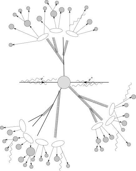
Figure 1: Scetch of an $e^{+}e^{-}$–annihilation into jets. The wiggly lines represent the photons of the initial state radiation, the thick shaded blob stands for the hard subprocess, here the production of three jets. The secondary parton radiation accounts for the inner–jet evolution, whereas the fragmentation is indicated by the ellipses with further hadronic decays indicated.

In this section, we would like to summarize the physics encoded in the new event generator APACIC++ . In its present state, APACIC++ is capable to describe $e^{+}e^{-}$ initiated processes at LEP energies and beyond putting a strong emphasis on strong interacting final states. Such processes, e. g. $e^{+}e^{-}\to$ jets, can be modelled in terms of the following steps, see Fig. 1 for comparison :

1. Initially, two beam particles, i. e. the electron positron pair, are approaching each other, usually head–on–head. Eventually they radiate photons, which are predominantly soft and collinear. Thus, as a first approximation, this initial state radiation of photons off the electrons merely changes the energies, but not the direction of the beam particles.

2. With a c. m.–energy, which is reduced accordingly, the electron positron pair interacts producing varying numbers of primary partons. The main properties of this hard subprocess and the kinematical distribution of the primary partons determine the overall features of the event. Therefore it is reasonable to concentrate in this step on final state particles with comparably high energies and large relative angles, i. e. jets.

3. The jets produced in the hard subprocess experience an evolution from the hard scales of their production down to the relatively soft scales of hadronization. In the progress of their evolution, the partons loose their timelike virtual mass via multiple splitting into pairs of secondary partons where each of the decay products is also provided with – lower – virtual masses and might decay further. This parton shower stops at some minimal virtual mass $q_{0}^{2}$ of the order of a few $\Lambda_{\rm QCD}$.

4. The resulting parton ensemble is now fragmented into the observable colour–neutral hadrons. Since this is an essentially non–perturbative process, there is a definite lack of quantitative understanding starting from first principles. Thus, parameter dependent phenomenological models have to be employed for the description of hadronization.

   However, many of the produced hadrons are unstable and decay further.

In this context, a comment is in order. As a matter of fact, the parameters of the hadronization model employed depend strongly on the energy scale related to the onset of fragmentation. In this sense, the two basic reasons for the implementation of the parton shower in event generation are

1. to give a better description of inner–jet features, and

2. to provide the hadronization model with an universal energy scale $q_{0}^{2}$ for its onset, which is independent of the c. m.–energy of the process.

In this sense, the parton shower guarantees the universality of the hadronization model.

One of the long–standing obstacles of event generation for high–energy processes is to combine the matrix elements describing the hard process of jet production to the parton shower. In APACIC++ a new algorithm was developped and implemented resolving this problem.

Apparently, the steps outlined above follow some remnant idea of time ordering and, in addition, they are characterized by roughly disjunct energy regimes. Note, that for the sake of compact expressions, here and in the following we denote by partons indiscriminately any elementary particle, i. e. leptons and the electroweak gauge bosons in addition to the quarks and gluons.

In the rest of this section, we will discuss the stages of an event named above in a slightly rearranged way. Since most of the physics features encoded in APACIC++ are already covered in a very detailled manner in various publications and textbooks[13], we will restrict ourselves to quite a scetchy presentation of these issues and corresponding references. On the other hand, the new approach for the combination of matrix elements and parton showers represents original work and therefore more care is spent on the discussion of this part.

2.1 Matrix elements

We start our tour de force through the physics encoded within APACIC++ with a discussion of the hard underlying process. Here, differences of APACIC++ to other frequently used event generators, like Pythia or Herwig become most apparent. Going beyond single exclusive channels, these generators usually start with $e^{+}e^{-}\to q\bar{q}$, populating the phase space for particle emission with help of the suitably corrected and set-up parton shower, see Subsec. 2.4.

In contrast, APACIC++ divides the phase space into two disjunct regions [14] by means of the notion of jets [KKS99a, KKS99b]. Popular jet measures available within APACIC++ are the Jade– [15] and the Durham–scheme [16], defining two particles to belong two different jets, if

$$\begin{array}[]{rcll}2E_{i}E_{j}(1-\cos\theta_{ij})&>&y_{\rm cut}s_{ee}\;\;\;\;\;\;(\mbox{\rm Jade})\\ 2\mbox{\rm min}\{E_{i}^{2},E_{j}^{2}\}(1-\cos\theta_{ij})&>&y_{\rm cut}s_{ee}\;\;\;\;\;\;(\mbox{\rm Durham})\,.\end{array}$$ (3)

Within APACIC++ , the user predefines an initial $y_{\rm cut}$, in the following called $y_{\rm ini}$, and the corresponding scheme. Then emissions characterized by a $y>y_{\rm ini}$ are described by means of the corresponding matrix elements squared, thus identifying the outgoing partons with jets according to the initial definition. The complementary regime of parton radiation with $y<y_{\rm ini}$ is covered by the parton shower. This division of phase space in two region is maintained in APACIC++ even for varying numbers of jets, i. e. the simultaneous generation of events in all channels accessible. Then, the selection of the final state proceeds in four steps, namely :

1. During the initialization of APACIC++ total cross sections for each channel under inspection in dependence on the jet–definition are either read in or calculated. To account for the impact of higher order corrections in QCD channels, some scale factors $\kappa_{n_{j}}$ are introduced to modify each $n_{j}$–jet cross section $\sigma_{n_{j}}$ by replacing the corresponding prefactor $\left[\alpha_{s}(s_{ee})\right]^{n_{j}-2}$ with $\left[\alpha_{s}(\kappa_{n_{j}}s_{ee})\right]^{n_{j}-2}$. Similar treatments can be found in [9, 17]. Within APACIC++ the running of $\alpha_{s}$ is taken in leading order.

2. Now, $n_{j}$–rates $R(n_{j})$ are defined. APACIC++ provides four different schemes, a “direct” one, two “rescaled” ones and a “resummed” one. Defining $\sigma_{\rm had}=\sigma_{ee\to q\bar{q}}$ and concentrating on events mediated by one intermediate photon or $Z$–boson, the direct one reads

   $$R(n_{j})^{\rm dir.} = \frac{\sigma_{n_{j}}}{\sigma_{\rm had}}\;,$$

   $$R(2)^{\rm dir.} = 1-\sum\limits_{n_{j}>2}R(n_{j})^{\rm dir.}$$ (4)

   and the two rescaled schemes are

   $$R(n_{j})^{\rm res1} = R(n_{j})^{\rm dir.}-\sum\limits_{n_{k}>n_{j}}R(n_{k})^{\rm dir.}\;,$$

   $$R(2)^{\rm res1} = 1-\sum\limits_{n_{j}>2}R(n_{j})^{\rm res1}$$ (5)

   and

   $$R(n_{j})^{\rm res2} = R(n_{j})^{\rm dir.}\prod\limits_{n_{k}>n_{j}}\left(1-R(n_{k})^{\rm res2}\right)\;,$$

   $$R(2)^{\rm res2} = 1-\sum\limits_{n_{j}>2}R(n_{j})^{\rm dir2}$$ (6)

   where the first scheme obviously treats $n_{j}+k$–jet configurations as subsets of $n_{j}$–configurations and the effect of the scale factors $\kappa_{n_{j}}$ is already included.

   In the fourth scheme, the resummed one, the matrix elements squared giving rise to the jetrates are combined with jetrates in the so–called NLL-scheme [DURHAM] relying on Sudakov form factors [18]. These Sudakov form factors have an interpretation as the probability of no observable branching between two scales, see Subsec. 2.4 and in leading logarithmic order they are given by

   $$\Delta_{q}^{\rm NLL}(Q_{\rm ini},Q) = \exp\left[\int\limits_{Q_{\rm ini}}^{Q}\,dq\Gamma_{q}(q,Q)\right]$$

   $$\Delta_{g}^{\rm NLL}(Q_{\rm ini},Q) = \exp\left[\int\limits_{Q_{\rm ini}}^{Q}\,dq\left(\Gamma_{g}(q,Q)+\Gamma_{f}(q)\right)\right]$$

   $$\Delta_{f}^{\rm NLL}(Q_{\rm ini},Q) = \frac{\left[\Delta_{q}^{\rm NLL}(Q_{\rm ini},Q)\right]^{2}}{\Delta_{g}^{\rm NLL}(Q_{\rm ini},Q)}$$ (7)

   with the NLL–splitting functions $\Gamma$ representing in the same approximation the branching probabilities for $q\to qg$, $g\to gg$ and $g\to q\bar{q}$, respectively,

   $$\Gamma_{q}(q,Q) = \frac{2C_{F}}{\pi}\frac{\alpha_{s}(q)}{q}\left(\log\frac{Q}{q}-\frac{3}{4}\right)$$

   $$\Gamma_{g}(q,Q) = \frac{2C_{A}}{\pi}\frac{\alpha_{s}(q)}{q}\left(\log\frac{Q}{q}-\frac{11}{12}\right)$$

   $$\Gamma_{f}(q,Q) = \frac{n_{f}}{3\pi}\frac{\alpha_{s}(q)}{q}$$ (8)

   Then, for example, the two–and three–jetrates read in NLL–approximation with $Q_{\rm ini}^{2}=y_{\rm ini}s_{ee}$ and $Q^{2}=s_{ee}$

   $$R_{2}(Q_{\rm ini},Q) = \left[\Delta_{q}(Q_{\rm ini},Q)\right]^{2}$$

   $$R_{3}(Q_{\rm ini},Q) = 2\left[\Delta_{q}(Q_{\rm ini},Q)\right]^{2}\int\limits_{Q_{\rm ini}}^{Q}\,dq\Gamma_{q}(q,Q)\Delta_{g}(Q_{\rm ini},q)$$ (9)

   and they are combined with the direct rates above by expanding in $\alpha_{s}$ and replace the coefficients for the corrsponding powers of $\alpha$ with the direct rate above, Eq. (2). Note that in this scheme, the various scale factors $\kappa_{s}$ are forced to be equal to 1.

   The jetrates defined above in the three schemes hold true for pure QCD final states and one intermediate photon or $Z$–boson. Including more electroweak gauge bosons with decays resulting in at least four fermions, the situation changes. Then two subsets are defined, where all channels with at least four fermions in the final state are excluded from the QCD–subset and added to the electroweak set EW. The cross section for this last set is given by the sum of all contributing channels, the cross section for the QCD set is still assumed to be $\sigma_{\rm had}$.

3. During the initializtion of the individual events, first the subset, either QCD or EW, is chosen according to the cross section. In case of QCD the number of jets is then determined via the corresponding jetrate, $R(n_{j})$ given above.

4. Having defined the number of jets of the event or its membership to the EW–set, the flavour constellation is picked according to the relative weight of its contribution to the jetrate or the electroweak subset.

APACIC++ itself provides expressions for two processes only, namely

$$e^{+}e^{-}\to q\bar{q}\;\;\mbox{\rm and}\;\;\;e^{+}e^{-}\to q\bar{q}g\,,$$ (10)

where both photon– and $Z$–exchange and quark masses can be taken into account [19]. In addition, APACIC++ includes interfaces to a number of matrix element generators allowing for a considerably larger class of processes, see Table 1. For further details on those generators we refer to the corresponding literature.

Generator	$\%$ of jets	LO/NLO	Quark masses	Comments
AMEGIC++ [12]	$\leq 5$	LO	yes	preferred choice, full SM
Debrecen[20]	$\leq 4$	NLO	no	QCD only
	$\leq 5$	LO	no
Excalibur [21]	$=4$	LO	no	full SM, no Higgs.

Table 1: Matrix element generators to be interfaced with APACIC++ .

2.2 Initial state radiation

Running APACIC++ with AMEGIC++ or the built–in matrix elements, there is an option to include the effect of initial state radiation of photons off the electrons. Presently, both programs allow only for quite a simple approximation in the description of this effect, namely the structure function approach [22]. In this approach, the photons are emitted on–shell strictly collinear, i. e. parallel to the beam axis and thus, they merely reduce the energy of he incoming electron. With $x$ the energy of the electron in units of its beam energy and $m_{e}$ the electron mass, the structure function has the form

$$\Phi(x) = \frac{\exp\left(-\beta_{E}\gamma_{E}+\frac{3}{8}\beta_{S}\right)}{\Gamma\left(1+\frac{1}{2}\beta_{\rm exp}\right)}\beta(1-x)^{\beta_{\rm exp}/2-1}-\frac{1}{4}\beta_{H}(1+x)+O(\alpha^{2})\,,$$ (11)

where $\beta_{\rm exp}=\beta$ and the two other $\beta_{i}$ encountered are either $\beta$ or $\eta$,

$$\beta = \frac{2\alpha}{\pi}(L-1)\;,\;\;\eta=\frac{2\alpha}{L}\;,\;\;L=\log\frac{s_{ee}}{m_{e}^{2}}\,,$$ (12)

each choice representing a different parametrization. Within APACIC++ and AMEGIC++ , this structure function $\Phi(x)$ is encoded up to third order in $\alpha$, the default setting is the so–called $\beta$–choice,

$$\beta_{\rm exp}=\beta_{H}=\beta_{S}=\beta$$ (13)

and $\Phi$ up to $\alpha^{2}$.

Including the effect of initial state radiation in this framework merely adds two more variables to the phase space integral to be performed, namely the energy fraction $x_{1,2}$ of the electron and the positron, respectively, but it does not alter the way, the jet constellation of the events is determined.

2.3 Combining matrix elements and parton showers

Following APACIC++ in the process of event generation, we turn now to the issue of combining the matrix elements described above, see Subsec. 2.1, with the subsequent parton shower to be adressed later in 2.4. Assuming LO matrix elements for jet production only, the new algorithm covering this task proceeds in the following steps [11]:

1. Having chosen the number of jets and the flavour constellation in the fashion already described above, the kinematical constellation is determined according to the corresponding matrix element with a hit–or–miss method. For this purpose one needs some maximal value limiting it from above. This maximum has already been found during the Monte–Carlo evaluation of the cross sections, which sampled the matrix element over the available phase space, and it has been stored.

2. APACIC++ provides three different schemes off additional weights multiplying the numerator of the hit–or–miss method. They are introduced to model some of the higher order effects on top of the LO matrix element. The first scheme is a direct one, which does not alter at all the distributions given by the matrix element, the second one includes the effect of running $\alpha_{s}$

   $$w^{\rm dir.}(n_{j}) = 1\;,$$ (14)

   $$w^{\alpha_{s}}(n_{j}) = \left[\frac{\alpha_{s}(y_{\rm min}s_{ee})}{\alpha_{s}(y_{\rm ini}s_{ee})}\right]^{n_{j}-2}$$ (15)

   with $y_{\rm min}=\mbox{\rm min}_{i,j}\{y_{ij}\}$, the minimum of all values $y$ between two jets $i$ and $j$ of the event and $y_{\rm ini}$ the $y$ used for the initial jet definition.

   The third scheme is the most involved one and employs additionally Sudakov form factors in the NLL–approximation, see Subsec. 2.1. Their interplay depends in a non–trivial way on the event structure and the resulting weight again resums in NLL–approximation the effect of multiple soft and collinear emissions of secondary partons.

   More specifically, this last weight is constructed recursively. Starting from a $n_{j}$–jet configuration with $n_{j}$ four momenta, the two momenta $i$ and $j$ with the smallest $y_{ij}$ are clustered yielding a new four momentum related to some internal line. The clustering is repeated until only two internal quark lines remain. Then, each internal line is weighted with a ratio of Sudakov form factors, representing the probability that no emission resolvable at the scale associated with the initial jet definition, $y_{\rm ini}$, takes place between the upper and lower scales of the line, which are defined via the corresponding values $y^{u,l}$. Outgoing lines in contrast yield merely a single Sudakov form factor with the upper scale given by the $y^{u}$ of their production and the lower scale $y_{\rm ini}$. As an illustrative example, consider the three jet configuration displayed in Fig. 2

   

   Figure 2: Typical three–jet configuration.

   with the corresponding “resummed” weight

   $$w^{\rm res}=\frac{\alpha_{s}(q^{2})}{\alpha_{s}(Q_{\rm ini}^{2})}\Delta_{q}(Q_{\rm ini},Q)\frac{\Delta_{q}(Q_{\rm ini},Q)}{\Delta_{q}(Q_{\rm ini},q)}\Delta_{q}(Q_{\rm ini},q)\Delta_{g}(Q_{\rm ini},q)\,,$$ (16)

   where

   $$Q=\sqrt{s_{ee}}\;,\;\;q=\sqrt{\mbox{\rm min}\{y_{qg},y_{\bar{q}g}\}s_{ee}}\;,\;\;Q_{\rm ini}=\sqrt{y_{\rm ini}s_{ee}}\,.$$ (17)

   For more details on this scheme, we refer the reader to [23]. There a proof is also given, that when initializing physically meaningful jetrates at $y_{\rm ini}$ this algorithm reproduces the jetrates at arbitrary larger values of the resolution parameter $y_{\rm cut}$ in leading logarithmic approximation.

3. Having determined the proper kinematical configuration in one of the three schemes introduced above, the colour constellation of the event is chosen. This is accomplished by defining relative probabilites for each parton history representing a specific colour flow. APACIC++ provides four schemes, the first two employing – if available – the Feynman–amplitudes related to the diagrams. Here, up to some appropriate normalization, the relative probabilities $P_{i}$ for each specific colour history $i$ related to some colour flow as given in a diagram/amplitude $M_{i}$ reads

   $$P_{i}^{\rm dir.1}\sim\left|M_{i}^{2}\right|\;\;\mbox{\rm or}\;\;P_{i}^{\rm dir.2}\sim\left|M_{i}\sum\limits_{j}M_{j}^{*}\right|\;,$$ (18)

   respectively.

   The third scheme employs the language of the parton shower in a fashion similar to the one presented in [24]. Here, all possible ways to reach the given configuration via a chain of $1\to 2$–branchings is constructed recursively. Each internal line contributes a factor $1/t$, where $t$ is the invariant mass of the line, and each splitting $a\to bc$ is represented by the corresponding splitting function $P_{a\to bc}(z)$. Note, that since all four momenta of the final state are known, the kinematical parameters $t$ and $z$ can easily be determined. As an illustrative example, consider the four–jet configuration depicted in Fig. 3. The relative probability in this scheme reads

   $$P = \frac{1}{t_{1}}P_{q\to gq}(z_{1\to 34})\frac{1}{t_{3}}P_{g\to gg}(z_{3\to 56})\;,$$

   $$t_{1} = p_{1}^{2}=(p_{4}+p_{5}+p_{6})^{2}\;,\;\;z_{1\to 34}=\frac{E_{3}}{E_{1}}\;,$$

   $$t_{4} = p_{4}^{2}=(p_{5}+p_{6})^{2}\;,\;\;z_{4\to 56}=\frac{E_{5}}{E_{4}}\,.$$ (19)

   

   Figure 3: Typical four–jet configuration.

   The fourth scheme applies only, if the kinematical configuration has been chosen in the resummed algorithm including the Sudakov form factors, described above. Then the colour configuration is determined as the one yielding the most advantageous clustering.

4. The final step is to provide timelike virtual masses to the outgoing partons, which so far have been on their mass shell. This is accomplished with the regular parton shower algorithm described below. The corresponding upper scales for each parton are then given by the virtual mass related to the splitting before, i. e. $t_{4}$ for partons $5$ and $6$, $t_{1}$ for parton $3$ and $Q^{2}$ for parton $2$ in the exemplary graph above. Since the subsequent parton shower is limited to model the inner–jet evolution, in the determination of the lower scale a veto is applied on unwanted virtual masses producing an additional jet, i. e. on virtual masses which translate in scales larger than $y_{\rm ini}$.

   To guarantee local four momentum conservation when providing virtual masses, the corresponding four momenta are slightly reshuffled. In close analogy to the algorithm within the parton shower, the new momenta $p_{b,c}^{\rm cor.}$ in terms of the original ones $p_{b,c}^{(0)}$ read

   $$p_{b,c}^{\rm cor.}=p_{b,c}^{(0)}\pm\left(r_{c}p_{c}^{(0)}-r_{b}p_{b}^{(0)}\right)\,,$$ (20)

   where the offsprings $b$ and $c$ stem from the internal line $a$. The factors $r_{b,c}$ are then given by

   • Case 1: b is an internal line, c is outgoing.

     $$r_{b} = \frac{t_{a}+(t_{c}-t_{b})-\lambda}{2t_{a}}$$

     $$r_{c} = \frac{t_{b}(t_{b}-t_{c}+\lambda)-t_{a}(t_{a}-t_{c}-\lambda)}{2t_{a}(t_{b}-t_{a})}$$ (21)

   • Case 2: b and c are outgoing.

     $$r_{b,c} = \frac{t_{a}\pm(t_{c}-t_{b})-\lambda}{2t_{a}}$$ (22)

   $\lambda$ is

   $$\lambda=\sqrt{(t_{a}-t_{b}-t_{c})^{2}-4t_{b}t_{c}}\,.$$ (23)

This closes the presentation of the new algorithm to combine matrix elements and parton showers as provided in APACIC++ and we turn our attention to the subsequent parton shower modelling the inner–jet final state radiation.

2.4 Final state radiation : The parton shower

The common approach to model the pattern of multiple emissions of partons constituting the final state radiation is the parton shower picture [13]. Basically, it involves the concentration on the soft and collinear regime of phase space housing the largest contributions and thus the bulk of emissions. Expanding each individual parton splitting around the corresponding soft and collinear limits results in a factorization of the full – presumably complicated – radiation structure into a chain of independent decays, which can be treated in a probabilistic manner. In this framework, the leading logarithms are resummed in two different schemes employing different order parameters, namely the ordering by virtual masses in the leading log–scheme (LLA), which is inspired by the well–known DGLAP–equation [25] , and the ordering by angles in the modified leading log–scheme (MLLA) [26]. The important effect of coherence [26, 27] in the parton shower is provided in the first scheme by an appropriate veto on rising opening angles in subsequent parton splittings [28, 29], in the second scheme this effect is incorporated in a natural fashion.

The parton shower in both schemes is organized by means of Sudakov form factors [18]

$$\Delta_{a\to bc}(t_{0}(a),t)\equiv\exp\left[-\int\limits_{t_{0}(a)}^{t}\,\frac{dt^{\prime}}{t^{\prime}}\int\limits_{z_{1}(t^{\prime})}^{z_{2}(t^{\prime})}\,dz\frac{\alpha_{s}(p_{\perp}(z,t^{\prime}))}{2\pi}\,P_{a\to bc}(z)\right]\,,$$ (24)

where $P_{a\to bc}$ is the splitting function related to the decay $a\to bc$. Eq. (24) yields the probability, that no resolvable branching $a\to bc$ occurs between the scales $t$ and $t_{0}(a)$, which is usually taken as the infrared cut–off of the parton shower. Consequently, ratios $\Delta(t_{0},t_{1})/\Delta(t_{0},t_{2})$ are identified as the probability that no branching resolvable at the infrared scale $t_{0}$ happens between $t_{1}$ and $t_{2}$. Within event generators such ratios are constructed and compared with random numbers and determine the – decreasing – sequence of scales in accordance with the ordering schemes named above.

In terms of the Sudakov form factors, LLA and MLLA differ in the interpretation of the scale parameter $t^{\prime}$. In LLA $t^{\prime}$ is the timelike virtual mass of the decaying parton, whereas in the MLLA, $t^{\prime}=E_{a}^{2}\theta_{a\to bc}$, the scaled opening angle. Consequently LLA and MLLA differ in the definition of the relative transversal momentum identified with the scale of $\alpha_{s}$ and the boundary conditions for $z$.

$$p^{2}_{\perp} \stackrel{{\scriptstyle\rm LLA}}{{\Longrightarrow}} z(1-z)t^{\prime}\stackrel{{\scriptstyle\rm MLLA}}{{\Longrightarrow}}z^{2}(1-z)^{2}t^{\prime}$$

$$z_{1,2}^{\rm LLA} = \frac{1}{2}\pm\frac{1}{2}\sqrt{1-\frac{4t_{0}(a\to bc)}{t^{\prime}}}$$

$$\sqrt{\frac{q^{2}_{0}}{t}}\leq z^{\rm MLLA} \leq 1-\sqrt{\frac{q^{2}_{0}}{t^{\prime}}}\;.$$ (25)

In APACIC++ , both ordering schemes for the parton shower are available, the additional angular veto in the LLA–scheme can be switched off by the user. Note, that within APACIC++ the first splitting of a parton within the shower is always performed in the LLA–scheme. This is due to the fact, that by construction MLLA is only applicable in the region of small angles, which might not yet be reached for the first branching.

However, in APACIC++ running with the LLA–scheme each parton leaves the parton shower with a flavour dependent virtual mass,

$$t_{0}(f) = \mbox{\rm min}\{q_{0}^{2},m_{f}^{2}\}\;,$$ (26)

thus restricting the minimal virtual mass for each specific decay channel via

$$4t_{0}(a\to bc) = \left[\sqrt{t_{0}(b)}+\sqrt{t_{0}(c)}\right]^{2}\,.$$ (27)

This results in restrictions $4t_{0}(g\to bb)\geq 4m_{b}^{2}$ for gluons splitting into two $b$–quarks and $4t_{0}(b\to bg)\geq(m_{b}+q_{0})^{2}$ for decays $b\to bg$. Therefore, within APACIC++ the Sudakov form factors are constructed as the sum of form factors corresponding to the individual possible decays. In the algorithm of APACIC++ individual splittings proceed as follows

1. Starting with the upper scale $t_{1}$ first the virtual mass of the next observable decay of parton $a$, $t_{2}$ is determined via the comparison of a random number $\#R$ with the appropriate sum of Sudakov form factors,

   $$\#R\stackrel{{\scriptstyle!}}{{=}}\frac{\sum_{bc}\Delta_{a\to bc}[t_{0}(a\to bc),t_{1}]}{\Delta[t_{0}(a\to bc),t_{2}]}\Longrightarrow t_{2}.$$ (28)

2. Then the energy fraction $z^{\prime}$ is determined according to the sum of splitting functions with a hit–or–miss method. Here, first a $z^{\prime}$ is chosen uniformly in the maximal allowed range of all decay channels,

   $$\mbox{\rm min}\{z_{1}(a\to bc)\}\leq z^{\prime}\leq\mbox{\rm max}\{z_{2}(a\to bc)\}$$ (29)

   Then, a random number is compared with the ratio of sums of splitting functions taken at $z^{\prime}$ and their specific maximal value.

   $$\#R\stackrel{{\scriptstyle?}}{{>}}\frac{\sum\limits_{bc}P_{a\to bc}(z^{\prime})}{\sum\limits_{bc}P_{a\to bc}^{\rm max}}\,,$$ (30)

   where the $z^{\prime}$ is accepted or rejected if the random number is larger or smaller than the ratio.

3. Having determined the decay kinematics by the $t^{\prime}$, $z^{\prime}$ the flavours of the outgoing partons are selected according to the relative weight of the corresponding splitting functions at $z^{\prime}$.

4. The outgoing partons are equipped with virtual masses themselves, starting from $t_{a}$. For each combination, Eqs. (20) and (22) are applied to guarantee local four momentum conservation. If no combination of appropriate $t_{b}$ and $t_{c}$ can be found respecting $t_{i}\geq t_{0}(i)$ and keeping $z^{\prime}$ and the opening angle $\theta_{a\to bc}$ in the allowed region, APACIC++ returns to step 1 of this algorithm.

5. The final task to be completed is to assign an azimuthal orientation to the decay plane with respect to the previous one. APACIC++ provides two options, namely

   • the uniform distribution of the relative angle $\phi$, or

   • the inclusion of azimuthal correlations, [30],

   which can be chosen by the user.

2.5 Fragmentation

After the parton shower has terminated at the cut-off virtuality $q_{0}^{2}$ the domain of long-distance interactions characterized by comparably low momentum transfer is reached. At this point QCD turns strong–interacting and non-perturbative effects take over their reign, converting the partons of perturbative QCD into the observable hadrons, a process which is called either fragmentation or hadronization. Since it is non–perturbative any traditional method of perturbative field theory meets with disaster and there is no approach derived from first principles to describe this process on a quantitative level. Consequently, the only way out is the construction of phenomenological models.

Currently, APACIC++ uses the fragmentation model provided by Pythia, namely the Lund String–model [31]. Historically, the string hadronization scheme [32, 33] was introduced as an alternative to the independent jet fragmentation scheme. The independent fragmentation scheme is the simplest and oldest model for translating partons into hadrons and was developped by Field and Feynman [34]. Here, the hadronization of a $q\bar{q}$ pair is a recursive process starting with the generation of a secondary $q_{1}\bar{q}_{1}$ pair out of the vacuum. Then, the $q$ and $\bar{q}_{1}$ are combined into a meson. The procedure is iterated starting from the $\bar{q}q_{1}$ pair until the remaining energy of the corresponding left–overs falls below a cut-off. The production of the secondary quark pairs is modelled by the so–called fragmentation functions, yielding the probability distribution for a quark flavour $q$ to turn into a meson $M$ depending on the energy fraction $z=E_{M}/E_{q}$. Selecting the type of $M$ the flavour of the antiquark and thus the flavour and the remaining energy of the secondary quark pair is determined. In the independent fragmentation approach these functions are scale independent. The hadronization of a gluon can be incooperated by splitting the gluon into a $q\bar{q}$ pair. However, a shortcoming of the independent fragmentation scheme is, that the partons are treated on–shell. This leads to a violation of four–momentum conservation, which has to be cured by rescaling the kinematics of the hadron ensemble, once the hadronization process has terminated.

In the string concept the $q\bar{q}$ pair is not independent any more but strongly correlated by a one-dimensional classical object, the string. The string plays the role of the stretching colour field between the quarks and produces a potential between them which increases linearly with their distance. The simplest $q\bar{q}$ configuration leads to the so-called yo-yo string and its classical evolution would result in an oscillation of the bound quark-antiquark pair. However, within a relativistic quantum mechanical system the energy can condense into the production of a flavour neutral $q_{1}\bar{q}_{1}$ pair which screens the chromoelectric field. The resulting ensemble thus decouples into the two color neutral systems ($q\bar{q}_{1}$ and $q_{1}\bar{q}$), where each of them is subject to further dissociations into smaller systems. So, hadronization is modelled as the break–up of a string in smaller ones, where each string hosts a $q_{i}\bar{q}_{j}$–pair at its endpoints, which eventually are transformed into mesons or their resonances. Since the break–up of the strings into smaller ones is mediated by the production of a secondary $q\bar{q}$ pair, the fragmentation functions encountered before come into play again, although in a slightly modified form. In the Lund picture, the string break–up is interpreted in terms of tunneling phenomena, heavy masses are suppressed for the secondary quarks with ratios of roughly $u\bar{u}:d\bar{d}:s\bar{s}:c\bar{c}\approx 1:1:0.3:10^{-11}$. Additionally, the transverse momenta of the primary hadrons coming into existence are chosen according to a Gaussian distribution with the width $\sigma_{q}$. This width is one major parameter of the hadronization, which has to be adjusted. The Lund fragmentation function reads

$$f(z)=z^{-1}(1-z)^{a}\exp{(-bm^{2}_{\perp}/z)}\,,$$ (31)

with $m_{\perp}$ the common transverse mass of the secondary $q\bar{q}$ pair determining the tunneling probability. Furthermore, the Lund fragmentation function is left–right symmetric, i. e. the results are independent on the choice of the starting point for the break–ups, quark or antiquark. Basically, the parameter $a$ could be flavour–dependent, while the parameter $b$ is not. However, phenomenologically there is no need to introduce different $a$’s. Thus the Lund fragmentation function has two parameters $a$ and $b$, which form the set of three major hadronization parameters to be set by the user in the file parameter.dat.

Again, in the simplest realization of the string model, the quark–antiquark pairs are transformed into mesons or their resonances with matching masses. More involved schemes like the Lund string allow for the incorporation of baryons, too. For more details we refer the reader to the literature. However, the hadrons themselves experience further decays of various types resulting in an ensemble with long–lived hadrons.

In the string model gluons are incorporated as “kinks” on the string carrying finite energy and momentum. Rephrased in other words, unlike the quarks the gluons are attached to two string pieces and thus their fragmentation is different from that of the quarks. Addionally, the kinks on the string also modify the dynamics. Hence, the one-dimensional yo-yo type description of the motion is not valid any more. Fortunately, covariant evolution equations for kinky strings also exist.

The string approach to hadronization has several advantages over the independent jet model. The basic assumptions of the string model seem to be in better agreement with the general ideas of QCD, on the lattice for example, “flux tubes” in quite a close analogy to the string have been found. Furthermore, in the string model energy, momentum and flavour are conserved at each step of the fragmentation process, because at each iteration (break–up) the whole system is considered. Last but not least, the results of Monte Carlo simulations are in far better agreement with experimental data.

3 Program Structure

In this section, we will discuss in some detail how the physics features outlined above manifest themselves in the program APACIC++ . We refer those of the users not interested in any internal details directly to Sec. 4, where we list necessary prerequisites and steps to install and run APACIC++ .

However, since this program consists of roughly 8000 lines organized in 74 classes contained in the C–files plus slightly more than 2000 lines in the corresponding header files, and because there are quite strong connections to the even larger program AMEGIC++ , the description necessarily has some shortcuts. Nevertheless we hope, that the following subsections will provide any potential reader a sufficient background for understanding the code. We start our presentation in Subsec. 3.1 with a brief introduction into the basic strategies underlying APACIC++ and the essential structures for their implementation. In Subsec. 3.2 we describe, how APACIC++ generates event samples and individual events. The next part, Subsec. 3.3, is devoted to a discussion of the handling of the matrix elements, before we turn to the implementation of the parton shower in Subsec. 3.4. Finally, the issue of fragmentation within APACIC++ will be covered in Subsec. 3.5.

3.1 Basic strategies and structures

In principle, APACIC++ has its main focus on simulating the whole parton level of an event. Starting from the incoming beam particles, currently constrained to be an $e^{+}e^{-}$ pair, initial state radiation, hard scattering processes and the subsequent parton shower is covered. Then, after translating the parton ensemble appropriately into the HEPEVT–block, some hadronization scheme is invoked, which at the moment is the Lund–string implemented in Pythia. Consequently, the bulk of algorithms within APACIC++ deals with the simulation of events on the parton level, the hadron level is covered via the corresponding interface. Hence, our desciption of the basic strategies will focus on the parton level.

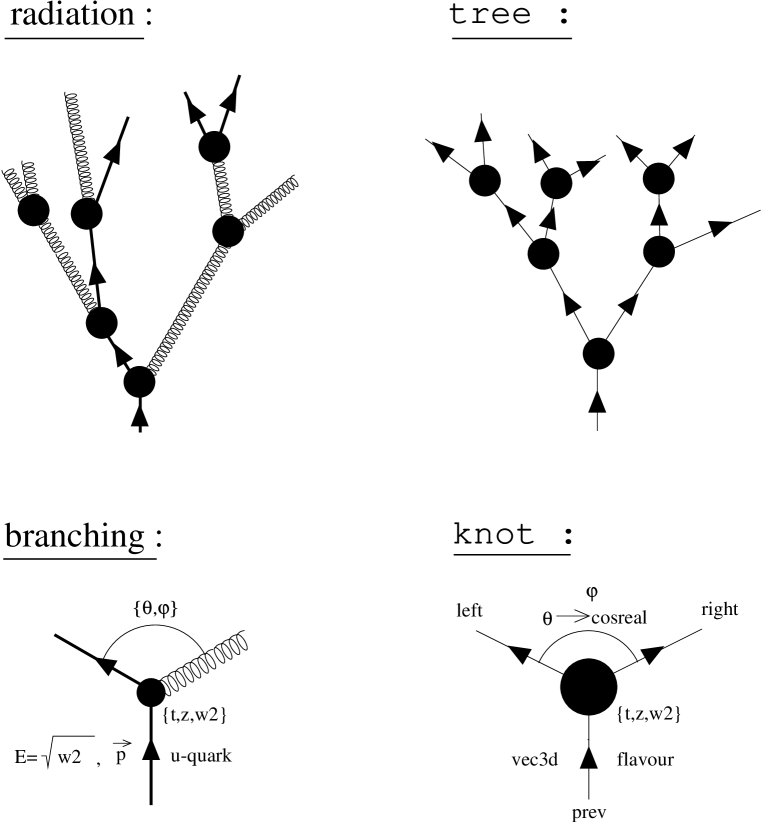
Figure 4: Scetch of the mapping between radiation processes and the corresponding classes. The full radiation pattern is identified as a chain of $1\to 2$ processes, a Markhov chain, which translates into the class tree. The basic building blocks, the binary decays, in turn are realized with knots. Thus a tree contains a list of linked knots.

The first observation underlying simulations in particle physics is, that the objects to be dealt with appear in two different contexts. First, the particles can be classified according to their properties, i. e. charges, masses and the like. In APACIC++ this information is contained primarily in the class flavour, supplementing methods to define anti–particles or the link between different numbering schemes for the particles. In contrast, the individual particles with their properties defined in flavour have to be tracked through a single event. The paradigma underlying APACIC++ is to

define and treat partons within the event structure via their decays.

More specifically, the partons are dealt with by means of their $1\to 2$–decays. This is motivated by the following two observations:

1. In the language of the leading logarithmic approximation, the radiation pattern of an event on the parton level reduces to a series of subsequent binary branchings, a Markhov–chain. Therefore, the basic building blocks of the parton shower can be identified easily with such $1\to 2$ decays, outgoing partons in this framework can be treated via “non–existing” $1\to 2$ decays.

2. Usually, the vertices encountered have either three or four external legs. However, within the Standard Model and its simpler extensions, the vertices with four legs can always be decomposed into the product of two vertices with three legs and one propagator in between. In fact, this is the strategy employed within AMEGIC++ .

Thus, the full radiation pattern of an event translates into a Markhov–chain of subsequent $1\to 2$ branchings, see Fig. 4. This binary structure is recursive, since branchings follow each other. It is realized within the class tree, which technically contains a list of linked knots mirroring the basic building blocks, the branchings. The knots harbour links to the previous, the right and the left ones, allowing to climb up or down the tree by just following the pointers. In this framework partons entering fragmentation do obviously not experience any further decay and thus such “dead ends” are identified with knots with empty outgoing lines, i. e. empty right– and left–pointers. To dwell a little longer on this issue, we would like to confront the branchings and the knots with each other. The branchings, for instance, are specified via :

1. The three flavours, the incoming and the two outgoing ones, which in turn are incoming for the next splitting. The flavours define the splitting function of the decay, responsible for the $z$–spectrum of the decay.

2. The kinematical variables related to the decay, namely the virtual mass of the incoming particle, $t$ (or the $t=\theta E^{2}$–scale in MLLA), the energy fractions $z$ and $1-z$ of the two decay products and the azimuthal angle $\phi$. Together with the Energy $E$ and the three–momentum $\vec{p}$ of the decaying particle, the kinematics are fixed. For the inclusion of angular ordering “by hand”, the opening angle $\theta$ then has to be compared with the previous one, $\theta_{\rm crit}$.

The knots in full analogy include information about

1. the predecessor and the two subsequent knots via pointers pref, right and left, respectively, as well as the incoming flavour,

2. the kinematical parameters list above, namely t, ts, z, w2$=E^{2}$, cosreal$=\cos\theta$, crittheta$=\theta_{\rm crit}$ and $\phi$.

Therefore, for their proper treatment within APACIC++ , the final states stemming from the hard subprocess are translated into chains of subsequent $1\to 2$ decays, see Fig. 5, before they experience their evolution down to the scales of fragmentation. This is done with the help of the methods provided in the virtual class xsee and their derivatives, providing interfaces to the various matrix element generators. They in turn are organized as a list within xsec. In this context, we would like to stress, that the fragmentation scheme of Pythia demands some specific information of the colour structure of an event. This is best formulated in some language relying on the parton shower approach incorporating the leading logarithmic approximation for multiple emission, too. Thus, already the final states produced by the matrix elements are translated into the tree–structure, independent of whether the subsequent parton shower models the jet–evolution or not.

Figure 5: Scetch of the mapping between the hard cross sections as provided within xsec and the further treatment of the final state via tree. The translating class xsee includes their derivatives, too. In fact these derivatives contain the interfaces to the matrix element generators yielding the cross sections. The interfaces are organized as a list within xsec.

Additional classes are frequently employed by other parts of the program. However, in most cases they are highly self–explanatory and therefore do not demand any detailed discussion. They include vec3d, vec4d, jetfinder, etc.. The class random contains different random number generators, see [35]. Out of this group we would merely like to highlight some of the features of the class analyse doing the event analysis. analyse provides histogramms for some observables, namely

1. multiplicity,

2. thrust, $C$– and $D$–parameter, sphericity, aplanarity and rapidity with respect to the thrust–axis,

3. $p_{\perp}^{\rm in}$ and $p_{\perp}^{\rm out}$,

4. jet–broadening,

5. $y_{5\to 4}$, $y_{4\to 3}$ and $y_{3\to 2}$, and

6. the four jet angles $\alpha_{34}$, $\chi_{BZ}$, $\phi_{KSW}$ and $\theta_{NR}$ [36].

Within the method init(), all of these histogramms, which are classes themselves, are initialized. There, their individual number of bins and their range is defined, too. Hence, this is the place for eventual alterations. The methods fillanevent() and drawallevents() are responsible for filling in the data into the histogramms and for giving the final output. Some summarizing remarks can be found in the files allevent.dat, other observables are to be found in corresponding .dat files.

Note, however, that three classes analyse analyze the events after the matrix elements, the parton shower and hadronization, respectively. The corresponding output can be found in the subdirectories output/me.JOBNUMBER, output/parton.JOBNUMBER, and output/hadron.JOBNUMBER. The .dat files are written out at least in steps of 10000 events.

3.2 Generating events

Figure 6: Scetch of the interplay of the fundamental classes when running APACIC++. Depicted are the two central classes of APACIC++ , apacic and cascade, together with their most important methods and how they cooperate. The communication and relationships of the two steering classes with the other main parts of APACIC++ are indicated, and the methods of the other classes responsible for the contact with apacic and cascade are shown.

For the generation of events, APACIC++ involves two central classes, namely apacic and cascade. In general terms, apacic is the steering class responsible for the generation of event–samples and houses all the methods necessary to initialize and run a given number of events and to provide links to their analysis. Also, interfaces are included to link the other two event generators available, namely jetset() and herwig(). However, we will not comment on them and focus on the running of APACIC++ . When running apacic, a loop over single events is performed within the class apacic. In this loop individual events are initialized and simulated by means of the methods contained in cascade. The hope behind this structure is, that it allows for a quick extension to other processes like e. g. proton–proton collisions, and for a transparent link to other generators.

3.2.1 Sample generation

In APACIC++ the central class responsible for the production of a sample of events and steering calls to each single event is apacic. Its formal overhead is contained in main(). Here, first apacic.init() is called reading in the files particle.dat and parameter.dat and initializing particle information like charges and masses and the set of steering parameters and switches like coupling constants and the preferred shower scheme, respectively. Then, the c. m.–energy squared, $s_{ee}$, and the number of events to be generated, $N_{ev}$ is transferred into the class apacic. Now the scene is set to chose the generator for the loop over events. APACIC++ provides interfaces to Pythia and Herwig, but in the framework of this paper we want to concentrate on event generation by means of APACIC++ .

Chosing this option, main() calls apacic.electron_positron(). In this method, specific features for event generation via APACIC++ are initialized with help of apacic.initapacic(). Translated into the class structure of APACIC++ , these include

1. the class tree steering the parton shower with the method tree.init(), see Subsecs. 2.4 and 3.4,

2. the class hadron responsible for the subsequent hadronization by means of hadron.reset(), see Subsecs. 2.5 and 3.5,

3. the class interface for the link to the corresponding Fortran programs via interface.init(), see SubSec. 3.5.2

4. the class analyse for analyzing the events, and

5. the class xsec handling the hard cross sections available with the more complicated call xsec.set_xs(create_xssum,$\dots$), see Subsecs. 2.1 and 3.3.

Now, within apacic.electron_positron() the loop over single events is performed, resulting in multiple calls of apacic.oneevent(). The handling of the single events will be covered in the following Subsubsection, 3.2.2. apacic.electron_positron() closes by calling the final analysis in apacic.endapacic().

3.2.2 Event generation with APACIC++

The method apacic.oneevent() envelopes the pre–event resetting of the classes tree and hadron responsible for the parton shower and the hadronization, respectively, and the steering method apacic.epem(). This method provides the link to the class cascade and organizes the sequence of steps supplied there for the generation of single events. In chronological order, the methods of cascade employed are:

1. cascade.epem_init() determines the jet–configuration and eventually performs the jet–evolution by calling xsec.produce(), see Subsec. 3.3. This method returns a structure knot, carrying all information about the subsequent chain of branchings. Additionally, the momenta of the first two of the outgoing particles are constructed. Their virtuality determines the distance they travel, before they decay.

2. cascade.next() : A loop over all particles is performed, where each iteration is related to some time measure. In each step cascade.branch() determines, whether the particles experience a decay or not. Note, that most of the characteristical parameters of the decays, like kinematics and decay products, are already predefined. The corresponding information is contained in the tree returned by xsec.produce() via its root–knot spanning it. After the branchings were performed, in each iteration the particles are propagated via cascade.propagate(). The loop is left, if no more branching takes place on the parton level.

3. cascade.onshell() is finally applied to set all particles on their mass–shell under the constraint of global four–momentum conservation. Thus, the parton ensemble is now prepared for hadronization. It should be noted, however, that since in the current version the Lund–string as provided by Jetset takes care of hadronization, the corresponding HEPEVT–block has to be filled in appropriately. This task is performed during each individual branch described above via the method hadron.insert().

3.3 Matrix elements

The basic ideas behind the structure to be explained in the following are

• to have only one class, xsec, communicating with the steering classes apacic and cascade,

• to define standards for interfaces to a variety of matrix element generators in some virtual class xsee,

• to organize the interfaces, i. e. cross sections, in a list, xs_sum for easy access,

• to keep any tools for the evaluation of total cross sections separate, xsee_tools.

This leads naturally to a splitting in various classes, they and their mutual communication are depicted schematically in Fig. 7.

3.3.1 Organization

Figure 7: Scetch of the interplay of classes governing the initialization, evaluation and running of cross sections for the hard subprocess.

The class xsec is the general steering class for the evaluation of matrix elements. It contains a list of interface classes in xs_sum, one for each channel under consideration. The interfaces represent the connection to the corresponding matrix element generators used and they are derived from the virtual class xsee. This class defines the minimal standard of methods, each interface, i. e. each individual matrix element, has to supplement when linked. The list of cross sections is organized by means of and contained in the class xs_sum. Only a few methods are employed within xsec:

1. set_xs handles the initialization of the matrix elements and is called from apacic.initapacic() with xscreator and the incoming flavour as arguments. Note, that the class xscreator is a virtual class and represents the mother for the two classes create_xs and create_xssum, where only the latter is relevant in the following. The sequence of this initialization is :

   1. The method xscreator.create() initializes merely an array of interface classes, each derived from xsee. This array is stored in xs_sum. The incoming flavour help to define the number of relevant channels to be initialized.

   2. The jetfinder algorithm needed for integration is initialized via the method jetfinder.setinitial().

   3. Eventually the NLL–Sudakov form factors are calculated within nll.init(). They are stored in form of a look-up table derived from the class fastfunc and evaluated, i. e. read via calling the methods nll.deltaq() and nll.deltag() for the quark and gluon Sudakov form factor respectively.

   4. The method xs_sum.init() initializes the interfaces to the matrix element generators using the array of step (a). It evaluates the total cross sections.

2. produce() determines the specific final state of the individual event and a sample of momenta distributed according to the differential matrix element plus some eventual extra weight. produce() is called by the method cascade.epem_init(). First, a specific channel is chosen according to the jetrates by calling xs_sum.set_num(). The determination of the corresponding momenta is accomplished with Monte Carlo methods according to the following procedure :

   1. The maximum of the differential cross section under consideration is obtained from the method xs_sum.maximum().

   2. A sample of momenta as well as the appropriate differential cross section is determined via calling xs_sum.partial().

   3. The additional weight for the kinematical matching is evaluated according to the different options, where no weight at all, the $\alpha_{s}$ or the Sudakov weight are at disposal. The latter is calculated with the method xsec.nllfactor().

   4. The product of the extra weight and the differential cross section over the total maximum is compared with a random number. If it is smaller the momentum sample is rejected and the procedure is repeated starting with step (b).

   5. The translation of the final state of the matrix element into the list of linked knots of the parton shower and its further evolution are performed by calling the method xs_sum.makeknots(). If this step fails, the procedure returns to point (b) as well.

   The resulting list of linked knots representing the full partonic stage of the event is returned in the form of a link to the appropriate first knot.

3. nllfactor evaluates the weight for the Sudakov kinematical matching. The pre-calculated Sudakov form factors as well as the jetfinder for the determination of the jet resolution parameter $y_{\rm cut}$, jetfinder.jet(), are prerequisites for this task and called accordingly.

3.3.2 Creating a xs_sum

The class create_xssum produces a list of cross sections stored in the class xs_sum. This class appears when different channels, i.e. different final states for the same incoming particles, are included. However, in a typical APACIC++ run this is always the case. The only method of the virtual class xscreator inheriting create_xssum is create, where the incoming flavours represent the input and the accomplished list of cross sections the output. It is called by the method xsec.set_xs(). In create_xssum.create() first, the number of channels is specified. Then, according to the number of jets and the possible outgoing flavours, channels are selected and the corresponding interface classes are added. The specific choices depend on the parameter pa.jet(), the switches connected with the selection of matrix element generators (for instance sw.amegic()) and the different models (for instance sw.QCD() to be used.

3.3.3 The list of cross sections, xs_sum

The class xs_sum contains a list of interfaces to matrix element generators. It is responsible for all interactions with them. In our approach an interface class is always derivated from the mother class xsee, which defines the standard for implementing a new generator. Note, that for every process with fixed incoming and outgoing flavours the array includes a new interface class. The different methods of xs_sum fulfill the following tasks:

1. init() is used for the determination of the total cross sections and responsible for their proper normalization. It is called by xsec.set_xs(). First, the different interface classes will be initialized via xsee_tools.init(). The calculation of the total section as well as the determination of the maximum of the differential cross section are the tasks of this method. Then, the cross sections have to be normalized via normalize() to the appropriate inclusive $2\to 2$ process, for instance in the framework of QCD to $\sigma_{0}(e^{+}\,e^{-}\to q\bar{q})$. Now, the derived jetrates for different numbers of jets must be combined, which is not a unique task. Three different schemes are at disposal, which are implemented in the method rescale(). One option then is to use resummed rates, which is achieved in the method NLLmatch().

2. normalize() accounts for the proper normalization of the jetrates. The total cross sections for two outgoing particles are collected depending on the outgoing quark flavour. Accordingly every cross section is normalized to the appropriate inclusive twojet rate.

3. rescale() : The different schemes for combining jetrates with different numbers of jets are implemented in this method. Details can be found in the physics write-up, Eqs. (2),(2) and (2).

4. NLLmatch() calculates the resummed jetrates and matches them to the direct jetrates. First, for every number of jets the appropriate rate has to be determined. Then the resummed as well as the matched rate are determined with the method nll.calculate(). Finally, the different jetrates are rescaled according to the matched rate. Now, the twojet rate can be evaluated as one minus the sum of the multijet rates.

5. set_num() is called by the method xsec.produce() and assigns the channel for the hard subprocess of the event according to the jetrates. A marker ist set on the interface class of this channel, which is used for later evaluations with the specified cross section.

During the event generation a number of additional methods are employed. They provide links to the interface class, which has been selected and marked in the routine set_num(). Typical methods contain the setting and reading of the maximum of the differential cross section or the jetrate. In connection with the determination of a sample of momenta the methods partial() and get_ycut() are employed. They return the differential cross section and the minimal jet resolution parameter $y_{\rm cut}$ of the jet constellation, respectively. The method makeknots() is responsible for the combination of the chosen matrix element with the parton shower evolution.

3.3.4 Integration of ME’s

The integration of the matrix elements resulting in the total cross sections is governed by the class xsee_tools. The following methods are used for calculating, storing and reading in results.

1. init() is the only method called from outside this class, i.e. from the method xs_sum.init(). Its first step consists in the determination of the appropriate power of $\alpha_{s}$. This is, because inside the matrix element generators $\alpha_{s}(s)$ is used, and correspondingly a factor of $(\alpha_{s}(\kappa_{S}s)/\alpha_{s}(s))^{N_{\rm jet}-2}$ has to be multiplied to every total cross section for consistency reasons when including scalefactors $\kappa_{S}$. Note, that this procedure holds in the framework of pure QCD only. In the second step the jetfinder and the interface to the matrix element are initialized. Now the total cross section can be calculated by means of the method jetrate(), which yields the maximum of the differential cross section, too. In the last step the resulting values for the maximum and the total cross section are set in the interface class.

2. jetrate() maintains the calculation of the total cross section, which contains not only the evaluation but also the storage of the results for later use. For this purpose, first every process is equiped with an ID in set_processID(), which depends on the specific final state. Then the directory me is searched for the corresponding file. In case it is found, a simple read–in by means of the method input() finishes this routine. Otherwise the method calculation() determines the total cross section as well as the maximum of the differential cross section. Finally, both are stored in a table with the corresponding values in dependence on the jet resolution parameter $y_{\rm cut}$.

3. calculation() handles the determination of the total cross sections employing the following steps :

   1. The look–up table for the total cross sections is initialized with the method histofunc.reset().

   2. The phase space generator is initialized via its constructor psgen(). Note, that this generator is lend from the matrix element generator AMEGIC++ . A description of the different modes, which are the integration of the matrix element with Rambo[37] and with multichannel methods[38], can be found in [12]. The corresponding method used for the generation of the phase space is given by sw.multichannel().

   3. At this stage a loop over the corresponding Monte Carlo points is performed. In every step a point in phase space together with its weight will be generated with the method psgen.partial(). Then the minimal $y$ of the four vectors is calculated with jetfinder.y_jettest(). The value of the differential cross section, obtained from xsee.partial() and multiplied with the proper weight of this phase space point is stored in the look-up table via histofunc.insert(). In case the multichannel-method was chosen the loop ends with an optimization step in psgen.optimate().

   4. Finally, the look-up table is stored by means of the method histofunc.output().

3.3.5 Interfaces

Figure 8: Scetch of the various interface classes available within APACIC++ for the connection to the matrix element generators, which can be linked. Included are some of the communication lines with other classes handling cross sections, namely xsec and xsee_tools.

All interface classes are derivated from the class xsee, see Fig. 8. It defines the standards for communicating with any matrix element generator used. The class is purely virtual, i.e. it has no genuine method. However, since most of the methods in all interfaces have the same purpose, they are described at this stage.

1. partial() determines a sample of momenta, the appropriate weight in phase space and the differential cross section. Performing these tasks the methods of the considered matrix element generator are used. The mininal jet resolution parameter is determined by the method jetfinder.y_jettest() and accessed via get_ycut(). partial() is used by the method xsec.produce() and returns the differential cross section multiplied with the phase space weight.

2. partial(vec4d) in contrast returns the differential cross section for a given sample of momenta, which is represented as a list of 4-vectors (vec4d). It is called by the method xsee_tools.partial().

3. calculation() : A calculation of the total cross section inside the matrix element generator is implemented only in two interfaces. The reasons are in the first case, that a Next-to-Leading order calculation is performed (DEBRECEN) and in the second case, that a multichannel approach during the integration is used (EXCALIBUR). Obviously, in both cases specific features of the corresponding calculation or method had to be encoded. In the latter case an additional issue to be dealt with was transformation of the momenta into the internal structure. When necessary, this routine is called from xsee_tools.jetrate() instead of the generell integration routine xsee_tools.calculation().

4. makeknots() : The combination of the matrix elements and the parton shower strongly depends on the generator under consideration and its internal structure. Consequently, a non–general method makeknots() is needed for this task, where the different approaches of reconstructing a parton shower history are implemented, see Subsec. 2.4.

Additional methods for exchanging informations between the interfaces and the class xs_sum are provided. Most of them are self–explanatory, therefore we will not discuss them in detail. Consider as examples the methods njet(), maximum(), and integrated() yielding the number of jets, the maximum of the differential cross section and the total cross section, respectively.

Interface Class	Number	QCD	EW	Mass	Matching	Other Features
Name	of Jets				Options
xsee_apacic	2,3	X	-	X	0	none
xsee_amegic	2,3,4,5	X	X	X	0,1,2,3	+ Higgs
xsee_debrecen	3,4,5	X	-	-	0	+ NLO for 3,4 jets
xsee_excalibur	4	X	X	-	2,3	4 fermions only

Table 2: Matrix Element Generators interfaced to APACIC++

The interfaces to the four different matrix element generators, namely the internal generator of APACIC++, AMEGIC++ , DEBRECEN and EXCALIBUR, as well as some specific features are listed in table 2. As already explained in Subsec. 2.3, APACIC++ provides different options for the determination of the relative probabilities connected to the colour structure of a given final state produced by some matrix element. Therefore, within the combination procedure of matrix elements and the parton shower, these different approaches for reconstructing a parton shower history are reflected in different algorithms with corresponding methods, namely

1. The parton shower history will be reconstructed by means of the method tree.histjets(). Employing this method, the matrix element generator is not used for the determination of the relative probabilities of the different colour configurations. Instead, the probabilities are calculated in the parton shower oriented picture.

2. This option exist for the interface xsee_amegic only and is performed within the method makeknots(). AMEGIC++ constructs the Feynman amplitudes via binary trees of linked points, which is in striking analogy to the tree–structure of APACIC++ . Thus, this method merely “translates” the matrix element–points, which include all kinematical information needed, into the linked knots of tree. Consequently, the calculation of the parton shower probability like the one encountered in Eq. (3) is straightforward.

3. The probability of a parton history is proportional to the appropriate matrix element squared, see the first of Eqs. (18). Hence, it has to be calculated with the matrix element generator used.

4. When including interference effects between the different matrix elements in the spirit of the second of Eqs. (18), the probability has to be evaluated inside the matrix element generator, too.

Every interface class contains some specific methods beyond the standard methods defined within the virtual mother class xsee. These additional methods are neccessary for the appropriate connection to the matrix element generator. Furthermore, every class provides a different implementation of the method makeknots() in accordance with the different options used for the determination of the relative probabilities highlighted above. In the following, we briefly outline the additional methods, and we comment on the details related with makeknots for each of the interface classes.

1. xsee_apacic : Since all methods for the calculation of the cross sections are contained within the interface class itself, the tasks and methods are :

   1. The calculation of the differential cross sections in twojet() and threejet() for the processes $e^{+}\,e^{-}\to q\bar{q}$ and $e^{+}\,e^{-}\to qg\bar{q}$, respectively.

   2. The determination of the total cross sections in r_qq_bar(), sigmaWW() and sigmaZZ() for the electron positron annihilation into quark, $W$–boson, and $Z$–boson pairs.

   The reconstruction of the colour configuration within makeknots relies on tree.histjets().

2. xsee_amegic : Interfacing the matrix element generator AMEGIC++ all four different options for the reconstruction of the colour configurations and their relative probabilities are available. The first one corresponds to the parton shower oriented approach and employs the method tree.histjets() for the histories and their probabilities. For the three other options the probabilities of the colour configurations are determined as follows:

   1. The translation of the internal representation of the Feynman diagrams within AMEGIC++ into probabilities is performed via the method makeprob(). In recursive steps the tree of linked points is used to evaluate the parton shower oriented probability. In each point representing a $1\to 2$–vertex, the energy fraction $z$ and the virtual mass of the incoming as well as the flavours of the outgoing partons are used. The appropriate splitting function is taken into account by timebranch.set_ds() utilizing the two outgoing flavours. The value of the splitting function is calculated with (timebranch.dsp).differ(). After combining it with the virtual mass of the incoming particle, the contribution of this point to the probability is determined. The method makeprob() is called recursively with the left– and right–pointers of the structure point until the calculation terminates with the outgoing partons.

   2. The probabilities are calculated during the evaluation of the matrix elements within AMEGIC++ .

   Having at hand the probabilities for each colour configuration, one of them is choosen accordingly. In the next step eventually the linked points of AMEGIC++ are translated into the linked knots of APACIC++ . The procedure employed is the same for the last three options above. Again, the corresponding method translate() employs a recursive structure, where in every step a point is translated into a knot, the pointers to the left and the right point are translated into links for the related new knots initialized with tree.newk().

3. xsee_debrecen : Since the calculation of Next-to-Leading order cross sections involves algorithms, which are a priori not included in the integration routines contained in xsee_tools, specifc methods are neccessary for this task:

   1. jetrate() : Three different parts for the calculation of NLO cross sections must be considered. Therefore, this method can be called from the routine calculation() which leaves the evaluation of cross sections to the matrix element generator. Accordingly, three different terms, related to the born term, the loop corrections and the real corrections due to additional legs, have to be added. The distinction between these parts is shifted to subsidiary methods. However, the calculation with the typical loop over the events is performed in the usual manner. For the evaluation of the differential cross sections the method jetpartial() is employed.

   2. jetpartial() : Typically, the random construction of momenta is the first step in the calculation of a differential cross section via Monte Carlo methods. Here, difficulties arise from the different dimensions of the phase space for the different parts. Therefore the phase space for $N+1$ particles is created out of the $N$ particle phase space. After the calculation of the minimal jet resolution parameter with D_jettest() the appropriate differential cross section is determined.

   3. D_jettest() evaluates the minimal jet resolution parameter for a given sample of momenta and a pre-defined number of jets. It mirrors the methods of the class jetfinder, but with the slightly different description of 4-vectors used in Debrecen.

   4. translate() transforms a 4-vector from the APACIC++ (vec4d) to the Debrecen (LorentzVector) convention.

   The calculation of the probabilities for the colour configurations within the combination procedure is performed with tree.histjets() from makeknots().

4. xsee_excalibur : Like in AMEGIC++ the different probabilities are calculated within the program during the determination of the differential cross section. The only task left then is the translation of the structure of Feynman diagrams into the list of linked knots, which is achieved in the method makeknots() of the class xsee_excalibur. This method employs the fact, that Excalibur specifies external legs of predefined topologies. Employing the method tree.construc() the knots can then be translated into a binary tree.

3.4 Parton shower

Figure 9: Scetch of the interplay of classes governing the parton shower. The central class tree organizes the parton shower as a binary tree of subsequent parton decays each represented by a knot. timebranch in turn governs the individual parton branchings with help of the Sudakov form factors and splitting functions. The corresponding methods for the handling of Sudakov form factors and splitting Functions can be found in n_sudakov and dsec, respectively.

3.4.1 Organization - tree

The class tree is the central steering class for the evolution of partons from higher to lower scales via multiple binary decays. It houses the organization of the parton shower and parts of the combination of matrix elements with the parton shower.

Basically, tree contains a list of knots, which properly linked represent a binary tree, i. e. a chain of branchings $a\to bc$, where $b$ and $c$ themselves eventually branch. This mirrors the physical structure of the parton shower, which is constructed by means of subsequent parton splittings. A number of methods are dedicated merely to the handling of this list of (linked) knots:

1. newk() returns the link to a new knot. During extensions of the tree, i. e. until all partons have reached the infrared cut–off $q_{0}^{2}$ of the parton shower this method is frequently used.

2. add() : With this method a new tree can be added to the actual one. Note, that as a result the two list of knots are only formally connected. Any additional, more specific link between them has to be established by hand.

3. operator+() : Two trees can be added to form a new tree. The same remarks as for the method add hold.

The parton shower part of the class tree is organized as follows:

1. init() is the main routine for initializing the parton shower. It is called from apacic.initapacic(). First, the class timebranch is activated via its constructor timebranch() and initialized with timebranch.init(). Now, the Sudakov form factors can be calculated. For this, the method timebranch.timelike() is responsible. Either it evaluates or it reads in the form factors, which, when already calculated, are stored in a look-up table accessible via the class fastfunc.

2. shower() is the main routine for the organization of the parton shower. The input is a list of knots with already established links. Therefore shower() is always called after the selection of a parton shower history for the appropriate matrix element, i. e. after succesful translation of the matrix elements final state into linked knots. Note, that in this case the partons are still on-shell. Hence, at first the method firstjets() is called supplying the partons with virtual masses.

3. Only then makejet() is called, which implements the parton shower evolution in a recursive manner. The arguments are a mother, a grandmother (“granny”) and two daughter knots. Note, that without azimuthal correlations included, the parton shower needed a mother knot only. However, makejet() returns a knot with established links.

   Now the sequence of one individual branching within tree() is

   1. The value of the link to the mother knot is checked. If it is zero, the parton shower stops.

   2. A link between the mother and the granny knot is established through the prev pointer of the mother.

   3. The two new daughters are initialized and connected to a knot with the method newk().

   4. The two daughter knots are filled by means of the method timebranch.dice() and the kinematics of the mother knot is changed accordingly. Eventually, all four knots, i.e. granny, mother and the two daughters, are employed for this task.

   5. The pointers to the left and right knots of the mother are set by calling the method makejet() recursively. In this step the appropriate daughters become mother and then, of course, the mother knot itself transforms into the granny.

   6. Finally, the mother knot with all links will be returned.

   Note, that this procedure terminates in each branch of the tree in case of a zero link. The corresponding decision is made within the method timebranch.dice(), which returns a zero for both daughters, if no further branching is possible.

Some parts employed for combining the parton shower and the matrix elements are contained within tree. These are the reconstruction of the colour configuration in the parton shower approach as well as the determination of virtual masses for the outgoing particles of the matrix element. The methods employed for these two purposes are:

1. histjets() needs as input a list of momenta and the corresponding flavours. It yields as result the fully reconstructed parton shower history. The various colour configurations including their relative probabilities and the selection of one of them is contained in topology(). Having chosen the history, however, the corresponding binary tree experiences the subsequent parton shower by the method shower().

2. nohistjets() is used, if the colour configuration was already selected and is given by a list of knots. With construc() the knots are then connected and filled into the tree. Again, shower() performs the further parton shower evolution.

3. topology() reconstructs the parton shower histories related to each colour configuration and selects one of them. The following procedure is applied :

   1. The maximal number of parton histories and the number of knots in each history are determined. Then the last $N_{\rm jet}$ knots representing outgoing particles are filled in all permutations with the outgoing particles, i. e. with the flavours and momenta obtained via histjets().

   2. Starting from this representation of the final state, the method recstep() recursively constructs the knotlists of the different histories. In each iteration, the contribution to the probabilities is calculated as well.

   3. One filled history is chosen according to the determined probabilities.

   4. The selected history, which consists of a knotlist, is filled into the structure of tree with construc(). The links between the different knots are established in this step as well.

   5. A link to the root of the new tree is returned.

4. recstep() determines recursively all possible histories through successive recombination of two partons. Consequently, the problem reduces in every step from the reconstruction of a $n$ parton history to a $n-1$ parton history. The algorithm ends with the final recombination of two partons to the initial $\gamma^{*}/Z$ stemming from the $e^{+}\,e^{-}$ annihilation. In every step the contribution of the corresponding branching to the overall probability is calculated. For this purpose the splitting functions of dsec need to be employed. The reconstruction of all parton histories is performed as follows:

   1. The termination of the recursion is achieved when only two partons remain. They are combined into the root knot.

   2. If more then two partons appear, a loop over their number is started.

   3. With the method timebranch.set_ds() a check, if a parton and his neighbour can be combined, is enforced. In the progress of this check the splitting function is initialized, too. Passing this test the two partons are combined into one, otherwise the procedure continues at point (g).

   4. The probability for this branching is calculated by multiplying the value of the splitting function from (timebranch.dsp).differ() with the propagator of the new mother, see Eq. (3).

   5. The new knot is equiped with the informations gained from the two partons. Then it is filled into the histories. Each of them is represented by a knotlist. Note, that for every succesful combination of partons a number of possible histories arise, which have to be traced.

   6. A call to recstep() starts the next recursion step.

   7. The two partons can not be connected (for instance, if both of them are quarks). Consequently, all parton histories which rely on this combination have to be deleted. This is achieved by setting the probabilities to zero.

5. construc() : This recursive method fills a list of unlinked knots into the structure of tree, i.e. it provides the links between the different knots. Therefore it starts with the root knot as the first mother and searches for the two daughter knots. The energy of the mother together with the energy fractions $z$ for the daughters are used to look for the matching daughter energies. The knots are linked and the procedure starts again with the two daughters as mothers.

6. firstjets() is exclusively called by shower() and provides the outgoing partons of the matrix element with their virtual masses by employing timebranch.firstdice(). The second task of firstjets() is the determination of the azimuthal angles of the branching planes within the matrix element. This information is mandatory for the proper evaluation of the azimuthal angles in subsequent branchings.

3.4.2 Filling a knot - timebranch

The class timebranch handles individual splittings, i.e. it is responsible for the decision whether a parton decay happens or not and for filling the corresponding kinematical variables into the appropriate knot. Technically it is a derivative of the class n_sudakov. The important methods are firstdice() and dice() for the first and the subsequent parton decays, respectively. timebranch is exclusively called by methods of the class tree and utilizes the classes n_sudakov and dsec for the calculation of the Sudakov form factors and the splitting functions ($P(z)$) respectively. Its methods are

1. init() is called by the method tree.init(). It initializes the internal jet clustering scheme with jetfinder.setinitial() and the Sudakov form factors with n_sudakov.n_init(). For the determination of the coefficients for the azimuthal correlations between different branching planes the splitting functions are needed. They are related to the different decays occuring inside the parton shower, namely $g\to gg$, $g\to q\bar{q}$, $q\to gq$, and $q\to qg$. The splitting functions are created via the class create_ds and stored into the appropriate dsec with the method dsec.set_ds(). Note, that this construction parallels the handling of the cross sections in xsec and the adjacent classes.

2. dice() is the main routine for one branching. A granny, a mother and two daughter knots are the incoming arguments, with only the granny knot staying unaltered at all. The determination of the branch, i. e. its possibility and kinematics, is performed in the following steps:

   1. The process is initiated with the method n_sudakov.set_process(). Arguments are the ordering scheme, i.e. virtuality or angular ordering, and the flavour of the mother.

   2. The flavours of the daugthers are determined with the method n_sudakov.out() utilizing the energy fraction $z$ and the virtuality $t$ of the mother knot, which have already been selected in the previous decay.

   3. The energies of the daughters are set and the starting values for the evaluation of their virtual masses are identified with the mothers virtuality. Now, the main loop starts with the daughter virtualities decreased in each step until a kinematical allowed constellation is achieved.

   4. In each iteration of the loop, the virtual mass of only one daughter is decreased. The corresponding daughter is selected according to the bigger ratio of virtuality and energy. The method set_q2_z() with the appropriate daughter knot as argument, performs this step resulting in a new pair of virtual mass and energy fraction, $\{t,z\}$, for the daughters subsequent decay.

   5. A first simple kinematical test checks whether the sum of the square roots of the daughter virtualities are smaller than the square root of the mothers virtual mass. In case of a failure, the procedure continues with (i).

   6. The energy fraction $z$ of the mother is corrected according to Eq.  (22).

   7. The main check for the consistency of the kinematical variables, obtained in the last step, is performed with the method kinecheck(). Again, a failure leads to point (i).

   8. If the combination of the two pairs $\{t,z\}$ of the daughters is accepted, the variables can be filled into the appropriate knots. The determination of the azimuthal angle between the plane of the two daughters in respect to the plane spanned by the vectors of granny and mother is performed with set_phi(). This step finalizes dice().

   9. If any of the kinematical checks fails, the sequence continues at this point. In case the daughters have already reached the cut-off virtuality $q_{0}^{2}$ with still no kinematical fit, an additional decay of the mother does not happen. Then, the mothers virtual mass by definition equals $\mbox{\rm min}\{m_{m}^{2},q_{0}^{2}\}$ and the daughter knots are set to zero. If the daughter knots have not yet reached the cut–off $q_{0}^{2}$, the procedure continues with step (d).

3. firstdice() determines the first virtualities, with partons stemming directly from the matrix element. The difference to dice() manifests itself physically in the possible branching of a parton into a fixed propagator and an outgoing parton, see Subsec. 2.3. Therefore, in such cases the kinematics of one daughter is fixed a priori resulting in the usage of Eq. (• ‣ 4) instead of Eq. (22). However, checks of the kinematics with kinecheck() and the sequence of steps remain unaltered.

4. kinecheck() : Regarding one branch the kinematical checks to be applied are :

   1. The cosine of the angle enclosed by the two daughters has to be physical, i. e. in the region ($\{-1,1\})$.

   2. The cosine of the angles between the two daughters and the mother must be in the same physical region.

   3. In case, kinecheck() was called from firstdice not only the actual branch, but also all further branches have to be checked due to the possible changed kinematic of a propagator. This step is achieved using a recursion, where kinecheck() is called with the daughters as arguments.

5. set_q2_z() determines a new pair of virtuality and energy fraction $\{t,z\}$ for a daugther. First, the process defining the daughters decay is specified with n_sudakov.set_process(). Then a new pair of $\{t,z\}$ is determined with the help of n_sudakov.av_q2_z().

   Now, this pair is subjected to a number of test.

   1. If the virtuality has reached the cut-off mass $Q_{0}^{2}$ no further decay takes place.

   2. No new jet is allowed to emerge via parton–decays outside the matrix elements, see Subsec. 2.3. The corresponding check is performed via jetfinder.jet_con1().

   3. Employing the virtuality ordered parton shower an angular ordering might be enforced “by hand” to account for the proper treatment of coherence effects. The actual opening angle is calculated and compared with the angle of the related predecessor.

   4. Taking mass effects into account a dead cone appears preventing collinear radiation of gluons off massive quarks. A cut in the phase space is enforced by definiting of a minimal opeing angle

   Having passed all the tests above the actual pair $\{t,z\}$ is accepted. Otherwise the calculation continues with the determination of a new pair of daughters with the method n_sudakov.av_q2_z().

6. set_phi() : The azimuthal angle between the plane of the two daughters and the plane spanned by the mother and the granny is determined at this stage. Two options are at disposal, taking into account azimuthal correlations or not. In the latter case the angle is distributed uniformly. The coefficient for the azimuthal correlations is calculated with the help of the splitting functions. The method set_ds() is used to choose the appropriate dsec with the outgoing flavour pair of the decay under consideration as input. Accordingly, dsec.differ() yields the value of $P(z)$. The azimuthal angle is determined with a hit or miss method according to the evaluated coefficient by virtue of the following algorithm.

   1. An angle $\phi$ is chosen uniformly in $2\pi$.

   2. The value $f$ of the correlation factor is calculated with the angle $\phi$ entering.

   3. The procedure is repeated, until the ratio of $f/f_{\rm max}$ is bigger than a random number.

7. set_ds() is used by set_phi(). It is responsible for choosing the correct splitting function according to the outgoing flavours.

3.4.3 Sudakov form factors - n_sudakov

Figure 10: The interplay between n_sudakov and the classes hosting the splitting functions, organized via dsec.

The class n_sudakov is responsible for the evaluation and use of the Sudakov form factors. Formally the class is derived from the class func_base. The inheritance is due to the integration of the form factors employing an external routine. This method chebyshev() integrates functions if they are represented by a func_base. n_sudakov is exclusively used by the class timebranch and in turn utilizes the methods of dsec for the evaluation of the splitting functions, see Fig. 10. The various methods for the pre-calculation and initialization read:

1. For the calculation of the different Sudakov form factors the appropriate splitting functions are required. In n_init() four different sums of them are created utilizing the class create_dssum. With dsec.set_ds() the splitting of a massless quark, a gluon, a charm quark and a beauty quark are initiated accordingly.

2. timelike() maintains the pre-calculation of the different Sudakov form factors in the timelike region, i. e. with $q^{2}>q_{0}^{2}>0$ and is called from tree.init().

   After the initialization of the appropriate single splitting functions with dsec.set_ds() precalc() determines a single form factor related to some specific decay $a\to bc$. The individual form factors in turn are combined to the appropriate sum, where a Sudakov form factor for a massless quark without radiating photons, for massless up– and down–type quarks including photon radiation, for gluons, charm quarks , and for beauty quarks exist. Note, that in principle this method does not depend on the ordering scheme, which is adjusted at the beginning of the calculation.

3. precalc() determines a look-up table of a Sudakov form factor, which depends on virtual masses in the scheme selected. First, the method fastfunc.input() is applied, checking for a possible read–in of the table. If the table is not available, the calculation starts. The method fastfunc.reset() initiates the look-up table, which is derived from the class fastfunc. A loop from the cut-off to the actual maximal virtuality, i. e. the CMS energy, evaluates the form factor depending on the virtuality. With the chebyshev() integration routine the appropriate values are calculated and with fastfunc.insert() they are stored in dependence on the actual scale. The function chebyshev() uses a pointer to the class n_sudakov for integration. This causes the reduction of this class to its func_base part, whereas a func_base is a pure virtual class with only one method, operator(). Accordingly the function to be integrated is given by n_sudakov.operator(). At the end the table of Sudakov form factors ist stored with fastfunc.output().

4. operator() yields the connection to the method dsec.integrated().

During event generation a number of methods is used for the determination of a new virtuality $t$, an energy fraction $z$ or the outgoing flavour of a branch:

1. set_process() is called from timebranch.set_q2_z() and timebranch.dice(). Depending on the ordering scheme and the incoming flavour two pointers are set, one to the fastfunc related to the corresponding Sudakov form factor and the second one to the appropriate splitting function dsec. Later they are responsible for the determination of the virtuality $t$ and the energy fraction $z$, respectively.

2. av_q2_z() : At this stage a difference between the two ordering schemes is visible for the first time. For virtuality ordering the functions av_q2() and av_z() define the virtuality and the energy fraction, respectively. In angular ordering av_q2() dices the energy scaled evolution variable $\tilde{t}$. The energy fraction is derived with av_z() as well, whereas the proper virtual mass of the decaying particle is calculated from $\tilde{t}$. A first kinematical check for the energy fraction $z$ is enforced, where $z$ has to be in the range of $z_{\rm min}\leq z\leq 1-z_{\rm min}$ with

   $$z_{\rm min}=\frac{1}{2}\left(1-\sqrt{1-\frac{t}{w^{2}}}\,\right)\,.$$ (32)

   Here $w$ represents the particle energy. If the value is not accepted the next pair $\{t(\tilde{t}),z\}$ is created starting from the present value of $t(\tilde{t})$.

3. av_q2() determines a new virtuality with the actual Sudakov form factor. An inversion of the table with the method fastfunc.inv() yields the appropriate value of the virtuality.

4. av_z() is a link to the method dsec.dicing(), which determines the energy fraction $z$.

5. out() yields the outgoing flavour pair of a branch utilizing the method dsec.out().

3.4.4 Splitting function - dsec

The splitting functions are organized within the class dsec. The group of classes connected with dsec shows a structure similar to the classes for the calculation of the cross sections, which are related to xsec. Therefore the classes ds_sum, dscreator and dsee fulfill likewise tasks.

dsec is, in difference to xsec, derivated from the virtual class func_base. As already explained in the context of n_sudakov, this class is connected to the integration by the method chebyshev(). dsec is extensively used by the two classes timebranch and n_sudakov. The appropriate methods are related to the integration of a splitting function or the dicing of an energy fraction $z$ obeying these splitting functions:

1. set_ds() : The method initializes a single or a list of splitting functions depending on the appropriate dscreator. The method dscreator.create() enables this task in analogy to its counterpart xscreator.create(). The incoming and outgoing flavours are used as arguments. Note, that in the case of a sum of splitting functions the outgoing flavours are merely dummy variables and ignored accordingly.

2. integrated() yields the integrated splitting function including the factor of the strong coupling $\alpha_{s}[p_{\perp}^{2}(t,z)]$. Utilizing the integration routine chebyshev() and thereby the operator(), the numerical integration is straightforward.

3. operator() calculates the value of the splitting function times the strong coupling $\alpha_{s}$ by means of the method dsee.differ().

4. differ() gives the value of the splitting function without the strong coupling constant.

5. dicing() is the central method for the determination of an energy fraction $z$ according to the splitting functions used. The value is diced with a hit or miss Monte Carlo method. Again, the operator() is employed.

6. out() returns the pair of outgoing flavours for a branch. The method dsee.out() is utilized for this task.

7. set_flav() is used for setting the incoming flavour of a branch.

8. setang() and setvirt() are used for setting the angular or virtuality ordered parton shower. This effects the limits of the integration and the argument of the strong coupling constant.

The classes create_ds and create_dssum are derivated from the class dscreator. They are responsible for choosing one specific splitting function or for generating a list of splitting functions, respectively. The only method is create(), where the input parameters are the incoming and outgoing flavours. In the case of create_dssum, only the incoming flavour is regarded. Hence, the list of splitting functions is build up for all processes with the same incoming flavour. They are combined with respect to the switch sw.prompt_gammas() for including photon radiations and to the parameter pa.zflav() for the maximum number of allowed flavours. The method create() of the two classes is called from dsec.set_ds().

The class ds_sum is responsible for the handling of a sum of splitting functions. It is derivated from the class dsee and contains a list of pointers to the appropriate splitting functions. Three methods are employed:

1. add() allows for the addition of new splitting functions.

2. differ() calculates the sum of splitting functions with dsee.differ().

3. out() determines the two outgoing flavours of a branch. Therefore it first decides, which splitting function should be taken. The choice is made according to the value of the different $P(z)$ at the actual energy fraction $z$. Then the method dsee.out() returns the appropriate pair of flavour.

The different classes, which contain the splitting functions, are derivated from a virtual mother class dsee. It defines the standard methods for every splitting function class in analogy to the class xsee encountered when discussing the interfaces to the various matrix element generators. However, it contains only two methods. differ() returns the value of the appropriate splitting function $P(z)$ at an energy fraction $z$. The pair of outgoing flavours is determined with the method out().

Three different classes for the calculation of splitting functions exist, namely dsq, dsgq, and dsgg for the splittings $q\to qg$, $g\to q\bar{q}$ and $g\to gg$, respectively. Derivated from the class dsee the appropriate methods are implemented accordingly. Special methods for regarding mass effects and radiation of photons are:

1. dsq : The splitting function for radiating a photon from a quark differs from the appopriate radiation of a gluon by a pre–factor. The methods QCDpref() and QEDpref() calculate the QCD ($\alpha_{s}\,C_{F}$) and the QED ($\alpha_{\rm QED}\,e_{q}$) factor, respectively. The branchings $q\to qg$ and $q\to gq$ can be derived by means of the methods diff_qg() and diff_gq(). Mass effects are included through cuts in the phase space available for the decay. This results in a change of the minimal and maximal value of the energy fraction $z$. The method is implemented into the two routines diff_qg_m() and diff_gq_m() according to the appropriate branching.

2. dsgq : The branching of a gluon into a massive quark-pair is accompanied by a proper cut in phase space for their radiation preventing a gluon of, say, virtual mass $2$ GeV splitting into two $b$–quarks. The method diff_m(), in contrast to diff(), takes account of these effects.

3. dsgg : No additional method is needed.

3.5 Fragmentation

3.5.1 Organizing with hadron

Figure 11: The interplay between hadron and the interface hosting methods to communicate with the Fortran–interface routines and Pythia.

The fragmentation of the partons is maintained by the class hadron. In other words, within APACIC++ this class currently organizes the connection to the fragmentation scheme of Pythia, i. e. the Lund string. For a scheme depicting the primary communication lines between the classes and Fortran routines see Fig. 11. Since the process of fragmentation is carried out there, the primary task is the construction of a list of partons, which are in a correct colour order. This is due to the fact, that a string is always drawn between a quark and an anti-quark forming a colour singlet. Additional gluons are treated as kinks. Consequently, a quark cannot be connected to two strings, therefore care has to be taken, especially when a secondary $q\bar{q}$ pair led to the break–up of the primary string into two. Then no gluons are allowed filling in the gap between the two strings, defining some specified ordering of emitted gluons into the list. However, this list has to be filled into a C++ structure, which resembles the standardized HEPEVT common block, see Tab. 3.

NEVHEP	number of events
NHEP	number of entries
ISTHEP(I)	status of the entry
IDHEP(I)	particle code
JMOHEP(I)	pointer to the first mother
JDAHEP(I)	pointer to the second mother
PHEP(5,I)	$(p_{x},p_{y},p_{z},E,M)$ of this entry
VHEP(4,I)	$(x,y,z,t)$ from the production vertex of this entry

Table 3: The structure of the HEPEVT common block.

The methods of hadron are

1. reset() : The list of partons is initialized with partons represented by their parton number.

2. insert() fills a pair of partons into the list, where the correct colour order has to be respected. A branching of a mother parton into two daughter partons is performed in the method cascade.branch(). After the branch the parton number of the mother will be inherited to one of the daughters, the other one receives a new number. Then, the mother parton will be replaced by her daughters. The sequence of this insertion into the list depend on the flavours of the daughters for the reasons named above:

   1. $g\to gg$ : The two outgoing gluons can not be distinguished anyhow, therefore no specified sequence is necessary.

   2. $q\to qg$ : The two cases of a quark or an anti-quark splitting are regarded differently, where the sequence of the insertion is $q-g$ or $g-\bar{q}$, respectively. The same holds true for the branching $q\to qV$, where $V$ stands for a photon, $Z$-, or $W^{\pm}$-boson.

   3. $g\to q\bar{q}$ : The insertion of a new quark pair is the most delicate task. This is due to the fact, that the sequence has to match with the rest of the list, i. e. strings can only be drawn between a quark and an anti-quark. Therefore first of all, the list has to be searched upwards for the last quark insertion. In case it was a quark an anti-quark has to come first in the row and vice versa. Now, the two partons can be included accordingly.

   insert() is called from cascade.epem_init() for the insertion of the first two partons and from cascade.branch() for the further filling of the list.

3. do_all() is called from cascade.hadronize() and maintains the fragmentation via a translation of the partons from the list of parton numbers into the appropriate HEPEVT structure by hadronize(). Now, the hadronization is performed in the external Fortran code. The new list, which is now extended by the hadrons, is obtained via calling getlist().

4. hadronize() : The input of this method is the partlist received from do_all(). Thereby, the method getparton() yields the actual parton in the list, which is now handed over to the C++ structure of the HEPEVT common block. The flavour is transformed with the method flavour.hepevt() into the standardized HEPEVT coding conventions. Having at hand the complete list of partons the HEPEVT structure is filled into its Fortran counterpart with the method interface.hadron(). This method performes the fragmentation as well.

5. getparton() yields the parton for a given parton number.

6. getlist() : This method returns the partlist, which has been obtained from the HEPEVT common block with interface.hawface(). Usually this method is called after the fragmentation.

3.5.2 Interface, C++ part

The class interface provides methods for the fragmentation of the partons via and the run of the event generators available, i. e. Pythia and Herwig. The Fortran routines of the file finterf.f establish the second part of the connection to the generators. Consequently, the methods of interface are:

1. init() is called from apacic.initapacic() and initializes the fragmentation. For this task the Fortran routine APYINIT is called with the three important parameters of the Lund string fragmentation $a$, $b$, and $\sigma_{q}$ to be set by the user via parameter.dat, for more details, see Sec. 2.5.

2. hadron() is used by the method hadron.hadronize() and fills the list of partons from the C++ structure of the HEPEVT common block into its Fortran counterpart via the subroutine FINTERF.

3. hawface() obtains the contents of the HEPEVT common block with the Fortran routine FHAWFACE. The structure of this common block is translated into a list of partons, which is appended to the incoming partlist. The flavour ID’s are transformed with flavour.from_hadron() and flavour.from_hepevt() for hadrons and partons respectively. Assigning the momentum to the appropriate particles concludes this step.

4. jetset() generates one full event with Pythia by means of the Fortran routine APYRUN. It is called by apacic.jetset().

5. The same holds true for herwig(), with Herwig replacing Pythia. The Fortran routine AHWRUN performes this task.

3.5.3 Interface, Fortran part

The Fortran part of the interface is dedicated to fill in and read–out the HEPEVT common block. In addition to the routines which are used for the fragmentation, others are provided for running the event generators Pythia and Herwig. The subroutines cover the following tasks:

1. FINTERF : The C++ structure of the HEPEVT common block is filled into its Fortran counterpart. Then, this common block is translated into the internal Pythia common block structure with the subroutine PYHEPC. Now, PYEXEC performs the fragmentation. The translation back into the HEPEVT–block is conducted with PYHEPC, too. FINTERF is exclusively called by interface.hadron().

2. FHAWFACE reads-out the HEPEVT common block. Thereby, the type of the different hadrons is translated into an APACIC++ internal pseudo-code, where charged or neutral mesons, baryons and leptons are encoded with the same number respectively. Elementary particles have their proper code in APACIC++ and remain therefore the same. The routine is called from interface.hawface().

3. APYINIT sets all initial parameters and switches for the fragmentation with Pythia. It is called by interface.init(). In the case of a complete Pythia run the initialization is executed with the subroutine PYINIT. Note, that every switch and parameter deviating from the standard Lund string parameters $a$, $b$ and $\sigma_{q}$ is not adjusted from APACIC++. Therefore, this is the place for any additional changes.

4. APYRUN : One complete event with Pythia is performed in this routine by means of the subroutine PYEEVT. After the run the routine PYHEPC cares for the proper translation of the internal Pythia common blocks into HEPEVT. APYRUN is used by interface.jetset().

5. AHWINIT initializes a Herwig run. First, the different switches and parameters, like the process number IPROC or the beam energies have to be set. Note, that any adjustments have to be made in this routine. Then the subsequent calls to the methods HWIGIN, HWUINC, and HWEINI perform the initialization.

6. AHWRUN performes one event with the event generator Herwig. It is called by the method interface.herwig().

4 Installation guide

4.1 Installation

Here we want to explain briefly how to install APACIC++ . Since APACIC++ has only a small selection of included matrix elements, the user might want to use it together with AMEGIC++ , our preferred matrix element generator. Therefore we describe the installation of the complete package with emphasis on the APACIC++ part. Further details on AMEGIC++ can be found in [12].

At the moment, the package APACIC++/AMEGIC++can be obtained upon request from the authors, a homepage for downloads is in preparation. After unpacking with the usual tar command the two directories APACIC++-1.0 and AMEGIC++-1.0 as well as a script install will be generated. This script includes the call to another script for the automatic configuration of the Makefiles and their execution. In the best of all worlds, a simple call of install is sufficient. Then the executable apacic is ready to use in the directory APACIC++-1.0/apacic.

If this script does not work, an adjustment of the Makefiles has to be made by hand. In case the generated Makefiles could not be used, the alternative script pseudomake is at disposal. It compiles and links the program files hard-wired. Therefore it has to be edited for setting the compilers and their options. The script is preconfigured for the GNU compiler family.

During compilation and linking a second problem can occur, due to the slightly different approach to standard classes of different compilers. These classes are especially the two build-in classes complex and string. The first troubles might appear, if the class name differs from the name used in the program. A simple redefinition with typedef solves this problem. Since, these changes should not be made in every program part relying on these classes two pseudo header files are used instead of the standard headers. They are located in the include directory. All necessary adjustments can be made in these header files, named mycomplex and mystring. The class complex could often be fitted by simply renaming the class, whereas the string class can also differ in the definition of the different methods. Therefore we programmed an own string class, which can be used, if the standard class fails.

The package APACIC++/AMEGIC++ uses different matrix element generators and hadronization models, which are linked to the program. Most of them are written in Fortran. Accordingly the Fortran standard libraries have to be used, which may also differ on different machines or compilers. If needed, these changes should be made in the Makefile, which can be found in the directory APACIC++-1.0/apacic.

Any successful installation procedure results in the executable apacic to be found in the subdirectory APACIC++-1.0/apacic.

4.2 Running APACIC++

The physics encoded in APACIC++ is controlled by a number of parameters and switches. They are read in during the program execution and can be found in the two files parameter.dat and particle.dat, which have ASCII format and can therefore be edited easily. Both dat files can be found in the subdirectory APACIC++-1.0/apacic. The first one is connected to the parameters and switches, whereas the second file contains all particle related data. A sample and some explanations to the different parameters and switches can be found in the Tables 4 and 5. The procedure of how to declare particle masses, widths etc. is exemplified in Table 7. Note, that the steering of the matrix element generator AMEGIC++ is already included, but the use of some parameters might need additional changes, see [12].

Table 4: Parameters in APACIC++

type	name	default	meaning
int	jobnumber	100	number of the job
double	ws	91.1884	center of mass energy in GeV
int	nev	10000	number of events
double	err	0.01	Error by calculating matrix-elements
int	jet	3	maximal number of jets
			– exclusive $n$–jet production is selected by $10\cdot n$
int	zflav	5	number of flavours
double	asMZ	0.118	$\alpha_{S}$ on the Z–pol
double	kappaS3	0.01	$\kappa_{S}^{3}$ for $3$ jets
double	kappaS4	0.01	$\kappa_{S}^{4}$ for $4$ jets
double	kappaS5	0.01	$\kappa_{S}^{5}$ for $5$ jets
double	q02	0.2	parton shower cut–off
double	Lqcd	0.16	$\Lambda_{\rm QCD}^{2}$
double	aqed	$1/128$	$\alpha_{\rm QED}$
double	SW	$\sim\sqrt{0.22}$	$\sin{\theta}$ – the Weinberg angle, in the parameter file $\sin^{2}{\theta}$
double	ycut_ini	0.01	$y_{\rm cut}$ for jet clustering in the initial state
double	ycut_fin	0.01	$y_{\rm cut}$ for jet clustering in the final state
double	Lund_a	0.358	parameter $a$ for Lund string hadronization
double	Lund_b	0.850	parameter $b$ for Lund string hadronization
double	Lund_sigma	0.372	parameter $\sigma_{q}$ for Lund string hadronization

Table 5: Switches in APACIC++  part I

name	defaults	meaning
generator	1	use APACIC++ =1, JETSET/PYTHIA=2 or
		HERWIG=3
amegic	0	use AMEGIC++  interface on=1,off=0
debrecen	0	use DEBRECEN interface off=0, LO=1 and NLO=2
excalibur	0	use EXCALIBUR interface on=1,off=0
QCD	1	pure QCD jet production on=1,off=0
ew	0	electroweak four jets on=1,off=0
(gam,z,w,h)decay	1	$\gamma,Z,W^{\pm},H$ decay on in the matrix elements
isr	0	initial state radiation
massiveME	0	massive quarks in the matrix element on=1,off=0
massivePS	0	massive quarks in the parton shower on=1,off=0
massrun	0	running masses on=1,off=0, see [39]
width	0	running width off=0,, Exc.=1,s-dep=2
runQED	0	running $\alpha_{\rm QED}$ on=1,off=0
coulomb	0	Coulomb corrections on=1,off=0, see [40]
multichannel	0	use Rambo=0/Multichannel=1 for
		phasespace generation
jetinitial	1	DURHAM=1, JADE=2 or GENEVA=3 as
		initial jet clustering scheme
rescale	1	direct=0/rescaled(1)=1/rescaled(2)=2/
		NLL-matched=3 jet rates
probabs	0	way to evaluate probabilities
		without=0,with=1 interferences

Table 6: Switches in APACIC++  part II

name	defaults	meaning
shower	2	parton shower off=0, angular ordering=1
		or order by virtualities=2
a_crit	1	angular ordering within virtuality
		ordered parton shower on=1,off=0
azim	1	azimuthal correlations within
		the parton shower on=1,off=0
prompt_gammas	1	include prompt photons within shower on=1,off=0
hadron	1	hadronization off=0, by JETSET/PYTHIA=1
analysis	1	event analysis on=1,off=0
jetfinal	1	DURHAM=1,JADE=2 or GENEVA=3 as
		final jet clustering scheme
kappaS_var	2	$\kappa_{S}$ scaling no=0,$4$ jet=1,$3+4+5$ jet=2, $4+5$ jet=3
kin_match	2	combining the kinematics direct=0/$\alpha_{S}$=1/NLL=2

Table 7: Particle in APACIC++

kf-code	Mass	Width	3*Charge	Weak isospin	Name
1	.01	.0	-1	-1	d_quark
2	.005	.0	2	1	u_quark
3	.2	.0	-1	-1	s_quark
4	1.7	.0	2	1	c_quark
5	4.7	.0	-1	-1	b_quark
6	175.0	.0	2	1	t_quark
21	.0	.0	0	0	gluon
22	.0	.0	0	0	photon
23	80.356	2.07	-3	0	W-
24	91.188	2.439	0	0	Z
25	120.0	10.0	0	0	Higgs
31	.000512	.0	-3	-1	e-
32	.0	.0	0	1	nu_e
33	.105	.0	-3	-1	mu-
34	.0	.0	0	1	nu_mu
35	1.776	.0	-3	-1	tau-
36	.0	.0	0	1	nu_tau

After the specification of the parameters the next question to be tackled is how to start the program. Different ways for three programming languages, will be presented.

Of course, the easiest way to run APACIC++ is to start it under C++. A sample main program, apacic.C, is already included in the package. It makes use of the general object oriented structure:

// apacic.C: main() function

#include "vec.H"
#include "apacic.H"
#include "param.H"

extern parameter pa;

int main() {
       apacic ee;
       ee.init();
       ee.set_s(pa.ws()*pa.ws());
       ee.set_count(pa.nev());
       switch(sw.generator()) {
             case 1: ee.Elektron_Positron();break;
             case 2: ee.jetset();break;
             case 3: ee.herwig();break;
             default: ee.Elektron_Positron();
       }
}

For running APACIC++ from plain C or Fortran an interface is provided with three functions. One for initializing apainit, one for handling one event aparun and one for finishing apaend. Thus, the typical C file would look as follows

int main() {
       apainit();
       long int NEVENT = 100000;
       short int i;
       for (i=0;i<NEVENT;i++) aparun();
       apaend();
       }
}

and the same for Fortran

program apacic
       call apainit
       NEVENT = 100000
       do i=1,NEVENT
             call aparun
       enddo
       call apaend
END

The results obtained from APACIC++ are availabe in various ways. First of all the calculated matrix elements are stored in the directory me. The included analysis tools, if switched on in parameter.dat, are capable of generating histograms for different observables, like event shapes. Eventually, the corresponding files can be found in the directory output. Note, that in case the hadronization of Pythia is used, the internal common blocks like PYDATn are already filled. Therefore external analysis tools, which depend on these structures, can be used directly. The relevant informations can be obtained in every step after calling aparun.

5 Summary

In this paper we have presented in some detail the new event generator APACIC++ dedicated to the simulation of full $e^{+}e^{-}$ annihilation events at LEP and beyond. One of the cornerstones of APACIC++ is the newly developped algorithm to combine arbitrary matrix elements with the subsequent parton shower thus allowing for a good description of multijet events in a broad energy range. The main difference to other event generators is, that channels with varying numbers of jets can be treated simultanously by means of the corresponding matrix elements describing their production combined with the parton shower modelling their evolution. This has not been accomplished before and opens new perspectives for event generators for jet physics. In addition to some built–in matrix elements and the newly programmed matrix element generator AMEGIC++ APACIC++ provides interfaces to two further codes, allowing for the description of a large number of different channels and mutual checks of these programs. Of course, additional matrix elements can be linked, too, if the corresponding interfaces are provided.

For the parton shower modelling the subsequent evolution of the jets down to the regime of fragmentation via multiple emission of secondary partons, two different schemes are made available within APACIC++ , namely the LLA scheme or ordering by virtualities and the MLLA scheme or ordering by angles. In the first scheme, the effect of coherence on the radiation pattern can be incorporated by vetoing on rising opening angles of subsequent branchings. These veto can be switched on and off as well as the azimuthal correlations connecting the decay planes of subsequent splittings. Thus, APACIC++ contains both schemes for the parton shower in a state of the art–fashion. Both parts, i. e. matrix elements and parton shower allow for the inclusion of mass effects, provided the matrix element generator includes them.

The fragmentation is currently carried out by means of the Lund–string. For this purpose, APACIC++ uses a well–established other program, namely Pythia, via a corresponding interface. In principle, other fragmentation schemes, like the cluster scheme of Herwig, could be used as well. The interface is currently under construction.

In APACIC++ , initial state radiation, parton shower and fragmentation can all be switched on and off separately, for the hard processes currently up to five jets can be treated, either inclusively or exclusively. The built–in tools for event analysis monitor the final states as provided by the matrix element generators, the partons after the subsequent jet–evolution and finally the hadrons after fragmentation and further hadronic decays. This allows for easy access to the individual stages of event generation and corresponding checks.

As it stands, APACIC++ has been developped from schratch in the modern computer language C++. It incorporates roughly 10000 lines of code in C– and header–files, which are organized in more than 70 classes. It provides interfaces to another C++–code and two Fortran–programs and has been tested successfully on a variety of plattforms, AIX, Digital Unix and IRIX. It has been developped on a Pentim II running under Linux. Avoiding the template–structures within APACIC++ a rather high transportability of the code has been achieved.

Within APACIC++, we have made use of the object–oriented features of C++ which allow for the transparent organization of the code in classes and a good control of the data flow between them and their methods. The fact that large parts of typical event structures can be translated into classes leads to an quick first understanding of the code and enables an easy access for the user. Additionally, the intensive use of inheritance defines standard methods for similar classes with identical purpose and introduces further structure into the program. Recursions encountered in various places allow for the reduction to the basic building blocks of algorithms and add their piece to a comprehensible programming style. Taken together we want to express our hope, that the abstract programming style made possible by using C++ leaves potential users in the position to understand in some detail the algortihms encoded in APACIC++ .

Within the framework of $e^{+}e^{-}$ events, some open tasks within APACIC++ to be tackled in the future include

1. a better treatment of initial state radiation of photons off the electrons,

2. the inclusion of $\gamma\gamma$ and $\gamma e$ events, and

3. an interface to the cluster fragmentation provided by Herwig [41].

In addition, we feel that there is an urgent need to go beyond $e^{+}e^{-}$ collisions and turn to $pp$ processes.

Test run output

Finally, we want to give an examplatory Test Run Output of APACIC++ . Using the parameters, switches and particle data given above, Sec. 4, the output of APACIC++ should look like this:

Initializing APACIC++ 3-Jets (d_quark,gluon,anti-d_quark)
Integration Channels:
1 RAMBO: d_quark;gluon;anti-d_quark;
Relevant ID in look-up table is :3PZG_2qd_g
No file, no cross section …
APACIC : Starting the calculation. Lean back and enjoy … .
Integration Channels:
1 RAMBO: d_quark;gluon;anti-d_quark;
5000. LO-3-Jet: 1739.09 pb +- 2.42268%
10000. LO-3-Jet: 1767.4 pb +- 1.69096%
15000. LO-3-Jet: 1794.57 pb +- 1.36723%
20000. LO-3-Jet: 1770.8 pb +- 1.17895%
25000. LO-3-Jet: 1776.28 pb +- 1.05156%
30000. LO-3-Jet: 1778.54 pb +- 0.96236%
Cross section = 1778.54 pb +- 0.0096236%, max = 1.15995
Initializing APACIC++ 3-Jets (u_quark,gluon,anti-u_quark)
Integration Channels:
1 RAMBO: u_quark;gluon;anti-u_quark;
Relevant ID in look-up table is :3PZG_2qu_g
No cross section 3PZG_2qu_g found …
APACIC : Starting the calculation. Lean back and enjoy … .
Integration Channels:
1 RAMBO: u_quark;gluon;anti-u_quark;
5000. LO-3-Jet: 1395.63 pb +- 2.35564%
10000. LO-3-Jet: 1410.91 pb +- 1.64697%
15000. LO-3-Jet: 1415.78 pb +- 1.3517%
20000. LO-3-Jet: 1420.02 pb +- 1.17471%
25000. LO-3-Jet: 1422.37 pb +- 1.04681%
30000. LO-3-Jet: 1421.41 pb +- 0.957339%
Cross section = 1421.41 pb +- 0.00957339%, max = 0.9133
Initializing APACIC++ 3-Jets (s_quark,gluon,anti-s_quark)
Integration Channels:
1 RAMBO: s_quark;gluon;anti-s_quark;
Relevant ID in look-up table is :3PZG_2qd_g
Found the cross section in look-up file ./me/me_91_10_D_APACIC
Cross section = 1778.54 pb +- 0.0096236%, max = 1.15995
Initializing APACIC++ 3-Jets (c_quark,gluon,anti-c_quark)
Integration Channels:
1 RAMBO: c_quark;gluon;anti-c_quark;
Relevant ID in look-up table is :3PZG_2qu_g
Found the cross section in look-up file ./me/me_91_10_D_APACIC
Cross section = 1421.41 pb +- 0.00957339%, max = 0.9133
Initializing APACIC++ 3-Jets (b_quark,gluon,anti-b_quark)
Integration Channels:
1 RAMBO: b_quark;gluon;anti-b_quark;
Relevant ID in look-up table is :3PZG_2qd_g
Found the cross section in look-up file ./me/me_91_10_D_APACIC
Cross section = 1778.54 pb +- 0.0096236%, max = 1.15995
Initializing APACIC++ 2-Jets (d_quark,anti-d_quark)
Integration Channels:
1 RAMBO: d_quark;anti-d_quark;
Relevant ID in look-up table is :2PZG_2qd
No cross section 2PZG_2qd found …
APACIC : Starting the calculation. Lean back and enjoy … .
Integration Channels:
1 RAMBO: d_quark;anti-d_quark;
5000. LO-2-Jet: 9262.7 pb +- 0.397043%
Cross section = 9262.7 pb +- 0.00397043%, max = 0.709496
Initializing APACIC++ 2-Jets (u_quark,anti-u_quark)
Integration Channels:
1 RAMBO: u_quark;anti-u_quark;
Relevant ID in look-up table is :2PZG_2qu
No cross section 2PZG_2qu found …
APACIC : Starting the calculation. Lean back and enjoy … .
Integration Channels:
1 RAMBO: u_quark;anti-u_quark;
5000. LO-2-Jet: 7213.25 pb +- 0.365187%
Cross section = 7213.25 pb +- 0.00365187%, max = 0.529516
Initializing APACIC++ 2-Jets (s_quark,anti-s_quark)
Integration Channels:
1 RAMBO: s_quark;anti-s_quark;
Relevant ID in look-up table is :2PZG_2qd
Found the cross section in look-up file ./me/me_91_10_D_APACIC
Cross section = 9262.7 pb +- 0.00397043%, max = 0.709496
Initializing APACIC++ 2-Jets (c_quark,anti-c_quark)
Integration Channels:
1 RAMBO: c_quark;anti-c_quark;
Relevant ID in look-up table is :2PZG_2qu
Found the cross section in look-up file ./me/me_91_10_D_APACIC
Cross section = 7213.25 pb +- 0.00365186%, max = 0.529516
Initializing APACIC++ 2-Jets (b_quark,anti-b_quark)
Integration Channels:
1 RAMBO: b_quark;anti-b_quark;
Relevant ID in look-up table is :2PZG_2qd
Found the cross section in look-up file ./me/me_91_10_D_APACIC
Cross section = 9262.7 pb +- 0.00397043%, max = 0.709496
Electroweak Multiquarks(¿=4): 0
QCD Multijets : 42214.6
Sigma_all: 1.
Partial Rates :
2 jet rate: 0.806265
3 jet rate: 0.193735
1. Event
…
10000. Event

This test run output can appear in a modified form, if the Sudakov form factors are not precalculated and stored in the corresponding files.

References

- [1] W. Bartel et al. [JADE Collaboration], Phys. Lett. B91 (1980) 142.
- [2] B. Adeva et al. [L3 Collaboration], Phys. Lett. B248 (1990) 227; R. Akers et al. [OPAL Collaboration], Z. Phys. C65 (1995) 367.
- [3] for a recent review, see : D. Wicke, hep-ph/9911216.
-
[4]
Recent results for the boson mass and width:
R. Barate et al. [ALEPH Collaboration], CERN-EP-2000-045;
M. Bigi et al. [DELPHI Collaboration], CERN-OPEN-2000-026;
M. Acciarri et al. [L3 Collaboration], Phys. Lett. B454 (1999) 386;
G. Abbiendi et al. [OPAL Collaboration], Phys. Lett. B453 (1999) 138.
For the boson mass and width see:
P. Aarnio et al. [Delphi Collaboration], Phys. Lett. B231 (1989) 539;
M. Z. Akrawy et al. [OPAL Collaboration], Phys. Lett. B231 (1989) 530. -
[5]
For recent results see:
R. Barate et al. [ALEPH Collaboration], CERN-EP-2000-019;
P. Abreu et al. [DELPHI Collaboration], CERN-EP-2000-038;
M. Acciarri et al. [L3 Collaboration], hep-ex/0004006;
G. Abbiendi et al. [OPAL Collaboration], Eur. Phys. J. C12 (2000) 567. -
[6]
H. .D. Politzer; Phys. Rev. Lett. 30 (1973) 1346;
D. J. Gross, F. Wilczek; Phys. Rev. Lett. 30 (1973) 1343. - [7] L. Lonnblad, Comput. Phys. Commun. 71 (1992) 15.
- [8] G. Marchesini, B. R. Webber, G. Abbiendi, I. G. Knowles, M. H. Seymour, L. Stanco; Comput. Phys. Commun. 67 (1992) 465.
- [9] T. Sjostrand; Comput. Phys. Commun. 82 (1994) 74.
-
[10]
For those readers not to familiar with C++, we’d like to refer to
S. B. Lippman, J. Lajoie; C++ Primer, Addison-Wesley, 3. Edition (1998)
or any other textbook. - [11] F. Krauss, R. Kuhn, G. Soff; J. Phys. G 26 (2000) L11; F. Krauss, R. Kuhn, G. Soff; Acta Phys. Polon. B30 (1999) 3875.
- [12] F. Krauss, R. Kuhn; AMEGIC++, A Matrix Element Generator In C++, in preparation.
-
[13]
see for example :
R. K. Ellis, W. J. Stirling, B. R. Webber; QCD and Collider Physics; Cambridge Monographs on Particle Physics, Nuclear Physics and Cosmology, Cambridge University Press, 1. Edition (1996); R. D. Field, Applications of Perturbative QCD, Addison–Wesley, Reading, Mass. (1989). - [14] M. H. Seymour; Comput. Phys. Commun. 90 (1995) 95.
- [15] Jade–Collaboration, S. Bethke et al.; Phys. Lett. B213 (1988) 235.
- [16] S. Catani; Y. L. Dokshitzer, M. Olsson, G. Turnock, B. R. Webber; Phys. Lett. B269 (1991) 432.
- [17] A. Ballestrero, E. Maina, S. Moretti, Nucl. Phys. B415 (1994) 265.
- [18] V. V. Sudakov, Sov. Phys. JETP 30 (1956) 65.
- [19] Yu. L. Dokshitser, V. A. Khoze, W. J. Stirling; Nucl. Phys. B428 (1994) 3.
- [20] Z. Nagy, Z. Trocsanyi, Phys. Rev. Lett. 79 (1997) 3604; Z. Nagy, Z. Trocsanyi, Nucl. Phys. B, Proc. Suppl. 64 (1998) 63.
- [21] F. A. Berends, R. Pittau, R. Kleiss; Comput. Phys. Commun. 85 (1995) 437.
- [22] F. A. Berends, R. Pittau, R. Kleiss; Nucl. Phys. B426 (1994) 344.
- [23] S. Catani, F. Krauss, R. Kuhn, B. R. Webber, in preparation
- [24] J. Andre, T. Sjostrand; Phys. Rev. D57 (1998) 5767.
-
[25]
V. N. Gribov, L. N. Lipatov;
Sov. J. Nucl. Phys. 15 (1972) 438,
L. N. Lipatov; Sov. J. Nucl. Phys. 20 (1975) 95,
G. Altarelli, G. Parisi; Nucl. Phys. B126 (1977) 298,
Y. L. Dokshitzer; Sov. Phys. JETP 46 (1977) 641. - [26] Yu. L. Dokshitser, V. A. Khoze, A. H. Mueller, S. I. Troian; Basics of perturbative QCD; Ed. Frontieres, Gif–sur–Yvette (1991).
- [27] A. E. Chudakov; Izv. Akad. Nauk. SSSR, Ser. Fiz. 19 (1955) 650.
- [28] M. Bengtsson, T. Sjöstrand; Phys. Lett. 185B (1987) 435.
- [29] M. Bengtsson, T. Sjöstrand; Nucl. Phys. B289 (1987) 810.
- [30] B. R. Webber, Ann. Rev. Nucl. Part. Sci 36 (1983) 201.
- [31] B. Andersson, G. Gustafson, G. Ingelmann, T. Sjöstrand, Phys. Rep. 97 (1983) 33; B. Andersson, G. Gustafson, B. Söderberg; Nucl. Phys. B291 (1986) 445.
- [32] X. Artru, G. Mennessier; Nucl. Phys. B70 (1974) 93.
- [33] M. G. Bowler; Z. Phys. C11 (1981) 169.
- [34] R. D. Field, R. P. Feynman; Phys. Rev. D15 (1977) 2590, Nucl. Phys. B136 (1978) 1.
- [35] W. H. Press, S. A. Teukolsky, W. T. Vetterling, B. P. Flannery; Numerical Recipes in C, Cambridge University Press, 2. Edition (1994).
- [36] J. G. Körner, G. Schierholz, J. Willrodt, Nucl. Phys. B185 (1981) 365; O. Nachtmann, A. Reiter, Z. Phys. C16 (1982) 45; M. Bengtsson, P. M. Zerwas, Phys. Lett. B208 (1988) 306.
- [37] R. Kleiss, W. J. Stirling, S. D. Ellis, Comp. Phys. Commun. 40 (1986) 359; R. Kleiss, W. J. Stirling, Nucl. Phys. B385 (1992) 413.
- [38] R. Kleiss, R. Pittau, Comp. Phys. Commun. 83 (1994) 141.
-
[39]
The two choices provided can be found for instance in:
D. Bardin, A. Leike, T. Riemann, M. Sachwitz, Phys. Lett. B206 (1988) 539; D. Bardin, T. Riemann, Nucl. Phys. B462 (1996) 3. E. N. Argyres, W. Beenakker, G. J. van Oldenborgh, A. Denner, S. Dittmaier, J. Hoogland, R. Kleiss, C. G. Papadopoulos, G. Passarino, Phys. Lett. B358 (1995) 339. -
[40]
See for example:
D. Bardin, W. Beenakker, A. Denner, Phys. Lett. B317 (1993) 213.
More can be found in WW cross–sections and distributions to appear in the CERN Yellow report CERN-96-01 and hep-ph/9602351.
Higher order effects are to be found in: V.S. Fadin, V.A. Khoze, A.D. Martin, W.J. Stirling, Phys. Lett. B363 (1995) 112. - [41] G. Marchesini, B. R. Webber; Nucl. Phys. B238 (1984) 1; B. R. Webber; Nucl. Phys. B238 (1984) 492; B. R. Webber; Ann. Rev. Nucl. Part. Sci. 36 (1986) 253; G. Marchesini, B. R. Webber; Nucl. Phys. B310 (1988) 461.