A NEW GLOBAL ANALYSIS OF DIS DATA
AND THE STRANGE SEA DISTRIBUTION

Abstract

We present the results of a new global analysis of DIS data, characterized by an enlarged neutrino and antineutrino data set. Special emphasis is given to the strange sector. The strange sea distribution is determined independently of the non-strange sea. The possibility of a charge asymmetry, $s(x)\neq\bar{s}(x)$, is tested.

1 Introduction

Neutrino DIS measurements play a relatively minor role in most of the present-day global fits. Since the determination of the strange sea density relies completely on charged-current DIS, $s(x)$ turns out to be quite poorly known. Recently we tried to improve the situation by performing a new analysis of DIS data with an enlarged neutrino and antineutrino data set [1]. This enabled us to provide an accurate determination of $s(x)$ in the framework of a global fit. We also tested the hypothesis of the charge asymmetry of the strange sea. In the following we shall briefly outline the results of our analysis focusing in particular on the strange sector.

2 Neutrino measurements and global fits

To start with, let us see why so far only a small part of the information accumulated in $\mathchar 28951\relax,\bar{\mathchar 28951\relax}$ DIS experiments has been exploited in global fits.

The old data (BEBC, CDHS, CDHSW) cannot be immediately used because the radiative corrections are either incomplete or not applied at all and/or the bin center corrections are not performed. On the other hand, more recent data (CCFR) are, so to speak, analyzed ‘too much’. The cross sections are not available and only structure functions are provided. The latter come from a preanalysis, which includes assumptions on $R=\mathchar 28955\relax_{L}/\mathchar 28955\relax_{T}$, nuclear effects, slow rescaling for charm etc. This can lead to problems of consistency with the QCD analysis eventually performed within the global fits.

The most sophisticated global parametrizations on the market (CTEQ [2], MRST [3]) use only the $F_{2}^{\mathchar 28951\relax}$ and $xF_{3}^{\mathchar 28951\relax}$ structure functions from CCFR. Two difficulties arise. First of all, the CCFR structure functions are not compatible at low $x$ with the charged-lepton structure functions. In particular, below $x\simeq 0.1$, there is a clear discrepancy between the CCFR $F_{2}^{\mathchar 28951\relax}$ and the $F_{2}^{\mathchar 28950\relax}$ measured by NMC. This discrepancy might be due to a different nuclear shadowing in $\mathchar 28951\relax$DIS and $\mathchar 28950\relax$DIS and to a different longitudinal-to-transverse cross section ratio in charged-current and neutral-current DIS. The second problem arising from the use of CCFR structure functions (especially, of $F_{2}^{\mathchar 28951\relax}$) is that they tend to favor an unrealistically large value of $\mathchar 28939\relax_{s}$. The MRST global fit clearly shows that the function $\mathchar 28959\relax^{2}(\mathchar 28939\relax_{s})$ has no minimum below $\mathchar 28939\relax_{s}(M_{Z}^{2})=0.123$.

The difficulty of including neutrino data in global fits reflects itself in an uncertain knowledge of $s(x)$.

3 The determination of the strange sea density

There are two ways to extract the strange sea distribution from DIS data: i) by a direct determination; ii) by a global fit (like the other flavor densities).

Direct determination means that the strange-charm sector of charged-current DIS is selected either by looking at particolar signatures in the final state or by properly combining the inclusive structure functions.

The opposite-sign dimuon production in $\mathchar 28951\relax,\bar{\mathchar 28951\relax}$ DIS probes the strangeness in the proton. In principle this is a very effective way to determine $s(x)$. However the analysis of this process is affected by many uncertainties (charm fragmentation, acceptance correction, etc.). The dimuon determination has been performed by CCFR [4]. Their data sample consists of about 5,000 $\mathchar 28951\relax$ events and 1,000 $\bar{\mathchar 28951\relax}$ events. The strange-to-non-strange momentum ratio $\mathchar 28948\relax$ found in the NLO CCFR analysis is $\mathchar 28948\relax=0.48$ at $Q^{2}=20$ GeV².

The determination of $s(x)$ within a global fit is made difficult by the lack of large and reliable neutrino and antineutrino data sets. Both MRST and CTEQ are unable to fit $s(x)$ independently of the non-strange sea. Thus they borrow the value $\mathchar 28948\relax\simeq 0.5$ from the CCFR analysis and constrain $s(x)$ as $s(x)+\bar{s}(x)=0.5[\bar{u}(x)+\bar{d}(x)]$. The results of the fits for the strange distribution are clearly biased by this constraint and the $s(x)$ found by MRST and CTEQ depends ultimately on the CCFR dimuon measurement.

4 A new global analysis and the extraction of $s(x)$

We performed a new global analysis of DIS data at the NLO level in QCD. The main features of this analysis are (for details see Ref. 1):

• The analysis is based on a large $\mathchar 28951\relax,\bar{\mathchar 28951\relax}$ data set, which includes all available $\mathchar 28951\relax$, $\bar{\mathchar 28951\relax}$ cross section data (BEBC, CDHS, CDHSW). We also fit charged-lepton data (BCDMS, NMC, H1) and Drell-Yan data (E605, NA51, E866). For the sake of consistency, the CCFR structure function data, coming from a preanalysis different from ours, are not included.

• The data have been properly reanalyzed. Bin center corrections, electroweak radiative corrections, corrections for nuclear and isoscalarity effects have been applied.

• Error correlations have been taken into account.

• A massive factorization scheme is used: we chose the Fixed Flavor Number Scheme, which is known to be more stable in the moderate $Q^{2}$ range of the data.

• The kinematic cuts imposed are: $Q^{2}\geq 3.5$ GeV², $W^{2}\geq 10$ GeV² (in this region higher-twist effects are negligible). As for the CDHSW data, we excluded the controversial region $x<0.1$.

Due to the abundance of neutrino data, we are able to fit the strange sea independently from the non-strange sea. Moreover, the good balance between $\mathchar 28951\relax$ and $\bar{\mathchar 28951\relax}$ measurements in the high-statistics CDHSW data allows us to test the charge asymmetry in the strange sea: $s(x)\neq\bar{s}(x)$ (see next section).

In our main fit, called $\tt fit1$, the parton densities are parametrized at the input scale $Q_{0}^{2}=4$ GeV² imposing as usual $s=\bar{s}$, but without any strong constraint between $s,\bar{s}$ and $\bar{u},\bar{d}$. We will present the results for the strange sector, referring the reader to Ref. 1 for a full account of the fit.

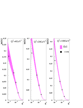
Figure 1: The strange distribution in fit1 at various $Q^{2}$ values.

In Fig. 1 we show the strange distribution at different $Q^{2}$ values. The results of the CCFR dimuon determination [4] is shown for comparison. The meaning of the error bands is explained in detail in Ref. 1. They correspond to an increase of the $\mathchar 28959\relax^{2}$ by one unit and do not take into account the uncertainties related to the choice of the functional form of the distributions. Note that although the CCFR points seem to be in good agreement with our curves, the strange-to-non-strange ratio we find is quite different from CCFR’s: $\mathchar 28948\relax=0.67$ at $Q^{2}=20$ GeV², to be compared with the CCFR value 0.48 at the same scale. We also performed a modified fit, called fit1b, imposing, as it is done by CTEQ and MRST, the condition $s+\bar{s}=0.5(\bar{u}+\bar{d})$, motivated by the CCFR result on $\mathchar 28948\relax$. It turns out that fit1b is definitely worse (see Tab. 1). We found that it is especially the $\bar{\mathchar 28951\relax}$ data which favor fit1 with respect to fit1b.

Table 1: The $\mathchar 28959\relax^{2}$’s of the three fits described in the text.

$\#$ pts	$\mathchar 28959\relax^{2}$ fit1	$\mathchar 28959\relax^{2}$ fit1b	$\mathchar 28959\relax^{2}$ fit2
2657	2430.8	2492.4	2405.0

Incidentally, we notice that no discrepancy whatsoever emerges in our fit between neutrino and charged-lepton data. We checked that the fit worsens if the CCFR structure functions data are taken into account.

5 Test of the charge asymmetry in the strange sea

Is $s(x)$ different in shape from $\bar{s}(x)$? In order to answer this question by fitting neutrino and antineutrino data one needs a good balance between $\mathchar 28951\relax$ and $\bar{\mathchar 28951\relax}$ statistics. This is the case of our data set.

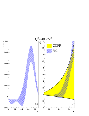
Figure 2: The strange vs. the antistrange distribution in fit2.

A charge asymmetry in the strange sea is not forbidden by first principles (clearly, as the nucleon has no net strangeness, one must have $\int{\rm d}x\,(s-\bar{s})=1$), and is actually expected in the framework of the intrinsic sea theory of Brodsky et al. [5]. Intrinsic $q\bar{q}$ pairs have a relatively long lifetime and arrange themselves into higher Fock states of the proton $|uudq\bar{q}\ldots\rangle$. By minimizing the kinetic energy on the light-cone one finds that the larger the mass of the intrinsic quark the higher its average momentum. Thus the intrinsic sea tends to occupy the large $x$ region. In the specific case of the strange sea, the $s\bar{s}$ pairs give rise to $N\to\Lambda K$ fluctuations [6]. In Ref. 7 it was shown, by simple chiral symmetry arguments, that one should expect $\langle x_{s}\rangle>\langle x_{\bar{s}}\rangle$.

In order to test the charge asymmetry of the strange sea, we released the constraint $s=\bar{s}$ and performed another fit, fit2, looking for a possible difference between $s(x)$ and $\bar{s}(x)$. In Fig. 2 we plot $xs(x)-x\bar{s}(x)$ and $s(x)/\bar{s}(x)$ at $Q^{2}=20$ GeV². The strange distribution turns out to be harder than the anti-strange one, in agreement with the expectation of the intrinsic sea theory. In Fig. 3 we show the difference $\Delta_{\mathchar 28951\relax}$ between $\mathchar 28951\relax$ and $\bar{\mathchar 28951\relax}$ differential cross sections which is directly sensitive to $s-\bar{s}$: fit2 is favored at large $x$ with respect to fit1. One can see in Table 1 that the minimum $\mathchar 28959\relax^{2}$ of fit2 is 25 units smaller than the $\mathchar 28959\relax^{2}$ of fit1, with an overall number of 2657 data points. It is clear that new high-statistics $\mathchar 28951\relax$ and $\bar{\mathchar 28951\relax}$ data would allow to increase the significance of the result and to draw a more definite conclusion.

Figure 3: Difference between the $\mathchar 28951\relax$ and $\bar{\mathchar 28951\relax}$ differential cross sections. The solid line corresponds to fit2, the dashed line to fit1.

6 Conclusion

We have shown how the full use of available $\mathchar 28951\relax,\bar{\mathchar 28951\relax}$ cross sections provides important information on the flavor structure of the nucleon, in particular on the strange distribution. A proper analysis of the forthcoming neutrino data (CHORUS and NuTeV) will certainly improve our knowledge of $s(x)$ and allow a more conclusive test of the charge asymmetry of the strange sea.

Note added. After we submitted this paper to the LC99 Workshop, we became aware of the talk delivered by A. Bodek (on behalf of CCFR-NuTeV) at the Moriond meeting (March 2000)[8]. The CCFR–NuTeV Collaboration is carrying out the analysis of new $\mathchar 28951\relax,\bar{\mathchar 28951\relax}$ DIS measurements at Fermilab. Their preliminary results show that:

• it is crucial not to introduce any theoretical bias in extracting neutrino structure functions from cross sections (as we stressed in Ref. 1 and in the present contribution);

• a NLO analysis based on a massive scheme is needed in order to get reliable results, especially in the charm-strange sector (as it was anticipated longtime ago[9, 10]), and therefore the slow rescaling procedure should be definitely discarded;

• a large discrepancy emerges between the newly determined $F_{2}$ and the old CCFR $F_{2}$: this is a further, a posteriori, justification for our choice of not using the old CCFR data on $F_{2}$ in our fits;

• the disagreement between $\mathchar 28950\relax$ and $\mathchar 28951\relax$ data is solved by a consistent treatment of the data (which confirms what we claimed in Ref. 1);

• measuring the difference $xF_{3}^{\mathchar 28951\relax}-xF_{3}^{\bar{\mathchar 28951\relax}}$ is a viable method to extract the strange sea distribution (the advantages of this method were pointed out, from a theoretical viewpoint, in Ref. 11).

The hopefully imminent release of the CCFR-NuTeV cross section data will allow to push the program of Ref. 1 forward in the direction of a better understanding of the flavor structure of the proton.

References

References

- [1] V. Barone, C. Pascaud and F. Zomer, Eur. Phys. J. C 12, 243 (2000).
- [2] H.L. Lai et al., CTEQ Collaboration, Eur. Phys. J. C 12, 375 (2000).
- [3] A.D. Martin, R.G. Roberts, W.J. Stirling and R.S. Thorne, Eur. Phys. J. C 4, 463 (1998).
- [4] A.O. Bazarko et al., CCFR Collaboration, Z. Phys. C 65, 189 (1995).
- [5] S.J. Brodsky, C. Peterson and N. Sakai, Phys. Rev. D 23, 2745 (1981).
-
[6]
A.I. Signal and A.W. Thomas, Phys. Lett. B 191, 205 (1987).
S.J. Brodsky and B.-Q. Ma, Phys. Lett. B 381, 317 (1996). - [7] M. Burkardt and B.J. Warr, Phys. Rev. D 45, 958 (1992).
-
[8]
See the transparencies of Bodek’s talk at
http://moriond.in2p3.fr/QCD00/transparencies/6friday/am/bodek - [9] M.G. Aivazis, F.I. Olness and W.-K. Tung, Phys. Rev. Lett. 65 (1990) 2339.
- [10] V. Barone et al., Phys. Lett. B 268 (1991) 279; Z. Phys. C 70 (1996) 83.
- [11] V. Barone, U. D’Alesio and M. Genovese, Phys. Lett. B 357 (1995) 435.