Towards a solution of the charmonium production controversy: $k_{\perp}$-factorization versus color octet mechanism

Abstract

The cross section of $\chi_{cJ}$ hadroproduction is calculated in the $k_{\perp}$ -factorization approach. We find a significant contribution of the $\chi_{c1}$ state due to non-applicability of the Landau-Yang theorem because of off-shell gluons. The results are in agreement with data and in contrast to the collinear factorization show a dominance of the color singlet part and a strong suppression of the color octet contribution. Our results could therefore lead to a solution of the longstanding controversy between the color singlet model and the color octet mechanism.

20.09.2000

The production of heavy quarkonia received a lot of attention from both theory and experiment in recent years. It is e.g. the most prominent signal in the search for the quark gluon plasma. Its usefullness is, however, questionable as long as the charmonium production process is not understood. For a review we refer to [1, 2, 3]. Originally heavy quarkonium production was described in the color singlet model (CSM) [4, 5]. Calculations based on this model and standard collinear factorization show however disagreement with the experimental data. For example the next-to-leading order (NLO) QCD collinear results for direct $J/\Psi$ hadroproduction underestimate the measured cross section at Tevatron by a factor of $\approx$ 50 (see fig.4 in [6] and Ref.[7]). The proposed solution to this strong discrepancy is the so called color-octet-mechanism (COM) [8, 9], according to which a color octet $q\overline{q}$-pair which has been produced at short distances can evolve into a physical quarkonium state by radiating soft gluons. The COM introduces uncalculable non-perturbative parameters, the color octet matrix elements, which have to be determined by a fit to the data [10, 11]. The inclusion of the COM into NLO QCD collinear calculations leads in the case of hadroproduction to a reasonable agreement with experiment [10, 11]. In these calculations the color octet contribution dominates.

On the other hand up to now the COM suffers at least from two unsolved problems. When the, supposedly universal, color octet matrix elements are applied to electroproduction of heavy quarkonium the theoretical predictions fail to describe the data [12]. Furthermore the results of the COM for polarized heavy quarkonium hadroproduction seem to be incompatible with recent data from Tevatron [13].

The longstanding discrepancy between the results based on the CSM together with collinear factorization and the experimental data shows up especially strongly in the $k_{\perp}$-dependent cross sections from Tevatron [6]. Thus one can wonder if the collinear approximation, in which in NLO the only transverse momentum of the produced quarkonium comes from an additional final state gluon, is suitable at all.

The aim of our paper is to clarify this question by a study of $\chi_{cJ}$ hadroproduction within the $k_{\perp}$ -factorization approach, which takes the nonvanishing transverse momenta of the colliding t-channel gluons into account. Generically this corresponds to taking into account new regions of the phase space of the colliding gluons which is mandatory for the description of hard processes in the Regge region.

More precisely we calculate the production of $J/\Psi$’s originating from radiative $\chi_{cJ}$ decays. In a recent study [14] of open $b\bar{b}$ hadroproduction we found that $k_{\perp}$ -factorization gives far better results than NLO collinear QCD calculations and we expect a similar improvement for heavy quarkonium production. The main ingredients of our calculations in [14] are the unintegrated gluon distribution and the effective next-to-leading-logarithmic-approximation (NLLA) $q\overline{q}$ -BFKL production vertex which we use in this article as well. The projection of the heavy quark-antiquark pair onto the corresponding charmonium state is described in the standard way within the non-relativistic-quarkonium-model [5, 4, 10, 11].

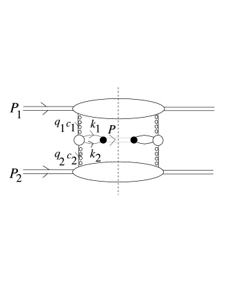
FIG. 1.: The basic diagram

We study the production of $\chi_{cJ}$ whose lowest Fock state component is $q\overline{q}(^{3}P_{J})$. For $J/\Psi$ (a $q\overline{q}(^{3}S_{1})$ state) the LO production amplitude is zero. In order to get a nonzero $q\overline{q}(^{3}S_{1})$-amplitude one has (in NLO in $\alpha_{S}$) to emit an additional gluon. The amplitude for the production of a $q\overline{q}$ -pair plus a gluon within the BFKL approach would in our case require an effective three-particle production vertex which still has to be derived. In contrast the production of a $\chi_{c1}$ can be calculated in our approach in LO because the Landau-Yang theorem which usually forbids the production of a ${}^{3}P_{1}$ state is not valid for off-mass-shell gluons.

We use the following definition of the light cone coordinates

$\displaystyle k^{+}=k^{0}+k^{3},\text{ }k^{-}=k^{0}-k^{3},\text{ }k_{\perp}=(0,k^{1},k^{2},0)=(0,{\bf k,}0{\bf)}.$

In the c.m. frame the momenta of the scattering hadrons are given by

$\displaystyle P_{1}^{+}=P_{2}^{-}=\sqrt{s},\text{ \ }P_{1}^{-}=P_{2}^{+}=P_{1\perp}=P_{2\perp}=0,$

where the Mandelstam variable $s$ is as usual the c.m.s. energy squared. The momenta of the t-channel gluons are $q_{1}$ and $q_{2}$ (see Fig.1). The on-shell quark and antiquark (with mass $m$) have momentum $k_{1}$ respectively $k_{2}$ with

$\displaystyle k_{1}^{-}=\frac{(m^{2}-k_{1\perp}^{2})}{k_{1}^{+}},\text{ \ }k_{2}^{-}=\frac{(m^{2}-k_{2\perp}^{2})}{k_{2}^{+}}.$

In the high energy (large $s$) regime we have

$$P^{+}\!=q_{1}^{+}-q_{2}^{+}\approx q_{1}^{+},\;P^{-}\!=q_{1}^{-}-q_{2}^{-}\approx-q_{2}^{-},\;q_{1/2}^{2}\approx q_{1/2\perp}^{2},$$

where $P=k_{1}+k_{2}$ is the momentum of the heavy quarkonium with $P^{2}=4m^{2}$. The longitudinal momentum fractions of the gluons are $x_{1}=q_{1}^{+}/P_{1}^{+}$, $x_{2}=-q_{2}^{-}/P_{2}^{-}$.

The heavy quarkonium hadroproduction cross section in the $k_{\perp}$-factorization approach is [17], [18]

$$\sigma_{P_{1}P_{2}\rightarrow\chi X}=\frac{1}{8(2\pi)}\!\!\int\!\!\frac{d^{3}P}{P^{+}}d^{2}q_{1\perp}d^{2}q_{2\perp}\delta^{2}(q_{1\perp}-q_{2\perp}-P_{\perp})$$ (1)

$${\cal F}(x_{1},q_{1\perp})\frac{1}{(q_{1\perp}^{2})^{2}}\left\{\frac{\psi_{\chi}^{\dagger c_{2}c_{1}}\psi_{\chi}^{c_{2}c_{1}}}{(N_{C}^{2}-1)^{2}}\right\}\frac{1}{(q_{2\perp}^{2})^{2}}{\cal F}(x_{2},q_{2\perp}).$$ (2)

The factor $(N_{C}^{2}-1)^{2}$ comes from the projection on color singlet in the t-channel. ${\cal F}(x,q_{\perp})$ is the unintegrated gluon distribution. The heavy quarkonium production amplitude $\psi_{\chi}^{c_{2}c_{1}}(x_{1},x_{2},q_{1\perp},q_{2\perp},P)$ is factorized (see below) in a hard part which describes the production of the $q\overline{q}$ pair and an amplitude describing the binding of this pair into a physical charmonium state. We choose the scale $\mu^{2}$ for $\alpha_{S}(\mu^{2})$ in the amplitude $\psi_{\chi}^{c_{2}c_{1}}$ to be ${\bf q}_{1}^{2}=-q_{1\perp}^{2}$ respectively ${\bf q}_{2}^{2}=-q_{2\perp}^{2}$ [19].

The amplitude for the production of the charmonium state can be written as

$$\psi_{\chi}^{c_{2}c_{1}}={\cal P}(q\overline{q}\rightarrow\chi_{cJ})\bullet\Psi^{c_{2}c_{1}}.$$ (3)

The $q\bar{q}$ production vertex $\Psi^{c_{2}c_{1}}$ derived in [20] for massless QCD, appropriately generalized for massive quarks, has the form

$\displaystyle\Psi^{c_{2}c_{1}}=-g^{2}\left(t^{c_{1}}t^{c_{2}}\,b(k_{1},k_{2})-t^{c_{2}}t^{c_{1}}\,b^{T}(k_{2},k_{1})\right),$

where $t^{c}$ are the colour group generators in the fundamental representation. The operator ${\cal P}(q\overline{q}\rightarrow\chi_{cJ})$ projects the $q\bar{q}$ pair onto the charmonium bound state, see below.

The functions $b(k_{1},k_{2})$ and $b^{T}(k_{2},k_{1})$ are illustrated in Fig.2 and their explicit form can be found in [14]. One important property of the charmonium production amplitude for on-mass-shell quark and antiquark states (3), which is related to the gauge invariance of the whole approach, is its vanishing in the limit $q_{1\perp}\rightarrow 0$ (or $q_{2\perp}\rightarrow 0$).

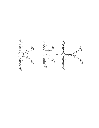
FIG. 2.: The effective vertex

The relation between the usual gluon distribution $xg(x,{\bf q}^{2})$ and the unintegrated gluon distribution ${\cal F}(x,{\bf k})$ is given by

$$xg(x,{\bf q}^{2})=\int_{0}^{\infty}\frac{d{\bf k}^{2}}{{\bf k}^{2}}\Theta({\bf q}^{2}-{\bf k}^{2}){\cal F}(x,{\bf k}).$$ (4)

${\cal F}(x,{\bf k})$ includes the evolution in $x$ and ${\bf k}^{2}$ described by the BFKL and DGLAP equation. In the non-perturbative region of small ${\bf k}^{2}$ the unintegrated gluon distribution is not known, therefore we write (4) according to [21, 18, 22, 23] as

$\displaystyle xg(x,{\bf q}^{2})=xg(x,{\bf q}_{0}^{2})+\int_{{\bf q}_{0}^{2}}^{\infty}\frac{d{\bf k}^{2}}{{\bf k}^{2}}\Theta({\bf q}^{2}-{\bf k}^{2}){\cal F}(x,{\bf k}),$

which introduces the a priori unknown initial scale ${\bf q}_{0}$ and the initial gluon distribution $xg(x,{\bf q}_{0}^{2})$. Following [21, 22], we neglect the momentum dependence of the hard cross section in the soft region $|{\bf q}|<|{\bf q}_{0}|$, so that

$$\frac{1}{q_{1\perp}^{2}}\left\{\frac{\psi_{\chi}^{\dagger c_{2}c_{1}}\psi_{\chi}^{c_{2}c_{1}}}{(N_{C}^{2}-1)^{2}}\right\}\frac{1}{q_{2\perp}^{2}}\equiv S(q_{1\perp},q_{2\perp})\to$$

$$\left[S(q_{1\perp},q_{2\perp})\Theta({\bf q}_{2}^{2}-{\bf q}_{0}^{2})+S(q_{1\perp},0)\Theta({\bf q}_{0}^{2}-{\bf q}_{2}^{2})\right]\Theta({\bf q}_{1}^{2}-{\bf q}_{0}^{2})$$

$$+\left[S(0,q_{2\perp})\Theta({\bf q}_{2}^{2}-{\bf q}_{0}^{2})+S(0,0)\Theta({\bf q}_{0}^{2}-{\bf q}_{2}^{2})\right]\Theta({\bf q}_{0}^{2}-{\bf q}_{1}^{2}),$$

see also the discussion of this expression in [14].

One important point is the proper choice of the unintegrated gluon distribution function. We use the results of Kwiecinski, Martin and Stas̀to [15]. They determined it using a combination of DGLAP and BFKL evolution equations. With the initial conditions

$${\bf q}_{0}^{2}=1\text{ GeV},\ xg(x,{\bf q}_{0}^{2})=1.57(1-x)^{2.5}.$$ (5)

they obtained an execellent fit to $F_{2}(x,Q^{2})$ data over a large range of $x$ and $Q^{2}$.

In order to see the effect of off-shell gluons and the inapplicability of the Landau-Yang theorem as well as to perform calculations which do not require a fit to the data we start with calculation of the color singlet part of the amplitude. This is most easily done by adapting the method of [4, 5]. The projection of the hard amplitude onto the charmonium bound state is given by

$$\psi_{\chi}^{c_{2}c_{1}}={\cal P}(q\overline{q}\rightarrow\chi_{cJ})\bullet\Psi^{c_{2}c_{1}}$$ (8)

$$=\sum_{i,j}\sum_{L_{z},S_{z}}\frac{1}{\sqrt{m}}\int\frac{d^{4}q}{(2\pi)^{4}}\delta\left(q^{0}-\frac{\vec{q}^{2}}{M}\right)\Phi_{L=1,L_{z}}(\vec{q})$$

$$\left\langle L=1,L_{z},S=1,S_{z}|J,J_{z}\right\rangle\left\langle 3i,\bar{3}j|1\right\rangle Tr\left\{\Psi_{ij}^{c_{2}c_{1}}{\cal P}_{S=1,S_{z}}\right\},$$

(9)

where $\Phi_{L=1,L_{z}}(\vec{q}=\vec{k}_{1}-\vec{k}_{2})$ is the momentum space wave function of the charmonium, and the projection operator ${\cal P}_{S=1,S_{z}}$ for a small relative momentum $q=k_{1}-k_{2}$ has the form

$\displaystyle{\cal P}_{S=1,S_{z}}=\frac{1}{2m}(\not{k}_{2}-m)\frac{\not{\epsilon}(S_{z})}{\sqrt{2}}(\not{k}_{1}+m).$

The Clebsch-Gordan coefficient in color space is given by $\left\langle 3i,\bar{3}j|1\right\rangle=\delta_{ji}/\sqrt{N_{C}}$. Since $P$-waves vanish at the origin, one has to expand the trace in (9) in a Taylor series around $\vec{q}=0$. This yields an expression proportional to

$\displaystyle\int\frac{d^{3}\vec{q}}{(2\pi)^{3}}q^{\alpha}\Phi_{L=1,L_{z}}(\vec{q})=-i\sqrt{\frac{3}{4\pi}}\epsilon^{\alpha}(L_{z}){\cal R}^{\prime}(0),$

with the derivative of the $P$-wave radial wave function at the origin ${\cal R}^{\prime}(0)$ whose numerical values can be found in [16]. For the individual $\chi_{cJ=1}$ and $\chi_{cJ=2}$ amplitudes we use

$$\sum_{L_{z},S_{z}}\!\!\left\langle 1,L_{z},1,S_{z}|1,J_{z}\right\rangle\epsilon^{\mu}(L_{z})\epsilon^{\nu}(S_{z})\!=\!-i\sqrt{\frac{1}{2}}\varepsilon^{\mu\nu\alpha\beta}\frac{P_{\alpha}}{M}\epsilon_{\beta}(J_{z})$$

$$\sum_{L_{z},S_{z}}\!\!\left\langle 1,L_{z},1,S_{z}|2,J_{z}\right\rangle\epsilon^{\mu}(L_{z})\epsilon^{\nu}(S_{z})=\epsilon^{\mu\nu}(J_{z})$$

where we introduce the spin 1 and spin 2 polarization tensors $\epsilon_{\beta}(J_{z})$ and $\epsilon^{\mu\nu}(J_{z})$ of the produced charmonium $\chi_{cJ=1}$ respectively $\chi_{cJ=2}$. In the unpolarized case the squared amplitudes are further evaluated using

$$\sum_{J_{z}}\epsilon^{\mu}(J_{z})\epsilon^{\nu}(J_{z}) = -g^{\mu\nu}+\frac{P^{\mu}P^{\nu}}{M^{2}}=P^{\mu\nu},$$

$$\sum_{J_{z}}\epsilon^{\mu\nu}(J_{z})\epsilon^{\alpha\beta}(J_{z}) = \frac{1}{2}\left(P^{\mu\alpha}P^{\nu\beta}+P^{\nu\alpha}P^{\mu\beta}\right)-\frac{1}{3}P^{\mu\nu}P^{\alpha\beta}.$$

The cross section for $J/\Psi$ production from radiative $\chi_{cJ}$ decays is then given by [10, 11]

$\displaystyle\sigma_{J/\Psi\ from\ \chi_{c}}=\sum_{J=0,1,2}\sigma_{P_{1}P_{2}\rightarrow\chi_{cJ}X}\cdot Br(\chi_{cJ}\rightarrow J/\Psi+\gamma),$

with the $\chi_{cJ}$ hadroproduction cross section $\sigma_{P_{1}P_{2}\rightarrow\chi_{cJ}X}$ (2). Because of the small branching ratio $Br(\chi_{cJ=0}\rightarrow J/\Psi+\gamma)={\cal O}(10^{-3})$ the contribution from $\chi_{cJ=0}$ is negligible. For the numerical computation we use the values

$$m_{c}=1.48\text{ GeV,}\;\;|{\cal R}^{\prime}(0)|^{2}=0.075\text{ GeV}^{5}.$$

The pseudorapidity is defined as $\eta=\frac{1}{2}\ln\left((\sqrt{P_{0}^{2}-M^{2}}+P_{3})/(\sqrt{P_{0}^{2}-M^{2}}-P_{3})\right)$. To compare with data we multiply our cross sections with the braching ratio $Br(J/\Psi\rightarrow\mu^{+}\mu^{-})$.

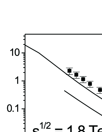
FIG. 3.: The transverse momentum differential cross section in comparison to the data and a NLO QCD calculation

The resulting $P_{\perp}$-dependent cross section for $J/\Psi$’s from radiative deacays of $\chi_{c}$’s produced in $pp$-collisions is shown in Fig.3 together with the data from the CDF Collaboration [6] and a NLO QCD collinear result (see Fig.7 in [11]). The individual contributions from $\chi_{c1}$ and $\chi_{c2}$ are shown in Fig.4.

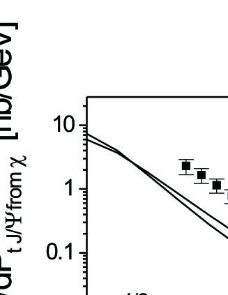
FIG. 4.: The individual contributions from $\chi_{c1}$ and $\chi_{c2}$

The description of the data by the color singlet part alone is very satisfactory and becomes even better if the difference of the transverse momentum of $J/\Psi$ (which is measured experimentally) and $\chi_{c}$ (which enters our calculation) is taken into account. (Due to the radiative decay the transverse momentum of $J/\Psi$ is typically larger by an amount of $\approx 300$ MeV than the corresponding $\chi_{c}$ one which leads to a shift of the theoretical curve to the right.) The typical scale of the gluon off-shellness is given by the transverse momentum of the produced quarkonium.

We emphasize that the result has been obtained without fitting any of the parameters involved: The unintegrated gluon distribution has been adopted from Kwiecinski et al. [15]. The parameters of the quarkonium bound state are the ones given by Eichten and Quigg [16]. For the $\chi_{c1}$ state it is crucial that the gluons are off-shell in $k_{\perp}$ -factorization.

FIG. 5.: The color octet contribution

Now we proceed with the calculation of $J/\Psi$ production by $\chi_{c}$ radiative decays adopting the colour octet mechanism. The infrared stability of higher order corrections to the cross section requires the existence of a color octet contribution, without fixing its size [9]. The $\chi_{c}$ state can be written in a velocity expansion as [10]

$\displaystyle\left|\chi_{c}\right\rangle={\cal O}(1)\left|q\overline{q}\left[{}^{3}P_{J}^{\text{ }1}\right]\right\rangle+{\cal O}({\bf v})\left|q\overline{q}\left[{}^{3}S_{1}^{8}\right]g\right\rangle+\cdot\cdot\cdot.$

Following the formalism of [10, 11] the resulting cross section is then proportional to the color octet matrix element $\left\langle 0\right|O_{8}^{\chi_{c1}}(^{3}S_{1})\left|0\right\rangle$ which has to be fitted to data. Using the results for the color singlet part and adding the color octet contribution we obtain as value of the color octet matrix element $\left\langle 0\right|O_{8}^{\chi_{c1}}(^{3}S_{1})\left|0\right\rangle=(9.0\pm 2.0)\times 10^{-4}.$ Comparing this with the result obtained in the collinear factorization [10, 11] we find a suppression of the matrix element due to the flat $P_{\perp}$-dependence of the color octet contribution by roughly one order of magnitude, resulting in a violation of the velocity scaling rules. These scaling rules are derived rigorously in the framework of non-relativistic QCD (NRQCD) [9]. It is, therefore, natural to assume that the charm quark is simply not heavy enough for the velocity scaling rules of NRQCD to be valid. This is also suggested by other observations, see e.g. the very recent study [24]. In contrast the description of bottom systems in NRQCD should be more accurate. This shows the importance of a detailed analysis of bottomonia production in the $k_{\perp}$-factorization approach.

Let us conclude. The $k_{\perp}$-factorization approach relying on an unintegrated gluon distribution compatible with the small $x$ behaviour of the structure function $F_{2}$ together with the BFKL NLLA fermion production vertices describes correctly $\chi_{c}$ production in the central rapidity region. Whereas the standard collinear factorization approach in NLO can describe the data in the TeV range only by introducing a dominant octet contribution, we have shown that in the $k_{\perp}$-factorization approach such a contribution gives an improved description of the data but is suppressed by its $P_{\perp}$ behaviour.

Our main conclusion is therefore that the correct way to improve the standard QCD calculations for quarkonium production in the TeV range is to abandon the collinear approximation. The contributions disregarded in the collinear approximation of strong transverse momentum ordering become essential in the small-$x$ range. The relative merits of the $k_{\perp}$ -factorization as the standard approach for other processes in high energy hadronic collisions still has to be investigated.

L.Sz. and O.V.T. thank A. Tkabladze for discussion.

The work is supported by the DFG.

REFERENCES

• [1] G.A. Schuler, CERN-TH-7170-94, hep-ph/9403387
• [2] E. Braaten, S. Flemming, T.C. Yuan, Ann.Rev.Nucl. Part.Sci.46 (1996) 197
• [3] Bottom Production, Proceedings of Workshop on Standard Model Physics at the LHC, Geneva, Switzerland 1999, hep-ph/0003142
• [4] R. Baier, R. RΓΌckl, Z.Phys. C19(1983) 251
• [5] B. Guberina, J.H. Kuhn, R.D. Peccei, R. RΓΌckl, Nucl.Phys. B174(1980) 317
• [6] Abe et al., CDF Collaboration, FERMILAB-Conf-95/226-E
• [7] Abe et al., Phys.Rev.Lett.79(1997) 578
• [8] E. Braaten, S. Fleming, Phys.Rev.Lett. 74 (1995) 3327
• [9] G.T. Bodwin, E. Braaten, G.P. Lepage, Phys.Rev. D51 (1995) 1125, Erratum-ibid. D55(1997) 5853
• [10] P. Cho, A.K. Leibovich, Phys.Rev. D53(1996) 150
• [11] P. Cho, A.K. Leibovich, Phys.Rev. D53(1996) 6203
• [12] T. Carli, Latest Highlights from H1 Collaboration, hep-ph/9906540
• [13] J.K. Mizukoshi, The Paradox of Charmonium Production, hep-ph/9911384
• [14] Ph. HΓ€gler, R. Kirschner, A. SchΓ€fer, L. Szymanowski, O.V. Teryaev, Phys.Rev. D62(2000) 71502
• [15] J. Kwiecinski, A.D. Martin, A.M. Stasto, Phys.Rev. D56(1997) 3991
• [16] E.J. Eichten, Ch. Quigg, Phys.Rev. D52(1995) 1726
• [17] S. Catani, M. Ciafaloni, F. Hautmann, Phys. Lett. B242(1990) 97; Nucl. Phys. B366(1991) 135
• [18] J.C. Collins, R.K. Ellis, Nucl. Phys. B360(1991) 3
• [19] E.M. Levin, M.G. Ryskin, Yu.M. Shabelski, A.G. Shuvaev, Yad.Fiz. 54 (1991) 1420
• [20] V.S. Fadin, L.N. Lipatov, Nucl. Phys. B477(1996) 767
• [21] J. Kwiecinski, Z.Phys. C29(1985) 561
• [22] M.G. Ryskin, Yu.M. Shabelski, Z.Phys. C61(1994) 517
• [23] M.G. Ryskin, Yu.M. Shabelski, A.G. Shuvaev, Z.Phys. C69 (1996) 269
• [24] S. Fleming, I.Z. Rothstein, A.K. Leibovich, hep-ph/0012062