NORDITA-2000/43 HE LAPTH-793/00 hep-ph/0004234 April 26, 2000
Quarkonium Production through Hard Comover Scattering. II [1]

Abstract

We extend to large transverse momentum $p_{\perp}$ an approach to quarkonium hadroproduction previously suggested for low $p_{\perp}$. The dynamics involves a perturbative rescattering of the heavy quark pair off a comoving color field which originates from gluon radiation prior to the heavy quark production vertex. Assuming simple properties of the comoving field we find the rescattering scenario to be in reasonable agreement with data. At large $p_{\perp}$, $\psi^{\prime}$ is predicted to be unpolarized, and $\chi_{1}$ production is favoured compared to $\chi_{2}$. We predict the $\chi_{1}$ polarization to be transverse at low $p_{\perp}$, and to get a longitudinal component at large $p_{\perp}$.

]

I Introduction

Quarkonium production is a rich domain of QCD which involves several hardness scales, namely the transverse momentum $p_{\perp}$ of the heavy quark pair, the quark mass $m$ and the Bohr momentum of the heavy quarks in quarkonium $\alpha_{s}m$. Furthermore, bremsstrahlung gluons are produced along with the pair at an intermediate hardness scale. The proximity of the open flavour threshold makes the production of a quarkonium state highly sensitive to its production environment. Relatively soft rescatterings of the quark pair with surrounding fields can make or break the bound state.

Quarkonium production may be contrasted with open heavy flavour production, for which the total cross section is unaffected by late rescattering. This insensitivity is technically expressed through the QCD factorization theorem [2], which allows the cross section to be written in terms of process-independent parton distributions. An analogous factorization of hard and soft physics does not apply to quarkonium production rates, which constitute a small fraction of the total open flavour cross section. This makes quarkonium physics a challenging and potentially rewarding field which can teach us new aspects of the dynamics of hard processes.

Attempts to ignore rescattering effects in quarkonium production have met with success in photoproduction but failed in hadroproduction. The PQCD prediction for quarkonium production without rescattering, at lowest order in the quark pair relative velocity $v$ (the ‘Color Singlet Model’, CSM [3, 4]), accounts well for the HERA data on $\gamma p\to J/\psi X$ in the photon fragmentation region [5]. On the contrary, the CSM underestimates the Tevatron $\bar{p}p$ data on direct $J/\psi$ and $\psi^{\prime}$ production at large $p_{\perp}$ by a factor $\sim 50$ [6]. Similar discrepancies are also observed in hadroproduction at low $p_{\perp}$ [7].

The CSM amplitudes contain infrared divergencies, which for $P$-wave states appear already at lowest order in $\alpha_{s}$. The divergencies cancel systematically between terms of different orders in $v$, as shown by the ‘NRQCD’ [8] expansion of the amplitude. In the absence of rescattering effects NRQCD is thus a theoretically viable framework for calculating quarkonium production in QCD.

The NRQCD terms of higher order in $v$ correspond to relativistic effects in the quarkonium wave function, and are related to its higher Fock components such as $|{Q\bar{Q}g}\rangle$. The magnitude of the relativistic corrections is poorly known, and higher powers of $v$ may be compensated by lower powers of $\alpha_{s}$ at the hard vertex. Hence one may consider the possibility that the observed discrepancies between the CSM and hadroproduction data are due to higher order contributions in the NRQCD expansion (the ‘Color Octet Model’, COM [9]). This implies, however, new contributions also in photoproduction which tends to lead to an overestimate of the data [5]. The phenomenological difficulties of a COM approach [10, 11] have recently been made more acute by the (preliminary) CDF data on $\psi^{\prime}$ polarization at large $p_{\perp}$ [12]. The COM prediction of a transverse $\psi^{\prime}$ polarization, considered as a crucial test of the COM approach, fails by more than 3 standard deviations [13].

It would thus appear that rescattering is important in quarkonium hadroproduction. Since gluons, unlike photons, carry a comoving color field one expects more rescattering in hadroproduction than in photoproduction. In [10] (referred to as I in the following) a scenario involving a perturbative rescattering of $Q\bar{Q}$ pairs produced at low $p_{\perp}\lesssim m$ was studied. A simple form of the comoving field allowed several of the puzzling features of the data to be understood.

Here we shall extend the rescattering picture of I to quarkonium production at high $p_{\perp}$. We refer to I for a detailed discussion of the rescattering mechanism and its phenomenological justification. In section II we present the low $p_{\perp}$ calculation in a more compact form than in I and recall the results which were obtained. In section III we propose a generalization of the low $p_{\perp}$ approach to high $p_{\perp}$, and evaluate $S$-wave and $P$-wave quarkonium production amplitudes. All results obtained within the rescattering picture (at low and high $p_{\perp}$) are summarized in section IV, together with a discussion of our assumptions.

II Low $p_{\perp}$ Quarkonium Production

A Physical picture

The rescattering mechanism of quarkonium hadroproduction proposed in I is based on an interaction of the heavy quark pair with a comoving color field. Let us recall why a color field comoving with the $Q\bar{Q}$ pair may be created in hadroproduction, but not in photoproduction.

In the QED process $e^{+}e^{-}\to\mu^{+}\mu^{-}$ near threshold (Fig. 1a), the incoming electrons are surrounded by an electromagnetic (photon) field. As the electrons annihilate, these fields pass through each other without interacting (except via ${\cal O}(\alpha_{em})$ processes). The $\mu^{+}\mu^{-}$ pair is thus created in a field-free environment.

In the analogous QCD process $gg\to Q\bar{Q}$ (Fig. 1b), the color fields associated with the color charge of the colliding gluons on the contrary interact strongly. Such multiple interactions may create a remnant color field with low rapidity components in the $Q\bar{Q}$ rest frame. Rescattering may occur between this remnant field and the $Q\bar{Q}$ pair.

In photoproduction, $\gamma g\to Q\bar{Q}$ (Fig. 1c), the (unresolved) photon carries no radiation field and the situation is analogous to QED: no remnant field is comoving with the $Q\bar{Q}$ pair. Rescattering thus occurs only in hadroproduction, and may explain some of the observed ‘anomalies’ of quarkonium production. It is absent in photoproduction (except for resolved photon contributions), where the CSM predictions in fact are quite satisfactory.

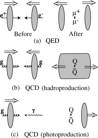
FIG. 1.: Scenario for the creation of a comoving color field in low $p_{\perp}$ hadroproduction.

B The model

The effects on low $p_{\perp}$ quarkonium hadroproduction of a rescattering of the $Q\bar{Q}$ pair off a comoving color field were studied in I in the framework of a simple model. Before extending this scenario to quarkonium production at high $p_{\perp}$ we summarize the main results of I.

The model applies to high energy production, where the quarkonium carries a moderate fraction $x_{F}$ of the hadron beam momentum and has $p_{\perp}\sim m$, where $m$ is the heavy quark mass. The amplitude for quarkonium production in the bound state rest frame shown in Fig. 2,

$${\cal M} = \sum_{L_{z},S_{z}}\langle LL_{z};SS_{z}|JJ_{z}\rangle\sum_{{\lambda\bar{\lambda}},{\sigma\bar{\sigma}}}\int\frac{d^{3}\mathchoice{{\hbox{\boldmath$\displaystyle p$}}}{{\hbox{\boldmath$\textstyle p$}}}{{\hbox{\boldmath$\scriptstyle p$}}}{{\hbox{\boldmath$\scriptscriptstyle p$}}}}{(2\pi)^{3}}\frac{d^{3}\mathchoice{{\hbox{\boldmath$\displaystyle p$}}}{{\hbox{\boldmath$\textstyle p$}}}{{\hbox{\boldmath$\scriptstyle p$}}}{{\hbox{\boldmath$\scriptscriptstyle p$}}}^{\prime}}{(2\pi)^{3}}d^{3}\mathchoice{{\hbox{\boldmath$\displaystyle q$}}}{{\hbox{\boldmath$\textstyle q$}}}{{\hbox{\boldmath$\scriptstyle q$}}}{{\hbox{\boldmath$\scriptscriptstyle q$}}}$$ (1)

$$\times \delta^{3}(\mathchoice{{\hbox{\boldmath$\displaystyle p$}}}{{\hbox{\boldmath$\textstyle p$}}}{{\hbox{\boldmath$\scriptstyle p$}}}{{\hbox{\boldmath$\scriptscriptstyle p$}}}+\mathchoice{{\hbox{\boldmath$\displaystyle p$}}}{{\hbox{\boldmath$\textstyle p$}}}{{\hbox{\boldmath$\scriptstyle p$}}}{{\hbox{\boldmath$\scriptscriptstyle p$}}}^{\prime}+\mathchoice{{\hbox{\boldmath$\displaystyle\ell$}}}{{\hbox{\boldmath$\textstyle\ell$}}}{{\hbox{\boldmath$\scriptstyle\ell$}}}{{\hbox{\boldmath$\scriptscriptstyle\ell$}}})\Phi_{\lambda\bar{\lambda}}^{[8]}(\mathchoice{{\hbox{\boldmath$\displaystyle p$}}}{{\hbox{\boldmath$\textstyle p$}}}{{\hbox{\boldmath$\scriptstyle p$}}}{{\hbox{\boldmath$\scriptscriptstyle p$}}},\mathchoice{{\hbox{\boldmath$\displaystyle p$}}}{{\hbox{\boldmath$\textstyle p$}}}{{\hbox{\boldmath$\scriptstyle p$}}}{{\hbox{\boldmath$\scriptscriptstyle p$}}}^{\prime})\ {\cal R}_{{\lambda\bar{\lambda}},{\sigma\bar{\sigma}}}(\mathchoice{{\hbox{\boldmath$\displaystyle\ell$}}}{{\hbox{\boldmath$\textstyle\ell$}}}{{\hbox{\boldmath$\scriptstyle\ell$}}}{{\hbox{\boldmath$\scriptscriptstyle\ell$}}},\mathchoice{{\hbox{\boldmath$\displaystyle p$}}}{{\hbox{\boldmath$\textstyle p$}}}{{\hbox{\boldmath$\scriptstyle p$}}}{{\hbox{\boldmath$\scriptscriptstyle p$}}},\mathchoice{{\hbox{\boldmath$\displaystyle q$}}}{{\hbox{\boldmath$\textstyle q$}}}{{\hbox{\boldmath$\scriptstyle q$}}}{{\hbox{\boldmath$\scriptscriptstyle q$}}})\ {\Psi_{\sigma\bar{\sigma}}^{L_{z}S_{z}}(\mathchoice{{\hbox{\boldmath$\displaystyle q$}}}{{\hbox{\boldmath$\textstyle q$}}}{{\hbox{\boldmath$\scriptstyle q$}}}{{\hbox{\boldmath$\scriptscriptstyle q$}}})}^{*}$$ (2)

is a convolution of the $gg\to Q\bar{Q}$ color octet wave function $\Phi^{[8]}$, the kernel ${\cal R}$ describing the rescattering between the pair and the comoving color field, and the quarkonium wave function $\Psi$.

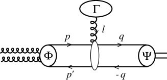
FIG. 2.: The low $p_{\perp}$ quarkonium production amplitude induced by a rescattering on the comoving field $\Gamma$ (two diagrams). From Ref.[10].

The $gg\to Q\bar{Q}$ process occurs on a proper time scale of order $m^{-1}$, whereas the time scale for quarkonium bound state formation is of order $(\alpha_{s}m)^{-1}$. The rescattering is assumed to be characterized by the ‘semi-hard’ scale $\mu$ of DGLAP gluon radiation

$$\alpha_{s}m\ll\mu\ll m$$ (4)

As a consequence, the rescattering is well separated in time from both the $Q\bar{Q}$ pair creation and the bound state formation. The heavy quarks thus propagate nearly on-shell both before and after the rescattering. In Eq. (LABEL:prodampl) the helicities and momenta of the quarks (in the quarkonium rest frame) before the rescattering are denoted $\lambda,\bar{\lambda}$ and $\mathchoice{{\hbox{\boldmath$\displaystyle p$}}}{{\hbox{\boldmath$\textstyle p$}}}{{\hbox{\boldmath$\scriptstyle p$}}}{{\hbox{\boldmath$\scriptscriptstyle p$}}},\mathchoice{{\hbox{\boldmath$\displaystyle p$}}}{{\hbox{\boldmath$\textstyle p$}}}{{\hbox{\boldmath$\scriptstyle p$}}}{{\hbox{\boldmath$\scriptscriptstyle p$}}}^{\prime}$. After the rescattering of momentum transfer $\textstyle\ell$ the same quantities are denoted by $\sigma,\bar{\sigma}$ and $\mathchoice{{\hbox{\boldmath$\displaystyle q$}}}{{\hbox{\boldmath$\textstyle q$}}}{{\hbox{\boldmath$\scriptstyle q$}}}{{\hbox{\boldmath$\scriptscriptstyle q$}}},-\mathchoice{{\hbox{\boldmath$\displaystyle q$}}}{{\hbox{\boldmath$\textstyle q$}}}{{\hbox{\boldmath$\scriptstyle q$}}}{{\hbox{\boldmath$\scriptscriptstyle q$}}}$. The calculation of I can be summarized by expressing every factor of (LABEL:prodampl) as a contraction between the spinors $\chi_{\lambda}$ and $\chi_{\lambda}^{\dagger}$, with $\chi_{+}^{\dagger}=\left(1\ 0\right)$, $\chi_{-}^{\dagger}=\left(0\ 1\right)$,

$$\Phi_{\lambda\bar{\lambda}}^{[8]}(\mathchoice{{\hbox{\boldmath$\displaystyle p$}}}{{\hbox{\boldmath$\textstyle p$}}}{{\hbox{\boldmath$\scriptstyle p$}}}{{\hbox{\boldmath$\scriptscriptstyle p$}}},\mathchoice{{\hbox{\boldmath$\displaystyle p$}}}{{\hbox{\boldmath$\textstyle p$}}}{{\hbox{\boldmath$\scriptstyle p$}}}{{\hbox{\boldmath$\scriptscriptstyle p$}}}^{\prime}) = \chi_{\lambda}^{\dagger}\,\tilde{\Phi}^{[8]}(\mathchoice{{\hbox{\boldmath$\displaystyle p$}}}{{\hbox{\boldmath$\textstyle p$}}}{{\hbox{\boldmath$\scriptstyle p$}}}{{\hbox{\boldmath$\scriptscriptstyle p$}}},\mathchoice{{\hbox{\boldmath$\displaystyle p$}}}{{\hbox{\boldmath$\textstyle p$}}}{{\hbox{\boldmath$\scriptstyle p$}}}{{\hbox{\boldmath$\scriptscriptstyle p$}}}^{\prime})\,\chi_{-\bar{\lambda}}$$ (6)

$${\cal R}_{{\lambda\bar{\lambda}},{\sigma\bar{\sigma}}}(\mathchoice{{\hbox{\boldmath$\displaystyle\ell$}}}{{\hbox{\boldmath$\textstyle\ell$}}}{{\hbox{\boldmath$\scriptstyle\ell$}}}{{\hbox{\boldmath$\scriptscriptstyle\ell$}}},\mathchoice{{\hbox{\boldmath$\displaystyle p$}}}{{\hbox{\boldmath$\textstyle p$}}}{{\hbox{\boldmath$\scriptstyle p$}}}{{\hbox{\boldmath$\scriptscriptstyle p$}}},\mathchoice{{\hbox{\boldmath$\displaystyle q$}}}{{\hbox{\boldmath$\textstyle q$}}}{{\hbox{\boldmath$\scriptstyle q$}}}{{\hbox{\boldmath$\scriptscriptstyle q$}}}) = (2\pi)^{3}\delta^{3}(\mathchoice{{\hbox{\boldmath$\displaystyle p$}}}{{\hbox{\boldmath$\textstyle p$}}}{{\hbox{\boldmath$\scriptstyle p$}}}{{\hbox{\boldmath$\scriptscriptstyle p$}}}-\mathchoice{{\hbox{\boldmath$\displaystyle q$}}}{{\hbox{\boldmath$\textstyle q$}}}{{\hbox{\boldmath$\scriptstyle q$}}}{{\hbox{\boldmath$\scriptscriptstyle q$}}}+\mathchoice{{\hbox{\boldmath$\displaystyle\ell$}}}{{\hbox{\boldmath$\textstyle\ell$}}}{{\hbox{\boldmath$\scriptstyle\ell$}}}{{\hbox{\boldmath$\scriptscriptstyle\ell$}}})\,\delta_{\bar{\lambda}}^{\bar{\sigma}}\,\chi_{\sigma}^{\dagger}\,\tilde{\cal R}^{Q}(\mathchoice{{\hbox{\boldmath$\displaystyle\ell$}}}{{\hbox{\boldmath$\textstyle\ell$}}}{{\hbox{\boldmath$\scriptstyle\ell$}}}{{\hbox{\boldmath$\scriptscriptstyle\ell$}}},\mathchoice{{\hbox{\boldmath$\displaystyle q$}}}{{\hbox{\boldmath$\textstyle q$}}}{{\hbox{\boldmath$\scriptstyle q$}}}{{\hbox{\boldmath$\scriptscriptstyle q$}}})\,\chi_{\lambda}$$ (7)

$$+ (2\pi)^{3} \delta^{3}(\mathchoice{{\hbox{\boldmath$\displaystyle p$}}}{{\hbox{\boldmath$\textstyle p$}}}{{\hbox{\boldmath$\scriptstyle p$}}}{{\hbox{\boldmath$\scriptscriptstyle p$}}}-\mathchoice{{\hbox{\boldmath$\displaystyle q$}}}{{\hbox{\boldmath$\textstyle q$}}}{{\hbox{\boldmath$\scriptstyle q$}}}{{\hbox{\boldmath$\scriptscriptstyle q$}}})\,\delta_{\lambda}^{\sigma}\,\chi_{-\bar{\lambda}}^{\dagger}\,\tilde{\cal R}^{\bar{Q}}(\mathchoice{{\hbox{\boldmath$\displaystyle\ell$}}}{{\hbox{\boldmath$\textstyle\ell$}}}{{\hbox{\boldmath$\scriptstyle\ell$}}}{{\hbox{\boldmath$\scriptscriptstyle\ell$}}},-\mathchoice{{\hbox{\boldmath$\displaystyle q$}}}{{\hbox{\boldmath$\textstyle q$}}}{{\hbox{\boldmath$\scriptstyle q$}}}{{\hbox{\boldmath$\scriptscriptstyle q$}}})\,\chi_{-\bar{\sigma}}$$ (8)

$${\Psi_{\sigma\bar{\sigma}}^{L_{z}S_{z}}(\mathchoice{{\hbox{\boldmath$\displaystyle q$}}}{{\hbox{\boldmath$\textstyle q$}}}{{\hbox{\boldmath$\scriptstyle q$}}}{{\hbox{\boldmath$\scriptscriptstyle q$}}})}^{*} = \frac{\Psi_{LL_{z}}^{*}(\mathchoice{{\hbox{\boldmath$\displaystyle q$}}}{{\hbox{\boldmath$\textstyle q$}}}{{\hbox{\boldmath$\scriptstyle q$}}}{{\hbox{\boldmath$\scriptscriptstyle q$}}})}{\sqrt{2}}\,\chi_{-\bar{\sigma}}^{\dagger}\,{\hat{e}}(S_{z})^{*}\,\chi_{\sigma}$$ (9)

In $\tilde{\cal R}^{Q}(\mathchoice{{\hbox{\boldmath$\displaystyle\ell$}}}{{\hbox{\boldmath$\textstyle\ell$}}}{{\hbox{\boldmath$\scriptstyle\ell$}}}{{\hbox{\boldmath$\scriptscriptstyle\ell$}}},\mathchoice{{\hbox{\boldmath$\displaystyle q$}}}{{\hbox{\boldmath$\textstyle q$}}}{{\hbox{\boldmath$\scriptstyle q$}}}{{\hbox{\boldmath$\scriptscriptstyle q$}}})$ and $\tilde{\cal R}^{\bar{Q}}(\mathchoice{{\hbox{\boldmath$\displaystyle\ell$}}}{{\hbox{\boldmath$\textstyle\ell$}}}{{\hbox{\boldmath$\scriptstyle\ell$}}}{{\hbox{\boldmath$\scriptscriptstyle\ell$}}},\mathchoice{{\hbox{\boldmath$\displaystyle q$}}}{{\hbox{\boldmath$\textstyle q$}}}{{\hbox{\boldmath$\scriptstyle q$}}}{{\hbox{\boldmath$\scriptscriptstyle q$}}})$, $\textstyle q$ stands for the momentum of the scattered quark or antiquark after the scattering. Eq. (9) holds for $S=1$ quarkonia, $\mathchoice{{\hbox{\boldmath$\displaystyle e$}}}{{\hbox{\boldmath$\textstyle e$}}}{{\hbox{\boldmath$\scriptstyle e$}}}{{\hbox{\boldmath$\scriptscriptstyle e$}}}(S_{z})$ being the bound state spin polarization vector defined in the rest frame as

$$\mathchoice{{\hbox{\boldmath$\displaystyle e$}}}{{\hbox{\boldmath$\textstyle e$}}}{{\hbox{\boldmath$\scriptstyle e$}}}{{\hbox{\boldmath$\scriptscriptstyle e$}}}(\pm 1) = (\mp 1,-i,0)/\sqrt{2}$$ (11)

$$\mathchoice{{\hbox{\boldmath$\displaystyle e$}}}{{\hbox{\boldmath$\textstyle e$}}}{{\hbox{\boldmath$\scriptstyle e$}}}{{\hbox{\boldmath$\scriptscriptstyle e$}}}(0) = (0,0,1)$$ (12)

We use the notation ${\hat{a}}=\mathchoice{{\hbox{\boldmath$\displaystyle a$}}}{{\hbox{\boldmath$\textstyle a$}}}{{\hbox{\boldmath$\scriptstyle a$}}}{{\hbox{\boldmath$\scriptscriptstyle a$}}}\cdot\mathchoice{{\hbox{\boldmath$\displaystyle\sigma$}}}{{\hbox{\boldmath$\textstyle\sigma$}}}{{\hbox{\boldmath$\scriptstyle\sigma$}}}{{\hbox{\boldmath$\scriptscriptstyle\sigma$}}}$ for a vector $\textstyle a$, with $\sigma_{k}$ the Pauli matrices. The amplitude (LABEL:prodampl) takes a form which can be readily inferred from Fig. 2,

$${\cal M}(S=1) = \sum_{L_{z},S_{z}}\langle LL_{z};SS_{z}|JJ_{z}\rangle\int\frac{d^{3}\mathchoice{{\hbox{\boldmath$\displaystyle q$}}}{{\hbox{\boldmath$\textstyle q$}}}{{\hbox{\boldmath$\scriptstyle q$}}}{{\hbox{\boldmath$\scriptscriptstyle q$}}}}{(2\pi)^{3}}\frac{\Psi_{LL_{z}}^{*}(\mathchoice{{\hbox{\boldmath$\displaystyle q$}}}{{\hbox{\boldmath$\textstyle q$}}}{{\hbox{\boldmath$\scriptstyle q$}}}{{\hbox{\boldmath$\scriptscriptstyle q$}}})}{\sqrt{2}}$$ (13)

$$\frac{1}{\sqrt{3}}T^{b}_{ji} \left\{{\rm Tr}\left[{\hat{e}}(S_{z})^{*}\tilde{\cal R}^{Q}(\mathchoice{{\hbox{\boldmath$\displaystyle\ell$}}}{{\hbox{\boldmath$\textstyle\ell$}}}{{\hbox{\boldmath$\scriptstyle\ell$}}}{{\hbox{\boldmath$\scriptscriptstyle\ell$}}},\mathchoice{{\hbox{\boldmath$\displaystyle q$}}}{{\hbox{\boldmath$\textstyle q$}}}{{\hbox{\boldmath$\scriptstyle q$}}}{{\hbox{\boldmath$\scriptscriptstyle q$}}})\tilde{\Phi}^{[8]}(\mathchoice{{\hbox{\boldmath$\displaystyle q$}}}{{\hbox{\boldmath$\textstyle q$}}}{{\hbox{\boldmath$\scriptstyle q$}}}{{\hbox{\boldmath$\scriptscriptstyle q$}}}-\mathchoice{{\hbox{\boldmath$\displaystyle\ell$}}}{{\hbox{\boldmath$\textstyle\ell$}}}{{\hbox{\boldmath$\scriptstyle\ell$}}}{{\hbox{\boldmath$\scriptscriptstyle\ell$}}},-\mathchoice{{\hbox{\boldmath$\displaystyle q$}}}{{\hbox{\boldmath$\textstyle q$}}}{{\hbox{\boldmath$\scriptstyle q$}}}{{\hbox{\boldmath$\scriptscriptstyle q$}}})\right]\right.$$ (14)

$$+ \left.{\rm Tr}\left[\tilde{\cal R}^{\bar{Q}}(\mathchoice{{\hbox{\boldmath$\displaystyle\ell$}}}{{\hbox{\boldmath$\textstyle\ell$}}}{{\hbox{\boldmath$\scriptstyle\ell$}}}{{\hbox{\boldmath$\scriptscriptstyle\ell$}}},-\mathchoice{{\hbox{\boldmath$\displaystyle q$}}}{{\hbox{\boldmath$\textstyle q$}}}{{\hbox{\boldmath$\scriptstyle q$}}}{{\hbox{\boldmath$\scriptscriptstyle q$}}}){\hat{e}}(S_{z})^{*}\tilde{\Phi}^{[8]}(\mathchoice{{\hbox{\boldmath$\displaystyle q$}}}{{\hbox{\boldmath$\textstyle q$}}}{{\hbox{\boldmath$\scriptstyle q$}}}{{\hbox{\boldmath$\scriptscriptstyle q$}}},-\mathchoice{{\hbox{\boldmath$\displaystyle q$}}}{{\hbox{\boldmath$\textstyle q$}}}{{\hbox{\boldmath$\scriptstyle q$}}}{{\hbox{\boldmath$\scriptscriptstyle q$}}}-\mathchoice{{\hbox{\boldmath$\displaystyle\ell$}}}{{\hbox{\boldmath$\textstyle\ell$}}}{{\hbox{\boldmath$\scriptstyle\ell$}}}{{\hbox{\boldmath$\scriptscriptstyle\ell$}}})\right]\right\}$$ (15)

where ${\rm Tr}$ denotes the trace of $2\times 2$ matrices. For convenience we separate the rescattering color factor from the kernel ${\cal R}$. The color indices of the rescattering gluon and of the quark and antiquark before the rescattering are denoted by $b$, $i$, $j$. The general form (13) will also be used in the case of high $p_{\perp}$ quarkonium production via gluon fragmentation in the next section.

In Eq. (13) the zeroth and first order terms in $\textstyle q$ correspond to $S$ and $P$-wave production, respectively. Recalling that $|\mathchoice{{\hbox{\boldmath$\displaystyle\ell$}}}{{\hbox{\boldmath$\textstyle\ell$}}}{{\hbox{\boldmath$\scriptstyle\ell$}}}{{\hbox{\boldmath$\scriptscriptstyle\ell$}}}|\sim\mu\ll m$ we work only to first order in the small quantities $\mathchoice{{\hbox{\boldmath$\displaystyle\ell$}}}{{\hbox{\boldmath$\textstyle\ell$}}}{{\hbox{\boldmath$\scriptstyle\ell$}}}{{\hbox{\boldmath$\scriptscriptstyle\ell$}}}/m$, $\mathchoice{{\hbox{\boldmath$\displaystyle q$}}}{{\hbox{\boldmath$\textstyle q$}}}{{\hbox{\boldmath$\scriptstyle q$}}}{{\hbox{\boldmath$\scriptscriptstyle q$}}}/m$. The rescattering kernel then reads [10]

$$\tilde{\cal R}^{Q,\bar{Q}}(\mathchoice{{\hbox{\boldmath$\displaystyle\ell$}}}{{\hbox{\boldmath$\textstyle\ell$}}}{{\hbox{\boldmath$\scriptstyle\ell$}}}{{\hbox{\boldmath$\scriptscriptstyle\ell$}}},\mathchoice{{\hbox{\boldmath$\displaystyle q$}}}{{\hbox{\boldmath$\textstyle q$}}}{{\hbox{\boldmath$\scriptstyle q$}}}{{\hbox{\boldmath$\scriptscriptstyle q$}}}) = \frac{g}{2m}\left[\mp iK+{\hat{G}}\right]$$ (17)

$$K(\mathchoice{{\hbox{\boldmath$\displaystyle\ell$}}}{{\hbox{\boldmath$\textstyle\ell$}}}{{\hbox{\boldmath$\scriptstyle\ell$}}}{{\hbox{\boldmath$\scriptscriptstyle\ell$}}},\mathchoice{{\hbox{\boldmath$\displaystyle q$}}}{{\hbox{\boldmath$\textstyle q$}}}{{\hbox{\boldmath$\scriptstyle q$}}}{{\hbox{\boldmath$\scriptscriptstyle q$}}}) = 2m\Gamma^{0}(\ell^{0},\mathchoice{{\hbox{\boldmath$\displaystyle\ell$}}}{{\hbox{\boldmath$\textstyle\ell$}}}{{\hbox{\boldmath$\scriptstyle\ell$}}}{{\hbox{\boldmath$\scriptscriptstyle\ell$}}})+\mathchoice{{\hbox{\boldmath$\displaystyle\Gamma$}}}{{\hbox{\boldmath$\textstyle\Gamma$}}}{{\hbox{\boldmath$\scriptstyle\Gamma$}}}{{\hbox{\boldmath$\scriptscriptstyle\Gamma$}}}(\ell^{0},\mathchoice{{\hbox{\boldmath$\displaystyle\ell$}}}{{\hbox{\boldmath$\textstyle\ell$}}}{{\hbox{\boldmath$\scriptstyle\ell$}}}{{\hbox{\boldmath$\scriptscriptstyle\ell$}}})\cdot(\mathchoice{{\hbox{\boldmath$\displaystyle\ell$}}}{{\hbox{\boldmath$\textstyle\ell$}}}{{\hbox{\boldmath$\scriptstyle\ell$}}}{{\hbox{\boldmath$\scriptscriptstyle\ell$}}}-2\mathchoice{{\hbox{\boldmath$\displaystyle q$}}}{{\hbox{\boldmath$\textstyle q$}}}{{\hbox{\boldmath$\scriptstyle q$}}}{{\hbox{\boldmath$\scriptscriptstyle q$}}})$$ (18)

$$\mathchoice{{\hbox{\boldmath$\displaystyle G$}}}{{\hbox{\boldmath$\textstyle G$}}}{{\hbox{\boldmath$\scriptstyle G$}}}{{\hbox{\boldmath$\scriptscriptstyle G$}}}(\mathchoice{{\hbox{\boldmath$\displaystyle\ell$}}}{{\hbox{\boldmath$\textstyle\ell$}}}{{\hbox{\boldmath$\scriptstyle\ell$}}}{{\hbox{\boldmath$\scriptscriptstyle\ell$}}}) = \mathchoice{{\hbox{\boldmath$\displaystyle\Gamma$}}}{{\hbox{\boldmath$\textstyle\Gamma$}}}{{\hbox{\boldmath$\scriptstyle\Gamma$}}}{{\hbox{\boldmath$\scriptscriptstyle\Gamma$}}}(\ell^{0},\mathchoice{{\hbox{\boldmath$\displaystyle\ell$}}}{{\hbox{\boldmath$\textstyle\ell$}}}{{\hbox{\boldmath$\scriptstyle\ell$}}}{{\hbox{\boldmath$\scriptscriptstyle\ell$}}})\times\mathchoice{{\hbox{\boldmath$\displaystyle\ell$}}}{{\hbox{\boldmath$\textstyle\ell$}}}{{\hbox{\boldmath$\scriptstyle\ell$}}}{{\hbox{\boldmath$\scriptscriptstyle\ell$}}}$$ (19)

The color field comoving with the $Q\bar{Q}$ pair is modelled as an external source $\Gamma^{\mu}(\ell)$, the form of which is not known a priori. The hardness scale $\mu$ of $\Gamma$ is given by Eq. (4).

The wave function $\tilde{\Phi}^{[8]}$ of the quark pair produced in $gg\to Q\bar{Q}$ is [10]

$$\tilde{\Phi}^{[8]}( p ,\mathchoice{{\hbox{\boldmath$\displaystyle p$}}}{{\hbox{\boldmath$\textstyle p$}}}{{\hbox{\boldmath$\scriptstyle p$}}}{{\hbox{\boldmath$\scriptscriptstyle p$}}}^{\prime})=g^{2}T^{c}_{ij}\left\{i\left(d_{a_{1}a_{2}c}+\frac{\delta\mathchoice{{\hbox{\boldmath$\displaystyle p$}}}{{\hbox{\boldmath$\textstyle p$}}}{{\hbox{\boldmath$\scriptstyle p$}}}{{\hbox{\boldmath$\scriptscriptstyle p$}}}^{z}}{2m}if_{a_{1}a_{2}c}\right)(\mathchoice{{\hbox{\boldmath$\displaystyle e$}}}{{\hbox{\boldmath$\textstyle e$}}}{{\hbox{\boldmath$\scriptstyle e$}}}{{\hbox{\boldmath$\scriptscriptstyle e$}}}_{1}\times\mathchoice{{\hbox{\boldmath$\displaystyle e$}}}{{\hbox{\boldmath$\textstyle e$}}}{{\hbox{\boldmath$\scriptstyle e$}}}{{\hbox{\boldmath$\scriptscriptstyle e$}}}_{2})^{z}\right.$$ (20)

$$+ \left.\frac{d_{a_{1}a_{2}c}}{2m}\left[\mathchoice{{\hbox{\boldmath$\displaystyle e$}}}{{\hbox{\boldmath$\textstyle e$}}}{{\hbox{\boldmath$\scriptstyle e$}}}{{\hbox{\boldmath$\scriptscriptstyle e$}}}_{1}\cdot\mathchoice{{\hbox{\boldmath$\displaystyle e$}}}{{\hbox{\boldmath$\textstyle e$}}}{{\hbox{\boldmath$\scriptstyle e$}}}{{\hbox{\boldmath$\scriptscriptstyle e$}}}_{2}\,\,\delta\mathchoice{{\hbox{\boldmath$\displaystyle p$}}}{{\hbox{\boldmath$\textstyle p$}}}{{\hbox{\boldmath$\scriptstyle p$}}}{{\hbox{\boldmath$\scriptscriptstyle p$}}}^{z}\sigma_{3}+\mathchoice{{\hbox{\boldmath$\displaystyle e$}}}{{\hbox{\boldmath$\textstyle e$}}}{{\hbox{\boldmath$\scriptstyle e$}}}{{\hbox{\boldmath$\scriptscriptstyle e$}}}_{1}\cdot\delta\mathchoice{{\hbox{\boldmath$\displaystyle p$}}}{{\hbox{\boldmath$\textstyle p$}}}{{\hbox{\boldmath$\scriptstyle p$}}}{{\hbox{\boldmath$\scriptscriptstyle p$}}}\,\,{\hat{e}}_{2}+\mathchoice{{\hbox{\boldmath$\displaystyle e$}}}{{\hbox{\boldmath$\textstyle e$}}}{{\hbox{\boldmath$\scriptstyle e$}}}{{\hbox{\boldmath$\scriptscriptstyle e$}}}_{2}\cdot\delta\mathchoice{{\hbox{\boldmath$\displaystyle p$}}}{{\hbox{\boldmath$\textstyle p$}}}{{\hbox{\boldmath$\scriptstyle p$}}}{{\hbox{\boldmath$\scriptscriptstyle p$}}}\,\,{\hat{e}}_{1}\right]\right\}$$ (21)

with $\delta\mathchoice{{\hbox{\boldmath$\displaystyle p$}}}{{\hbox{\boldmath$\textstyle p$}}}{{\hbox{\boldmath$\scriptstyle p$}}}{{\hbox{\boldmath$\scriptscriptstyle p$}}}=\mathchoice{{\hbox{\boldmath$\displaystyle p$}}}{{\hbox{\boldmath$\textstyle p$}}}{{\hbox{\boldmath$\scriptstyle p$}}}{{\hbox{\boldmath$\scriptscriptstyle p$}}}-\mathchoice{{\hbox{\boldmath$\displaystyle p$}}}{{\hbox{\boldmath$\textstyle p$}}}{{\hbox{\boldmath$\scriptstyle p$}}}{{\hbox{\boldmath$\scriptscriptstyle p$}}}^{\prime}$, $a_{1}$, $a_{2}$ the color indices of the incoming gluons and $\mathchoice{{\hbox{\boldmath$\displaystyle e$}}}{{\hbox{\boldmath$\textstyle e$}}}{{\hbox{\boldmath$\scriptstyle e$}}}{{\hbox{\boldmath$\scriptscriptstyle e$}}}_{i}=\mathchoice{{\hbox{\boldmath$\displaystyle e$}}}{{\hbox{\boldmath$\textstyle e$}}}{{\hbox{\boldmath$\scriptstyle e$}}}{{\hbox{\boldmath$\scriptscriptstyle e$}}}(\lambda_{i})$, $i=1,2$ their polarization vectors. Using (13), (2) and (20) we recover Eq. (18) of I for ${}^{3}S_{1}$ production

$${\cal M}( {}^{3}S_{1} ,S_{z})=\frac{d_{a_{1}a_{2}b}}{4\sqrt{3}}\frac{2g^{3}R_{0}}{\sqrt{2\pi m^{3}}}\left\{i\lambda_{1}\delta_{\lambda_{1}}^{-\lambda_{2}}\mathchoice{{\hbox{\boldmath$\displaystyle G$}}}{{\hbox{\boldmath$\textstyle G$}}}{{\hbox{\boldmath$\scriptstyle G$}}}{{\hbox{\boldmath$\scriptscriptstyle G$}}}\cdot\mathchoice{{\hbox{\boldmath$\displaystyle e$}}}{{\hbox{\boldmath$\textstyle e$}}}{{\hbox{\boldmath$\scriptstyle e$}}}{{\hbox{\boldmath$\scriptscriptstyle e$}}}(S_{z})^{*}\right.$$ (23)

$$-\left.\right. \Gamma^{0} (\ell)\left.\left[\delta_{\lambda_{1}}^{-\lambda_{2}}\mathchoice{{\hbox{\boldmath$\displaystyle\ell$}}}{{\hbox{\boldmath$\textstyle\ell$}}}{{\hbox{\boldmath$\scriptstyle\ell$}}}{{\hbox{\boldmath$\scriptscriptstyle\ell$}}}^{z}\,\delta_{S_{z}}^{0}-\mathchoice{{\hbox{\boldmath$\displaystyle e$}}}{{\hbox{\boldmath$\textstyle e$}}}{{\hbox{\boldmath$\scriptstyle e$}}}{{\hbox{\boldmath$\scriptscriptstyle e$}}}_{1}\cdot\mathchoice{{\hbox{\boldmath$\displaystyle\ell$}}}{{\hbox{\boldmath$\textstyle\ell$}}}{{\hbox{\boldmath$\scriptstyle\ell$}}}{{\hbox{\boldmath$\scriptscriptstyle\ell$}}}\,\delta_{S_{z}}^{\lambda_{2}}-\mathchoice{{\hbox{\boldmath$\displaystyle e$}}}{{\hbox{\boldmath$\textstyle e$}}}{{\hbox{\boldmath$\scriptstyle e$}}}{{\hbox{\boldmath$\scriptscriptstyle e$}}}_{2}\cdot\mathchoice{{\hbox{\boldmath$\displaystyle\ell$}}}{{\hbox{\boldmath$\textstyle\ell$}}}{{\hbox{\boldmath$\scriptstyle\ell$}}}{{\hbox{\boldmath$\scriptscriptstyle\ell$}}}\,\delta_{S_{z}}^{\lambda_{1}}\right]\right\}$$ (24)

Here we used for $S$-wave bound states

$$\int\frac{d^{3}\mathchoice{{\hbox{\boldmath$\displaystyle q$}}}{{\hbox{\boldmath$\textstyle q$}}}{{\hbox{\boldmath$\scriptstyle q$}}}{{\hbox{\boldmath$\scriptscriptstyle q$}}}}{(2\pi)^{3}}\Psi_{00}^{*}(\mathchoice{{\hbox{\boldmath$\displaystyle q$}}}{{\hbox{\boldmath$\textstyle q$}}}{{\hbox{\boldmath$\scriptstyle q$}}}{{\hbox{\boldmath$\scriptscriptstyle q$}}})=\frac{R_{0}}{\sqrt{4\pi m}}$$ (25)

where $R_{0}$ is the wave function at the origin. Summing over $a_{1}$, $a_{2}$, $b$ and $\lambda_{1}$, $\lambda_{2}$ yields

$$\sum |{\cal M}(^{3}S_{1},S_{z})|^{2}=\frac{(N_{c}^{2}-4)(N_{c}^{2}-1)}{16N_{c}}\frac{4g^{6}R_{0}^{2}}{3\pi m^{3}}$$ (26)

$$\times\left\{\begin{array}[]{cc}{\left|\mathchoice{{\hbox{\boldmath$\displaystyle G$}}}{{\hbox{\boldmath$\textstyle G$}}}{{\hbox{\boldmath$\scriptstyle G$}}}{{\hbox{\boldmath$\scriptscriptstyle G$}}}^{z}\right|}^{2}+(\mathchoice{{\hbox{\boldmath$\displaystyle\ell$}}}{{\hbox{\boldmath$\textstyle\ell$}}}{{\hbox{\boldmath$\scriptstyle\ell$}}}{{\hbox{\boldmath$\scriptscriptstyle\ell$}}}^{z})^{2}{\left|\Gamma^{0}(\ell)\right|}^{2}&(S_{z}=0)\\ &\\ \begin{array}[]{l}\frac{1}{2}{\left|\mathchoice{{\hbox{\boldmath$\displaystyle G$}}}{{\hbox{\boldmath$\textstyle G$}}}{{\hbox{\boldmath$\scriptstyle G$}}}{{\hbox{\boldmath$\scriptscriptstyle G$}}}_{\perp}\right|}^{2}+\frac{3}{2}(\mathchoice{{\hbox{\boldmath$\displaystyle\ell$}}}{{\hbox{\boldmath$\textstyle\ell$}}}{{\hbox{\boldmath$\scriptstyle\ell$}}}{{\hbox{\boldmath$\scriptscriptstyle\ell$}}}_{\perp})^{2}{\left|\Gamma^{0}(\ell)\right|}^{2}\\ -{\rm Re}\left[i\mathchoice{{\hbox{\boldmath$\displaystyle G$}}}{{\hbox{\boldmath$\textstyle G$}}}{{\hbox{\boldmath$\scriptstyle G$}}}{{\hbox{\boldmath$\scriptscriptstyle G$}}}^{y}\mathchoice{{\hbox{\boldmath$\displaystyle G$}}}{{\hbox{\boldmath$\textstyle G$}}}{{\hbox{\boldmath$\scriptstyle G$}}}{{\hbox{\boldmath$\scriptscriptstyle G$}}}^{x*}\right]\end{array}&(S_{z}=+1)\\ \end{array}\right.$$ (32)

where no assumption has so far been made on $\Gamma^{\mu}$.

C Results and predictions

$S$-wave states are observed to be unpolarized at low $p_{\perp}$ [14, 15, 16]. Comparing to Eq. (32), this suggests that the gluons in $\Gamma$ are dominantly transverse ($|\Gamma^{0}|\ll|\mathchoice{{\hbox{\boldmath$\displaystyle\Gamma$}}}{{\hbox{\boldmath$\textstyle\Gamma$}}}{{\hbox{\boldmath$\scriptstyle\Gamma$}}}{{\hbox{\boldmath$\scriptscriptstyle\Gamma$}}}|$) and isotropically distributed. Hence we use the ansatz

$$\Gamma^{\mu}(\ell)\rightarrow e^{\mu}_{\lambda}(\ell)\ {\rm with}\ \lambda=\pm 1$$ (33)

where $e^{\mu}_{\pm 1}(\ell)$ denotes a transverse polarization vector for the gluon $\ell$. The isotropy assumption enters in the integral over $\textstyle\ell$ after the sum over $\lambda$ is performed. In (32) we obtain

$$\int\sum_{\lambda}{\left|\mathchoice{{\hbox{\boldmath$\displaystyle G$}}}{{\hbox{\boldmath$\textstyle G$}}}{{\hbox{\boldmath$\scriptstyle G$}}}{{\hbox{\boldmath$\scriptscriptstyle G$}}}^{z}\right|}^{2} \rightarrow \int\left[(\mathchoice{{\hbox{\boldmath$\displaystyle\ell$}}}{{\hbox{\boldmath$\textstyle\ell$}}}{{\hbox{\boldmath$\scriptstyle\ell$}}}{{\hbox{\boldmath$\scriptscriptstyle\ell$}}}^{x})^{2}+(\mathchoice{{\hbox{\boldmath$\displaystyle\ell$}}}{{\hbox{\boldmath$\textstyle\ell$}}}{{\hbox{\boldmath$\scriptstyle\ell$}}}{{\hbox{\boldmath$\scriptscriptstyle\ell$}}}^{y})^{2}\right]\rightarrow\frac{2}{3}\int\mathchoice{{\hbox{\boldmath$\displaystyle\ell$}}}{{\hbox{\boldmath$\textstyle\ell$}}}{{\hbox{\boldmath$\scriptstyle\ell$}}}{{\hbox{\boldmath$\scriptscriptstyle\ell$}}}^{2}$$ (34)

$$\int\sum_{\lambda}\frac{1}{2}{\left|\mathchoice{{\hbox{\boldmath$\displaystyle G$}}}{{\hbox{\boldmath$\textstyle G$}}}{{\hbox{\boldmath$\scriptstyle G$}}}{{\hbox{\boldmath$\scriptscriptstyle G$}}}_{\perp}\right|}^{2} \rightarrow \int\left[\frac{(\mathchoice{{\hbox{\boldmath$\displaystyle\ell$}}}{{\hbox{\boldmath$\textstyle\ell$}}}{{\hbox{\boldmath$\scriptstyle\ell$}}}{{\hbox{\boldmath$\scriptscriptstyle\ell$}}}^{x})^{2}+(\mathchoice{{\hbox{\boldmath$\displaystyle\ell$}}}{{\hbox{\boldmath$\textstyle\ell$}}}{{\hbox{\boldmath$\scriptstyle\ell$}}}{{\hbox{\boldmath$\scriptscriptstyle\ell$}}}^{y})^{2}}{2}+(\mathchoice{{\hbox{\boldmath$\displaystyle\ell$}}}{{\hbox{\boldmath$\textstyle\ell$}}}{{\hbox{\boldmath$\scriptstyle\ell$}}}{{\hbox{\boldmath$\scriptscriptstyle\ell$}}}^{z})^{2}\right]\rightarrow\frac{2}{3}\int\mathchoice{{\hbox{\boldmath$\displaystyle\ell$}}}{{\hbox{\boldmath$\textstyle\ell$}}}{{\hbox{\boldmath$\scriptstyle\ell$}}}{{\hbox{\boldmath$\scriptscriptstyle\ell$}}}^{2}$$ (36)

$$\int\sum_{\lambda}\mathchoice{{\hbox{\boldmath$\displaystyle G$}}}{{\hbox{\boldmath$\textstyle G$}}}{{\hbox{\boldmath$\scriptstyle G$}}}{{\hbox{\boldmath$\scriptscriptstyle G$}}}^{y}\mathchoice{{\hbox{\boldmath$\displaystyle G$}}}{{\hbox{\boldmath$\textstyle G$}}}{{\hbox{\boldmath$\scriptstyle G$}}}{{\hbox{\boldmath$\scriptscriptstyle G$}}}^{x*}\rightarrow 0$$

The treatment of $P$-wave production is similar. For low $p_{\perp}$ production the results can be summarized as follows:

• Direct $S$-wave production is unpolarized.

• P-wave states are produced in the ratio $\sigma_{dir}(\chi_{1})/\sigma_{dir}(\chi_{2})=3/5$.

• Direct $\chi_{1}$ production is transversely polarized.

• $\chi_{2}$ is produced only with $J_{z}=0$ and $J_{z}=\pm 1$ in the ratio $\sigma_{dir}(\chi_{2},J_{z}=0)/\sigma_{dir}(\chi_{2},J_{z}=\pm 1)=2/3$.

As noted in I, the decays of ${}^{3}P_{J}$ states produced via the rescattering mechanism induce a longitudinal $J/\psi$ polarization. Since the $J/\psi$ is observed to be nearly unpolarized [14, 15], this indicates that also the CSM mechanism contributes to $\chi_{2}$ production. CSM produced $\chi_{2}$ states have $J_{z}=\pm 2$ only and decay to transversely polarized $J/\psi$’s. For $\sigma_{CSM}(\chi_{2})\simeq\sigma_{rescatt}(\chi_{2})$, an overall $J/\psi$ polarization consistent with the data is obtained. Hence we also get a lower $\chi_{1}/\chi_{2}$ ratio, $\sigma_{dir}(\chi_{1})/\sigma_{dir}(\chi_{2})\simeq 0.3$, compatible with the data [17].

It is interesting to observe that (low $p_{\perp}$) $P$-wave production via rescattering is actually independent of $\Gamma^{0}$. This is because only the $S=0$, $L=1$ part of the $Q\bar{Q}$ wave function (20) (the term proportional to $f_{a_{1}a_{2}c}$) contributes in this case. Thus a spin-flip rescattering (transverse gluon exchange) is required to form a ${}^{3}P_{J}$ state.

III Quarkonium production at high $p_{\perp}$

A Scenario for rescattering

Quarkonium production at high $p_{\perp}\gg m$ proceeds dominantly through the fragmentation of quasi-transverse gluons [18]. DGLAP radiation from the fragmenting gluon gives rise to a color field comoving with the quark pair, and we assume that rescatterings occur between this field and the pair. The field comoving with a high $p_{\perp}$ $Q\bar{Q}$ pair is a priori different from the one at low $p_{\perp}$.

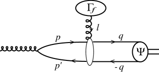
FIG. 3.: High $p_{\perp}$ quarkonium production via gluon fragmentation. The $Q\bar{Q}$ pair rescatters on the comoving color field $\Gamma_{f}$ before forming quarkonium.

A schematic view of our model is shown in Fig. 3 for ${}^{3}P_{J}$ quarkonia (which require a single rescattering). A high $p_{\perp}$ transverse gluon (typically produced in a process like $gg\to gg$, which does not concern us here) fragments into a heavy $Q\bar{Q}$ pair. The pair rescatters from an external field $\Gamma_{f}$ of hardness $\mu_{f}$ similar to the scale $\mu$ of Eq. (4) and forms a quarkonium bound state. The amplitude of the fragmentation process is a convolution, analogous to Eq. (LABEL:prodampl), of the quark pair wave function $\Phi_{f,{\lambda\bar{\lambda}}}^{[8]}$, the rescattering kernel ${\cal R}_{{\lambda\bar{\lambda}},{\sigma\bar{\sigma}}}(\mathchoice{{\hbox{\boldmath$\displaystyle\ell$}}}{{\hbox{\boldmath$\textstyle\ell$}}}{{\hbox{\boldmath$\scriptstyle\ell$}}}{{\hbox{\boldmath$\scriptscriptstyle\ell$}}},\mathchoice{{\hbox{\boldmath$\displaystyle p$}}}{{\hbox{\boldmath$\textstyle p$}}}{{\hbox{\boldmath$\scriptstyle p$}}}{{\hbox{\boldmath$\scriptscriptstyle p$}}},\mathchoice{{\hbox{\boldmath$\displaystyle q$}}}{{\hbox{\boldmath$\textstyle q$}}}{{\hbox{\boldmath$\scriptstyle q$}}}{{\hbox{\boldmath$\scriptscriptstyle q$}}})$ given by Eqs. (8) and (2), and the quarkonium wave function $\Psi_{\sigma\bar{\sigma}}^{L_{z}S_{z}}(\mathchoice{{\hbox{\boldmath$\displaystyle q$}}}{{\hbox{\boldmath$\textstyle q$}}}{{\hbox{\boldmath$\scriptstyle q$}}}{{\hbox{\boldmath$\scriptscriptstyle q$}}})$ of Eq. (9). As in the low $p_{\perp}$ situation, the heavy quarks are assumed to be on-shell before and after the rescattering.

The wave function $\Phi_{f,{\lambda\bar{\lambda}}}^{[8]}$ of the pair in the quarkonium rest frame is

$$\Phi_{f,{\lambda\bar{\lambda}}}^{[8]}=\chi_{\lambda}^{\dagger}\,\tilde{\Phi}_{f}^{[8]}\,\chi_{-\bar{\lambda}}=g\,T^{a}_{ij}\,{\bar{u}}_{\lambda}(\mathchoice{{\hbox{\boldmath$\displaystyle p$}}}{{\hbox{\boldmath$\textstyle p$}}}{{\hbox{\boldmath$\scriptstyle p$}}}{{\hbox{\boldmath$\scriptscriptstyle p$}}})\parbox[b]{6.00006pt}{$e$}\parbox[b]{5.50003pt}{ \raisebox{-0.86108pt}{$/$}}(\lambda_{g}){v}_{\bar{\lambda}}(\mathchoice{{\hbox{\boldmath$\displaystyle p$}}}{{\hbox{\boldmath$\textstyle p$}}}{{\hbox{\boldmath$\scriptstyle p$}}}{{\hbox{\boldmath$\scriptscriptstyle p$}}}^{\prime})$$ (38)

$$\tilde{\Phi}_{f}^{[8]}(\mathchoice{{\hbox{\boldmath$\displaystyle p$}}}{{\hbox{\boldmath$\textstyle p$}}}{{\hbox{\boldmath$\scriptstyle p$}}}{{\hbox{\boldmath$\scriptscriptstyle p$}}},\mathchoice{{\hbox{\boldmath$\displaystyle p$}}}{{\hbox{\boldmath$\textstyle p$}}}{{\hbox{\boldmath$\scriptstyle p$}}}{{\hbox{\boldmath$\scriptscriptstyle p$}}}^{\prime})=-2mg\,T^{a}_{ij}\left\{{\hat{e}}(\lambda_{g})+\frac{{\hat{p}}}{2m}\,{\hat{e}}(\lambda_{g})\,\frac{{\hat{p}}^{\prime}}{2m}\right\}$$ (39)

Here $a$, $i$, $j$ are the color indices of the gluon and quarks and $\mathchoice{{\hbox{\boldmath$\displaystyle e$}}}{{\hbox{\boldmath$\textstyle e$}}}{{\hbox{\boldmath$\scriptstyle e$}}}{{\hbox{\boldmath$\scriptscriptstyle e$}}}(\lambda_{g})$ is the polarization vector of the fragmenting gluon. For the range $p_{\perp}\gg m$ that we are considering the gluon is quasi-real and hence transversely polarized ($\lambda_{g}=\pm 1$) relative to its direction in the laboratory frame. An expansion in the small ratios $\mathchoice{{\hbox{\boldmath$\displaystyle p$}}}{{\hbox{\boldmath$\textstyle p$}}}{{\hbox{\boldmath$\scriptstyle p$}}}{{\hbox{\boldmath$\scriptscriptstyle p$}}}/m$, $\mathchoice{{\hbox{\boldmath$\displaystyle p$}}}{{\hbox{\boldmath$\textstyle p$}}}{{\hbox{\boldmath$\scriptstyle p$}}}{{\hbox{\boldmath$\scriptscriptstyle p$}}}^{\prime}/m$ has been made in Eq. (39).

B Production of ${}^{3}S_{1}$ states

Two rescatterings are needed to produce ${}^{3}S_{1}$ states via gluon fragmentation, see Fig. 4. The fragmentation amplitude ${\cal M}_{f}$ can thus be expressed as a convolution similar to (13), with two rescattering factors ${\cal R}$. Only the first term in the $Q\bar{Q}$ wave function (39), corresponding to a gluon fragmenting into a $Q\bar{Q}$ pair with $L=0$, actually contributes to $S$-wave production.

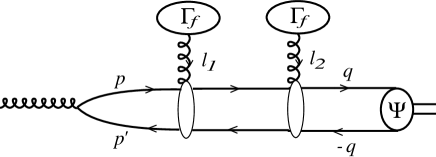
FIG. 4.: High $p_{\perp}$ ${}^{3}S_{1}$ production in the rescattering scenario (four Feynman diagrams).

We find for the ${}^{3}S_{1}$ production amplitude

$$M_{f}(^{3}S_{1},S_{z})=\frac{-mgR_{0}}{\sqrt{6\pi m}}$$ (40)

$$\times\left\{\right. {\rm Tr} \left.\left[a\,b_{2}\,b_{1}\right]{\rm Tr}\left[{\hat{e}}(S_{z})^{*}\tilde{\cal R}^{Q}(\mathchoice{{\hbox{\boldmath$\displaystyle\ell$}}}{{\hbox{\boldmath$\textstyle\ell$}}}{{\hbox{\boldmath$\scriptstyle\ell$}}}{{\hbox{\boldmath$\scriptscriptstyle\ell$}}}_{2},\mathchoice{{\hbox{\boldmath$\displaystyle 0$}}}{{\hbox{\boldmath$\textstyle 0$}}}{{\hbox{\boldmath$\scriptstyle 0$}}}{{\hbox{\boldmath$\scriptscriptstyle 0$}}})\tilde{\cal R}^{Q}(\mathchoice{{\hbox{\boldmath$\displaystyle\ell$}}}{{\hbox{\boldmath$\textstyle\ell$}}}{{\hbox{\boldmath$\scriptstyle\ell$}}}{{\hbox{\boldmath$\scriptscriptstyle\ell$}}}_{1},-\mathchoice{{\hbox{\boldmath$\displaystyle\ell$}}}{{\hbox{\boldmath$\textstyle\ell$}}}{{\hbox{\boldmath$\scriptstyle\ell$}}}{{\hbox{\boldmath$\scriptscriptstyle\ell$}}}_{2}){\hat{e}}(\lambda_{g})\right]\right.$$ (41)

$$+\left.\right. {\rm Tr} \left.\left[a\,b_{2}\,b_{1}\right]{\rm Tr}\left[\tilde{\cal R}^{\bar{Q}}(\mathchoice{{\hbox{\boldmath$\displaystyle\ell$}}}{{\hbox{\boldmath$\textstyle\ell$}}}{{\hbox{\boldmath$\scriptstyle\ell$}}}{{\hbox{\boldmath$\scriptscriptstyle\ell$}}}_{2},\mathchoice{{\hbox{\boldmath$\displaystyle 0$}}}{{\hbox{\boldmath$\textstyle 0$}}}{{\hbox{\boldmath$\scriptstyle 0$}}}{{\hbox{\boldmath$\scriptscriptstyle 0$}}}){\hat{e}}(S_{z})^{*}\tilde{\cal R}^{Q}(\mathchoice{{\hbox{\boldmath$\displaystyle\ell$}}}{{\hbox{\boldmath$\textstyle\ell$}}}{{\hbox{\boldmath$\scriptstyle\ell$}}}{{\hbox{\boldmath$\scriptscriptstyle\ell$}}}_{1},\mathchoice{{\hbox{\boldmath$\displaystyle 0$}}}{{\hbox{\boldmath$\textstyle 0$}}}{{\hbox{\boldmath$\scriptstyle 0$}}}{{\hbox{\boldmath$\scriptscriptstyle 0$}}}){\hat{e}}(\lambda_{g})\right]\right.$$ (42)

$$+\left.\right. {\rm Tr} \left.\left[a\,b_{1}\,b_{2}\right]{\rm Tr}\left[{\hat{e}}(S_{z})^{*}\tilde{\cal R}^{Q}(\mathchoice{{\hbox{\boldmath$\displaystyle\ell$}}}{{\hbox{\boldmath$\textstyle\ell$}}}{{\hbox{\boldmath$\scriptstyle\ell$}}}{{\hbox{\boldmath$\scriptscriptstyle\ell$}}}_{2},\mathchoice{{\hbox{\boldmath$\displaystyle 0$}}}{{\hbox{\boldmath$\textstyle 0$}}}{{\hbox{\boldmath$\scriptstyle 0$}}}{{\hbox{\boldmath$\scriptscriptstyle 0$}}}){\hat{e}}(\lambda_{g})\tilde{\cal R}^{\bar{Q}}(\mathchoice{{\hbox{\boldmath$\displaystyle\ell$}}}{{\hbox{\boldmath$\textstyle\ell$}}}{{\hbox{\boldmath$\scriptstyle\ell$}}}{{\hbox{\boldmath$\scriptscriptstyle\ell$}}}_{1},\mathchoice{{\hbox{\boldmath$\displaystyle 0$}}}{{\hbox{\boldmath$\textstyle 0$}}}{{\hbox{\boldmath$\scriptstyle 0$}}}{{\hbox{\boldmath$\scriptscriptstyle 0$}}})\right]\right.$$ (43)

$$+\left.\right. {\rm Tr} \left.\left[a\,b_{1}\,b_{2}\right]{\rm Tr}\left[\tilde{\cal R}^{\bar{Q}}(\mathchoice{{\hbox{\boldmath$\displaystyle\ell$}}}{{\hbox{\boldmath$\textstyle\ell$}}}{{\hbox{\boldmath$\scriptstyle\ell$}}}{{\hbox{\boldmath$\scriptscriptstyle\ell$}}}_{2},\mathchoice{{\hbox{\boldmath$\displaystyle 0$}}}{{\hbox{\boldmath$\textstyle 0$}}}{{\hbox{\boldmath$\scriptstyle 0$}}}{{\hbox{\boldmath$\scriptscriptstyle 0$}}}){\hat{e}}(S_{z})^{*}{\hat{e}}(\lambda_{g})\tilde{\cal R}^{\bar{Q}}(\mathchoice{{\hbox{\boldmath$\displaystyle\ell$}}}{{\hbox{\boldmath$\textstyle\ell$}}}{{\hbox{\boldmath$\scriptstyle\ell$}}}{{\hbox{\boldmath$\scriptscriptstyle\ell$}}}_{1},-\mathchoice{{\hbox{\boldmath$\displaystyle\ell$}}}{{\hbox{\boldmath$\textstyle\ell$}}}{{\hbox{\boldmath$\scriptstyle\ell$}}}{{\hbox{\boldmath$\scriptscriptstyle\ell$}}}_{2})\right]\right\}$$ (44)

where $b_{1}$, $b_{2}$ are the color indices of the two rescattering gluons and ${\rm Tr}\left[a\,b_{1}\,b_{2}\right]$ is a shorthand notation for ${\rm Tr}\left[T^{a}T^{b_{1}}T^{b_{2}}\right]$. The four terms in (40) correspond to the four Feynman diagrams implied in Fig. 4. Using (2) leads to the surprisingly simple result

$${\cal M}_{f}(^{3}S_{1},S_{z})=\frac{-R_{0}g^{3}}{2\sqrt{6\pi m^{3}}}\,d_{ab_{1}b_{2}}\mathchoice{{\hbox{\boldmath$\displaystyle G$}}}{{\hbox{\boldmath$\textstyle G$}}}{{\hbox{\boldmath$\scriptstyle G$}}}{{\hbox{\boldmath$\scriptscriptstyle G$}}}_{1}\cdot\mathchoice{{\hbox{\boldmath$\displaystyle e$}}}{{\hbox{\boldmath$\textstyle e$}}}{{\hbox{\boldmath$\scriptstyle e$}}}{{\hbox{\boldmath$\scriptscriptstyle e$}}}(\lambda_{g})\,\mathchoice{{\hbox{\boldmath$\displaystyle G$}}}{{\hbox{\boldmath$\textstyle G$}}}{{\hbox{\boldmath$\scriptstyle G$}}}{{\hbox{\boldmath$\scriptscriptstyle G$}}}_{2}\cdot\mathchoice{{\hbox{\boldmath$\displaystyle e$}}}{{\hbox{\boldmath$\textstyle e$}}}{{\hbox{\boldmath$\scriptstyle e$}}}{{\hbox{\boldmath$\scriptscriptstyle e$}}}(S_{z})^{*}$$ (46)

where $\mathchoice{{\hbox{\boldmath$\displaystyle G$}}}{{\hbox{\boldmath$\textstyle G$}}}{{\hbox{\boldmath$\scriptstyle G$}}}{{\hbox{\boldmath$\scriptscriptstyle G$}}}_{i}=\mathchoice{{\hbox{\boldmath$\displaystyle\Gamma$}}}{{\hbox{\boldmath$\textstyle\Gamma$}}}{{\hbox{\boldmath$\scriptstyle\Gamma$}}}{{\hbox{\boldmath$\scriptscriptstyle\Gamma$}}}_{f}(\mathchoice{{\hbox{\boldmath$\displaystyle\ell$}}}{{\hbox{\boldmath$\textstyle\ell$}}}{{\hbox{\boldmath$\scriptstyle\ell$}}}{{\hbox{\boldmath$\scriptscriptstyle\ell$}}}_{i})\times\mathchoice{{\hbox{\boldmath$\displaystyle\ell$}}}{{\hbox{\boldmath$\textstyle\ell$}}}{{\hbox{\boldmath$\scriptstyle\ell$}}}{{\hbox{\boldmath$\scriptscriptstyle\ell$}}}_{i}$. Note that (46) is independent of $\Gamma_{f}^{0}$. Only transverse gluons in the comoving gluon field contribute to ${}^{3}S_{1}$ quarkonium production at high $p_{\perp}$.

The expression (46) trivially satisfies the gauge invariance requirement ${\cal M}_{f}(\Gamma_{f}^{\mu}(\ell_{i})\to\ell_{i}^{\mu})=0$. Since the quarks are treated as being on-shell, each Feynman diagram contributing to the production amplitude separately satisfies current conservation. However, in order to keep track of gauge invariance when combining the different kernels $\cal{R}$, one must pay attention to their $\ell^{0}$-dependence. For instance the value of $\ell_{1}^{0}$ in $\tilde{\cal R}^{Q,\bar{Q}}(\mathchoice{{\hbox{\boldmath$\displaystyle\ell$}}}{{\hbox{\boldmath$\textstyle\ell$}}}{{\hbox{\boldmath$\scriptstyle\ell$}}}{{\hbox{\boldmath$\scriptscriptstyle\ell$}}}_{1},-\mathchoice{{\hbox{\boldmath$\displaystyle\ell$}}}{{\hbox{\boldmath$\textstyle\ell$}}}{{\hbox{\boldmath$\scriptstyle\ell$}}}{{\hbox{\boldmath$\scriptscriptstyle\ell$}}}_{2})$ differs from that in $\tilde{\cal R}^{Q,\bar{Q}}(\mathchoice{{\hbox{\boldmath$\displaystyle\ell$}}}{{\hbox{\boldmath$\textstyle\ell$}}}{{\hbox{\boldmath$\scriptstyle\ell$}}}{{\hbox{\boldmath$\scriptscriptstyle\ell$}}}_{1},\mathchoice{{\hbox{\boldmath$\displaystyle 0$}}}{{\hbox{\boldmath$\textstyle 0$}}}{{\hbox{\boldmath$\scriptstyle 0$}}}{{\hbox{\boldmath$\scriptscriptstyle 0$}}})$ by an amount $\delta\ell_{1}^{0}=-\mathchoice{{\hbox{\boldmath$\displaystyle\ell$}}}{{\hbox{\boldmath$\textstyle\ell$}}}{{\hbox{\boldmath$\scriptstyle\ell$}}}{{\hbox{\boldmath$\scriptscriptstyle\ell$}}}_{1}\cdot\mathchoice{{\hbox{\boldmath$\displaystyle\ell$}}}{{\hbox{\boldmath$\textstyle\ell$}}}{{\hbox{\boldmath$\scriptstyle\ell$}}}{{\hbox{\boldmath$\scriptscriptstyle\ell$}}}_{2}/m$. Now $\Gamma_{f}^{\mu}(\ell_{1}^{0},\mathchoice{{\hbox{\boldmath$\displaystyle\ell$}}}{{\hbox{\boldmath$\textstyle\ell$}}}{{\hbox{\boldmath$\scriptstyle\ell$}}}{{\hbox{\boldmath$\scriptscriptstyle\ell$}}}_{1})$ is related to $\Gamma_{f}^{\mu}(\ell_{1}^{0}+\delta\ell_{1}^{0},\mathchoice{{\hbox{\boldmath$\displaystyle\ell$}}}{{\hbox{\boldmath$\textstyle\ell$}}}{{\hbox{\boldmath$\scriptstyle\ell$}}}{{\hbox{\boldmath$\scriptscriptstyle\ell$}}}_{1})$ through a boost of velocity $\mathchoice{{\hbox{\boldmath$\displaystyle\beta$}}}{{\hbox{\boldmath$\textstyle\beta$}}}{{\hbox{\boldmath$\scriptstyle\beta$}}}{{\hbox{\boldmath$\scriptscriptstyle\beta$}}}=-\mathchoice{{\hbox{\boldmath$\displaystyle\ell$}}}{{\hbox{\boldmath$\textstyle\ell$}}}{{\hbox{\boldmath$\scriptstyle\ell$}}}{{\hbox{\boldmath$\scriptscriptstyle\ell$}}}_{2}/m$, $|\mathchoice{{\hbox{\boldmath$\displaystyle\beta$}}}{{\hbox{\boldmath$\textstyle\beta$}}}{{\hbox{\boldmath$\scriptstyle\beta$}}}{{\hbox{\boldmath$\scriptscriptstyle\beta$}}}|\ll 1$. One realizes that the vector $\mathchoice{{\hbox{\boldmath$\displaystyle\Gamma$}}}{{\hbox{\boldmath$\textstyle\Gamma$}}}{{\hbox{\boldmath$\scriptstyle\Gamma$}}}{{\hbox{\boldmath$\scriptscriptstyle\Gamma$}}}_{f}(\ell^{0},\mathchoice{{\hbox{\boldmath$\displaystyle\ell$}}}{{\hbox{\boldmath$\textstyle\ell$}}}{{\hbox{\boldmath$\scriptstyle\ell$}}}{{\hbox{\boldmath$\scriptscriptstyle\ell$}}})$ (and thus $\textstyle G$) is insensitive to this boost (at the level of our approximation) whereas the difference between $\Gamma_{f}^{0}(\ell_{1}^{0},\mathchoice{{\hbox{\boldmath$\displaystyle\ell$}}}{{\hbox{\boldmath$\textstyle\ell$}}}{{\hbox{\boldmath$\scriptstyle\ell$}}}{{\hbox{\boldmath$\scriptscriptstyle\ell$}}}_{1})$ and $\Gamma_{f}^{0}(\ell_{1}^{0}+\delta\ell_{1}^{0},\mathchoice{{\hbox{\boldmath$\displaystyle\ell$}}}{{\hbox{\boldmath$\textstyle\ell$}}}{{\hbox{\boldmath$\scriptstyle\ell$}}}{{\hbox{\boldmath$\scriptscriptstyle\ell$}}}_{1})$ is such that we get

$$\tilde{\cal R}^{Q,\bar{Q}}(\mathchoice{{\hbox{\boldmath$\displaystyle\ell$}}}{{\hbox{\boldmath$\textstyle\ell$}}}{{\hbox{\boldmath$\scriptstyle\ell$}}}{{\hbox{\boldmath$\scriptscriptstyle\ell$}}}_{1},-\mathchoice{{\hbox{\boldmath$\displaystyle\ell$}}}{{\hbox{\boldmath$\textstyle\ell$}}}{{\hbox{\boldmath$\scriptstyle\ell$}}}{{\hbox{\boldmath$\scriptscriptstyle\ell$}}}_{2})\simeq\tilde{\cal R}^{Q,\bar{Q}}(\mathchoice{{\hbox{\boldmath$\displaystyle\ell$}}}{{\hbox{\boldmath$\textstyle\ell$}}}{{\hbox{\boldmath$\scriptstyle\ell$}}}{{\hbox{\boldmath$\scriptscriptstyle\ell$}}}_{1},\mathchoice{{\hbox{\boldmath$\displaystyle 0$}}}{{\hbox{\boldmath$\textstyle 0$}}}{{\hbox{\boldmath$\scriptstyle 0$}}}{{\hbox{\boldmath$\scriptscriptstyle 0$}}})$$ (47)

which gives the simple form (46) for ${\cal M}_{f}$.

In the $S$-wave production amplitude (46) the dependence in $\lambda_{g}$ and $S_{z}$ is factorized. No correlation appears between the fragmenting gluon and quarkonium polarizations. Consequently, assuming only that $\Gamma_{f}$ is isotropically distributed in the (comoving) $Q\bar{Q}$ pair rest frame we predict that directly produced ${}^{3}S_{1}$ quarkonia are unpolarized at high $p_{\perp}$. Contrary to the low $p_{\perp}$ situation, we do not now need to assume the dominance of transverse gluons in $\Gamma_{f}$. The preliminary CDF data [12] on high $p_{\perp}$ $\psi^{\prime}$ production seems to prefer a longitudinal polarization, but the statistics is insufficient for a definite conclusion.

The high $p_{\perp}$ cross section ratio $\sigma(\psi^{\prime})/\sigma(J/\psi)$ appears to be larger [7] than the nearly universal ratio measured in low $p_{\perp}$ hadroproduction [19, 20, 21],

$$\left.\frac{\sigma(\psi^{\prime})}{\sigma_{dir}(J/\psi)}\right)_{p_{\perp}\gg m}\simeq 0.4>\left.\frac{\sigma(\psi^{\prime})}{\sigma_{dir}(J/\psi)}\right)_{p_{\perp}\leq m}\simeq 0.24$$ (48)

This is in qualitative agreement with our result that the rescattering gluons are transverse and thus couple to the spin of the individual quarks. In low $p_{\perp}$ production the target gluon is longitudinal (in the target rest frame) and its coupling is proportional to the $Q\bar{Q}$ color dipole size $r_{\perp}$. The convolution (LABEL:prodampl) then probes the bound state wave function in relatively larger configurations, where the node in the $\psi^{\prime}$ wave function tends to decrease its contribution [22, 23]. This systematics carries over to diffractive photoproduction, where two longitudinal gluon exchanges give a factor $r_{\perp}^{2}$, and the corresponding ratio (48) is measured to be $\simeq 0.15$ [24].

C Production of ${}^{3}P_{J}$ states

In the case of high $p_{\perp}$ ${}^{3}P_{J}$ production, only one scattering is needed (see Fig. 3). The production amplitude is given by the expression (13) with $\tilde{\Phi}^{[8]}$ replaced by $\tilde{\Phi}_{f}^{[8]}$ of Eq. (3). We expand the curly bracket of (13) at $\mathchoice{{\hbox{\boldmath$\displaystyle q$}}}{{\hbox{\boldmath$\textstyle q$}}}{{\hbox{\boldmath$\scriptstyle q$}}}{{\hbox{\boldmath$\scriptscriptstyle q$}}}\to\mathchoice{{\hbox{\boldmath$\displaystyle 0$}}}{{\hbox{\boldmath$\textstyle 0$}}}{{\hbox{\boldmath$\scriptstyle 0$}}}{{\hbox{\boldmath$\scriptscriptstyle 0$}}}$ and use for $P$-wave states

$$\int\frac{d^{3}\mathchoice{{\hbox{\boldmath$\displaystyle q$}}}{{\hbox{\boldmath$\textstyle q$}}}{{\hbox{\boldmath$\scriptstyle q$}}}{{\hbox{\boldmath$\scriptscriptstyle q$}}}}{(2\pi)^{3}}\Psi_{1L_{z}}^{*}(\mathchoice{{\hbox{\boldmath$\displaystyle q$}}}{{\hbox{\boldmath$\textstyle q$}}}{{\hbox{\boldmath$\scriptstyle q$}}}{{\hbox{\boldmath$\scriptscriptstyle q$}}}) = 0$$ (50)

$$\int\frac{d^{3}\mathchoice{{\hbox{\boldmath$\displaystyle q$}}}{{\hbox{\boldmath$\textstyle q$}}}{{\hbox{\boldmath$\scriptstyle q$}}}{{\hbox{\boldmath$\scriptscriptstyle q$}}}}{(2\pi)^{3}}\,\mathchoice{{\hbox{\boldmath$\displaystyle q$}}}{{\hbox{\boldmath$\textstyle q$}}}{{\hbox{\boldmath$\scriptstyle q$}}}{{\hbox{\boldmath$\scriptscriptstyle q$}}}\Psi_{1L_{z}}^{*}(\mathchoice{{\hbox{\boldmath$\displaystyle q$}}}{{\hbox{\boldmath$\textstyle q$}}}{{\hbox{\boldmath$\scriptstyle q$}}}{{\hbox{\boldmath$\scriptscriptstyle q$}}}) = i\sqrt{\frac{3}{4\pi m}}{R_{1}}^{\prime}\mathchoice{{\hbox{\boldmath$\displaystyle e$}}}{{\hbox{\boldmath$\textstyle e$}}}{{\hbox{\boldmath$\scriptstyle e$}}}{{\hbox{\boldmath$\scriptscriptstyle e$}}}(L_{z})^{*}$$ (51)

where ${R_{1}}^{\prime}$ is the derivative of the $P$-wave function at the origin. In the small $\textstyle q$ expansion the linear terms in $\textstyle q$ cannot arise from the rescattering kernel $\tilde{\cal R}$ because of the gauge invariance property mentioned in the preceding subsection. Recalling (47) with $\mathchoice{{\hbox{\boldmath$\displaystyle\ell$}}}{{\hbox{\boldmath$\textstyle\ell$}}}{{\hbox{\boldmath$\scriptstyle\ell$}}}{{\hbox{\boldmath$\scriptscriptstyle\ell$}}}_{2}$ replaced by $-\mathchoice{{\hbox{\boldmath$\displaystyle q$}}}{{\hbox{\boldmath$\textstyle q$}}}{{\hbox{\boldmath$\scriptstyle q$}}}{{\hbox{\boldmath$\scriptscriptstyle q$}}}$, one indeed sees that $\tilde{\cal R}^{Q}(\mathchoice{{\hbox{\boldmath$\displaystyle\ell$}}}{{\hbox{\boldmath$\textstyle\ell$}}}{{\hbox{\boldmath$\scriptstyle\ell$}}}{{\hbox{\boldmath$\scriptscriptstyle\ell$}}},\mathchoice{{\hbox{\boldmath$\displaystyle q$}}}{{\hbox{\boldmath$\textstyle q$}}}{{\hbox{\boldmath$\scriptstyle q$}}}{{\hbox{\boldmath$\scriptscriptstyle q$}}})$ is actually independent of $\textstyle q$. This means that the final orbital angular momentum of the $Q\bar{Q}$ pair $L=1$ must be fixed before the scattering, via the $L=1$ part of the $g\to Q\bar{Q}$ wave function $\tilde{\Phi}_{f}^{[8]}$. This statement remains true for any number of rescatterings. Thus only the second term of (39) contributes to $P$-wave production. Inserting (17) and (39) in (13) we arrive at

$${\cal M}_{f}(^{3}P_{J},J_{z}) = \frac{-g^{2}R_{1}^{\prime}/m}{4\sqrt{2\pi m^{3}}}\delta^{a}_{b}A^{\alpha\beta}B^{\alpha\beta,ij}\mathchoice{{\hbox{\boldmath$\displaystyle e$}}}{{\hbox{\boldmath$\textstyle e$}}}{{\hbox{\boldmath$\scriptstyle e$}}}{{\hbox{\boldmath$\scriptscriptstyle e$}}}^{i}(\lambda_{g}){{\rm\bf{H}}}^{j}$$ (53)

$$A^{\alpha\beta} = \sum_{L_{z}S_{z}}\langle LL_{z};SS_{z}|JJ_{z}\rangle\mathchoice{{\hbox{\boldmath$\displaystyle e$}}}{{\hbox{\boldmath$\textstyle e$}}}{{\hbox{\boldmath$\scriptstyle e$}}}{{\hbox{\boldmath$\scriptscriptstyle e$}}}^{\alpha}(L_{z})^{*}\mathchoice{{\hbox{\boldmath$\displaystyle e$}}}{{\hbox{\boldmath$\textstyle e$}}}{{\hbox{\boldmath$\scriptstyle e$}}}{{\hbox{\boldmath$\scriptscriptstyle e$}}}^{\beta}(S_{z})^{*}$$ (54)

$$B^{\alpha\beta,ij} = \delta_{i}^{j}\delta_{\alpha}^{\beta}+\delta_{i}^{\alpha}\delta_{j}^{\beta}-\delta_{i}^{\beta}\delta_{j}^{\alpha}$$ (55)

$${{\rm\bf{H}}} = \mathchoice{{\hbox{\boldmath$\displaystyle\ell$}}}{{\hbox{\boldmath$\textstyle\ell$}}}{{\hbox{\boldmath$\scriptstyle\ell$}}}{{\hbox{\boldmath$\scriptscriptstyle\ell$}}}^{2}\mathchoice{{\hbox{\boldmath$\displaystyle\Gamma$}}}{{\hbox{\boldmath$\textstyle\Gamma$}}}{{\hbox{\boldmath$\scriptstyle\Gamma$}}}{{\hbox{\boldmath$\scriptscriptstyle\Gamma$}}}_{f}+2m\Gamma_{f}^{0}\mathchoice{{\hbox{\boldmath$\displaystyle\ell$}}}{{\hbox{\boldmath$\textstyle\ell$}}}{{\hbox{\boldmath$\scriptstyle\ell$}}}{{\hbox{\boldmath$\scriptscriptstyle\ell$}}}$$ (56)

where $B^{\alpha\beta,ij}$ arises from the trace of four Pauli matrices. Using the form of the tensor $A^{\alpha\beta}$ given in [25] we get

$${\cal M}_{f}( {}^{3}P_{J} ,J_{z})=\frac{g^{2}\sqrt{3}R_{1}^{\prime}/m}{4\sqrt{2\pi m^{3}}}\delta^{a}_{b}$$ (57)

$$\times \left\{\begin{array}[]{cc}\mathchoice{{\hbox{\boldmath$\displaystyle e$}}}{{\hbox{\boldmath$\textstyle e$}}}{{\hbox{\boldmath$\scriptstyle e$}}}{{\hbox{\boldmath$\scriptscriptstyle e$}}}(\lambda_{g})\cdot{{\rm\bf{H}}}&(J=0)\\ i\sqrt{\frac{2}{3}}\mathchoice{{\hbox{\boldmath$\displaystyle e$}}}{{\hbox{\boldmath$\textstyle e$}}}{{\hbox{\boldmath$\scriptstyle e$}}}{{\hbox{\boldmath$\scriptscriptstyle e$}}}(\lambda_{g})\cdot({{\rm\bf{H}}}\times\mathchoice{{\hbox{\boldmath$\displaystyle e$}}}{{\hbox{\boldmath$\textstyle e$}}}{{\hbox{\boldmath$\scriptstyle e$}}}{{\hbox{\boldmath$\scriptscriptstyle e$}}}(J_{z})^{*})&(J=1)\\ 0&(J=2)\end{array}\right.$$ (61)

The amplitude vanishes for $J=2$ since in this case $A^{\alpha\beta}$ is symmetric and $A^{\alpha}_{\alpha}=0$. Experimentally $\sigma(\chi_{2})\simeq\sigma(\chi_{1})$ at large $p_{\perp}$ [26]. The cross section for $\chi_{2}$ production should be generated either by more than one rescattering in our scenario or by the CSM (or COM) mechanism of gluon emission.

To conclude this section we give our prediction for the $\chi_{1}$ polarization at large $p_{\perp}$ and discuss its dependence on the rescattering field $\Gamma_{f}$.

The high $p_{\perp}$ fragmenting gluon being quasi transverse we have from (61)

$$|{\cal M}_{f}^{\chi_{1}}(J_{z})|^{2}\propto|({{\rm\bf{H}}}\times\mathchoice{{\hbox{\boldmath$\displaystyle e$}}}{{\hbox{\boldmath$\textstyle e$}}}{{\hbox{\boldmath$\scriptstyle e$}}}{{\hbox{\boldmath$\scriptscriptstyle e$}}}(J_{z})^{*})_{\perp}|^{2}=\left\{\begin{array}[]{cc}|{{\rm\bf{H}}}_{\perp}|^{2}&(J_{z}=0)\\ |{{\rm\bf{H}}}^{z}|^{2}&(J_{z}=\pm 1)\\ \end{array}\right.$$ (62)

where the direction of the high $p_{\perp}$ gluon in the laboratory frame is chosen as the reference axis. For a general field $\Gamma_{f}$, the $\chi_{1}$ polarization depends on the relative importance of the two terms contributing to the vector ${{\rm\bf{H}}}$ given in (56). However, assuming that $\textstyle\ell$ is isotropically distributed, we find the same result for the $\chi_{1}$ polarization parameter

$$\lambda_{\chi_{1}}=\frac{\sigma(J_{z}=+1)-\sigma(J_{z}=0)}{\sigma(J_{z}=+1)+\sigma(J_{z}=0)}=-\frac{1}{3}$$ (63)

in the two following extreme cases:

• $\Gamma_{f}$ contains only transverse gluons (the first term of ${{\rm\bf{H}}}$ dominates) and is modelled by the ansatz (33) used at low $p_{\perp}$.

• $\Gamma_{f}$ is purely longitudinal (the second term of ${{\rm\bf{H}}}$ dominates).

Thus, rather independently of the form of $\Gamma_{f}$, we predict the $\chi_{1}$ yield to be longitudinally polarized if the rescattering scenario dominates $\chi_{1}$ production at high $p_{\perp}$.

IV Summary and discussion

We presented an extension of the approach of I to high $p_{\perp}$ quarkonium production. As in our previous work, we assumed the presence of rescattering between the heavy quark pair and a comoving color field, and found that such a scenario qualitatively agrees with the low and high $p_{\perp}$ data. We summarize here our main results and predictions.

At low $p_{\perp}$, the rescattering mechanism applies only to hadroproduction, not to photoproduction (in the photon fragmentation region). In order to agree with the observed non-polarization of ${}^{3}S_{1}$ low $p_{\perp}$ hadroproduction, we assume the field $\Gamma$ created at low $p_{\perp}$ to contain dominantly transversely polarized gluons. The $\sigma(\chi_{1})/\sigma(\chi_{2})$ ratio is found to be compatible with the measured value and our main predictions at low $p_{\perp}$ are:

• Direct $\chi_{1}$ production is transverse.

• $\sigma_{dir}(\chi_{2},J_{z}=0)/\sigma_{dir}(\chi_{2},J_{z}=\pm 1)=2/3$. In addition, we expect a significant CSM (no rescattering) contribution to $\sigma(\chi_{2})$, having $J_{z}=\pm 2$.

The comoving field $\Gamma_{f}$ arising from high $p_{\perp}$ gluon fragmentation is a priori different from the low $p_{\perp}$ field $\Gamma$. Our scenario is identical in high $p_{\perp}$ hadroproduction and high $p_{\perp}$ photoproduction, the $Q\bar{Q}$ pair originating from gluon fragmentation in both cases. Our predictions at large $p_{\perp}$ are:

• Direct ${}^{3}S_{1}$ production is unpolarized.

• Direct $\chi_{1}$ production contains a longitudinal component (Eq. (63)).

• $\chi_{2}$ is not produced via (a single) rescattering.

The prediction (iii) is consistent with the present CDF data on $\psi^{\prime}$ polarization [12], but higher statistics is needed for a definite conclusion. Only transverse gluon rescattering contributes to ${}^{3}S_{1}$ production. This is in qualitative agreement with the measured hadroproduction ratio $\sigma(\psi^{\prime})/\sigma_{dir}(J/\psi)$ being smaller at low than at high $p_{\perp}$ (cf. Eq. (48)), and being even smaller in diffractive photoproduction.

All our results and predictions apply equally to the charmonium and bottomonium families.

We used several simplifying assumptions which we now discuss.

• We supposed the rescattering color field to be isotropically distributed in the $Q\bar{Q}$ rest frame. Our predictions on ratios and relative polarization rates depend on this assumption.

• We assumed the rescatterings to be perturbative. Thus only the minimal number of rescatterings required to produce a given bound state was considered. On the other hand the rescattering probability should be large enough for this mechanism to dominate the CSM $S$-wave and (low $p_{\perp}$) $\chi_{1}$ rates. Whether such a compromise holds is not obvious and will be studied in a future work.

• It is unlikely that the production amplitude is sensitive only to the quarkonium wave function (or its derivative) at the origin, at least for charmonium. This is particularly so for $P$-waves (see the discussion of $\sigma(\chi_{2})/\sigma(J/\psi)$ in I) and when ‘dipole’ factors of $r_{\perp}$ enhance larger wave function configurations [23].

REFERENCES

• [1] Work supported in part by the EU/TMR contract EBR FMRX-CT96-0008.
• [2] J. C. Collins, D. E. Soper and G. Sterman, in Perturbative QCD, ed. A.H. Mueller (World Scientific, 1989); G. Bodwin, Phys. Rev.  D31, 2616 (1985) and D34, 3932 (1986) (E); J. Qiu and G. Sterman, Nucl. Phys. B353, 105 (1991) and B353, 137 (1991).
• [3] J. H. Kühn, Phys. Lett. 89B, 385 (1980); C. H. Chang, Nucl. Phys. B172, 425 (1980); E. L. Berger and D. Jones, Phys. Rev.  D23, 1521 (1981); R. Baier and R. Rückl, Phys. Lett. 102B, 364 (1981) and Z. Phys. C19, 251 (1983); J. G. Körner, J. Cleymans, M. Karoda and G. J. Gounaris, Nucl. Phys. B204, 6 (1982).
• [4] M. Krämer, J. Zunft, J. Steegborn and P. M. Zerwas, Phys. Lett. B348, 657 (1995); M. Krämer, Nucl. Phys. B459, 3 (1996).
• [5] S. Aid et al. (H1 Collaboration), Nucl. Phys. B472, 3 (1996), hep-ex/9603005; J. Breitweg et al. (ZEUS Collaboration), Z. Phys. C76, 599 (1997), hep-ex/9708010.
• [6] E. Braaten, M. A. Doncheski, S. Fleming and M. L. Mangano, Phys. Lett. 333B, 548 (1994), hep-ph/9405407; M. W. Bailey (CDF Collaboration), FERMILAB-CONF-96-235-E, hep-ex/9608014; F. Abe et al. (CDF Collaboration), FERMILAB-PUB-97-024-E, Phys. Rev. Lett. 79, 572 (1997); S. Abachi et al. (DØ Collaboration), FERMILAB PUB-96/003-E, Phys. Lett. B370, 239 (1996).
• [7] A. Sansoni, Fermilab-Conf-95/263-E, Nuovo Cim. A109, 827 (1996) and Fermilab-Conf-96/221-E, Nucl. Phys. A610, 373c (1996).
• [8] G. T. Bodwin, E. Braaten and G. P. Lepage, Phys. Rev.  D51, 1125 (1995), Erratum ibid., D55, 5853 (1997), hep-ph/9407339.
• [9] E. Braaten and S. Fleming, Phys. Rev. Lett. 74, 3327 (1995), hep-ph/9411365; M. Cacciari, M. Greco, M. L. Mangano and A. Petrelli, Phys. Lett. B356, 553 (1995), hep-ph/9505379; P. Cho and A. K. Leibovich, Phys. Rev.  D53, 150 (1996), hep-ph/9505329 and Phys. Rev.  D53, 6203 (1996), hep-ph/9511315.
• [10] P. Hoyer and S. Peigné, Phys. Rev. D59:034011 (1999), hep-ph/9806424.
• [11] P. Hoyer, Nucl. Phys. Proc. Suppl. 75B 153 (1999), hep-ph/9809362
• [12] A. Ribon (CDF Collaboration), FERMILAB-CONF-99/161-E, Proceedings of the 13th ‘Rencontres de Physique de la Vallée d’Aoste’, La Thuile (March 1999);
R. Cropp (CDF Collaboration), FERMILAB-CONF-99/250-E, Proc. Int. Europhysics Conf. EPS-HEP 99, Tampere, Finland, (July 1999), hep-ex/9910003.
• [13] E. Braaten, B. A. Kniehl and J. Lee, hep-ph/9911436.
• [14] J. Badier et al. (NA3 Collaboration), Z. Phys. C20, 101 (1983).
• [15] C. Biino et al. , Phys. Rev. Lett. 58, 2523 (1987); C. Akerlof et al. (E537 Collaboration), Phys. Rev.  D48, 5067 (1993); A. Gribushin et al. (E672/E706 Collaborations) Phys. Rev.  D53, 4723 (1996); T. Alexopoulos et al. (E771 Collaboration), Phys. Rev.  D55, 3927 (1997).
• [16] J. G. Heinrich et al. , Phys. Rev.  D44, 1909 (1991).
• [17] T. Alexopoulos et al. (E771 Collaboration), hep-ex/9908010.
• [18] E. Braaten and T. C. Yuan, Phys. Rev. Lett. 71, 1673 (1993); E. Braaten, M. A. Doncheski, S. Fleming, M. L. Mangano, Phys. Lett. 333B, 548 (1994), hep-ph/9405407; E. Braaten, S. Fleming, Phys. Rev. Lett. 74, 3327 (1995), hep-ph/9411365.
• [19] M. Vänttinen, P. Hoyer, S. J. Brodsky and W.-K. Tang, Phys. Rev.  D51, 3332 (1995).
• [20] C. Lourenço, Nucl. Phys. A610, 552c (1996), hep-ph/9612222.
• [21] R. Gavai, D. Kharzeev, H. Satz, G. A. Schuler, K. Sridhar and R. Vogt, Int. J. Mod. Phys. A10, 3043 (1995), hep-ph/9502270.
• [22] B. Z. Kopeliovich and B. G. Zakharov, Phys. Rev.  D44, 3466 (1991); B. Z. Kopeliovich, J. Nemchik, N. N. Nikolaev and B. G. Zakharov, Phys. Lett. B309, 179 (1993), hep-ph/9305225.
• [23] P. Hoyer and S. Peigné, Phys. Rev. D61:031501 (2000), hep-ph/9909519.
• [24] U. Camerini et al, Phys. Rev. Lett. 35, 483 (1975);
C. Adloff et al.  (H1 Collaboration), Phys. Lett. B421, 385 (1998), hep-ex/9711012.
• [25] P. Cho and A. K. Leibovich, Phys. Rev.  D53, 150 (1996), hep-ph/9505329 and Phys. Rev.  D53, 6203 (1996), hep-ph/9511315.
• [26] F. Abe et al. (CDF Collaboration), FERMILAB-Conf-95/226-E and Phys. Rev. Lett. 79, 578 (1997)).