Pattern Formation in the Early Universe

Abstract

Systems that exhibit pattern formation are typically driven and dissipative. In the early universe, parametric resonance can drive explosive particle production called preheating. The fields that are populated then decay quantum mechanically if their particles are unstable. Thus, during preheating, a driven-dissipative system exists. We have shown previously that pattern formation can occur in two dimensions in a self-coupled inflaton system undergoing parametric resonance. In this paper, we provide evidence of pattern formation for more realistic initial conditions in both two and three dimensions. In the one-field case, we have the novel interpretation that these patterns can be thought of as a network of domain walls. We also show that the patterns are spatio-temporal, leading to a distinctive, but probably low-amplitude peak in the gravitational wave spectrum. In the context of a two-field model, we discuss putting power from resonance into patterns on cosmological scales, in particular to explain the observed excess power at $100h^{-1}$Mpc, but why this seems unlikely in the absence of a period of post-preheating inflation. Finally we note our model is similar to that of the decay of DCCs and therefore pattern formation may also occur at RHIC and LHC.

Fermilab Preprint: Pub-98/231-A       BROWN-HET-1201       Imperial/TP/99-0/006

]

I Introduction

Much recent work has been devoted to the topic of preheating in inflationary cosmology. Preheating is a stage of explosive particle production which results from the resonant driving of particle modes by an inflaton oscillating in its potential at the end of inflation [1, 2, 3].

In regions of parameter space where parametric resonance is effective, much of the energy of the inflaton is transferred to bands of resonant wave modes. This energy transfer is non-thermal and can lead to interesting non-equilibrium behavior. Two examples of the non-equilibrium effects that can be produced are non-thermal phase transitions [4, 5, 6, 7] and baryogenesis [8, 9, 10, 11]. The non-thermal phase transitions induced during preheating can sometimes lead to topological defect formation [12, 13, 14, 15], even at energies above the eventual final thermal temperature. Furthermore, non-linear evolution of the field when quantum decay of the resonantly produced particles is negligible leads to a chaotic power-law spectrum of density fluctuations [16, 17].

In a previous letter [19], we presented evidence for a new phenomenon that can arise from preheating: pattern formation. It has long been known that many condensed matter systems exhibit pattern formation. Examples of pattern forming systems which have been studied are ripples on sand dunes, cloud streets and a variety of other convective systems, chemical reaction-diffusion systems, stellar atmospheres and vibrated granular materials. All of these physical systems have two features in common. They are all driven in some manner, i.e. energy is input to the system, and they are all dissipative, usually being governed by diffusive equations of motion. Typically, patterns are formed in these systems in the weakly non-linear regime before the energy introduced into the system overwhelms the dissipative mechanism. Sometimes, patterns persist beyond the weakly non-linear regime as well.

At the end of inflation, the inflaton $\phi$ is homogeneous and, in most commonly studied models, oscillating about the minimum of its potential. This oscillation gives an effectively time-dependent mass to fields which are coupled to the inflaton, including fluctuations of the inflaton itself. The time-dependent mass drives exponential growth in particle number in certain bands of wave modes. However the fields into which the inflaton can decay resonantly are also unstable to quantum decay. For these reasons, at the end of inflation, we are considering fields which are driven, due to resonant particle creation, and also dissipative, due to quantum decay. In [19], we were able to show that pattern formation occurs in a chaotic inflationary model with a self-coupled inflaton in the weakly non-linear regime.

In this paper, we primarily consider a $\lambda\phi^{4}$ theory with the addition of a phenomenological decay term to mimic the inflaton’s quantum decay. This model without the decay term has been studied extensively in the literature[2, 3, 16, 18, 17, 20, 23], and a similar model including the decay term has also been studied [10].

In [19], we used restricted initial conditions. We only seeded the resonant band with small fluctuations of order $\sim 10^{-3}$ of $\langle\phi\rangle$, then simulated the field’s evolution. We found that the resonant modes interacted and formed patterns. Here we use initial conditions appropriate to the vacuum at the end of chaotic inflation. We also extend our study to a 3-dimensional volume. In [19], we did not point out the spatio-temporal nature of the patterns, which was not evident at the time due to an unfortunate coincidence in the form of the pattern at the timesteps at which we viewed the data. Here we note the spatio-temporal behavior. We also discuss resonance giving rise to patterns on cosmological scales.

The paper is ordered as follows: In section II, we present the model we are investigating. In section III, we discuss the initial conditions appropriate for the end of inflation. In sections IV, we present the results of our simulations in two and three spatial dimensions. In section V, we extend our analysis to the two-field case and discuss the possible implications of our results. This is followed by the conclusions.

II The $\lambda\phi^{4}$ Model with Phenomenological Damping

Our field equation in comoving coordinates is

$$\ddot{\phi}+3H\dot{\phi}+\gamma\dot{\phi}-\frac{1}{a^{2}}\nabla^{2}\phi+\lambda\phi^{3}=0$$ (1)

where $\gamma$ is a decay constant, $\lambda$ is the self-coupling of the field and $H\equiv\dot{a}/a$. We convert to conformal time $dt=a(\tau)d\tau$ and introduce the field $\varphi=a\phi$. Upon rescaling: $\tau\rightarrow\tau/\sqrt{\lambda}\varphi_{R}$, $x\rightarrow x/\sqrt{\lambda}\varphi_{R}$ and $\varphi\rightarrow\varphi\,\varphi_{R}$, where subscript $R$ denotes “at the start of reheating”, we obtain a new equation

$$\varphi^{\prime\prime}+a\Gamma\varphi^{\prime}-\nabla^{2}\varphi-(a^{\prime}\Gamma+\frac{a^{\prime\prime}}{a})\,\varphi+\varphi^{3}=0,$$ (2)

where $\Gamma=\gamma/\sqrt{\lambda}\varphi_{R}$. Further simplification is possible if we note that in $\lambda\phi^{4}$ theory, the averaged equation of state during preheating is that of radiation, therefore $a^{\prime\prime}\simeq 0$. We use $a=1+H_{R}\tau$.

It should be noted that pattern formation in the inflaton system is conceptually distinct from condensed matter systems for at least two reasons. First, the equations we study are wave equations with damping, not diffusive equations. Secondly, we expect wave patterns to be formed while the homogeneous mode decays, therefore pattern formation will be a temporary phenomenon, at least in the model above in which gravity is neglected. The driving in $\lambda\phi^{4}$ preheating comes from the large initial value of the inflaton at the end of inflation, causing the field to roll and oscillate in its potential. This should be considered in contrast to the typical condensed matter system, in which energy is introduced via boundary conditions (in a convective system) or by a vibrating bed (in a granular material system), and the energy input is essentially constant.

At the end of inflation, we may expand $\varphi$ about a homogeneous piece and then linearize Eq. (2). Let $\varphi(\tau,{\bf x})=\Phi(\tau)+\psi(\tau,{\bf{x}})$, where $\int\psi\,d^{3}x=0$. We obtain

$$\Phi^{\prime\prime}+\Phi^{3} = 0$$ (3)

$$\psi^{\prime\prime}_{\bf k}+a\Gamma\psi^{\prime}_{\bf k}+\left(k^{2}-a^{\prime}\Gamma+3\Phi^{2}(\tau)\right)\psi_{\bf k} = 0,$$ (4)

where we have taken the Fourier transform in the latter equation. The solution to Eq. (3) is $\Phi(\tau)=\mbox{cn}(\tau;1/\sqrt{2})$, and therefore, for $\Gamma=0$, Eq. (4) becomes a Lamé equation.

For $\Gamma=0$, the resonant modes lie in the interval[23]

$$\frac{3}{2}<k^{2}<\sqrt{3},$$ (5)

and have an amplitude of the form $\exp{(\mu_{k}\tau)}$, where $\mu_{k}$ is the characteristic exponent or Floquet index. It should be noted that the wavelengths of the resonant modes are of order the Hubble radius immediately after inflation.

For $\Gamma\neq 0$, we can introduce $\bar{\psi}=\psi\,\exp({1\over 2}\int a\Gamma d\tau)$ giving

$$\bar{\psi}^{\prime\prime}_{\bf k}+\left(k^{2}-{3\over 2}a^{\prime}\Gamma-{1\over 4}a^{2}\Gamma^{2}+3\Phi^{2}(\tau)\right)\bar{\psi}_{\bf k}=0.$$ (6)

Now the resonance band becomes time-varying. The modes which can be in resonance at any moment in time satisfy $\frac{3}{2}<k_{\mbox{{eff}}}^{2}<\sqrt{3}$, where

$$k^{2}_{\mbox{{eff}}}=k^{2}-{3\over 2}a^{\prime}\Gamma-{1\over 4}a^{2}\Gamma^{2}.$$ (7)

However the modes we are actually interested in are $\psi_{\bf k}/a$, and these will only grow for times $\tau\lesssim 4|\mu_{k}|/H_{R}\Gamma$. This is because we typically have $\Gamma\ll|\mu_{k}|<H_{R}\lesssim 1$ (in rescaled units). Thus, even in the absence of backreaction, a combination of the expansion of the universe and quantum mechanical decay of the inflaton serves to take the system out of resonance. During this time the values of $k^{2}$ in resonance go from being shifted upwards by an amount $\Gamma$ to an amount $4\mu_{k}^{2}$. Effectively this means the resonance band is smeared out in $k$-space.

While the above perturbative analysis is helpful it is suitable only for early times as resonance will soon take us away from the linear regime. The effect that we are trying to isolate is intrinsically non-linear so we now resort to numerical simulation of the field equation (2).

III Initial Conditions

The initial conditions for $\Phi$ are those of the end of slow-roll, which is normally supposed to be when $\ddot{a}=0$. It is sufficient for our purposes to set $\Phi(0)=1$ and $\Phi^{\prime}(0)=0$.

The fluctuations in the inflaton are quantum in origin. Super-Hubble modes exist which were generated during inflation and have remained fixed in amplitude after leaving the Hubble volume. However these modes do not undergo amplification in this model, so it is not important to quantify them precisely. Of more significance for us are the sub-Hubble modes at the end of inflation. At this time $\Gamma$ is in fact zero and it is appropriate to consider any field to be in the vacuum state. Then the initial conditions for the $\psi_{\bf k}$ are given by the usual results:

$$\psi_{\bf k}=\frac{1}{\sqrt{2\omega_{k}}}|A_{\bf k}|e^{2\pi ir_{\bf k}}\qquad\psi^{\prime}_{\bf k}=-i\omega_{k}\psi_{\bf k},$$ (8)

where $\omega_{k}^{2}=k^{2}+3\Phi(0)^{2}$, $A_{\bf k}$ is a number randomly taken from a Gaussian distribution with zero mean and unit variance, and $r_{\bf k}$ is a random number taken from the interval $[0,1]$.

IV Simulation Results

A Two dimensions

To simulate the evolution of the field, we discretize the spatial derivatives to fourth-order in $\Delta x$, and we use a leapfrog integrator which is accurate to second order in $\Delta t$.

Setting the box size to $256$ gridpoints per dimension and such that the resonant wave number in the box is $16$ is enough to give many different resonant modes in the box, but still have good resolution of the wave, so this is the box size we used. We use periodic boundary conditions.

We set out to identify the weakly non-linear regime. Khlebnikov and Tkachev [16] showed that, without the decay terms, the self-coupled inflaton system’s non-linear time evolution proceeds as follows: First, the resonant band amplitude grows. Next, when the amplitude in the resonant band is high enough for non-linear effects to become important, period doubling occurs and subsidiary peaks develop in the power spectrum. Further peaks then develop and the spectrum broadens and approaches an exponential spectrum. We tuned $\Gamma$ such that the amplitude of the resonant band grew, but little period doubling occurred. In this regime, only resonant mode wavelengths exist in the box and they interact with each other non-linearly.

In the expanding case, the increase of the effective damping coefficient $\Gamma_{\mbox{{eff}}}=a\Gamma$ with increasing scale factor $a$ makes it easier to keep the system in the weakly non-linear regime compared to the non-expanding case.

We found the smallest value for $\Gamma$ such that the system remained weakly non-linear was of order $10^{-5}$. This is two orders of magnitude smaller than that in the non-expanding case.

In Figure 1 we plot a superposition of the power spectrum at various times during a simulation with $\Gamma=5\times 10^{-5}$. It is possible to see that the system stays in the weakly non-linear regime for the entire simulation.

FIG. 1.: A superposition of power spectra taken from a simulation with $\Gamma=5\times 10^{-5}$. We plot the amplitude of the power spectra vs. wave number. Note that the period doubling modes are only weakly populated, indicating that the simulation is in the weakly non-linear regime.

When wave patterns form, the specific pattern which arises is due to the non-linear interaction of the wave modes. The amplitude of wave modes separated by different angles grows at different rates. Modes separated by angles with the fastest growing amplitudes dominate the solution and form the wave pattern.

It is also possible that patterns vary temporally. This is the situation we find in the $\lambda\phi^{4}$ model. What we see in both the expanding and non-expanding cases is that a pattern emerges from the fluctuation background, then the peaks and valleys begin to move relative to each other.

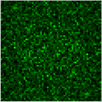
FIG. 2.: $t=0$. Initial conditions for a two-dimensional simulation with $\Gamma=5\times 10^{-5}$. The magnitude of $\tilde{\phi}(k_{x},k_{y})$, the Fourier transform of the inflaton, is indicated by the shading: brighter regions correspond to regions of larger amplitude. The zero mode has been deleted for plotting purposes, and the surrounding modes populated with vacuum amplitudes from Eq. 8. Only the region of interest is plotted.

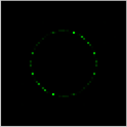
FIG. 3.: $t=840$. After resonance begins to boost the amplitude of the resonant mode. Notice the brightening (increasing amplitude) of the resonant modes.

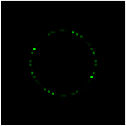
FIG. 4.: $t=1020$. The final wave pattern in Fourier space.

The temporal dependence is almost periodic. Peaks and troughs in the field energy align along one direction in a ripple-like pattern, then the pattern flips to align in a direction orthogonal to the original direction. We say the dependence is ‘almost’ periodic because the field flips back and forth, but the timing of the flips varies as the field evolves. This leads us to believe that, for instance, if there were a background driving field that gave constant energy input (as opposed to the decaying background in chaotic inflation) the flipping would be truly periodic.

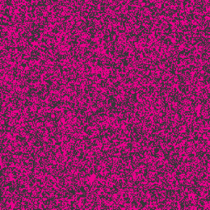
FIG. 5.: $t=0$. The initial conditions in configuration space. The inflaton $\phi(x,y)$ is plotted, again with brighter regions corresponding to larger values of $\phi$.

FIG. 6.: $t=840$. Wave pattern at intermediate time.

FIG. 7.: $t=1020$. Wave pattern at the end of the simulation.

In Figures 2, 3 and 4 we present snapshots of the evolution of the Fourier transform of the inflaton in two dimensions in an expanding universe. And in plots 5, 6 and 7 we present snapshots of the evolution of $\phi(x,y)$ in configuration space in two dimensions in an expanding universe. Notice the change in direction between the ripples in Figure 6 and 7.

In the expanding case (in contrast to the non-expanding case), the patterns are more clearly delineated and look less noisy. This is due to the fact that the field equation has an effective symmetry breaking potential and this leads to a restoring force on the fluctuations in $\varphi$. From Eq. (2) we deduce

$$V_{\mbox{{eff}}}(\varphi)={1\over 4}(\varphi^{2}-a^{\prime}\Gamma)^{2}$$ (9)

in a radiation dominated universe. The barrier height is $(a^{\prime}\Gamma/2)^{2}$ which is constant in time. Thus dissipation not only leads to an overall damping of the field, but also leads to degeneracy in the minima of the effective potential. This suggests a novel interpretation of pattern formation in this model: the pattern is actually a network of domain walls separated by the characteristic wavelength of the resonance. If $\Gamma$ increases then the barrier height increases, reflecting the fact that the non-linear coupling of the modes necessary for pattern formation is suppressed. On the other hand, for small $\Gamma$, the barrier is not high enough to prevent the field from probing both minima, and again patterns do not form. This is because the system has become strongly non-linear.

B Three dimensions

Using the same simulation techniques described above, we also find spatio-temporal pattern formation in three dimensions. We plot the field in configuration space in Figures 8, 9 and 10, again with $\Gamma=5\times 10^{-5}$. The behavior of these patterns is similar to those found in two dimensions: the pattern forms at the resonant wavelength, then the peaks and valleys begin to move with respect to each other. In these simulations, we set the physical box size such that there were eight resonant wavelengths per dimension in the box. Overall there were 64 gridpoints per dimension and we neglected expansion in these simulations.

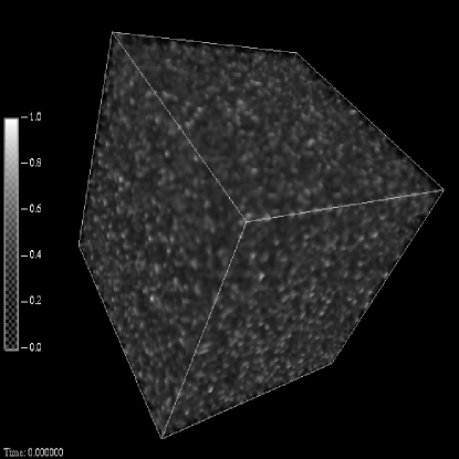
FIG. 8.: $t=0$. Initial conditions for a three-dimensional simulation with $\Gamma=5\times 10^{-5}$. Here $\phi(x,y,z)$ is plotted, again with brighter regions indicating larger field values.

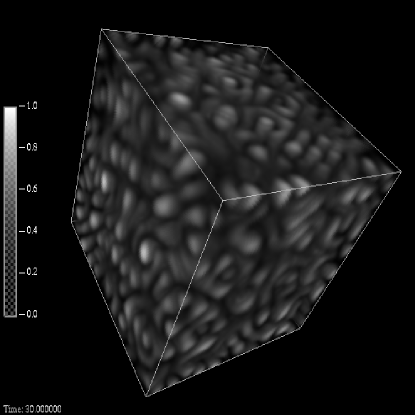
FIG. 9.: $t=100$. Wave pattern at intermediate time.

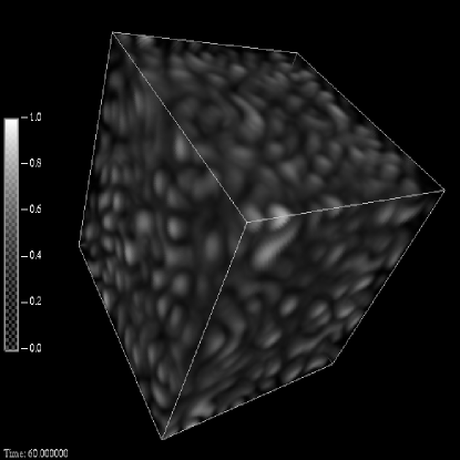
FIG. 10.: $t=300$. Wave pattern at the end of the simulation.

V Discussion

A Gravitational waves

Since the patterns that we see vary in time, we expect there to be a peak in the gravitational wave spectrum at the resonant frequency for preheating in the weakly non-linear regime. Similar peaks in the gravitational wave spectrum have been seen [24, 25] in simulations of undamped preheating. These peaks correspond to the resonant and period doubled frequencies. In the pattern forming regime, we expect to see similar peaks of lower amplitude, since the dissipative terms keep the resonant peak in our simulation at lower amplitude than the undamped system. The peak in the gravitational wave spectrum from pattern formation will be of smaller amplitude than that of the fully chaotic system but since the pattern has directionality, this might help in extracting a signal.

B Large scale structure formation

We would also like to discuss the possibility of patterns occurring on cosmological scales, since, if we could put resonant power at $100h^{-1}$Mpc, we would have an explanation for the observed excess power found at these scales [26]. Although such a scale is outside the Hubble radius at the end of inflation, recently a number of authors [27, 28, 29, 30, 31, 32, 33] have investigated the question of whether resonance can amplify modes with wavelength larger than the Hubble radius. It turns out that this is possible because of the large-scale (many Hubble volumes) coherence of the inflaton at the end of inflation; super-Hubble mode amplification can be thought of as down-scattering from the oscillating zero mode. However in the usual parameter region of some models [30, 31, 33], this amplification does not seriously affect the post-inflationary power spectrum. This is due to the fact that during inflation in these models, fluctuations in matter fields are suppressed by a factor of $a^{-3/2}$ compared to fluctuations in the inflaton. Therefore, during preheating, although super-Hubble modes are amplified, they cannot be amplified enough to be significant.

However consider the following model for preheating:

$$V={1\over 4}\lambda\phi^{4}+{1\over 2}g^{2}\phi^{2}\chi^{2}.$$ (10)

For $q\equiv g^{2}/\lambda\sim 1$, fluctuations in $\chi$ are not suppressed during inflation [32]. This is because the effective mass of $\chi$ is $g\phi$, and this is much less than $H$ during slow roll.

If we now suppose $\chi$ decays quantum mechanically into other particles, then we are led to a phenomenological equation of motion akin to Eq. (1)

$$\ddot{\chi}+3H\dot{\chi}+\gamma_{\chi}\dot{\chi}-{1\over a^{2}}\nabla^{2}\chi+g^{2}\phi^{2}\chi=0.$$ (11)

With the same simplifications used earlier, and introducing $X=\chi a\exp{({1\over 2}\int d\tau a\Gamma_{\chi}})$, we obtain the the following equation for the Fourier modes of $X$

$$X_{\bf k}^{\prime\prime}+\left(k^{2}_{\mbox{{eff}}}+q\Phi^{2}(\tau)\right)X_{\bf k}=0,$$ (12)

where now $k^{2}_{\mbox{{eff}}}=k^{2}-3a^{\prime}\Gamma_{\chi}/2-a^{2}\Gamma_{\chi}^{2}/4$. This differs essentially from Eq. (6) because of the appearance of $q$. A partial plot of the instability bands in the $(k^{2}_{\mbox{{eff}}},q)$-plane is shown in Figure 11. When $\Gamma_{\chi}\neq 0$ we have a new feature: for modes with $k$ small enough, we can have $k^{2}_{\mbox{{eff}}}<0$, i.e. the system can probe the lower half of instability plot.

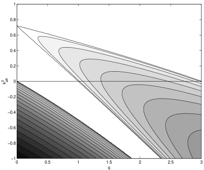
FIG. 11.: A portion of the instability plot for $q\simeq 1$ in Eq. (12). Darker shading indicates larger values of the characteristic exponent $\mu_{k}$. The narrow resonance band of Eq. (7) is not indicated.

If $k_{0}^{\mbox{{phy}}}$ is the physical scale today on which we want to have a feature in the power spectrum, then this corresponds to a co-moving mode $k_{R}$ at reheating such that

$${k_{R}\over{\cal H}_{R}}={k_{0}^{\mbox{{phy}}}\over H_{0}}{a_{0}\over a_{R}}{H_{0}\over H_{R}},$$ (13)

where ${\cal H}\equiv a^{\prime}/a=aH$. For a bump at $100h^{-1}$Mpc, we find we need $k_{R}/{\cal H}_{R}\sim 10^{-24}$. In terms of our dimensionless quantities this becomes $k_{R}\sim 10^{-24}$ which we want to be the principal wavelength in resonance. It follows that we have either $k^{2}_{\mbox{{eff}}}<0$ or $\Gamma_{\chi}\lesssim 10^{-48}$, but from our simulations the latter is ruled out because it will be too small to damp resonance and lead to pattern formation.

If we consider Figure 11 it is readily apparent that it will be difficult to introduce a feature at the required scale. For $q\ll 1$ we can have resonance at $k^{2}=10^{-24}$ but also, ruinously, at all scales down to $k=0$. Indeed the characteristic exponent becomes larger as $k$ gets smaller. We can avoid this problem for $q\gtrsim 1$ but only if $q$ is fine tuned to an unacceptable degree. In any case the resonance band is broad here (this problem is further exacerbated in our situation by the fact that quantum mechanical decay tends to smear the resonance bands) and peaks for modes with $k^{2}_{\mbox{{eff}}}>0$. Thus it is unlikely that super-Hubble mode amplification in this model can lead to a feature at $100h^{-1}$Mpc.

However we now mention that it may not be necessary to require such amplification in order to have an effect on large scale structure. It is possible that a post-preheating period of inflation[34, 4, 35] occurs (or even several) and this may bring sub-Hubble modes, previously amplified in narrow band resonance, up to scales appropriate for structure formation. The growth in the scale factor will also be larger if we imagine the inflaton decays into a large number of fields $\chi_{i}$, though we have not considered pattern formation in such models.

It should be noted that $\Gamma_{\chi}$ is not constrained in the same way $\Gamma_{\phi}$ is. The latter has to be small so that radiative corrections do not spoil the required flatness of the inflaton potential. In the rescaled units used here, it is not hard to show[36] that $\Gamma_{\phi}\lesssim 10^{-13}$, where we have taken $\lambda\simeq 10^{-13}$ which leads to the correct magnitude of density perturbations from inflation. Thus our earlier results were obtained with a $\Gamma$ which was too large to be physical. However the results should go through for the two-field model considered above.

C Patterns in heavy ion collisions

As a final comment, we would like to point out that the system of equations which we have investigated is similar to that for heavy ion collisions. It is hoped that in coming experiments at RHIC and LHC energies will be obtained which are in excess of the critical temperature for the QCD chiral phase transition. The situation may be modelled by an $O(4)$-symmetric theory for the scalar fields $\Phi=(\sigma,\vec{\pi})$[37], where one initially has $\langle\sigma\rangle=\langle\vec{\pi}\rangle=0$. Due to the expansion of the plasma, the temperature quickly falls below the critical temperature, the $O(4)$-symmetry is broken, and the system evolves to new equilibrium values $\langle\sigma\rangle\neq 0,\langle\vec{\pi}\rangle=0$. It is during this time that “disoriented chiral condensates” (DCCs), domains in which the pion field develops a non-zero expectation value in a certain direction, may be produced. The subsequent decay of a DCC gives rise to a characteristic signal in the detectors.

The important point for us is that during DCC decay, long-wavelength pion modes are resonantly amplified when $\sigma$ oscillates about the minimum of its effective potential[38]. Furthermore $\sigma$ decays via $\sigma\rightarrow 2\pi$ and it has been argued that this process can be modelled phenomenologically by the addition of a time-dependent friction term[39]. Although some questions remain concerning the applicability of such a term, it is intriguing that a driven-dissipative system exists for DCC decay. This suggests that patterns might turn up at RHIC and LHC. We are currently working on the experimental signatures of such events.

VI Conclusions

In this paper, we have presented new evidence that there is a pattern forming regime in a $\lambda\phi^{4}$ theory during preheating at the end of inflation. We have used vacuum initial conditions appropriate to sub-Hubble modes at the end of inflation. We have shown that patterns arise in both two- and three-dimensions, and that, in the one-field case, they may be thought of as a network of domain walls. Furthermore since the patterns vary spatio-temporally, gravitational waves will be produced. However, relative to the gravitational waves produced in an undamped model, their amplitude will be small, and therefore, unless the directionality of the pattern can aid in detection, extremely difficult to detect.

We have speculated on the possibility, in the context of a two-field model, of putting a resonant band at cosmological scales, in particular at $100h^{-1}$Mpc. We conclude that this is not feasible because it is impossible to amplify only the required modes. However this conclusion may change in a model which allows a subsequent period of inflation.

Finally, we point out that heavy ion collisions at RHIC and LHC may be another physical system which exhibits pattern forming behavior.

Acknowledgements

It is a pleasure to thank Ewan Stewart, Rocky Kolb, Robert Brandenberger, Bruce Bassett and Dan Boyanovsky for a number of useful discussions. We would also like to thank Bob Rosner and the Astrophysical Thermonuclear Flash Group at the University of Chicago for the use of their computational facilities. Much of this work was completed at Fermilab, supported by the DOE and the NASA grant NAG 5-7092, and at Brown under DOE contract DE-FG0291ER40688, Task A. A portion of the computational work in support of this research was performed at the Theoretical Physics Computing Facility at Brown University.

REFERENCES

- [1] J. Traschen & R. Brandenberger, Phys. Rev. D 42, (1990) 2491.
- [2] L. Kofman, A. Linde & A. Starobinsky, Phys. Rev. Lett. 73, (1994) 3195.
- [3] Y. Shtanov, J. Traschen & R. Brandenberger, Phys. Rev. D 51, (1995) 5438.
- [4] L. Kofman, A. Linde & A. Starobinsky, Phys. Rev. Lett. 76, (1996) 1011.
- [5] I. Tkachev, Phys. Lett. B 376, (1996) 35.
- [6] A. Riotto & I. Tkachev, Phys. Lett. B 385, (1996) 57.
- [7] S. Khlebnikov, L. Kofman, A. Linde & I. Tkachev, Phys. Rev. Lett. 81, (1998) 2012.
- [8] G. Anderson, A. Linde & A. Riotto, Phys. Rev. Lett. 77, (1996) 3716.
- [9] E. Kolb, A. Linde & A. Riotto, Phys. Rev. Lett. 77, (1996) 4290.
- [10] E. Kolb, A. Riotto & I. Tkachev, Phys. Lett. B 423, (1998) 348.
- [11] J. Garcia-Bellido, D. Grigorev, A. Kusenko & M. Shaposhnikov, Phys. Rev. D 60 (1999) 123504.
- [12] S. Kasuya & M. Kawasaki, Phys. Rev. D 56, (1997), 7597; S. Kasuya & M. Kawasaki, Phys. Rev. D 58, (1998) 083516; S. Kasuya & M. Kawasaki, hep-ph/9903324 (1999).
- [13] I. Tkachev, S. Khlebnikov, L. Kofman & A. Linde, Phys. Lett. B 440, (1998) 262.
- [14] M. Parry & A. Sornborger, Phys. Rev. D 60 (1999) 103504.
- [15] S. Digal, R. Ray, S. Sengupta & A. Srivastava, hep-ph/9911446 (1999).
- [16] S. Khlebnikov & I. Tkachev, Phys. Rev. Lett. 77, (1996) 219.
- [17] T. Prokopec & T. Roos, Phys. Rev. D 55, (1997) 3768.
- [18] D. Boyanovsky, H. de Vega, R. Holman & J. Salgado, Phys. Rev. D 54, (1996) 7570.
- [19] A. Sornborger & M. Parry Phys. Rev. Lett. 83, (1999) 666.
- [20] D. Kaiser, Phys. Rev. D 56, (1997) 706.
- [21] M. Cross & P. Hohenberg, Rev. Mod. Phys. 65, (1993) 851.
- [22] A. Newell, T. Passot & J. Lega, Ann. Rev. Fluid Mech. 25, (1993) 399.
- [23] P. Greene, L. Kofman, A. Linde & A. Starobinsky, Phys. Rev. D 56, (1997) 6175.
- [24] S. Khlebnikov & I. Tkachev, Phys. Rev. D 56, (1997) 653.
- [25] B. Bassett, Phys. Rev. D 56, (1997) 3429.
- [26] T. Broadhurst, R. Ellis, D. Koo & A. Szalay, Nature 343, (1990) 726; N. Bahcall, ApJ 376, (1991) 43; L. Guzzo, C. Collins, R. Nichol & S. Lumsden, ApJ 393, (1992) L5; C. Wilmer, D. Koo, A. Szalay & M. Kurtz, ApJ 437, (1994) 560.
- [27] B. Bassett, D. Kaiser & R. Maartens, Phys. Lett. B 455, (1999) 84; B. Bassett, F. Tamburini, D. Kaiser & R. Maartens, hep-ph/9901319 (1999).
- [28] F. Finelli & R. Brandenberger, Phys. Rev. Lett 82, (1999) 1362.
- [29] M. Parry & R. Easther, Phys. Rev. D 59, (1999) 061301; R. Easther & M. Parry, hep-ph/9910441 (1999).
- [30] K. Jedamzik & G. Sigl, hep-ph/9906287 (1999).
- [31] P. Ivanov, astro-ph/9906415 (1999).
- [32] B. Bassett & F. Viniegra, hep-ph/9909353 (1999); B. Bassett, C. Gordon, R. Maartens & D. Kaiser, hep-ph/9909482 (1999).
- [33] A. Liddle, D. Lyth, K. Malik & D. Wands, hep-ph/9912473 (1999).
- [34] D. Lyth & E. Stewart, Phys. Rev. Lett. 75, (1995) 201; G. Felder, L. Kofman, A. Linde & I. Tkachev, hep-ph/0004024 (2000).
- [35] J. Adams, G. Ross & S. Sarkar, Nucl. Phys. B 503, (1997) 405; J. Lesgourgues, Phys. Lett. B 452, (1999) 15.
- [36] L. Kofman, astro-ph/9605155 (1996).
- [37] K. Rajagopal & F. Wilczek, Nucl. Phys. 399, (1993) 395; K. Rajagopal & F. Wilczek, Nucl. Phys. B 404, (1993) 577.
- [38] S. Mrowczynski & B. Müller, Phys. Lett. 363, (1995) 1; D. Kaiser, Phys. Rev. D 59, (1999) 117901.
- [39] T. Biró & C. Greiner, Phys. Rev. Lett. 79, (1997) 3138; C. Greiner & B. Müller, Phys. Rev. D 55, (1997) 1026; D. Rischke, Phys. Rev. C 58, (1998) 2331; M. Ishihara, hep-ph/0003279 (2000).