ASTROPHYSICS AND COSMOLOGY

Abstract

These notes are intended as an introductory course for experimental particle physicists interested in the recent developments in astrophysics and cosmology. I will describe the standard Big Bang theory of the evolution of the universe, with its successes and shortcomings, which will lead to inflationary cosmology as the paradigm for the origin of the global structure of the universe as well as the origin of the spectrum of density perturbations responsible for structure in our local patch. I will present a review of the very rich phenomenology that we have in cosmology today, as well as evidence for the observational revolution that this field is going through, which will provide us, in the next few years, with an accurate determination of the parameters of our standard cosmological model.

1 GENERAL INTRODUCTION

Cosmology (from the Greek: kosmos, universe, world, order, and logos, word, theory) is probably the most ancient body of knowledge, dating from as far back as the predictions of seasons by early civilizations. Yet, until recently, we could only answer to some of its more basic questions with an order of magnitude estimate. This poor state of affairs has dramatically changed in the last few years, thanks to (what else?) raw data, coming from precise measurements of a wide range of cosmological parameters. Furthermore, we are entering a precision era in cosmology, and soon most of our observables will be measured with a few percent accuracy. We are truly living in the Golden Age of Cosmology. It is a very exciting time and I will try to communicate this enthusiasm to you.

Important results are coming out almost every month from a large set of experiments, which provide crucial information about the universe origin and evolution; so rapidly that these notes will probably be outdated before they are in print as a CERN report. In fact, some of the results I mentioned during the Summer School have already been improved, specially in the area of the microwave background anisotropies. Nevertheless, most of the new data can be interpreted within a coherent framework known as the standard cosmological model, based on the Big Bang theory of the universe and the inflationary paradigm, which is with us for two decades. I will try to make such a theoretical model accesible to young experimental particle physicists with little or no previous knowledge about general relativity and curved space-time, but with some knowledge of quantum field theory and the standard model of particle physics.

2 INTRODUCTION TO BIG BANG COSMOLOGY

Our present understanding of the universe is based upon the successful hot Big Bang theory, which explains its evolution from the first fraction of a second to our present age, around 13 billion years later. This theory rests upon four strong pillars, a theoretical framework based on general relativity, as put forward by Albert Einstein [1] and Alexander A. Friedmann [2] in the 1920s, and three robust observational facts: First, the expansion of the universe, discovered by Edwin P. Hubble [3] in the 1930s, as a recession of galaxies at a speed proportional to their distance from us. Second, the relative abundance of light elements, explained by George Gamow [4] in the 1940s, mainly that of helium, deuterium and lithium, which were cooked from the nuclear reactions that took place at around a second to a few minutes after the Big Bang, when the universe was a few times hotter than the core of the sun. Third, the cosmic microwave background (CMB), the afterglow of the Big Bang, discovered in 1965 by Arno A. Penzias and Robert W. Wilson [5] as a very isotropic blackbody radiation at a temperature of about 3 degrees Kelvin, emitted when the universe was cold enough to form neutral atoms, and photons decoupled from matter, approximately 500,000 years after the Big Bang. Today, these observations are confirmed to within a few percent accuracy, and have helped establish the hot Big Bang as the preferred model of the universe.

2.1 Friedmann–Robertson–Walker universes

Where are we in the universe? During our lectures, of course, we were in Časta Papiernička, in “the heart of Europe”, on planet Earth, rotating (8 light-minutes away) around the Sun, an ordinary star 8.5 kpc from the center of our galaxy, the Milky Way, which is part of the local group, within the Virgo cluster of galaxies (of size a few Mpc), itself part of a supercluster (of size $\sim 100$ Mpc), within the visible universe ($\sim{\rm few}\times 1000$ Mpc), most probably a tiny homogeneous patch of the infinite global structure of space-time, much beyond our observable universe.

Cosmology studies the universe as we see it. Due to our inherent inability to experiment with it, its origin and evolution has always been prone to wild speculation. However, cosmology was born as a science with the advent of general relativity and the realization that the geometry of space-time, and thus the general attraction of matter, is determined by the energy content of the universe [6],

$$G_{\mu\nu}\equiv R_{\mu\nu}-{1\over 2}g_{\mu\nu}R=8\pi G\,T_{\mu\nu}+\Lambda\,g_{\mu\nu}\,.$$ (1)

These non-linear equations are simply too difficult to solve without some insight coming from the symmetries of the problem at hand: the universe itself. At the time (1917-1922) the known (observed) universe extended a few hundreds of parsecs away, to the galaxies in the local group, Andromeda and the Large and Small Magellanic Clouds: The universe looked extremely anisotropic. Nevertheless, both Einstein and Friedmann speculated that the most “reasonable” symmetry for the universe at large should be homogeneity at all points, and thus isotropy. It was not until the detection, a few decades later, of the microwave background by Penzias and Wilson that this important assumption was finally put onto firm experimental ground. So, what is the most general metric satisfying homogeneity and isotropy at large scales? The Friedmann-Robertson-Walker (FRW) metric, written here in terms of the invariant geodesic distance $ds^{2}=g_{\mu\nu}dx^{\mu}dx^{\nu}$ in four dimensions, $\mu=0,1,2,3$, see Ref. [6],

$$ds^{2}=dt^{2}-a^{2}(t)\left[{dr^{2}\over 1-K\,r^{2}}+r^{2}(d\theta^{2}+\sin^{2}\theta\,d\phi^{2})\right]\,,$$ (2)

characterized by just two quantities, a scale factor $a(t)$, which determines the physical size of the universe, and a constant $K$, which characterizes the spatial curvature of the universe,

$${}^{(3)}\!R={6K\over a^{2}(t)}\,.\hskip 85.35826pt\left\{\begin{array}[]{lr}K=-1&\hskip 28.45274pt{\rm OPEN}\\ K=0&\hskip 28.45274pt{\rm FLAT}\\ K=+1&\hskip 28.45274pt{\rm CLOSED}\end{array}\right.$$ (3)

Spatially open, flat and closed universes have different geometries. Light geodesics on these universes behave differently, and thus could in principle be distinguished observationally, as we shall discuss later. Apart from the three-dimensional spatial curvature, we can also compute a four-dimensional space-time curvature,

$${}^{(4)}\!R=6{\ddot{a}\over a}+6\left({\dot{a}\over a}\right)^{2}+6{K\over a^{2}}\,.$$ (4)

Depending on the dynamics (and thus on the matter/energy content) of the universe, we will have different possible outcomes of its evolution. The universe may expand for ever, recollapse in the future or approach an asymptotic state in between.

2.1.1 The expansion of the universe

In 1929, Edwin P. Hubble observed a redshift in the spectra of distant galaxies, which indicated that they were receding from us at a velocity proportional to their distance to us [3]. This was correctly interpreted as mainly due to the expansion of the universe, that is, to the fact that the scale factor today is larger than when the photons were emitted by the observed galaxies. For simplicity, consider the metric of a spatially flat universe, $ds^{2}=dt^{2}-a^{2}(t)\,d\vec{x}^{2}$ (the generalization of the following argument to curved space is straightforward). The scale factor $a(t)$ gives physical size to the spatial coordinates $\vec{x}$, and the expansion is nothing but a change of scale (of spatial units) with time. Except for peculiar velocities, i.e. motion due to the local attraction of matter, galaxies do not move in coordinate space, it is the space-time fabric which is stretching between galaxies. Due to this continuous stretching, the observed wavelength of photons coming from distant objects is greater than when they were emitted by a factor precisely equal to the ratio of scale factors,

$${\lambda_{\rm obs}\over\lambda_{\rm em}}={a_{0}\over a}\equiv 1+z\,,$$ (5)

where $a_{0}$ is the present value of the scale factor. Since the universe today is larger than in the past, the observed wavelengths will be shifted towards the red, or redshifted, by an amount characterized by $z$, the redshift parameter.

In the context of a FRW metric, the universe expansion is characterized by a quantity known as the Hubble rate of expansion, $H(t)=\dot{a}(t)/a(t)$, whose value today is denoted by $H_{0}$. As I shall deduce later, it is possible to compute the relation between the physical distance $d_{L}$ and the present rate of expansion, in terms of the redshift parameter,

$$H_{0}\,d_{L}=z+{1\over 2}(1-q_{0})\,z^{2}+{\cal O}(z^{3})\,.$$ (6)

At small distances from us, i.e. at $z\ll 1$, we can safely keep only the linear term, and thus the recession velocity becomes proportional to the distance from us, $v=c\,z=H_{0}\,d_{L}$, the proportionality constant being the Hubble rate, $H_{0}$. This expression constitutes the so-called Hubble law, and is spectacularly confirmed by a huge range of data, up to distances of hundreds of megaparsecs. In fact, only recently measurements from very bright and distant supernovae, at $z\simeq 1$, were obtained, and are beginning to probe the second-order term, proportional to the deceleration parameter $q_{0}$, see Eq. (26). I will come back to these measurements in Section 3.

One may be puzzled as to why do we see such a stretching of space-time. Indeed, if all spatial distances are scaled with a universal scale factor, our local measuring units (our rulers) should also be stretched, and therefore we should not see the difference when comparing the two distances (e.g. the two wavelengths) at different times. The reason we see the difference is because we live in a gravitationally bound system, decoupled from the expansion of the universe: local spatial units in these systems are not stretched by the expansion. The wavelengths of photons are stretched along their geodesic path from one galaxy to another. In this consistent world picture, galaxies are like point particles, moving as a fluid in an expanding universe.

2.1.2 The matter and energy content of the universe

So far I have only discussed the geometrical aspects of space-time. Let us now consider the matter and energy content of such a universe. The most general matter fluid consistent with the assumption of homogeneity and isotropy is a perfect fluid, one in which an observer comoving with the fluid would see the universe around it as isotropic. The energy momentum tensor associated with such a fluid can be written as [6]

$$T^{\mu\nu}=p\,g^{\mu\nu}+(p+\rho)\,U^{\mu}U^{\nu}\,,$$ (7)

where $p(t)$ and $\rho(t)$ are the pressure and energy density of the fluid at a given time in the expansion, and $U^{\mu}$ is the comoving four-velocity, satisfying $U^{\mu}U_{\mu}=-1$.

Let us now write the equations of motion of such a fluid in an expanding universe. According to general relativity, these equations can be deduced from the Einstein equations (1), where we substitute the FRW metric (2) and the perfect fluid tensor (7). The $\mu=\nu=0$ component of the Einstein equations constitutes the so-called Friedmann equation

$$H^{2}=\left({\dot{a}\over a}\right)^{2}={8\pi G\over 3}\,\rho+{\Lambda\over 3}-{K\over a^{2}}\,,$$ (8)

where I have treated the cosmological constant $\Lambda$ as a different component from matter. In fact, it can be associated with the vacuum energy of quantum field theory, although we still do not understand why should it have such a small value (120 orders of magnitude below that predicted by quantum theory), if it is non-zero. This constitutes today one of the most fundamental problems of physics, let alone cosmology.

The conservation of energy ($T^{\mu\nu}_{\hskip 8.53581pt;\nu}=0$), a direct consequence of the general covariance of the theory ($G^{\mu\nu}_{\hskip 8.53581pt;\nu}=0$), can be written in terms of the FRW metric and the perfect fluid tensor (7) as

$${d\over dt}\Big{(}\rho\,a^{3}\Big{)}+p\,{d\over dt}\Big{(}a^{3}\Big{)}=0\,,$$ (9)

where the energy density and pressure can be split into its matter and radiation components, $\rho=\rho_{\rm M}+\rho_{\rm R},\\ p=p_{\rm M}+p_{\rm R}$, with corresponding equations of state, $p_{\rm M}=0,\ \ p_{\rm R}=\rho_{\rm R}/3$. Together, the Friedmann and the energy-conservation equation give the evolution equation for the scale factor,

$${\ddot{a}\over a}=-\,{4\pi G\over 3}\,(\rho+3p)+{\Lambda\over 3}\,,$$ (10)

I will now make a few useful definitions. We can write the Hubble parameter today $H_{0}$ in units of 100 km s^-1Mpc^-1, in terms of which one can estimate the order of magnitude for the present size and age of the universe,

$$H_{0} = 100\,h\ \ {\rm km\,s}^{-1}{\rm Mpc}^{-1}\,,$$ (11)

$$c\,H_{0}^{-1} = 3000\,h^{-1}\ {\rm Mpc}\,,$$ (12)

$$H_{0}^{-1} = 9.773\,h^{-1}\ {\rm Gyr}\,.$$ (13)

The parameter $h$ has been measured to be in the range $0.4<h<1$ for decades, and only in the last few years has it been found to lie within 10% of $h=0.65$. I will discuss those recent measurements in the next Section.

One can also define a critical density $\rho_{c}$, that which in the absence of a cosmological constant would correspond to a flat universe,

$$\rho_{c}\equiv{3H_{0}^{2}\over 8\pi G} = 1.88\,h^{2}\,10^{-29}\ {\rm g/cm}^{3}$$ (14)

$$= 2.77\,h^{-1}\,10^{11}\ M_{\odot}/(h^{-1}\,{\rm Mpc})^{3}\,,$$ (15)

where $M_{\odot}=1.989\times 10^{33}$ g  is a solar mass unit. The critical density $\rho_{c}$ corresponds to approximately 4 protons per cubic meter, certainly a very dilute fluid! In terms of the critical density it is possible to define the ratios $\Omega_{i}\equiv\rho_{i}/\rho_{c}$, for matter, radiation, cosmological constant and even curvature, today,

$$\Omega_{\rm M}={8\pi G\,\rho_{\rm M}\over 3H_{0}^{2}}\hskip 85.35826pt\Omega_{\rm R}={8\pi G\,\rho_{\rm R}\over 3H_{0}^{2}}$$ (16)

$$\,\Omega_{\Lambda}={\Lambda\over 3H_{0}^{2}}\hskip 99.58464pt\Omega_{K}=-\,{K\over a_{0}^{2}H_{0}^{2}}\,.$$ (17)

We can evaluate today the radiation component $\Omega_{\rm R}$, corresponding to relativistic particles, from the density of microwave background photons, $\rho_{{}_{\rm CMB}}={\pi^{2}\over 15}(kT_{{}_{\rm CMB}})^{4}/(\hbar c)^{3}=4.5\times 10^{-34}\ {\rm g/cm}^{3}$, which gives $\Omega_{{}_{\rm CMB}}=2.4\times 10^{-5}\ h^{-2}$. Three massless neutrinos contribute an even smaller amount. Therefore, we can safely neglect the contribution of relativistic particles to the total density of the universe today, which is dominated either by non-relativistic particles (baryons, dark matter or massive neutrinos) or by a cosmological constant, and write the rate of expansion $H^{2}$ in terms of its value today,

$$H^{2}(a)=H_{0}^{2}\left(\Omega_{\rm R}\,{a_{0}^{4}\over a^{4}}+\Omega_{\rm M}\,{a_{0}^{3}\over a^{3}}+\Omega_{\Lambda}+\Omega_{K}\,{a_{0}^{2}\over a^{2}}\right)\,.$$ (18)

An interesting consequence of these redefinitions is that I can now write the Friedmann equation today, $a=a_{0}$, as a cosmic sum rule,

$$1=\Omega_{\rm M}+\Omega_{\Lambda}+\Omega_{K}\,,$$ (19)

where we have neglected $\Omega_{\rm R}$ today. That is, in the context of a FRW universe, the total fraction of matter density, cosmological constant and spatial curvature today must add up to one. For instance, if we measure one of the three components, say the spatial curvature, we can deduce the sum of the other two. Making use of the cosmic sum rule today, we can write the matter and cosmological constant as a function of the scale factor ($a_{0}\equiv 1$)

$$\Omega_{\rm M}(a)={8\pi G\,\rho_{\rm M}\over 3H^{2}(a)}={\Omega_{\rm M}\over a+\Omega_{\rm M}(1-a)+\Omega_{\Lambda}(a^{3}-a)}\hskip 14.22636pt\left\{\begin{array}[]{lr}\stackrel{{\scriptstyle a\rightarrow 0}}{{\longrightarrow}}&1\\ \stackrel{{\scriptstyle a\rightarrow\infty}}{{\longrightarrow}}&0\end{array}\right.\,,$$ (22)

$$\,\Omega_{\Lambda}(a)={\Lambda\over 3H^{2}(a)}={\Omega_{\Lambda}a^{3}\over a+\Omega_{\rm M}(1-a)+\Omega_{\Lambda}(a^{3}-a)}\hskip 14.22636pt\left\{\begin{array}[]{lr}\stackrel{{\scriptstyle a\rightarrow 0}}{{\longrightarrow}}&0\\ \stackrel{{\scriptstyle a\rightarrow\infty}}{{\longrightarrow}}&1\end{array}\right.\,.$$ (25)

This implies that for sufficiently early times, $a\ll 1$, all matter-dominated FRW universes can be described by Einstein-de Sitter (EdS) models ($\Omega_{K}=0,\ \Omega_{\Lambda}=0$). On the other hand, the vacuum energy will always dominate in the future.

Another relationship which becomes very useful is that of the cosmological deceleration parameter today, $q_{0}$, in terms of the matter and cosmological constant components of the universe, see Eq. (10),

$$q_{0}\equiv-\left.{\ddot{a}\over aH^{2}}\right|_{0}={1\over 2}\Omega_{\rm M}-\Omega_{\Lambda}\,,$$ (26)

which is independent of the spatial curvature. Uniform expansion corresponds to $q_{0}=0$ and requires a precise cancellation: $\Omega_{\rm M}=2\Omega_{\Lambda}$. It represents spatial sections that are expanding at a fixed rate, its scale factor growing by the same amount in equally-spaced time intervals. Accelerated expansion corresponds to $q_{0}<0$ and comes about whenever $\Omega_{\rm M}<2\Omega_{\Lambda}$: spatial sections expand at an increasing rate, their scale factor growing at a greater speed with each time interval. Decelerated expansion corresponds to $q_{0}>0$ and occurs whenever $\Omega_{\rm M}>2\Omega_{\Lambda}$: spatial sections expand at a decreasing rate, their scale factor growing at a smaller speed with each time interval.

2.1.3 Mechanical analogy

It is enlightening to work with a mechanical analogy of the Friedmann equation. Let us rewrite Eq. (8) as

$${1\over 2}\dot{a}^{2}-{GM\over a}-{\Lambda\over 6}\,a^{2}=-{K\over 2}={\rm constant}\,,$$ (27)

where $M\equiv{4\pi\over 3}\,\rho\,a^{3}$ is the equivalent of mass for the whole volume of the universe. Equation (27) can be understood as the energy conservation law $E=T+V$ for a test particle of unit mass in the central potential

$$V(r)=-{GM\over r}+{1\over 2}\,k\,r^{2}\,,$$ (28)

corresponding to a Newtonian potential plus a harmonic oscillator potential with a negative spring constant $k\equiv-\Lambda/3$. Note that, in the absence of a cosmological constant ($\Lambda=0$), a critical universe, defined as the borderline between indefinite expansion and recollapse, corresponds, through the Friedmann equations of motion, precisely with a flat universe ($K=0$). In that case, and only in that case, a spatially open universe ($K=-1$) corresponds to an eternally expanding universe, and a spatially closed universe ($K=+1$) to a recollapsing universe in the future. Such a well known (textbook) correspondence is incorrect when $\Omega_{\Lambda}\neq 0$: spatially open universes may recollapse while closed universes can expand forever. One can see in Fig. 1 a range of possible evolutions of the scale factor, for various pairs of values of $(\Omega_{\rm M},\Omega_{\Lambda})$.

Figure 1: Evolution of the scale parameter with respect to time for different values of matter density and cosmological parameter. The horizontal axis represents $\tau=H_{0}(t-t_{0})$, while the vertical axis is $y=a/a_{0}$ in each case. The values of ($\Omega_{\rm M}$, $\Omega_{\Lambda}$) for different plots are: A=(1,0), B=(0.1,0), C=(1.5,0), D=(3,0), E=(0.1,0.9), F=(0,1), G=(3,.1), H=(3,1), I=(.1,.5), J=(.5,$-1$), K=(1.1,2.707), L=(1,2.59), M=(0.1,1.5), N=(0.1,2.5). From Ref. [7].

One can show that, for $\Omega_{\Lambda}\neq 0$, a critical universe ($H=\dot{H}=0$) corresponds to those points $x\equiv a_{0}/a>0$, for which $f(x)\equiv H^{2}(a)$ and $f^{\prime}(x)$ vanish, while $f^{\prime\prime}(x)>0$,

$$f(x)=x^{3}\Omega_{\rm M}+x^{2}\Omega_{K}+\Omega_{\Lambda}=0\,,$$ (29)

$$f^{\prime}(x)=3x^{2}\Omega_{\rm M}+2x\Omega_{K}=0\hskip 14.22636pt\left\{\begin{array}[]{l}x=0\\ x=-2\Omega_{K}/3\Omega_{\rm M}>0\end{array}\right.\,,$$ (32)

$$f^{\prime\prime}(x)=6x\Omega_{\rm M}+2\Omega_{K}=\hskip 14.22636pt\left\{\begin{array}[]{cl}+2\Omega_{K}>0&\hskip 14.22636ptx=0\\ -2\Omega_{K}>0&\hskip 14.22636ptx=2|\Omega_{K}|/3\Omega_{\rm M}\end{array}\right.\,.$$ (35)

Using the cosmic sum rule (19), we can write the solutions as

$$\Omega_{\Lambda}=\hskip 2.84526pt\left\{\begin{array}[]{ll}0&\hskip 56.9055pt\Omega_{\rm M}\leq 1\\[5.69054pt] 4\Omega_{\rm M}\,\sin^{3}\!\Big{[}{1\over 3}{\rm arcsin}(1-\Omega_{\rm M}^{-1})\Big{]}&\hskip 56.9055pt\Omega_{\rm M}\geq 1\end{array}\right.\,.$$ (36)

The first solution corresponds to the critical point $x=0$ ($a=\infty$), and $\Omega_{K}>0$, while the second one to $x=2|\Omega_{K}|/3\Omega_{\rm M}$, and $\Omega_{K}<0$. Expanding around $\Omega_{\rm M}=1$, we find $\Omega_{\Lambda}\simeq{4\over 27}\,(\Omega_{\rm M}-1)^{3}/\Omega_{\rm M}^{2}$, for $\Omega_{\rm M}\geq 1$. These critical solutions are asymptotic to the Einstein-de Sitter model ($\Omega_{\rm M}=1,\ \Omega_{\Lambda}=0$), see Fig. 2.

Figure 2: Parameter space $(\Omega_{\rm M},\Omega_{\Lambda})$. The line $\Omega_{\Lambda}=1-\Omega_{\rm M}$ corresponds to a flat universe, $\Omega_{K}=0$, separating open from closed universes. The line $\Omega_{\Lambda}=\Omega_{\rm M}/2$ corresponds to uniform expansion, $q_{0}=0$, separating accelerating from decelerating universes. The dashed line corresponds to critical universes, separating eternal expansion from recollapse in the future. Finally, the dotted line corresponds to $t_{0}H_{0}=\infty$, beyond which the universe has a bounce.

2.1.4 Thermodynamical analogy

It is also enlightening to find an analogy between the energy conservation equation (9) and the second law of Thermodynamics,

$$TdS=dU+pdV\,,$$ (37)

where $U=\rho V$ is the total energy of the closed system and $V=a^{3}$ is its physical volume. Equation (9) implies that the expansion of the universe is adiabatic or isoentropic ($dS=0$), corresponding to a fluid in thermal equilibrium at a temperature T. For a barotropic fluid, satisfying the equation of state $p=\omega\rho$, we can write the energy density evolution as

$${d\over dt}(\rho a^{3})=-p\,{d\over dt}(a^{3})=-3H\omega\,(\rho a^{3})\,.$$ (38)

For relativistic particles in thermal equilibrium, the trace of the energy-momentum tensor vanishes (because of conformal invariance) and thus $p_{\rm R}=\rho_{\rm R}/3\,\Rightarrow\,\omega=1/3$. In that case, the energy density of radiation in thermal equilibrium can be written as [8]

$$\rho_{\rm R} = {\pi^{2}\over 30}g_{*}T^{4}\,,$$ (39)

$$g_{*} = \sum_{i={\rm bosons}}g_{i}\left({T_{i}\over T}\right)^{4}+{7\over 8}\sum_{i={\rm fermions}}g_{i}\left({T_{i}\over T}\right)^{4}\,,$$ (40)

where $g_{*}$ is the number of relativistic degrees of freedom, coming from both bosons and fermions. Using the equilibrium expressions for the pressure and density, we can write $dp=(\rho+p)dT/T$, and therefore

$$dS={1\over T}d[(\rho+p)V]-(\rho+p)V{dT\over T^{2}}=d\left[{(\rho+p)V\over T}+{\rm const.}\right]$$ (41)

That is, up to an additive constant, the entropy per comoving volume is $S=a^{3}(\rho+p)V/T$, which is conserved. The entropy per comoving volume is dominated by the contribution of relativistic particles, so that, to very good approximation,

$$S = {2\pi^{2}\over 45}g_{*s}(aT)^{3}=\ {\rm constant}\,,$$ (42)

$$g_{*s} = \sum_{i={\rm bosons}}g_{i}\left({T_{i}\over T}\right)^{3}+{7\over 8}\sum_{i={\rm fermions}}g_{i}\left({T_{i}\over T}\right)^{3}\,.$$ (43)

A consequence of Eq. (42) is that, during the adiabatic expansion of the universe, the scale factor grows inversely proportional to the temperature of the universe, $a\propto 1/T$. Therefore, the observational fact that the universe is expanding today implies that in the past the universe must have been much hotter and denser, and that in the future it will become much colder and dilute. Since the ratio of scale factors can be described in terms of the redshift parameter $z$, see Eq. (5), we can find the temperature of the universe at an earlier epoch by

$$T=T_{0}\,(1+z)\,.$$ (44)

Such a relation has been spectacularly confirmed with observations of absorption spectra from quasars at large distances, which showed that, indeed, the temperature of the radiation background scaled with redshift in the way predicted by the hot Big Bang model.

2.2 Brief thermal history of the universe

In this Section, I will briefly summarize the thermal history of the universe, from the Planck era to the present. As we go back in time, the universe becomes hotter and hotter and thus the amount of energy available for particle interactions increases. As a consequence, the nature of interactions goes from those described at low energy by long range gravitational and electromagnetic physics, to atomic physics, nuclear physics, all the way to high energy physics at the electroweak scale, gran unification (perhaps), and finally quantum gravity. The last two are still uncertain since we do not have any experimental evidence for those ultra high energy phenomena, and perhaps Nature has followed a different path. 

The way we know about the high energy interactions of matter is via particle accelerators, which are unravelling the details of those fundamental interactions as we increase in energy. However, one should bear in mind that the physical conditions that take place in our high energy colliders are very different from those that occurred in the early universe. These machines could never reproduce the conditions of density and pressure in the rapidly expanding thermal plasma of the early universe. Nevertheless, those experiments are crucial in understanding the nature and rate of the local fundamental interactions available at those energies. What interests cosmologists is the statistical and thermal properties that such a plasma should have, and the role that causal horizons play in the final outcome of the early universe expansion. For instance, of crucial importance is the time at which certain particles decoupled from the plasma, i.e. when their interactions were not quick enough compared with the expansion of the universe, and they were left out of equilibrium with the plasma.

One can trace the evolution of the universe from its origin till today. There is still some speculation about the physics that took place in the universe above the energy scales probed by present colliders. Nevertheless, the overall layout presented here is a plausible and hopefully testable proposal. According to the best accepted view, the universe must have originated at the Planck era ($10^{19}$ GeV, $10^{-43}$ s) from a quantum gravity fluctuation. Needless to say, we don’t have any experimental evidence for such a statement: Quantum gravity phenomena are still in the realm of physical speculation. However, it is plausible that a primordial era of cosmological inflation originated then. Its consequences will be discussed below. Soon after, the universe may have reached the Grand Unified Theories (GUT) era ($10^{16}$ GeV, $10^{-35}$ s). Quantum fluctuations of the inflaton field most probably left their imprint then as tiny perturbations in an otherwise very homogenous patch of the universe. At the end of inflation, the huge energy density of the inflaton field was converted into particles, which soon thermalized and became the origin of the hot Big Bang as we know it. Such a process is called reheating of the universe. Since then, the universe became radiation dominated. It is probable (although by no means certain) that the asymmetry between matter and antimatter originated at the same time as the rest of the energy of the universe, from the decay of the inflaton. This process is known under the name of baryogenesis since baryons (mostly quarks at that time) must have originated then, from the leftovers of their annihilation with antibaryons. It is a matter of speculation whether baryogenesis could have occurred at energies as low as the electroweak scale ($100$ GeV, $10^{-10}$ s). Note that although particle physics experiments have reached energies as high as 100 GeV, we still do not have observational evidence that the universe actually went through the EW phase transition. If confirmed, baryogenesis would constitute another “window” into the early universe. As the universe cooled down, it may have gone through the quark-gluon phase transition ($10^{2}$ MeV, $10^{-5}$ s), when baryons (mainly protons and neutrons) formed from their constituent quarks.

The furthest window we have on the early universe at the moment is that of primordial nucleosynthesis ($1-0.1$ MeV, 1 s – 3 min), when protons and neutrons were cold enough that bound systems could form, giving rise to the lightest elements, soon after neutrino decoupling: It is the realm of nuclear physics. The observed relative abundances of light elements are in agreement with the predictions of the hot Big Bang theory. Immediately afterwards, electron-positron annihilation occurs (0.5 MeV, 1 min) and all their energy goes into photons. Much later, at about (1 eV, $\sim 10^{5}$ yr), matter and radiation have equal energy densities. Soon after, electrons become bound to nuclei to form atoms (0.3 eV, $3\times 10^{5}$ yr), in a process known as recombination: It is the realm of atomic physics. Immediately after, photons decouple from the plasma, travelling freely since then. Those are the photons we observe as the cosmic microwave background. Much later ($\sim 1-10$ Gyr), the small inhomogeneities generated during inflation have grown, via gravitational collapse, to become galaxies, clusters of galaxies, and superclusters, characterizing the epoch of structure formation. It is the realm of long range gravitational physics, perhaps dominated by a vacuum energy in the form of a cosmological constant. Finally (3K, 13 Gyr), the Sun, the Earth, and biological life originated from previous generations of stars, and from a primordial soup of organic compounds, respectively.

I will now review some of the more robust features of the Hot Big Bang theory of which we have precise observational evidence.

2.2.1 Primordial nucleosynthesis and light element abundance

In this subsection I will briefly review Big Bang nucleosynthesis and give the present observational constraints on the amount of baryons in the universe. In 1920 Eddington suggested that the sun might derive its energy from the fusion of hydrogen into helium. The detailed reactions by which stars burn hydrogen were first laid out by Hans Bethe in 1939. Soon afterwards, in 1946, George Gamow realized that similar processes might have occurred also in the hot and dense early universe and gave rise to the first light elements [4]. These processes could take place when the universe had a temperature of around $T_{{}_{\rm NS}}\sim 1-0.1$ MeV, which is about 100 times the temperature in the core of the Sun, while the density is $\rho_{{}_{\rm NS}}={\pi^{2}\over 30}g_{*}T_{{}_{\rm NS}}^{4}\sim 82$ g cm^-3, about the same density as the core of the Sun. Note, however, that although both processes are driven by identical thermonuclear reactions, the physical conditions in star and Big Bang nucleosynthesis are very different. In the former, gravitational collapse heats up the core of the star and reactions last for billions of years (except in supernova explosions, which last a few minutes and creates all the heavier elements beyond iron), while in the latter the universe expansion cools the hot and dense plasma in just a few minutes. Nevertheless, Gamow reasoned that, although the early period of cosmic expansion was much shorter than the lifetime of a star, there was a large number of free neutrons at that time, so that the lighter elements could be built up quickly by succesive neutron captures, starting with the reaction  $n+p\rightarrow D+\gamma$. The abundances of the light elements would then be correlated with their neutron capture cross sections, in rough agreement with observations [6, 10].

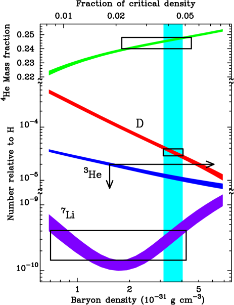
Figure 3: The relative abundance of light elements to Hidrogen. Note the large range of scales involved. From Ref. [10].

Nowadays, Big Bang nucleosynthesis (BBN) codes compute a chain of around 30 coupled nuclear reactions, to produce all the light elements up to beryllium-7.  Only the first four or five elements can be computed with accuracy better than 1% and compared with cosmological observations. These light elements are $H,{}^{4}\!He,D,{}^{3}\!He,{}^{7}\!Li$, and perhaps also ${}^{6}\!Li$. Their observed relative abundance to hydrogen is $[1:0.25:3\cdot 10^{-5}:2\cdot 10^{-5}:2\cdot 10^{-10}]$ with various errors, mainly systematic. The BBN codes calculate these abundances using the laboratory measured nuclear reaction rates, the decay rate of the neutron, the number of light neutrinos and the homogeneous FRW expansion of the universe, as a function of only one variable, the number density fraction of baryons to photons, $\eta\equiv n_{\rm B}/n_{\gamma}$. In fact, the present observations are only consistent, see Fig. 3 and Ref. [11, 10], with a very narrow range of values of

$$\eta_{10}\equiv 10^{10}\,\eta=4.6-5.9\,.$$ (45)

Such a small value of $\eta$ indicates that there is about one baryon per $10^{9}$ photons in the universe today. Any acceptable theory of baryogenesis should account for such a small number. Furthermore, the present baryon fraction of the critical density can be calculated from $\eta_{10}$ as [10]

$$\Omega_{\rm B}h^{2}=3.6271\times 10^{-3}\,\eta_{10}=0.0190\pm 0.0024\hskip 14.22636pt(95\%\ {\rm c.l.})$$ (46)

Clearly, this number is well below closure density, so baryons cannot account for all the matter in the universe, as I shall discuss below.

2.2.2 Neutrino decoupling

Just before the nucleosynthesis of the lightest elements in the early universe, weak interactions were too slow to keep neutrinos in thermal equilibrium with the plasma, so they decoupled. We can estimate the temperature at which decoupling occurred from the weak interaction cross section, $\sigma_{\rm w}\simeq G_{F}^{2}T^{2}$ at finite temperature $T$, where $G_{F}=1.2\times 10^{-5}$ GeV^-2 is the Fermi constant. The neutrino interaction rate, via W boson exchange in  $n+\nu\leftrightarrow p+e^{-}$ and  $p+\bar{\nu}\leftrightarrow n+e^{+}$, can be written as [8]

$$\Gamma_{\nu}=n_{\nu}\langle\sigma_{\rm w}|v|\rangle\simeq G_{F}^{2}T^{5}\,,$$ (47)

while the rate of expansion of the universe at that time ($g_{*}=10.75$) was $H\simeq 5.4\ T^{2}/M_{\rm P}$, where $M_{\rm P}=1.22\times 10^{19}$ GeV is the Planck mass. Neutrinos decouple when their interaction rate is slower than the universe expansion, $\Gamma_{\nu}\leq H$ or, equivalently, at $T_{\nu-{\rm dec}}\simeq 0.8$ MeV. Below this temperature, neutrinos are no longer in thermal equilibrium with the rest of the plasma, and their temperature continues to decay inversely proportional to the scale factor of the universe. Since neutrinos decoupled before $e^{+}e^{-}$ annihilation, the cosmic background of neutrinos has a temperature today lower than that of the microwave background of photons. Let us compute the difference. At temperatures above the the mass of the electron, $T>m_{e}=0.511$ MeV, and below 0.8 MeV, the only particle species contributing to the entropy of the universe are the photons ($g_{*}=2$) and the electron-positron pairs ($g_{*}=4\times{7\over 8}$); total number of degrees of freedom $g_{*}={11\over 2}$. At temperatures $T\simeq m_{e}$, electrons and positrons annihilate into photons, heating up the plasma (but not the neutrinos, which had decoupled already). At temperatures $T<m_{e}$, only photons contribute to the entropy of the universe, with $g_{*}=2$ degrees of freedom. Therefore, from the conservation of entropy, we find that the ratio of $T_{\gamma}$ and $T_{\nu}$ today must be

$${T_{\gamma}\over T_{\nu}}=\Big{(}{11\over 4}\Big{)}^{1/3}=1.401\hskip 14.22636pt\Rightarrow\hskip 14.22636ptT_{\nu}=1.945\ {\rm K}\,,$$ (48)

where I have used $T_{{}_{\rm CMB}}=2.725\pm 0.002$ K. We still have not measured such a relic background of neutrinos, and probably will remain undetected for a long time, since they have an average energy of order $10^{-4}$ eV, much below that required for detection by present experiments (of order GeV), precisely because of the relative weakness of the weak interactions. Nevertheless, it would be fascinating if, in the future, ingenious experiments were devised to detect such a background, since it would confirm one of the most robust features of Big Bang cosmology.

2.2.3 Matter-radiation equality

Relativistic species have energy densities proportional to the quartic power of temperature and therefore scale as $\rho_{\rm R}\propto a^{-4}$, while non-relativistic particles have essentially zero pressure and scale as $\rho_{\rm M}\propto a^{-3}$, see Eq. (38). Therefore, there will be a time in the evolution of the universe in which both energy densities are equal $\rho_{\rm R}(t_{\rm eq})=\rho_{\rm M}(t_{\rm eq})$. Since then both decay differently, and thus

$$1+z_{\rm eq}={a_{0}\over a_{\rm eq}}={\Omega_{\rm M}\over\Omega_{\rm R}}=3.1\times 10^{4}\ \Omega_{\rm M}h^{2}\,,$$ (49)

where I have used $\Omega_{\rm R}h^{2}=\Omega_{{}_{\rm CMB}}h^{2}+\Omega_{\nu}h^{2}=3.24\times 10^{-5}$ for three massless neutrinos at $T=T_{\nu}$. As I will show later, the matter content of the universe today is below critical, $\Omega_{\rm M}\simeq 0.3$, while $h\simeq 0.65$, and therefore $(1+z_{\rm eq})\simeq 3900$, or about $t_{\rm eq}=1.2\times 10^{3}\,(\Omega_{\rm M}h^{2})^{-2}\simeq 7\times 10^{4}$ years after the origin of the universe. Around the time of matter-radiation equality, the rate of expansion (18) can be written as ($a_{0}\equiv 1$)

$$H(a)=H_{0}\,\Big{(}\Omega_{\rm R}\,a^{-4}+\Omega_{\rm M}\,a^{-3}\Big{)}^{1/2}=H_{0}\,\Omega_{\rm M}^{1/2}\,a^{-3/2}\Big{(}1+{a_{\rm eq}\over a}\Big{)}^{1/2}\,.$$ (50)

The horizon size is the coordinate distance travelled by a photon since the beginning of the universe, $d_{H}\sim H^{-1}$, i.e. the size of causally connected regions in the universe. The comoving horizon size is then given by

$$d_{H}={c\over aH(a)}=c\,H_{0}^{-1}\Omega_{\rm M}^{-1/2}\,a^{1/2}\Big{(}1+{a_{\rm eq}\over a}\Big{)}^{-1/2}\,.$$ (51)

Thus the horizon size at matter-radiation equality ($a=a_{\rm eq}$) is

$$d_{H}(a_{\rm eq})={c\,H_{0}^{-1}\over\sqrt{2}}\,\Omega_{\rm M}^{-1/2}\,a_{\rm eq}^{1/2}\simeq 12\,(\Omega_{\rm M}h)^{-1}\,h^{-1}{\rm Mpc}\,.$$ (52)

This scale plays a very important role in theories of structure formation.

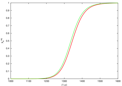
Figure 4: The equilibrium ionization fraction $X_{e}^{\rm eq}$ as a function of redshift. The two lines show the range of $\eta_{10}=4.6-5.9$.

2.2.4 Recombination and photon decoupling

As the temperature of the universe decreased, electrons could eventually become bound to protons to form neutral hydrogen. Nevertheless, there is always a non-zero probability that a rare energetic photon ionizes hydrogen and produces a free electron. The ionization fraction of electrons in equilibrium with the plasma at a given temperature is given by [8]

$${1-X_{e}^{\rm eq}\over X_{e}^{\rm eq}}={4\sqrt{2}\zeta(3)\over\sqrt{\pi}}\,\eta\,\left({T\over m_{e}}\right)^{3/2}\,e^{E_{\rm ion}/T}\,,$$ (53)

where $E_{\rm ion}=13.6$ eV is the ionization energy of hydrogen, and $\eta$ is the baryon-to-photon ratio (45). If we now use Eq. (44), we can compute the ionization fraction $X_{e}^{\rm eq}$ as a function of redshift $z$, see Fig. 4. Note that the huge number of photons with respect to electrons (in the ratio ${}^{4}\!He:H:\gamma\simeq 1:4:10^{10}$) implies that even at a very low temperature, the photon distribution will contain a sufficiently large number of high-energy photons to ionize a significant fraction of hydrogen. In fact, defining recombination as the time at which $X_{e}^{\rm eq}\equiv 0.1$, one finds that the recombination temperature is $T_{\rm rec}=0.3\ {\rm eV}\ll E_{\rm ion}$, for $\eta_{10}\simeq 5.2$. Comparing with the present temperature of the microwave background, we deduce the corresponding redshift at recombination, $(1+z_{\rm rec})\simeq 1270$.

Photons remain in thermal equilibrium with the plasma of baryons and electrons through elastic Thomson scattering, with cross section

$$\sigma_{{}_{T}}={8\pi\alpha^{2}\over 3m_{e}^{2}}=6.65\times 10^{-25}\ {\rm cm}^{2}=0.665\ {\rm barn}\,,$$ (54)

where $\alpha=1/137.036$  is the dimensionless electromagnetic coupling constant. The mean free path of photons $\lambda_{\gamma}$ in such a plasma can be estimated from the photon interaction rate, $\lambda_{\gamma}^{-1}\sim\Gamma_{\gamma}=n_{e}\sigma_{{}_{T}}$. For temperatures above a few eV, the mean free path is much smaller that the causal horizon at that time and photons suffer multiple scattering: the plasma is like a dense fog. Photons will decouple from the plasma when their interaction rate cannot keep up with the expansion of the universe and the mean free path becomes larger than the horizon size: the universe becomes transparent. We can estimate this moment by evaluating $\Gamma_{\gamma}=H$ at photon decoupling. Using $n_{e}=X_{e}\,\eta\,n_{\gamma}$, one can compute the decoupling temperature as $T_{\rm dec}=0.26$ eV, and the corresponding redshift as $(1+z_{\rm dec})\simeq 1100$. This redshift defines the so called last scattering surface, when photons last scattered off protons and electrons and travelled freely ever since. This decoupling occurred when the universe was approximately $t_{\rm dec}=1.8\times 10^{5}\,(\Omega_{\rm M}h^{2})^{-1/2}\simeq 5\times 10^{5}$ years old.

Figure 5: The Cosmic Microwave Background Spectrum seen by the FIRAS instrument on COBE. The left panel corresponds to the monopole spectrum, $T_{0}=2.725\pm 0.002$ K, where the error bars are smaller than the line width. The right panel shows the dipole spectrum, $\delta T_{1}=3.372\pm 0.014$ mK. From Ref. [12].

2.2.5 The microwave background

One of the most remarkable observations ever made my mankind is the detection of the relic background of photons from the Big Bang. This background was predicted by George Gamow and collaborators in the 1940s, based on the consistency of primordial nucleosynthesis with the observed helium abundance. They estimated a value of about 10 K, although a somewhat more detailed analysis by Alpher and Herman in 1950 predicted $T_{\gamma}\approx 5$ K. Unfortunately, they had doubts whether the radiation would have survived until the present, and this remarkable prediction slipped into obscurity, until Dicke, Peebles, Roll and Wilkinson [13] studied the problem again in 1965. Before they could measure the photon background, they learned that Penzias and Wilson had observed a weak isotropic background signal at a radio wavelength of 7.35 cm, corresponding to a blackbody temperature of $T_{\gamma}=3.5\pm 1$ K. They published their two papers back to back, with that of Dicke et al. explaining the fundamental significance of their measurement [6].

Since then many different experiments have confirmed the existence of the microwave background. The most outstanding one has been the Cosmic Background Explorer (COBE) satellite, whose FIRAS instrument measured the photon background with great accuracy over a wide range of frequencies ($\nu=1-97$ cm^-1), see Ref. [12], with a spectral resolution ${\Delta\nu\over\nu}=0.0035$. Nowadays, the photon spectrum is confirmed to be a blackbody spectrum with a temperature given by [12]

$$T_{{}_{\rm CMB}}=2.725\pm 0.002\ {\rm K}\ ({\rm systematic},\ 95\%\ {\rm c.l.})\ \pm 7\ \mu\!{\rm K}\ (1\sigma\ {\rm statistical})$$ (55)

In fact, this is the best blackbody spectrum ever measured, see Fig. 5, with spectral distortions below the level of 10 parts per million (ppm).

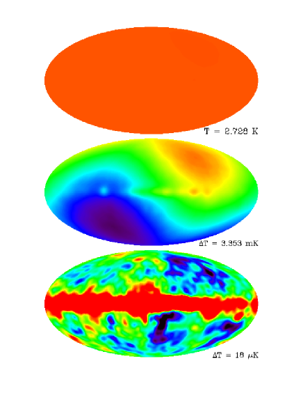
Figure 6: The Cosmic Microwave Background Spectrum seen by the DMR instrument on COBE. The top figure corresponds to the monopole, $T_{0}=2.725\pm 0.002$ K. The middle figure shows the dipole, $\delta T_{1}=3.372\pm 0.014$ mK, and the lower figure shows the quadrupole and higher multipoles, $\delta T_{2}=18\pm 2\ \mu$K. The central region corresponds to foreground by the galaxy. From Ref. [14].

Moreover, the differential microwave radiometer (DMR) instrument on COBE, with a resolution of about $7^{\circ}$ in the sky, has also confirmed that it is an extraordinarily isotropic background. The deviations from isotropy, i.e. differences in the temperature of the blackbody spectrum measured in different directions in the sky, are of the order of 20 $\mu$K on large scales, or one part in $10^{5}$, see Ref. [14]. There is, in fact, a dipole anisotropy of one part in $10^{3}$, $\delta T_{1}=3.372\pm 0.007$ mK (95% c.l.), in the direction of the Virgo cluster, $(l,b)=(264.14^{\circ}\pm 0.30,48.26^{\circ}\pm 0.30)$ (95% c.l.). Under the assumption that a Doppler effect is responsible for the entire CMB dipole, the velocity of the Sun with respect to the CMB rest frame is $v_{\odot}=371\pm 0.5$ km/s, see Ref. [12]. When subtracted, we are left with a whole spectrum of anisotropies in the higher multipoles (quadrupole, octupole, etc.), $\delta T_{2}=18\pm 2\ \mu$K (95% c.l.), see Ref. [14] and Fig. 6.

Soon after COBE, other groups quickly confirmed the detection of temperature anisotropies at around 30 $\mu$K and above, at higher multipole numbers or smaller angular scales. As I shall discuss below, these anisotropies play a crucial role in the understanding of the origin of structure in the universe.

2.3 Large-scale structure formation

Although the isotropic microwave background indicates that the universe in the past was extraordinarily homogeneous, we know that the universe today is not exactly homogeneous: we observe galaxies, clusters and superclusters on large scales. These structures are expected to arise from very small primordial inhomogeneities that grow in time via gravitational instability, and that may have originated from tiny ripples in the metric, as matter fell into their troughs. Those ripples must have left some trace as temperature anisotropies in the microwave background, and indeed such anisotropies were finally discovered by the COBE satellite in 1992. The reason why they took so long to be discovered was that they appear as perturbations in temperature of only one part in $10^{5}$.

While the predicted anisotropies have finally been seen in the CMB, not all kinds of matter and/or evolution of the universe can give rise to the structure we observe today. If we define the density contrast as [15]

$$\delta(\vec{x},a)\equiv{\rho(\vec{x},a)-\bar{\rho}(a)\over\bar{\rho}(a)}=\int d^{3}\vec{k}\ \delta_{k}(a)\ e^{i\vec{k}\cdot\vec{x}}\,,$$ (56)

where $\bar{\rho}(a)=\rho_{0}\,a^{-3}$ is the average cosmic density, we need a theory that will grow a density contrast with amplitude $\delta\sim 10^{-5}$ at the last scattering surface ($z=1100$) up to density contrasts of the order of $\delta\sim 10^{2}$ for galaxies at redshifts $z\ll 1$, i.e. today. This is a necessary requirement for any consistent theory of structure formation [16].

Furthermore, the anisotropies observed by the COBE satellite correspond to a small-amplitude scale-invariant primordial power spectrum of inhomogeneities

$$P(k)=\langle|\delta_{k}|^{2}\rangle\propto k^{n}\,,\hskip 14.22636pt{\rm with}\hskip 14.22636ptn=1\,,$$ (57)

where the brackets $\langle\cdot\rangle$ represent integration over an ensemble of different universe realizations. These inhomogeneities are like waves in the space-time metric. When matter fell in the troughs of those waves, it created density perturbations that collapsed gravitationally to form galaxies and clusters of galaxies, with a spectrum that is also scale invariant. Such a type of spectrum was proposed in the early 1970s by Edward R. Harrison, and independently by the Russian cosmologist Yakov B. Zel’dovich, see Ref. [17], to explain the distribution of galaxies and clusters of galaxies on very large scales in our observable universe.

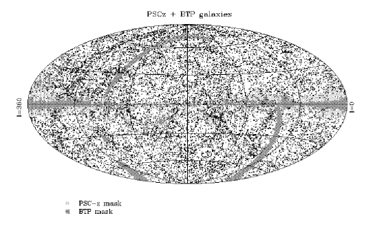
Figure 7: The IRAS Point Source Catalog redshift survey contains some 15,000 galaxies, covering over 83% of the sky up to redshifts of $z\leq 0.05$. We show here the projection of the galaxy distribution in galactic coordinates. From Ref. [18].

Today various telescopes – like the Hubble Space Telescope, the twin Keck telescopes in Hawaii and the European Southern Observatory telescopes in Chile – are exploring the most distant regions of the universe and discovering the first galaxies at large distances. The furthest galaxies observed so far are at redshifts of $z\simeq 5$, or 12 billion light years from the Earth, whose light was emitted when the universe had only about 5% of its present age. Only a few galaxies are known at those redshifts, but there are at present various catalogs like the CfA and APM galaxy catalogs, and more recently the IRAS Point Source redshift Catalog, see Fig. 7, and Las Campanas redshift surveys, that study the spatial distribution of hundreds of thousands of galaxies up to distances of a billion light years, or $z<0.1$, that recede from us at speeds of tens of thousands of kilometres per second. These catalogs are telling us about the evolution of clusters of galaxies in the universe, and already put constraints on the theory of structure formation. From these observations one can infer that most galaxies formed at redshifts of the order of $2-6$; clusters of galaxies formed at redshifts of order 1, and superclusters are forming now. That is, cosmic structure formed from the bottom up: from galaxies to clusters to superclusters, and not the other way around. This fundamental difference is an indication of the type of matter that gave rise to structure. The observed power spectrum of the galaxy matter distribution from a selection of deep redshift catalogs can be seen in Fig. 8.

We know from Big Bang nucleosynthesis that all the baryons in the universe cannot account for the observed amount of matter, so there must be some extra matter (dark since we don’t see it) to account for its gravitational pull. Whether it is relativistic (hot) or non-relativistic (cold) could be inferred from observations: relativistic particles tend to diffuse from one concentration of matter to another, thus transferring energy among them and preventing the growth of structure on small scales. This is excluded by observations, so we conclude that most of the matter responsible for structure formation must be cold. How much there is is a matter of debate at the moment. Some recent analyses suggest that there is not enough cold dark matter to reach the critical density required to make the universe flat. If we want to make sense of the present observations, we must conclude that some other form of energy permeates the universe. In order to resolve this issue, even deeper galaxy redshift catalogs are underway, looking at millions of galaxies, like the Sloan Digital Sky Survey (SDSS) and the Anglo-Australian two degree field (2dF) Galaxy Redshift Survey, which are at this moment taking data, up to redshifts of $z\mathrel{\mathop{\hbox{\lower 2.15277pt\hbox{$\sim$}\kern-8.00003pt\lower-3.01385pt\hbox{$<$}}}}0.5$, over a large region of the sky. These important observations will help astronomers determine the nature of the dark matter and test the validity of the models of structure formation.

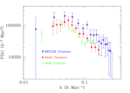
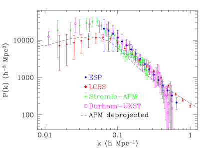
Figure 8: The left panel shows the matter power spectrum for clusters of galaxies, from three different cluster surveys. The right panel shows a compilation of the most recent estimates of the power spectrum of galaxy clustering, from four of the largest available redshift surveys of optically-selected galaxies, compared to the deprojected spectrum of the 2D APM galaxy survey. From Ref. [19].

Before COBE discovered the anisotropies of the microwave background there were serious doubts whether gravity alone could be responsible for the formation of the structure we observe in the universe today. It seemed that a new force was required to do the job. Fortunately, the anisotropies were found with the right amplitude for structure to be accounted for by gravitational collapse of primordial inhomogeneities under the attraction of a large component of non-relativistic dark matter. Nowadays, the standard theory of structure formation is a cold dark matter model with a non vanishing cosmological constant in a spatially flat universe. Gravitational collapse amplifies the density contrast initially through linear growth and later on via non-linear collapse. In the process, overdense regions decouple from the Hubble expansion to become bound systems, which start attracting eachother to form larger bound structures. In fact, the largest structures, superclusters, have not yet gone non-linear.

The primordial spectrum (57) is reprocessed by gravitational instability after the universe becomes matter dominated and inhomogeneities can grow. Linear perturbation theory shows that the growing mode  of small density contrasts go like [15, 16]

$$\delta(a)\propto a^{1+3\omega}=\left\{\begin{array}[]{ll}a^{2}\,,&\hskip 28.45274pta<a_{\rm eq}\\ a\,,&\hskip 28.45274pta>a_{\rm eq}\end{array}\right.$$ (58)

in the Einstein-de Sitter limit ($\omega=p/\rho=1/3$ and 0, for radiation and matter, respectively). There are slight deviations for $a\gg a_{\rm eq}$, if $\Omega_{\rm M}\neq 1$ or $\Omega_{\Lambda}\neq 0$, but we will not be concerned with them here. The important observation is that, since the density contrast at last scattering is of order $\delta\sim 10^{-5}$, and the scale factor has grown since then only a factor $z_{\rm dec}\sim 10^{3}$, one would expect a density contrast today of order $\delta_{0}\sim 10^{-2}$. Instead, we observe structures like galaxies, where $\delta\sim 10^{2}$. So how can this be possible? The microwave background shows anisotropies due to fluctuations in the baryonic matter component only (to which photons couple, electromagnetically). If there is an additional matter component that only couples through very weak interactions, fluctuations in that component could grow as soon as it decoupled from the plasma, well before photons decoupled from baryons. The reason why baryonic inhomogeneities cannot grow is because of photon pressure: as baryons collapse towards denser regions, radiation pressure eventually halts the contraction and sets up acoustic oscillations in the plasma that prevent the growth of perturbations, until photon decoupling. On the other hand, a weakly interacting cold dark matter component could start gravitational collapse much earlier, even before matter-radiation equality, and thus reach the density contrast amplitudes observed today. The resolution of this mismatch is one of the strongest arguments for the existence of a weakly interacting cold dark matter component of the universe.

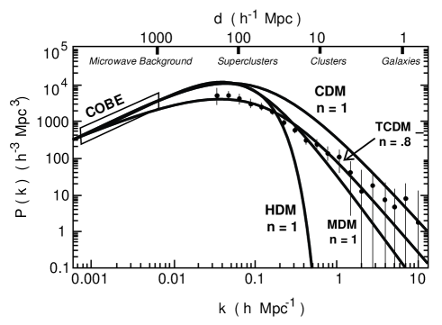
Figure 9: The power spectrum for cold dark matter (CDM), tilted cold dark matter (TCDM), hot dark matter (HDM), and mixed hot plus cold dark matter (MDM), normalized to COBE, for large-scale structure formation. From Ref. [20].

How much dark matter there is in the universe can be deduced from the actual power spectrum (the Fourier transform of the two-point correlation function of density perturbations) of the observed large scale structure. One can decompose the density contrast in Fourier components, see Eq. (56). This is very convenient since in linear perturbation theory individual Fourier components evolve independently. A comoving wavenumber $k$ is said to “enter the horizon” when $k=d_{H}^{-1}(a)=aH(a)$. If a certain perturbation, of wavelength $\lambda=k^{-1}<d_{H}(a_{\rm eq})$, enters the horizon before matter-radiation equality, the fast radiation-driven expansion prevents dark-matter perturbations from collapsing. Since light can only cross regions that are smaller than the horizon, the suppression of growth due to radiation is restricted to scales smaller than the horizon, while large-scale perturbations remain unaffected. This is the reason why the horizon size at equality, Eq. (52), sets an important scale for structure growth,

$$k_{\rm eq}=d_{H}^{-1}(a_{\rm eq})\simeq 0.083\,(\Omega_{\rm M}h)\,h\ {\rm Mpc}^{-1}\,.$$ (59)

The suppression factor can be easily computed from (58) as $f_{\rm sup}=(a_{\rm enter}/a_{\rm eq})^{2}=(k_{\rm eq}/k)^{2}$. In other words, the processed power spectrum $P(k)$ will have the form:

$$P(k)\propto\left\{\begin{array}[]{ll}k\,,&\hskip 28.45274ptk\ll k_{\rm eq}\\[5.69054pt] k^{-3}\,,&\hskip 28.45274ptk\gg k_{\rm eq}\end{array}\right.$$ (60)

This is precisely the shape that large-scale galaxy catalogs are bound to test in the near future, see Fig. 9. Furthermore, since relativistic Hot Dark Matter (HDM) transfer energy between clumps of matter, they will wipe out small scale perturbations, and this should be seen as a distinctive signature in the matter power spectra of future galaxy catalogs. On the other hand, non-relativistic Cold Dark Matter (CDM) allow structure to form on all scales via gravitational collapse. The dark matter will then pull in the baryons, which will later shine and thus allow us to see the galaxies.

Naturally, when baryons start to collapse onto dark matter potential wells, they will convert a large fraction of their potential energy into kinetic energy of protons and electrons, ionizing the medium. As a consequence, we expect to see a large fraction of those baryons constituting a hot ionized gas surrounding large clusters of galaxies. This is indeed what is observed, and confirms the general picture of structure formation.

3 DETERMINATION OF COSMOLOGICAL PARAMETERS

In this Section, I will restrict myself to those recent measurements of the cosmological parameters by means of standard cosmological techniques, together with a few instances of new results from recently applied techniques. We will see that a large host of observations are determining the cosmological parameters with some reliability of the order of 10%. However, the majority of these measurements are dominated by large systematic errors. Most of the recent work in observational cosmology has been the search for virtually systematic-free observables, like those obtained from the microwave background anisotropies, and discussed in Section 4.4. I will devote, however, this Section to the more ‘classical’ measurements of the following cosmological parameters: The rate of expansion $H_{0}$; the matter content $\Omega_{\rm M}$; the cosmological constant $\Omega_{\Lambda}$; the spatial curvature $\Omega_{K}$, and the age of the universe $t_{0}$.

These five basic cosmological parameters are not mutually independent. Using the homogeneity and isotropy on large scales observed by COBE, we can infer relationships between the different cosmological parameters through the Einstein-Friedmann equations. In particular, we can deduce the value of the spatial curvature from the Cosmic Sum Rule,

$$1=\Omega_{\rm M}+\Omega_{\Lambda}+\Omega_{K}\,,$$ (61)

or viceversa, if we determine that the universe is spatially flat from observations of the microwave background, we can be sure that the sum of the matter content plus the cosmological constant must be one.

Another relationship between parameters appears for the age of the universe. In a FRW cosmology, the cosmic expansion is determined by the Friedmann equation (8). Defining a new time and normalized scale factor,

$$y\equiv{a\over a_{0}}={1\over 1+z}\,,\hskip 56.9055pt\tau\equiv H_{0}(t-t_{0})\,,$$ (62)

we can write the Friedmann equation with the help of the Cosmic Sum Rule (19) as

$$y^{\prime}(\tau)=\Big{[}1+(y^{-1}-1)\Omega_{\rm M}+(y^{2}-1)\Omega_{\Lambda}\Big{]}^{1/2}\,,$$ (63)

with initial condition $y(0)=1,\ y^{\prime}(0)=1$. Therefore, the present age $t_{0}$ is a function of the other parameters, $t_{0}=f(H_{0},\Omega_{\rm M},\Omega_{\Lambda})$, determined from

$$t_{0}H_{0}=\int_{0}^{1}dy\,\Big{[}1+(y^{-1}-1)\Omega_{\rm M}+(y^{2}-1)\Omega_{\Lambda}\Big{]}^{-1/2}\,.$$ (64)

We show in Fig. 10 the contour lines for constant $t_{0}H_{0}$ in parameter space $(\Omega_{\rm M},\Omega_{\Lambda})$.

Figure 10: The contour lines correspond to equal  $t_{0}H_{0}=0.5-1.0,1.2,1.5,2.0$ and 5.0, from bottom to top, in parameter space $(\Omega_{\rm M},\Omega_{\Lambda})$. The line $t_{0}H_{0}=\infty$ would be indistinguishable from that of  $t_{0}H_{0}=5$. From Ref. [7].

There are two specific limits of interest: an open universe with $\Omega_{\Lambda}=0$, for which the age is given by

$$t_{0}H_{0}={1\over 1-\Omega_{\rm M}}-{\Omega_{\rm M}\over(1-\Omega_{\rm M})^{3/2}}\,\ln\left[{1+(1-\Omega_{\rm M})^{1/2}\over\Omega_{\rm M}^{1/2}}\right]=2\,\sum_{n=0}^{\infty}{(1-\Omega_{\rm M})^{n}\over(2n+1)(2n+3)}\,,$$ (65)

and a flat universe with $\Omega_{\Lambda}=1-\Omega_{\rm M}$, for which the age can also be expressed in compact form,

$$t_{0}H_{0}={2\over 3(1-\Omega_{\rm M})^{1/2}}\,\ln\left[{1+(1-\Omega_{\rm M})^{1/2}\over\Omega_{\rm M}^{1/2}}\right]={2\over 3}\,\sum_{n=0}^{\infty}{(1-\Omega_{\rm M})^{n}\over 2n+1}\,.$$ (66)

We have plotted these functions in Fig. 11. It is clear that in both cases $t_{0}H_{0}\to 2/3$ as $\Omega_{\rm M}\to 1$. We can now use these relations as a consistency check between the cosmological observations of $H_{0}$, $\Omega_{\rm M}$, $\Omega_{\Lambda}$ and $t_{0}$. Of course, we cannot measure the age of the universe directly, but only the age of its constituents: stars, galaxies, globular clusters, etc. Thus we can only find a lower bound on the age of the universe, $t_{0}\mathrel{\mathop{\hbox{\lower 2.15277pt\hbox{$\sim$}\kern-8.00003pt\lower-3.01385pt\hbox{$>$}}}}t_{\rm gal}+1.5$ Gyr. As we will see, this is not a trivial bound and, in several occasions, during the progress towards better determinations of the cosmological parameters, the universe seemed to be younger than its constituents, a logical inconsistency, of course, only due to an incorrect assessment of systematic errors [21].

Figure 11: The age of the universe as a function of the matter content, for an open and a flat universe. From Ref. [22].

In order to understand those recent measurements, one should also define what is known as the luminosity distance to an object in the universe. Imagine a source that is emitting light at a distance $d_{L}$ from a detector of area $dA$. The absolute luminosity ${\cal L}$ of such a source is nothing but the energy emitted per unit time. A standard candle is a luminous object that can be calibrated with some accuracy and therefore whose absolute luminosity is known, within certain errors. For example, Cepheid variable stars and type Ia supernovae are considered to be reasonable standard candles, i.e. their calibration errors are within bounds. The energy flux ${\cal F}$ received at the detector is the measured energy per unit time per unit area of the detector coming from that source. The luminosity distance $d_{L}$ is then defined as the radius of the sphere centered on the source for which the absolute luminosity would give the observed flux, $\ {\cal F}\equiv{\cal L}/4\pi d_{L}^{2}$. In a Friedmann-Robertson-Walker universe, light travels along null geodesics, $ds^{2}=0$, or, see Eq. (2),

$${dr\over\sqrt{1+a_{0}^{2}H_{0}^{2}\,r^{2}\,\Omega_{K}}}={1\over a_{0}^{2}H_{0}^{2}}\,{dz\over\sqrt{(1+z)^{2}(1+z\Omega_{\rm M})-z(2+z)\Omega_{\Lambda}}}\,,$$ (67)

which determines the coordinate distance $r=r(z,H_{0},\Omega_{\rm M},\Omega_{\Lambda})$, as a function of redshift $z$ and the other cosmological parameters. Now let us consider the effect of the universe expansion on the observed flux coming from a source at a certain redshift $z$ from us. First, the photon energy on its way here will be redshifted, and thus the observed energy $E_{0}=E/(1+z)$. Second, the rate of photon arrival will be time-delayed with respect to that emitted by the source, $dt_{0}=(1+z)dt$. Finally, the fraction of the area of the 2-sphere centered on the source that is covered by the detector is $dA/4\pi a_{0}^{2}\,r^{2}(z)$. Therefore, the total flux detected is

$${\cal F}={{\cal L}\over 4\pi a_{0}^{2}\,r^{2}(z)}\equiv{{\cal L}\over 4\pi d_{L}^{2}}\,.$$ (68)

The final expression for the luminosity distance $d_{L}$ as a function of redshift is thus given by [8]

$$H_{0}\,d_{L}=(1+z)\,|\Omega_{K}|^{-1/2}\,{\rm sinn}\left[|\Omega_{K}|^{1/2}\int_{0}^{z}{dz^{\prime}\over\sqrt{(1+z^{\prime})^{2}(1+z^{\prime}\Omega_{\rm M})-z^{\prime}(2+z^{\prime})\Omega_{\Lambda}}}\right]\,,$$ (69)

where ${\rm sinn}(x)=x\ {\rm if}\ K=0;\ \sin(x)\ {\rm if}\ K=+1\ {\rm and}\ \sinh(x)\ {\rm if}\ K=-1$. Expanding to second order around $z=0$, we obtain Eq. (6),

$$H_{0}\,d_{L}=z+{1\over 2}\Big{(}1-{\Omega_{\rm M}\over 2}+\Omega_{\Lambda}\Big{)}\,z^{2}+{\cal O}(z^{3})\,.$$ (70)

This expression goes beyond the leading linear term, corresponding to the Hubble law, into the second order term, which is sensitive to the cosmological parameters $\Omega_{\rm M}$ and $\Omega_{\Lambda}$. It is only recently that cosmological observations have gone far enough back into the early universe that we can begin to probe the second term, as I will discuss shortly. Higher order terms are not yet probed by cosmological observations, but they would contribute as important consistency checks.

Let us now pursue the analysis of the recent determinations of the most important cosmological parameters: the rate of expansion $H_{0}$, the matter content $\Omega_{\rm M}$, the cosmological constant $\Omega_{\Lambda}$, the spatial curvature $\Omega_{K}$, and the age of the universe $t_{0}$.

3.1 The rate of expansion $H_{0}$

Over most of last century the value of $H_{0}$ has been a constant source of disagreement [21]. Around 1929, Hubble measured the rate of expansion to be $H_{0}=500$ km s^-1Mpc^-1, which implied an age of the universe of order $t_{0}\sim 2$ Gyr, in clear conflict with geology. Hubble’s data was based on Cepheid standard candles that were incorrectly calibrated with those in the Large Magellanic Cloud. Later on, in 1954 Baade recalibrated the Cepheid distance and obtained a lower value, $H_{0}=250$ km s^-1Mpc^-1, still in conflict with ratios of certain unstable isotopes. Finally, in 1958 Sandage realized that the brightest stars in galaxies were ionized HII regions, and the Hubble rate dropped down to $H_{0}=60$ km s^-1 Mpc^-1, still with large (factor of two) systematic errors. Fortunately, in the past 15 years there has been significant progress towards the determination of $H_{0}$, with systematic errors approaching the 10% level. These improvements come from two directions. First, technological, through the replacement of photographic plates (almost exclusively the source of data from the 1920s to 1980s) with charged couple devices (CCDs), i.e. solid state detectors with excellent flux sensitivity per pixel, which were previously used successfully in particle physics detectors. Second, by the refinement of existing methods for measuring extragalactic distances (e.g. parallax, Cepheids, supernovae, etc.). Finally, with the development of completely new methods to determine $H_{0}$, which fall into totally independent and very broad categories: a) Gravitational lensing; b) Sunyaev-Zel’dovich effect; c) Extragalactic distance scale, mainly Cepheid variability and type Ia Supernovae; d) Microwave background anisotropies. I will review here the first three, and leave the last method for Section 4.4, since it involves knowledge about the primordial spectrum of inhomogeneities.

3.1.1 Gravitational lensing

Imagine a quasi-stellar object (QSO) at large redshift ($z\gg 1$) whose light is lensed by an intervening galaxy at redshift $z\sim 1$ and arrives to an observer at $z=0$. There will be at least two different images of the same background variable point source. The arrival times of photons from two different gravitationally lensed images of the quasar depend on the different path lengths and the gravitational potential traversed. Therefore, a measurement of the time delay and the angular separation of the different images of a variable quasar can be used to determine $H_{0}$ with great accuracy. This method, proposed in 1964 by Refsdael [23], offers tremendous potential because it can be applied at great distances and it is based on very solid physical principles [24].

Unfortunately, there are very few systems with both a favourable geometry (i.e. a known mass distribution of the intervening galaxy) and a variable background source with a measurable time delay. That is the reason why it has taken so much time since the original proposal for the first results to come out. Fortunately, there are now very powerful telescopes that can be used for these purposes. The best candidate to-date is the QSO $0957+561$, observed with the 10m Keck telescope, for which there is a model of the lensing mass distribution that is consistent with the measured velocity dispersion. Assuming a flat space with $\Omega_{\rm M}=0.25$, one can determine [25]

$$H_{0}=72\pm 7\ (1\sigma\ {\rm statistical})\ \pm 15\%\ ({\rm systematic})\ \ {\rm km\,s}^{-1}{\rm Mpc}^{-1}\,.$$ (71)

The main source of systematic error is the degeneracy between the mass distribution of the lens and the value of $H_{0}$. Knowledge of the velocity dispersion within the lens as a function of position helps constrain the mass distribution, but those measurements are very difficult and, in the case of lensing by a cluster of galaxies, the dark matter distribution in those systems is usually unknown, associated with a complicated cluster potential. Nevertheless, the method is just starting to give promising results and, in the near future, with the recent discovery of several systems with optimum properties, the prospects for measuring $H_{0}$ and lowering its uncertainty with this technique are excellent.

3.1.2 Sunyaev-Zel’dovich effect

As discussed in the previous Section, the gravitational collapse of baryons onto the potential wells generated by dark matter gave rise to the reionization of the plasma, generating an X-ray halo around rich clusters of galaxies, see Fig. 12. The inverse-Compton scattering of microwave background photons off the hot electrons in the X-ray gas results in a measurable distortion of the blackbody spectrum of the microwave background, known as the Sunyaev-Zel’dovich (SZ) effect. Since photons acquire extra energy from the X-ray electrons, we expect a shift towards higher frequencies of the spectrum, $(\Delta\nu/\nu)\simeq(k_{\rm B}T_{\rm gas}/m_{e}c^{2})\sim 10^{-2}$. This corresponds to a decrement of the microwave background temperature at low frequencies (Rayleigh-Jeans region) and an increment at high frequencies, see Ref. [26].

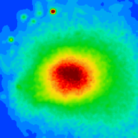
Figure 12: The Coma cluster of galaxies, seen here in an optical image (left) and an X-ray image (right), taken by the recently launched Chandra X-ray Observatory. From Ref. [27].

Measuring the spatial distribution of the SZ effect (3 K spectrum), together with a high resolution X-ray map ($10^{8}$ K spectrum) of the cluster, one can determine the density and temperature distribution of the hot gas. Since the X-ray flux is distance-dependent (${\cal F}={\cal L}/4\pi d_{L}^{2}$), while the SZ decrement is not (because the energy of the CMB photons increases as we go back in redshift, $\nu=\nu_{0}(1+z)$, and exactly compensates the redshift in energy of the photons that reach us), one can determine from there the distance to the cluster, and thus the Hubble rate $H_{0}$.

The advantages of this method are that it can be applied to large distances and it is based on clear physical principles. The main systematics come from possible clumpiness of the gas (which would reduce $H_{0}$), projection effects (if the clusters are prolate, $H_{0}$ could be larger), the assumption of hydrostatic equilibrium of the X-ray gas, details of models for the gas and electron densities, and possible contaminations from point sources. Present measurements give the value [26]

$$H_{0}=60\pm 10\ (1\sigma\ {\rm statistical})\ \pm 20\%\ ({\rm systematic})\ \ {\rm km\,s}^{-1}{\rm Mpc}^{-1}\,,$$ (72)

compatible with other determinations. A great advantage of this completely new and independent method is that nowadays more and more clusters are observed in the X-ray, and soon we will have high-resolution 2D maps of the SZ decrement from several balloon flights, as well as from future microwave background satellites, together with precise X-ray maps and spectra from the Chandra X-ray observatory recently launched by NASA, as well as from the European X-ray satellite XMM launched a few months ago by ESA, which will deliver orders of magnitude better resolution than the existing Einstein X-ray satellite.

3.1.3 Cepheid variability

Cepheids are low-mass variable stars with a period-luminosity relation based on the helium ionization cycles inside the star, as it contracts and expands. This time variability can be measured, and the star’s absolute luminosity determined from the calibrated relationship. From the observed flux one can then deduce the luminosity distance, see Eq. (69), and thus the Hubble rate $H_{0}$. The Hubble Space Telescope (HST) was launched by NASA in 1990 (and repaired in 1993) with the specific project of calibrating the extragalactic distance scale and thus determining the Hubble rate with 10% accuracy. The most recent results from HST are the following [28]

$$H_{0}=71\pm 4\ ({\rm random})\ \pm 7\ ({\rm systematic})\ \ {\rm km\,s}^{-1}{\rm Mpc}^{-1}\,.$$ (73)

The main source of systematic error is the distance to the Large Magellanic Cloud, which provides the fiducial comparison for Cepheids in more distant galaxies. Other systematic uncertainties that affect the value of $H_{0}$ are the internal extinction correction method used, a possible metallicity dependence of the Cepheid period-luminosity relation and cluster population incompleteness bias, for a set of 21 galaxies within 25 Mpc, and 23 clusters within $z\mathrel{\mathop{\hbox{\lower 2.15277pt\hbox{$\sim$}\kern-8.00003pt\lower-3.01385pt\hbox{$<$}}}}0.03$.

With better telescopes coming up soon, like the Very Large Telescope (VLT) interferometer of the European Southern Observatory (ESO) in the Chilean Atacama desert, with 4 synchronized telescopes by the year 2005, and the Next Generation Space Telescope (NGST) proposed by NASA for 2008, it is expected that much better resolution and therefore accuracy can be obtained for the determination of $H_{0}$.

3.2 The matter content $\Omega_{\rm M}$

In the 1920s Hubble realized that the so called nebulae were actually distant galaxies very similar to our own. Soon afterwards, in 1933, Zwicky found dynamical evidence that there is possibly ten to a hundred times more mass in the Coma cluster than contributed by the luminous matter in galaxies [29]. However, it was not until the 1970s that the existence of dark matter began to be taken more seriously. At that time there was evidence that rotation curves of galaxies did not fall off with radius and that the dynamical mass was increasing with scale from that of individual galaxies up to clusters of galaxies. Since then, new possible extra sources to the matter content of the universe have been accumulating:

$$\Omega_{\rm M} = \Omega_{\rm B,\ lum}\hskip 51.21504pt({\rm stars\ in\ galaxies})$$ (74)

$$+ \Omega_{\rm B,\ dark}\hskip 48.36958pt({\rm MACHOs?})$$ (75)

$$+ \Omega_{\rm CDM}\hskip 56.9055pt({\rm weakly\ interacting:\ axion,\ neutralino?})$$ (76)

$$+ \Omega_{\rm HDM}\hskip 56.9055pt({\rm massive\ neutrinos?})$$ (77)

The empirical route to the determination of $\Omega_{\rm M}$ is nowadays one of the most diversified of all cosmological parameters. The matter content of the universe can be deduced from the mass-to-light ratio of various objects in the universe; from the rotation curves of galaxies; from microlensing and the direct search of Massive Compact Halo Objects (MACHOs); from the cluster velocity dispersion with the use of the Virial theorem; from the baryon fraction in the X-ray gas of clusters; from weak gravitational lensing; from the observed matter distribution of the universe via its power spectrum; from the cluster abundance and its evolution; from direct detection of massive neutrinos at SuperKamiokande; from direct detection of Weakly Interacting Massive Particles (WIMPs) at DAMA and UKDMC, and finally from microwave background anisotropies. I will review here just a few of them.

3.2.1 Luminous matter

The most straight forward method of estimating $\Omega_{\rm M}$ is to measure the luminosity of stars in galaxies and then estimate the mass-to-light ratio, defined as the mass per luminosity density observed from an object, $\Upsilon={\cal M}/{\cal L}$. This ratio is usually expressed in solar units, ${\cal M}_{\odot}/{\cal L}_{\odot}$, so that for the sun $\Upsilon_{\odot}=1$. The luminosity of stars depends very sensitively on their mass and stage of evolution. The mass-to-light ratio of stars in the solar neighbourhood is of order $\Upsilon\approx 3$. For globular clusters and spiral galaxies we can determine their mass and luminosity independently and this gives $\Upsilon\approx$ few. For our galaxy,

$${\cal L}_{\rm gal}=(1.0\pm 0.3)\times 10^{8}\,h\,L_{\odot}\,{\rm Mpc}^{-3}\hskip 28.45274pt{\rm and}\hskip 28.45274pt\Upsilon_{\rm gal}=6\pm 3\,.$$ (78)

The contribution of galaxies to the luminosity density of the universe (in the visible-V spectral band, centered at $\sim 5500$ Å) is [30]

$${\cal L}_{V}=(1.7\pm 0.6)\times 10^{8}\,h\,L_{\odot}\,{\rm Mpc}^{-3}\,,$$ (79)

which can be translated into a mass density by multiplying by the observed $\Upsilon$ in that band,

$$\Omega_{\rm M}\,h=(6.1\pm 2.2)\times 10^{-4}\,\Upsilon_{V}\,.$$ (80)

All the luminous matter in the universe, from galaxies, clusters of galaxies, etc., account for $\Upsilon\approx 10$, and thus [31]

$$0.002\leq\Omega_{\rm lum}\,h\leq 0.006\,.$$ (81)

As a consequence, the luminous matter alone is far from the critical density. Moreover, comparing with the amount of baryons from Big Bang nucleosynthesis (46), we conclude that $\Omega_{\rm lum}\ll\Omega_{\rm B}$, so there must be a large fraction of baryons that are dark, perhaps in the form of very dim stars.

3.2.2 Rotation curves of spiral galaxies

The flat rotation curves of spiral galaxies provide the most direct evidence for the existence of large amounts of dark matter. Spiral galaxies consist of a central bulge and a very thin disk, stabilized against gravitational collapse by angular momentum conservation, and surrounded by an approximately spherical halo of dark matter. One can measure the orbital velocities of objects orbiting around the disk as a function of radius from the Doppler shifts of their spectral lines. The rotation curve of the Andromeda galaxy was first measured by Babcock in 1938, from the stars in the disk. Later it became possible to measure galactic rotation curves far out into the disk, and a trend was found [32]. The orbital velocity rose linearly from the center outward until it reached a typical value of 200 km/s, and then remained flat out to the largest measured radii. This was completely unexpected since the observed surface luminosity of the disk falls off exponentially with radius, $I(r)=I_{0}\exp(-r/r_{D})$, see Ref. [32]. Therefore, one would expect that most of the galactic mass is concentrated within a few disk lengths $r_{D}$, such that the rotation velocity is determined as in a Keplerian orbit, $v_{\rm rot}=(GM/r)^{1/2}\propto r^{-1/2}$. No such behaviour is observed. In fact, the most convincing observations come from radio emission (from the 21 cm line) of neutral hydrogen in the disk, which has been measured to much larger galactic radii than optical tracers. A typical case is that of the spiral galaxy NGC 6503, where $r_{D}=1.73$ kpc, while the furthest measured hydrogen line is at $r=22.22$ kpc, about 13 disk lengths away. The measured rotation curve is shown in Fig. 13 together with the relative components associated with the disk, the halo and the gas.

Figure 13: The rotation curve of the spiral galaxy NGC 6503, determined by radio observations of hydrogen gas in the disk [33]. The dashed line shows the rotation curve expected from the disk material alone, the dot-dashed line is from the dark matter halo alone.

Nowadays, thousands of galactic rotation curves are known, and all suggest the existence of about ten times more mass in the halos of spiral galaxies than in the stars of the disk. Recent numerical simulations of galaxy formation in a CDM cosmology [34] suggest that galaxies probably formed by the infall of material in an overdense region of the universe that had decoupled from the overall expansion. The dark matter is supposed to undergo violent relaxation and create a virialized system, i.e. in hydrostatic equilibrium. This picture has led to a simple model of dark-matter halos as isothermal spheres, with density profile $\rho(r)=\rho_{c}/(r_{c}^{2}+r^{2})$, where $r_{c}$ is a core radius and $\rho_{c}=v_{\infty}^{2}/4\pi G$, with $v_{\infty}$ equal to the plateau value of the flat rotation curve. This model is consistent with the universal rotation curve seen in Fig. 13. At large radii the dark matter distribution leads to a flat rotation curve. Adding up all the matter in galactic halos up to maximum radii, one finds $\Upsilon_{\rm halo}\geq 30\,h$, and therefore

$$\Omega_{\rm halo}\geq 0.03-0.05\,.$$ (82)

Of course, it would be extraordinary if we could confirm, through direct detection, the existence of dark matter in our own galaxy. For that purpose, one should measure its rotation curve, which is much more difficult because of obscuration by dust in the disk, as well as problems with the determination of reliable galactocentric distances for the tracers. Nevertheless, the rotation curve of the Milky Way has been measured and conforms to the usual picture, with a plateau value of the rotation velocity of 220 km/s, see Ref. [35]. For dark matter searches, the crucial quantity is the dark matter density in the solar neighbourhood, which turns out to be (within a factor of two uncertainty depending on the halo model) $\rho_{\rm DM}=0.3$ GeV/cm³. We will come back to direct searched of dark matter in a later subsection.

3.2.3 Microlensing

The existence of large amounts of dark matter in the universe, and in our own galaxy in particular, is now established beyond any reasonable doubt, but its nature remains a mystery. We have seen that baryons cannot account for the whole matter content of the universe; however, since the contribution of the halo (82) is comparable in magnitude to the baryon fraction of the universe (46), one may ask whether the galactic halo could be made of purely baryonic material in some non-luminous form, and if so, how one should search for it. In other words, are MACHOs the non-luminous baryons filling the gap between $\Omega_{\rm lum}$ and $\Omega_{\rm B}$? If not, what are they?

Let us start a systematic search for possibilities. They cannot be normal stars since they would be luminous; neither hot gas since it would shine; nor cold gas since it would absorb light and reemit in the infrared. Could they be burnt-out stellar remnants? This seems implausible since they would arise from a population of normal stars of which there is no trace in the halo. Neutron stars or black holes would typically arise from Supernova explosions and thus eject heavy elements into the galaxy, while the overproduction of helium in the halo is strongly constrained. They could be white dwarfs, i.e. stars not massive enough to reach supernova phase. Despite some recent arguments, a halo composed by white dwarfs is not rigorously excluded. Are they stars too small to shine? Perhaps M-dwarfs, stars with a mass $M\leq 0.1\,M_{\odot}$ which are intrinsically dim; however, very long exposure images of the Hubble Space Telescope restrict the possible M-dwarf contribution to the galaxy to be below 6%. The most plausible alternative is a halo composed of brown dwarfs with mass $M\leq 0.08\,M_{\odot}$, which never ignite hydrogen and thus shine only from the residual energy due to gravitational contraction. In fact, the extrapolation of the stellar mass function to small masses predicts a large number of brown dwarfs within normal stellar populations. A final possibility is primordial black holes (PBH), which could have been created in the early universe from early phase transitions [36], even before baryons were formed, and thus may be classified as non-baryonic. They could make a large contribution towards the total $\Omega_{\rm M}$, and still be compatible with Big Bang nucleosynthesis.

Figure 14: Geometry of the light deflection by a pointlike mass which gives two images of a source viewed by an observer. From Ref. [22].

Figure 15: The apparent lightcurve of a source if a pointlike MACHO passes through the line of sight with a transverse velocity $v$ and an impact parameter $b$. The amplification factor $A$ is shown in logarithmic scale to give the usual astronomical magnitude of an object. From Ref. [22].

Figure 16: The best candidate (LMC-1) for microlensing from the MACHO Collaboration in the direction of the Large Magellanic Cloud. A recent reanalysis of this event suggested an amplification factor  $A_{\rm max}=7.20\pm 0.09$, with achromaticity $A_{\rm red}/A_{\rm blue}=1.00\pm 0.05$, and a duration of  $\hat{t}=34.8\pm 0.2$. From Ref. [37].

Figure 17: Likelihood contours for MACHO mass $m$ (in units of solar mass) and halo fraction $f$ for a typical size halo. The plus sign shows the maximum likelihood estimate and the contours enclose regions of 68%, 90%, 95% and 99% probability. The panels are labeled according to different sets of selection criteria (A or B), and whether or not an LMC halo with MACHO fraction $f$ is included. From Ref. [38].

Whatever the arguments for or against baryonic objects as galactic dark matter, nothing would be more convincing than a direct detection of the various candidates, or their exclusion, in a direct search experiment. Fortunately, in 1986 Paczyński proposed a method for detecting faint stars in the halo of our galaxy [39]. The idea is based on the well known effect that a point-like mass deflector placed between an observer and a light source creates two different images, as shown in Fig. 14. When the source is exactly aligned with the deflector of mass $M_{D}$, the image would be an annulus, an Einstein ring, with radius

$$r_{\rm E}^{2}=4GM_{D}\,d\,,\hskip 28.45274pt{\rm where}\hskip 28.45274ptd={d_{1}d_{2}\over d_{1}+d_{2}}$$ (83)

is the reduced distance to the source, see Fig. 14. If the two images cannot be separated because their angular distance $\alpha$ is below the resolving power of the observer’s telescope, the only effect will be an apparent brightening of the star, an effect known as gravitational microlensing. The amplification factor is [39]

$$A={2+u^{2}\over u\sqrt{4+u^{2}}}\,,\hskip 28.45274pt{\rm where}\hskip 28.45274ptu\equiv{r\over r_{\rm E}}\,,$$ (84)

with $r$ the distance from the line of sight to the deflector. Imagine an observer on Earth watching a distant star in the Large Magellanic Cloud (LMC), 50 kpc away. If the galactic halo is filled with MACHOs, one of them will occasionally pass near the line of sight and thus cause the image of the background star to brighten. If the MACHO moves with velocity $v$ transverse to the line of sight, and if its impact parameter, i.e. the minimal distance to the line of sight, is $b$, then one expects an apparent lightcurve as shown in Fig. 15 for different values of $b/r_{\rm E}$. The natural time unit is $\Delta t=r_{\rm E}/v$, and the origin corresponds to the time of closest approach to the line of sight.

The probability for a target star to be lensed is independent of the mass of the dark matter object [39, 22]. For stars in the LMC one finds a probability, i.e. an optical depth for microlensing of the galactic halo, of approximately $\tau\sim 10^{-6}$. Thus, if one looks simultaneously at several millions of stars in the LMC during extended periods of time, one has a good chance of seeing at least a few of them brightened by a dark halo object. In order to be sure one has seen a microlensing event one has to monitor a large sample of stars long enough to identify the characteristic light curve shown in Fig. 15. The unequivocal signatures of such an event are the following: it must be a) unique (non-repetitive in time); b) time-symmetric; and c) achromatic (because of general covariance). These signatures allow one to discriminate against variable stars which constitute the background. The typical duration of the light curve is the time it takes a MACHO to cross an Einstein radius, $\Delta t=r_{\rm E}/v$. If the deflector mass is $1\ M_{\odot}$, the average microlensing time will be 3 months, for $10^{-2}\ M_{\odot}$ it is 9 days, for $10^{-4}\ M_{\odot}$ it is 1 day, and for $10^{-6}\ M_{\odot}$ it is 2 hours. A characteristic event, of duration 34 days, is shown in Fig. 16.

The first microlensing events towards the LMC were reported by the MACHO and EROS collaborations in 1993 [40, 41]. Nowadays, there are 12 candidates towards the LMC, 2 towards the SMC, around 40 towards the bulge of our own galaxy, and about 2 towards Andromeda, seen by AGAPE [42], with a slightly different technique based on pixel brightening rather than individual stars. Thus, microlensing is a well established technique with a rather robust future. In particular, it has allowed the MACHO and EROS collaboration to draw exclusion plots for various mass ranges in terms of their maximum allowed halo fraction, see Fig. 17. The MACHO Collaboration conclude in their 5-year analysis, see Ref. [38], that the spatial distribution of events is consistent with an extended lens distribution such as Milky Way or LMC halo, consisting partially of compact objects. A maximum likelihood analysis gives a MACHO halo fraction of 20% for a typical halo model with a 95% confidence interval of 8% to 50%. A 100% MACHO halo is ruled out at 95% c.l. for all except their most extreme halo model. The most likely MACHO mass is between 0.15 $M_{\odot}$ and 0.9 $M_{\odot}$, depending on the halo model. The lower mass is characteristic of white dwarfs, but a galactic halo composed primarily of white dwarfs is barely compatible with a range of observational constraints. On the other hand, if one wanted to attribute the observed events to brown dwarfs, one needs to appeal to a very non-standard density and/or velocity distribution of these objects. It is still unclear what sort of objects the microlensing experiments are seeing towards the LMC and where the lenses are. Nevertheless, the field is expanding, with several new experiments already underway, to search for clear signals of parallax, or binary systems, where the degeneracy between mass and distance can be resolved. For a discussion of those new results, see Ref. [37].

3.2.4 Virial theorem and large scale motion

Figure 18: The velocity and density fluctuation fields in the Supergalactic Plane as recovered by the POTENT method from the Mark III velocities of about 3,000 galaxies with 12 $h^{-1}$ smoothing. The vectors are projections of the 3D velocity field in the frame of the CMB. Coordinates are in units of 10 $h^{-1}$ Mpc. The marked structures are the Local Group (LG), the “Great Attractor” (GA), the Coma cluster “Great Wall” (GW), the Perseus-Pisces (PP) region and the “Southern Wall” (SW). From Ref. [43].

Clusters of galaxies are the largest gravitationally bound systems in the universe (superclusters are not yet in equilibrium). We know today several thousand clusters; they have typical radii of $1-5$ Mpc and typical masses of $2-9$ $\times 10^{14}\ M_{\odot}$. Zwicky noted in 1933 that these systems appear to have large amounts of dark matter [29]. He used the virial theorem (for a gravitationally bound system in equilibrium), $2\langle E_{\rm kin}\rangle=-\langle E_{\rm grav}\rangle$, where $\langle E_{\rm kin}\rangle={1\over 2}m\langle v^{2}\rangle$ is the average kinetic energy of one of the bound objects (galaxies) of mass $m$ and $\langle E_{\rm grav}\rangle=-m\langle GM/r\rangle$ is the average gravitational potential energy caused by the attraction of the other galaxies. Measuring the velocity dispersion $\langle v^{2}\rangle$ from the Doppler shifts of the spectral lines and estimating the geometrical size of the system gives an estimate of its total mass $M$. As Zwicky noted, this virial mass of clusters far exceeds their luminous mass, typically leading to a mass-to-light ratio $\Upsilon_{\rm cluster}=200\pm 70$. Assuming that the average cluster $\Upsilon$ is representative of the entire universe  one finds for the cosmic matter density [44]

$$\Omega_{\rm M}=0.24\pm 0.05\ (1\sigma\ {\rm statistical})\ \pm 0.09\ ({\rm systematic})\,.$$ (85)

On scales larger than clusters the motion of galaxies is dominated by the overall cosmic expansion. Nevertheless, galaxies exhibit peculiar velocities with respect to the global cosmic flow. For example, our Local Group of galaxies is moving with a speed of $627\pm 22$ km/s relative to the cosmic microwave background reference frame, towards the Great Attractor.

In the context of the standard gravitational instability theory of structure formation, the peculiar motions of galaxies are attributed to the action of gravity during the universe evolution, caused by the matter density inhomogeneities which give rise to the formation of structure. The observed large-scale velocity fields, together with the observed galaxy distributions, can then be translated into a measure for the mass-to-light ratio required to explain the large-scale flows. An example of the reconstruction of the matter density field in our cosmological vicinity from the observed velocity field is shown in Fig. 18. The cosmic matter density inferred from such analyses is [43, 45]

$$\Omega_{\rm M}>0.3\hskip 28.45274pt95\%\ {\rm c.l.}$$ (86)

Related methods that are more model-dependent give even larger estimates.

3.2.5 Baryon fraction in clusters

Since large clusters of galaxies form through gravitational collapse, they scoop up mass over a large volume of space, and therefore the ratio of baryons over the total matter in the cluster should be representative of the entire universe, at least within a 20% systematic error. Since the 1960s, when X-ray telescopes became available, it is known that galaxy clusters are the most powerful X-ray sources in the sky [46]. The emission extends over the whole cluster and reveals the existence of a hot plasma with temperature $T\sim 10^{7}-10^{8}$ K, where X-rays are produced by electron bremsstrahlung. Assuming the gas to be in hydrostatic equilibrium and applying the virial theorem one can estimate the total mass in the cluster, giving general agreement (within a factor of 2) with the virial mass estimates. From these estimates one can calculate the baryon fraction of clusters

$$f_{\rm B}h^{3/2}=0.03-0.08\hskip 28.45274pt\Rightarrow\hskip 28.45274pt{\Omega_{\rm B}\over\Omega_{\rm M}}\approx 0.15\,,\hskip 14.22636pt{\rm for}\hskip 8.53581pth=0.65\,,$$ (87)

which together with (81) indicates that clusters contain far more baryonic matter in the form of hot gas than in the form of stars in galaxies. Assuming this fraction to be representative of the entire universe, and using the Big Bang nucleosynthesis value of $\Omega_{\rm B}=0.05\pm 0.01$, for $h=0.65$, we find

$$\Omega_{\rm M}=0.3\pm 0.1\ ({\rm statistical})\ \pm 20\%\ ({\rm systematic})\,.$$ (88)

This value is consistent with previous determinations of $\Omega_{\rm M}$. If some baryons are ejected from the cluster during gravitational collapse, or some are actually bound in nonluminous objects like planets, then the actual value of $\Omega_{\rm M}$ is smaller than this estimate.

3.2.6 Weak gravitational lensing

Since the mid 1980s, deep surveys with powerful telescopes have observed huge arc-like features in galaxy clusters, see for instance Fig. 19. The spectroscopic analysis showed that the cluster and the giant arcs were at very different redshifts. The usual interpretation is that the arc is the image of a distant background galaxy which is in the same line of sight as the cluster so that it appears distorted and magnified by the gravitational lens effect: the giant arcs are essentially partial Einstein rings. From a systematic study of the cluster mass distribution one can reconstruct the shear field responsible for the gravitational distortion, see Ref. [47].

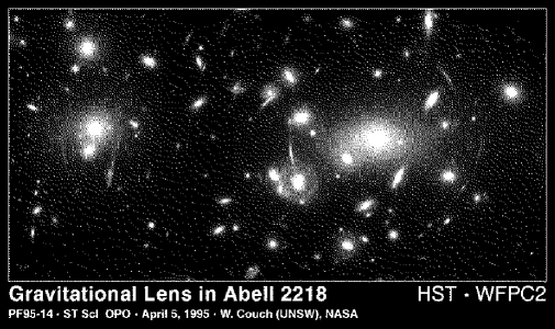
Figure 19: The most famous image of weak gravitational lensing around the Abell 2218 cluster, made by the Hubble Space Telescope. From Ref. [48].

This analysis shows that there are large amounts of dark matter in the clusters, in rough agreement with the virial mass estimates, although the lensing masses tend to be systematically larger. At present, the estimates indicate $\Omega_{\rm M}=0.2-0.3$ on scales $\mathrel{\mathop{\hbox{\lower 2.15277pt\hbox{$\sim$}\kern-8.00003pt\lower-3.01385pt\hbox{$<$}}}}6\,h^{-1}$ Mpc, while $\Omega_{\rm M}=0.4$ for the Corona Borealis supercluster, on scales of order 20 Mpc.

3.2.7 Structure formation and the matter power spectrum

One the most important constraints on the amount of matter in the universe comes from the present distribution of galaxies. As we mentioned in the Section 2.3, gravitational instability increases the primordial density contrast, seen at the last scattering surface as temperature anisotropies, into the present density field responsible for the large and the small scale structure.

Since the primordial spectrum is very approximately represented by a scale-invariant Gaussian random field, the best way to present the results of structure formation is by working with the 2-point correlation function in Fourier space (the equivalent to the Green’s function in QFT), the so-called power spectrum. If the reprocessed spectrum of inhomogeneities remains Gaussian, the power spectrum is all we need to describe the galaxy distribution. Non-Gaussian effects are expected to arise from the non-linear gravitational collapse of structure, and may be important at small scales [15].

The power spectrum measures the degree of inhomogeneity in the mass distribution on different scales. It depends upon a few basic ingredientes: a) the primordial spectrum of inhomogeneities, whether they are Gaussian or non-Gaussian, whether adiabatic (perturbations in the energy density) or isocurvature (perturbations in the entropy density), whether the primordial spectrum has tilt (deviations from scale-invariance), etc.; b) the recent creation of inhomogeneities, whether cosmic strings or some other topological defect from an early phase transition are responsible for the formation of structure today; and c) the cosmic evolution of the inhomogeneity, whether the universe has been dominated by cold or hot dark matter or by a cosmological constant since the beginning of structure formation, and also depending on the rate of expansion of the universe.

The working tools used for the comparison between the observed power spectrum and the predicted one are very precise N-body numerical simulations and theoretical models that predict the shape but not the amplitude of the present power spectrum. Even though a large amount of work has gone into those analyses, we still have large uncertainties about the nature and amount of matter necessary for structure formation. A model that has become a working paradigm is a flat cold dark matter model with a cosmological constant and $\Omega_{\rm M}=0.3-0.4$. This model will soon be confronted with very precise measurements from SDSS, 2dF, and several other large redshift catalogs, that are already taking data, see Section 4.5.

The observational constraints on the power spectrum have a huge lever arm of measurements at very different scales, mainly from the observed cluster abundance, on 10 Mpc scales, to the CMB fluctuations, on 1000 Mpc scales, which determines the normalization of the spectrum. At present, deep redshift surveys are probing scales between 100 and 1000 Mpc, which should begin to see the turnover corresponding to the peak of the power spectrum at $k_{\rm eq}$, see Figs. 8 and 9. The standard CDM model with $\Omega_{\rm M}=1$, normalized to the CMB fluctuations on large scales, is inconsistent with the cluster abundance. The power spectra of both a flat model with a cosmological constant or an open universe with $\Omega_{\rm M}=0.3$ (defined as $\Lambda$CDM and OCDM, respectively) can be normalized so that they agree with both the CMB and cluster observations. In the near future, galaxy survey observations will greatly improve the power spectrum constraints and will allow a measurement of $\Omega_{\rm M}$ from the shape of the spectrum. At present, these measurements suggest a low value of $\Omega_{\rm M}$, but with large uncertainties.

3.2.8 Cluster abundance and evolution

Rich clusters are the most recently formed gravitationally bound systems in the universe. Their number density as a function of time (or redshift) helps determine the amount of dark matter. The observed present ($z\sim 0$) cluster abundance provides a strong constraint on the normalization of the power spectrum of density perturbations on cluster scales. Both $\Lambda$CDM and OCDM are consistent with the observed cluster abundance at $z\sim 0$, see Fig. 20, while Standard CDM (Einstein-De Sitter model, with $\Omega_{\rm M}=1$), when normalized at COBE scales, produces too many clusters at all redshifts.

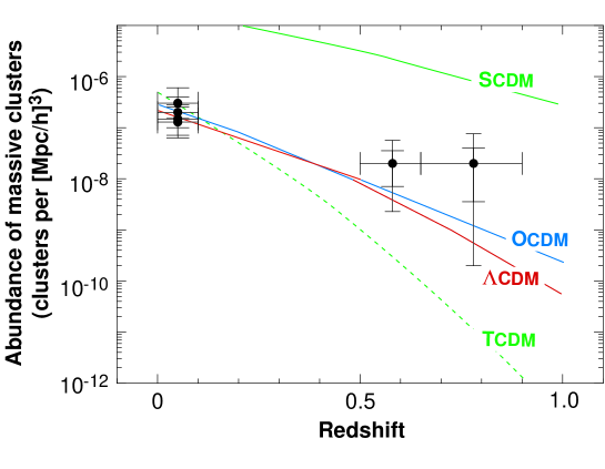
Figure 20: The evolution of the cluster abundance as a function of redshift, compared with observations from massive clusters. The four models are normalized to COBE. From Ref. [49].

The evolution of the cluster abundance with redshift breaks the degeneracy among the models at $z\sim 0$. The low-mass models (Open and $\Lambda$-CDM) predict a relatively small change in the number density of rich clusters as a function of redshift because, due to the low density, hardly any structure growth occurs since $z\sim 1$. The high-mass models (Tilted and Standard CDM) predict that structure has grown steadily and rich clusters only formed recently: the number density of rich clusters at $z\sim 1$ is predicted to be exponentially smaller than today. The observation of a single massive cluster is enough to rule out the $\Omega_{\rm M}=1$ model. In fact, three clusters have been seen, suggesting a low density universe [50],

$$\Omega_{\rm M}=0.25^{\ \ +0.15}_{\ \ -0.10}\ (1\sigma\ {\rm statistical})\ \pm 20\%\ ({\rm systematic})\,.$$ (89)

But one should be cautious. There is the caveat that for this constraint it is assumed that the initial spectrum of density perturbations is Gaussian, as predicted in the simplest models of inflation, but that has not yet been confirmed observationally on cluster scales.

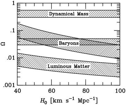
Figure 21: The observed cosmic matter components as functions of the Hubble expansion parameter. The luminous matter component is given by Eq. (81); the galactic halo component is the horizontal band, Eq. (82), crossing the baryonic component from BBN, Eq. (46); and the dynamical mass component from large scale structure analysis is given by Eq. (88). Note that in the range $H_{0}=70\pm 7$ km/s/Mpc, there are three dark matter problems, see the text.

3.2.9 Summary of the matter content

We can summarize the present situation with Fig. 21, for $\Omega_{\rm M}$ as a function of $H_{0}$. There are four bands, the luminous matter $\Omega_{\rm lum}$; the baryon content $\Omega_{\rm B}$, from BBN; the galactic halo component $\Omega_{\rm halo}$, and the dynamical mass from clusters, $\Omega_{\rm M}$. From this figure it is clear that there are in fact three dark matter problems: The first one is where are 90% of the baryons. Between the fraction predicted by BBN and that seen in stars and diffuse gas there is a huge fraction which is in the form of dark baryons. They could be in small clumps of hydrogen that have not started thermonuclear reactions and perhaps constitute the dark matter of spiral galaxies’ halos. Note that although $\Omega_{\rm B}$ and $\Omega_{\rm halo}$ coincide at $H_{0}\simeq 70$ km/s/Mpc, this could be just a coincidence. The second problem is what constitutes 90% of matter, from BBN baryons to the mass inferred from cluster dynamics. This is the standard dark matter problem and could be solved by direct detection of a weakly interacting massive particle in the laboratory. And finally, since we know from observations of the CMB, see Section 4.4, that the universe is flat, what constitutes around 60% of the energy density, from dynamical mass to critical density, $\Omega_{0}=1$? One possibility could be that the universe is dominated by a diffuse vacuum energy, i.e. a cosmological constant, which only affects the very large scales. Alternatively, the theory of gravity (general relativity) may need to be modified on large scales, e.g. due to quantum gravity effects. The need to introduce an effective cosmological constant on large scales is nowadays the only reason why gravity may need to be modified at the quantum level. Since we still do not have a quantum theory of gravity, such a proposal is still very speculative, and most of the approaches simply consider the inclusion of a cosmological constant as a phenomenological parameter.

3.2.10 Massive neutrinos

One of the ‘usual suspects’ when addressing the problem of dark matter are neutrinos. They are the only candidates known to exist. If neutrinos have a mass, could they constitute the missing matter? We know from the Big Bang theory, see Section 2.2.2, that there is a cosmic neutrino background at a temperature of approximately 2K. This allows one to compute the present number density in the form of neutrinos, which turns out to be, for massless neutrinos, $n_{\nu}(T_{\nu})={3\over 11}\,n_{\gamma}(T_{\gamma})=112\ {\rm cm}^{-3}$, per species of neutrino. If neutrinos have mass, as recent experiments seem to suggest, see Fig. 22, the cosmic energy density in massive neutrinos would be $\rho_{\nu}=\sum n_{\nu}m_{\nu}={3\over 11}\,n_{\gamma}\,\sum m_{\nu}$, and therefore its contribution today,

$$\Omega_{\nu}h^{2}={\sum m_{\nu}\over 94\ {\rm eV}}\,.$$ (90)

The discussion in the previous Sections suggest that $\Omega_{\rm M}\leq 0.4$, and thus, for any of the three families of neutrinos, $m_{\nu}\leq 40$ eV. Note that this limit improves by six orders of magnitude the present bound on the tau-neutrino mass [51]. Supposing that the missing mass in non-baryonic cold dark matter arises from a single particle dark matter (PDM) component, its contribution to the critical density is bounded by  $0.05\leq\Omega_{\rm PDM}h^{2}\leq 0.4$, see Fig. 21.

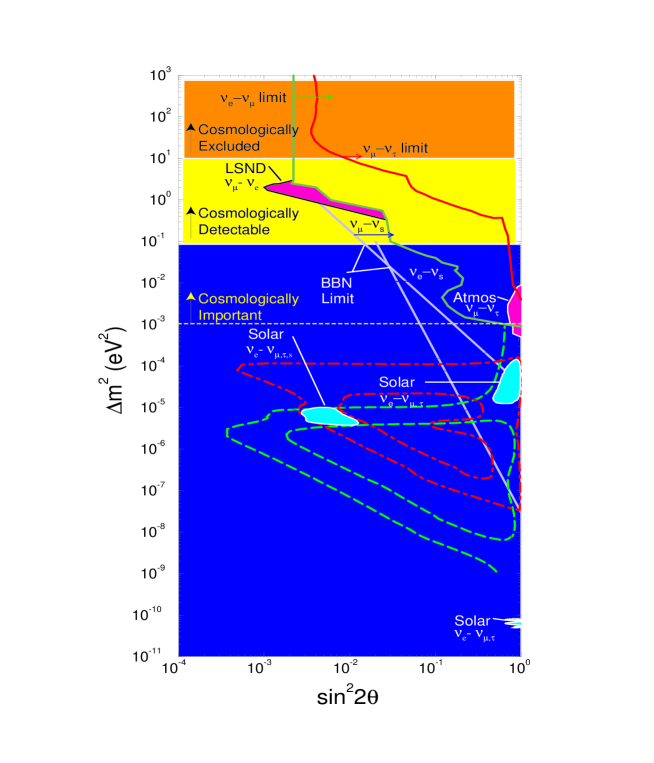
Figure 22: The neutrino parameter space, mixing angle against $\Delta m^{2}$, including the results from the different solar and atmospheric neutrino oscillation experiments. Note the threshold of cosmologically important masses, cosmologically detectable neutrinos (by CMB and LSS observations), and cosmologically excluded range of masses. From Ref. [52].

I will now go through the various logical arguments that exclude neutrinos as the dominant component of the missing dark matter in the universe. Is it possible that neutrinos with a mass  $4\ {\rm eV}\leq m_{\nu}\leq 40$ eV be the non-baryonic PDM component? For instance, could massive neutrinos constitute the dark matter halos of galaxies? For neutrinos to be gravitationally bound to galaxies it is necessary that their velocity be less that the escape velocity $v_{\rm esc}$, and thus their maximum momentum is $p_{\rm max}=m_{\nu}\,v_{\rm esc}$. How many neutrinos can be packed in the halo of a galaxy? Due to the Pauli exclusion principle, the maximum number density is given by that of a completely degenerate Fermi gas with momentum $p_{\rm F}=p_{\rm max}$, i.e. $n_{\rm max}=p_{\rm max}^{3}/3\pi^{2}$. Therefore, the maximum local density in dark matter neutrinos is $\rho_{\rm max}=n_{\rm max}m_{\nu}=m_{\nu}^{4}\,v_{\rm esc}^{3}/3\pi^{2}$, which must be greater than the typical halo density $\rho_{\rm halo}=0.3$ GeV cm^-3. For a typical spiral galaxy, this constraint, known as the Tremaine-Gunn limit, gives $m_{\nu}\geq 40$ eV, see Ref. [53]. However, this mass, even for a single species, say the tau-neutrino, gives a value for $\Omega_{\nu}h^{2}=0.5$, which is far too high for structure formation. Neutrinos of such a low mass would constitute a relativistic hot dark matter component, which would wash-out structure below the supercluster scale, against evidence from present observations, see Fig. 22. Furthermore, applying the same phase-space argument to the neutrinos as dark matter in the halo of dwarf galaxies gives $m_{\nu}\geq 100$ eV, beyond closure density (90). We must conclude that the simple idea that light neutrinos could constitute the particle dark matter on all scales is ruled out. They could, however, still play a role as a sub-dominant hot dark matter component in a flat CDM model. In that case, a neutrino mass of order 1 eV is not cosmological excluded, see Fig. 22.

Another possibility is that neutrinos have a large mass, of order a few GeV. In that case, their number density at decoupling, see Section 2.2.2, is suppressed by a Boltzmann factor, $\sim\exp(-m_{\nu}/T_{\rm dec})$. For masses $m_{\nu}>T_{\rm dec}\simeq 0.8$ MeV, the present energy density has to be computed as a solution of the corresponding Boltzmann equation. Apart from a logarithmic correction, one finds $\Omega_{\nu}h^{2}\simeq 0.1(10\ {\rm GeV}/m_{\nu})^{2}$ for Majorana neutrinos and slightly smaller for Dirac neutrinos. In either case, neutrinos could be the dark matter only if their mass was a few GeV. Laboratory limits for $\nu_{\tau}$ of around 18 MeV [51], and much more stringent ones for $\nu_{\mu}$ and $\nu_{e}$, exclude the known light neutrinos. However, there is always the possibility of a fourth unknown heavy and stable (perhaps sterile) neutrino. If it couples to the Z boson and has a mass below 45 GeV for Dirac neutrinos (39.5 GeV for Majorana neutrinos), then it is ruled out by measurements at LEP of the invisible width of the Z. There are two logical alternatives, either it is a sterile neutrino (it does not couple to the Z), or it does couple but has a larger mass. In the case of a Majorana neutrino (its own antiparticle), their abundance, for this mass range, is too small for being cosmologically relevant, $\Omega_{\nu}h^{2}\leq 0.005$. If it were a Dirac neutrino there could be a lepton asymmetry, which may provide a higher abundance (similar to the case of baryogenesis). However, neutrinos scatter on nucleons via the weak axial-vector current (spin-dependent) interaction. For the small momentum transfers imparted by galactic WIMPs, such collisions are essentially coherent over an entire nucleus, leading to an enhancement of the effective cross section. The relatively large detection rate in this case allowes one to exclude fourth-generation Dirac neutrinos for the galactic dark matter [54]. Anyway, it would be very implausible to have such a massive neutrino today, since it would have to be stable, with a life-time greater than the age of the universe, and there is no theoretical reason to expect a massive sterile neutrino that does not oscillate into the other neutrinos.

Of course, the definitive test to the possible contribution of neutrinos to the overall density of the universe would be to measure directly their mass in laboratory experiments. There are at present two types of experiments: neutrino oscillation experiments, which measure only differences in squared masses, and direct mass-searches experiments, like the tritium $\beta$-spectrum and the neutrinoless double-$\beta$ decay experiments, which measure directly the mass of the electron neutrino and give a bound $m_{\nu_{e}}\mathrel{\mathop{\hbox{\lower 2.15277pt\hbox{$\sim$}\kern-8.00003pt\lower-3.01385pt\hbox{$<$}}}}$ 2 eV. Neutrinos with such a mass could very well constitute the HDM component of the universe, $\Omega_{\rm HDM}\mathrel{\mathop{\hbox{\lower 2.15277pt\hbox{$\sim$}\kern-8.00003pt\lower-3.01385pt\hbox{$<$}}}}0.15$. The oscillation experiments give a variety of possibilities for $\Delta\,m_{\nu}^{2}=0.3-3\ {\rm eV}^{2}$ from LSND (not yet confirmed), to the atmospheric neutrino oscillations from SuperKamiokande ($\Delta\,m_{\nu}^{2}\simeq 3\times 10^{-3}\ {\rm eV}^{2}$) and the solar neutrino oscillations ($\Delta\,m_{\nu}^{2}\simeq 10^{-5}\ {\rm eV}^{2}$). Only the first two possibilities would be cosmologically relevant, see Fig. 22.

3.2.11 Weakly Interacting Massive Particles

Unless we drastically change the theory of gravity on large scales, baryons cannot make up the bulk of the dark matter. Massive neutrinos are the only alternative among the known particles, but they are essentially ruled out as a universal dark matter candidate, even if they may play a subdominant role as a hot dark matter component. There remains the mystery of what is the physical nature of the dominant cold dark matter component.

Something like a heavy stable neutrino, a generic Weakly Interacting Massive Particle (WIMP), could be a reasonable candidate because its present abundance could fall within the expected range,

$$\Omega_{\rm PDM}h^{2}\sim{G^{3/2}T_{0}^{3}h^{2}\over H_{0}^{2}\langle\sigma_{\rm ann}v_{\rm rel}\rangle}={3\times 10^{-27}\ {\rm cm}^{3}{\rm s}^{-1}\over\langle\sigma_{\rm ann}v_{\rm rel}\rangle}\,.$$ (91)

Here $v_{\rm rel}$ is the relative velocity of the two incoming dark matter particles and the brackets $\langle\dots\rangle$ denote a thermal average at the freeze-out temperature, $T_{\rm f}\simeq m_{\rm PDM}/20$, when the dark matter particles go out of equilibrium with radiation. The value of $\langle\sigma_{\rm ann}v_{\rm rel}\rangle$ needed for $\Omega_{\rm PDM}\approx 1$ is remarkably close to what one would expect for a WIMP with a mass $m_{\rm PDM}=100$ GeV,  $\langle\sigma_{\rm ann}v_{\rm rel}\rangle\sim\alpha^{2}/8\pi\,m_{\rm PDM}\sim 3\times 10^{-27}\ {\rm cm}^{3}{\rm s}^{-1}$. We still do not know whether this is just a coincidence or an important hint on the nature of dark matter.

Figure 23: The maximum likelihood region from the annual-modulation signal consistent with a neutralino of mass $\ m_{\chi}=59^{\ +17}_{\ -14}$ GeV and a proton cross section of $\ \xi\sigma_{p}=7.0^{\ +0.4}_{\ -1.2}\times 10^{-6}$ pb, see the text. The scatter plot represents the theoretical predictions of a generic MSSM. From Ref. [56].

There are a few theoretical candidates for WIMPs, like the neutralino, coming from supersymmetric extensions of the standard model of particle physics, but at present there is no empirical evidence that such extensions are indeed realized in nature. In fact, the non-observation of supersymmetric particles at current accelerators places stringent limits on the neutralino mass and interaction cross section [57].

If WIMPs constitute the dominant component of the halo of our galaxy, it is expected that some may cross the Earth at a reasonable rate to be detected. The direct experimental search for them rely on elastic WIMP collisions with the nuclei of a suitable target. Dark matter WIMPs move at a typical galactic virial velocity of around $200-300$ km/s, depending on the model. If their mass is in the range $10-100$ GeV, the recoil energy of the nuclei in the elastic collision would be of order 10 keV. Therefore, one should be able to identify such energy depositions in a macroscopic sample of the target. There are at present three different methods: First, one could search for scintillation light in NaI crystals or in liquid xenon; second, search for an ionization signal in a semiconductor, typically a very pure germanium crystal; and third, use a cryogenic detector at 10 mK and search for a measurable temperature increase of the sample. The main problem with such a type of experiment is the low expected signal rate, with a typical number below 1 event/kg/day. To reduce natural radioactive contamination one must use extremely pure substances, and to reduce the background caused by cosmic rays requires that these experiments be located deeply underground.

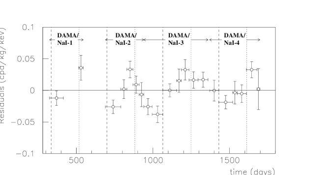
Figure 24: The DAMA experiment sees an annual variation, of order 7%, in the WIMP flux due to the Earth’s motion around the Sun. The model independent residual rate in the lowest ($2-6$ keV) cumulative energy interval (in counts per day/kg/keV) is shown as a function of time since 1 January of the first year of data taking. The expected behaviour of a WIMP signal is a cosine function with a minimum (maximum) roughly at the dashed (dotted) vertical lines. From Ref. [56].

The best limits on WIMP scattering cross sections come from some germanium experiments [58], as well as from the NaI scintillation detectors of the UK dark matter collaboration (UKDMC) in the Boulby salt mine in England [59], and the DAMA experiment in the Gran Sasso laboratory in Italy [56]. Current experiments already touch the parameter space expected from supersymmetric particles, see Fig. 23, and therefore there is a chance that they actually discover the nature of the missing dark matter. The problem, of course, is to attribute a tentative signal unambiguously to galactic WIMPs rather than to some unidentified radioactive background.

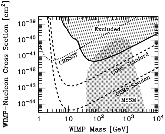
Figure 25: Exclusion range for the spin-independent WIMP scattering cross section per nucleon from the NaI experiments and the Ge detectors. Also shown is the range of expected counting rates for neutralinos in the MSSM. The search goals for the upcoming large-scale cryogenic detectors CRESST and CDMS are also shown. From Ref. [22].

One specific signature is the annual modulation which arises as the Earth moves around the Sun. Therefore, the net speed of the Earth relative to the galactic dark matter halo varies, causing a modulation of the expected counting rate. The DAMA/NaI experiment has actually reported such a modulation signal, see Fig. 24, from the combined analysis of their 4-year data [56], which provides a confidence level of 99.6% for a neutralino mass of $\ m_{\chi}=52^{\ +10}_{\ -8}$ GeV and a proton cross section of $\ \xi\sigma_{p}=7.2^{\ +0.4}_{\ -0.9}\times 10^{-6}$ pb, where $\xi=\rho_{\chi}/0.3$ GeV cm^-3 is the local neutralino energy density in units of the galactic halo density. There has been no confirmation yet of this result from other dark matter search groups, but hopefully in the near future we will have much better sensitivity at low masses from the Cryogenic Rare Event Search with Superconducting Thermometers (CRESST) experiment at Gran Sasso as well as at weaker cross sections from the CDMS experiment at Stanford and the Soudan mine, see Fig. 25. The CRESST experiment [60] uses sapphire crystals as targets and a new method to simultaneously measure the phonons and the scintillating light from particle interactions inside the crystal, which allows excellent background discrimination. Very recently there has been the interesting proposal of a completely new method based on a Superheated Droplet Detector (SDD), which claims to have already a similar sensitivity as the more standard methods described above, see Ref. [61].

There exist other indirect methods to search for galactic WIMPs [62]. Such particles could self-annihilate at a certain rate in the galactic halo, producing a potentially detectable background of high energy photons or antiprotons. The absence of such a background in both gamma ray satellites and the Alpha Matter Spectrometer [63] imposes bounds on their density in the halo. Alternatively, WIMPs traversing the solar system may interact with the matter that makes up the Earth or the Sun so that a small fraction of them will lose energy and be trapped in their cores, building up over the age of the universe. Their annihilation in the core would thus produce high energy neutrinos from the center of the Earth or from the Sun which are detectable by neutrino telescopes. In fact, SuperKamiokande already covers a large part of SUSY parameter space. In other words, neutrino telescopes are already competitive with direct search experiments. In particular, the AMANDA experiment at the South Pole [64], which is expected to have $10^{3}$ Cherenkov detectors 2.3 km deep in very clear ice, over a volume $\sim 1$ km³, is competitive with the best direct searches proposed. The advantages of AMANDA are also directional, since the arrays of Cherenkov detectors will allow one to reconstruct the neutrino trajectory and thus its source, whether it comes from the Earth or the Sun.

3.3 The cosmological constant $\Omega_{\Lambda}$

A cosmological constant is a term in the Einstein equations, see Eq. (1), that corresponds to the energy density of the vacuum of quantum field theories, $\Lambda\equiv 8\pi G\rho_{v}$, see Ref. [65]. These theories predict a value of order $\rho_{v}\sim M_{\rm P}^{4}\simeq 5\times 10^{93}$ g/cm³, which is about 123 orders of magnitude larger than the critical density (14). Such a discrepancy is one of the biggest problems of theoretical physics [66]. It has always been assumed that quantum gravity effects, via some as yet unknown symmetry, would exactly cancel the cosmological constant, but this remains a downright speculation. Moreover, one of the difficulties with a non-zero value for $\Lambda$ is that it appears coincidental that we are now living at a special epoch when the cosmological constant starts to dominate the dynamics of the universe, and that it will do so forever after, see Section 2.1.2 and Eq. (22). Nevertheless, ever since Einstein introduced it in 1917, this ethereal constant has been invoked several times in history to explain a number of apparent crises, always to disappear under further scrutiny [21].

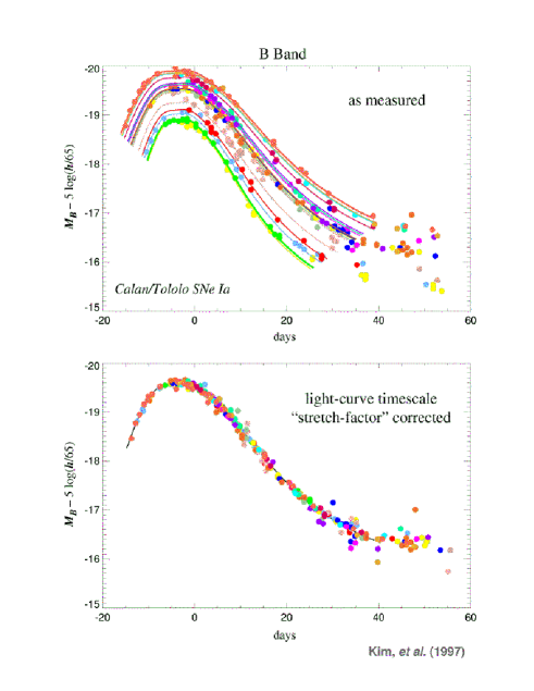
Figure 26: The Type Ia supernovae observed nearby show a relationship between their absolute luminosity and the timescale of their light curve: the brighter supernovae are slower and the fainter ones are faster. A simple linear relation between the absolute magnitude and a “stretch factor” multiplying the light curve timescale fits the data quite well. From Ref. [68].

In spite of the theoretical prejudice towards $\Lambda=0$, there are new observational arguments for a non-zero value. The most compelling ones are recent evidence that we live in a flat universe, from observations of CMB anisotropies, together with strong indications of a low mass density universe ($\Omega_{\rm M}<1$), from the large scale distribution of galaxies, clusters and voids, that indicate that some kind of dark energy must make up the rest of the energy density up to critical, i.e. $\Omega_{\Lambda}=1-\Omega_{\rm M}$. In addition, the discrepancy between the ages of globular clusters and the expansion age of the universe may be cleanly resolved with $\Lambda\neq 0$. Finally, there is growing evidence for an accelerating universe from observations of distant supernovae. I will now discuss the different arguments one by one.

The only known way to reconcile a low mass density with a flat universe is if an additional “dark” energy dominates the universe today. It would have to resist gravitational collapse, otherwise it would have been detected already as part of the energy in the halos of galaxies. However, if most of the energy of the universe resists gravitational collapse, it is impossible for structure in the universe to grow. This dilemma can be resolved if the hypothetical dark energy was negligible in the past and only recently became the dominant component. According to general relativity, this requires that the dark energy have negative pressure, since the ratio of dark energy to matter density goes like $a(t)^{-3p/\rho}$. This argument [67] would rule out almost all of the usual suspects, such as cold dark matter, neutrinos, radiation, and kinetic energy, since they all have zero or positive pressure. Thus, we expect something like a cosmological constant, with negative pressure, $p\approx-\rho$, to account for the missing energy.

This negative pressure would help accelerate the universe and reconcile the expansion age of the universe with the ages of stars in globular clusters, see Fig. 11, where $t_{0}H_{0}$ is shown as a function of $\Omega_{\rm M}$, in a flat universe, $\Omega_{\Lambda}=1-\Omega_{\rm M}$, and an open one, $\Omega_{\Lambda}=0$. For the present age of the universe of $t_{0}=13\pm 1$ Gyr, and the measured rate of expansion, $H_{0}=70\pm 7$ km/s/Mpc, one finds $t_{0}H_{0}=0.93\pm 0.12$ (adding errors in quadrature), which corresponds to $\Omega_{\rm M}=0.05^{\ +0.24}_{\ -0.10}$ for an open universe, see Fig. 11, marginally consistent with observations of large scale structure. On the other hand, for a flat universe with a cosmological constant, $t_{0}H_{0}=0.93\pm 0.12$ corresponds to $\Omega_{\rm M}=0.34^{\ +0.20}_{\ -0.12}$, which is perfectly compatible with recent observations. These suggest that we probably live in a flat universe that is accelerating, dominated today by a vacuum energy density.

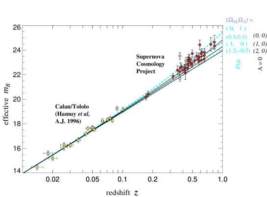
Figure 27: Hubble diagram for the high redshift supernovae found by the SN Cosmology Project. From Ref. [68]. A similar diagram is found by the High Redshift Supernova Project [69]. Both groups conclude that distant supernovae are fainter than expected, and this could be due to an accelerating universe.

This conclusions have been supported by growingly robust observational evidence from distant supernovae. In their quest for the cosmological parameters, astronomers look for distant astrophysical objects that can serve as standard candles to determine the distance to the object from their observed apparent luminosity. A candidate that has recently been exploited with great success is a certain type of supernova explosions at large redshifts, called SN of type Ia. These are white dwarf stars at the end of their life cycle that accrete matter from a companion until they become unstable and violently explode in a natural thermonuclear explosion that out-shines their progenitor galaxy. The intensity of the distant flash varies in time, it takes about three weeks to reach its maximum brightness and then it declines over a period of months. Although the maximum luminosity varies from one supernova to another, depending on their original mass, their environment, etc., there is a pattern: brighter explosions last longer than fainter ones. By studying the characteristic light curves, see Fig. 26, of a reasonably large statistical sample, cosmologists from two competing groups, the Supernova Cosmology Project [68] and the High-redshift Supernova Project [69], are confident that they can use this type of supernova as a standard candle. Since the light coming from some of these rare explosions has travelled for a large fraction of the size of the universe, one expects to be able to infer from their distribution the spatial curvature and the rate of expansion of the universe.

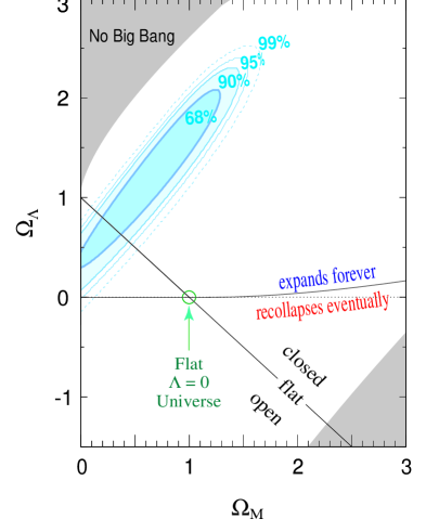
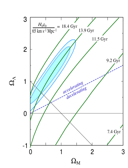
Figure 28: The left figure shows the best-fit confidence regions (68% – 99% c.l.) in the ($\Omega_{\rm M},\,\Omega_{\Lambda}$) plane, for the high redshift supernovae results. The systematic uncertainty is not shown, and would shift the ellipses vertically. Present observations disfavour the Eisntein-de Sitter model (circle) by several standard deviations. The upper-left shaded region represents “bouncing universe” cosmologies with no Big Bang in the past. The lower-right shaded region corresponds to a universe that is younger than the oldest heavy elements, for any value of $h\geq 0.5$. The right figure shows the isochrones of constant $H_{0}t_{0}$, the age of the universe in units of the Hubble time, $H_{0}^{-1}$, with the best-fit 68% and 90% confidence regions in the ($\Omega_{\rm M},\,\Omega_{\Lambda}$) plane. From Ref. [68].

One of the surprises revealed by these observations is that high redshift type Ia supernovae appear fainter than expected for either an open ($\Omega_{\rm M}<1$) or a flat ($\Omega_{\rm M}=1$) universe, see Fig. 27. In fact, the universe appears to be accelerating instead of decelerating, as was expected from the general attraction of matter, see Eq. (26); something seems to be acting as a repulsive force on very large scales. The most natural explanation for this is the presence of a cosmological constant, a diffuse vacuum energy that permeates all space and, as explained above, gives the universe an acceleration that tends to separate gravitationally bound systems from each other. The best-fit results from the Supernova Cosmology Project give a linear combination  $0.8\Omega_{\rm M}-0.6\Omega_{\Lambda}=-0.2\pm 0.1$  $(1\sigma)$, and, for a flat universe ($\Omega_{\rm M}+\Omega_{\Lambda}=1$), the best-fit values for the combined analysis of both groups [68, 69], are

$$\Omega_{\rm M}^{\rm flat} = 0.28^{\ +0.09}_{\ -0.08}\hskip 5.69054pt(1\sigma\ {\rm statistical})\ ^{\ +0.05}_{\ -0.04}\ ({\rm identified\ systematics})\,,$$ (92)

$$\Omega_{\Lambda}^{\rm flat} = 0.72^{\ +0.08}_{\ -0.09}\hskip 5.69054pt(1\sigma\ {\rm statistical})\ ^{\ +0.04}_{\ -0.05}\ ({\rm identified\ systematics})\,.$$ (93)

However, one may think that it is still premature to conclude that the universe is indeed accelerating, because of possibly large systematic errors inherent to most cosmological measurements, and in particular to observations of supernovae at large redshifts. There has been attempts to find crucial systematic effects like evolution, chemical composition dependence, reddening by dust, etc. in the supernovae observations that would invalidate the claims, but none of them are now considered as a serious threat. Perhaps the most critical one today seems to be sampling effects, since the luminosities of the high-redshift supernovae ($z\sim 0.5-1.0$) are all measured relative to the same set of local supernovae ($z<0.3$). Hence, absolute calibrations, completeness levels, and any other systematic effects related to both data sets are critical. For instance, the intense efforts to search for high-redshift objects have led to the peculiar situation where the nearby sample, which is used for calibration, is now smaller than the distant one. Further searches, already underway, for increasing the nearby supernovae sample will provide an important check.

Moreover, there are bounds on a cosmological constant that come from the statistics of gravitational lensing, with two different methods. Gravitational lensing can be due to various accumulations of matter along the line of sight to the distant light sources. The first method uses the abundance of multiply imaged sources like quasars, lensed by intervening galaxies. The probability of finding a lensed image is directly proportional to the number of galaxies (lenses) along the path and thus to the distance to the source. This distance, for fixed $H_{0}$, increases dramatically for a large value of the cosmological constant: the age of the universe and the distance to the galaxy become large for $\Omega_{\Lambda}\neq 0$ because the universe has been expanding for a longer time; therefore, more lenses are predicted for $\Omega_{\Lambda}>0$. Using this method, an upper limit of

$$\Omega_{\Lambda}<0.75\hskip 28.45274pt(95\%\ {\rm c.l.})$$ (94)

has recently been obtained [70], marginally consistent with the supernovae results, but there are caveats to this powerful method due to uncertainties in the number density and lensing cross section of the lensing galaxies as well as the distant quasars. A second method is lensing by massive clusters of galaxies, which produces widely separated lensed images of quasars and distorted images of background galaxies. The observed statistics, when compared with numerical simulations, rule out the $\Omega_{\rm M}=1$ models and set an upper bound on the cosmological constant, $\Omega_{\Lambda}<0.7$, see Ref. [47]. However, this limit is very sensitive to the resolution of the numerical simulations, which are currently improving.

3.4 The spatial curvature $\Omega_{K}$

As we will discuss in detail in Section 4.4, observations of the two-point correlation function of temperature anisotropies in the microwave background provide a crucial test for the spatial curvature of the universe. From those observations one can tell whether the photons that left the last scattering surface, at redshift $z=1100$, have travelled in straight lines, like in a flat universe, or in curved paths, like in an open one. Very recent observations made by the balloon experiment BOOMERANG suggest that the universe is indeed spatially flat ($\Omega_{K}=0$) with about 10% accuracy [71],

$$\Omega_{0}=\Omega_{\rm M}+\Omega_{\Lambda}=1.0\pm 0.1\hskip 28.45274pt(95\%\ {\rm c.l.})$$ (95)

These measuremnts are bound to be improved in the near future, by both balloon experiments and by the Microwave Anisotropy Probe (MAP) satellite, to be launched by NASA at the end of year 2000 [72]. Furthermore, with the launch in 2007 of Planck satellite [73] we will be able to determine $\Omega_{0}$ with 1% accuracy.

3.5 The age of the universe $t_{0}$

The universe must be older than the oldest objects it contains. Those are believed to be the stars in the oldest clusters in the Milky Way, globular clusters. The most reliable ages come from the application of theoretical models of stellar evolution to observations of old stars in globular clusters. For about 30 years, the ages of globular clusters have remained reasonable stable, at about 15 Gyr [74]. However, recently these ages have been revised downward [75].

During the 1980s and 1990s, the globular cluster age estimates have improved as both new observations have been made with CCDs, and since refinements to stellar evolution models, including opacities, consideration of mixing, and different chemical abundances have been incorporated [76]. From the theory side, uncertainties in globular cluster ages come from uncertainties in convection models, opacities, and nuclear reaction rates. From the observational side, uncertainties arise due to corrections for dust and chemical composition. However, the dominant source of systematic errors in the globular cluster age is the uncertainty in the cluster distances. Fortunately, the Hipparcos satellite recently provided geometric parallax measurements for many nearby old stars with low metallicity, typical of glubular clusters, thus allowing for a new calibration of the ages of stars in globular clusters, leading to a downward revision to $10-13$ Gyr [76]. Moreover, there were very few stars in the Hipparcos catalog with both small parallax erros and low metal abundance. Hence, an increase in the sample size could be critical in reducing the statatistical uncertaintites for the calibration of the globular cluster ages. There are already proposed two new parallax satellites, NASA’s Space Interferometry Mission (SIM) and ESA’s mission, called GAIA, that will give 2 or 3 orders of magnitude more accurate parallaxes than Hipparcos, down to fainter magnitude limits, for several orders of magnitude more stars. Until larger samples are available, however, distance errors are likely to be the largest source of systematic uncertainty to the globular cluster age [21].

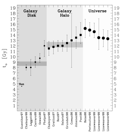
Figure 29: The recent estimates of the age of the universe and that of the oldest objects in our galaxy. The last three points correspond to the combined analysis of 8 different measurements, for $h=$ 0.64, 0.68 and 7.2, which indicates a relatively weak dependence on $h$. The age of the Sun is accurately known and is included for reference. Error bars indicate 1$\sigma$ limits. The averages of the ages of the Galactic Halo and Disk are shaded in gray. Note that there isn’t a single age estimate more than 2$\sigma$ away from the average. The result $t_{0}>t_{\rm gal}$ is logically inevitable, but the standard EdS model does not satisfy this unless $h<0.55$. From Ref. [77].

The supernovae groups can also determine the age of the universe from their high redshift observations. Figure 28 shows that the confidence regions in the $(\Omega_{\rm M},\Omega_{\Lambda})$ plane are almost parallel to the contours of constant age. For any value of the Hubble constant less than $H_{0}=70$ km/s/Mpc, the implied age of the universe is greater than 13 Gyr, allowing enough time for the oldest stars in globular clusters to evolve [76]. Integrating over $\Omega_{\rm M}$ and $\Omega_{\Lambda}$, the best fit value of the age in Hubble-time units is $H_{0}t_{0}=0.93\pm 0.06$ or equivalently $t_{0}=14.1\pm 1.0\ (0.65\,h^{-1})$ Gyr [68]. The age would be somewhat larger in a flat universe: $H_{0}t_{0}^{\rm flat}=0.96^{\ +0.09}_{\ -0.07}$ or, equivalently, [68]

$$t_{0}^{\rm flat}=14.4^{\ +1.4}_{\ -1.1}\hskip 5.69054pt(0.65\,h^{-1})\ {\rm Gyr}\,.$$ (96)

Furthermore, a combination of 8 independent recent measurements: CMB anisotropies, type Ia SNe, cluster mass-to-light ratios, cluster abundance evolution, cluster baryon fraction, deuterium-to-hidrogen ratios in quasar spectra, double-lobed radio sources and the Hubble constant, can be used to determine the present age of the universe [77]. The result is shown in Fig. 29, compared to other recent determinations. The best fit value for the age of the universe is, according to this analysis, $t_{0}=13.4\pm 1.6$ Gyr, about a billion years younger than other recent estimates [77].

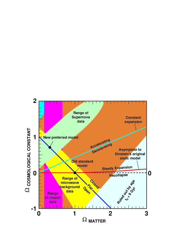
Figure 30: The concordance region. The sum  $\Omega_{\rm M}+\Omega_{\Lambda}$ gives the total cosmic energy content and determines the geometry of space-time, whether spatially flat, open or closed. Their difference,  $\Omega_{\rm M}/2-\Omega_{\Lambda}$, characterizes the relative strength of expansion and gravity, and determines how the expansion rate changes with time, whether accelerating or decelerating. Furthermore, a balance between the two densities determines the fate of the universe, whether it will expand forever or recollapse. These three effects have been probed by recent observations, from large scale structure (cluster data), temperature anisotropies (microwave background data) and the universe expansion (supernova data). Surprisingly enough, at present all observations seem to lie within a naroow region in parameter space. The Einstein-de Sitter model is no longer the preferred one. The best model today is a flat model with a third of the energy density in the form of non-relativistic matter and two thirds in the form of vacuum energy or a cosmological constant. From Ref. [78].

We can summarize this Section by showing the region in parameter space where we stand nowadays, thanks to the recent cosmological observations. We have plotted that region in Fig. 30. One could also superimpose the contour lines corresponding to equal $t_{0}H_{0}$ lines, as a cross check. It is extraordinary that only in the last few months we have been able to reduce the concordance region to where it stands today, where all the different observations seem to converge. There are still many uncertainties, mainly systematic; however, those are quickly decreasing and becoming predominantly statistical. In the near future, with precise observations of the anisotropies in the microwave background temperature and polarization, to be discussed in Section 4.4, we will be able to reduce those uncertainties to the level of one percent. This is the reason why cosmologists are so excited and why it is claimed that we live in the Golden Age of Cosmology.

4 THE INFLATIONARY PARADIGM

The hot Big Bang theory is nowadays a very robust edifice, with many independent observational checks: the expansion of the universe; the abundance of light elements; the cosmic microwave background; a predicted age of the universe compatible with the age of the oldest objects in it, and the formation of structure via gravitational collapse of initially small inhomogeneities. Today, these observations are confirmed to within a few percent accuracy, and have helped establish the hot Big Bang as the preferred model of the universe. All the physics involved in the above observations is routinely tested in the laboratory (atomic and nuclear physics experiments) or in the solar system (general relativity).

However, this theory leaves a range of crucial questions unanswered, most of which are initial conditions’ problems. There is the reasonable assumption that these cosmological problems will be solved or explained by new physical principles at high energies, in the early universe. This assumption leads to the natural conclusion that accurate observations of the present state of the universe may shed light onto processes and physical laws at energies above those reachable by particle accelerators, present or future. We will see that this is a very optimistic approach indeed, and that there are many unresolved issues related to those problems. However, there might be in the near future reasons to be optimistic.

4.1 Shortcomings of Big Bang Cosmology

The Big Bang theory could not explain the origin of matter and structure in the universe; that is, the origin of the matter–antimatter asymmetry, without which the universe today would be filled by a uniform radiation continuosly expanding and cooling, with no traces of matter, and thus without the possibility to form gravitationally bound systems like galaxies, stars and planets that could sustain life. Moreover, the standard Big Bang theory assumes, but cannot explain, the origin of the extraordinary smoothness and flatness of the universe on the very large scales seen by the microwave background probes and the largest galaxy catalogs. It cannot explain the origin of the primordial density perturbations that gave rise to cosmic structures like galaxies, clusters and superclusters, via gravitational collapse; the quantity and nature of the dark matter that we believe holds the universe together; nor the origin of the Big Bang itself.

A summary [79] of the problems that the Big Bang theory cannot explain is:

• The global structure of the universe.

  - Why is the universe so close to spatial flatness?

  - Why is matter so homogeneously distributed on large scales?

• The origin of structure in the universe.

  - How did the primordial spectrum of density perturbations originate?

• The origin of matter and radiation.

  - Where does all the energy in the universe come from?

  - What is the nature of the dark matter in the universe?

  - How did the matter-antimatter asymmetry arise?

• The initial singularity.

  - Did the universe have a beginning?

  - What is the global structure of the universe beyond our observable patch?

Let me discuss one by one the different issues:

4.1.1 The Flatness Problem

The Big Bang theory assumes but cannot explain the extraordinary spatial flatness of our local patch of the universe. In the general FRW metric (2) the parameter $K$ that characterizes spatial curvature is a free parameter. There is nothing in the theory that determines this parameter a priori. However, it is directly related, via the Friedmann equation (8), to the dynamics, and thus the matter content, of the universe,

$$K={8\pi G\over 3}\rho a^{2}-H^{2}a^{2}\ =\ {8\pi G\over 3}\rho a^{2}\Big{(}{\Omega-1\over\Omega}\Big{)}\,.$$ (97)

We can therefore define a new variable,

$$x\equiv{\Omega-1\over\Omega}={{\rm const.}\over\rho a^{2}}\,,$$ (98)

whose time evolution is given by

$$x^{\prime}={dx\over dN}=(1+3\omega)\,x\,,$$ (99)

where $N=\ln(a/a_{i})$ characterizes the number of $e$-folds of universe expansion ($dN=Hdt$) and where we have used Eq. (38) for the time evolution of the total energy, $\rho a^{3}$, which only depends on the barotropic ratio $\omega$. It is clear from Eq. (99) that the phase-space diagram $(x,x^{\prime})$ presents an unstable critical (saddle) point at $x=0$ for $\omega>-1/3$, i.e. for the radiation ($\omega=1/3$) and matter ($\omega=0$) eras. A small perturbation from $x=0$ will drive the system towards $x=\pm\infty$. Since we know the universe went through both the radiation era (because of primordial nucleosynthesis) and the matter era (because of structure formation), tiny deviations from $\Omega=1$ would have grown since then, such that today

$$x_{0}={\Omega_{0}-1\over\Omega_{0}}=x_{\rm in}\,\Big{(}{T_{\rm in}\over T_{\rm eq}}\Big{)}^{2}(1+z_{\rm eq})\,.$$ (100)

In order that today’s value be in the range $0.1<\Omega_{0}<1.2$, or $x_{0}\approx{\cal O}(1)$, it is required that at, say, primordial nucleosynthesis ($T_{{}_{\rm NS}}\simeq 10^{6}\,T_{\rm eq}$)  its value be

$$\Omega(t_{{}_{\rm NS}})=1\pm 10^{-15}\,,$$ (101)

which represents a tremendous finetuning. Perhaps the universe indeed started with such a peculiar initial condition, but it is epistemologically more satisfying if we give a fundamental dynamical reason for the universe to have started so close to spatial flatness. These arguments were first used by Robert Dicke in the 1960s, much before inflation. He argued that the most natural initial condition for the spatial curvature should have been the Planck scale curvature, ${}^{(3)}\!R=6K/l_{\rm P}^{2}$, where the Planck length is $l_{\rm P}=(\hbar G/c^{3})^{1/2}=1.62\times 10^{-33}$ cm, that is, 60 orders of magnitude smaller than the present size of the universe, $a_{0}=1.38\times 10^{28}$ cm. A universe with this immense curvature would have collapsed within a Planck time, $t_{\rm P}=(\hbar G/c^{5})^{1/2}=5.39\times 10^{-44}$ s, again 60 orders of magnitude smaller than the present age of the universe, $t_{0}=4.1\times 10^{17}$ s. Therefore, the flatness problem is also related to the Age Problem, why is it that the universe is so old and flat when, under ordinary circumstances (based on the fundamental scale of gravity) it should have lasted only a Planck time and reached a size of order the Planck length? As we will see, inflation gives a dynamical reason to such a peculiar initial condition.

4.1.2 The Homogeneity Problem

An expanding universe has particle horizons, that is, spatial regions beyond which causal communication cannot occur. The horizon distance can be defined as the maximum distance that light could have travelled since the origin of the universe [8],

$$d_{\rm H}(t)\equiv a(t)\int_{0}^{t}{dt^{\prime}\over a(t^{\prime})}\sim H^{-1}(t)\,,$$ (102)

which is proportional to the Hubble scale. For instance, at the beginning of nucleosynthesis the horizon distance is a few light-seconds, but grows linearly with time and by the end of nucleosynthesis it is a few light-minutes, i.e. a factor 100 larger, while the scale factor has increased only a factor of 10. The fact that the causal horizon increases faster, $d_{\rm H}\sim t$, than the scale factor, $a\sim t^{1/2}$, implies that at any given time the universe contains regions within itself that, according to the Big Bang theory, were never in causal contact before. For instance, the number of causally disconnected regions at a given redshift $z$ present in our causal volume today, $d_{\rm H}(t_{0})\equiv a_{0}$, is

$$N_{\rm CD}(z)\sim\left({a(t)\over d_{\rm H}(t)}\right)^{3}\simeq(1+z)^{3/2}\,,$$ (103)

which, for the time of decoupling, is of order $N_{\rm CD}(z_{\rm dec})\sim 10^{5}\gg 1$.

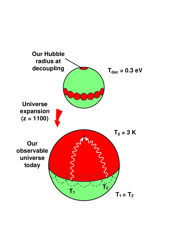
Figure 31: Perhaps the most acute problem of the Big Bang theory is explaining the extraordinary homogeneity and isotropy of the microwave background, see Fig. 6. At the time of decoupling, the volume that gave rise to our present universe contained many causally disconnected regions (top figure). Today we observe a blackbody spectrum of photons coming from those regions and they appear to have the same temperature, $T_{1}=T_{2}$, to one part in $10^{5}$. Why is the universe so homogeneous? This constitutes the so-called horizon problem, which is spectacularly solved by inflation. From Ref. [80, 78].

This phenomenon is particularly acute in the case of the observed microwave background. Information cannot travel faster than the speed of light, so the causal region at the time of photon decoupling could not be larger than $d_{\rm H}(t_{\rm dec})\sim 3\times 10^{5}$ light years across, or about $1^{\circ}$ projected in the sky today. So why should regions that are separated by more than $1^{\circ}$ in the sky today have exactly the same temperature, to within 10 ppm, when the photons that come from those two distant regions could not have been in causal contact when they were emitted? This constitutes the so-called horizon problem, see Fig. 31, and was first discussed by Robert Dicke in the 1970s as a profound inconsistency of the Big Bang theory.

4.2 Cosmological Inflation

In the 1980s, a new paradigm, deeply rooted in fundamental physics, was put forward by Alan H. Guth [81], Andrei D. Linde [82] and others [83, 84, 85], to address these fundamental questions. According to the inflationary paradigm, the early universe went through a period of exponential expansion, driven by the approximately constant energy density of a scalar field called the inflaton. In modern physics, elementary particles are represented by quantum fields, which resemble the familiar electric, magnetic and gravitational fields. A field is simply a function of space and time whose quantum oscillations are interpreted as particles. In our case, the inflaton field has, associated with it, a large potential energy density, which drives the exponential expansion during inflation, see Fig. 32. We know from general relativity that the density of matter determines the expansion of the universe, but a constant energy density acts in a very peculiar way: as a repulsive force that makes any two points in space separate at exponentially large speeds. (This does not violate the laws of causality because there is no information carried along in the expansion, it is simply the stretching of space-time.)

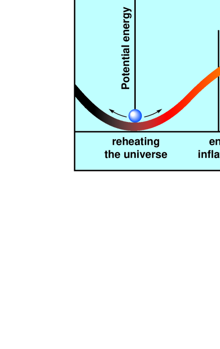
Figure 32: The inflaton field can be represented as a ball rolling down a hill. During inflation, the energy density is approximately constant, driving the tremendous expansion of the universe. When the ball starts to oscillate around the bottom of the hill, inflation ends and the inflaton energy decays into particles. In certain cases, the coherent oscillations of the inflaton could generate a resonant production of particles which soon thermalize, reheating the universe. From Ref. [78].

This superluminal expansion is capable of explaining the large scale homogeneity of our observable universe and, in particular, why the microwave background looks so isotropic: regions separated today by more than $1^{\circ}$ in the sky were, in fact, in causal contact before inflation, but were stretched to cosmological distances by the expansion. Any inhomogeneities present before the tremendous expansion would be washed out. This explains why photons from supposedly causally disconneted regions have actually the same spectral distribution with the same temperature, see Fig. 31.

Moreover, in the usual Big Bang scenario a flat universe, one in which the gravitational attraction of matter is exactly balanced by the cosmic expansion, is unstable under perturbations: a small deviation from flatness is amplified and soon produces either an empty universe or a collapsed one. As we discussed above, for the universe to be nearly flat today, it must have been extremely flat at nucleosynthesis, deviations not exceeding more than one part in $10^{15}$. This extreme fine tuning of initial conditions was also solved by the inflationary paradigm, see Fig. 33. Thus inflation is an extremely elegant hypothesis that explains how a region much, much greater that our own observable universe could have become smooth and flat without recourse to ad hoc initial conditions. Furthermore, inflation dilutes away any “unwanted” relic species that could have remained from early universe phase transitions, like monopoles, cosmic strings, etc., which are predicted in grand unified theories and whose energy density could be so large that the universe would have become unstable, and collapsed, long ago. These relics are diluted by the superluminal expansion, which leaves at most one of these particles per causal horizon, making them harmless to the subsequent evolution of the universe.

Figure 33: The exponential expansion during inflation made the radius of curvature of the universe so large that our observable patch of the universe today appears essentialy flat, analogous (in three dimensions) to how the surface of a balloon appears flatter and flatter as we inflate it to enormous sizes. This is a crucial prediction of cosmological inflation that will be tested to extraordinary accuracy in the next few years. From Ref. [84, 78].

The only thing we know about this peculiar scalar field, the inflaton, is that it has a mass and a self-interaction potential $V(\phi)$ but we ignore everything else, even the scale at which its dynamics determines the superluminal expansion. In particular, we still do not know the nature of the inflaton field itself, is it some new fundamental scalar field in the electroweak symmetry breaking sector, or is it just some effective description of a more fundamental high energy interaction? Hopefully, in the near future, experiments in particle physics might give us a clue to its nature. Inflation had its original inspiration in the Higgs field, the scalar field supposed to be responsible for the masses of elementary particles (quarks and leptons) and the breaking of the electroweak symmetry. Such a field has not been found yet, and its discovery at the future particle colliders would help understand one of the truly fundamental problems in physics, the origin of masses. If the experiments discover something completely new and unexpected, it would automatically affect the idea of inflation at a fundamental level.

4.2.1 Homogeneous scalar field dynamics

In this subsection I will describe the theoretical basis for the phenomenon of inflation. Consider a scalar field $\phi$, a singlet under any given interaction, with an effective potential $V(\phi)$. The Lagrangian for such a field in a curved background is

$${\cal L}_{\rm inf}={1\over 2}\,g^{\mu\nu}\partial_{\mu}\phi\partial_{\nu}\phi-V(\phi)\,,$$ (104)

whose evolution equation in a Friedmann-Robertson-Walker metric (2) and for a homogeneous field $\phi(t)$ is given by

$$\ddot{\phi}+3H\dot{\phi}+V^{\prime}(\phi)=0\,,$$ (105)

where $H$ is the rate of expansion, together with the Einstein equations,

$$H^{2} = {\kappa^{2}\over 3}\Big{(}{1\over 2}\,\dot{\phi}^{2}+V(\phi)\Big{)}\,,$$ (106)

$$\dot{H} = -{\kappa^{2}\over 2}\,\dot{\phi}^{2}\,,$$ (107)

where $\kappa^{2}\equiv 8\pi G$. The dynamics of inflation can be described as a perfect fluid (7) with a time dependent pressure and energy density given by

$$\rho = {1\over 2}\,\dot{\phi}^{2}+V(\phi)\,,$$ (108)

$$p = {1\over 2}\,\dot{\phi}^{2}-V(\phi)\,.$$ (109)

The field evolution equation (105) can then be written as the energy conservation equation,

$$\dot{\rho}+3H(\rho+p)=0\,.$$ (110)

If the potential energy density of the scalar field dominates the kinetic energy, $V(\phi)\gg\dot{\phi}^{2}$, then we see that

$$p\simeq-\rho\hskip 14.22636pt\Rightarrow\hskip 14.22636pt\rho\simeq{\rm const.}\hskip 14.22636pt\Rightarrow\hskip 14.22636ptH(\phi)\simeq{\rm const.}\,,$$ (111)

which leads to the solution

$$a(t)\sim\exp(Ht)\hskip 14.22636pt\Rightarrow\hskip 14.22636pt{\ddot{a}\over a}>0\hskip 14.22636pt{\rm accelerated\ expansion}\,.$$ (112)

Using the definition of the number of $e$-folds, $N=\ln(a/a_{i})$, we see that the scale factor grows exponentially, $a(N)=a_{i}\exp(N)$. This solution of the Einstein equations solves immediately the flatness problem. Recall that the problem with the radiation and matter eras is that $\Omega=1$ ($x=0$) is an unstable critical point in phase-space. However, during inflation, with $p\simeq-\rho\ \Rightarrow\ \omega\simeq-1$, we have that $1+3\omega\geq 0$ and therefore $x=0$ is a stable attractor of the equations of motion, see Eq. (99). As a consequence, what seemed an ad hoc initial condition, becomes a natural prediction of inflation. Suppose that during inflation the scale factor increased $N$ $e$-folds, then

$$x_{0}=x_{\rm in}\,e^{-2N}\,\Big{(}{T_{\rm rh}\over T_{\rm eq}}\Big{)}^{2}(1+z_{\rm eq})\ \simeq\ e^{-2N}\,10^{56}\leq 1\hskip 14.22636pt\Rightarrow\hskip 14.22636ptN\geq 65\,,$$ (113)

where we have assumed that inflation ended at the scale $V_{\rm end}$, and the transfer of the inflaton energy density to thermal radiation at reheating occurred almost instantaneously at the temperature  $T_{\rm rh}\sim V_{\rm end}^{1/4}\sim 10^{15}$ GeV. Note that we can now have initial conditions with a large uncertainty, $x_{\rm in}\simeq 1$, and still have today $x_{0}\simeq 1$, thanks to the inflationary attractor towards $\Omega=1$. This can be understood very easily by realizing that the three curvature evolves during inflation as

$$^{(3)}R={6K\over a^{2}}=\ ^{(3)}\!R_{\rm in}\,e^{-2N}\hskip 14.22636pt\longrightarrow\hskip 14.22636pt0\,,\hskip 14.22636pt{\rm for}\ \ N\gg 1\,.$$ (114)

Therefore, if cosmological inflation lasted over 65 $e$-folds, as most models predict, then today the universe (or at least our local patch) should be exactly flat, see Fig. 33, a prediction that can be tested with great accuracy in the near future and for which already seems to be some evidence from observations of the microwave background [71].

Furthermore, inflation also solves the homogeneity problem in a spectacular way. First of all, due to the superluminal expansion, any inhomogeneity existing prior to inflation will be washed out,

$$\delta_{k}\sim\ \left({k\over aH}\right)^{2}\,\Phi_{k}\hskip 5.69054pt\propto\hskip 5.69054pte^{-2N}\hskip 14.22636pt\longrightarrow\hskip 14.22636pt0\,,\hskip 14.22636pt{\rm for}\ \ N\gg 1\,.$$ (115)

Moreover, since the scale factor grows exponentially, while the horizon distance remains essentially constant, $d_{H}(t)\simeq H^{-1}=$ const., any scale within the horizon during inflation will be stretched by the superluminal expansion to enormous distances, in such a way that at photon decoupling all the causally disconnected regions that encompass our present horizon actually come from a single region during inflation, about 65 $e$-folds before the end. This is the reason why two points separated more than $1^{\circ}$ in the sky have the same backbody temperature, as observed by the COBE satellite: they were actually in causal contact during inflation. There is at present no other proposal known that could solve the homogeneity problem without invoquing an acausal mechanism like inflation.

Finally, any relic particle species (relativistic or not) existing prior to inflation will be diluted by the expansion,

$$\rho_{\rm M} \propto a^{-3}\ \sim\ e^{-3N}\hskip 14.22636pt\longrightarrow\hskip 14.22636pt0\,,\hskip 14.22636pt{\rm for}\ \ N\gg 1\,,$$ (116)

$$\rho_{\rm R} \propto a^{-4}\ \sim\ e^{-4N}\hskip 14.22636pt\longrightarrow\hskip 14.22636pt0\,,\hskip 14.22636pt{\rm for}\ \ N\gg 1\,.$$ (117)

Note that the vacuum energy density $\rho_{v}$ remains constant under the expansion, and therefore, very soon it is the only energy density remaining to drive the expansion of the universe.

4.2.2 The slow-roll approximation

In order to simplify the evolution equations during inflation, we will consider the slow-roll approximation (SRA). Suppose that, during inflation, the scalar field evolves very slowly down its effective potential, then we can define the slow-roll parameters [86],

$$\epsilon \equiv -\,{\dot{H}\over H^{2}}\ =\ {\kappa^{2}\over 2}\,{\dot{\phi}^{2}\over H^{2}}\ \ll\ 1\,,$$ (118)

$$\delta \equiv -\,{\ddot{\phi}\over H\dot{\phi}}\ \ll\ 1\,.$$ (119)

It is easy to see that the condition

$$\epsilon<1\hskip 14.22636pt\Longleftrightarrow\hskip 14.22636pt{\ddot{a}\over a}>0$$ (120)

characterizes inflation: it is all you need for superluminal expansion, i.e. for the horizon distance to grow more slowly than the scale factor, in order to solve the homogeneity problem, as well as for the spatial curvature to decay faster than usual, in order to solve the flatness problem.

The number of $e$-folds during inflation can be written with the help of Eq. (118) as

$$N\ =\ \ln{a_{\rm end}\over a_{i}}\ =\ \int_{t_{i}}^{t_{e}}Hdt\ =\ \int_{\phi_{i}}^{\phi_{e}}{\kappa d\phi\over\sqrt{2\epsilon(\phi)}}\,,$$ (121)

which is an exact expression in terms of $\epsilon(\phi)$.

In the limit given by Eqs. (118), the evolution equations (105) and (106) become

$$H^{2}\Big{(}1-{\epsilon\over 3}\Big{)} \simeq H^{2}\ =\ {\kappa^{2}\over 3}\,V(\phi)\,,$$ (122)

$$3H\dot{\phi}\,\Big{(}1-{\delta\over 3}\Big{)} \simeq 3H\dot{\phi}\ =\ -\,V^{\prime}(\phi)\,.$$ (123)

Note that this corresponds to a reduction of the dimensionality of phase-space from two to one dimensions, $H(\phi,\dot{\phi})\rightarrow H(\phi)$. In fact, it is possible to prove a theorem, for single-field inflation, which states that the slow-roll approximation is an attractor of the equations of motion, and thus we can always evaluate the inflationary trajectory in phase-space within the SRA, therefore reducing the number of initial conditions to just one, the initial value of the scalar field. If $H(\phi)$ only depends on $\phi$, then $H^{\prime}(\phi)=-\kappa^{2}\dot{\phi}/2$ and we can rewrite the slow-roll parameters (118) as

$$\epsilon = {2\over\kappa^{2}}\left({H^{\prime}(\phi)\over H(\phi)}\right)^{2}\ \simeq\ {1\over 2\kappa^{2}}\left({V^{\prime}(\phi)\over V(\phi)}\right)^{2}\ \ll\ 1\,,$$ (124)

$$\delta = {2\over\kappa^{2}}\,{H^{\prime\prime}(\phi)\over H(\phi)}\ \simeq\ {1\over\kappa^{2}}\,{V^{\prime\prime}(\phi)\over V(\phi)}-{1\over 2\kappa^{2}}\left({V^{\prime}(\phi)\over V(\phi)}\right)^{2}\ \equiv\ \eta-\epsilon\ \ll\ 1\,.$$ (125)

The last expression defines the new slow-roll parameter $\eta$, not to be confused with conformal time (see next Section). The number of $e$-folds can also be rewritten in this approximation as

$$N\ =\ \kappa^{2}\,\int_{\phi_{i}}^{\phi_{e}}{V(\phi)\,d\phi\over V^{\prime}(\phi)}\,,$$ (126)

a very useful expression for evaluating $N$ for a given effective scalar potential $V(\phi)$.

4.3 The origin of density perturbations

If cosmological inflation made the universe so extremely flat and homogeneous, where did the galaxies and clusters of galaxies come from? One of the most astonishing predictions of inflation, one that was not even expected, is that quantum fluctuations of the inflaton field are stretched by the exponential expansion and generate large-scale perturbations in the metric. Inflaton fluctuations are small wave packets of energy that, according to general relativity, modify the space-time fabric, creating a whole spectrum of curvature perturbations. The use of the word spectrum here is closely related to the case of light waves propagating in a medium: a spectrum characterizes the amplitude of each given wavelength. In the case of inflation, the inflaton fluctuations induce waves in the space-time metric that can be decomposed into different wavelengths, all with approximately the same amplitude, that is, corresponding to a scale-invariant spectrum. These patterns of perturbations in the metric are like fingerprints that unequivocally characterize a period of inflation. When matter fell in the troughs of these waves, it created density perturbations that collapsed gravitationally to form galaxies, clusters and superclusters of galaxies, with a spectrum that is also scale invariant. Such a type of spectrum was proposed in the early 1970s (before inflation) by Harrison and Zel’dovich [17], to explain the distribution of galaxies and clusters of galaxies on very large scales in our observable universe. Perhaps the most interesting aspect of structure formation is the possibility that the detailed knowledge of what seeded galaxies and clusters of galaxies will allow us to test the idea of inflation.

4.3.1 Gauge invariant perturbation theory

Until now we have considered only the unperturbed FRW metric described by a scale factor $a(t)$ and a homogeneous scalar field $\phi(t)$,

$$ds^{2} = a^{2}(\eta)[d\eta^{2}-\gamma_{ij}\,dx^{i}dx^{j}]\,,$$ (127)

$$\phi = \phi(\eta)\,,$$ (128)

where $\eta=\int dt/a(t)$ is the conformal time, under which the background equations of motion can be written as

$${\cal H}^{2} = {\kappa^{2}\over 3}\left({1\over 2}{\phi^{\prime}}^{2}+a^{2}V(\phi)\right)\,,$$ (129)

$${\cal H}^{\prime}-{\cal H}^{2} = {\kappa^{2}\over 2}{\phi^{\prime}}^{2}\,,$$ (130)

$$\phi^{\prime\prime}+2{\cal H}\phi^{\prime}+a^{2}V^{\prime}(\phi) = 0\,,$$ (131)

where ${\cal H}=aH$ and $\phi^{\prime}=a\dot{\phi}$.

During inflation, the quantum fluctuations of the scalar field will induce metric perturbations which will backreact on the scalar field. Let us consider, in linear perturbation theory, the most general line element with both scalar and tensor metric perturbations [87], together with the scalar field perturbations

$$ds^{2} = a^{2}(\eta)\left[(1+2A)d\eta^{2}-2B_{|i}dx^{i}d\eta-\Big{\{}(1+2{\cal R})\gamma_{ij}+2E_{|ij}+2h_{ij}\Big{\}}dx^{i}dx^{j}\right]\,,$$ (132)

$$\phi = \phi(\eta)+\delta\phi(\eta,x^{i})\,.$$ (133)

The indices $\{i,j\}$ label the three-dimensional spatial coordinates with metric $\gamma_{ij}$, and the $|i$ denotes covariant derivative with respect to that metric. The gauge invariant tensor perturbation $h_{ij}$ corresponds to a transverse traceless gravitational wave, $\nabla^{i}h_{ij}=h^{i}_{i}=0$. The four scalar perturbations $(A,B,{\cal R},E)$ are gauge dependent functions of $(\eta,x^{i})$. Under a general coordinate (gauge) transformation [87, 88]

$$\tilde{\eta}=\eta+\xi^{0}(\eta,x^{i})\,,$$ (134)

$$\tilde{x}^{i}=x^{i}+\gamma^{ij}\xi_{|j}(\eta,x^{i})\,,$$ (135)

with arbitrary functions $(\xi^{0},\xi)$, the scalar and tensor perturbations transform, to linear order, as

$$\tilde{A}=A-{\xi^{0}}^{\prime}-{\cal H}\xi^{0}\,,\hskip 28.45274pt\tilde{B}=B+\xi^{0}-\xi^{\prime}\,,$$ (136)

$$\tilde{\cal R}={\cal R}-{\cal H}\xi^{0}\,,\hskip 54.06006pt\tilde{E}=E-\xi\,,$$ (137)

$$\hskip 85.35826pt\tilde{h}_{ij}=h_{ij}\,,$$ (138)

where a prime denotes derivative with respect to conformal time. It is possible to construct, however, two gauge-invariant gravitational potentials [87, 88],

$$\Phi=A+(B-E^{\prime})^{\prime}+{\cal H}(B-E^{\prime})\,,$$ (139)

$$\Psi={\cal R}+{\cal H}(B-E^{\prime})\,,$$ (140)

which are related through the perturbed Einstein equations,

$$\Phi = \Psi\,,$$ (141)

$${k^{2}-3K\over a^{2}}\Psi = {\kappa^{2}\over 2}\delta\rho\,,$$ (142)

where $\delta\rho$ is the gauge-invariant density perturbation, and the latter expression is nothing but the Poisson equation for the gravitational potential, written in relativistic form.

During inflation, the energy density is given in terms of a scalar field, and thus the gauge-invariant equations for the perturbations on comoving hypersurfaces (constant energy density hypersurfaces) are

$$\Phi^{\prime\prime}+3{\cal H}\Phi^{\prime}+({\cal H}^{\prime}+{\cal H}^{2})\Phi = {\kappa^{2}\over 2}[\phi^{\prime}\delta\phi^{\prime}-a^{2}V^{\prime}(\phi)\delta\phi]\,,$$ (143)

$$-\nabla^{2}\Phi+3{\cal H}\Phi^{\prime}+({\cal H}^{\prime}+{\cal H}^{2})\Phi = -{\kappa^{2}\over 2}[\phi^{\prime}\delta\phi^{\prime}+a^{2}V^{\prime}(\phi)\delta\phi]\,,$$ (144)

$$\Phi^{\prime}+{\cal H}\Phi = {\kappa^{2}\over 2}\phi^{\prime}\delta\phi\,,$$ (145)

$$\delta\phi^{\prime\prime}+2{\cal H}\delta\phi^{\prime}-\nabla^{2}\delta\phi = 4\phi^{\prime}\Phi^{\prime}-2a^{2}V^{\prime}(\phi)\Phi-a^{2}V^{\prime\prime}(\phi)\delta\phi\,.$$ (146)

This system of equations seem too difficult to solve at first sight. However, there is a gauge invariant combination of variables that allows one to find exact solutions. Let us define [88]

$$u\equiv a\delta\phi+z\Phi\,,$$ (147)

$$z\equiv a{\phi^{\prime}\over{\cal H}}\,.$$ (148)

Under this redefinition, the above equations simplify enormously to just three independent equations,

$$u^{\prime\prime}-\nabla^{2}u-{z^{\prime\prime}\over z}u=0\,,$$ (149)

$$\nabla^{2}\Phi={\kappa^{2}\over 2}{{\cal H}\over a^{2}}(zu^{\prime}-z^{\prime}u)\,,$$ (150)

$$\Big{(}{a^{2}\Phi\over{\cal H}}\Big{)}^{\prime}={\kappa^{2}\over 2}zu\,.$$ (151)

From Equation (149) we can find a solution $u(z)$, which substituted into (151) can be integrated to give $\Phi(z)$, and together with $u(z)$ allow us to obtain $\delta\phi(z)$.

4.3.2 Quantum Field Theory in curved space-time

Until now we have treated the perturbations as classical, but we should in fact consider the perturbations $\Phi$ and $\delta\phi$ as quantum fields. Note that the perturbed action for the scalar mode $u$ can be written as

$$\delta S={1\over 2}\int d^{3}x\,d\eta\,\Big{[}(u^{\prime})^{2}-(\nabla u)^{2}+{z^{\prime\prime}\over z}u^{2}\Big{]}\,.$$ (152)

In order to quantize the field $u$ in the curved background defined by the metric (127), we can write the operator

$$\hat{u}(\eta,{\bf x})=\int{d^{3}{\bf k}\over(2\pi)^{3/2}}\Big{[}u_{k}(\eta)\,\hat{a}_{\bf k}\,e^{i{\bf k}\cdot{\bf x}}+u_{k}^{*}(\eta)\,\hat{a}_{\bf k}^{\dagger}\,e^{-i{\bf k}\cdot{\bf x}}\Big{]}\,,$$ (153)

where the creation and annihilation operators satisfy the commutation relation of bosonic fields, and the scalar field’s Fock space is defined through the vacuum condition,

$$[\hat{a}_{\bf k},\hat{a}_{{\bf k}^{\prime}}^{\dagger}] = \delta^{3}({\bf k-k}^{\prime})\,,$$ (154)

$$\hat{a}_{\bf k}|0\rangle = 0\,.$$ (155)

Note that we are not assuming that the inflaton is a fundamental scalar field, but that is can be written as a quantum field with its commutation relations (as much as a pion can be described as a quantum field).

The equations of motion for each mode $u_{k}(\eta)$ are decoupled in linear perturbation theory,

$$u^{\prime\prime}_{k}+\Big{(}k^{2}-{z^{\prime\prime}\over z}\Big{)}u_{k}=0\,.$$ (156)

The ratio $z^{\prime\prime}/z$ acts like a time-dependent potential for this Schrödinger like equation. In order to find exact solutions to the mode equation, we will use the slow-roll parameters (118), see Ref. [86]

$$\epsilon=1-{{\cal H}^{\prime}\over{\cal H}^{2}}={\kappa^{2}\over 2}{z^{2}\over a^{2}}\,,$$ (157)

$$\delta=1-{\phi^{\prime\prime}\over{\cal H}\phi^{\prime}}=1+\epsilon-{z^{\prime}\over{\cal H}z}\,.$$ (158)

In terms of these parameters, the conformal time and the effective potential for the $u_{k}$ mode can be written as

$$\eta={-1\over{\cal H}}+\int{\epsilon da\over a{\cal H}}\,,$$ (159)

$${z^{\prime\prime}\over z}={\cal H}^{2}[(1+\epsilon-\delta)(2-\delta)+{\cal H}^{-1}(\epsilon^{\prime}-\delta^{\prime})]\,.$$ (160)

Note that the slow-roll parameters, (157) and (158), can be taken as constant, to order $\epsilon^{2}$,

$$\epsilon^{\prime}=2{\cal H}\,\epsilon(\epsilon-\delta)={\cal O}(\epsilon^{2})\,,$$ (161)

$$\delta^{\prime}={\cal H}\,\delta\Big{(}\epsilon+\delta+{\stackrel{{\scriptstyle\dots}}{{\phi}}\over H\ddot{\phi}}\Big{)}={\cal O}(\epsilon^{2})\,.$$ (162)

In that case, for constant parameters, we can write

$$\eta={-1\over{\cal H}}{1\over 1-\epsilon}\,,$$ (163)

$${z^{\prime\prime}\over z}={1\over\eta^{2}}\Big{(}\nu^{2}-{1\over 4}\Big{)}\,, \hskip 14.22636pt{\rm where}\hskip 19.91692pt\nu={1+\epsilon-\delta\over 1-\epsilon}+{1\over 2}\,.$$ (164)

We are now going to search for approximate solutions of the mode equation (156), where the effective potential (160) is of order $z^{\prime\prime}/z\simeq 2{\cal H}^{2}$ in the slow-roll approximation. In quasi-de Sitter there is a characteristic scale given by the (event) horizon size or Hubble scale during inflation, $H^{-1}$. There will be modes $u_{k}$ with physical wavelengths much smaller than this scale, $k/a\gg H$, that are well within the de Sitter horizon and therefore do not feel the curvature of space-time. On the other hand, there will be modes with physical wavelengths much greater than the Hubble scale, $k/a\ll H$. In these two asymptotic regimes, the solutions can be written as

$$u_{k}={1\over\sqrt{2k}}\,e^{-ik\eta}\hskip 28.45274ptk\gg aH\,,$$ (165)

$$u_{k}=C_{1}\,z\hskip 56.9055ptk\ll aH\,.$$ (166)

In the limit $k\gg aH$ the modes behave like ordinary quantum modes in Minkowsky space-time, appropriately normalized, while in the opposite limit, $u/z$ becomes constant on superhorizon scales. For approximately constant slow-roll parameters one can find exact solutions to (156), with the effective potential given by (164), that interpolate between the two asymptotic solutions,

$$u_{k}(\eta)={\sqrt{\pi}\over 2}\,e^{i(\nu+{1\over 2}){\pi\over 2}}\,(-\eta)^{1/2}\,H_{\nu}^{{}_{(1)}}(-k\eta)\,,$$ (167)

where $H_{\nu}^{{}_{(1)}}(z)$ is the Hankel function of the first kind [89], and $\nu$ is given by (164) in terms of the slow-roll parameters. In the limit $k\eta\to 0$, the solution becomes

$$|u_{k}|={2^{\nu-{3\over 2}}\over\sqrt{2k}}\,{\Gamma(\nu)\over\Gamma({3\over 2})}\,(-k\eta)^{{1\over 2}-\nu}\equiv{C(\nu)\over\sqrt{2k}}\,\Big{(}{k\over aH}\Big{)}^{\nu-{1\over 2}}\,,$$ (168)

$$C(\nu)=2^{\nu-{3\over 2}}\,{\Gamma(\nu)\over\Gamma({3\over 2})}\,(1-\epsilon)^{\nu-{1\over 2}}\ \simeq 1\hskip 28.45274pt{\rm for}\hskip 14.22636pt\epsilon,\delta\ll 1\,.$$ (169)

We can now compute $\Phi$ and $\delta\phi$ from the super-Hubble-scale mode solution (166), for $k\ll aH$. Substituting into Eq. (151), we find

$$\Phi=C_{1}\,\Big{(}1-{{\cal H}\over a^{2}}\,\int a^{2}d\eta\Big{)}+C_{2}\,{{\cal H}\over a^{2}}\,,$$ (170)

$$\delta\phi={C_{1}\over a^{2}}\,\int a^{2}d\eta-{C_{2}\over a^{2}}\,.$$ (171)

The term proportional to $C_{1}$ corresponds to the growing solution, while that proportional to $C_{2}$ corresponds to the decaying solution, which can soon be ignored. These quantities are gauge invariant but evolve with time outside the horizon, during inflation, and before entering again the horizon during the radiation or matter eras. We would like to write an expression for a gauge invariant quantity that is also constant for superhorizon modes. Fortunately, in the case of adiabatic perturbations, there is such a quantity:

$$\zeta\equiv\Phi+{1\over\epsilon{\cal H}}\,(\Phi^{\prime}+{\cal H}\Phi)={u\over z}\,,$$ (172)

which is constant, see Eq. (166), for $k\ll aH$. In fact, this quantity $\zeta$ is identical, for superhorizon modes, to the gauge invariant curvature metric perturbation ${\cal R}_{c}$ on comoving (constant energy density) hypersurfaces, see Ref. [87, 90],

$$\zeta={\cal R}_{c}+{1\over\epsilon{\cal H}^{2}}\,\nabla^{2}\Phi\,.$$ (173)

Using Eq. (150) we can write the evolution equation for $\zeta={u\over z}$ as  $\zeta^{\prime}={1\over\epsilon{\cal H}}\,\nabla^{2}\Phi$, which confirms that $\zeta$ is constant for (adiabatic) superhorizon modes, $k\ll aH$. Therefore, we can evaluate the Newtonian potential $\Phi_{k}$ when the perturbation reenters the horizon during radiation/matter eras in terms of the curvature perturbation ${\cal R}_{k}$ when it left the Hubble scale during inflation,

$$\Phi_{k}=\Big{(}1-{{\cal H}\over a^{2}}\,\int a^{2}d\eta\Big{)}\,{\cal R}_{k}={3+3\omega\over 5+3\omega}\,{\cal R}_{k}=\hskip 2.84526pt\left\{\begin{array}[]{cl}{2\over 3}\,{\cal R}_{k}&\hskip 14.22636pt{\rm radiation\hskip 5.69054ptera}\,,\\[8.53581pt] {3\over 5}\,{\cal R}_{k}&\hskip 14.22636pt{\rm matter\hskip 5.69054ptera}\,.\end{array}\right.$$ (174)

Let us now compute the tensor or gravitational wave metric perturbations generated during inflation. The perturbed action for the tensor mode can be written as

$$\delta S={1\over 2}\int d^{3}x\,d\eta\,{a^{2}\over 2\kappa^{2}}\Big{[}(h_{ij}^{\prime})^{2}-(\nabla h_{ij})^{2}\Big{]}\,,$$ (175)

with the tensor field $h_{ij}$ considered as a quantum field,

$$\hat{h}_{ij}(\eta,{\bf x})=\int{d^{3}{\bf k}\over(2\pi)^{3/2}}\sum_{\lambda=1,2}\Big{[}h_{k}(\eta)\,e_{ij}({\bf k},\lambda)\,\hat{a}_{\bf k,\lambda}\,e^{i{\bf k}\cdot{\bf x}}+h.c.\Big{]}\,,$$ (176)

where $e_{ij}({\bf k},\lambda)$ are the two polarization tensors, satisfying symmetric, transverse and traceless conditions

$$e_{ij}=e_{ji}\,,\hskip 14.22636ptk^{i}e_{ij}=0\,,\hskip 14.22636pte_{ii}=0\,,$$ (177)

$$e_{ij}(-{\bf k},\lambda)=e_{ij}^{*}({\bf k},\lambda)\,,\hskip 14.22636pt\sum_{\lambda}e_{ij}^{*}({\bf k},\lambda)e^{ij}({\bf k},\lambda)=4\,,$$ (178)

while the creation and annihilation operators satisfy the usual commutation relation of bosonic fields, Eq. (154). We can now redefine our gauge invariant tensor amplitude as

$$v_{k}(\eta)={a\over\sqrt{2}\kappa}\,h_{k}(\eta)\,,$$ (179)

which satisfies the following evolution equation, decoupled for each mode $v_{k}(\eta)$ in linear perturbation theory,

$$v^{\prime\prime}_{k}+\Big{(}k^{2}-{a^{\prime\prime}\over a}\Big{)}v_{k}=0\,.$$ (180)

The ratio $a^{\prime\prime}/a$ acts like a time-dependent potential for this Schrödinger like equation, analogous to the term $z^{\prime\prime}/z$ for the scalar metric perturbation. For constant slow-roll parameters, the potential becomes

$${a^{\prime\prime}\over a}=2{\cal H}^{2}\Big{(}1-{\epsilon\over 2}\Big{)}={1\over\eta^{2}}\Big{(}\mu^{2}-{1\over 4}\Big{)}\,,$$ (181)

$$\mu={1\over 1-\epsilon}+{1\over 2}\,.$$ (182)

We can solve equation (180) in the two asymptotic regimes,

$$v_{k}={1\over\sqrt{2k}}\,e^{-ik\eta}\hskip 28.45274ptk\gg aH\,,$$ (183)

$$v_{k}=C\,a\hskip 62.59596ptk\ll aH\,.$$ (184)

In the limit $k\gg aH$ the modes behave like ordinary quantum modes in Minkowsky space-time, appropriately normalized, while in the opposite limit, the metric perturbation $h_{k}$ becomes constant on superhorizon scales. For constant slow-roll parameters one can find exact solutions to (180), with effective potential given by (181), that interpolate between the two asymptotic solutions. These are identical to Eq. (167) except for the substitution $\nu\to\mu$. In the limit $k\eta\to 0$, the solution becomes

$$|v_{k}|={C(\mu)\over\sqrt{2k}}\,\Big{(}{k\over aH}\Big{)}^{\mu-{1\over 2}}\,.$$ (185)

Since the mode $h_{k}$ becomes constant on superhorizon scales, we can evaluate the tensor metric perturbation when it reentered during the radiation or matter era directly in terms of its value during inflation.

4.3.3 Power spectrum of scalar and tensor metric perturbations

Not only do we expect to measure the amplitude of the metric perturbations generated during inflation and responsible for the anisotropies in the CMB and density fluctuations in LSS, but we should also be able to measure its power spectrum, or two-point correlation function in Fourier space. Let us consider first the scalar metric perturbations ${\cal R}_{k}$, which enter the horizon at $a=k/H$. Its correlator is given by [86]

$$\langle 0|{\cal R}_{k}^{*}{\cal R}_{k^{\prime}}|0\rangle={|u_{k}|^{2}\over z^{2}}\,\delta^{3}({\bf k-k^{\prime}})\equiv{{\cal P}_{\cal R}(k)\over 4\pi k^{3}}\,(2\pi)^{3}\,\delta^{3}({\bf k-k^{\prime}})\,,$$ (186)

$${\cal P}_{\cal R}(k)={k^{3}\over 2\pi^{2}}\,{|u_{k}|^{2}\over z^{2}}={\kappa^{2}\over 2\epsilon}\,\Big{(}{H\over 2\pi}\Big{)}^{2}\,\Big{(}{k\over aH}\Big{)}^{3-2\nu}\equiv A_{S}^{2}\,\Big{(}{k\over aH}\Big{)}^{n-1}\,,$$ (187)

where we have used  ${\cal R}_{k}=\zeta_{k}={u_{k}\over z}$ and Eq. (168). This last equation determines the power spectrum in terms of its amplitude at horizon-crossing, $A_{S}$, and a tilt,

$$n-1\equiv{d\ln{\cal P}_{\cal R}(k)\over d\ln k}=3-2\nu=2\Big{(}{\delta-2\epsilon\over 1-\epsilon}\Big{)}\simeq 2\eta-6\epsilon\,,$$ (188)

see Eqs. (124), (125). Note from this equation that it is possible, in principle, to obtain from inflation a scalar tilt which is either positive ($n>1$) or negative ($n<1$). Furthermore, depending on the particular inflationary model [91], we can have significant departures from scale invariance.

Let us consider now the tensor (gravitational wave) metric perturbation, which enter the horizon at  $a=k/H$,

$$\sum_{\lambda}\langle 0|h^{*}_{k,\lambda}h_{k^{\prime},\lambda}|0\rangle=4\,{2\kappa^{2}\over a^{2}}\,|v_{k}|^{2}\delta^{3}({\bf k-k^{\prime}})\equiv{{\cal P}_{g}(k)\over 4\pi k^{3}}\,(2\pi)^{3}\,\delta^{3}({\bf k-k^{\prime}})\,,$$ (189)

$${\cal P}_{g}(k)=8\kappa^{2}\,\Big{(}{H\over 2\pi}\Big{)}^{2}\,\Big{(}{k\over aH}\Big{)}^{3-2\mu}\equiv A_{T}^{2}\,\Big{(}{k\over aH}\Big{)}^{n_{T}}\,,$$ (190)

where we have used Eqs. (179) and (185). Therefore, the power spectrum can be approximated by a power-law expression, with amplitude $A_{T}$ and tilt

$$n_{T}\equiv{d\ln{\cal P}_{g}(k)\over d\ln k}=3-2\mu=-\Big{(}{2\epsilon\over 1-\epsilon}\Big{)}\simeq-2\epsilon<0\,,$$ (191)

which is always negative. In the slow-roll approximation, $\epsilon\ll 1$, the tensor power spectrum is scale invariant.

4.4 The anisotropies of the microwave background

The metric fluctuations generated during inflation are not only responsible for the density perturbations that gave rise to galaxies via gravitational collapse, but one should also expect to see such ripples in the metric as temperature anisotropies in the cosmic microwave background, that is, minute deviations in the temperature of the blackbody spectrum when we look at different directions in the sky. Such anisotropies had been looked for ever since Penzias and Wilson’s discovery of the CMB, but had eluded all detection, until COBE satellite discovered them in 1992, see Fig. 6. The reason why they took so long to be discovered was that they appear as perturbations in temperature of only one part in $10^{5}$. Soon after COBE, other groups quickly confirmed the detection of temperature anisotropies at around 30 $\mu$K, at higher multipole numbers or smaller angular scales. There are at this moment dozens of ground and balloon-borne experiments analysing the anisotropies in the microwave background with angular resolutions from $10^{\circ}$ to a few arc minutes in the sky, see Fig. 34.

4.4.1 Acoustic oscillations in the plasma

The physics of the CMB anisotropies is relatively simple [92]. The universe just before recombination is a very tightly coupled fluid, due to the large electromagnetic Thomson cross section (54). Photons scatter off charged particles (protons and electrons), and carry energy, so they feel the gravitational potential associated with the perturbations imprinted in the metric during inflation. An overdensity of baryons (protons and neutrons) does not collapse under the effect of gravity until it enters the causal Hubble radius. The perturbation continues to grow until radiation pressure opposes gravity and sets up acoustic oscillations in the plasma, very similar to sound waves. Since overdensities of the same size will enter the Hubble radius at the same time, they will oscillate in phase. Moreover, since photons scatter off these baryons, the acoustic oscillations occur also in the photon field and induces a pattern of peaks in the temperature anisotropies in the sky, at different angular scales, see Fig. 34.

There are three different effects that determine the temperature anisotropies we observe in the CMB. First, gravity: photons fall in and escape off gravitational potential wells, characterized by $\Phi$ in the comoving gauge, and as a consequence their frequency is gravitationally blue- or red-shifted, $\delta\nu/\nu=\Phi$. If the gravitational potential is not constant, the photons will escape from a larger or smaller potential well than they fell in, so their frequency is also blue- or red-shifted, a phenomenon known as the Rees-Sciama effect. Second, pressure: photons scatter off baryons which fall into gravitational potential wells and the two competing forces create acoustic waves of compression and rarefaction. Finally, velocity: baryons accelerate as they fall into potential wells. They have minimum velocity at maximum compression and rarefaction. That is, their velocity wave is exactly $90^{\circ}$ off-phase with the acoustic waves. These waves induce a Doppler effect on the frequency of the photons.

The temperature anisotropy induced by these three effects is therefore given by [92]

$${\delta T\over T}({\bf r})=\Phi({\bf r},t_{\rm dec})+2\int_{t_{\rm dec}}^{t_{0}}\dot{\Phi}({\bf r},t)dt\ +\ {1\over 3}{\delta\rho\over\rho}\ -\ {{\bf r}\cdot{\bf v}\over c}\,.$$ (192)

Metric perturbations of different wavelengths enter the horizon at different times. The largest wavelengths, of size comparable to our present horizon, are entering now. There are perturbations with wavelengths comparable to the size of the horizon at the time of last scattering, of projected size about $1^{\circ}$ in the sky today, which entered precisely at decoupling. And there are perturbations with wavelengths much smaller than the size of the horizon at last scattering, that entered much earlier than decoupling, all the way to the time of radiation-matter equality, which have gone through several acoustic oscillations before last scattering. All these perturbations of different wavelengths leave their imprint in the CMB anisotropies.

The baryons at the time of decoupling do not feel the gravitational attraction of perturbations with wavelength greater than the size of the horizon at last scattering, because of causality. Perturbations with exactly that wavelength are undergoing their first contraction, or acoustic compression, at decoupling. Those perturbations induce a large peak in the temperature anisotropies power spectrum, see Fig. 34. Perturbations with wavelengths smaller than these will have gone, after they entered the Hubble scale, through a series of acoustic compressions and rarefactions, which can be seen as secondary peaks in the power spectrum. Since the surface of last scattering is not a sharp discontinuity, but a region of $\Delta z\sim 100$, see Fig. 4, there will be scales for which photons, travelling from one energy concentration to another, will erase the perturbation on that scale, similarly to what neutrinos or HDM do for structure on small scales. That is the reason why we don’t see all the acoustic oscillations with the same amplitude, but in fact they decay exponentialy towards smaller angular scales, an effect known as Silk damping, due to photon diffusion [93, 92].

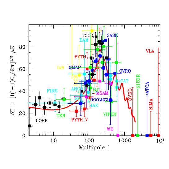
Figure 34: There are at present dozens of ground and balloon-borne experiments looking at the microwave background temperature anisotropies with angular resolutions from $10^{\circ}$ to a few arc minutes in the sky, corresponding to multipole numbers $l=2-3000$. Present observations suggest the existence of a peak in the angular distribution, as predicted by inflation. The theoretical curve (thick line) illustrates a particular model which fits the data. From Ref. [94].

4.4.2 The Sachs-Wolfe effect

The anisotropies corresponding to large angular scales are only generated via gravitational red-shift and density perturbations through the Einstein equations, $\delta\rho/\rho=-2\Phi$ for adiabatic perturbations; we can ignore the Doppler contribution, since the perturbation is non-causal. In that case, the temperature anisotropy in the sky today is given by [95]

$${\delta T\over T}(\theta,\phi)={1\over 3}\Phi(\eta_{\rm LS})\,Q(\eta_{0},\theta,\phi)+2\int_{\eta_{\rm LS}}^{\eta_{0}}dr\,\Phi^{\prime}(\eta_{0}-r)\,Q(r,\theta,\phi)\,,$$ (193)

where $\eta_{0}$ is the coordinate distance to the last scattering surface, i.e. the present conformal time, while $\eta_{\rm LS}\simeq 0$ determines that comoving hypersurface. The above expression is known as the Sachs-Wolfe effect [95], and contains two parts, the intrinsic and the Integrated Sachs-Wolfe (ISW) effect, due to integration along the line of sight of time variations in the gravitational potential.

In linear perturbation theory, the scalar metric perturbations can be separated into $\Phi(\eta,{\bf x})\equiv\Phi(\eta)\,Q({\bf x})$, where $Q({\bf x})$ are the scalar harmonics, eigenfunctions of the Laplacian in three dimensions, $\nabla^{2}Q_{klm}(r,\theta,\phi)=-k^{2}\,Q_{klm}(r,\theta,\phi)$. These functions have the general form [96]

$$Q_{klm}(r,\theta,\phi)=\Pi_{kl}(r)\,Y_{lm}(\theta,\phi)\,,$$ (194)

where $Y_{lm}(\theta,\phi)$ are the usual spherical harmonics [89].

In order to compute the temperature anisotropy associated with the Sachs-Wolfe effect, we have to know the evolution of the metric perturbation during the matter era,

$$\Phi^{\prime\prime}+3{\cal H}\,\Phi^{\prime}+a^{2}\Lambda\,\Phi-2K\,\Phi=0\,.$$ (195)

In the case of a flat universe without cosmological constant, the Newtonian potential remains constant during the matter era and only the intrinsic SW effect contributes to $\delta T/T$. In case of a non-vanishing $\Lambda$, since its contribution is negligible in the past, see Eq. (25), most of the photon’s trajectory towards us is unperturbed, and the only difference with respect to the $\Lambda=0$ case is an overall factor [66]. We will consider here the approximation $\Phi={\rm const}$. during the matter era and ignore that factor, see Ref. [97].

In a flat universe, the radial part of the eigenfunctions (194) can be written as [96]

$$\Pi_{kl}(r)=\sqrt{2\over\pi}\,k\,j_{l}(kr)\,,$$ (196)

where $j_{l}(z)$ are the spherical Bessel functions [89]. The growing mode solution of the metric perturbation that left the Hubble scale during inflation contributes to the temperature anisotropies on large scales (193) as

$${\delta T\over T}(\theta,\phi)\ =\ {1\over 3}\Phi(\eta_{\rm LS})\,Q\ =\ {1\over 5}\,{\cal R}\,Q(\eta_{0},\theta,\phi)\ \equiv\ \sum_{l=2}^{\infty}\sum_{m=-l}^{l}\,a_{lm}\,Y_{lm}(\theta,\phi)\,,$$ (197)

where we have used the fact that at reentry (at the surface of last scattering) the gauge invariant Newtonian potential $\Phi$ is related to the curvature perturbation ${\cal R}$ at Hubble-crossing during inflation, see Eq. (174); and we have expanded $\delta T/T$ in spherical harmonics.

We can now compute the two-point correlation function or angular power spectrum, $C(\theta)$, of the CMB anisotropies on large scales, defined as an expansion in multipole number,

$$C(\theta)=\left\langle{\delta T\over T}^{*}\!({\bf n}){\delta T\over T}({\bf n}^{\prime})\right\rangle_{{\bf n}\cdot{\bf n}^{\prime}=\cos\theta}={1\over 4\pi}\sum_{l=2}^{\infty}(2l+1)\,C_{l}\,P_{l}(\cos\theta)\,,$$ (198)

where $P_{l}(z)$ are the Legendre polynomials [89], and we have averaged over different universe realizations. Since the coefficients $a_{lm}$ are isotropic (to first order), we can compute the $C_{l}=\langle|a_{lm}|^{2}\rangle$ as

$$C_{l}^{(S)}={4\pi\over 25}\,\int_{0}^{\infty}\,{dk\over k}\,{\cal P}_{\cal R}(k)\,j_{l}^{2}(k\eta_{0})\,,$$ (199)

where we have used Eqs. (197) and (186). In the case of scalar metric perturbation produced during inflation, the scalar power spectrum at reentry is given by ${\cal P}_{\cal R}(k)=A_{S}^{2}(k\eta_{0})^{n-1}$, in the power-law approximation, see Eq. (187). In that case, one can integrate (199) to give

$$C_{l}^{(S)}={2\pi\over 25}\,A_{S}^{2}\,{\Gamma[{3\over 2}]\,\Gamma[1-{n-1\over 2}]\,\Gamma[l+{n-1\over 2}]\over\Gamma[{3\over 2}-{n-1\over 2}]\,\Gamma[l+2-{n-1\over 2}]}\,,$$ (200)

$${l(l+1)\,C_{l}^{(S)}\over 2\pi}={A_{S}^{2}\over 25}\ =\ {\rm constant}\,,\hskip 28.45274pt{\rm for}\hskip 8.53581ptn=1\,.$$ (201)

This last expression corresponds to what is known as the Sachs-Wolfe plateau, and is the reason why the coefficients $C_{l}$ are always plotted multiplied by $l(l+1)$, see Fig. 34.

Tensor metric perturbations also contribute with an approximately constant angular power spectrum, $l(l+1)C_{l}$. The Sachs-Wolfe effect for a gauge invariant tensor perturbation is given by [95]

$${\delta T\over T}(\theta,\phi)=\int_{\eta_{\rm LS}}^{\eta_{0}}dr\,h^{\prime}(\eta_{0}-r)\,Q_{rr}(r,\theta,\phi)\,,$$ (202)

where $Q_{rr}$ is the $rr$-component of the tensor harmonic along the line of sight [96]. The tensor perturbation $h$ during the matter era satisfies the following evolution equation

$$h^{\prime\prime}_{k}+3{\cal H}\,h^{\prime}_{k}+(k^{2}+2K)\,h_{k}=0\,,$$ (203)

which depends on the wavenumber $k$, contrary to what happens with the scalar modes, see Eq. (195). For a flat ($K=0$) universe, the solution to this equation is  $h_{k}(\eta)=h\,G_{k}(\eta)$, where $h$ is the constant tensor metric perturbation at horizon crossing and $G_{k}(\eta)=3\,j_{1}(k\eta)/k\eta$, normalized so that $G_{k}(0)=1$ at the surface of last scattering. The radial part of the tensor harmonic $Q_{rr}$ in a flat universe can be written as [96]

$$Q^{rr}_{kl}(r)=\left[{(l-1)l(l+1)(l+2)\over\pi k^{2}}\right]^{1/2}\,{j_{l}(kr)\over r^{2}}\,.$$ (204)

The tensor angular power spectrum can finally be expressed as

$$C_{l}^{(T)}={9\pi\over 4}\,(l-1)l(l+1)(l+2)\,\int_{0}^{\infty}\,{dk\over k}\,{\cal P}_{g}(k)\,I_{kl}^{2}\,,$$ (205)

$$I_{kl}=\int_{0}^{x_{0}}\,dx\,{j_{2}(x_{0}-x)j_{l}(x)\over(x_{0}-x)x^{2}}\,,$$ (206)

where $x\equiv k\eta$, and ${\cal P}_{g}(k)$ is the primordial tensor spectrum (190). For a scale invariant spectrum, $n_{T}=0$, we can integrate (205) to give [98]

$$l(l+1)\,C_{l}^{(T)}={\pi\over 36}\Big{(}1+{48\pi^{2}\over 385}\Big{)}\,A_{T}^{2}\,B_{l}\,,$$ (207)

with  $B_{l}=(1.1184,0.8789,\dots,1.00)$  for $l=2,3,\dots,30$. Therefore, $l(l+1)\,C_{l}^{(T)}$ also becomes constant for large $l$. Beyond $l\sim 30$, the Sachs-Wolfe expression is not a good approximation and the tensor angular power spectrum decays very quickly at large $l$, see Fig.40.

4.4.3 The consistency relation

In spite of the success of inflation in predicting a homogeneous and isotropic background on which to imprint a scale-invariant spectrum of inhomogeneities, it is difficult to test the idea of inflation. A CMB cosmologist before the 1980s would have argued that ad hoc initial conditions could have been at the origin of the homogeneity and flatness of the universe on large scales, while a LSS cosmologist would have agreed with Harrison and Zel’dovich that the most natural spectrum needed to explain the formation of structure was a scale-invariant spectrum. The surprise was that inflation incorporated an understanding of both the globally homogeneous and spatially flat background, and the approximately scale-invariant spectrum of perturbations in the same formalism. But that could have been a coincidence, and is not epistemologically testable.

What is unique to inflation is the fact that inflation determines not just one but two primordial spectra, corresponding to the scalar (density) and tensor (gravitational waves) metric perturbations, from a single continuous function, the inflaton potential $V(\phi)$. In the slow-roll approximation, one determines, from $V(\phi)$, two continuous functions, ${\cal P}_{\cal R}(k)$ and ${\cal P}_{g}(k)$, that in the power-law approximation reduces to two amplitudes, $A_{S}$ and $A_{T}$, and two tilts, $n$ and $n_{T}$. It is clear that there must be a relation between the four parameters. Indeed, one can see from Eqs. (207) and (201) that the ratio of the tensor to scalar contribution to the angular power spectrum is proportional to the tensor tilt [86],

$$R\equiv{C_{l}^{(T)}\over C_{l}^{(S)}}={25\over 9}\Big{(}1+{48\pi^{2}\over 385}\Big{)}\,2\epsilon\simeq-2\pi\,n_{T}\,.$$ (208)

This is a unique prediction of inflation, which could not have been postulated a priori by any cosmologist. If we finally observe a tensor spectrum of anisotropies in the CMB, or a stochastic gravitational wave background in laser interferometers like LIGO or VIRGO [99], with sufficient accuracy to determine their spectral tilt, one might have some chance to test the idea of inflation, via the consistency relation (208). For the moment, observations of the microwave background anisotropies suggest that the Sachs-Wolfe plateau exists, see Fig. 34, but it is still premature to determine the tensor contribution. Perhaps in the near future, from the analysis of polarization as well as temperature anisotropies, with the CMB satellites MAP and Planck, we might have a chance of determining the validity of the consistency relation.

Assuming that the scalar contribution dominates over the tensor on large scales, i.e. $R\ll 1$, one can actually give a measure of the amplitude of the scalar metric perturbation from the observations of the Sachs-Wolfe plateau in the angular power spectrum [97],

$$\left[{l(l+1)\,C_{l}^{(S)}\over 2\pi}\right]^{1/2} = {A_{S}\over 5}\ =\ (1.03\pm 0.07)\times 10^{-5}\,,$$ (209)

$$n = 1.02\pm 0.12\,.$$ (210)

These measurements can be used to normalize the primordial spectrum and determine the parameters of the model of inflation [91]. In the near future these parameters will be determined with much better accuracy, as described in Section 4.4.5.

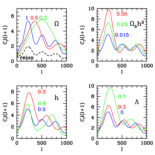
Figure 35: Theoretical predictions for CMB temperature angular power spectra as a function of multipole number $l$ for models with primordial adiabatic perturbations. Each graph shows the effect of a variation in one of these parameters. From Ref. [100].

4.4.4 The acoustic peaks

The Sachs-Wolfe plateau is a distinctive feature of Fig. 34. These observations confirm the existence of a primordial spectrum of scalar (density) perturbations on all scales, otherwise the power spectrum would have started from zero at $l=2$. However, we see that the spectrum starts to rise around $l=20$ towards the first acoustic peak, where the SW approximation breaks down and the above formulae are no longer valid.

As mentioned above, the first peak in the photon distribution corresponds to overdensities that have undergone half an oscillation, that is, a compression, and appear at a scale associated with the size of the horizon at last scattering, about $1^{\circ}$ projected in the sky today. Since photons scatter off baryons, they will also feel the acoustic wave and create a peak in the correlation function. The height of the peak is proportional to the amount of baryons: the larger the baryon content of the universe, the higher the peak. The position of the peak in the power spectrum depends on the geometrical size of the particle horizon at last scattering. Since photons travel along geodesics, the projected size of the causal horizon at decoupling depends on whether the universe is flat, open or closed. In a flat universe the geodesics are straight lines and, by looking at the angular scale of the first acoustic peak, we would be measuring the actual size of the horizon at last scattering. In an open universe, the geodesics are inward-curved trajectories, and therefore the projected size on the sky appears smaller. In this case, the first acoustic peak should occur at higher multipoles or smaller angular scales. On the other hand, for a closed universe, the first peak occurs at smaller multipoles or larger angular scales. The dependence of the position of the first acoustic peak on the spatial curvature can be approximately given by [92]

$$l_{\rm peak}\simeq 220\,\Omega_{0}^{-1/2}\,,$$ (211)

where $\Omega_{0}=\Omega_{\rm M}+\Omega_{\Lambda}=1-\Omega_{K}$. Present observations, specially the ones of the Mobile Anisotropy Telescope (MAT) in Cerro Tololo, Chile, which produced two data sets, TOCO97 and TOCO98 [101], and the recent balloon-borne experiment BOOMERANG [71], suggest that the peak is between $l=180$ and 250 at 95% c.l., with an amplitude $\delta T=80\pm 10\ \mu$K, and therefore the universe is most probably flat, see Fig. 36, and Ref. [102]. In particular, these measuremts determine that

$$0.85\leq\Omega_{0}\leq 1.25\hskip 14.22636pt(68\%\ {\rm c.l.})$$ (212)

That is, the universe is flat, within 10% uncertainty, which is much better than we could ever do before. In the near future we will measure $\Omega_{0}$ to within 1%, with the new microwave anisotropy satellites.

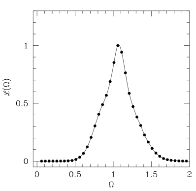
Figure 36: The left figure shows the power spectrum of the BOOMERANG experiment with 6 arcminute pixelization. The solid curve is a marginally closed model with $(\Omega_{\rm B},\Omega_{\rm M},\Omega_{\Lambda},n,h)=(0.05,0.26,0.75,0.95,0.7)$. The dotted curve is Standard CDM with $(0.05,0.95,0.0,1.0,0.65)$. The dashed curves are open and closed models with fixed $\Omega_{0}=\Omega_{\rm M}+\Omega_{\Lambda}=0.66$ and 1.55, respectively. The right figure shows the likelihood function of $\Omega_{0}$ normalized to unity at the peak, after marginalizing over the $\Omega_{\rm M}-\Omega_{\Lambda}$ direction. From Ref. [71].

At the moment there is not enough information at small angular scales, or large multipole numbers, to determine the existence or not of the secondary acoustic peaks. These peaks should occur at harmonics of the first one, but are typically much lower because of Silk damping. Since the amplitude and position of the primary and secondary peaks are directly determined by the sound speed (and, hence, the equation of state) and by the geometry and expansion of the universe, they can be used as a powerful test of the density of baryons and dark matter, and other cosmological parameters, see Fig. 35.

By looking at these patterns in the anisotropies of the microwave background, cosmologists can determine not only the cosmological parameters, see Fig. 35, but also the primordial spectrum of density perturbations produced during inflation. It turns out that the observed temperature anisotropies are compatible with a scale-invariant spectrum, see Eq. (210), as predicted by inflation. This is remarkable, and gives very strong support to the idea that inflation may indeed be responsible for both the CMB anisotropies and the large-scale structure of the universe. Different models of inflation have different specific predictions for the fine details associated with the spectrum generated during inflation. It is these minute differences that will allow cosmologists to differentiate between alternative models of inflation and discard those that do not agree with observations. However, most importantly, perhaps, the pattern of anisotropies predicted by inflation is completely different from those predicted by alternative models of structure formation, like cosmic defects: strings, vortices, textures, etc. These are complicated networks of energy density concentrations left over from an early universe phase transition, analogous to the defects formed in the laboratory in certain kinds of liquid crystals when they go through a phase transition. The cosmological defects have spectral properties very different from those generated by inflation. That is why it is so important to launch more sensitive instruments, and with better angular resolution, to determine the properties of the CMB anisotropies.

Figure 37: The left figure shows a simulation of the temperature anisotropies predicted by a generic model of inflation, as would be seen by a satellite like COBE with angular resolution of $7^{\circ}$. The right figure shows the same, but with a satellite like Planck, with a resolution 100 times better. From Ref. [73].

4.4.5 The new microwave anisotropy satellites, MAP and Planck

The large amount of information encoded in the anisotropies of the microwave background is the reason why both NASA and the European Space Agency have decided to launch two independent satellites to measure the CMB temperature and polarization anisotropies to unprecendented accuracy. The Microwave Anisotropy Probe [72] will be launched by NASA at the end of 2000, and Planck [73] is expected in 2007.

As we have emphasized before, the fact that these anisotropies have such a small amplitude allow for an accurate calculation of the predicted anisotropies in linear perturbation theory. A particular cosmological model is characterized by a dozen or so parameters: the rate of expansion, the spatial curvature, the baryon content, the cold dark matter and neutrino contribution, the cosmological constant (vacuum energy), the reionization parameter (optical depth to the last scattering surface), and various primordial spectrum parameters like the amplitude and tilt of the adiabatic and isocurvature spectra, the amount of gravitational waves, non-Gaussian effects, etc. All these parameters can now be fed into a fast code called CMBFAST [103] that computes the predicted temperature and polarization anisotropies to 1% accuracy, and thus can be used to compare with observations.

These two satellites will improve both the sensitivity, down to $\mu$K, and the resolution, down to arc minutes, with respect to the previous COBE satellite, thanks to large numbers of microwave horns of various sizes, positioned at specific angles, and also thanks to recent advances in detector technology, with high electron mobility transistor amplifiers (HEMTs) for frequencies below 100 GHz and bolometers for higher frequencies. The primary advantage of HEMTs is their ease of use and speed, with a typical sensitivity of 0.5 mKs^1/2, while the advantage of bolometers is their tremendous sensitivity, better than 0.1 mKs^1/2, see Ref. [104]. For instance, to appreciate the difference, compare the resolution in the temperature anisotropies that COBE and Planck would observe for the same simulated sky in Fig. 37. This will allow cosmologists to extract information from around 3000 multipoles! Since most of the cosmological parameters have specific signatures in the height and position of the first few acoustic peaks, the higher the resolution, the more peaks one is expected to see, and thus the better the accuracy with which one will be able to measure those parameters, see Table 1. As an example of the kind of data that these two satellites will be able to provide, see Fig. 38, which compares the present observational status with that which will become available around 2008.

Figure 38: The predicted angular power spectrum of temperature anisotropies, compared with the present data, see Fig. 34, binned into 16 logarithmic intervals in multipole number between $l=2$ and $l=1000$. The right figure gives an estimate of the accuracy with which the power spectrum will be measured by Planck. It is only limited by cosmic variance on all the angular scales relevant to primary anisotropies. From Ref. [105].

Although the satellite probes were designed for the accurate measurement of the CMB temperature anisotropies, there are other experiments, like balloon-borne and ground interferometers, which will probably accomplish the same results with similar resolution (in the case of MAP), before the satellites start producing their own results [104]. Probably the most important objective of the future satellites will be the measurement of the CMB polarization anisotropies, yet to be discovered. These anisotropies are predicted by models of structure formation and are expected to arise at the level of microKelvin sensitivities, where the new satellites are aiming at. The complementary information contained in the polarization anisotropies will provide much more stringent constraints on the cosmological parameters than from the temperature anisotropies alone. In particular, the curl-curl component of the polarization power spectra is nowadays the only means we have to determine the tensor (gravitational wave) contribution to the metric perturbations responsible for temperature anisotropies, see Fig. 39. If such a component is found, one could constraint very precisely the model of inflation from its spectral properties, specially the tilt [100].

Figure 39: Theoretical predictions for the four non-zero CMB temperature-polarization spectra as a function of multipole moment. The dotted curves are the predictions for a COBE-normalized scalar perturbation from an inflationary model with no reionization and no gravitational waves for $h=0.65$, $\Omega_{\rm B}h^{2}=0.024$, and $\Lambda=0$. The solid curves are the corresponding predictions if the COBE anisotropy were entirely due to a stochastic gravitational wave background with a flat scale-invariant spectrum (with the same cosmological parameters). The panel for $C_{l}^{\rm CC}$ contains no dotted curve because scalar perturbations produce no curl component of the polarization vector. From Ref. [100].

physical quantity	symbol	present range	MAP	Planck
luminous matter	$\Omega_{\rm lum}h^{2}$	$0.001-0.005$	$-$	$-$
baryonic matter	$\Omega_{\rm B}h^{2}$	$0.01-0.03$	5%	0.6%
cold dark matter	$\Omega_{\rm M}h^{2}$	$0.2-1.0$	10%	0.6%
hot dark matter	$\Omega_{\nu}h^{2}$	$0-0.3$	5%	2%
cosmological constant	$\Omega_{\Lambda}h^{2}$	$0-0.8$	8%	0.5%
spatial curvature	$\Omega_{0}h^{2}$	$0.2-1.5$	4%	0.7%
rate of expansion	$h$	$0.4-0.8$	11%	2%
age of the universe	$t_{0}$	$11-17$ Gyr	10%	2%
spectral amplitude	$Q_{\rm rms}$	$20-30\ \mu$K	0.5%	0.1%
spectral tilt	$n_{{}_{\rm S}}$	$0.5-1.5$	3%	0.5%
tensor-scalar ratio	$r_{\rm ts}$	$0-1.0$	25%	10%
reionization	$\tau$	$0.01-1.0$	20%	15%

Table 1: The parameters of the standard cosmological model. The standard model of cosmology has around 12 different parameters, needed to describe the background space-time, the matter content and the spectrum of density perturbations. We include here the present range of the most relevant parameters, and the percentage error with which the microwave background probes MAP and Planck (without polarization) will be able to determine them in the near future. The rate of expansion is in units of $H_{0}=100\,h$ km/s/Mpc.

4.5 From metric perturbations to large scale structure

If inflation is responsible for the metric perturbations that gave rise to the temperature anisotropies observed in the microwave background, then the primordial spectrum of density inhomogeneities induced by the same metric perturbations should also be responsible for the present large scale structure [106]. This simple connection allows for more stringent tests on the inflationary paradigm for the generation of metric perturbations, since it relates the large scales (of order the present horizon) with the smallest scales (on galaxy scales). This provides a very large lever arm for the determination of primordial spectra parameters like the tilt, the nature of the perturbations, whether adiabatic or isocurvature, the geometry of the universe, as well as its matter and energy content, whether CDM, HDM or mixed CHDM.

4.5.1 The galaxy power spectrum

As metric perturbations enter the causal horizon during the radiation or matter era, they create density fluctuations via gravitational attraction of the potential wells. The density contrast $\delta$ can be deduced from the Einstein equations in linear perturbation theory, see Eq. (142),

$$\delta_{k}\equiv{\delta\rho_{k}\over\rho}=\left({k\over aH}\right)^{2}\,{2\over 3}\,\Phi_{k}=\left({k\over aH}\right)^{2}\,{2+2\omega\over 5+3\omega}\,{\cal R}_{k}\,,$$ (213)

where we have assumed $K=0$, and used Eq. (174). From this expression one can compute the power spectrum, at horizon crossing, of matter density perturbations induced by inflation, see Eq. (186),

$$P(k)=\langle|\delta_{k}|^{2}\rangle=A\,\left({k\over aH}\right)^{n}\,,$$ (214)

with $n$ given by the scalar tilt (188), $n=1+2\eta-6\epsilon$. This spectrum reduces to a Harrison-Zel’dovich spectrum (57) in the slow-roll approximation:  $\eta,\,\epsilon\ll 1$.

Since perturbations evolve after entering the horizon, the power spectrum will not remain constant. For scales entering the horizon well after matter domination ($k^{-1}\gg k^{-1}_{\rm eq}\simeq 81$ Mpc), the metric perturbation has not changed significantly, so that ${\cal R}_{k}({\rm final})={\cal R}_{k}({\rm initial})$. Then Eq. (213) determines the final density contrast in terms of the initial one. On smaller scales, there is a linear transfer function $T(k)$, which may be defined as [86]

$${\cal R}_{k}({\rm final})=T(k)\,{\cal R}_{k}({\rm initial})\,.$$ (215)

To calculate the transfer function one has to specify the initial condition with the relative abundance of photons, neutrinos, baryons and cold dark matter long before horizon crossing. The most natural condition is that the abundances of all particle species are uniform on comoving hypersurfaces (with constant total energy density). This is called the adiabatic condition, because entropy is conserved independently for each particle species $X$, i.e. $\delta\rho_{X}=\dot{\rho}_{X}\delta t$, given a perturbation in time from a comoving hypersurface, so

$${\delta\rho_{X}\over\rho_{X}+p_{X}}={\delta\rho_{Y}\over\rho_{Y}+p_{Y}}\,,$$ (216)

where we have used the energy conservation equation for each species, $\dot{\rho}_{X}=-3H(\rho_{X}+p_{X})$, valid to first order in perturbations. It follows that each species of radiation has a common density contrast $\delta_{r}$, and each species of matter has also a common density contrast $\delta_{m}$, with the relation  $\delta_{m}={3\over 4}\delta_{r}$.

Within the horizon, the density perturbation amplitude evolves according to the following equation, see Ref. [86],

$$H^{-2}\ddot{\delta}_{k}+[2-3(2\omega-c_{s}^{2})]\,H^{-1}\dot{\delta}_{k}-{3\over 2}\,(1-6c_{s}^{2}+8\omega-3\omega^{2})\,\delta_{k}=-\left({k\over aH}\right)^{2}{\delta p_{k}\over\rho}\,,$$ (217)

where  $\omega=p/\rho$  is the barotropic ratio, and  $c_{s}^{2}=\dot{p}/\dot{\rho}$  is the speed of sound of the fluid.

Given the adiabatic condition, the transfer function is determined by the physical processes occuring between horizon entry and matter domination. If the radiation behaves like a perfect fluid, its density perturbation oscillates during this era, with decreasing amplitude. The matter density contrast living in this background does not grow appreciably before matter domination because it has negligible self-gravity. The transfer function is therefore given roughly by, see Eq. (60),

$$T(k)=\left\{\begin{array}[]{ll}1\,,&\hskip 28.45274ptk\ll k_{\rm eq}\\[5.69054pt] (k/k_{\rm eq})^{2}\,,&\hskip 28.45274ptk\gg k_{\rm eq}\end{array}\right.$$ (218)

The perfect fluid description of the radiation is far from being correct after horizon entry, because roughly half of the radiation consists of neutrinos whose perturbation rapidly disappears through free streeming. The photons are also not a perfect fluid because they diffuse significantly, for scales below the Silk scale, $k_{S}^{-1}\sim 1$ Mpc. One might then consider the opposite assumption, that the radiation has zero perturbation after horizon entry. Then the matter density perturbation evolves according to Eq. (217), with $\delta$ and $\rho$ now referring to the matter alone,

$$\ddot{\delta}_{k}+2H\dot{\delta}_{k}+(c_{s}^{2}\,k^{2}_{\rm ph}-4\pi G\rho)\,\delta_{k}=0\,,$$ (219)

which corresponds to the equation of a damped harmonic oscillator. The zero-frequency oscillator defines the Jeans wavenumber, $k_{J}=\sqrt{4\pi G\rho/c_{s}^{2}}$. For $k\ll k_{J}$, $\delta_{k}$ grows exponentially on the dynamical timescale, $\tau_{\rm dyn}={\rm Im}\,\omega^{-1}=(4\pi G\rho)^{-1/2}=\tau_{\rm grav}$, which is the time scale for gravitational collapse. One can also define the Jeans length,

$$\lambda_{J}={2\pi\over k_{J}}=c_{s}\,\sqrt{\pi\over G\rho}\,,$$ (220)

which separates gravitationally stable from unstable modes. If we define the pressure response timescale as the size of the perturbation over the sound speed, $\tau_{\rm pres}\sim\lambda/c_{s}$, then, if $\tau_{\rm pres}>\tau_{\rm grav}$, gravitational collapse of a perturbation can occur before pressure forces can response to restore hydrostatic equilibrium (this occurs for $\lambda>\lambda_{J}$). On the other hand, if $\tau_{\rm pres}<\tau_{\rm grav}$, radiation pressure prevents gravitational collapse and there are damped acoustic oscillations (for $\lambda<\lambda_{J}$).

We will consider now the behaviour of modes within the horizon during the transition from the radiation ($c_{s}^{2}=1/3$) to the matter era ($c_{s}^{2}=0$). The growing and the decaying solutions of Eq. (219) are

$$\delta=A\,\Big{(}1+{3\over 2}\,y\Big{)}\,,$$ (222)

$$\delta=B\,\left[\Big{(}1+{3\over 2}\,y\Big{)}\,\ln{\sqrt{1+y}+1\over\sqrt{1+y}-1}-3\,\sqrt{1+y}\right]\,,$$

where $A$ and $B$ are constants, and  $y=a/a_{\rm eq}$. The growing mode solution (222) increases only by a factor of 2 between horizon entry and the epoch when matter starts to dominate, i.e. $y=1$. The transfer function is therefore again roughly given by Eq. (218).

Since the radiation consists roughly half of neutrinos, which free streem, and half of photons, which either form a perfect fluid or just diffuse, neither the perfect fluid nor the free-streeming approximation looks very sensible. A more precise calculation is needed, including: neutrino free streeming around the epoch of horizon entry; the diffusion of photons around the same time, for scales below Silk scale; the diffusion of baryons along with the photons, and the establishment after matter domination of a common matter density contrast, as the baryons fall into the potential wells of cold dark matter. All these effects apply separately, to first order in the perturbations, to each Fourier component, so that a linear transfer function is produced. There are several parametrizations in the literature, but the one which is more widely used is that of Ref. [107],

$$T(k)=\left[1+\Big{(}ak+(bk)^{3/2}+(ck)^{2}\Big{)}^{\nu}\right]^{-1/\nu}\,,\hskip 28.45274pt\nu=1.13\,,$$ (223)

$$a=6.4\,(\Omega_{\rm M}h)^{-1}\,h^{-1}\ {\rm Mpc}\,,$$ (224)

$$b=3.0\,(\Omega_{\rm M}h)^{-1}\,h^{-1}\ {\rm Mpc}\,,$$ (225)

$$c=1.7\,(\Omega_{\rm M}h)^{-1}\,h^{-1}\ {\rm Mpc}\,.$$ (226)

We see that the behaviour estimated in Eq. (218) is roughly correct, although the break at $k=k_{\rm eq}$ is not at all sharp, see Fig. 40. The transfer function, which encodes the soltion to linear equations, ceases to be valid when the density contrast becomes of order 1. After that, the highly nonlinear phenomenon of gravitational collapse takes place, see Fig. 40.

Figure 40: The CDM power spectrum $P(k)$ as a function of wavenumber $k$, in logarithmic scale, normalized to the local abundance of galaxy clusters, for an Einstein-de Sitter universe with $h=0.5$. The solid (dashed) curve shows the linear (non-linear) power spectrum. While the linear power spectrum falls off like $k^{-3}$, the non-linear power-spectrum illustrates the increased power on small scales due to non-linear effects, at the expense of the large-scale structures. From Ref. [47].

4.5.2 The new redshift catalogs, 2dF and Sloan Digital Sky Survey

Our view of the large-scale distribution of luminous objects in the universe has changed dramatically during the last 25 years [19]: from the simple pre-1975 picture of a distribution of field and cluster galaxies, to the discovery of the first single superstructures and voids, to the most recent results showing an almost regular web-like network of interconnected clusters, filaments and walls, separating huge nearly empty volumes. The increased efficiency of redshift surveys, made possible by the development of spectrographs and – specially in the last decade – by an enormous increase in multiplexing gain (i.e. the ability to collect spectra of several galaxies at once, thanks to fibre-optic spectrographs), has allowed us not only to do cartography of the nearby universe, but also to statistically characterize some of its properties, see Ref. [109]. At the same time, advances in theoretical modeling of the development of structure, with large high-resolution gravitational simulations coupled to a deeper yet limited understanding of how to form galaxies within the dark matter halos, have provided a more realistic connection of the models to the observable quantities [110]. Despite the large uncertainties that still exist, this has transformed the study of cosmology and large-scale structure into a truly quantitative science, where theory and observations can progress side by side.

For a review of the variety and details about the different existing redshift catalogs, see Ref. [19], and Fig. 41. Here I will concentrate on two of the new catalogs, which are taking data at the moment and which will revolutionize the field, the 2-degree-Field (2dF) Catalog and the Sloan Digital Sky Survey (SDSS). The advantages of multi-object fibre spectroscopy have been pushed to the extreme with the construction of the 2dF spectrograph for the prime focus of the Anglo-Australian Telescope [111]. This instrument is able to accommodate 400 automatically positioned fibres over a 2 degree in diameter field. This implies a density of fibres on the sky of approximately 130 deg^-2, and an optimal match to the galaxy counts for a magnitude $b_{J}\simeq 19.5$, similar to that of previous surveys like the ESP, with the difference that with such an area yield, the same number of redshifts as in the ESP survey can be collected in about 10 exposures, or slightly more than one night of telescope time with typical 1 hour exposures. This is the basis of the 2dF galaxy redshift survey. Its goal is to measure redshifts for more than 250,000 galaxies with $b_{J}<19.5$. In addition, a faint redshift survey of 10,000 galaxies brighter than $R=21$ will be done over selected fields within the two main strips of the South and North Galactic Caps. The survey is steadily collecting redshifts, and there were about 93,000 galaxies measured by January 2000. See also Ref. [111], where the survey is continuously updated.

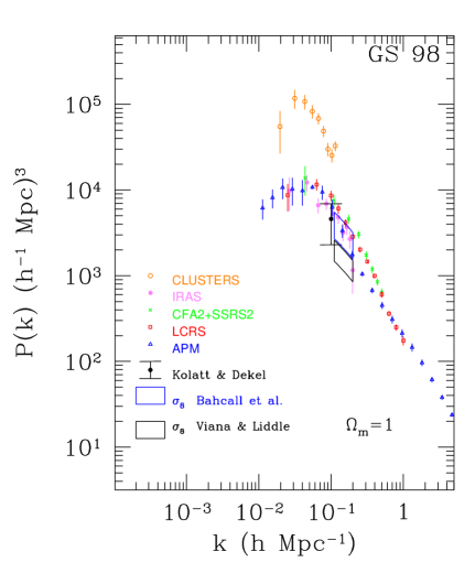
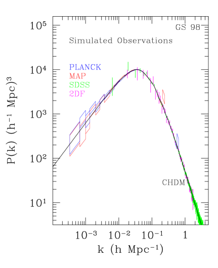
Figure 41: Compilation of large-scale structure observations, showing the power spectrum $P(k)$ as a function of wavenumber $k$. No corrections for bias, redshift distortions, or non-linear evolution have been made. Some of the redshift surveys have been rebinned to make the points nearly independent. The black box comes from measurements of $\sigma_{8}$ from present-day number abundances of rich clusters, and the black point with error bars is from peculiar velocities. The height shows the 68% confidence interval. $\Omega_{\rm M}=1$ is assumed. The right panel shows a simulation of high-precision future CMB and LSS observations. MAP (red boxes) and Planck (blue boxes) are simulated assuming that CHDM is the correct model. Green error bars show the accuracy of the Sloan Digital Sky Survey and magenta error bars are for the 2 Degree Field Survey. No corrections are made for redshift distortions or non-linear evolution. The simulated data are indistinguishable from the underlying CHDM model for a wide range of $k$. From Ref. [108].

The most ambitious and comprehensive galaxy survey currently in progress is without any doubt the Sloan Digital Sky Survey [112]. The aim of the project is first of all to observe photometrically the whole Northern Galactic Cap, 30^∘ away from the galactic plane (about $10^{4}$ deg²) in five bands, at limiting magnitudes from 20.8 to 23.3. The expectation is to detect around 50 million galaxies and around $10^{8}$ star-like sources. This has already led to the discovery of several high-redshift ($z>4$) quasars, including the highest-redshift quasar known, at $z=5.0$, see Ref. [112]. Using two fibre spectrographs carrying 320 fibres each, the spectroscopic part of the survey will then collect spectra from about $10^{6}$ galaxies with $r^{\prime}<18$ and $10^{5}$ AGNs with $r^{\prime}<19$. It will also select a sample of about $10^{5}$ red luminous galaxies with $r^{\prime}<19.5$, which will be observed spectroscopically, providing a nearly volume-limited sample of early-type galaxies with a median redshift of $z\simeq 0.5$, that will be extremely valuable to study the evolution of clustering. The data expected to arise from these new catalogs is so outstanding that already cosmologists are making simulations and predicting what will be the scientific outcome of these surveys, together with the future CMB anisotropy probes, for the determination of the cosmological parameters of the standard model of cosmology, see Figs. 41 and 42.

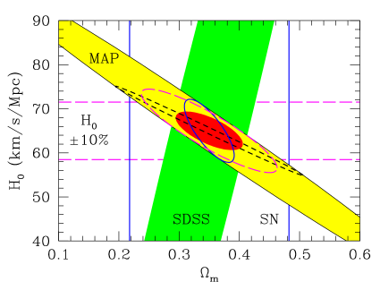
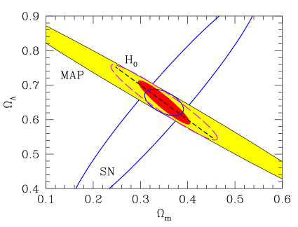
Figure 42: Constraint regions in the $\Omega_{\rm M}-H_{0}$ plane from various combinations of data sets. MAP data with polarization yields the ellipse from upper left to lower right; assuming the universe flat gives a smaller region (short-dashed line). SDSS ($k_{\rm max}=0.1h$ Mpc^-1) gives the vertical shaded region; combined with MAP gives the small filled ellipse. A projecton of future supernovae Ia results gives the solid vertical lines as bounds; combined with MAP gives the solid ellipse. A direct 10% measurement of $H_{0}$ gives the long-dashed lines and ellipse. All regions are 68% confidence. The fiducial model is the $\Omega_{\rm M}=0.35$ flat $\Lambda$CDM model. The right figure shows the same as before, but for constraints in the $\Omega_{\rm M}-\Omega_{\Lambda}$ plane. From Ref. [113].

As often happens in particle physics, not always are observations from a single experiment sufficient to isolate and determine the precise value of the parameters of the standard model. We mentioned in the previous Section that some of the cosmological parameters created similar effects in the temperature anisotropies of the microwave background. We say that these parameters are degenerate with respect to the observations. However, often one finds combinations of various experiments/observations which break the degeneracy, for example by depending on a different combination of parameters. This is precisely the case with the cosmological parameters, as measured by a combination of large-scale structure observations, microwave background anisotropies, Supernovae Ia observations and Hubble Space Telescope measurements, a feature named somewhat idiosyncratically as “cosmic complementarity”, see Ref. [113]. It is expected that in the near future we will be able to determine the parameters of the standard cosmological model with great precision from a combination of several different experiments, as shown in Fig. 42.

5 CONCLUSION

We have entered a new era in cosmology, were a host of high-precision measurements are already posing challenges to our understanding of the universe: the density of ordinary matter and the total amount of energy in the universe; the microwave background anisotropies on a fine-scale resolution; primordial deuterium abundance from quasar absorption lines; the acceleration parameter of the universe from high-redshift supernovae observations; the rate of expansion from gravitational lensing; large scale structure measurements of the distribution of galaxies and their evolution; and many more, which already put constraints on the parameter space of cosmological models, see Fig. 30. However, these are only the forerunners of the precision era in cosmology that will dominate the new millennium, and will make cosmology a phenomenological science.

It is important to bear in mind that all physical theories are approximations of reality that can fail if pushed too far. Physical science advances by incorporating earlier theories that are experimentally supported into larger, more encompassing frameworks. The standard Big Bang theory is supported by a wealth of evidence, nobody really doubts its validity anymore. However, in the last decade it has been incorporated into the larger picture of cosmological inflation, which has become the new standard cosmological model. All cosmological issues are now formulated in the context of the inflationary paradigm. It is the best explanation we have at the moment for the increasing set of cosmological observations.

In the next few years we will have an even larger set of high-quality observations that will test inflation and the cold dark matter paradigm of structure formation, and determine most of the 12 or more parameters of the standard cosmological model to a few percent accuracy (see table 1). It may seem that with such a large number of parameters one can fit almost anything. However, that is not the case when there is enough quantity and quality of data. An illustrative example is the standard model of particle physics, with around 21 parameters and a host of precise measurements from particle accelerators all over the world. This model is, nowadays, rigurously tested, and its parameters measured to a precision of better than 1% in some cases. It is clear that high-precision measurements will make the standard model of cosmology as robust as that of particle physics. In fact, it has been the technological advances of particle physics detectors that are mainly responsible for the burst of new data coming from cosmological observations. This is definitely a very healthy field, but there is still a lot to do. With the advent of better and larger precision experiments, cosmology is becoming a mature science, where speculation has given way to phenomenology.

There are still many unanswered fundamental questions in this emerging picture of cosmology. For instance, we still do not know the nature of the inflaton field, is it some new fundamental scalar field in the electroweak symmetry breaking sector, or is it just some effective description of a more fundamental high energy interaction? Hopefully, in the near future, experiments in particle physics might give us a clue to its nature. Inflation had its original inspiration in the Higgs field, the scalar field supposed to be responsible for the masses of elementary particles (quarks and leptons) and the breaking of the electroweak symmetry. Such a field has not been found yet, and its discovery at the future particle colliders would help understand one of the truly fundamental problems in physics, the origin of masses. If the experiments discover something completely new and unexpected, it would automatically affect inflation at a fundamental level.

One of the most difficult challenges that the new cosmology will have to face is understanding the origin of the cosmological constant, if indeed it is confirmed by independent sets of observations. Ever since Einstein introduced it as a way to counteract gravitational attraction, it has haunted cosmologists and particle physicists for decades. We still do not have a mechanism to explain its extraordinarily small value, 120 orders of magnitude below what is predicted by quantum physics. For several decades there has been the reasonable speculation that this fundamental problem may be related to the quantization of gravity. General relativity is a classical theory of space-time, and it has proved particularly difficult to construct a consistent quantum theory of gravity, since it involves fundamental issues like causality and the nature of space-time itself.

The value of the cosmological constant predicted by quantum physics is related to our lack of understanding of gravity at the microscopic level. However, its effect is dominant at the very largest scales of clusters or superclusters of galaxies, on truly macroscopic scales. This hints at what is known in quantum theory as an anomaly, a quantum phenomenon relating both ultraviolet (microscopic) and infrared (macroscopic) divergences. We can speculate that perhaps general relativity is not the correct description of gravity on the very largest scales. In fact, it is only in the last few billion years that the observable universe has become large enough that these global effects could be noticeable. In its infancy, the universe was much smaller than it is now, and, presumably, general relativity gave a correct description of its evolution, as confirmed by the successes of the standard Big Bang theory. As it expanded, larger and larger regions were encompassed, and, therefore, deviations from general relativity would slowly become important. It may well be that the recent determination of a cosmological constant from observations of supernovae at high redshifts is hinting at a fundamental misunderstanding of gravity on the very large scales.

If this were indeed the case, we should expect that the new generation of precise cosmological observations will not only affect our cosmological model of the universe but also a more fundamental description of nature.

References

- [1] A. Einstein, Sitz. Preuss. Akad. Wiss. Phys. 142 (1917) (§4); Ann. Phys. 69 (1922) 436.
- [2] A. Friedmann, Z. Phys. 10 (1922) 377.
- [3] E.P. Hubble, Publ. Nat. Acad. Sci. 15 (1929) 168.
- [4] G. Gamow, Phys. Rev. 70 (1946) 572; Phys. Rev. 74 (1948) 505.
- [5] A.A. Penzias and R.W. Wilson, Astrophys. J. 142 (1965) 419.
- [6] S. Weinberg, “Gravitation and Cosmology”, John Wiley & Sons (1972).
- [7] P.B. Pal, “Determination of cosmological parameters”, e-print Archive: hep-ph/9906447.
- [8] E.W. Kolb and M.S. Turner, “The Early Universe”, Addison Wesley (1990).
- [9] N. Arkani-Hamed, S. Dimopoulos and G. Dvali, Phys. Lett. B 429 (1998) 263, e-print Archive: hep-ph/9803315.
- [10] S. Burles, K.M. Nollett, J.N. Truran, M.S. Turner, Phys. Rev. Lett. 82 (1999) 4176, e-print Archive: astro-ph/9901157; S. Burles, K.M. Nollett, M.S. Turner, “Big-Bang Nucleosynthesis: Linking Inner Space and Outer Space”, e-print Archive: astro-ph/9903300.
- [11] K.A. Olive, G. Steigman and T. Walker, “Primordial Nucleosynthesis: Theory and Observations”, e-print Archive: astro-ph/9905320.
- [12] J.C. Mather et al., Astrophys. J. 420 (1994) 439; D.J. Fixen et al., Astrophys. J. 473 (1996) 576; J.C. Mather et al., Astrophys. J. 512 (1999) 511, e-print Archive: astro-ph/9810373.
- [13] R.H. Dicke, P.J.E. Peebles, P.G. Roll and D.T. Wilkinson, Astrophys. J. 142 (1965) 414.
- [14] G.F. Smoot, Astrophys. J. 396 (1992) L1; C.L. Bennett et al., Astrophys. J. 464 (1996) L1, e-print Archive: astro-ph/9601067.
- [15] P.J.E. Peebles, “Principles of Physical Cosmology”, Princeton U.P. (1993).
- [16] T. Padmanabhan, “Structure Formation in the Universe”, Cambridge U.P. (1993).
- [17] E.R. Harrison, Phys. Rev. D 1 (1970) 2726; Ya. B. Zel’dovich, Astron. Astrophys. 5 (1970) 84.
-
[18]
The IRAS Point Source Catalog Web page:
http://www-astro.physics.ox.ac.uk/~wjs/pscz.html - [19] L. Guzzo, “Large-scale structure at the turn of the millennium”, 19th Texas Symposium, Paris (1998), e-print Archive: astro-ph/9911115.
- [20] P.J. Steinhardt, in Particle and Nuclear Astrophysics and Cosmology in the Next Millennium, ed. by E.W. kolb and R. Peccei (World Scientific, Singapore, 1995).
- [21] W.L. Freedman, “Determination of cosmological parameters”, Nobel Symposium (1998), e-print Archive: hep-ph/9905222.
- [22] G.G. Raffelt, “Dark Matter: Motivation, Candidates and Searches”, European Summer School of High Energy Physics 1997. CERN Report pp. 235-278, e-print Archive: hep-ph/9712538.
- [23] S. Refsdael, Mon. Not. R. Astr. Soc. 128 (1964) 295; 132 (1966) 101.
- [24] R.D. Blandford and T. Kundić, “Gravitational Lensing and the Extragalactic Distance Scale”, e-print Archive: astro-ph/9611229.
- [25] N.A. Grogin and R. Narayan, Astrophys. J. 464 (1996) 92, e-print Archive: astro-ph/9512156.
- [26] M. Birkinshaw, Phys. Rep. 310 (1999) 97, e-print Archive: astro-ph/9808050.
-
[27]
The Chandra X-ray observatory Home Page:
http://chandra.harvard.edu/ - [28] S. Sakai et al., “The Hubble Space Telescope Key Project on the Extragalactic Distance Scale XXIV: The Calibration of Tully-Fisher Relations and the Value of the Hubble Constant”, e-print Archive: astro-ph/9909269.
- [29] F. Zwicky, Helv. Phys. Acata 6 (1933) 110.
- [30] M. Davis and J. Huchra, Astrophys. J. 254 (1982) 437; R.D. Kirshner et al., Astron. J. 88 (1983) 1285.
- [31] C.J. Copi and D.N. Schramm, Comm. Nucl. Part. Phys. 22 (1996) 1, e-print Archive: astro-ph/9504026.
- [32] K.C. Freeman, Astrophys. J. 160 (1970) 811.
- [33] K.G. Begeman, A.H. Broeils and R.H. Sanders, Mon. Not. R. Astr. Soc. 249 (1991) 523.
- [34] C.M. Baugh et al., “Ab initio galaxy formation”, e-print Archive: astro-ph/9907056; Astrophys. J. 498 (1998) 405; e-print Archive: astro-ph/9703111.
- [35] M. Fich and S. Tremaine, Annu. Rev. Astron. Astrophys. 29 (1991) 409.
- [36] A.D. Linde, J. García-Bellido and D. Wands, Phys. Rev. D 54 (1996) 4060. e-print Archive: astro-ph/9605094.
- [37] E. Roulet and S. Mollerach, Phys. Rep. 279 (1997) 68, e-print Archive: astro-ph/9603119.
- [38] The MACHO Collaboration, C. Alcock et al., “Microlensing results from 5.7 years of LMC observations”, e-print Archive: astro-ph/0001272.
- [39] B. Paczyński, Astrophys. J. 304 (1986) 1; Astrophys. J. Lett. 371 (1991) L63;
- [40] The MACHO Collaboration, C. Alcock et al., Nature 365 (1993) 621; MACHO Home Page at: http://wwwmacho.mcmaster.ca/
- [41] The EROS Collaboration, E. Aubourg et al., Nature 365 (1993) 623; EROS Home Page at: http://www.lal.in2p3.fr/recherche/eros/erosa.html
- [42] The AGAPE Collaboration, P. Baillon et al., A & A 277 (1993) 1; AGAPE Home Page at: http://cdfinfo.in2p3.fr/Experiences/AGAPE/frame-en.html
- [43] A. Dekel, Annu. Rev. Astron. Astrophys. 32 (1994) 371, e-print Archive: astro-ph/9401022.
- [44] R.G. Carlberg et al., Astrophys. J. 462 (1996) 32, e-print Archive: astro-ph/9509034.
- [45] A. Dekel, D. Burstein and S.D.M. White, “Measuring Omega”, in Critical Dialogues in Cosmology, ed. N. Turok, World Scientific (1997); e-print Archive: astro-ph/9611108.
- [46] C.L. Sarazin, Rev. Mod. Phys. 58 (1986) 1.
- [47] M. Bartelmann et al., Astron. & Astrophys. 330 (1998) 1, e-print Archive: astro-ph/9709229; M. Bartelmann and P. Schneider, “Weak Gravitational Lensing”, e-print Archive: astro-ph/9912508.
-
[48]
Hubble Space Telescope Web Page:
http://oposite.stsci.edu/pubinfo/subject.html - [49] N.A. Bahcall, J.P. Ostriker, S. Perlmutter and P.J. Steinhardt, Science 284 (1999) 1481, e-print Archive: astro-ph/9906463.
- [50] N.A. Bahcall and X. Fan, Proc. Nat. Acad. Sci. 95 (1998) 5956, e-print Archive: astro-ph/9804082; Astrophys. J. 504 (1998) 1, e-print Archive: astro-ph/9803277.
- [51] Particle Data Group Home Page, http://www.cern.ch/pdg/1999/lxxx.html
- [52] W. Hu, D.J. Eisenstein and M. Tegmark, Phys. Rev. Lett. 80 (1998) 5255, e-print Archive: astro-ph/9712057.
- [53] S.D. Tremaine and J.E. Gunn, Phys. Rev. Lett. 42 (1979) 407; J. Madsen, Phys. Rev. D 44 (1991) 999.
- [54] J. Primack, D. Seckel and B. Sadoulet, Ann. Rev. Nucl. Part. Sci. 38 (1988) 751; N.E. Booth, B. Cabrera and E. Fiorini, Ann. Rev. Nucl. Part. Sci. 46 (1996) 471.
- [55] S.M. Bilenky, “Neutrino masses, mixing and oscillations”, in these Proceedings; e-print Archive: hep-ph/0001311.
- [56] R. Bernabei et al., DAMA Collaboration, “Search for WIMP annual modulation signature: results from DAMA/NaI-3 and NaI-4, and the global combined analysis”, preprint INFN/AE-00/-01. DAMA Home Page, http://www.lngs.infn.it/lngs/htexts/dama/
- [57] J. Ellis, “Limits on Sparticle Dark Matter”, talk presented at COSMO 98, Asilomar, California, November 1998, e-print Archive: astro-ph/9903003.
- [58] For a recent review, see A. Morales, “Direct Detection of WIMP Dark Matter”, e-print Archive: astro-ph/9912554.
- [59] UK Dark Matter Collaboration (J.J. Quenby et al.), “Dark Matter Experiments at the UK Boulby mine”, at 26th International Cosmic Ray Conference (ICRC 99), in ‘Salt Lake City 1999, Cosmic ray’, Vol. 2, pp. 269–272. Home Page at http://hepwww.rl.ac.uk/ukdmc/
- [60] M. Bravin et al., Astropart. Phys. 12 (1999) 107; e-print Archive: hep-ex/9904005.
- [61] J.I. Collar et al., “First Dark Matter Limits from a Large-Mass, Low-Background Superheated Droplet Detector”, e-print Archive: astro-ph/0001511.
- [62] G. Jungman, M. Kamionkowski and K. Griest, Phys. Rep. 267 (1996) 195, e-print Archive: hep-ph/9506380.
- [63] The Alpha Matter Spectrometer Home Page: http://ams.cern.ch/AMS/
- [64] F. Halzen et al., Phys. Rep. 307 (1998) 243, e-print Archive: hep-ex/9804007.
- [65] S. Weinberg, Rev. Mod. Phys. 61 (1989) 1.
- [66] S.M. Carroll, W.H. Press and E.L. Turner, Ann. Rev. Astron. Astrophys. 30 (1992) 499.
- [67] J.P. Ostriker and P.J. Steinhardt, Nature 377 (1995) 600.
- [68] S. Perlmutter et al., The Supernova Cosmology Project, Bull. Am. Astron. Soc. 29 (1997) 1351, e-print Archive: astro-ph/9812473; Astrophys. J. 517 (1999) 565, e-print Archive: astro-ph/9812133.
- [69] A. Reiss et al., High Redshift Supernova Project, Astron. J. 116 (1998) 1009, e-print Archive: astro-ph/9805201.
- [70] C.S. Kochanek, Astrophys. J. 453 (1995) 545; Astrophys. J. 466 (1995) 638; E.E. Falco, C.S. Kochanek and J.A. Muñoz, Astrophys. J. 494 (1998) 47; e-print Archive: astro-ph/9707032.
- [71] P. de Bernardis et al., “Mapping the CMB Sky: The BOOMERANG experiment”, e-print Archive: astro-ph/9911461; A. Melchiorri et al., “A measurement of Omega from the North American test flight of BOOMERANG”, e-print Archive: astro-ph/9911445; P. D. Mauskopf et al.,“Measurement of a Peak in the Cosmic Microwave Background Power Spectrum from the North American test flight of BOOMERANG”, e-print Archive: astro-ph/9911444.
- [72] Microwave Anisotropy Probe Home Page: http://map.gsfc.nasa.gov/
- [73] Planck Home Page: http://astro.estec.esa.nl/Planck/
- [74] D.A. Vandenberg, M. Bolte and P.B. Stetson, Ann. Rev. Astron. Astrophys. 34 (1996) 461; e-print Archive: astro-ph/9605064.
- [75] L.M. Krauss, “The age of globular clusters”, e-print Archive: astro-ph/9907308.
- [76] B. Chaboyer, P. Demarque, P.J. Kernan and L.M. Krauss, Science 271 (1996) 957; Astrophys. J. 494 (1998) 96; e-print Archive: astro-ph/9706128.
- [77] C.H. Lineweaver, Science 284 (1999) 1503, e-print Archive: astro-ph/9911493.
- [78] J. García-Bellido, Phil. Trans. R. Soc. Lond. A 357 (1999) 3237, e-print Archive: astro-ph/9906497.
- [79] J. García-Bellido, “Inflationary Cosmology”, Vth Autumn School of Theoretical Physics, Santiago de Compostela (1997).
- [80] A. de Rújula, “Introduction to Cosmology”, CERN Summer Student Lecture Programme (1997).
- [81] A. Guth, Phys. Rev. D 23 (1981) 347.
- [82] A.D. Linde, Phys. Lett. 108B (1982) 389.
- [83] A. Albrecht and P.J. Steinhardt, Phys. Rev. Lett. 48 (1982) 1220.
- [84] For a personal historical account, see A. Guth, “The Inflationary Universe”, Perseus Books (1997).
- [85] A.D. Linde, “Particle Physics and Inflationary Cosmology”, Harwood Academic Press (1990).
- [86] A.R. Liddle and D.H. Lyth, Phys. Rep. 231 (1993) 1, e-print Archive: astro-ph/9303019.
- [87] J.M. Bardeen, Phys. Rev. D 22 (1980) 1882.
- [88] V.F. Mukhanov, H.A. Feldman and R.H. Brandenberger, Phys. Rep. 215 (1992) 203.
- [89] M. Abramowitz and I. Stegun, “Handbook of Mathematical Functions”, Dover (1972).
- [90] J. García-Bellido and D. Wands, Phys. Rev. D 53 (1996) 5437, e-print Archive: astro-ph/9511029.
- [91] D.H. Lyth and A. Riotto, Phys. Rep. 314 (1999) 1, e-print Archive: hep-ph/9807278.
- [92] D. Scott, J. Silk and M. White, Science 268 (1995) 829, e-print Archive: astro-ph/9505015; W. Hu, N. Sugiyama and J. Silk, Nature 386 (1997) 37, e-print Archive: astro-ph/9604166. E. Gawiser and J. Silk, “The Cosmic Microwave Background Radiation”, e-print Archive: astro-ph/0002044.
- [93] J. Silk, Nature 215 (1967) 1155;
-
[94]
M. Tegmark web page with latest experiments’ data:
http://www.hep.upenn.edu/~max/cmb/experiments.html - [95] R.K. Sachs and A.M. Wolfe, Astrophys. J. 147 (1967) 73.
- [96] E.R. Harrison, Rev. Mod. Phys. 39 (1967) 862; L.F. Abbott and R.K. Schaefer, Astrophys. J. 308 (1986) 546.
- [97] E.F. Bunn, A.R. Liddle and M. White, Phys. Rev. D 54 (1996) 5917, e-print Archive: astro-ph/9607038.
- [98] A.A. Starobinsky, Sov. Astron. Lett. 11 (1985) 133.
-
[99]
LIGO Home Page: http://www.ligo.caltech.edu/
VIRGO Home Page: http://www.virgo.infn.it/ - [100] M. Kamionkowski and A. Kosowsky, Ann. Rev. Nucl. Part. Sci. 49 (1999) 77, e-print Archive: astro-ph/9904108.
- [101] E. Torbet et al., Astrophys. J. 521 (1999) L79, e-print Archive: astro-ph/9905100; A. Miller et al., Astrophys. J. 524 (1999) L1, e-print Archive: astro-ph/990642.
- [102] L. Knox and L. Page, “Characterizing the Peak in the Cosmic Microwave Background Angular Power Spectrum”, e-print Archive: astro-ph/0002162.
-
[103]
CMBFAST code Home Page:
http://www.sns.ias.edu/~matiasz/CMBFAST/cmbfast.html - [104] L.A. Page, “Measuring the anisotropy in the CMB”, e-print Archive: astro-ph/9911199.
- [105] D. Scott, “New physics from the CMB”, e-print Archive: astro-ph/9911325.
- [106] A.R. Liddle and D.H. Lyth, “Cosmological Inflation and Large Scale Structure”, Cambridge University Press (2000).
- [107] J.R. Bond and G. Efstathiou, Astrophys. J. 285 (1984) L45.
- [108] E. Gawiser, J. Silk, Science 280 (1998) 1405, e-print Archive: astro-ph/9806197.
- [109] G. Efstathiou et al. (Eds.) “Large-scale structure in the universe”, Phil. Trans. R. Soc. Lond. A 357 (1999) 1-198.
- [110] B. Moore, Phil. Trans. R. Soc. Lond. A 357 (1999) 3259.
- [111] The 2 Degree Field Home Page: http://www.mso.anu.edu.au/2dFGRS/
- [112] The Sloan Digital Sky Survey Home Page: http://www.sdss.org/sdss.html
- [113] D.J. Eisenstein, W. Hu and M. Tegmark, Astrophys. J. 518 (1999) 2, e-print Archive: astro-ph/9807130.