The QCD Coupling Constant

Abstract

This paper presents a summary of the current status of determinations of the strong coupling constant $\alpha_{s}$. A detailed description of the definition, scale dependence and inherent theoretical ambiguities is given. The various physical processes that can be used to determine $\alpha_{s}$ are reviewed and attention is given to the uncertainties, both theoretical and experimental.

1 QCD AND ITS COUPLING

Quantum chromodynamics (QCD) is a gauge field theory that describes the strong interactions of quarks and gluons  [1]. All experimental results to date are consistent with QCD predictions to within the experimental and theoretical errors. In this review, we discuss the current status of the extraction of the strong interaction coupling constant $\alpha_{s}$ from the experimental data.

The QCD Lagrangian describing the interactions of quarks and gluons is

$$L=-{1\over 4}F_{\mu\nu}^{a}F^{a\mu\nu}+\sum_{k}\overline{\psi}_{k}\left(i\,\raise 0.6458pt\hbox{/}\mkern-13.5muD-m_{k}\right)\psi_{k},$$ (1)

where

$$F_{\mu\nu}^{a}=\partial_{\mu}A_{\nu}^{a}-\partial_{\nu}A_{\mu}^{a}+gf^{abc}A_{\mu}^{b}A_{\nu}^{c}$$ (2)

is the gluon field strength tensor,

$$D_{\mu}=\partial_{\mu}-igA_{\mu}^{a}T^{a}$$ (3)

is the gauge covariant derivative, and $T^{a}$ are the $SU(3)$ representation matrices normalized so that ${\rm tr\,}T^{a}T^{b}=\delta^{ab}/2$, and the sum on $k$ is over the six different flavors ($u,d,s,c,b,t$) of quarks. At the classical level, the QCD Lagrangian depends on the six quark masses $m_{k}$, and the strong interaction coupling constant $g$, or equivalently, the strong fine-structure constant $\alpha_{s}=g^{2}/4\pi$. The quantum theory contains an additional parameter, the $\theta$-angle, that violates CP. The experimental limit on this parameter is $\theta<10^{-9}$  [2], so we will set it to zero for the purposes of this article.

One can evaluate QCD scattering amplitudes in powers of $\alpha_{s}$ using a Feynman diagram expansion. As is typical in a quantum field theory, loop graphs are divergent and need to be treated using a renormalization scheme. The most commonly used scheme is modified minimal subtraction ($\overline{\rm MS}$)  [3], and we will use this scheme throughout. An important consequence of renormalization is that the parameters $\alpha_{s}$ and $m_{k}$ of the QCD Lagrangian depend in a calculable manner on the $\overline{\rm MS}$ subtraction-scale $\mu$. The $\mu$ dependence of $\alpha_{s}$ is described by the $\beta$-function,

$$\mu{d\alpha_{s}\over d\mu}=\beta\left(\alpha_{s}\left(\mu\right)\right).$$ (4)

In perturbation theory,

$$\beta\left(\alpha_{s}\right)=-{\beta_{0}}{\alpha_{s}^{2}\over 2\pi}-{\beta_{1}}{\alpha_{s}^{3}\over\left(2\pi\right)^{2}}-{\beta_{2}}{\alpha_{s}^{4}\over\left(2\pi\right)^{3}}-\ldots,$$ (5)

where (for $n_{f}$ flavors of quarks)

$$\beta_{0}=11-{2\over 3}n_{f},$$ (6)

$$\beta_{1}=51-{19\over 3}n_{f},$$ (7)

and the next two terms are also known  [5].

If $\alpha_{s}$ is small, the renormalization group equation Eq. (4) can be integrated using only the $\beta_{0}$ term to give

$${1\over\alpha_{s}(\mu_{1})}={1\over\alpha_{s}(\mu_{1})}+{\beta_{0}\over 2\pi}\ln{\mu_{1}\over\mu_{2}}.$$ (8)

Since $\beta_{0}>0$ for $n_{f}<16.5$, $\alpha_{s}(\mu)\to 0$ as $\mu\to\infty$. The vanishing of the QCD coupling for large values of $\mu$ is referred to as asymptotic freedom. One important consequence of asymptotic freedom, is that QCD processes at high energies can be reliably computed in a perturbation expansion in $\alpha_{s}$.

A measurable quantity, such as the total cross-section for $e^{+}e^{-}\to{\rm hadrons}$ at high energies can be computed as a function of the QCD coupling constant $\alpha_{s}(\mu)$ and the center of mass energy $E_{\rm CM}$,

$$\sigma\left(e^{+}e^{-}\to{\rm hadrons}\right)={1\over E_{\rm CM}^{2}}f\left(\alpha_{s}\left(\mu\right),\ln{E_{\rm CM}\over\mu}\right).$$ (9)

where $f$ is a dimensionless function of its arguments. The form of the cross-section given in Eq. (9) follows from dimensional analysis: $\sigma$ has dimensions of ${\rm energy}^{-2}$, and $\mu$ has dimensions of energy. In the $\overline{\rm MS}$ sscheme, any dependence on $\mu$ is logarithmic, so $f$ can only depend on $\ln E_{\rm CM}/\mu$. The cross section $\sigma\left(e^{+}e^{-}\to{\rm hadrons}\right)$ is a measurable quantity and cannot depend on the subtraction scale $\mu$, so the $\mu$ dependence on the right hand side of Eq. (9) must cancel,

$$\mu{d\over d\mu}f\left(\alpha_{s}\left(\mu\right),{E_{\rm CM}\over\mu}\right)=0,$$ (10)

and any value of $\mu$ can be used on the right hand side of Eq. (9). In practice, one can only compute the right hand side of Eq. (9) at some finite order in perturbation theory, and the approximate value of $f$ can depend on $\mu$ at higher order in perturbation theory. Typically, one finds that the perturbation expansion has terms of the form

$$\left[\alpha_{s}(\mu)\ln{E_{\rm CM}\over\mu}\right]^{n},$$ (11)

which are referred to as “leading logarithms.” Even if $\alpha_{s}(\mu)$ is small, the perturbation expansion can break down if $\ln{E_{\rm CM}/\mu}$ is large. For this reason, it is conventional to choose the subtraction scale of order the center of mass energy $E_{\rm CM}$. The exact choice of scale (for example, whether $\mu=2E_{\rm CM}$ or $E_{\rm CM}$ or $E_{\rm CM}/2$) is arbitrary, and differences in choice of scale are formally of higher order in $\alpha_{s}$. Many methods have been proposed to determine the optimum scale to use for a given calculation  [4]. The only way to determine the “best” scale at a given order is to compute the cross-section at next order. [Of course, in this case, one might as well use the more accurate formula to determine the cross-section.] The scale dependence of a given quantity can also be used to estimate the size of neglected higher order corrections. Scale dependence is a dominant source of error in many of the quantities that will be used to determine $\alpha_{s}$.

Perturbation theory is valid if one chooses $\mu$ to be of order $E_{\rm CM}$, so that the expansion parameter is $\alpha_{s}(E_{\rm CM})$, with no large logarithms. This shows that at high-energies, the coupling constant is small because of asymptotic freedom, and QCD cross-sections are approximately those of free quarks and gluons. At low, energies, non-perturbative effects become important.

The value of $\alpha_{s}$ is determined by computing a quantity in terms of $\alpha_{s}$, and comparing with its measured value. One might think that it is better to use high-energy processes to determine $\alpha_{s}$, since perturbation theory is more reliable. This is not necessarily the case. High energy processes can be computed more reliably precisely because they do not depend very much on $\alpha_{s}$. This means that errors in the experimental measurement or theoretical calculation get amplified when they are converted to an error on $\alpha_{s}$. We will see in this article that low-energy extractions of $\alpha_{s}$ have comparable errors to those at high energy.

In addition to scale dependence, the coupling constant $\alpha_{s}$ is also subtraction scheme dependent. The scheme dependence of the coupling constant is compensated for by the scheme dependence in the functional form for a measurable quantity, so that the value of an observable is scheme independent. The $\overline{\rm MS}$ scheme will be used in this article, but there is still some residual scheme dependence we need to consider. In the $\overline{\rm MS}$ scheme, heavy quarks do not decouple in loop graphs at low-energy. For example, the $\beta$-function coefficient $\beta_{0}=11-2n_{f}/3$, where $n_{f}$ is the number of quark flavors. This expression is true for all energies, irrespective of the mass of the quark. One might expect that at energies much smaller than the mass $m_{Q}$ of a heavy quark, the quark does not contribute to the $\beta$-function. This cannot happen in the $\overline{\rm MS}$ scheme, since $\overline{\rm MS}$ is a mass-independent subtraction scheme, which results in a mass-independent $\beta$-function. What happens is that there are large logarithms of the form $\ln m_{Q}/\mu$ that compensate for the “incorrect” $\beta$-function at low-energies. In practice, one deals with this problem using an effective field theory. At energies smaller than $m_{Q}$, one switches from a QCD Lagrangian with $n_{f}$ flavors to a QCD Lagrangian with $n_{f}-1$ flavors by integrating out the heavy quark flavor. The effect of the heavy quark is taken into account by higher dimension operators in the QCD Lagrangian, and by shifts in the parameters $\alpha_{s}$ and $m_{k}$. Thus it is necessary to specify the effective theory when quoting the value of $\alpha_{s}$. We will use the notation $\alpha_{s}^{(n_{f})}$ to denote the value of $\alpha_{s}$ in the $n_{f}$ flavor theory. One can compute the relation between $\alpha_{s}^{(n_{f})}$ and $\alpha_{s}^{(n_{f}-1)}$ at the scale $\mu=m_{Q}$ of the heavy quark. This relation is known to three loops  [6],

$$\alpha_{s}^{(n_{f}-1)}\left(m_{Q}\right) = \alpha_{s}^{(n_{f})}\left(m_{Q}\right)\left[1+0.1528\left({\alpha_{s}^{(n_{f})}\left(m_{Q}\right)\over\pi}\right)^{2}\right.$$ (12)

$$\left.+(0.9721-0.0847n_{f})\left({\alpha_{s}^{(n_{f})}\left(m_{Q}\right)\over\pi}\right)^{3}+\ldots\right].$$

When quoting the value of $\alpha_{s}(\mu)$, it is also necessary to specify the number of flavors in the effective theory. In most of the $\alpha_{s}$ determinations we consider, the appropriate effective theory to use is one with $n_{f}=5$, and $\alpha_{s}$ will refer to $\alpha_{s}^{(5)}$ unless otherwise specified.

Classical QCD is a scale invariant theory, but this scale invariance is broken at the quantum level. The quantum theory has a dimensionful parameter $\Lambda$ that characterizes the scale of the strong interactions. The $\Lambda$ parameter is determined in terms of $\alpha_{s}(\mu)$. The solution of the renormalization group equation Eq. (4) including the first three terms in the $\beta$-function is

$$\alpha_{s}(\mu) = {4\pi\over\beta_{0}\ln\left(\mu^{2}/\Lambda^{2}\right)}\left[1-{2\beta_{1}\over\beta_{0}^{2}}{\ln\left[\ln\left(\mu^{2}/\Lambda^{2}\right)\right]\over\ln\left(\mu^{2}/\Lambda^{2}\right)}\right.$$ (13)

$$\left.+{4\beta_{1}^{2}\over\beta_{0}^{4}\ln^{2}\left(\mu^{2}/\Lambda^{2}\right)}\left(\left(\ln\left[\ln\left(\mu^{2}/\Lambda^{2}\right)\right]-{1\over 2}\right)^{2}+{\beta_{2}\beta_{0}\over\beta_{1}^{2}}-{5\over 4}\right)\right].$$

This equation can be used to determine $\Lambda$ if $\alpha_{s}$ is known at some scale $\mu$. The value of $\Lambda$ depends on the number of terms retained in Eq. (13). The expansion parameter in Eq. (13) is

$${\ln\left[\ln\left(\mu^{2}/\Lambda^{2}\right)\right]\over\ln\left(\mu^{2}/\Lambda^{2}\right)},$$ (14)

which is small as long as $\mu\gg\Lambda$. In QCD, $\Lambda$ is of order 200  MeV. The last term in Eq. (13) is often dropped in the definition of $\Lambda$. For a fixed value of $\alpha_{s}(M_{Z})$, the shift in $\Lambda$ is approximately 15 MeV if the last term in Eq. (13) is dropped.

The QCD $\beta$-function depends on $n_{f}$, and so changes across quark thresholds. This in turn implies that $\Lambda$ changes across quark thresholds, so that $\Lambda^{(n_{f})}$ is the value of $\Lambda$ with $n_{f}$ dynamical quark flavors. The matching conditions for $\Lambda^{(n_{f})}\to\Lambda^{(n_{f}-1)}$ can be computed using the matching condition Eq. (12) for $\alpha_{s}$. The differences between $\Lambda^{(3)}$, $\Lambda^{(4)}$, and $\Lambda^{(5)}$ are numerically very significant.

In addition to the perturbative effects discussed so far, non-perturbative effects play an important role in strong interaction processes. The size of non-perturbative effects is governed by the ratio of the strong interaction scale $\Lambda$ to the typical energy $E_{\rm CM}$ of a given process. In many cases, non-perturbative effects are estimated using a model analysis, or by a phenomenological fit to the experimental data. A few processes can be analyzed rigorously using the operator product expansion (OPE) [7]; in this case, one can calculate the size of non-perturbative effects in terms of matrix elements of gauge invariant local operators. Two classic examples of this type are deep inelastic scattering, and the total cross-section for $e^{+}e^{-}\to{\rm hadrons}$.

It is convenient to calculate $R(s)$, the ratio of the total cross-sections for $e^{+}e^{-}\to{\rm hadrons}$ and $e^{+}e^{-}\to\mu^{+}\mu^{-}$ at center of mass-energy $E_{\rm CM}=\sqrt{s}$. One can show that

$$R(s)=f_{0}\left(\alpha_{s}(s)\right)+f_{1}\left(\alpha_{s}(s)\right){\left\langle{{F_{\mu\nu}F^{\mu\nu}}}\right\rangle\over s^{2}}+\ldots,$$ (15)

where the first non-perturbative correction depends on the vacuum expectation value of the square of the gluon field-strength tensor. By dimensional analysis, this quantity is of order $\Lambda^{4}$, so the non-perturbative corrections are of order $\Lambda^{4}/s^{2}$. The existence of an OPE provides some crucial information on the size of non-perturbative corrections. For $R(s)$, we know that the corrections vanish at least as fast as $\Lambda^{4}/s^{2}$ for large values of $s$, because $F_{\mu\nu}F^{\mu\nu}$ is the lowest dimension operator that can contribute in the OPE. Similarly, it is known in deep inelastic scattering that the first non-perturbative corrections arise from twist-four operators, and are of order $\Lambda^{2}/Q^{2}$, where $Q$ is the momentum transfer. One can estimate the size of non-perturbative corrections for processes with an OPE, by estimating the value of operator matrix elements. In some cases, one is fortunate enough that the relevant matrix element can actually be determined from some other measurement, or computed from first principles. The size of non-perturbative corrections is much less certain if the process does not have an OPE. Non-perturbative effects can fall off like a fractional power of $\Lambda/s$, or could have some more complicated dependence on $s$. Typically, one uses some model estimate of the non-perturbative corrections.

Perturbative and non-perturbative corrections to scattering cross-sections are interrelated, because the QCD perturbation series is an asymptotic expansion, rather than a convergent expansion. A dimensionless quantity $f(\alpha_{s})$ has an expansion of the form

$$f(\alpha_{s})=c_{0}+c_{1}\alpha_{s}+c_{2}\alpha_{s}^{2}+\ldots.$$ (16)

Typically, the coefficients $c_{n}$ grow as $n!$, so that the series has zero radius of convergence. The large-order behavior of the perturbation series can be computed in certain limiting cases  [8, 9, 10, 11, 12, 13]. If one studies QCD in the limit of a large number of flavors, $n_{f}\to\infty$, with $\alpha_{s}n_{f}$ fixed, one can sum all terms of the form $(\alpha_{s}n_{f})^{n}$. This is sometimes referred to as the “bubble chain” approximation, because the graphs one sums are of the type show in Fig. 1.

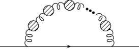
Figure 1: Graphs that contribute to the propagator correction in the bubble chain approximation.

QCD is not asymptotically free as $n_{f}\to\infty$. Nevertheless, one can try and apply the bubble chain results to QCD. The bubble chain graphs contribute to the QCD $\beta$-function. In the large $n_{f}$ limit, the coefficient $\beta_{0}=11-2/3n_{f}\to-2/3n_{f}$. One therefore computes the bubble chain sum, makes the replacement $n_{f}\to-3\beta_{0}/2$, and uses the resultant expression for QCD with $\beta_{0}>0$. This seemingly unjustified procedure has provided some useful insights into the nature of the QCD perturbation series. A detailed discussion of this method is beyond the scope of the present article. It is typically found that the coefficients $c_{n}$ in the perturbation expansion have a factorial divergence in the bubble chain approximation. One can try and sum a series of this type using a Borel transformation. One defines the Borel transform of $f$ by

$$f_{B}(t)=c_{0}\delta(t)+c_{1}+c_{2}t+\ldots+{c_{n+1}\over n!}t^{n}+\ldots.$$ (17)

Then the original function can be obtained by the inverse Borel transform,

$$f(\alpha_{s})=\int_{0}^{\infty}dt\ f_{B}(t)e^{-t/\alpha_{s}}.$$ (18)

Suppose the coefficients of $f(\alpha_{s})$ have the form

$$c_{n+1}=a^{n}n!,\ \ n>0.$$ (19)

Then

$$f_{B}(t)=c_{0}\delta(t)+\sum_{n=0}^{\infty}a^{n}t^{n}=c_{0}\delta(t)+{1\over 1-at},$$ (20)

and the inverse Borel transform gives

$$f(\alpha_{s})=c_{0}+\int_{0}^{\infty}dt\ e^{-t/\alpha_{s}}{1\over 1-at}.$$ (21)

The behavior of the integral is governed by the singularities in the complex $t$ plane, which are referred to as renormalons. If $a<0$, the integral is well-defined, since the singularity at $t=1/a$ is not along the path of integration. If $a>0$, the singularity is along the contour of integration. One can regulate the integral by deforming the contour around the singularity. The integral depends on the precise prescription used. The prescription dependence is related to the pole at $t=1/a$, which gives a contribution to the integral of the form

$$\exp\left[-{1\over a\alpha_{s}}\right]=\exp\left[{-\beta_{0}\ln(\mu/\Lambda)\over 2\pi a}\right]=\left({\Lambda\over\mu}\right)^{\beta_{0}/2\pi a}.$$ (22)

The value of $\mu$ is chosen to be the typical energy in the process, such as the momentum transfer $Q$ for deep inelastic scattering. The perturbative series then has the same structure as a typical non-perturbative correction, a power law correction of the form

$$\left({\Lambda^{2}\over Q^{2}}\right)^{u_{0}}$$ (23)

where $u_{0}=\beta_{0}/(4\pi a)$ is the renormalon singularity in the variable $u=\beta_{0}t/(4\pi)$. [It is conventional to refer to the location of the renormalon singularity in $u$ rather than in $t$.] Contributions of the form Eq. (23) are called renormalon ambiguities, since their value depends on the way in which one performs the inverse Borel transform.

Renormalon ambiguities have the same structure as non-perturbative corrections. It has been suggested in the literature  [13] that renormalons can be used as a guide to the size of non-perturbative corrections. There is one non-trivial check to this idea. A renormalon singularity at $u_{0}$ corresponds to a non-perturbative ambiguity of the form Eq. (23). In processes that have an OPE, all non-perturbative effects should be given by the matrix elements of gauge invariant local operators. To every renormalon ambiguity in the perturbation expansion, there should be a corresponding ambiguity in the operator matrix element, such that the sum is well-defined  [10]. This can only happen provided that there is a gauge invariant local operator corresponding to every renormalon singularity. For example, the first gauge invariant operator corrections to deep inelastic scattering are of the form $\Lambda^{2}/Q^{2}$, and it is known that the first renormalon ambiguity is at $u=1$. Similarly, for $R$, the first non-perturbative corrections are of the form $\Lambda^{4}/Q^{4}$, and the first renormalon ambiguity is at $u=2$. The matching between renormalon singularities and the OPE occurs in all examples that have been computed so far. For this reason, renormalon singularities have also been taken as an indication of the size of non-perturbative effects in processes without an OPE. Non-perturbative effects are expected to fall off faster if the renormalons are at larger values of $u$.

Infrared sensitivity is also used to estimate the size of non-perturbative corrections to a measurable quantity  [15]. One computes the quantity in the presence of an infrared cutoff momentum $\lambda$. For example, one can imagine working in a box of size $1/\lambda$, or using a gluon mass of order $\lambda$. Cross-sections can have infrared divergences of the form $\ln\lambda$. If one computes measurable cross-sections for color singlet states to scatter into color singlet states, one finds that the $\ln\lambda$ terms cancel, and the cross-section is infrared finite, a result known as the KLN  [14] theorem. It is important to include finite detector resolution to get a finite cross-section, as for QED. For example, the Bhabha scattering cross-section for $e^{+}e^{-}\to e^{+}e^{-}$ has an infrared divergence at one-loop order. However, it is impossible to distinguish $e^{+}e^{-}\to e^{+}e^{-}$ from $e^{+}e^{-}\to e^{+}e^{-}\gamma$ if the photon energy $E_{\gamma}$ is smaller than the detector resolution $\delta$. The measurable quantity is the sum of the $e^{+}e^{-}\to e^{+}e^{-}$ cross-section and the $e^{+}e^{-}\to e^{+}e^{-}\gamma$ cross-section for $E_{\gamma}<\delta$, which is free of infrared singularities. While the $\ln\lambda$ term must cancel, terms of order $\lambda$, $\lambda^{2}\ln\lambda$, etc. which vanish as $\lambda\to 0$ need not cancel. The first non-vanishing term is an indication of the infrared-sensitivity of a given quantity. In QCD, one can imagine that the scale $\lambda$ represents the confinement scale $\Lambda$. A process that is infrared sensitive at order $\lambda^{n}$ would then be expected to have non-perturbative corrections of order $\Lambda^{n}/Q^{n}$, where $Q$ is the typical momentum transfer. In a few cases, one can analyze the problem using renormalon methods, and by using the criterion of infrared sensitivity. It is found in these cases that both methods give the same estimate for the size of non-perturbative corrections.

2 $\alpha_{s}$ FROM $Z$ DECAYS AND $e^{+}e^{-}$ TOTAL RATES

The total cross section for $e^{+}e^{-}\to\hbox{hadrons}$ is obtained (at low values of $\sqrt{s}$) by multiplying the muon-pair cross section by the factor $R$. At lowest order in QCD perturbation theory $R=R^{0}=3\Sigma_{q}e_{q}^{2}$ where $e_{q}$ is the electric charge of the quark of flavor $q$. The higher-order QCD corrections to this are known, and the results can be expressed in terms of the factor:

$$R=R^{(0)}\left[1+\frac{\alpha_{s}}{\pi}+C_{2}\left(\frac{\alpha_{s}}{\pi}\right)^{2}+C_{3}\left(\frac{\alpha_{s}}{\pi}\right)^{3}+\;\cdots\;\;\right]$$ (24)

where $C_{2}=1.411$ and $C_{3}=-12.8$ [16].

This result is only correct in the zero-quark-mass limit. The ${\cal O}(\alpha_{s}$) corrections are also known for massive quarks [17]. The principal advantages of determining $\alpha_{s}$ from $R$ in $e^{+}e^{-}$ annihilation are that the measurement is inclusive, that there is no dependence on the details of the hadronic final state and that non-perturbative corrections are suppressed by $1/s^{2}$.

A measurement by CLEO  [18] at $\sqrt{s}=10.52$ GeV yields $\alpha_{s}(10.52\hbox{ GeV})=0.20\pm 0.01\pm 0.06$ which corresponds to $\alpha_{s}(M_{Z})=0.13\pm 0.005\pm 0.03.$ A comparison of the theoretical prediction of Eqn. 24 (corrected for the $b$-quark mass), with all the available data at values of $\sqrt{s}$ between 20 and 65 GeV, gives [19] $\alpha_{s}(35\hbox{ GeV})=0.146\pm 0.030.$ It should be noted that the size of the order $\alpha_{s}^{3}$ term is of order 40% of that of the order $\alpha_{s}^{2}$ and 3% of the order $\alpha_{s}$. If the order $\alpha_{s}^{3}$ term is not included, the extracted value decreases to $\alpha_{s}~{}(35\hbox{ GeV})=0.142\pm 0.03$, a difference smaller than the experimental error.

Measurements of the ratio of the hadronic to leptonic width of the $Z$ at LEP and SLC, $\Gamma_{h}/\Gamma_{\mu}$ probe the same quantity as $R$. Using the average of $\Gamma_{h}/\Gamma_{\mu}=20.783\pm 0.029$ gives $\alpha_{s}(M_{Z})=0.123\pm 0.004$ [20]. The prediction depends upon the couplings of the quarks and leptons to the $Z$. The precision is such that higher order electroweak corrections to these couplings must be included. There are theoretical errors arising from the values of top-quark and Higgs masses which enter in these radiative corrections. Hence, while this method has small theoretical uncertainties from QCD itself, it relies sensitively on the electroweak couplings of the $Z$ to quarks [21] and on the ability of the Standard Model of electroweak interactions to predict these correctly. The presence of new physics which changes these couplings via electroweak radiative corrections would invalidate the extracted value of $\alpha_{s}(M_{Z})$. Since the Standard Model fits the measured $Z$ properties well, this concern is ameliorated and more precise value of $\alpha_{s}$ can be obtained by using a global fit to the many precisely measured properties of the $Z$ boson and the measured $W$ and top masses. This gives  [22]

$$\alpha_{s}(M_{Z})=0.1192\pm 0.0028$$

This error is larger than the shift in the value of $\alpha_{s}(M_{Z})$ ($\sim 0.002$) that would result if the order $\alpha_{s}(M_{Z})^{3}$ term were omitted and hence one can conclude that it is very unlikely that the uncertainty due to the unknown $\alpha_{s}(M_{Z})^{4}$ terms will dominate over the experimental uncertainty.

3 DETERMINATION OF $\alpha_{s}$ FROM DEEP INELASTIC SCATTERING

The original and still one of the most powerful quantitative tests of perturbative QCD is the breaking of Bjorken scaling in deep-inelastic lepton-hadron scattering. Consider the case of electron-proton scattering ($ep\to eX$), where the cross-section can be written as

$$\frac{d\sigma}{dxdy}=\frac{4\pi\alpha_{em}^{2}s}{Q^{4}}\left[\frac{1+(1-y)^{2}}{2}2xF_{1}(x,Q^{2})+(1-y)(F_{2}(x,Q^{2})-2xF_{1}(x,Q^{2}))\right]$$ (25)

The variables are defined as follows (see Figure 2): $q$ is the momentum of the exchanged photon, $P$ is the momentum of the target proton, $k$ is that of the incoming electron, and

$$Q^{2} =-q^{2}$$

$$\nu =\frac{q\cdot P}{m_{p}}$$

$$x =\frac{Q^{2}}{2m_{p}\nu}$$

$$y =\frac{q\cdot p}{k\cdot p}$$

$$s =2p\cdot k+m_{p}^{2}$$

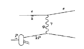
Figure 2: Figure showing the kinematics of deep inelastic scattering $ep\to eX$

For charged current scattering, which proceeds via the exchange of a virtual $W$ boson between the lepton and target nucleus, there is an additional parity violating structure function $F_{3}$

$$\begin{array}[]{ll}\displaystyle\frac{d\sigma^{\nu N}}{dxdy}=&\displaystyle\frac{G_{F}^{2}M_{W}^{4}s}{2\pi(Q^{2}+M_{W}^{2})^{2}}(xy^{2}F_{1}^{\nu N}(x,Q^{2})\cr&\displaystyle+(1-y-x^{2}y^{2}M^{2}/Q^{2})F_{2}^{\nu N}(x,Q^{2})\cr&\displaystyle-\frac{1}{2}x((1-y)^{2}-1)F_{3}^{\nu N}(x,Q^{2}))\end{array}$$ (27)

For $\overline{\nu}N$ scattering the sign of the last ($xF_{3}$) term is reversed.

In the leading-logarithm approximation, the measured structure functions $F_{i}(x,Q^{2}$) are related to the quark distribution functions $q_{i}(x,Q^{2})$ according to the naive parton model, for example

$$F_{2}(x,Q^{2})=\sum_{i}e_{i}^{2}q_{i}(x,Q^{2})$$ (28)

Here $q_{i}(x,Q^{2})$ is the probability for a parton of type $i$ to carry a fraction $x$ of the nucleon’s momentum. The $Q^{2}$ dependence of the parton distribution functions is predicted by perturbative QCD, hence a measurement of the $Q^{2}$ dependence (“scaling violation”) can by used to measure $\alpha_{s}$. In describing the way in which scaling is broken in QCD, it is convenient to define nonsinglet and singlet quark distributions:

$$F^{NS}=q_{i}-q_{j}\qquad\qquad F^{S}=\sum_{i}(q_{i}+\overline{q}_{i})$$

The nonsinglet structure functions have nonzero values of flavor quantum numbers such as isospin or baryon number. The variation with $Q^{2}$ of these is described by the so-called DGLAP equations [23] [24]:

$$\begin{array}[]{ll}Q^{2}\;\frac{\partial F^{NS}}{\partial Q^{2}}&=\frac{\alpha_{s}(|Q|)}{2\pi}P^{qq}\ast F^{NS}\\ \cr Q^{2}\;\frac{\partial}{\partial Q^{2}}\left({F^{S}\atop G}\right)&=\frac{\alpha_{s}(|Q|)}{2\pi}\left({P^{qq}\phantom{{}_{q}}\atop P^{gq\phantom{{}^{Y}}}}\;{2n_{f}P^{qg}\atop P^{{gg}\phantom{{}^{Y}}}}\right)\ast\left({F^{S}\atop G}\right)\end{array}$$

where $\ast$ denotes a convolution integral:

$$f\ast g=\int_{x}^{1}\frac{dy}{y}\;f(y)\;g\left(\frac{x}{y}\right)$$

The leading-order Altarelli-Parisi [24] splitting functions are

$$\begin{array}[]{ll}P^{qq}&=\frac{4}{3}\left[\frac{1+x^{2}}{(1-x)_{+}}\right]+2\delta(1-x)\cr P^{qg}&=\frac{1}{2}\left[x^{2}+(1-x)^{2}\right]\cr P^{gq}&=\frac{4}{3}\left[\frac{1+(1-x)^{2}}{x}\right]\cr P^{gg}&=6\left[\frac{1-x}{x}+x(1-x)+\frac{x}{(1-x)_{+}}+\frac{11}{12}\delta(1-x)\right]\cr&\qquad-\frac{n_{f}}{3}\delta(1-x)\end{array}$$

Here the gluon distribution $G(x,Q^{2})$ has been introduced and $1/(1-x)_{+}$ means

$$\int_{0}^{1}dx\frac{f(x)}{(1-x)_{+}}=\int_{0}^{1}dx\;\frac{f(x)-f(1)}{(1-x)}$$

Measurement of the structure functions over a large range of $x$ and $Q^{2}$ allows both $\alpha_{s}$ and the parton distributions to be determined. Notice that $\alpha_{s}$ and the gluon distribution can only be obtained by measuring the $Q^{2}$ dependence. The precision of contemporary experimental data demands that higher-order corrections also be included [25]. The above results are for massless quarks. Algorithms exist for the inclusion of nonzero quark masses [26]. These are particularly important for neutrino scattering near the charm threshold. At low $Q^{2}$ values, there are also important “higher-twist” (HT) contributions of the form:

$$F_{i}(x,Q^{2})=F_{i}^{(LT)}\;(x,Q^{2})+\frac{F_{i}^{(HT)}(x,Q^{2})}{Q^{2}}+\;\cdots$$

Leading twist (LT) terms are those whose behavior can be predicted using the parton model, and are related to the parton distribution functions. Higher-twist corrections depend on matrix elements of higher dimension operators. These corrections are numerically important only for $Q^{2}\!<\!{\cal O}$(few GeV²) except for $x$ very close to 1. At very large values of $x$ corrections proportional to $\log(1-x)$ can become important [27].

From Eqn. LABEL:AltarelliParisi;a, it is clear that a nonsinglet structure function offers in principle the most precise test of the theory, since the $Q^{2}$ evolution is independent of the unmeasured gluon distribution. The CCFR collaboration fit to the Gross-Llewellyn Smith sum rule [28] which is known to order $\alpha_{s}^{3}$ [29] [30] (Estimates of the order $\alpha_{s}^{4}$ term are available [31])

$$\begin{array}[]{ll}&\int_{0}^{1}dx\left\{F_{3}^{\overline{\nu}p}(x,Q^{2})+F_{3}^{{\nu}p}(x,Q^{2})\right\}=\cr&~{}~{}~{}~{}3\left[1-\frac{\alpha_{s}}{\pi}(1+3.58\frac{\alpha_{s}}{\pi}+19.0(\frac{\alpha_{s}}{\pi})^{2})\right]-\Delta{HT}\end{array}$$

where the higher-twist contribution $\Delta{HT}$ is estimated to be $(0.09\pm 0.045)/Q^{2}$ in  [29] [32] and to be somewhat smaller by  [33]. The CCFR collaboration [34], combines their data with that from other experiments  [35] and gives $\alpha_{s}~{}(\sqrt{3}~{}\hbox{GeV})=0.28\pm 0.035~{}(\hbox{expt.})\pm 0.05~{}(\hbox{sys})^{+0.035}_{-0.03}~{}(\hbox{theory})$. The error from higher-twist terms (assumed to be $\Delta{HT}=0.05\pm 0.05$) dominates the theoretical error. If the higher twist result of  [33] is used, the central value increases to 0.31 in agreement with the fit of  [36]. This value extrapolates to $\alpha_{s}~{}(M_{Z})=0.118\pm 0.011$.

Measurements involving singlet-dominated structure functions, such as $F_{2}$, result in correlated measurements of $\alpha_{s}$ and the gluon structure function. A full next to leading order fit combining data from SLAC [37], BCDMS [38], E665 [39] and HERA [40]has been performed  [41]. These authors extend the analysis to next to next to leading order (NNLO). In this case the full theoretical calculation is not available as not all the three-loop anomalous dimensions are known; their analysis uses moments of structure functions and is restricted to those moments where the full calculation is available  [25, 42, 36]. The NNLO result is $\alpha_{s}~{}(M_{Z})=0.1172\pm 0.0017~{}(\hbox{expt.})\pm 0.0017~{}(\hbox{sys})$. Here the first error is a combination of statistical and systematic experimental errors, and the second error is due to the uncertainties, quark masses, higher twist and target mass corrections, and errors from the gluon distribution. If only a next to leading order fit is performed then the value decreases to $\alpha_{s}~{}(M_{Z})=0.116$ indicating that the theoretical results are stable. No error is included from the choice of $\mu$; $\mu=Q$ is assumed. We use a total error of $\pm 0.0045$ to take into account an estimate of the scale uncertainty. This result is consistent with earlier determinations  [43],  [44], and  [45].

The spin-dependent structure functions, measured in polarized lepton nucleon scattering, can also be used to determine $\alpha_{s}$. The spin structure functions $G_{1}$ and $G_{2}$ are defined in terms of the asymmetry in polarized lepton nucleon scattering

$$a(x,y)=\frac{d\sigma^{eN}_{p}}{dxdy}-\frac{d\sigma^{eN}_{ap}}{dxdy}$$ (29)

where the subscript $p$ ($ap$) refers to the state where the nucleon spin is parallel (anti-parallel) to its direction of motion in the center of mass frame of the lepton-nucleon system. In both cases the lepton has its spin aligned along its direction of motion.

$$\begin{array}[]{ll}a(x,y)=&\displaystyle\frac{8\pi\alpha_{em}^{2}y}{MQ^{2}}((1-2/y^{2}+2x^{2}y^{2}M^{2}/Q^{2})G_{1}(x,Q^{2})\\ &+4x^{2}M^{2}G_{2}(x,Q^{2})/Q^{2})\end{array}$$ (30)

The $Q^{2}$ evolution of the spin structure functions $G_{1}(x,Q^{2})$ and $G_{2}(x,Q^{2})$ is similar to that of the unpolarized ones and is known at next to leading order  [51].Here the values of $Q^{2}\sim 2.5\hbox{ GeV}^{2}$ are small particularly for the E143 data  [46] and higher-twist corrections are important. A fit [47] using the measured spin dependent structure functions measured by themselves and by other experiments  [48] [46] gives $\alpha_{s}(M_{Z})=0.121\pm 0.002(\hbox{expt.})\pm 0.006(\hbox{theory and syst.})$. Data from HERMES  [49] are not included in this fit; they are consistent with the older data.

$\alpha_{s}$ can also be determined from the Bjorken sum rule [50].

$$S_{{\rm Bj}}=\int_{0}^{1}dx\left(G_{1}^{p}-G_{1}^{n}\right)=\frac{1}{6}a_{3}$$ (31)

At lowest order in QCD $a_{3}=g_{A}=\frac{G_{V}}{G_{A}}=1.2573\pm 0.0028$. A fit gives  [52] $\alpha_{s}(M_{Z})=0.118^{+0.010}_{-0.024}$; a significant contribution to the error being due to the extrapolation into the (unmeasured) small $x$ region. Theoretically, the sum rule is preferable as the perturbative QCD result is known to higher order, and these terms are important at the low $Q^{2}$ involved. It has been shown that the theoretical errors associated with the choice of scale are considerably reduced by the use of Pade approximants [53] which results in $\alpha_{s}(1.7~{}\hbox{GeV})=0.328\pm 0.03(\hbox{expt.})\pm 0.025(\hbox{theory})$ corresponding to $\alpha_{s}(M_{Z})=0.116^{+0.003}_{-0.005}(\hbox{expt.})\pm 0.003(\hbox{theory})$. No error is included from the extrapolation into the region of $x$ that is unmeasured. Should data become available at smaller values of $x$ so that this extrapolation could be more tightly constrained, the sum rule method could provide a better determination of $\alpha_{s}$ than that from the spin structure functions themselves.

At very small values of $x$ and $Q^{2}$, both the $x$ and $Q^{2}$ dependence of the structure functions is predicted by perturbative QCD [54]. Here terms to all orders in $\alpha_{s}\ln(1/x)$ are summed. The data from HERA [40] on $F_{2}^{ep}(x,Q^{2})$ can be fitted to this form [55], including the NLO terms which are required to fix the $Q^{2}$ scale. The data are dominated by $4\hbox{ GeV}^{2}<Q^{2}<100\hbox{ GeV}^{2}$. The fit [56] using H1 data [57] gives $\alpha_{s}(M_{Z})=0.122\pm 0.004~{}(\hbox{expt.})\pm 0.009~{}(\hbox{theory})$. (The theoretical error is taken from  [55].) The dominant part of the theoretical error is from the scale dependence; errors from terms that are suppressed by $1/\log(1/x)$ in the quark sector are included [58] while those from the gluon sector are not.

Typically, $\Lambda$ is extracted from the deep inelastic scattering data by parameterizing the parton densities in a simple analytic way at some $Q_{0}^{2}$, evolving to higher $Q^{2}$ using the next-to-leading-order evolution equations, and fitting globally to the measured structure functions. Thus, an important by-product of such studies is the extraction of parton densities at a fixed-reference value of $Q_{0}^{2}$. These can then be evolved in $Q^{2}$ and used as input for phenomenological studies in hadron-hadron collisions (see below). These densities will have errors associated with the that value of $\alpha_{s}$. A next-to-leading order fit must be used if the process being calculated is known to next-to-leading order in QCD perturbation theory. In such a case, there is an additional scheme dependence; this scheme dependence is reflected in the ${\cal O}(\alpha_{s})$ corrections that appear in the relations between the structure functions and the quark distribution functions. There are two common schemes: a deep-inelastic scheme where there are no order $\alpha_{s}$ corrections in the formula for $F_{2}(x,Q^{2})$ and the minimal subtraction scheme. It is important when these next-to-leading order fits are used in other processes (see below), that the same scheme is used in the calculation of the partonic rates. Most current sets of parton distributions are obtained using fits to all relevant data  [59]. In particular, data from purely hadronic initial states are used as they can provide important constraints on the gluon distributions.

3.0.1 PHOTON STRUCTURE FUNCTIONS

Experiments in $e^{+}e^{-}$ collisions can be used to study photon-photon interactions and to measure the structure function of a photon [60], by selecting events of the type $e^{+}e^{-}\to e^{+}e^{-}+{\rm hadrons}$ which proceeds via two photon scattering. If events are selected where one of the photons is almost on mass shell and the other has a large invariant mass $Q$, then the latter probes the photon structure function at scale $Q$; the process is analogous to deep inelastic scattering where a highly virtual photon is used to probe the proton structure. The $Q^{2}$ variation of this structure function follows that shown above (see Eq LABEL:AltarelliParisi;a).

A review of the data can be found in  [61]. Data have become available from LEP [62] and from TRISTAN [63] [64] which extend the range of $Q^{2}$ to of order 300 GeV² and $x$ as low as $2\times 10^{-3}$and show $Q^{2}$ dependence of the structure function that is consistent with QCD expectations. Experiments at HERA can also probe the photon structure function by looking at jet production in $\gamma p$ collisions; this is analogous to the jet production in hadron-hadron collisions which is sensitive to hadron structure functions. The data  [65] are consistent with theoretical models  [66].

4 $\alpha_{s}$ FROM FRAGMENTATION FUNCTIONS

Measurements of the fragmentation function $d_{i}(z,E)$, the probability that a hadron of type $i$ be produced with energy $zE$ in $e^{+}e^{-}$ collisions at $\sqrt{s}=2E$, can be used to determine $\alpha_{s}$. As in the case of scaling violations in structure functions, QCD predicts only the $E$ dependence in a form similar to the $Q^{2}$ dependence of Eq LABEL:AltarelliParisi;a. Hence, measurements at different energies are needed to extract a value of $\alpha_{s}$. Because the QCD evolution mixes the fragmentation functions for each quark flavor with the gluon fragmentation function, it is necessary to determine each of these before $\alpha_{s}$ can be extracted. The ALEPH collaboration has used data in the energy range $\sqrt{s}=22$ GeV to $\sqrt{s}=91$ GeV. A flavor tag is used to discriminate between different quark species, and the longitudinal and transverse cross sections are used to extract the gluon fragmentation function [67]. The result obtained is $\alpha_{s}(M_{Z})=0.126\pm 0.007~{}(\hbox{expt.})\pm 0.006~{}(\hbox{theory})$ [68]. The theory error is due mainly to the choice of scale at which $\alpha_{s}$ is evaluated. The OPAL collaboration [69] has also extracted the separate fragmentation functions. DELPHI [70] has performed a similar analysis using data from other experiments at center of mass energies between 14 and 91 GeV with the result $\alpha_{s}(M_{Z})=0.124\pm 0.007\pm 0.009~{}(\hbox{theory})$. The larger theoretical error is because the value of $\mu$ was allowed to vary between $0.5\sqrt{s}$ and $2\sqrt{s}$. These results can be combined to give $\alpha_{s}(M_{Z})=0.125\pm 0.005\pm 0.008~{}(\hbox{theory})$.

5 $\alpha_{s}$ FROM EVENT SHAPES AND JET COUNTING

An alternative method of determining $\alpha_{s}$ in $e^{+}e^{-}$ annihilation involves measuring the the topology of the hadronic final states. There are many possible choices of inclusive event shape variables: thrust [71], energy-energy correlations [72], average jet mass, etc.. These quantities must be infrared safe, which means that they are insensitive to the low energy properties of QCD and can therefore be reliably calculated in perturbation theory. For example, the thrust distribution is defined by

$$T=max(\sum_{i}\left|\overline{p_{i}}\hskip-2.84544pt\cdot\hskip-2.84544pt\overline{n}\right|/\sum_{i}\left|\overline{p_{i}}\right|),$$ (32)

where the sum runs over all hadrons in the final state and the unit vector $\overline{n}$ is varied. At lowest order in QCD the process $e^{+}e^{-}\to q\overline{q}$ results in a final state with back to back quarks i.e. “pencil-like” event with $T=1$. Alternatively, the event can be divided by a plane normal to the thrust axis and the invariant mass of the particles in the two hemispheres is computed, the larger (smaller) of these is $M_{h}$ ($M_{l}$). At lowest order in QCD $M_{h}=M_{l}=0$.

The observed final state consists of hadrons rather than the quarks and gluons of perturbation theory. The hadronization of the partonic final state has an energy scale of order $\Lambda$. The resulting hadrons acquire momentum components perpendicular to the original quark direction of order $\Lambda$. This effect induces corrections to the shape variables of order $\Lambda/\sqrt{s}$. A model is needed to describe the detailed evolution of a partonic final state into one involving hadrons, so that detector corrections can be applied. Furthermore if the QCD matrix elements are combined with a parton-fragmentation model, this model can then be used to correct the data for a direct comparison with the perturbative QCD calculation. The different hadronization models that are used [73] model the dynamics that are controlled by non-perturbative QCD effects which we cannot yet calculate. The fragmentation parameters of these Monte Carlo simulations are tuned to get agreement with the observed data. The differences between these models can be used to estimate systematic errors.

In addition to using a shape variable, one can perform a jet counting experiment. At order $\alpha_{s}$ the partonic final state $q\overline{q}g$ appears which can manifest itself as a three-jet final state after hadronization. Every higher order produce a higher jet multiplicity and measuring quantities that are sensitive to the relative rates of two-, three-, and four-jet events can lead to a determination of $\alpha_{s}$. There are theoretical ambiguities in the way that particles are combined to form jets. Quarks and gluons are massless, whereas the observed hadrons are not, so that the massive jets that result from combining them cannot be compared directly to the massless jets of perturbative QCD.

The jet-counting algorithm, originally introduced by the JADE collaboration [74], has been used by many other groups. Here, particles of momenta $p_{i}$ and $p_{j}$ are combined into a pseudo-particle of momentum $p_{i}+p_{j}$ if the invariant mass of the pair is less than $y_{0}\sqrt{s}$. The process is then iterated until no more pairs of particles or pseudo-particles remain. The remaining number of pseudo-particles is then defined to be the number of jets in the event, and can be compared to the perturbative QCD prediction which depends on $y_{0}$. The Durham algorithm is slightly different: in computing the mass of a pair of partons, it uses $M^{2}=2\hbox{min}(E_{1}^{2},E_{2}^{2})(1-\cos\theta_{ij})$ for partons of energies $E_{i}$ and $E_{j}$ separated by angle $\theta_{ij}$ [75]. Different recombination schemes have been tried, for example combining 3-momenta and then rescaling the energy of the cluster so that it remains massless. These varying schemes result in the same data giving slightly different values [76] [77] of $\alpha_{s}$. These differences can be used to estimate a systematic error. However, such an error may be conservative as it is not based on a systematic approximation.

The starting point for all these quantities is the multijet cross section. For example, at order $\alpha_{s}$, for the process $e^{+}e^{-}\to qqg$: [81]

$$\frac{1}{\sigma}\;\frac{d^{2}\sigma}{dx_{1}dx_{2}}=\frac{2\alpha_{s}}{3\pi}\;\frac{x_{1}^{2}+x_{2}^{2}}{(1-x_{1})(1-x_{2})}$$

where $x_{i}=\frac{2E_{i}}{\sqrt{s}}$are the center-of-mass energy fractions of the final-state (massless) quarks. The order $\alpha_{s}^{2}$ corrections to this process have been computed, as well as the 4-jet final states such as $e^{+}e^{-}\to qqgg$ [82]. A distribution in a “three-jet” variable, such as those listed above, is obtained by integrating this differential cross section over an appropriate phase space region for a fixed value of the variable. Thus $<1-T>\sim\alpha_{s}$, $<M_{h}^{2}>/s\sim\alpha_{s}$ and $<M_{l}^{2}>/s\sim\alpha_{s}^{2}$.

The result of this integration depends explicitly on $\alpha_{s}$ but scale $\mu$ at which $\alpha_{s}(\mu)$ is to be evaluated is not clear. In the case of jet counting, the invariant mass of a typical jet (or $\sqrt{sy_{0}}$) is probably a more appropriate choice than the $e^{+}e^{-}$ center-of-mass energy. While there is no justification for doing so, if the value of $\mu$ is allowed to float in the fit to the data, the fit improves and the data tend to prefer values of order $\sqrt{s}/10$ GeV for some variables  [77] [83]; the exact value depends on the variable that is fitted. Typically experiments assign a systematic error from the choice of $\mu$ by varying it by a factor of 2 around the value determined by the fit. The choice of this factor is arbitrary

Estimates for the non-perturbative corrections to $<1-T>$ have been made  [84] using an operator product expansion.

$$<1-T>=A\frac{\alpha_{s}(\mu)}{2\pi}+B(\frac{\alpha_{s}(\mu)}{2\pi})^{2}+C\frac{\alpha_{0}}{\sqrt{s}}$$ (33)

where A and B known quantities  [82], $\mu$ is the renormalization scale and $\alpha_{0}$ is the non-perturbative parameter (the matrix element of an appropriate operator) to be determined from experiment. Note that the corrections are only suppressed by $\sqrt{s}$. This provides an alternative to the use of hadronization models for estimating these non-perturbative corrections. The DELPHI collaboration  [85] uses data below the $Z$ mass from many experiments and Eq. 33 to determine $\alpha_{s}(M_{Z})=0.119\pm 0.006$, the error being dominated by the choice of scale. The values of $\alpha_{s}$ and the non-perturbative parameter $\alpha_{0}$ are also determined by a fit to using the variable $<M_{h}^{2}>/s$. While the extracted values of $\alpha_{s}(M_{Z})$ are consistent with each other, the values of $\alpha_{0}$ are not. The analysis is useful as one can directly determine the size of the $1/E$ corrections; they are approximately 20% (50%) of the perturbative result at $\sqrt{s}=91(11)$ GeV. Even at $\sqrt{s}=91$ GeV the omission of these perturbative terms will cause a shift on the extracted value of $\alpha_{s}$ of $\sim 0.05$ which is much larger than the quoted experimental errors.

The perturbative QCD formulae can break down in special kinematical configurations. For example, the first term in Eq. 33 contains a term of the type $\alpha_{s}\ln^{2}(1-T)$. The higher orders in the perturbation expansion contain terms of order $\alpha_{s}^{n}\ln^{m}(1-T)$. For $T\sim 1$ (the region populated by 2-jet events), the perturbation expansion in $\alpha_{s}$ is unreliable. The terms with $n\leq m$ can be summed to all orders in $\alpha_{s}$ [86]. If the jet recombination methods are used, higher-order terms involve $\alpha_{s}^{n}\ln^{m}(y_{0})$, these too can be resummed [87]. The resummed results give better agreement with the data at large values of $T$. Some caution should be exercised in using these resummed results because of the possibility of overcounting; the showering Monte Carlos that are used for the fragmentation corrections also generate some of these leading-log corrections. Different schemes for combining the order $\alpha_{s}^{2}$ and the resummations are available [88]. These different schemes result in shifts in $\alpha_{s}(M_{Z})$ of order $\pm 0.002$. The use of the resummed results improves the agreement between the data and the theory.

Studies on event shapes have been undertaken at lower energies at TRISTAN, PEP/PETRA, and CLEO. A combined result from various shape parameters by the TOPAZ collaboration gives $\alpha_{s}(58~{}\hbox{GeV})=0.125\pm 0.009$, using the fixed order QCD result, and $\alpha_{s}(58~{}\hbox{GeV})=0.132\pm 0.008$ (corresponding to $\alpha_{s}(M_{Z})=0.123\pm 0.007$) where the error is dominated by scale and fragmentation uncertainties. The CLEO collaboration fits to the order $\alpha_{s}^{2}$ results for the two jet fraction at $\sqrt{s}=10.53$ GeV, and obtains $\alpha_{s}(10.93)=0.164\pm 0.004~{}(\hbox{expt.})\pm 0.014~{}(\hbox{theory})$ [90]. The dominant systematic error arises from the choice of scale ($\mu$), and is determined from the range of $\alpha_{s}$ that results from fit with $\mu=10.53$ GeV, and a fit where $\mu$ is allowed to vary to get the lowest $\chi^{2}$. The latter results in $\mu=1.2$ GeV. Since the quoted result corresponds to $\alpha_{s}(1.2)=0.35$, it is by no means clear that the perturbative QCD expression is reliable and the resulting error should, therefore, be treated with caution. A fit to many different variables as is done in the LEP/SLC analyses would give added confidence to the quoted error.

Recently studies have been carried out at energies between $\sim$130 GeV [91] and $\sim$189 GeV  [92]. These can be combined to give $\alpha_{s}(130~{}\hbox{GeV})=0.114\pm 0.008$ and $\alpha_{s}(189~{}\hbox{GeV})=0.1104\pm 0.005$. The dominant errors are theoretical and systematic and, as most of these are in common at the different energies, these data, those at the $Z$ resonance and lower energy provide very clear confirmation of the expected decrease in $\alpha_{s}$ as the energy is increased.

A combined analysis of the data between 35 and 189 GeV using data from OPAL and JADE [94] using a large set of shape variables shows excellent agreement with $\alpha_{s}(M_{Z})=0.1187^{+0.0034}_{-0.0019}$. A comparison of this result with those at the $Z$ resonance from SLD [77], OPAL [78], L3 [79], ALEPH [80], and DELPHI [95], indicates that they are all consistent with this value. The experimental errors are smaller than the theoretical ones arising from choice of scale $\mu$ and modeling of non-perturbative effects, which are common to all of the experiments. The SLD collaboration  [77] determines the allowed range of $\mu$ by allowing any value that is consistent with the fit. This leads to a larger error ($\sim 0.0056$) than that obtained by DELPHI  [95] who vary $\mu$ by a factor of 2 around the best fit value and obtain $\pm 0.0008$. We elect to use a more conservative average of $\alpha_{s}(M_{Z})=0.119\pm 0.005$.

At lowest order in $\alpha_{s}$, the $ep\to eX$ scattering process produces a final state of (1+1) jets, one from the proton fragment and the other from the quark knocked out by the underlying process $e+\hbox{quark}\to e+\hbox{quark}$. At next order in $\alpha_{s}$, a gluon can be radiated, and hence a (2+1) jet final state produced. By comparing the rates for these (1+1) and (2+1) jet processes, a value of $\alpha_{s}$ can be obtained. A NLO QCD calculation is available [96]. The basic methodology is similar to that used in the jet counting experiments in $e^{+}e^{-}$ annihilation discussed above. Unlike those measurements, the ones in $ep$ scattering are not at a fixed value of $Q^{2}$. In addition to the systematic errors associated with the jet definitions, there are additional ones since the structure functions enter into the rate calculations. Results from H1 [97] and ZEUS [98] can be combined to give $\alpha_{s}(M_{Z})=0.118\pm 0.0015~{}(\hbox{stat.})\pm 0.009~{}(\hbox{syst.})$. The contributions to the systematic errors from experimental effects (mainly the hadronic energy scale of the calorimeter) are comparable to the theoretical ones arising from scale choice, structure functions, and jet definitions. The theoretical errors are common to the two measurements; therefore, we have not reduced the systematic error after forming the average.

6 $\alpha_{s}$ FROM $\tau$ DECAY

The coupling constant $\alpha_{s}$ can be determined from an analysis of hadronic $\tau$ decays  [99, 100, 101]. The quantity that will be used is the ratio

$$R_{\tau}={\Gamma(\tau\to\nu_{\tau}+{\rm hadrons}+(\gamma))\over\Gamma(\tau\to\nu_{\tau}e\bar{\nu}_{e}+(\gamma))},$$ (34)

where $(\gamma)$ represents possible electromagnetic radiation, or lepton pairs. In the absence of radiative corrections, the ratio $R_{\tau}$ is

$$R_{\tau}=3\left(\left|V_{ud}\right|^{2}+\left|V_{us}\right|^{2}\right)\approx 3,$$ (35)

where $3$ is the number of colors. The experimental value $R_{\tau}=3.61\pm 0.05$ is close to three, which is experimental evidence for the existence of three colors in QCD. The deviation of $R_{\tau}$ from three is used to extract $\alpha_{s}$.

The weak decay Lagrangian for non-leptonic $\tau$ decay is

$$L=-{4G_{F}\over\sqrt{2}}C_{\tau}(\mu)\left[V_{ud}^{*}\bar{\nu}_{\tau}\gamma^{\mu}P_{L}\tau\bar{d}\gamma_{\mu}P_{L}u+V_{us}^{*}\bar{\nu}_{\tau}\gamma^{\mu}P_{L}\tau\bar{s}\gamma_{\mu}P_{L}u\right],$$ (36)

where $V_{us}$ and $V_{ud}$ are the CKM mixing angles. The Lagrangian Eq. (36) is obtained at the scale $\mu=M_{W}$ by integrating out the $W$ boson to generate a local four-Fermion operator in the effective theory below $M_{W}$, and $C_{\tau}=1$ at $\mu=M_{W}$. The typical momentum transfer in $\tau$ decays is of order $m_{\tau}$, so it is necessary to scale the Lagrangian Eq. (36) from $\mu=M_{W}$ to $\mu=m_{\tau}$. Electromagnetic interactions renormalize the Lagrangian. At one-loop, the renormalization from graphs shown in Fig. (3)

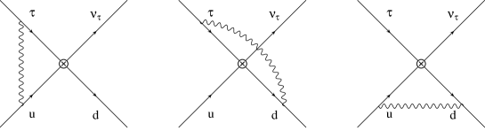
Figure 3: Electromagnetic corrections to the $\tau$ decay vertex.

produce a multiplicative renormalization of the Lagrangian, and give

$$C_{\tau}(m_{\tau})=1+{\alpha_{\rm em}\over\pi}\ln{M_{W}\over m_{\tau}}\approx 1.009.$$ (37)

The $\tau$ decay amplitude $\tau\to\nu_{\tau}X$, where $X$ is the final hadronic state, can be written as

$$A=-i{4G_{F}\over\sqrt{2}}C_{\tau}(\mu)\bar{u}(p_{\nu})\gamma^{\mu}P_{L}u(p_{\tau})\left[V_{ud}^{*}{\left\langle{X}\vphantom{\bar{d}\gamma_{\mu}P_{L}u0}\right|{\bar{d}\gamma_{\mu}P_{L}u}\left|\vphantom{X\bar{d}\gamma_{\mu}P_{L}u}{0}\right\rangle}+V_{us}^{*}{\left\langle{X}\vphantom{\bar{s}\gamma_{\mu}P_{L}u0}\right|{\bar{s}\gamma_{\mu}P_{L}u}\left|\vphantom{X\bar{s}\gamma_{\mu}P_{L}u}{0}\right\rangle}\right].$$ (38)

Squaring the amplitude, and computing the decay rate gives

$$\Gamma = 4{G_{F}^{2}\left|C_{\tau}\right|^{2}\left|V_{ud}\right|^{2}\over m_{\tau}}\sum_{X}\int{d^{3}p_{\nu}\over(2\pi)^{3}2E_{\nu}}\left[p_{\nu}^{\mu}p_{\tau}^{\nu}+p_{\nu}^{\nu}p_{\tau}^{\mu}-p_{\nu}\cdot p_{\tau}g^{\mu\nu}-i\epsilon^{\mu\nu}{}_{\alpha\beta}p_{\nu}^{\alpha}p_{\tau}^{\beta}\right]$$ (39)

$$\times(2\pi)^{4}\delta^{4}(p_{\tau}-p_{\nu}-p_{X}){\left\langle{0}\vphantom{\bar{u}\gamma_{\nu}P_{L}dX}\right|{\bar{u}\gamma_{\nu}P_{L}d}\left|\vphantom{0\bar{u}\gamma_{\nu}P_{L}d}{X}\right\rangle}{\left\langle{X}\vphantom{\bar{d}\gamma_{\mu}P_{L}u0}\right|{\bar{d}\gamma_{\mu}P_{L}u}\left|\vphantom{X\bar{d}\gamma_{\mu}P_{L}u}{0}\right\rangle},$$

where we have retained only the $V_{ud}$ term for simplicity. The sum on $X$ is symbolic for the sum over all final states, including phase space factors. The $\delta$ function can be written as

$$\delta^{4}(p_{\tau}-p_{\nu}-p_{X})=\int d^{4}q\delta^{4}(p_{\tau}-p_{\nu}-q)\delta^{4}(q-p_{X}),$$ (40)

and the sum on $X$ can be written as

$$\sum_{X}(2\pi)^{4}\delta^{4}(q-p_{X}){\left\langle{0}\vphantom{\bar{u}\gamma_{\nu}P_{L}dX}\right|{\bar{u}\gamma_{\nu}P_{L}d}\left|\vphantom{0\bar{u}\gamma_{\nu}P_{L}d}{X}\right\rangle}{\left\langle{X}\vphantom{\bar{d}\gamma_{\mu}P_{L}u0}\right|{\bar{d}\gamma_{\mu}P_{L}u}\left|\vphantom{X\bar{d}\gamma_{\mu}P_{L}u}{0}\right\rangle}=W_{\nu\mu}^{(ud)}(q).$$ (41)

The tensor $W_{\mu\nu}$ is related to another quantity $\Pi_{\mu\nu}$, defined by

$$\Pi_{\mu\nu}^{(ud)}(q)=-i\int{d^{4}q}e^{-iq\cdot x}{\left\langle{0}\vphantom{T(j_{\nu}^{\dagger}(x)j_{\mu}(0)0}\right|{T(j_{\nu}^{\dagger}(x)j_{\mu}(0)}\left|\vphantom{0T(j_{\nu}^{\dagger}(x)j_{\mu}(0)}{0}\right\rangle},$$ (42)

where $j^{\mu}=\bar{d}\gamma_{\mu}P_{L}u$. Inserting a complete set of states in the time-ordered product, one finds that

$$W_{\mu\nu}^{(ud)}=2\ {\rm Im\,}\Pi_{\mu\nu}^{(ud)}$$ (43)

The tensor $\Pi_{\mu\nu}$ depends on the only variable, $q$, and must have the form

$$\Pi_{\mu\nu}^{(ud)}(q)=\left(-q^{2}g_{\mu\nu}+q_{\mu}q_{\nu}\right)\Pi_{T}^{(ud)}(q^{2})+q_{\mu}q_{\nu}\Pi_{L}^{(ud)}(q^{2}),$$ (44)

by Lorentz invariance. The tensor $W_{\mu\nu}$ is then given by

$$W_{\mu\nu}^{(ud)}(q)=\left(-q^{2}g_{\mu\nu}+q_{\mu}q_{\nu}\right)\Omega_{T}^{(ud)}(q^{2})+q_{\mu}q_{\nu}\Omega_{L}^{(ud)}(q^{2}),$$ (45)

where

$$\Omega_{L}^{(ud)}=2\ {\rm Im\,}\Pi_{L}^{(ud)},\qquad\Omega_{T}^{(ud)}=2\ {\rm Im\,}\Pi_{T}^{(ud)}.$$ (46)

If the light quark mass difference $m_{d}-m_{u}$ and $m_{s}-m_{u}$ are neglected, the hadronic currents $\bar{d}\gamma_{u}P_{L}u$ and $\bar{s}\gamma_{u}P_{L}u$ are conserved. This implies that $q^{\mu}\Pi_{\mu\nu}=0$, so that $\Pi_{L}(q^{2})=0$. Inserting Eq. (40) and Eq. (45) into Eq. (47) gives

$$\Gamma = 2{G_{F}^{2}\left|C_{\tau}\right|^{2}\over m_{\tau}}\int d^{4}q\delta(p_{\tau}-p_{\nu}-q)\int{d^{3}p_{\nu}\over(2\pi)^{3}2E_{\nu}}$$ (47)

$$(m_{\tau}^{2}-q^{2})\left[\Omega_{T}(m_{\tau}^{2}+2q^{2})+\Omega_{L}m_{\tau}^{2}\right],$$

where

$$\Omega_{T,L}=\left|V_{ud}\right|^{2}\Omega_{T,L}^{(ud)}+\left|V_{us}\right|^{2}\Omega_{T,L}^{(us)}$$ (48)

and we added back the $V_{us}$ contribution. There is no interference term (at lowest order in the weak interactions), because the $u\to d$ and $u\to s$ currents lead to final states with different flavor quantum numbers, and the strong interactions conserve flavor. The hadronic invariant mass distribution can then be written as

$${d\Gamma\over ds} = {G_{F}^{2}\left|C_{\tau}\right|^{2}\over 8\pi^{2}m_{\tau}^{3}}(m_{\tau}^{2}-s)^{2}\left[\Omega_{T}(s)(m_{\tau}^{2}+2s)+\Omega_{L}(s)m_{\tau}^{2}\right]$$ (49)

The ratio of the hadronic to leptonic decay rate of the $\tau$ is given by  [100]

$$R_{\tau}=6\pi\left|C_{\tau}\right|^{2}\int_{0}^{m_{\tau}^{2}}{ds\over m_{\tau}^{2}}\left(1-{s\over m_{\tau}^{2}}\right)^{2}\left[\Omega_{T}(s)\left(1+{2s\over m_{\tau}^{2}}\right)+\Omega_{L}(s)\right]$$ (50)

The hadronic tensors $\Pi_{L,T}(s)$ are analytic in the complex $s$ plane, except for a branch cut along the positive real axis. The discontinuity across the cut is $\Omega_{L,T}(s)$, and is the cross-section for the currents to create hadrons. Clearly, the hadron production rate is sensitive to non-perturbative effects, and can not be computed reliably. Far away from the physical cut, there are no infrared singularities, and QCD perturbation theory is valid. One can rewrite the integral Eq. (50) as

$$R_{\tau}=6\pi i\int_{C}{ds\over m_{\tau}^{2}}\left(1-{s\over m_{\tau}^{2}}\right)^{2}\left[\Pi_{T}(s)\left(1+{2s\over m_{\tau}^{2}}\right)+\Pi_{L}(s)\right],$$ (51)

where $C=C_{1}$ is the contour shown in Fig. (4).

Figure 4: Integration contours $C_{1}$ and $C_{2}$ in the complex $s$ plane.

The difference of $\Pi_{L,T}$ above and below the cut is $\Omega_{L,T}$, so this gives back Eq. (50). Since $\Pi_{L,T}$ have no singularities in the complex $s$ plane other than the branch cut, one can deform the contour $C_{1}$ to the contour $C_{2}$, and use Eq. (51) with $C=C_{2}$. The advantage of using Eq. (51) with $C=C_{2}$ rather than $C=C_{1}$ is that one needs to know $\Pi_{L,T}$ far away from the cut for most of the integration contour. The contour approaches the cut at $s=m_{\tau}^{2}$, but at this point, the integrand vanishes as $(s-m_{\tau})^{2}$, so the contribution of the region near $s=m_{\tau}^{2}$ to the total integral is suppressed  [100].

$\Pi(s)$ can be computed in perturbation theory using an operator product expansion, which is valid away from the physical cut. The perturbation theory result for $\Pi(s)$ is then substituted in Eq. (51). In practice, the calculation can be simplified by using the perturbation theory value for $\Omega(s)$ in Eq. (50). We have argued above that perturbation theory is not valid for $\Omega(s)$. Nevertheless, using the perturbation theory value for $\Omega(s)$ in Eq. (50) is justified because $\Pi(s)$ in perturbation theory has the same analytic structure in QCD. Thus using the perturbation theory value of $\Pi(s)$ in Eq. (51) is equivalent to using the perturbation theory value for $\Omega(s)$ in Eq. (50), even though the perturbative computation of $\Omega(s)$ is not valid.

The OPE for $\Pi(s)$ is closely related to that for $e^{+}e^{-}\to{\rm hadrons}$, which depends on the time-ordered product of two electromagnetic currents.

$$\Pi(s)=c_{i}(\mu,s,\alpha_{s}(\mu))\left\langle{O_{i}(\mu)}\right\rangle,$$ (52)

where $c_{i}$ are the coefficient functions, and $O_{i}$ are the local operators. Since the contour $C_{2}$ is a circle of radius $m_{\tau}^{2}$ in the complex $s$ plane, one expects that logarithms in the uncalculated higher order corrections are minimized if one chooses $\mu=m_{\tau}$. The leading order operator is the unit operator. In the limit that the light quark masses are neglected, $\Pi_{L}$ vanishes, and we only need to compute $\Pi_{T}$, giving

$$2\pi\Omega_{T}(s) = \left|C_{\tau}\right|^{2}\left(\left|V_{ud}\right|^{2}+\left|V_{us}\right|^{2}\right)$$ (53)

$$\times\left[1+{\alpha_{s}(\sqrt{s})\over\pi}+F_{3}\left({\alpha_{s}(\sqrt{s})\over\pi}\right)^{2}+F_{4}\left({\alpha_{s}(\sqrt{s})\over\pi}\right)^{3}+\ldots\right].$$

The first coefficient is the well-known result that the ratio $\sigma(e^{+}e^{-}\to{\rm hadrons})/\sigma(e^{+}e^{-}\to q\bar{q})$ is $3(1+\alpha_{s}(\sqrt{s})/\pi)$. The next two coefficients are

$$F_{3}=1.9857-0.1153n_{f},\qquad F_{4}=-6.6368-1.2001n_{f}-0.0052n_{f}^{2}.$$ (54)

Using the $\beta$-function to write $\alpha_{s}(\sqrt{s})$ in terms of $\alpha_{s}(m_{\tau})$, evaluating the $s$ integral, and setting $n_{f}=3$ gives  [100]

$$R_{\tau} = 3\left|C_{\tau}\right|^{2}\left(\left|V_{ud}\right|^{2}+\left|V_{us}\right|^{2}\right)$$ (55)

$$\times\left[1+{\alpha_{s}(m_{\tau})\over\pi}+5.2023\left({\alpha_{s}(m_{\tau})\over\pi}\right)^{2}+26.366\left({\alpha_{s}(m_{\tau})\over\pi}\right)^{3}+\ldots\right]$$

Assuming $\alpha_{s}(m_{\tau})\approx 0.35$, the series in brackets is $1+0.111+0.065+0.036+\ldots$, so the terms are still numerically decreasing till order $\alpha^{3}$. One can use the value of the last term as an estimate of the theoretical uncertainty in the perturbative value for the coefficient of the unit operator. This also tells us that we can neglect corrections from higher dimension operator that are smaller than about $3\%$.

The $1/m_{\tau}^{2}$ corrections to $R_{\tau}$ arise from the quark mass corrections to the coefficient of the unit operator in the OPE. At order $m^{2}/m_{\tau}^{2}$, the currents are no longer conserved, so one needs to compute both $\Pi_{L}$ and $\Pi_{T}$. The only light quark mass contribution of any significance is the $s$-quark mass correction [100],

$$\delta R_{\tau}=3\left|V_{us}\right|^{2}\left[-8{m_{s}^{2}\over m_{\tau}^{2}}\left(1+{16\alpha_{s}(m_{\tau})\over 3\pi}\right)\right].$$ (56)

Using $m_{s}\sim 150$ MeV as an estimate for the $s$-quark mass gives $\delta R_{\tau}\sim-0.008$, which is smaller than the error in the perturbation series.

The $1/m_{\tau}^{4}$ and corrections in the OPE arise from the dimension four operators $F_{\mu\nu}F^{\mu\nu}$ and $m\bar{\psi}\psi$, and the $1/m_{\tau}^{6}$ corrections from the four-quark operators $\bar{\psi}\Gamma\psi\bar{\psi}\Gamma\psi$, where $\Gamma$ is some combination of $\gamma$ matrices. An analysis of these corrections, based on model estimates of the operator matrix elements indicates that these corrections are smaller than the uncertainty in the perturbation series [100]. The size of non-perturbative corrections can be determined directly from the experimental data. Instead of considering the integral Eq. (50) that gives the total hadronic width, one compares the integral of $d\Gamma/ds$ weighted with

$(1-s/m_{\tau}^{2})^{k}(s/m_{\tau}^{2})^{l}$ with the corresponding moment of the experimental data. By studying the moments for different values of $k$ and $l$, one finds that the non-perturbative corrections are about 3%  [103, 104], and so are comparable in size to the uncertainty in the perturbation series.

The experimentally measured quantity is $R_{\tau}^{(ud)}=3.484\pm 0.024$  [102, 103], the ratio for $\tau$ to decay into non-strange hadrons to the leptonic decay rate. This is given by Eq. (55), dropping $V_{us}$, and gives

$$\alpha_{s}(m_{\tau})=0.34\pm 0.03,$$ (57)

where we have assumed a theoretical uncertainty of 100% in the $\alpha^{3}$ term. This value corresponds to

$$\alpha_{s}(m_{Z})=0.119\pm 0.003,$$ (58)

7 $\alpha_{s}$ FROM LATTICE GAUGE THEORY COMPUTATIONS

The strong coupling constant $\alpha_{s}$ can be determined from lattice gauge theory calculations of the hadronic spectrum. The basic procedure used is to choose a definition of $\alpha_{s}$, and measure its value on the lattice. One then has to set the scale at which $\alpha_{s}$ takes on the measured value. The lattice scale can be normalized using the hadronic spectrum measured on the same lattice. Finally, one has to convert the lattice definition of $\alpha_{s}$ to the value defined in the continuum in a scheme such as $\overline{\rm MS}$.

There are several sources of systematic errors that limit the current accuracy in determining $\alpha_{s}$. Typically, $\alpha_{s}$ is determined by determining the spectrum of heavy quark bound states on the lattice. There are corrections due to the finite volume and finite lattice spacing $a$. The finite lattice spacing errors can be reduced by using improved actions, that are accurate to higher order in $a$. To some extent, one can estimate the error due to finite volume and finite lattice spacing by repeating the simulation on a larger lattice. The dominant systematic uncertainty is due to the quenched approximation, in which light quark loops are neglected. It is difficult to reliably estimate the systematic errors due to this approximation without doing a full simulation including dynamical fermions. Simulations with dynamical fermions are just starting to be done, and in a few years one should have more reliable estimates of $\alpha_{s}$.

There is one important advantage to using a heavy quark system such as the $\Upsilon$ to determine $\alpha_{s}$. The leading correction to the $\Upsilon$ energy levels due to the light quark masses is linear in the quark masses, and can only depend on the flavor singlet combination $m_{u}+m_{d}+m_{s}$. Thus the light quark mass corrections can be computed to a good approximation using three light quarks of mass $(m_{u}+m_{d}+m_{s})/3$. This avoids having to simulate almost massless dynamical quarks, which is very difficult.

Lattice calculations can also be used to test theoretical calculations, and determine the regime in which perturbation theory is applicable. In the quenched approximation, one can study the scale dependence of the coupling constant on the lattice. This provides a check on the perturbation theory calculation with $n_{f}=0$. The result is in remarkable agreement with the perturbation theory result in the regime where the coupling constant is weak  [105, 106].

The Fermilab and SCRI groups use the $S-P$ and $1S-2S$ splittings in the $\Upsilon$ system to determine $\alpha_{s}$. There are some systematic deviations of the calculated numbers from their experimental values in the quenched approximation ($n_{f}=0$), which are dramatically reduced if one includes $n_{f}=2$ dynamical flavors. The value of $\alpha_{s}(M_{Z})$ in the $\overline{\rm MS}$ scheme is  [107]

$$\alpha_{s}(M_{Z})=0.1159\pm 0.0019\pm 0.0013\pm 0.0019$$ (59)

where the first error is due to discretization effects, relativistic corrections, and statistical errors, the second is due to dynamical fermions, and the third is from conversion uncertainties.

More recent computations give (in the $n_{f}=5$ scheme)  [108]

$$\alpha_{s}(M_{Z})=0.1174\pm 0.0024$$ (60)

and  [109]

$$\alpha_{s}(M_{Z})=0.1118\pm 0.0017.$$ (61)

An average of these newer values gives $\alpha_{s}(M_{Z})=0.115\pm 0.004$, where we have included the difference between the two central values as an estimated additional systematic error.

8 $\alpha_{s}$ FROM HEAVY QUARK SYSTEMS

Heavy quark bound states such as the $\Upsilon$ can also be used to extract a value for $\alpha_{s}$. If the bound state is treated using non-relativistic quantum mechanics, the annihilation decays $\Upsilon\to\mu^{+}\mu^{-}$, $\Upsilon\to ggg$ and $\Upsilon\to\gamma gg$ can be computed as the product of the probability to find the quark-antiquark pair at the origin, times the annihilation rate for $Q\bar{Q}$ at rest to decay to the final state. The relevant Feynman graphs are shown in Fig. 5. The decay rate $\Upsilon\to ggg$ is the inclusive decay rate for $\Upsilon\to{\rm hadrons}$, and the decay rate for $\Upsilon\to\gamma gg$ is that for $\Upsilon\to\gamma+{\rm hadrons}$. The probability to find $Q\bar{Q}$ at the origin, $\left|\psi(0)\right|^{2}$, is sensitive to the detailed dynamics of the $Q\bar{Q}$ bound state. If one takes the ratio of decay rates, $\left|\psi(0)\right|^{2}$ drops out, and the ratio of decay rates can be used to determine $\alpha_{s}$.

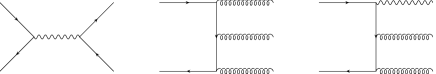
Figure 5: Decay diagrams for $\Upsilon\to\mu^{+}\mu^{-}$, $\Upsilon\to ggg$ and $\Upsilon\to\gamma gg$.

The above qualitative discussion can be made precise using NRQCD (non-relativistic QCD) to calculate the properties of the $\Upsilon$  [110]. NRQCD has an expansion in powers of $v$, the velocity of quarks in the bound state. The $\alpha_{s}$ expansion is coupled to the $v$ expansion, since $v\sim\alpha_{s}$ in a Coulombic system. The NRQCD approach allows one to systematically factor the decay rate into short distance coefficients that are calculable in perturbation theory, and non-perturbative hadronic matrix elements that generalize the notion of the wavefunction at the origin. The $\Upsilon$ wavefunction in NRQCD has different Fock components. The lowest order (in $v$) component is ${\left|{\bar{Q}Q}\right\rangle}$ and the first correction contains a gluon, ${\left|{\bar{Q}Qg}\right\rangle}$. The ${\left|{\bar{Q}Qg}\right\rangle}$ is referred to as the color-octet component, because the two quarks are in a color octet state. The NRQCD velocity counting rules show that the probability to find the $\Upsilon$ in the octet component is of order $v^{2}$.

The decay rate for $\Upsilon\to\mu^{+}\mu^{-}$ in NRQCD is  [110]

$$\Gamma(\Upsilon\to\mu^{+}\mu^{-})={2{\rm Im\,}f_{ee}({}^{3}S_{1})\over M^{2}_{b}}{\left\langle{\Upsilon}\vphantom{{\mathcal{O}}_{1}({}^{3}S_{1})\Upsilon}\right|{{\mathcal{O}}_{1}({}^{3}S_{1})}\left|\vphantom{\Upsilon{\mathcal{O}}_{1}({}^{3}S_{1})}{\Upsilon}\right\rangle}+{2{\rm Im\,}g_{ee}({}^{3}S_{1})\over M^{4}_{b}}{\left\langle{\Upsilon}\vphantom{{\mathcal{P}}_{1}({}^{3}S_{1})\Upsilon}\right|{{\mathcal{P}}_{1}({}^{3}S_{1})}\left|\vphantom{\Upsilon{\mathcal{P}}_{1}({}^{3}S_{1})}{\Upsilon}\right\rangle}$$ (62)

where $M_{b}$ is the $b$-quark pole mass, ${{\mathcal{O}}_{1}({}^{3}S_{1})}=\psi^{\dagger}\mbox{\boldmath$\sigma$}\chi\cdot\chi^{\dagger}\mbox{\boldmath$\sigma$}\psi$ and ${{\mathcal{P}}_{1}({}^{3}S_{1})}=-i/4(\psi^{\dagger}\mbox{\boldmath$\sigma$}\chi\cdot\chi^{\dagger}\mbox{\boldmath$\sigma$}(\raise 6.45831pt\hbox{$\leftrightarrow$}\mkern-16.5mu\bf D)^{2}\psi+{\rm h.c.})$, and $\psi$ and $\chi^{\dagger}$ annihilate quarks and antiquarks, respectively. The first term is the leading order contribution, and the second term is the $v^{2}$ correction. The coefficients $f_{ee}({}^{3}S_{1})$ and $g_{ee}({}^{3}S_{1})$ can be computed from the first graph in Fig. 5 at lowest order in perturbation theory. The values are  [110]

$${\rm Im\,}f_{ee}({}^{3}S_{1})={\pi\alpha^{2}e_{b}^{2}\over 3}\left[1-16{\alpha_{s}\over\pi}\right],\qquad{\rm Im\,}g_{ee}({}^{3}S_{1})=-{4\pi\alpha^{2}e_{b}^{2}\over 9},$$ (63)

where $e_{b}=-1/3$ is the charge of the $b$-quark, and the radiative correction to $f_{ee}({}^{3}S_{1})$ has also been included.

The decay rate for $\Upsilon\to{\rm hadrons}$ is  [110]

$$\Gamma(\Upsilon\to{\rm hadrons}) = {2{\rm Im\,}f_{1}({}^{3}S_{1})\over M^{2}_{b}}{\left\langle{\Upsilon}\vphantom{{\mathcal{O}}_{1}({}^{3}S_{1})\Upsilon}\right|{{\mathcal{O}}_{1}({}^{3}S_{1})}\left|\vphantom{\Upsilon{\mathcal{O}}_{1}({}^{3}S_{1})}{\Upsilon}\right\rangle}+{2{\rm Im\,}g_{1}({}^{3}S_{1})\over M^{4}_{b}}{\left\langle{\Upsilon}\vphantom{{\mathcal{P}}_{1}({}^{3}S_{1})\Upsilon}\right|{{\mathcal{P}}_{1}({}^{3}S_{1})}\left|\vphantom{\Upsilon{\mathcal{P}}_{1}({}^{3}S_{1})}{\Upsilon}\right\rangle}$$ (64)

$$+\Gamma^{(8)}(\Upsilon\to{\rm hadrons})$$

where $\Gamma^{(8)}$ is the contribution to the decay rate from the color-octet component of the $\Upsilon$. In NRQCD, the color octet decay rate is $v^{4}$ suppressed relative to the color singlet decay rate. However, the color octet component can decay into two gluons, rather than three, so the color octet decay rate of order $\alpha_{s}^{2}v^{4}$ can compete with the relativistic correction to the color singlet decay rate of order $\alpha_{s}^{3}v^{2}$. The coefficient functions are  [110]

$${\rm Im\,}f_{1}({}^{3}S_{1}) = {10\over 243}(\pi^{2}-9)\alpha_{s}^{3}(M_{b})$$

$$\times\left[1+\left(-9.46(2)C_{F}+4.13(17)C_{A}-1.161(2)n_{f}){\alpha_{s}\over\pi}\right)\right]$$

$${\rm Im\,}g_{1}({}^{3}S_{1}) = -{5\over 1458}(19\pi^{2}-132)\alpha_{s}^{3}(M_{b})$$ (65)

The $\alpha_{s}^{3}$ term for ${\rm Im\,}f_{1}({}^{3}S_{1})$ has the given value when the scale of the $\alpha_{s}^{2}$ term is the $b$-quark pole mass.

The decay rate $\Gamma(\Upsilon\to\gamma+{\rm hadrons})$ has the form

$$\Gamma(\Upsilon\to\gamma+{\rm hadrons})={2{\rm Im\,}f_{\gamma}({}^{3}S_{1})\over M_{b}^{2}}{\left\langle{\Upsilon}\vphantom{{\mathcal{O}}_{1}({}^{3}S_{1})\Upsilon}\right|{{\mathcal{O}}_{1}({}^{3}S_{1})}\left|\vphantom{\Upsilon{\mathcal{O}}_{1}({}^{3}S_{1})}{\Upsilon}\right\rangle}+{2{\rm Im\,}g_{\gamma}({}^{3}S_{1})\over M_{b}^{2}}{\left\langle{\Upsilon}\vphantom{{\mathcal{P}}_{1}({}^{3}S_{1})\Upsilon}\right|{{\mathcal{P}}_{1}({}^{3}S_{1})}\left|\vphantom{\Upsilon{\mathcal{P}}_{1}({}^{3}S_{1})}{\Upsilon}\right\rangle},$$ (66)

where the coefficient function is  [110]

$${\rm Im\,}f_{\gamma}({}^{3}S_{1}) = {8\over 27}(\pi^{2}-9)\alpha_{s}^{2}(M_{b})\alpha e_{b}^{2}$$ (67)

$$\times\left[1+\left(-9.46(2)C_{F}+2.75(11)C_{A}-0.774(1)n_{f}){\alpha_{s}\over\pi}\right)\right]$$

The equations of motion can be used to relate the matrix elements of the $S$-wave and $P$-wave operators  [111],

$${\left\langle{\Upsilon}\vphantom{{\mathcal{P}}_{1}({}^{3}S_{1})\Upsilon}\right|{{\mathcal{P}}_{1}({}^{3}S_{1})}\left|\vphantom{\Upsilon{\mathcal{P}}_{1}({}^{3}S_{1})}{\Upsilon}\right\rangle}={M_{\Upsilon}-M_{b}\over M_{b}}{\left\langle{\Upsilon}\vphantom{{\mathcal{O}}_{1}({}^{3}S_{1})\Upsilon}\right|{{\mathcal{O}}_{1}({}^{3}S_{1})}\left|\vphantom{\Upsilon{\mathcal{O}}_{1}({}^{3}S_{1})}{\Upsilon}\right\rangle}+O(v^{2}).$$ (68)

The matrix element of the $S$-wave operator is the NRQCD analog of the wavefunction at the origin in a potential model calculation. The matrix element is non-perturbative, and can be eliminated by considering ratios of decay rates. The matrix element of ${\mathcal{P}}_{1}({}^{3}S_{1})$ can be determined from Eq. (68) using estimates of the $b$-quark pole mass $M_{b}$, and the measured $\Upsilon$ mass, as was done in Ref.  [111]. However, one can instead replace $(M_{\Upsilon}-2M_{b})/M_{b}$ by $-4/9\alpha_{s}^{2}$, the lowest-order result for the binding energy for a Coulomb bound state. This reduces somewhat the uncertainty in the extraction of $\alpha_{s}$, since it eliminates any uncertainty from the pole mass.

The experimental value of the ratio $\Gamma(\Upsilon\to{\rm hadrons})/\Gamma(\Upsilon\to\ell^{+}\ell^{-})=39.11\pm 0.4$  [112], where $\ell=e,\mu,\tau$ gives $\alpha_{s}(M_{b})=0.177\pm 0.01$, using the ratio of the theoretical formula for the decay widths. The unknown octet decay rate has been estimated to be less than 9% in Ref.  [111], and this has been included as a theoretical uncertainty. The decay rates Eq. (62)–(66) have been written in terms of $\alpha_{s}(M_{b})$. One can instead rewrite them in terms of $\alpha_{s}(\mu)$ using Eq. (8), extract $\alpha_{s}(\mu)$, and convert this into $\alpha_{s}(M_{b})$ using Eq. (8). We have include the uncertainty of a scale change by a factor of two in the theoretical estimate. The octet and scale uncertainties are comparable in size.

The experimental value of the ratio $\Gamma(\Upsilon\to\gamma+{\rm hadrons})/\Gamma(\Upsilon\to{\rm hadrons})=2.75\pm 0.04\pm 0.15$  [113] can also be used to extract $\alpha_{s}$. It is convenient to use the experimental value of $\Gamma(\Upsilon\to{\rm hadrons})/\Gamma(\Upsilon\to\ell^{+}\ell^{-})$ to convert this to $\Gamma(\Upsilon\to\gamma+{\rm hadrons})/\Gamma(\Upsilon\to\ell^{+}\ell^{-})=1.075\pm 0.06$, before comparing with the theoretical results. This eliminates the theoretical uncertainty due to the octet component in the hadronic decay rate. The extracted value of $\alpha_{s}(M_{b})$ is $0.189\pm 0.01$, where we have included a scale uncertainty as above. Averaging the two extractions gives $\alpha_{s}(M_{b})=0.183\pm 0.01$ which corresponds to $\alpha_{s}(M_{Z})=0.108\pm 0.004$

9 $\alpha_{s}$ FROM HADRON-HADRON SCATTERING

There are many process at high-energy hadron-hadron colliders which can constrain the value of $\alpha_{s}$. All rely on the QCD improved parton model, and on the factorization theorems of QCD  [114]. The rate for any process is expressed as a convolution of the partonic scattering amplitude $\sigma_{i,j}^{p}$ and parton distribution functions discussed in section 3; see Eq 28 (note that here we use $f$ rather than $q$ as the sum on $i,j$ runs over quarks and gluons.

$$\sigma=\sum_{i,j}\int\!dx_{1}dx_{2}f_{i}(x,M^{2})f_{j}(x,M^{2})\sigma_{ij}^{p}(M)$$ (69)

The factorization scale $M$ is arbitrary. As in the case of the scale $\mu$ used in $\alpha_{s}(\mu)$ (see Eq 10 and the surrounding discussion), the exact result cannot depend on its choice. However as the processes $\sigma_{i,j}^{p}$ is only calculated to some finite order in perturbation theory, some residual $M$ dependence will remain. As in the case of $\mu$ the sensitivity to $M$ will be small if it is chosen to be a characteristic scale of the process; for example, in the case of the production of a pair of jets of momentum, $p_{T}$, transverse to the direction defined by the incoming hadrons, $M=p_{T}$ is a reasonable choice.

The quantitative tests of QCD and the consequent extraction of $\alpha_{s}$ which appears in $\sigma_{i,j}^{p}$ are possible only if the process in question has been calculated beyond leading order in QCD perturbation theory. The production of hadrons with large transverse momentum in hadron-hadron collisions provides a direct probe of the scattering of quarks and gluons: $qq\to qq$, $qg\to qg$, $gg\to gg$, etc.. Here the leading order term in $\sigma_{i,j}^{p}$ is of order $\alpha_{s}^{2}$ so the rates are sensitive to its value. Higher–order QCD calculations of the jet rates [115] and shapes are in impressive agreement with data [116]. This agreement has led to the proposal that these data could be used to provide a determination of $\alpha_{s}$ [117]. A set of structure functions is assumed and Tevatron collider data are fitted over a very large range of transverse momenta, to the QCD prediction for the underlying scattering process that depends on $\alpha_{s}$. The evolution of the coupling over this energy range (40 to 250 GeV) is therefore tested in the analysis. CDF obtains $\alpha_{s}(M_{Z})=0.1129\pm 0.0001~{}(\hbox{stat.})\pm 0.0085~{}(\hbox{syst.})$  [118]. Estimation of the theoretical errors is not straightforward. The structure functions used depend implicitly on $\alpha_{s}$ and an iteration procedure must be used to obtain a consistent result; different sets of structure functions yield different correlations between the two values of $\alpha_{s}$. We estimate an uncertainty of $\pm 0.005$ from examining the fits. Ref.  [117] estimates the error from unknown higher order QCD corrections to be $\pm 0.005$. Combining these then gives: $\alpha_{s}(M_{Z})=0.1129\pm 0.011$

QCD corrections to Drell-Yan type cross sections (the production in hadron collisions by quark-antiquark annihilation of lepton pairs of invariant mass $Q$ from virtual photons or of real $W$ or $Z$ bosons), are known [119]. These processes are not very sensitive to $\alpha_{s}$ as the leading piece in $\sigma_{i,j}^{p}$ is of order $\alpha_{s}^{0}$. The production of $W$ and $Z$ bosons and photons at large transverse momentum begins at order $\alpha_{s}^{0}$. The leading-order QCD subprocesses are $q\overline{q}\to\gamma g$ and $qg\to\gamma q$. The next-to-leading-order QCD corrections are known [120] [121] for photons, and for $W/Z$ production [122], and so an extraction of $\alpha_{s}$ is possible in principle.

Data exist on photon production from the CDF and DØ collaborations [123] [124] and from fixed target experiments  [125]. Detailed comparisons with QCD predictions  [126] may indicate an excess of the data over the theoretical prediction at low value of transverse momenta, although other authors  [127] find smaller excesses. These differences indicate that while the process may be understood, no meaningful extraction of $\alpha_{s}$ is possible.

The UA2 collaboration [128] has extracted a value of $\alpha_{s}(M_{W})=0.123\pm 0.018(\hbox{stat.})\pm 0.017(\hbox{syst.})$ from the measured ratio $R_{W}={\sigma(W+1\hbox{jet})}/{\sigma(W+0\hbox{jet})}$. The result depends on the algorithm used to define a jet, and the dominant systematic errors due to fragmentation and corrections for underlying events (the former causes jet energy to be lost, the latter causes it to be increased) are connected to the algorithm. The scale at which $\alpha_{s}(M)$ is to be evaluated is not clear. A change from $\mu=M_{W}$ to $\mu=M_{W}/2$ causes a shift of 0.01 in the extracted $\alpha_{s}$, and the quoted error should be increased to take this into account. There is also dependence on the parton distribution functions, and hence, $\alpha_{s}$ appears explicitly in the formula for $R_{W}$, and implicitly in the distribution functions. Data from CDF and DØ on the W $p_{T}$ distribution  [129] are in agreement with QCD but are not able to determine $\alpha_{s}$ with sufficient precision to have any weight in a global average.

The production rates of $b$ quarks in $p\overline{p}$ have been used to determine $\alpha_{s}$  [132]. The next to leading order QCD production processes  [131] have been used. At order $\alpha_{s}$ the production processes are $gg\to b\overline{b}$ and $q\overline{q}\to b\overline{b}$ result in b-hadrons that are back to back in azimuth. By selecting events in this region the next-to leading order calculation can be used to compare rates to the measured value and a value of $\alpha_{s}$ extracted. The errors are dominated by the measurement errors, the choice of $\mu$ and $M$, and uncertainties in the choice of structure functions. The last were estimated by varying the structure functions used. The result is $\alpha_{s}(M_{Z})=0.113^{+0.009}_{-0.013}$.

10 CONCLUSION

The previous sections have illustrated the large number of processes where quantitative tests of QCD can be made and a value of $\alpha_{s}$ extracted. Figure 6 shows the values of $\alpha_{s}(M_{Z})$ deduced from the various processes shown above. The consistency and precision of these results is remarkable. Figure 7 shows the values of $\alpha_{s}(\mu)$ and the values of $\mu$ where they are measured. This figure clearly shows the experimental evidence for the variation of $\alpha_{s}(\mu)$ with $\mu$ predicted by Eq.4.

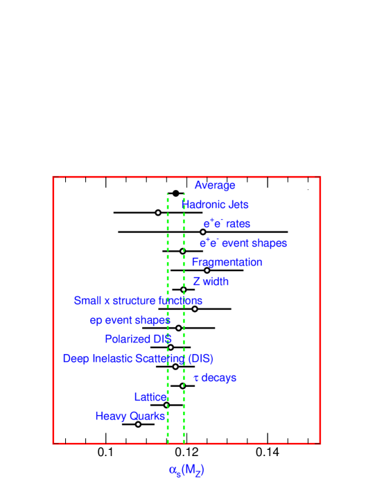
Figure 6: Summary of $\alpha_{s}(M_{Z})$

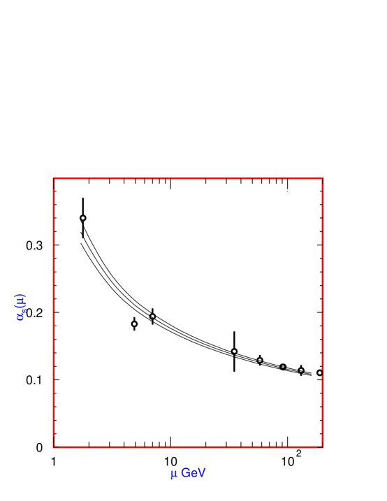
Figure 7: Values of $\alpha_{s}(\mu)$ and the values of $\mu$ where they are measured. these results are, in increasing value of $\mu$, $\tau$ width, heavy quark decays, deep inelastic at $\sqrt{<Q^{2}>}=7$ GeV, $e^{+}e^{-}$ annihilation rate at 35 GeV, $e^{+}e^{-}$ event shapes at 58 GeV, the hadronic $Z$ width, $e^{+}e^{-}$ event shapes at Z, 130 and at 189 GeV. The lines show our average and $1\sigma$ errors.

An average of the values in Figure 6 and in Table 1 gives $\alpha_{s}(M_{z})=0.1173$, with a total $\chi^{2}$ of 9 for twelve fitted points, showing good consistency among the data. The value from heavy quark systems contributes slightly more that one half of the total $\chi^{2}$. If this result is omitted the average increases to 0.1185. All of the other results are within $1.1\sigma$ of the average value. The error on the average, assuming that all of the errors in the contributing results are uncorrelated, is $\pm 0.0014$, and may be an underestimate. We have seen that in almost all of the cases discussed, the errors are dominated by systematic, usually theoretical errors. Only some of these, notably from the choice of scale, are correlated. it is important to note that the average is not dominated by a single measurement; there are many results with comparable small errors: from $\tau$ decay, lattice gauge, theory deep inelastic scattering and the $Z^{0}$ width. We quote our average value as $\alpha_{s}(M_{Z})=0.1173\pm 0.002$, which corresponds to $\Lambda^{(5)}=200^{+24}_{-23}$ MeV using Eq. 13. The reader may wish to consult other recent articles for different opinions [133, 134].

Significant improvements in the precision in the near future are not likely. The accuracy of data from LEP will not improve. It is possible that a better understanding of the jet rates in hadron-hadron colliders and a systematic treatment of the errors from the structure functions will lead to and improvement in the precision of the value of $\alpha_{s}$ derived. In many cases where the data are quite precise, such as heavy quark system, theoretical uncertainties limit the precision. In the very long term precision at the 1% level may be achievable [135].

References

- 1. H. D. Politzer, Phys. Rev. Lett. 30: 1346 (1973); D. J. Gross and F. Wilczek, Phys. Rev. D9: 980 (1974)
- 2. R. D. Peccei and H. R. Quinn, Phys. Rev. Lett. 38: 1440 (1977); S. Weinberg, Phys. Rev. Lett. 37: 657 (1977)
- 3. W.A. Bardeen et al., Phys. Rev. D18: 3998 (1978)
- 4. G. Grunberg, Phys. Lett. 95B: 70 (1980); Phys. Rev. D29: 2315 (1984);P.M. Stevenson, Phys. Rev. D23: 2916 (1981); and Nucl. Phys. B203: 472 (1982); S. Brodsky and H.J. Lu, SLAC-PUB-6389 (Nov. 1993); S. Brodsky, G.P. Lepage, and P.B. Mackenzie, Phys. Rev. D28: 228 (1983)
- 5. S.A. Larin, T. van Ritbergen, and J.A.M. Vermaseren, Phys. Lett. B400: 379 (1997)
- 6. K. G. Chetyrkin, B. A. Kniehl and M. Steinhauser, Nucl. Phys. B510: 61 (1998)
- 7. K. Wilson Phys. Rev. 179: 1499 (1969)
- 8. B. Lautrup, Phys. Lett. B69: 109 (1977)
- 9. G. ’t Hooft, in The Whys of Subnuclear Physics, ed. by A.Zichichi, (Plenum, New York, 1978)
- 10. F. David, Nucl. Phys. B209: 433 (1982), Nucl. Phys. B234: 237 (1984)
- 11. I.I. Bigi, M. Shifman, N.G. Uraltsev and A. Vainshtein, Phys. Rev. D50: 2234 (1994)
- 12. M. Beneke and V. Braun, Nucl. Phys. B426: 301 (1994)
- 13. M. Beneke,Phys. Reports 317: 1 (1999)
- 14. T. D. Lee and M. Nauenberg, Phys. Rev. 133: B1549 (1964); T. Kinoshita, J. Math. Phys. 3 650 (1962)
- 15. A. Sinkovics, R. Akhoury and V. I. Zakharov, Phys. Rev. D58: 114025 (1998)
- 16. S.G. Gorishny, A. Kataev, and S.A. Larin, Phys. Lett. B259: 114 (1991) L.R. Surguladze and M.A. Samuel, Phys. Rev. Lett. 66: 560 (1991)
- 17. K.G. Chetyrkin and J.H. Kuhn, Phys. Lett. B308: 127 (1993)
- 18. R. Ammar et al., Phys. Rev. D57: 1350 (1998)
- 19. D. Haidt, in Directions in High Energy Physics, vol. 14, p. 201, ed. P. Langacker (World Scientific, 1995)
- 20. G. Quast, presented at the European Physical Society Meeting, Tampere, Finland (July 1999)
- 21. A. Blondel and C. Verzegrassi, Phys. Lett. B311: 346 (1993) G. Altarelli et al., Nucl. Phys. B405: 3 (1993)
- 22. J. Erler and P Langacker, Brief review in Eur.Phys.J.C3:1-794,1998.
- 23. V.N. Gribov and L.N. Lipatov, Sov. J. Nucl. Phys. 15: 438 (1972) Yu.L. Dokshitzer, Sov. Phys. JETP 46: 641 (1977)
- 24. G. Altarelli and G. Parisi, Nucl. Phys. B126: 298 (1977)
- 25. G. Curci, W. Furmanski, and R. Petronzio, Nucl. Phys. B175: 27 (1980) R. Petronzio, Phys. Lett. 97B: 437 (1980); and Z. Phys. C11: 293 (1982) E.G. Floratos, C. Kounnas, and R. Lacaze, Phys. Lett. 98B: 89 (1981); Phys. Lett. 98B: 285 (1981); and Nucl. Phys. B192: 417 (1981) R.T. Herrod and S. Wada, Phys. Lett. 96B: 195 (1981); and Z. Phys. C9: 351 (1981)
- 26. M. Glück et al., Z. Phys. C13: 119 (1982)
- 27. G. Sterman, Nucl. Phys. B281: 310 (1987) S. Catani and L. Trentadue, Nucl. Phys. B327: 323 (1989); Nucl. Phys. B353: 183 (1991)
- 28. D. Gross and C.H. Llewellyn Smith, Nucl. Phys. B14: 337 (1969)
- 29. J. Chyla and A.L. Kataev, Phys. Lett. B297: 385 (1992)
- 30. S.A. Larin and J.A.M. Vermaseren, Phys. Lett. B259: 345 (1991)
- 31. A.L. Kataev and V.V. Starchenko, Mod. Phys. Lett. A10: 235 (1995)
- 32. V.M. Braun and A.V. Kolesnichenko, Nucl. Phys. B283: 723 (1987)
- 33. M. Dasgupta and B. Webber, Phys. Lett. B382: 273 (1993)
- 34. J. Kim et al., Phys. Rev. Lett. 81: 3595 (1998)
- 35. D. Allasia et al., Z. Phys. C28: 321 (1985) K. Varvell et al., Z. Phys. C36: 1 (1997) V.V. Ammosov et al., Z. Phys. C30: 175 (1986) P.C. Bosetti et al., Nucl. Phys. B142: 1 (1978)
- 36. A.L. Kataev et al., hep-ph9907310
- 37. L.W. Whitlow et al., Phys. Lett. B282: 475 (1992)
- 38. A.C. Benvenuti et al., Phys. Lett. B223: 490 (1989); Phys. Lett. B223: 485, (1989); Phys. Lett. B237: 592 (1990); and Phys. Lett. B237: 599 (1990)
- 39. M.R. Adams et al., Phys. Rev. D54: 3006 (1996)
- 40. M. Derrick et al., Phys. Lett. B345: 576 (1995); Z. Phys. C62: 399 (1999)
- 41. J. Santiago and F.J. Yndurain, hep-ph/9904344
- 42. K. Adel, F. Barriero, and F.J. Yndurain, Nucl. Phys. B495: 221 (1997) W.L. Van Neerven, and E.B. Zijlstra, Phys. Lett. B272: 127 (1991); Nucl. Phys. B383: 525 (1992) S. A. Larin et al., Nucl. Phys. B427: 41 (1994); Nucl. Phys. B492: 338 (1997)
- 43. K. Bazizi and S.J. Wimpenny, UCR/DIS/91-02
- 44. M. Virchaux and A. Milsztajn, Phys. Lett. B274: 221 (1992)
- 45. P.Z. Quintas, Phys. Rev. Lett. 71: 1307 (1993)
- 46. K. Abe et al., Phys. Rev. Lett. 74: 346 (1995); Phys. Lett. B364: 61 (1995); Phys. Rev. Lett. 75: 25 (1995)
- 47. B. Adeva et al., Phys. Rev. D58: 112002 (1998)
- 48. D. Adams et al., Phys. Lett. B329: 399 (1995); Phys. Rev. D56: 5330 (1998); Phys. Rev. D58: 1112001 (1998)
- 49. A. Airapetian et al., Phys. Lett. B442: 484 (1998), hep-ex/99-06035
- 50. J.D. Bjorken, Phys. Rev. 148: 1467 (1966)
- 51. R. Mertig and W. L. van Neerven, Z. Phys. C70: 637 (1996)
- 52. G. Altarelli et al., Nucl. Phys. B496: 337 (1997), hep-ph/9803237
- 53. J. Ellis et al., Phys. Rev. D54: 6986 (1996)
- 54. A. DeRujula et al., Phys. Rev. D10: 1669 (1974) E.A. Kurayev, L.N. Lipatov, and V.S. Fadin, Sov. Phys. JETP 45: 119 (1977). Ya.Ya. Balitsky and L.N. Lipatov, Sov. J. Nucl. Phys. 28: 882 (1978)
- 55. R.D. Ball and S. Forte, Phys. Lett. B335: 77 (1994); Phys. Lett. B336: 77 (1994) H1Collaboration: S. Aid et al., Nucl. Phys. B470: 3 (1996)
- 56. R.D. Ball and A. DeRoeck, hep-ph/9609309European Physical Society meeting, Brussels, (July 1995)
- 57. H1 Collaboration: T. Ahmed et al., Nucl. Phys. B439: 471 (1995)
- 58. S. Catani and F. Hautmann, Nucl. Phys. B427: 475 (1994)
- 59. H.L. Lai et al., hep-ph/9903282A.D. Martin et al., hep-ph/9906231
- 60. E. Witten, Nucl. Phys. B120: 189 (1977)
- 61. J. Butterworth, International Conference on Lepton Photon Interactions, Stanford, USA (Aug. 1999)
- 62. K. Ackerstaff et al., Phys. Lett. B412: 225 (1997); Phys. Lett. B411: 387 (1997) P. Abreu et al., Z. Phys. C69: 223 (1996) R. Barate et al., Phys. Lett. B458: 152 (1999) M. Acciarri et al., Phys. Lett. B436: 403 (1998), L3 preprint 204 (2000)
- 63. K. Muramatsu et al., Phys. Lett. B332: 477 (1994)
- 64. S.K. Sahu et al., Phys. Lett. B346: 208 (1995)
- 65. H1 Collaboration: C. Adloff et al., DESY-98-205 J.Breitweg et al., DESY 99-057
- 66. S. Frixone, Nucl. Phys. B507: 295 (1997) B.W. Harris and J.F. Owens, Phys. Rev. D56: 4007 (1997) M. Klasen and G. Kramr, Z. Phys. C72: 107 (1996)
- 67. P. Nason and B.R. Webber, Nucl. Phys. B421: 473 (1994)
- 68. D. Buskulic et al., Phys. Lett. B357: 487 (1995) ibid., erratum Phys. Lett. B364: 247 (1995)
- 69. OPAL Collaboration: R. Akers et al., Z. Phys. C68: 203 (1995)
- 70. DELPHI Collaboration: P. Abreu et al., Phys. Lett. B398: 194 (1997)
- 71. E. Farhi, Phys. Rev. Lett. 39: 1587 (1977)
- 72. C.L. Basham et al., Phys. Rev. D17: 2298 (1978)
- 73. B. Andersson et al., Phys. Reports 97: 33 (1983) A. Ali et al., Nucl. Phys. B168: 409 (1980) A. Ali and R. Barreiro, Phys. Lett. 118B: 155 (1982) B.R. Webber, Nucl. Phys. B238: 492 (1984) G. Marchesini et al., Phys. Comm. 67, 465 (1992) T. Sjostrand and M. Bengtsson, Comp. Phys. Comm. 43: 367 (1987) T. Sjostrand, CERN-TH-7112/93 (1993)
- 74. S. Bethke et al., Phys. Lett. B213: 235 (1988)
- 75. S. Bethke et al., Nucl. Phys. B370: 310 (1992)
- 76. M.Z. Akrawy et al., Z. Phys. C49: 375 (1991)
- 77. K. Abe et al., Phys. Rev. Lett. 71: 2578 (1993); Phys. Rev. D51: 962 (1995)
- 78. P.D. Acton et al., Z. Phys. C55: 1 (1992); Z. Phys. C58: 386 (1993)
- 79. O. Adriani et al., Phys. Lett. B284: 471 (1992)
- 80. D. Decamp et al., Phys. Lett. B255: 623 (1992); Phys. Lett. B257: 479 (1992)
- 81. J. Ellis, M.K. Gaillard, and G. Ross, Nucl. Phys. B111: 253 (1976) ibid., erratum Nucl. Phys. B130: 516 (1977) P. Hoyer et al., Nucl. Phys. B161: 349 (1979)
- 82. R.K. Ellis, D.A. Ross, T. Terrano, Phys. Rev. Lett. 45: 1226 (1980) Z. Kunszt and P. Nason, ETH-89-0836 (1989)
- 83. O. Adriani et al., Phys. Lett. B284: 471 (1992) M. Akrawy et al., Z. Phys. C47: 505 (1990) B. Adeva et al., Phys. Lett. B248: 473 (1990) D. Decamp et al., Phys. Lett. B255: 623 (1991)
- 84. Y.L. Dokshitzer and B.R. Webber Phys. Lett. B352: 451 (1995) Y.L. Dokshitzer et. al. Nucl. Phys. B511: 396 (1997) Y.L. Dokshitzer et. al. JHEP 9801,011 (1998)
- 85. DELPHI Collaboration: Phys. Lett. B456: 322 (1999)
- 86. S. Catani et al., Phys. Lett. B263: 491 (1991)
- 87. S. Catani et al., Phys. Lett. B269: 432 (1991) S. Catani, B.R. Webber, and G. Turnock, Phys. Lett. B272: 368 (1991) N. Brown and J. Stirling, Z. Phys. C53: 629 (1992)
- 88. G. Catani et al., Phys. Lett. B269: 632 (1991); Phys. Lett. B295: 269 (1992); Nucl. Phys. B607: 3 (1993); Phys. Lett. B269: 432 (1991)
- 89. Y. Ohnishi et al., Phys. Lett. B313: 475 (1993)
- 90. L. Gibbons et al., CLNS 95-1323 (1995)
- 91. DELPHI Collaboration: D. Buskulic et al., Z. Phys. C73: 409 (1997); Z. Phys. C73: 229 (1997)
- 92. ALEPH Collaboration: 99-023 (1999); DELPHI Collaboration: 99-114 (1999); L3 Collaboration: L3-2414 (1999); OPAL Collaboration, PN-403 (1999); all submitted to International Conference on Lepton Photon Interactions,Stanford, USA (Aug. 1999)
- 93. OPAL Collaboration: M. Acciarri et al., Phys. Lett. B371: 137 (1996); Z. Phys. C72: 191 (1996) K. Ackerstaff et al., Z. Phys. C75: 193 (1997) ALEPH Collaboration: ALEPH 98-025 (1998)
- 94. JADE and OPAL Collaborations CERN/EP-99-175.
- 95. P. Abreu et al., Z. Phys. C59: 21 (1993), CERN-EP/99-133
- 96. D. Graudenz, Phys. Rev. D49: 3921 (1994) hep-ph/9708362J.G. Korner, E. Mirkes, and G.A. Schuler, Int. J. Mod. Phys. A4: 1781, (1989) S. Catani and M. Seymour, Nucl. Phys. B485: 291 (1997) M. Dasgupta and B.R. Webber, hep-ph/9704297E. Mirkes and D. Zeppenfeld, Phys. Lett. B380: 205 (1996)
- 97. H1 Collaboration: T. Ahmed et al., Phys. Lett. B346: 415 (1995); Europhys. J. C5: 575 (1998)
- 98. ZEUS Collaboration: M. Derrick et al., Phys. Lett. B363: 201 (1995)
- 99. S. Narison and A. Pich, Phys. Lett. B211: 183 (1988)
- 100. E. Braaten, S. Narison, and A. Pich, Nucl. Phys. B373: 581 (1992)
- 101. E. Braaten, Phys. Rev. Lett. 60: 1606 (1988)
- 102. T. Coan et al.(CLEO Collaboration), Phys. Lett. B356: 580 (1995)
- 103. ALEPH Collaboration, Europhys. J. C4: 409 (1998)
- 104. OPAL Collaboration, Europhys. J. C7: 571 (1999)
- 105. G. de Divitiis et al., Nucl. Phys. B437: 447 (1995)
- 106. M. Luscher et al., Nucl. Phys. B413: 481 (1994)
- 107. J. Shigemitsu, Nucl. Phys. B (Proc. Supp.) 53, 16 (1997)
- 108. C.T.H. Davies et al., Phys. Rev. D56: 2755 (1997)
- 109. A. Spitz et al. [SESAM Collaboration], Phys. Rev. D60: 074502 (1999)
- 110. G. T. Bodwin, E. Braaten and G. P. Lepage, Phys. Rev. D51: 1125 (1995)
- 111. M. Gremm and A. Kapustin, Phys. Lett. B407: 323 (1997)
- 112. Particle Data Group, Europhys. J. C3: 1 (1998)
- 113. B. Nemati et al., Phys. Rev. D55: 5273 (1997)
- 114. A. H. Mueller, Phys. Rev. D18: 3705 (1978) J. Collins, D. Soper and G. Sterman, Nucl. Phys. B223: 81 (1983), Phys. Lett. 109B: 388 (1983) R. K. Ellis, Nucl. Phys. B152: 285 (1979). Collins JC, Soper DE, Sterman G. in Perturbative Quantum Chromodynamics, edited by A. H. Mueller (World Scientific Singapore), p. 1.
- 115. S.D. Ellis, Z. Kunszt, and D.E. Soper, Phys. Rev. Lett. 64: 2121 (1990) F. Aversa et al., Phys. Rev. Lett. 65: 401 (1990) W.T. Giele, E.W.N. Glover, and D. Kosower, Phys. Rev. Lett. 73: 2019 (1994) S. Frixione, Z. Kunszt, and A. Signer, Nucl. Phys. B467: 399 (1996)
- 116. F. Abe et al., Phys. Rev. Lett. 77: 438 (1996) B. Abbott et al., Phys. Rev. Lett. 82: 2451 (1999)
- 117. W.T. Giele, E.W.N. Glover, and J. Yu, Phys. Rev. D53: 120 (1996)
- 118. CDF Collaboration reported in [134]
- 119. G. Altarelli, R.K. Ellis, and G. Martinelli, Nucl. Phys. B143: 521 (1978)
- 120. P. Aurenche, R. Baier, and M. Fontannaz, Phys. Rev. D42: 1440 (1990) P. Aurenche et al., Phys. Lett. 140B: 87 (1984) P. Aurenche et al., Nucl. Phys. B297: 661 (1988)
- 121. H. Baer, J. Ohnemus, and J.F. Owens, Phys. Lett. B234: 127 (1990)
- 122. H. Baer and M.H. Reno, Phys. Rev. D43: 2892 (1991); P.B. Arnold and M.H. Reno, Nucl. Phys. B319: 37 (1989)
- 123. F. Abe et al., Phys. Rev. Lett. 73: 2662 (1994)
- 124. S. Abachi et al., Phys. Rev. Lett. 77: 5011 (1996)
- 125. G. Alverson et al., Phys. Rev. D48: 5 (1993)
- 126. L. Apanasevich et al., Phys. Rev. D59: 074007 (1999); Phys. Rev. Lett. 81: 2642 (1998)
- 127. W. Vogelsang and A. Vogt, Nucl. Phys. B453: 334 (1995) P. Aurenche et al., Europhys. J. C9: 107 (1999)
- 128. J. Alitti et al., Phys. Lett. B263: 563 (1991)
- 129. S. Abache et al., Phys. Rev. Lett. 75: 3226 (1995); J. Womersley, private communication J. Huston, in the Proceedings to the 29th International Conference on High-Energy Physics (ICHEP98), Vancouver, Canada (23–29 Jul 1998) hep-ph/9901352
- 130. D0 Collaboration: B. Abbott et al., hep-ex/9907009T. Affolder et al., FERMILAB-PUB-99/220
- 131. M. L. Mangano, P. Nason and G. Ridolfi, Nucl. Phys. B373: 295 (1992)
- 132. C. Albajar et al. Phys. Lett. B369: 46 (1996)
- 133. For example see, S. Bethke, in Proceedings of the IVth Int. Symposium on Radiative Corrections, Barcelona, Spain (Sept. 1998), hep-ex/9812026M Davier, 33rd Rencontres de Moriond: Electroweak Interactions and Unified Theories, Les Arcs, France (14–21 Mar. 1998) P.N. Burrows, Acta. Phys. Pol. 28, 701 (1997)
- 134. J. Womersley, International Conference on Lepton Photon Interactions, Stanford, USA (Aug. 1999)
- 135. P.N. Burrows et al., in Proceedings of 1996 DPF/DPB Snowmass Summer Study, ed. D. Cassel et al., (1997)