The CQM model

A. D. Polosa
Department of Physics, P.O. Box 9, FIN-00014 University of Helsinki, Finland

Abstract
I review a Constituent-Quark-Meson model (CQM) for heavy meson decays, outlining its characteristics and the calculation techniques developed for it. The strength of this effective model, is that it enables to evaluate heavy meson decay amplitudes through diagrams where the heavy mesons are attached at the ends of loops containing heavy and light quark internal lines. The phenomenological applications are presented in detail, trying to give a self-contained operative picture of the model.

PACS: 13.20.He, 12.39.Hg, 12.39.Fe
HIP-2000-17/TH
April 2000

1 Introduction

During recent years, heavy meson physics has received a wide attention both from theory and experiment. This is because it helps the comprehension of many open problems of the standard model and can also act as a passage in the domain of new physics. Many experiments on $B$ physics already at work or near to be started, BaBar, Belle, CLEO III, Hera-B, CDF-D0 and those planned to begin after 2005, ATLAS, CMS, LHCB and BTeV confirm this interest [1]. $B$ physics has had an important role also in LEP I that has registered about $10^{6}$ $Z^{0}\to\bar{b}b$ events [2]. $B$ decays offer the framework for investigating in detail the field of CP violations and for determining CKM (Cabibbo-Kobayashi-Maskawa) matrix elements. In particular, rare $B$ decays, those in which there is no charm in the final state, are relevant for the research of signals of new physics [3]. In fact, the Standard Model predicts that rare $B$ decays (the Cabibbo suppressed or the penguin induced decays) should be strongly suppressed, therefore, any anomalous increasing of branching ratios could be due, for example, to the existence of new particles, external to the standard model spectrum because interacting at higher energy scales.

The amplitudes governing heavy meson decays are theoretically calculated mainly using lattice QCD methods and the SVZ (Shifman-Vainshtein-Zakharov) sum rules [4].

The lattice QCD program [5], is that of computing the QCD partition functional summing over a representative ensamble of gauge fields and fermionic field configurations; the action is written in discrete form modelling the entire space-time as a four-dimensional grid where the distance between nearest neighboring sites is $a$ and the linear dimension is $L\simeq\Omega^{\frac{1}{4}}$, $\Omega$ being the four volume of the grid. In principle, considering a sufficiently large number of configurations and simulating a very close $(a\to 0)$ and large $(L\to\infty)$ grid on a calculator, amounts to build a calculation framework nearly resembling that of continuous QCD. In practice, there are many technical problems: some of them have to do with computer power, some with the continuous limit of the results obtained on a discrete space-time grid.

In the ordinary hadronic matter, the quarks are not very far from each other, therefore, in ordinary circumstances, it is not essential to consider the complex QCD dynamics giving rise to the Abrikosov chromoelectric flux tubes thought to be responsible for quark confinement. In this situation valence quarks are weakly interacting with QCD vacuum fluctuations. The SVZ method aims at determining the parameters and the regularity of ordinary mesons and baryons through an expansion of the correlation functions, written in terms of dispersion intergrals, in a power series controlled by the $\alpha_{s}$ parameter (the strong coupling constant), plus power corrections expressed through the vacuum condensates ($G_{\mu\nu}^{2}$, $\bar{q}q$, $\bar{q}\sigma Gq,..$). It is believed that the vacuum condensates contain the most relevant non perturbative effects of the QCD vacuum. Invoking the concept of parton-hadron duality, this expansion must be compared to the phenomenological expressions for the correlation functions. It is this comparison that allows to extract quantitative information on $2,3,..$-points correlators, i.e., on all possible observables. One of the main drawbacks of SVZ sum rules is the difficulty one meets in computing the theoretical error due to the ambiguous choice concerning the truncation point of the series expansion.

This work is devoted to introduce an effective Constituent-Quark-Meson model based on a Lagrangian incorporating the symmetries of heavy quark effective theory, the chiral symmetry in the light quark sector, see section 2, and, as is discussed in section 3, dynamical information derived from an underlying Nambu-Jona-Lasinio interaction. In section 4, together with the discussion of calculation techniques used for computing some relevant loop-integrals, it is shown how the determination of strong coupling constants, parameterizing the low energy effective hadron Lagrangian, proceeds through a comparison of the low energy matrix elements with the CQM computed amplitudes: CQM plays the role of a fundamental model (since it contains, besides meson fields, also the elementary heavy and light quark fields) with which the hadron theory must match at higher energy, see discussion in section 2.1.1. With respect to lattice QCD and SVZ sum rules, CQM is a rough approach that, anyway, has shown to be a quite reliable and easy-to-use method.

One of the very common problems of quark models [6], is that of associating theoretical errors to predictions. This topic is discussed for CQM in section 3, together with the problem of defining the light constituent quark mass. The constituent quark mass is typically heavier than the current mass, appearing in the QCD Lagrangian (and related to the Higgs field VEV): one can think of a constituent quark as of a current (bare) quark dressed by a cloud of virtual particles generated by strong interactions [7]. The mechanism dressing the bare quark and giving the constituent quark its mass value, is an intrinsic feature of the model itself.

Section 5 is devoted to the study of exclusive semileptonic decays of $B$ mesons through the CQM model. Here are examined processes involving $b\to c\ell\nu$ and $b\to u\ell\nu$ transitions, the former being related to $V_{cb}$, the latter to $V_{ub}$. In particular, CQM has allowed to obtain a prediction for the branching ratio of the semileptonic process $B\to a_{1}$.

All existing evaluations of exclusive semileptonic $B$ decays are strongly model-dependent or are affected by problems related to the estimation of the theoretical error. Anyway an agreement among diverse models, e.g., on the determination of a particular form factor, gives rise to a theoretical platform useful for a comparison with experimental data. This could also be an alternative approach to the study of rare $B$ decays, considering that the most commonly used method to extract $V_{ub}$ through a comparison with data, is the so called end-point-method, see, e.g., [8]. The idea of the end-point-method is that of eliminating the background due to $b\to c\ell\bar{\nu}$ decays while examining the inclusive leptonic spectrum $\frac{d}{dE_{\ell}}\Gamma(b\to u\ell\nu)$ in the $E_{\ell}$ region where the invariant mass $M_{X}$ of the hadron system emerging from the decay is such to avoid decays in a charmed final state: $M_{X}\leq M_{D}$. But, in this region of the energy spectrum, one meets technical difficulties related to the Wilson expansion of $\frac{d\Gamma}{dE_{\ell}}$: one can only compute the first terms of this expansion. Higher order terms depend on matrix elements of local operators having higher dimensionality, and can at most be estimated by phenomenological models. It is possible to show that, in the proximity of the end-point, i.e., in the proximity of a certain critical value $M_{X,c}$, all terms in the Wilson expansion are equally important and, for even higher values of $E_{\ell}$, the decay cannot anymore be analyzed by Operator-Product-Expansion. In the experiments devoted to the determination of $V_{ub}$, a kinematic cut on $M_{X}$, very near to the critical value $M_{X,c}$, is used. This means that the determination of $V_{ub}$ is model-dependent since it is necessary to be able to estimate the terms having higher dimensionality in the Wilson expansion. To avoid this problem, one could think of enlarging the $E_{\ell}$ region experimentally examined. This could give the possibility of being far from $M_{X,c}$, but the price to pay is that of a strong growth of the background of events containing charm in the final state.

CQM gives the possibility of further investigating the exclusive channels $B\to\rho$, $B\to a_{1}$ and $B\to\pi$ in such a way to enlarge and give more solidity to the platform of model-dependent results I mentioned before.

2 Introduction to the formalism

2.1 Effective theories

In this section I will discuss briefly the general topic of effective theories in particle physics with the aim of introducing the basic ideas and tools of the CQM model in the subsequent sections.

When one calculates the energy levels for an hydrogen atom, the problem to face is that of solving the Schrödinger equation for an electron moving in the Coulomb potential generated by the positive proton charge: it is not relevant to take account of the inner quark structure of the proton. The low energy dynamics of the hydrogen atom does not depend in any relevant way on the high energy finer details of the proton inner structure. The proton can be simply considered as the static source of Coulombic potential and, in a first approximation, we can ignore also its spin and magnetic moment. Doing in such a way, the problem of determining hydrogen energy levels presents essentially only one energy scale $m_{e}$ (the electron mass) and the dimensionless fine structure constant $\alpha$: we have separated out higher energy scales. This can be done essentially because of the large separation of the energy scales that usually enter into a physical problem. A physical system in which there are different but close to each other energy scales, cannot be treated in the same way because even small perturbations can allow the system to explore all these scales with similar probabilities.

A finer calculation of the hydrogen energy levels requires to include in the calculation the effect of the spin and of the magnetic moment of the proton. These details are responsible of the well known hyperfine structure of the energy levels. We can state that the energy levels of the hydrogen atom can be computed ignoring the dynamics acting at scales larger than $\Lambda$, with $\Lambda>>m_{e}\alpha$, with an error of order $m_{e}\alpha/\Lambda$. The more the desired precision, the higher is $\Lambda$, the smaller is the error one makes ignoring the high energy ($>\Lambda$) dynamics. For example, parity violation effects at the atomic level are very small since the weak interaction energy scale is $M_{W}$, extremely larger than the atomic energy scale.

Effective theories [9]-[14] are those models conceived to describe the physics of a certain system at the energy scale of the experiment through which one studies it, i.e., at the level of accuracy chosen to experimentally examine the system. In this sense, the atomic physics of the hydrogen atom is an effective theory of the hydrogen.

Effective models succeed in giving reliable phenomenological predictions where fundamental theories have many more technical and sometimes principle problems. Quantum-Chromo-Dynamics (QCD) is the most important example of a fundamental theory, i.e., a theory derived from first principles, describing the intimate nature of strong interactions and the building fields of matter, that has deep troubles in dialing with the low energy hadron world. This is due to the still partial theoretical comprehension of the confinement mechanism of quarks in the hadronic matter. Therefore, to deal with hadrons, it is necessary to implement some low energy model, effective in the energy regions where the hadronic processes one wants to study take place.

A low energy effective theory of hadrons is anyway a relative of QCD, since it incorporates the symmetry properties required by the fundamental theory. The hadron effective Lagrangian must therefore be Lorentz invariant, the S-matrix must be unitary, the ${\cal PCT}$ symmetry must be obeyed and it has to show chiral symmetry in the limit in which light current masses are sent to zero. New symmetry properties could also emerge in the effective theory being absent in the fundamental one: the example relevant for this work is that of Heavy-Quark-Effective-Theory (HQET), to which is devoted the next section.

Symmetry properties select an infinite class of Lagrangian interaction terms, only a finite number of them being renormalizable. The requisite of renormalizability, crucial for a fundamental theory, is lost in the effective theory approach.

The origin of non-renormalizable interactions is due to the absence of heavy particles from the spectrum of the effective theory. An example comes from Fermi’s $\beta$-decay theory, where a non-renormalizable four fermion contact term, distorts the high energy interaction mediated by the $W$ particle, absent in Fermi’s theory. Anyway Fermi’s theory works extremely well at the energy scales of nuclear processes. The masses $M$ of the heavy particles, excluded by the effective theory spectrum, may appear as energy cutoffs $\Lambda=M$ suppressing the non renormalizable terms by factors of $E/M$, $E$ being the characteristic low energy scale of the processes described by the effective theory. For example, the typical energy scale of Quantum-Electrodynamics (QED) processes is of order of $m_{e}$, that is a sufficiently small number to explain way QED can be very well considered as a fundamental, renormalizable theory of electrodynamic interactions.

In general terms one can associate to each mass of a known particle a boundary between two different effective theories: the anomalous breaking of scale invariance, manifested in the peculiar distribution of particle mass values, gives then rise to a tower of separate effective theories. For energies below a certain boundary value, one can construct a low energy effective theory in which all the particle states above the boundary threshold are excluded from the spectrum. Of course, the coupling constants in the interaction terms related to the light fields should vary with continuity at the boundaries.

As we go down in the energy ladder, we meet effective theories containing less fields and a larger number of non-renormalizable terms while, in the opposite direction, we find that the non-renormalizable terms are progressively more important (less suppressed by $E/M$) and disappear at boundaries, where they are substituted by new renormalizable interaction terms. The important point is that what happens at high energies doesn’t affect the low energy behaviour. This picture is deeply explained in [12], [13].

The renormalization group method [15] allows to bridge between two effective theories. The aim is that of calculating the low energy parameters through the high energy ones. These calculations can be explicitly performed only once the high energy theory is weakly coupled. The QCD case is therefore complicated because the renormalization group method doesn’t allow to bridge continuously from the fundamental theory, the QCD, to the hadron effective theories. This is why, many times, the hadron low energy effective theory parameters are determined by a matching with some other more fundamental model, i.e., some model containing in its spectrum also the higher energy elementary particles. These models are not necessarily QCD derived, like lattice-QCD or SVZ sum rules. In many cases these models contain hypotheses in conflict with the QCD structure. Object of this work is to introduce one of these effective models.

What is important to focus on, is that the proliferation of non-renormalizable terms (the irrelevant terms in the modern language), doesn’t spoil the predictive power of the effective theory. On the contrary, non-renormalizable terms can help in determining the predictive power at disposal.

Here follows an example of how the effective theory approach could make things very easy with respect to a fundamental theory approach.

2.1.1 Photon-photon scattering

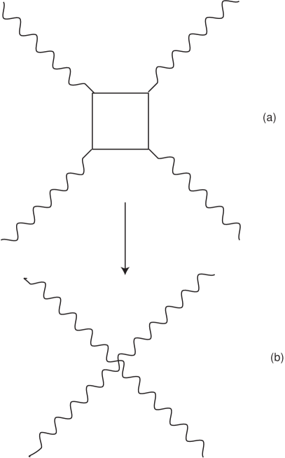
Figure 1: QED photon-photon (logarithmic divergent) scattering diagram in (a). The Euler-Heisenberg effective interaction in (b).

Let us suppose to be interested in understanding how the cross section for the photon-photon scattering scales with the energy of the photon in the limit in which this is lower than the rest energy of the electron. From an effective field theory point of view, this means that we are interested in building an effective theory in which the electron is excluded by the particle spectrum. The electron mass acts as the cutoff $\Lambda=m_{e}$ discussed before.

We therefore only need an interaction Lagrangian containing four photon fields. The symmetry principles instructing us about how to build this low energy effective theory are: Lorentz invariance, gauge invariance and the ${\cal P,C,T}$ symmetries. To the lowest order we can therefore write the so called Euler-Heisenberg Lagrangian:

$${\cal L}_{\rm eff}=\frac{\alpha^{2}}{m_{e}^{4}}\left[a_{1}(F_{\mu\nu}F^{\mu\nu})^{2}+a_{2}(F_{\mu\nu}{\tilde{F}}^{\mu\nu})^{2}\right]+O(1/m_{e}^{8}),$$ (1)

written in such a way to have the correct mass dimension. $a_{1,2}$ are the constants multiplying respectively the scalar squared and the pseudoscalar squared terms. The presence of $F_{\mu\nu}{\tilde{F}}^{\mu\nu}$ explains why we cannot have odd powers in higher order terms. Every gradient of the photon field, in the lowest order Euler-Heisenberg Lagrangian, produces a factor of $E_{\gamma}$. We can therefore argue that the cross section scales as:

$$\sigma\propto\left(\frac{\alpha^{2}E_{\gamma}^{4}}{m_{e}^{4}}\right)^{2}\frac{1}{E_{\gamma}^{2}},$$ (2)

i.e., $\sigma\propto\frac{E_{\gamma}^{6}}{m_{e}^{8}}$. The phase space factor $\frac{1}{E_{\gamma}^{2}}$ is needed because $\sigma$ has dimensions of a surface and $E_{\gamma}$ is the only dimensional parameter in the effective theory. The effective approach description is the one given in fig. 1(b). Anyway we could calculate the photon-photon scattering in QED, see fig. 1(a), by the virtual electron box (we should add five more diagrams renormalizing its logarithmic divergence), i.e., we could calculate the $\sigma$ of the process at high energy using the fundamental theory and then consider the low energy limit of the result. In such a way, through the matching of high and low energy Green’s functions, we could obtain the constants $a_{1}$ and $a_{2}$. If we didn’t knew QED, we should have fixed $a_{1}$ and $a_{2}$ by matching with the experiment. In the case of effective hadron Lagrangians, this is the problem: one cannot calculate the couplings (like $a_{1}$ and $a_{2}$), essential for the phenomenological predictions, by a matching with QCD. This is why one tries to build effective models, intermediate in energy between QCD and the hadron world, that could allow this matching.

2.2 Heavy quark effective theory

The physics we are interested in, is that of mesons containing one heavy quark ($b$ or $c$) [16]-[22]. These states present a large separation of energy scales: on one hand we have the heavy quark mass $m_{Q}$ and, on the other hand, we have $\Lambda_{\rm QCD}$, the asymptotic freedom scale, which limits the boundary between the strong coupling and the weak coupling region. The heavy quark is surrounded by a cloud of light quark states interacting with it through soft gluons having momenta of order $\Lambda_{\rm QCD}\simeq 200-300$ MeV. Being $m_{Q}>>\Lambda_{\rm QCD}$, we understand that the exchanged soft gluons can resolve only larger distances than the heavy quark Compton wavelenght. This means that light quark degrees of freedom are blind to the heavy quark flavor (i.e., to mass) and spin. For the light degrees of freedom, the heavy quark is simply a static chromoelectric source as the proton is simply a source of Coulombic potential for the electron in the hydrogen atom (chromomagnetic effects are suppressed by a factor of $1/m_{Q}$; spin-spin coupling terms between light and heavy degrees of freedom are also $1/m_{Q}$ terms).

We can therefore state that light degrees of freedom in an heavy meson have a new symmetry property, not remnant of the underlying QCD description, with respect to flavor and spin rotations of the heavy quark with which they interact. In particular, the excitation spectra of two heavy mesons containing two different heavy quarks $Q_{1}$ and $Q_{2}$ with $m_{Q_{1}},m_{Q_{2}}>>\Lambda_{\rm QCD}$, are the same once one overlaps the ground states. Due to flavor symmetry, it happens something like the atomic physics independence of the electron structure on the neutron number contained in the nucleus. Due to spin symmetry, each excitation level will be a doublet, degenerate in the total spin (if light degrees of freedom are not carrying zero spin).

In a seminal paper by H. Georgi [23], the initial ideas on heavy mesons and flavor-spin symmetries [24, 25] are translated in the effective field theory language. The aim is that of building a low energy theory where the heavy quark mass is considered infinite, $m_{Q}\to\infty$, since it is greater than all other energy scales appearing in the effective theory, while the heavy quark velocity, which is practically the same of that of the entire hadron, is a conserved contant of motion. Consider:

$$P^{\mu}=m_{H}v^{\mu},$$ (3)

the momentum of a meson having mass $m_{H}$ and containing an heavy quark of mass $m_{Q}$. In the $m_{Q}\to\infty$ limit, $m_{H}=m_{Q}$. Of course, in physical situations, the infinite mass limit is not rigorously fulfilled and $m_{H}\neq m_{Q}$. If we suppose that the light degrees of freedom carry a small momentum $q^{\mu}$, we can define the heavy quark momentum as:

$$p^{\mu}=P^{\mu}-q^{\mu}=m_{Q}v^{\mu}+k^{\mu},$$ (4)

where the “residual” momentum $k^{\mu}$ is defined as follows:

$$k^{\mu}=(m_{H}-m_{Q})v^{\mu}-q^{\mu}.$$ (5)

Let us now consider the hadron scattering from an external potential. After the interaction we have a new hadron state, containing the same heavy quark, and carrying momentum:

$$P^{\mu}=m_{Q}v^{\prime\mu}+s^{\mu},$$ (6)

where $s^{\mu}$ is the finite momentum exchanged with the external potential in the $m_{Q}\to\infty$ limit. If $s^{\mu}$ is a finite amount of momentum, then $v^{\mu}=v^{\prime\mu}$ (a finite momentum exchange cannot produce an infinite hadron momentum difference). This means that the velocity is a conserved constant of motion, i.e., it isn’t any more a dynamical degree of freedom.

When the heavy quark interacts with light degrees of freedom, only fluctuations of the residual momentum (of order $\Lambda_{\rm QCD}$) have to be considered, while variations of velocity are certainly excluded. QCD interactions do not vary $v$; only weak (or electromagnetic) interactions can annihilate the heavy quark and create a new one that can be different in flavor, spin and velocity.

In the Georgi’s paper it is therefore introduced a superselection rule for the velocity of an heavy quark: the fields describing the heavy quark in the effective theory should be $h_{v}(x)$ fields, i.e., depending on $x$ and $v$. For different $v$’s we have different heavy quark fields.

We have discussed the flavor-spin symmetry adopting the hypothesis of an heavy quark at rest. But now we can observe that the flavor-spin symmetry connects two heavy hadrons containing different heavy quark flavors only if they have the same velocity. In other words the $SU(2N_{h})$ flavor-spin symmetry, where $N_{h}$ is the number of heavy flavors, transforms meson states $M_{Q_{i}}$ in meson states $M_{Q_{j}}$, having different $i\neq j$ flavors, provided that $Q_{i}$ and $Q_{j}$ have the same velocity (not the same momentum: therefore flavor-spin symmetry is a symmetry of certain matrix elements, not an S-Matrix symmetry).

Importantly, flavor-spin symmetry is not an exact symmetry since the heavy masses aren’t infinite: the technology allowing to compute the $1/m_{Q}$ corrections is the HQET (Heavy-Quark-Effective-Theory).

In this paper we will make frequent use of the heavy quark effective propagator. This is derived by the QCD fermion propagator adopting the momentum formula introduced above:

$$p^{\mu}_{Q}=m_{Q}v^{\mu}+k^{\mu}.$$ (7)

In the $m_{Q}\to\infty$ limit, the propagator:

$$i\frac{\gamma\cdot p_{Q}+m_{Q}}{p_{Q}^{2}-m_{Q}^{2}},$$ (8)

becomes:

$$\frac{1+\gamma\cdot v}{2}\frac{i}{v\cdot k},$$ (9)

where we have used the relation $k\simeq\Lambda_{\rm QCD}$. The vertex describing the heavy quark-gluon interaction in QCD is:

$$-ig\gamma_{\mu}T^{a},$$ (10)

where $T^{a}$ is a generator of $SU(3)_{c}$ and $g$ is the coupling constant of strong interactions. Due to the structure of the propagator, the vertex is always intermediate between the $\frac{1+\gamma\cdot v}{2}$ projectors and therefore the vertex in the effective theory is:

$$-ig\frac{1+\gamma\cdot v}{2}\gamma_{\mu}\frac{1+\gamma\cdot v}{2}T^{a}=-igv_{\mu}T^{a}\frac{1+\gamma\cdot v}{2}.$$ (11)

The $\frac{1+\gamma\cdot v}{2}$ projectors, that appear in propagators and vertices, can be brought on the external lines of Feynman graphs, where they are annihilated by the on shell heavy quark spinors $h_{v}$ having the property that $\gamma\cdot vh_{v}=h_{v}$, see 2.2.1. We have therefore obtained the following two Feynman rules:

$${\rm propagator} = \frac{i}{v\cdot k}$$ (12)

$${\rm vertex} = -igv^{\mu}T^{a}.$$ (13)

Since here the heavy quark mass is absent, the flavor symmetry is manifested. Moreover there are no Dirac matrices, therefore also the spin symmetry is manifested.

2.2.1 $1/m_{Q}$ expansion

The Feynman rules given above can be considered as the basic definitions of the heavy quark effective theory. The same results can also be obtained using a field theoretical approach [23] avoiding the use of QCD Feynman rules like the propagator expression (8). Among effective theories, HQET has a particular role: one of the main goals of HQET is that of describing the properties of heavy hadron decays, therefore, even if there is the large separation of scales above mentioned, we cannot remove completely the heavy quark state from the low energy effective theory, see section 2.1. What can instead be eliminated in the effective theory, are the components of the heavy quark spinor describing its fluctuation around the mass shell since, in the $m_{Q}\to\infty$ limit, the heavy quark is almost on shell and carries almost the entire hadron momentum. It is therefore useful to decompose the heavy quark QCD spinor, $Q(x)$, in its small and large components:

$$Q(x)=e^{-im_{Q}v\cdot x}(H_{v}(x)+h_{v}(x)),$$ (14)

where:

$$H_{v}(x) = e^{im_{Q}v\cdot x}\frac{1+\gamma\cdot v}{2}Q(x)$$ (15)

$$h_{v}(x) = e^{im_{Q}v\cdot x}\frac{1-\gamma\cdot v}{2}Q(x).$$ (16)

Two properties are evident: $\gamma\cdot vh_{v}=h_{v}$ and $\gamma\cdot vH_{v}=-H_{v}$. Moreover, reminding the $\gamma_{0}$ structure, one can see that in the rest frame, $v=(1,0,0,0)$, $h_{v}$ corresponds to the upper components, the so called large components of the quadrispinor $Q$, while $H_{v}$ correspond to its inferior components, the so called small ones. $h_{v}$ annihilates an heavy quark having velocity $v$, $H_{v}$ creates an heavy antiquark having velocity $v$. Let’s consider the following virtual process discussed by Neubert [16]: an heavy quark propagating forward in time, at the event $a$ inverts his way in the opposite temporal direction and from the $b$ event on, it propagates again forward in time. In $a$ we have the annihilation of a virtual heavy quark-antiquark pair and in $b$ the creation. The energy in the intermediate virtual state, the one propagating between $a$ and $b$, is certainly larger, with respect to the initial one, of about $2m_{Q}$.

Therefore, this intermediate state can only propagate over distances of order $1/2m_{Q}$, which are very short if compared with the typical hadron physics distances, of order $1/\Lambda_{\rm QCD}$. The intermediate virtual state, that is evidently connected to the action of $H_{v}$ in $b$, can be simply substituted by the propagator $1/2m_{Q}$. We can therefore state that there is no sufficient energy to create a virtual heavy quark-antiquark pair in HQET or, in other words, this process is suppressed at order $1/m_{Q}$. We must therefore proceed to the systematic elimination of the $H_{v}$ field from the effective Lagrangian therefore obtaining a non-local effective action for $h_{v}$. This can be expanded in a $1/m_{Q}$ series of local operators.

In terms of $h$ and $H$, the QCD Lagrangian for heavy quarks takes the form [16]:

$${\cal L}_{\rm QCD} = \bar{Q}(i\gamma\cdot D-m_{Q})Q$$ (17)

$$= \bar{h}_{v}(iv\cdot D)h_{v}-\bar{H}_{v}(iv\cdot D+2m_{Q})H_{v}$$

$$+ \bar{h}_{v}(i\gamma\cdot\tilde{D})H_{v}+\bar{H}_{v}(i\gamma\cdot\tilde{D})h_{v},$$

where:

$$\tilde{D}^{\mu}=D^{\mu}-v^{\mu}v\cdot D.$$ (18)

We conclude that $h$ describes massless light degrees of freedom, while $H$ describes fluctuations having a mass of $2m_{Q}$. The latter must be eliminated from the effective theory. From the last two terms in ${\cal L}_{\rm QCD}$, describing the creation (annihilation) of quark-antiquark pairs, we can see that $H$ and $h$ fields are mixed together. If we compute the functional derivative of ${\cal L}_{\rm QCD}$ with respect to $\bar{H}$, we obtain the following equation of motion for $H$:

$$(iv\cdot D+2m_{Q})H_{v}=i\gamma\cdot\tilde{D}h_{v},$$ (19)

that can be formally solved for $H_{v}$ and the resulting expression can be inserted in ${\cal L}_{\rm QCD}$, giving:

$${\cal L}_{\rm eff}=\bar{h}_{v}(iv\cdot D)h_{v}+\bar{h}_{v}(i\gamma\cdot\tilde{D}\frac{1}{2m_{Q}+iv\cdot D}i\gamma\cdot\tilde{D})h_{v},$$ (20)

where the second term describes the virtual process discussed above. In the momentum space, derivatives acting on $h$ fields correspond to powers of the residual momentum $k$, therefore we can perform the following power expansion:

$${\cal L}_{\rm eff}=\bar{h}_{v}(iv\cdot D)h_{v}+\frac{1}{2m_{Q}}\sum_{n=0}^{\infty}\bar{h}_{v}i\gamma\cdot\tilde{D}\left(-\frac{iv\cdot D}{2m_{Q}}\right)^{n}i\gamma\cdot\tilde{D}h_{v}.$$ (21)

It is not difficult to prove the following identity:

$$\frac{1+\gamma\cdot v}{2}(i\gamma\cdot\tilde{D})^{2}\frac{1+\gamma\cdot v}{2}=\frac{1+\gamma\cdot v}{2}\left[(i\tilde{D})^{2}+\frac{g}{2}\sigma_{\mu\nu}G^{\mu\nu}\right]\frac{1+\gamma\cdot v}{2},$$ (22)

where $G_{\mu\nu}$ is the gluon strenght tensor field and the well known property $[iD_{\mu},iD_{\nu}]=igG_{\mu\nu}$ holds [26]. Considering the $n=0$ term in the expansion (21), one finds the interesting result:

$${\cal L}_{\rm eff}=\bar{h}_{v}(iv\cdot D)h_{v}+\frac{1}{2m_{Q}}\bar{h}_{v}(i\tilde{D})^{2}h_{v}+\frac{g}{4m_{Q}}\bar{h}_{v}\sigma_{\mu\nu}G^{\mu\nu}h_{v}+O(1/m_{Q}^{2}).$$ (23)

The $m_{Q}\to\infty$ limit selects only the first term in the preceding Lagrangian. Since the heavy quark mass is large, but not infinite, all other terms are to be considered as corrections, that, as we can see, are included in the effective theory in a systematic way. The first term in ${\cal L}_{\rm eff}$ allows to write down the Feynman rules for propagator and gluon vertex already discussed before. Let us rewrite it including a sum over $N_{h}$ heavy flavors and a sum over velocities:

$${\cal L}_{\rm eff}^{(1)}=\sum_{i=1}^{N_{h}}\int d^{3}{\bf v}\frac{1}{2v_{0}}\bar{h}_{v}^{(i)}(iv\cdot D)h_{v}^{(i)}.$$ (24)

Since in this Lagrangian there aren’t terms containing $m_{Q}$, we can deduce that ${\cal L}_{\rm eff}^{(1)}$ is invariant under flavor space rotations. Moreover, since no Dirac’s $\gamma$ are present, the interactions among heavy quarks and gluons conserve heavy quark spins. This is the $SU(2N_{h})$ symmetry already discussed. To be rigorous, since Lorentz transformation can boost the heavy quark velocity, the symmetry group should be ${\rm Lorentz}\times SU(2N_{h})^{\infty}$.

Let’s now consider the two operators of order $1/m_{Q}$ in (24). To understand their role it is convenient to write them in the rest frame of the heavy quark $v=(1,0,0,0)$:

$$\frac{1}{2m_{Q}}\bar{h}_{v}(i\tilde{D})^{2}h_{v} \rightarrow -\frac{1}{2m_{Q}}\bar{h}_{v}(i{\bf D})^{2}h_{v}$$ (25)

$$\frac{g}{4m_{Q}}\bar{h}_{v}\sigma_{\mu\nu}G^{\mu\nu}h_{v} \rightarrow -\frac{g}{m_{Q}}\bar{h}_{v}({\bf S}\cdot{\bf H}_{c})h_{v},$$ (26)

where ${\bf H}_{c}^{i}=-\frac{1}{2}\epsilon^{ijk}G^{jk}$ and ${\bf S}$ is a spin operator defined as a $4\times 4$ matrix with Puli matrices $\frac{\sigma_{i}}{2}$ on the diagonal. Therefore the first operator is a kinetic energy operator connected to the residual motion of the off-mass-shell heavy quark. The second operator is the non Abelian extension of the Pauli interaction describing the chromomagnetic heavy quark spin coupling with the gluon field. We find confirmation that the heavy quark spin is decoupled by a factor of $1/m_{Q}$.

2.2.2 Relations with QCD

To match HQET with QCD at high energy, one must include some corrective effects in HQET due to high energy virtual processes. For example, the weak current transforming the flavor from $b$ to $c$ must be corrected at the $\alpha_{s}$ order both in QCD and in HQET. We can expect that there are differences between these corrections. These differences instruct on how one should modify the coefficient of the weak current in HQET and on what terms should be added to the HQET current to guarantee the correct matching between the low energy and the fundamental theory. Let us consider for example the case of the current $\bar{b}\gamma^{\mu}c$. The $\gamma^{\mu}$ of QCD has to be substituted by the $\Gamma^{\mu}$ of HQET where [27]:

$$\Gamma^{\mu}=\left(1+C_{0}\frac{\alpha_{s}}{\pi}\right)\gamma^{\mu}+\frac{\alpha_{s}}{\pi}\sum_{i}C_{i}\Gamma_{i}^{\mu},$$ (27)

and $\Gamma_{i}^{\mu}$ are new structures containing $v$ and $v^{\prime}$, i.e., the velocities of the heavy quark before and after the weak interaction vertex. In practice, this type of calculation is made by comparing the vertex diagrams where the fermionic heavy quark current is coupled to the weak current, up to order $\alpha_{s}$. We have therefore to compare four QCD diagrams with four HQET diagrams. The difference between the two set of diagrams lays in the Feynman rules describing the strong vertices and the heavy quark propagators. The first of the mentioned four diagrams is the three level diagram (the simple tree weak vertex). In the remaining three diagrams, one should close the gluon line on the heavy quark line according to the three diagrammatically possible ways.

2.3 Chiral lagrangians

The QCD Lagrangian with three massless quark flavors incorporates the $U(3)_{L}\times U(3)_{R}$ global symmetry [28]. The left- and right- handed components $q_{L}=(u_{L},d_{L},s_{L})$ and $q_{R}=(u_{R},d_{R},s_{R})$ transform respectively as the fundamental representations of $U(3)_{L}$ and $U(3)_{R}$ respectively. Anyway, the symmetry group of the quantum theory is a subgroup of $U(3)_{L}\times U(3)_{R}$, this is what is usually called anomalous breaking at the quantum level of a symmetry of the classical Lagrangian. The reason for this phenomenon is that $U(1)_{A}$ is not a good symmetry of the theory since its generator, $Q_{5}$, is not a time independent quantity due to the presence of instantonic configurations of gauge fields in Yang-Mills theories. The quantum theory has therefore the following symmetry group: $SU(3)_{L}\times SU(3)_{R}\times U(1)_{V}$, the chiral symmetry. Anyway the physical states are invariant only under $SU(3)_{V}\times U(1)_{V}$; for example the baryon spectrum is not doubled in two spectra having opposite parity, but it is well described as an octet representation of $SU(3)_{V}$ having baryon number $1$: this is the phenomenon of spontaneous symmetry breaking. The mechanism underlying the spontaneous symmetry breaking of chiral symmetry is most likely of non perturbative nature. The energy scale associated to this phenomenon is $\Lambda_{\chi}\simeq 1$ GeV (this point will be discussed with greater detail later).

Each broken global symmetry implies the exitence of a Nambu-Goldstone (NG) boson emerging as a scalar massless particle induced by the non symmetric structure of theory’s vacua. The chiral symmetry is not an exact symmetry because light quark masses are not exactly zero: they are simply small if compared with $\Lambda_{\rm QCD}$. Therfore we should expect to have pseudo-NG-bosons having small masses.

Light quark masses are slightly dissimilar to each other causing that NG bosons will also have slightly dissimilar masses. On the other hand, since light quark masses are much smaller than $\Lambda_{\rm QCD}$, the light baryons are almost all degenerate in mass (because, differently from NG bosons, sending to zero the light quark masses, baryon masses should tend to a value different from zero).

Due to the lightness of pseudo NG bosons, it emerges a hierarchy of energy scales allowing to decide that NG bosons interactions at energies much lower than $\Lambda_{\chi}$ can be described within a chiral effective theory. Even if in this case the separation among energy scales is not as large as in the case of heavy quark effective theory, the chiral effective theory, developed in seminal papers by Weinberg [14], Manohar and Georgi [29] and by Gasser and Leutwyler [30], is a great success.

Since chiral symmetry is spontaneously broken, we have a chiral condensate different from zero that we can write as [31]:

$$\langle\bar{\psi}_{jR}\bar{\psi}_{iL}\rangle=c\Sigma{ij},$$ (28)

where $c$ is the value of the condensate, while $\Sigma$ defines a direction of the condensate in the flavor space. All $\Sigma$’s orientations are degenerate vacua that are mapped one in the other through the $SU(3)_{L}\times SU(3)_{R}$ transformations:

$$\Sigma\rightarrow L\Sigma R^{+}.$$ (29)

$\Sigma$ is normalized in such a way that $\Sigma^{+}\Sigma=1$.

When $\Sigma$ has a spatial dependency, then we are dealing with a Goldstone excitation: low energy excitation are in fact characterized by a vacuum configuration that varies from point to point in the space, being the orientation of the vacuum state a function having a smooth dependence on the position (think of spin waves in a ferromagnet). The excitation energy is as small as one likes when one considers very small $\Sigma(x)$ variations over large lenght scales: this is the case of NG bosons.

In order to construct a chiral effective theory, one needs to follow the instructions that we have already described for a general effective theory. One must write the most general Lagrangian, containing the $\Sigma$ field, consistent with relativistic invariance, ${\cal PCT}$, QCD chiral symmetry.

In the chiral effective Lagrangian there aren’t terms not containing derivatives [13]. If there was such a term, it could only be constant (think of ${\rm Tr}[\Sigma^{+}\Sigma]$ where $\Sigma^{+}\Sigma=1$). Every invariant function of $\Sigma$ without derivatives, is just a constant. If we don’t exclude terms not containing derivatives, we could have a Lagrangian containing only zero momentum $\Sigma$ fields. But a NG boson with zero momentum simply does not exist, it is equivalent to the vacuum.

The first non trivial term that we are going to consider in the chiral Lagrangian construction is the one having two derivatives:

$${\cal L}_{2}=\frac{f_{\pi}^{2}}{4}{\rm Tr}[\partial_{\mu}\Sigma\partial^{\mu}\Sigma^{+}],$$ (30)

this is the only allowed one with two derivatives. $f_{\pi}$ is the pion decay constant, i.e., one of the energy scales characterizing the pion (the other one is its mass). The $\Sigma$ field is described as the exponential of NG boson fields:

$$\Sigma(x)=e^{\frac{2\pi(x)i}{f_{\pi}}},$$ (31)

where:

$$\pi(x)=\pi^{a}(x)T^{a},$$ (32)

$T^{a}$ being the $8$ generators of $SU(3)$-colour. Such an expression for the $\Sigma$ field amounts to consider the NG fields as the angular variables describing the vacuum rotations. Moreover let’s observe that under the transformation (29), the $\pi$ fields transform non linearly as complicated functions of $L$ and $R$. The exponential representation (31), is only a particular one, the simplest, among all the possible non linear representations of $\pi$ fields. All of those give the same S-matrix [32].

Let us now take the first term introduced in (30). This can be expanded in powers of the pion momentum in the following way:

$${\cal L}_{2}={\rm Tr}[\partial_{\mu}\pi\partial^{\mu}\pi]+\frac{1}{2f_{\pi}^{2}}{\rm Tr}[[\pi,\partial_{\mu}\pi]^{2}]+.....,$$ (33)

where higher order terms give non-linear interactions with NG bosons. Besides ${\cal L}_{2}$ we can introduce higher dimensional operators ${\cal L}_{n}$, i.e., containing a larger number of derivatives. Manohar and Georgi have shown that the energy scale $\Lambda$ controlling this expansion in an increasing number of derivatives $\frac{\partial}{\Lambda}$ is $\Lambda=\Lambda_{\chi}$ and they estimate $\Lambda_{\chi}\simeq 4\pi f_{\pi}\simeq 1$ GeV. This limits the range of validity of the Lagrangian to the low energy domain since the pion momenta have to be small compared to $\Lambda_{\chi}$ (otherwise the derivative expansion gets divergent very soon). We will make these points clear in the next sub-session.

2.3.1 $\Lambda_{\chi}$

As stated above, besides (30), the chiral effective Lagrangian may also contain terms with an higher number of derivatives. Let’s consider ${\cal L}_{4}$ containing four derivatives, i.e., proportional to:

$${\cal L}_{4}\simeq{\rm Tr}[\partial_{\mu}\Sigma\partial_{\nu}\Sigma^{+}\partial^{\mu}\Sigma\partial^{\nu}\Sigma^{+}].$$ (34)

An higher number of derivatives means an higher number of pion momenta. As already stressed, in a low energy effective theory a term such as ${\cal L}_{4}$ needs to be multiplied by some inverse power of $\Lambda$, an energy scale characterizing the upper energy bound of the effective theory and representing the parameter that controls the convergence of the pion momentum expansion. This $\Lambda$ can be associated to the energy scale of spontaneous chiral symmetry breaking, $\Lambda_{\chi}=\Lambda$, and this association will allow for an estimation of $\Lambda_{\chi}$ that is going to be used throughout this work. We will follow an argument due to Manohar and Georgi [29]. We can normalize ${\cal L}_{4}$ relatively to the lowest order term (30), adding two $\Lambda_{\chi}^{-1}$ powers for each additional derivative. The term having the correct mass dimension is:

$${\cal L}_{4}=\frac{f_{\pi}^{2}}{\Lambda_{\chi}^{2}}{\rm Tr}[\partial_{\mu}\Sigma\partial_{\nu}\Sigma^{+}\partial^{\mu}\Sigma\partial^{\nu}\Sigma^{+}].$$ (35)

If $\Lambda_{\chi}$ was much higher than pseudoscalar masses, then all orders having an higher number of derivatives with respect to (30) would be negligible. But we cannot formulate this hypothesis since radiative corrections to (30) produce a term as (35) and also higher order terms having an infinite coefficient. Thus, even if these terms are absent or negligible for a certain choice of the renormalization scale, they can be present and important for a different one. On the other hand, one could reasonably think that the $f_{\pi}^{2}/\Lambda_{\chi}^{2}$ coefficient should be numerically larger or equal to the variation induced in it by an $O(1)$ shift in the renormalization scale of radiative corrections to (30).

These considerations get particularly clear if one examines the $\pi-\pi$ scattering process. If we refer back to (30), we see that each four pion vertex has the following structure:

$$\frac{p^{2}\pi^{4}}{f_{\pi}^{2}}.$$ (36)

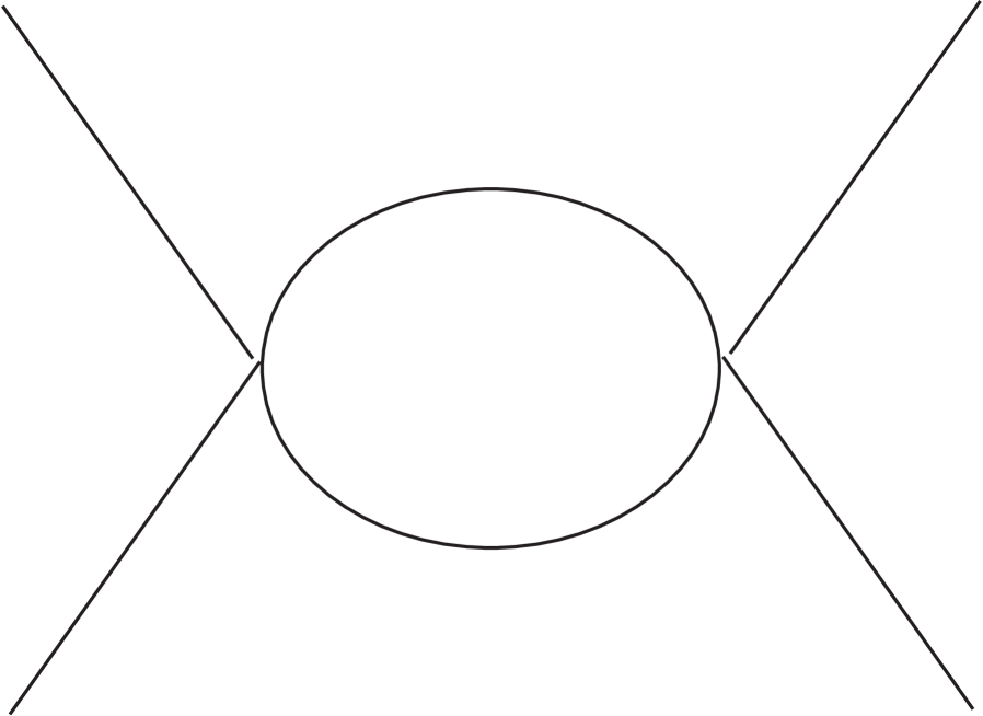
Figure 2: One loop diagram for $\pi-\pi$ scattering.

Using two of these four pion vertices to generate the one-loop diagram shown in fig. 2, we can obtain the particular case of pion-pion scattering diagram with all derivatives acting on the external legs (the same diagram in fig. 2 may have only two derivatives acting on external legs, while the two remaining could act on the internal ones. In such a situation we are facing a quadratically divergent diagram).

If instead one refers directly to (35), the fundamental four pion vertex has the form:

$$\frac{p^{4}\pi^{4}}{f_{\pi}^{2}\Lambda_{\chi}^{2}},$$ (37)

therefore one can also write the pion-pion scattering diagram with all derivatives acting on the external legs simply using the tree level diagram extracted from ${\cal L}_{4}$. The diagram in fig. 2, generated by two insertions of ${\cal L}_{2}$, is just a one-loop correction to the tree level process described by a single insertion of ${\cal L}_{4}$. The diagram in fig. 2 clearly gives:

$$\frac{p^{4}\pi^{4}}{f_{\pi}^{4}}\frac{1}{(2\pi)^{4}}\int_{\ell}\frac{1}{(\ell^{2})^{2}}=\frac{p^{4}\pi^{4}}{f_{\pi}^{4}}\frac{1}{(4\pi)^{2}}{\rm ln}\left(\frac{\Lambda_{\rm co}}{\mu}\right),$$ (38)

dividing by the correct symmetry factor and introducing a cutoff $\Lambda_{\rm co}$ and the renormalization scale $\mu$. To be consistent with a chiral effective theory scheme, we should limit the momenta circulating in the loop to $\Lambda_{\rm co}\simeq\Lambda_{\chi}$. Let’s now rescale $\mu$ in (38), of an $O(1)$ quantity: let’s take the Neper number. We obtain a variation of (38) amounting to:

$$\frac{1}{(4\pi)^{2}}\frac{p^{4}\pi^{4}}{f_{\pi}^{4}}.$$ (39)

The shift in the renormalization point $\mu$ can be absorbed into a redefinition of the coefficient $f_{\pi}^{2}/\Lambda_{\chi}^{2}$ in (35) and we have that (39) corresponds to a change in that coefficient amounting to:

$$\frac{1}{(4\pi)^{2}}.$$ (40)

But, as above observed, we can expect that:

$$\frac{f_{\pi}^{2}}{\Lambda_{\chi}^{2}}\geq\frac{1}{(4\pi)^{2}},$$ (41)

therefore:

$$\Lambda_{\chi}\leq 4\pi f_{\pi},$$ (42)

which suggest to use, as an estimate of the energy scale associated to spontaneous chiral symmetry breaking, the following one:

$$\Lambda_{\chi}=4\pi f_{\pi}\simeq 1{\rm GeV}.$$ (43)

In this work we will make use of a cutoff value close to $\Lambda_{\chi}$ for the same physical motivations here described. The fact that $f_{\pi}$ is a measure of the strength of the symmetry breaking is also discussed in [33].

2.3.2 The Manohar-Georgi Lagrangian

The effective Lagrangian defined below the chiral symmetry breaking scale contains, besides pion fields, also light quarks and gluons. Let’s define the $\xi$ field in the following way:

$$\xi=e^{i\frac{\pi}{f_{\pi}}},$$ (44)

i.e., $\xi=\sqrt{\Sigma}$. We know that under $SU(3)\times SU(3)$ transformations of the $\Sigma$ field, the NG bosons, represented by the $\pi$ matrix, undergo a non-linear transformation where $\pi_{a}\to\pi_{a}^{\prime}$, $\pi_{a}^{\prime}$ being non-linear functions of $\pi$, $L$, and $R$. The transformation properties of $\pi$ fields determine also the transformation properties under $SU(3)\times SU(3)$ of the $\xi$-fields. Since $\Sigma=\xi^{2}$:

$$\xi\to\xi^{\prime}=L\xi U^{+}=U\xi R^{+},$$ (45)

where $U$ is a non linear function of $L$, $R$ and $\pi$ that can be written as an ordinary $SU(3)$ matrix in the following way:

$$U=e^{iv},$$ (46)

and the Hermitian matrix $v$ contains “non-linearly” the $SU(3)\times SU(3)$ symmetry. The $U$ matrix is invariant under parity transformations exchanging $L$ with $R$ and $\pi$ with $-\pi$. If $L=R$, the chiral transformation reduces to a simple $SU(3)$ transformation and $U=L=R$. Through $\xi$ matrices we can construct two auxiliary fields:

$${\cal V}^{\mu} = \frac{1}{2}(\xi^{+}\partial^{\mu}\xi+\xi\partial^{\mu}\xi^{+})=\frac{1}{f_{\pi}^{2}}[\pi,\partial_{\mu}\pi]+.....$$ (47)

$${\cal A}^{\mu} = -\frac{i}{2}(\xi^{+}\partial^{\mu}\xi-\xi\partial^{\mu}\xi^{+})=\frac{1}{f_{\pi}}\partial_{\mu}\pi+.....,$$ (48)

which, under chiral transformation, behave like this:

$${\cal V}^{\mu} \to U{\cal V}^{\mu}U^{+}+U\partial^{\mu}U^{+}$$ (49)

$${\cal A}^{\mu} \to U{\cal A}^{\mu}U^{+}.$$ (50)

In particular, due to the transformation property of ${\cal V}^{\mu}$, we can treat it as a gauge field in a covariant derivative:

$$D^{\mu}=\partial^{\mu}+{\cal V}^{\mu}.$$ (51)

Let us now form the Lagrangian terms related to $u$, $d$ and $s$ quarks considered together in a unique triplet $\psi$ of flavor-$SU(3)$. $\psi$ is supposed to transform under $SU(3)\times SU(3)$ in the following way:

$$\psi\to U\psi.$$ (52)

The only term without derivatives is:

$$-m\bar{\psi}\psi,$$ (53)

where $m$ is not the current mass of the QCD Lagrangian. $m$ is a constituent mass whose origin can be related to the spontaneous breaking of chiral symmetry (we will come back on this point when we will introduce the constituent light quark mass in the CQM model).

We also have two derivative terms. The first one is the kinetic term:

$$i\bar{\psi}\gamma\cdot D\psi,$$ (54)

the other one is the interaction term between the light quarks and the pion. We will use the PCAC language [34] to introduce this term.

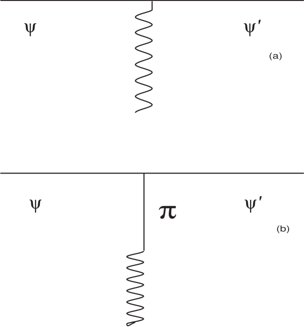
Figure 3: (b) represents the pion pole contribution to the diagram in (a).

The derivative operator of the axial current, $\partial A$, is a pseudoscalar operator with odd G-parity, isospin one and hypercharge zero. It has therefore all quantum numbers of the $i$-component of pion triplet. Let us consider the matrix element:

$$\langle\psi^{\prime}|\partial A|\psi\rangle,$$ (55)

where $\psi$ is a light quark field, see fig. 3(a). Many diagrams contribute to diagram in fig. 3(a); we choose that in fig. 3(b). This is equivalent to:

$$\langle\psi^{\prime}|\partial A|\psi\rangle=i\frac{\langle{\rm VAC}|\partial A|\pi\rangle\langle\pi\psi^{\prime}|\psi\rangle}{q^{2}-m_{\pi}^{2}}=i\frac{f_{\pi}m_{\pi}^{2}}{q^{2}-m_{\pi}^{2}}{\rm Amp}(\psi\to\psi^{\prime}\pi),$$ (56)

where ${\rm Amp}(\psi\to\psi^{\prime}\pi)$ denotes the amplitude for the process $\psi\to\psi^{\prime}\pi$ (the $i$ comes from the propagator). Clearly:

$${\rm Amp}(\psi\to\psi^{\prime}\pi)=\frac{q^{2}-m_{\pi}^{2}}{if_{\pi}m_{\pi}^{2}}\langle\psi^{\prime}|\partial A|\psi\rangle,$$ (57)

in the $q^{2}\to m_{\pi}^{2}$ limit. PCAC hypothesis consists essentially in defining the following off-mass-shell amplitude:

$$\widetilde{\rm Amp}(\psi\to\psi^{\prime}\pi)=\frac{q^{2}-m_{\pi}^{2}}{if_{\pi}q^{2}}\langle\psi^{\prime}|\partial A|\psi\rangle,$$ (58)

where $q$ is the pion momentum. At this point one must suppose that this off-mass shell amplitude varies smoothly within the $(0,m_{\pi}^{2})$ $q^{2}$-range. The chiral limit of $\widetilde{\rm Amp}$ is defined taking the $m_{\pi}\to 0$ limit and then the mass-shell-limit $q^{2}\to 0$ (the two procedures do not commute) hoping that the hypothesis on the smooth variability with respect to $q^{2}$ holds well (as is confirmed by the Goldberger-Treiman relation and by its physical consequences). The chiral off-mass shell amplitude is therefore:

$$\widetilde{\rm Amp}(\psi\to\psi^{\prime}\pi)\to-\frac{i}{f_{\pi}}\langle\psi^{\prime}|\partial A|\psi\rangle=\frac{q_{\mu}}{f_{\pi}}\langle\psi^{\prime}|A^{\mu}|\psi\rangle.$$ (59)

We can therefore have a Yukawa type coupling in the Lagrangian:

$$-\frac{i}{f_{\pi}}\bar{\psi}\gamma_{\mu}\gamma_{5}\psi q^{\mu}\pi,$$ (60)

and generalize it, see (48), in the following way:

$$\bar{\psi}\gamma\cdot{\cal A}\gamma_{5}\psi.$$ (61)

The Manhoar-Georgi Lagrangian to lowest oder, including also colour in the covariant derivative, is:

$${\cal L}_{\rm eff} = \bar{\psi}[\gamma\cdot(iD+{\cal V})]\psi+g_{A}\bar{\psi}\gamma\cdot{\cal A}\gamma_{5}\psi-m\bar{\psi}\psi$$ (62)

$$+ \frac{f_{\pi}^{2}}{4}{\rm Tr}[\partial^{\mu}\Sigma\partial_{\mu}\Sigma^{+}]-\frac{1}{2}{\rm Tr}[G_{\mu\nu}G^{\mu\nu}],$$

where $G_{\mu\nu}$ is the well known non-abelian strenght tensor of the gluon field $G_{\mu}=G_{\mu}^{a}T^{a}$. $g_{A}$ must be computed through a matching with QCD or extracted by a comparison with experimental data, or, as will be our case, with some more fundamental effective model.

2.3.3 Heavy mesons and chiral Lagrangians

We are going to discuss of an effective chiral Lagrangian describing the interaction of soft pions (and kaons) with mesons containing an heavy quark. As we saw in section 2.2, heavy meson fields should be described through the HQET formalism. In order to implement the flavor-spin symmetry, the field describing an heavy meson has to be independent on heavy quark mass and spin. On the contrary, it can be characterized by the total angular momentum $s_{\ell}$ of light degrees of freedom. To each $s_{\ell}$ value, there corresponds a doublet of states degenerate in mass with total angular momentum $J=s_{\ell}\pm\frac{1}{2}$. In correspondence of $s_{\ell}=\frac{1}{2}$, for example, we have the $P$ and $P^{*}$ mesons being respectively the pseudoscalar and vector components of the spin symmetry doublet. If the heavy quark is $c$, $P$ and $P^{*}$ correspond to $D$ and $D^{*}$, while if the heavy quark is $b$, they are the states $B$ and $B^{*}$ respectively.

Let us consider the negative parity doublet $(P,P^{*})$. We can associate a unique super-field $H$ [35] describing both states. This super-field must have two spinor indices: one connected to the heavy quark and the other to the light quark. The structure of $H$ is that of a $4\times 4$ Dirac matrix. If one performs a Lorentz transformation, $H$ behaves like:

$$H\to D(\Lambda)HD(\Lambda)^{-1},$$ (63)

where $\Lambda$ is the usual $4\times 4$ representation of the Lorentz group. An explicit matrix representation is the following:

$$H=\frac{1+\gamma\cdot v}{2}[P^{*}_{\mu}\gamma^{\mu}-P\gamma_{5}],$$ (64)

and we define:

$$\bar{H}=\gamma_{0}H^{\dagger}\gamma_{0}.$$ (65)

$v$ is the velocity of the heavy meson and the following transversality condition holds: $v^{\mu}P^{*}_{\mu}=0$ and $M_{H}=M_{P}=M_{P^{*}}$. We mention also the following useful relations: $\gamma\cdot vH=-H\gamma\cdot v$, $\bar{H}\gamma\cdot v=-\gamma\cdot v\bar{H}=\bar{H}$. $P$ and $P^{*\mu}$ are the annihilation operators normalized in the following way:

$$\langle{\rm VAC}|P|Q\bar{q}(0^{-})\rangle = \sqrt{M_{H}}$$ (66)

$$\langle{\rm VAC}|P^{*\mu}|Q\bar{q}(1^{-})\rangle = \epsilon^{\mu}\sqrt{M_{H}}.$$ (67)

The formalism apt to describe higher spin meson states and the effective Lagrangian terms associated to them, is extensively developed in [36]. We are interested in considering the $p$-wave ($\ell=1$) of the $Q\bar{q}$ system. HQET predicts the existence of two degenerate doublets: $(0^{+},1^{+})$ and $(1^{+},2^{+})$ for each heavy quark $c$ or $b$. The related superfields are:

$$S = \frac{1+\gamma\cdot v}{2}[P^{*\prime}_{1\mu}\gamma^{\mu}\gamma_{5}-P_{0}]$$ (68)

$$T^{\mu} = \frac{1+\gamma\cdot v}{2}\left[P^{*\mu\nu}_{2}\gamma_{\nu}-\sqrt{\frac{3}{2}}P^{*}_{1\nu}\gamma_{5}\left(g^{\mu\nu}-\frac{1}{3}\gamma^{\nu}(\gamma^{\mu}-v^{\mu})\right)\right].$$ (69)

These two doublets have respectively $s_{\ell}=\frac{1}{2}$ and $s_{\ell}=\frac{3}{2}$. This classification with respect to $s_{\ell}$ is the more reasonable one since we know that the dynamics is completely independent on the spin and on the mass of the heavy quark $Q$. Observe that in the limit of infinite heavy quark mass, $s_{\ell}$ and $s_{Q}$ are separately conserved. We can introduce the total spin ${\bf J}$, defined as the total angular momentum of the heavy and light quark in the rest frame of the heavy quark:

$${\bf J}={\bf s_{\ell}}+{\bf s}_{Q}.$$ (70)

Heavy mesons can interact with $\pi$ fields through their light degrees of freedom. The interaction terms of the NG boson octet with heavy meson fields must be written in an effective Lagrangian including the essential symmetry properties: chiral symmetry and heavy flavor-spin symmetry. This heavy-light chiral effective Lagrangian can be expanded with respect to:

• NG bosons momenta
  

• $\frac{1}{m_{Q}}$ powers

An heavy-light Lagrangian has been introduced almost simultaneously by different groups [37]:

$${\cal L}=\frac{f_{\pi}^{2}}{4}{\rm Tr}[\partial^{\mu}\Sigma\partial_{\mu}\Sigma^{+}]-{\rm Tr}[\bar{H}iv\cdot DH]+g{\rm Tr}[\bar{H}H\gamma\cdot{\cal A}\gamma_{5}]+.....,$$ (71)

where ellipses indicate the presence of an infinite number of operators having higher dimensionality, including those responsible for explicit chiral symmetry breaking, i.e., terms containing light hadron masses, and those of order $\Lambda_{\rm QCD}/m_{Q}$, violating the flavor-spin symmetry (such as the color magnetic moment operator). The covariant derivative has been defined in (51).

Let us consider for example the term having the factor of $g$ in eq. (71): it describes the coupling of $H$-type mesons with NG bosons, see eq. (48). We will come back on terms of this kind many times. Including also $S$ and $T$ mesons we have:

$${\cal L}=ig{\rm Tr}[\bar{H}H\gamma\cdot{\cal A}\gamma_{5}]+ig^{\prime}{\rm Tr}[\bar{S}S\gamma\cdot{\cal A}\gamma_{5}]+ig^{\prime\prime}{\rm Tr}[\bar{T}^{\mu}T_{\mu}\gamma\cdot{\cal A}\gamma_{5}].$$ (72)

At the lower order of the derivative expansion we can also write the interaction terms describing transitions between different doublets; for example:

$${\cal L}=if{\rm Tr}[\bar{S}T^{\mu}{\cal A}_{\mu}\gamma_{5}]+if^{\prime}{\rm Tr}[\bar{H}S\gamma\cdot{\cal A}\gamma_{5}]+h.c.$$ (73)

A particular case is that of transitions between $T$ and $H$ states. Let’s suppose to consider the following s-wave interaction Lagrangian:

$${\cal L}=ir{\rm Tr}[\bar{H}T^{\mu}{\cal A}_{\mu}\gamma_{5}].$$ (74)

We can therefore write the $S$-matrix element:

$$\langle{\rm out}D\pi|D_{2}{\rm in}\rangle,$$ (75)

as:

$$\langle D\pi|i{\cal L}|D_{2}\rangle = -r\langle D|P|{\rm VAC}\rangle\langle\pi|\frac{\partial_{\mu}\pi}{f_{\pi}}|{\rm VAC}\rangle\langle{\rm VAC}|P^{*\mu\nu}_{2}|D_{2}\rangle{\rm Tr}\left[\frac{1+\gamma\cdot v}{2}\gamma_{\nu}\right]$$ (76)

$$= ir\sqrt{m_{D}m_{D_{2}}}\frac{q_{\mu}}{f_{\pi}}2\epsilon^{\mu\nu}v_{\nu},$$ (77)

where the first order in the expansion (48) has been used. Due to transversality, this term is certainly zero, since $\epsilon^{\mu\nu}v_{\nu}=0$. Since the process we are discussing is entirely due to the strong interaction, the velocity conservation rule, introduced in 2.2, holds, i.e., the velocity of $D$ and $D_{2}$ are the same.

We conclude that the Lagrangian (74) cannot be the right one to describe the $T\to H\pi$ transition. We need one more Lorentz index coming from the insertion of another derivative under the trace sign. This derivative should be accompained with a negative power of $\Lambda_{\chi}$, giving the right mass dimension to the interaction term and controlling the expansion in NG bosons momenta.

The $d$-wave Lagrangian is:

$${\cal L}=\frac{h_{1}}{\Lambda_{\chi}}{\rm Tr}[\bar{H}T^{\mu}(iD_{\mu}\gamma\cdot{\cal A})\gamma_{5}]+\frac{h_{2}}{\Lambda_{\chi}}{\rm Tr}[\bar{H}T^{\mu}(i\gamma\cdot D{\cal A}_{\mu})\gamma_{5}]+{\rm h.c.}$$ (78)

With an analogous approach super-fields having higher spins may be constructed.

3 CQM

3.1 The CQM model

CQM is a Constituent-Quark-Meson-Model that has been introduced and discussed in a number of recent research papers [38, 39, 40, 41, 42]. The model, based on an effective Lagrangian describing quark-meson interactions, is relativistic, incorporates the flavor-spin symmetry in the heavy sector and the chiral symmetry in the light quark sector. In the following sections CQM will be reviewed in detail. Section 4.1 and subsequent sections are instead devoted to the CQM phenomenological applications to heavy meson physics.

In the well known old paper [43], Y. Nambu and G. Jona-Lasinio discuss the possibility that the nucleon mass can be due to an unknown primary interaction bounding hypothetical massless primary fermions. In their model, the same interaction bounds nucleon pairs giving rise to pions and the mass of the Dirac particle emerges as a result of the primary interaction in the same way as the energy gap in a BCS superconductor [44] is connected to the formation of correlated Cooper pairs of electrons, as a result of a phonon-mediated “primary” interaction (the finite energy that is needed to break a Cooper pair is proportional to the BCS gap).

The primary interaction in the Nambu-Jona-Lasinio model is a non linear four fermion interaction, already discussed in an older paper by Heisenberg et al.:

$$G[(\bar{\psi}\gamma_{\mu}\psi)^{2}-(\bar{\psi}\gamma_{\mu}\gamma_{5}\psi)^{2}].$$ (79)

In some recent papers [45, 46], the problem of the bosonization of a Nambu-Jona-Lasinio (NJL) like Lagrangian, where the fundamental fields are quarks, has been extensively studied. The aim is to derive an effective theory of mesons starting from a model (the NJL model) incorporating global chiral symmetry and its spontaneous breakdown: order parameter of the chiral symmetry breaking is the light constituent quark mass which is proportional to the chiral condensate and can be calculated through a gap equation [44], as we will briefly see.

Let us consider a $U(N_{f})$ multiplet $\psi=\psi_{f,c}$, the $\lambda$ matrices $\lambda\in U(N_{f})$, normalized according to ${\rm Tr}_{f}\lambda^{\alpha}\lambda^{\beta}=2\delta^{\alpha\beta}$, and let’s write:

$${\cal L}_{\rm NJL}=i\bar{\psi}\gamma\cdot\partial\psi+G\sum_{\alpha=0}^{N_{f}^{2}-1}\left[\left(\bar{\psi}\frac{\lambda^{\alpha}}{2}\psi\right)^{2}+\left(\bar{\psi}\frac{\lambda^{\alpha}}{2}i\gamma_{5}\psi\right)^{2}\right].$$ (80)

(Interactions (79,80) are interconnected by Fierz theorem). Taking the derivative of (80) with respect to $\bar{\psi}$, we can write the following equation of motion:

$$i\gamma\cdot\partial\psi+\frac{G}{2}\sum_{\alpha}(\bar{\psi}\lambda^{\alpha}\psi)\lambda^{\alpha}\psi=0,$$ (81)

where we require that $(\bar{\psi}\lambda^{\alpha}i\gamma_{5}\psi)=0$ [47]. If we also require that $(\bar{\psi}\lambda^{\alpha}\psi)=0$ for each $\alpha\neq 0$, following an analogy with the approximations made to solve the BCS equation of motion [47, 44], and remind that $\lambda^{0}=\sqrt{\frac{2}{N_{f}}}{\bf 1}$, defining:

$$\frac{G}{N_{f}}\langle{\rm VAC}|\bar{\psi}\psi|{\rm VAC}\rangle=-m_{\rm dyn},$$ (82)

the equation of motion becomes:

$$(i\gamma\cdot\partial-m_{\rm dyn})\psi=0.$$ (83)

Let us now consider that:

$$-\frac{G}{N_{f}}\langle{\rm VAC}|\bar{\psi}\psi|{\rm VAC}\rangle=\frac{G}{N_{f}}\lim_{x\to 0}{\rm Tr}_{f}{\rm Tr}_{c}\langle{\rm VAC}|\psi_{f,c}(x)\bar{\psi}_{f,c}(0)|{\rm VAC}\rangle=iGN_{c}\Delta_{F}(x),$$ (84)

where $\Delta_{F}(x)$ is the Feynman propagator:

$$\Delta_{F}(x)=\frac{1}{(2\pi)^{4}}\int d^{4}pe^{-ipx}\frac{\gamma\cdot p+m_{\rm dyn}}{p^{2}-m_{\rm dyn}^{2}+i\epsilon}.$$ (85)

Using the Dirac equation, we obtain the following expression for the dynamical mass:

$$m_{\rm dyn}=2G\frac{iN_{c}}{(2\pi)^{4}}\int^{\rm reg}d^{4}p\frac{m_{\rm dyn}}{p^{2}-m_{\rm dyn}^{2}+i\epsilon}.$$ (86)

The non-trivial solution, ${\rm m_{\rm dyn}}\neq 0$, is connected to the spontaneous breaking of chiral symmetry.

In the papers by D. Ebert et al. [45], the NJL model is extended to include two light quark fields and an heavy one. In such a way the bosonization produces collective meson fields having a light-light or heavy-light constituent quark content.

3.1.1 Bosonization

The basic idea of the bosonization technique is that of re-formulating a field theory written in terms of microscopic degrees of freedom, such as quarks and gluons, as a field theory in which meson fields are on the same footing of elementary fields. Many attempts to bosonize the QCD Lagrangian, i.e., to yield a meson theory mathematically derived from first principles, have been unsuccessfully performed. Some progress in this direction has been made in two-dimensional QCD [48].

In the path integral language, this is how bosonization works:

$$\int DqD\bar{q}e^{i\int_{x}{\cal L}_{\rm NJL}}\to\int D\sigma D\pi D\rho...e^{i\int_{x}{\cal L}_{\rm bos}},$$ (87)

where $D\sigma$, $D\pi$, $D\rho$…are the integration measures associated to the meson fields. The effective Lagrangian ${\cal L}_{\rm bos}$ is written as a function of these fields.

The Hubbard-Stratonovich transform is the first step in (87): the four quark NJL interaction is substituted by Yukawa couplings of the quark fields with meson fields:

$$e^{i\int_{x}{\cal L}_{\rm NJL}}\to\int D\sigma D\pi...e^{i\int_{x}{\cal L}_{\rm NJL}^{\prime}}.$$ (88)

${\cal L}_{\rm NJL}^{\prime}$ is the semi-bosonized ${\cal L}_{\rm NJL}$. ${\cal L}_{\rm NJL}^{\prime}$ is Gaussian with respect to functional integration over microscopic fields. Therefore, integrating over $Dq$ and $D\bar{q}$ one obtains a determinant containing the meson fields. This can be loop expanded and the Feynman diagrams coming in this expansion can be evaluated in the region of small meson momenta, the most interesting for our purposes.

The NJL Lagrangian studied in [45] is:

$${\cal L}_{\rm NJL}=-\frac{G}{2}\left(\bar{\psi}\gamma_{\mu}\frac{\lambda^{\alpha}}{2}\psi\right)\left(\bar{\psi}\gamma^{\mu}\frac{\lambda^{\alpha}}{2}\psi\right),$$ (89)

where $q=(u,d,s)^{T}$, $Q_{v}=b$ or $Q_{v}=c$, $\psi=(q,Q)^{T}$ and $G$ is a coupling having dimension of $(mass)^{-2}$, while $\lambda$ are matrices of $SU(N_{c})$. The free Lagrangian is therefore the sum of the familiar Dirac Lagrangian for light quarks and the free effective Lagrangian for heavy quarks:

$${\cal L}_{0}=\bar{q}(i\gamma\cdot\partial-\tilde{m})q+\bar{Q}_{v}(iv\cdot\partial)Q_{v}.$$ (90)

The bosonization is then performed on:

$${\cal L}={\cal L}_{0}+{\cal L}_{\rm NJL}.$$ (91)

Fierz theorem allows to rearrange the bosonized Lagrangian ${\cal L}_{\rm bos}$ as a sum of three pieces. We are interested only in two of them: ${\cal L}_{\rm bos}={\cal L}^{ll}+{\cal L}^{hl}$. The former is related only to the light degrees of freedom, the latter includes also the heavy quark and heavy meson fields. The third term, ${\cal L}^{hh}$, is not relevant when one is interested in studying the physics of mesons containing only one heavy quark, as is the case here.

${\cal L}$ in eq. (91), has the global colour symmetry, the chiral $SU(3)\times SU(3)$ symmetry (as the current light quark masses go to zero) and the flavor-spin symmetry of HQET (observe that also the interaction term is independent on the heavy quark mass and spin). These properties are preserved in ${\cal L}_{\rm bos}$.

Technical details about the bosonization method are far beyond the scopes of this work. The interested reader is referred to [45] and references therein.

The CQM Lagrangian is a phenomenological extension of ${\cal L}_{\rm bos}$.

3.1.2 The CQM effective Lagrangian

As discussed in the last section, the CQM Lagrangian is made up of two terms, like ${\cal L}_{\rm bos}$, but does not exactly coincide with it (${\cal L}_{\rm CQM}\neq{\cal L}_{\rm bos}$) for reasons that will be clear soon:

$${\cal L}_{\rm CQM}={\cal L}^{ll}+{\cal L}^{hl}.$$ (92)

The first term describes the light degrees of freedom and it is very similar to the Georgi-Manohar Lagrangian given in (62). The differences are that, in the CQM Lagrangian, there are no gluons and the light fields are defined differently:

$${\cal L}^{ll}=\bar{\chi}[\gamma\cdot(i\partial+{\cal V})]\chi+\bar{\chi}\gamma\cdot{\cal A}\gamma_{5}\chi-m\bar{\chi}\chi+\frac{f_{\pi}^{2}}{8}{\rm Tr}[\partial^{\mu}\Sigma\partial_{\mu}\Sigma^{+}].$$ (93)

where now we define $f_{\pi}=130$ MeV. The absence of gluons is rather plausible since this Lagrangian originates from the bosonization of an underlying NJL interaction Lagrangian, where gluons are absent from the start.

The light $\chi$ fields are also a consequence of the bosonization of an underlying NJL. What emerges is that $\chi=\xi q$, where $q$ are the familiar light quark fields and $\xi=e^{i\frac{\pi}{f}}$. We will always consider the expansion of $\xi$ to be truncated at the zero-th order in the pion field. We will need the first order of this expansion only in section 5.4.

From a detailed comparison with (62), it is also evident that in (93) $g_{A}=1$, again as a result of bosonization. The mass $m$ in (93) is dynamically generated according to the mechanism explained in section 3.1.

Let us now focus on ${\cal L}^{hl}$. Here we have the Yukawa type interactions between quark and meson fields emerging from bosonization, plus two phenomenological terms put by hand:

$${\cal L}^{hl} = \bar{Q}_{v}(iv\cdot\partial)Q_{v}-\left[\bar{\chi}\left(\bar{H}+\bar{S}+i\bar{T}^{\mu}\frac{\partial_{\mu}}{\Lambda}\right)Q_{v}+h.c.\right]$$ (94)

$$+ \frac{1}{2G_{3}}{\rm Tr}[\bar{H}H]+\frac{1}{2G_{3}^{\prime}}{\rm Tr}[\bar{S}S]+\frac{1}{2G_{4}}{\rm Tr}[\bar{T}^{\mu}T_{\mu}].$$

The first term is the well known heavy quark kinetic term of HQET, see 2.2.

The second term is responsible for the $Q-{\rm Meson}-q$ vertices shown in fig. 4: these are the most relevant aspect of the CQM model. The meson fields $H$, $S$ and $T$ have been introduced in 2.3.3.

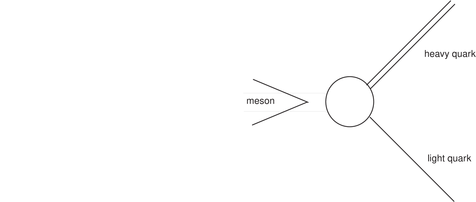
Figure 4: The CQM $Q-{\rm Meson}-q$ vertex.

The vertices for $H$ and $S$ mesons have been derived from bosonization. The vertex involving the $T$ field is instead a phenomenological term, introduced according to the philosophy of effective theories ($\Lambda=1$ GeV in eq. (94)). This value of $\Lambda$ should also be assumed as the ultaviolet cutoff in the regularization of the model $\Lambda=\Lambda_{\chi}$, see the discussion in 2.3.1.

Following [45] we will adopt as UV cutoff $\Lambda=1.25$ GeV. This is a value quite close to the $\Lambda_{\chi}$ discussed in 2.3.1. On the other hand one finds that the CQM phenomenological predictions are not very sensitive to the variation of the UV cutoff, at least if one varies it within $10-15\%$.

Last three terms in (94) are the kinetic terms for $H$, $S$ and $T$ fields. The first two terms come from bosonization, while the third is inserted by hand as a phenomenological term resembling the first two. Bosonization also predicts that $\frac{1}{2G_{3}}=-\frac{1}{2G_{3}^{\prime}}$ and we can therefore write:

$${\cal L}^{hl} = \bar{Q}_{v}(iv\cdot\partial)Q_{v}-\left[\bar{\chi}\left(\bar{H}+\bar{S}+i\bar{T}^{\mu}\frac{\partial^{\mu}}{\Lambda_{\chi}}Q_{v}\right)+h.c.\right]$$ (95)

$$+ \frac{1}{2G_{3}}{\rm Tr}[(\bar{H}+\bar{S})(H-S)]+\frac{1}{2G_{4}}{\rm Tr}[\bar{T}^{\mu}T_{\mu}].$$

The dynamical information $\frac{1}{2G_{3}}=-\frac{1}{2G_{3}^{\prime}}$ is crucial for the CQM calculation of the coupling constants: there are not sufficient experimental data to determine two different constants $G_{3}$ and $G_{3}^{\prime}$.

The kinetic terms will be rewritten, in the form discussed in [35], in the next section, where we will also discuss the problem of determining the mass difference between the $H$ and $S$ multiplets. Again the dynamical information $\frac{1}{2G_{3}}=-\frac{1}{2G_{3}^{\prime}}$ helps this evaluation. We will call $\Delta_{H}$, $\Delta_{S}$ and $\Delta_{T}$ the mass differences between the masses of $H$, $S$ and $T$ multiplets and the heavy quark there contained. The mass difference between $S$ and $H$ will be simply $\Delta_{S}-\Delta_{H}$ and it will be zero as soon as the light constituent quark mass $m\to 0$ (i.e., in the chiral unbroken phase).

3.1.3 Regularization

As we pointed out in 3.1.2, CQM is the fusion of a Manohar-Georgi like Lagrangian for the light quark sector with a quark-meson Lagrangian for the heavy quark sector. We therefore know that the upper energy scale, i.e., the energy scale over which the effective theory should be substituted by a more fundamental theory, is $\Lambda_{\chi}$. It could seem strange that the heavy quark mass is itself higher than the UV cutoff, but we have to remind that in HQET the on shell momentum of the heavy quark, $m_{Q}v$, is not a dynamical quantity since, due to the velocity superselection rule, $v$ is not dynamical, see 2.2. The dynamical quantity due to the interaction between the heavy quark and the light degrees of freedom is the residual momentum $k^{\mu}$, which is necessarily $k\simeq\Lambda_{\rm QCD}<\Lambda_{\chi}$.

CQM does not include the gluon fields, as it is obvious considering that it results from a path integral bosonization of a NJL model, and does not incorporate confinement of quarks. This may appear as a strong limitation of the model but, according to a common opinion, it is physically much more important to work with non confining models possessing chiral symmetry and its spontaneous breakdown than with confining models where chiral symmetry and its breakdown are not properly incorporated. In the former case one is describing a world which is essentially the same as the real one for what concernes the hadronic spectra; the only difference would be that of the theoretical admissibility of asymptotic quark states. The latter case presents an hadronic spectrum completely messed up with respect to the observed one. We show here how one can face the problem that CQM is not a confining model: introducing an infrared cutoff $\mu$.

The kinematical condition for an heavy meson having mass $M$ to decay into its free constituent quarks is:

$$M>m_{Q}+m.$$ (96)

Since the meson momentum is $P=m_{Q}v+k$, where $P=Mv$, eq. (96) is equivalent to the condition $v\cdot k>m$. In the frame where the heavy meson is at rest, the latter condition means $k_{0}>m$, i.e., ${\rm inf}(k)=m$. Therefore one should consider residual momenta $k$ larger than $m$ to be sure that the unphysical threshold condition (96) holds, as it should in a not-confining model. For lower $k$ values one is in the energy region where confinement must be necessarily taken into account.

On the other hand, the value of the constituent light mass is determined by a gap equation (see also (86)) [45]:

$$\langle\Sigma\rangle=m=\tilde{m}+8mI_{1}(m^{2}),$$ (97)

where the chiral ray $\Sigma$ has been defined in (28), while the $I_{1}$ integral is given in the Appendix together with other integrals met in CQM applications. $I_{1}$ is calculated with an UV and an IR cutoff introduced according to the Shwinger’s regularization method, as we will discuss in a while. As the infrared cutoff varies, the $m$ value varies accordingly and, following what we have observed before, we can choice as an infrared cutoff $\mu\simeq m$ (the running momenta in the CQM loops we will deal with, are of the size of the heavy quark residual momenta). In the second paper in reference [45], it is shown the $m$ vs. $\mu$ plot obtained from (97) for a fixed $\Lambda$. This plot has the typical shape of a second order phase transition order parameter with a critical $\mu$ at $\mu_{\rm c}\simeq 550$ MeV. For $\mu>\mu_{\rm c}$, $m$ is zero, i.e., the chiral symmetry is unbroken. For $\mu=m=300$ MeV, one is in the broken (physical) phase at the edge of a plateau.

Therefore the boundary energy values of the effective theory are chosen to be $\mu=300$ MeV, $\Lambda\simeq\Lambda_{\chi}\simeq 1.25$ GeV, and the light constituent mass is dynamically generated by a NJL gap equation: $m=300$ MeV (which represents the degenerate $u$ and $d$ masses. We will not consider $s$ quarks).

The last step is the choice of the prescription to implement the cutoffs in the calculations. For a non renormalizable model, this step is part of the definition of the model itself. The proper time Shwinger regularization has shown to be the most adequate for our purposes.

After a continuation of the light propagator in the Euclidean domain, the following prescription is used:

$$\int d^{4}\ell_{E}\frac{1}{\ell^{2}_{E}+m^{2}}\to\int d^{4}\ell_{E}\int_{1/\Lambda^{2}}^{1/\mu^{2}}dse^{-s(\ell_{E}^{2}+m^{2})}.$$ (98)

All the CQM calculations are performed applying this receipt. If one tries to insert the cutoffs as the bounds of the Euclidean integral measure, besides the problem that Euclidean translation invariance is then lost, one also has to face the problem that the choice of the infrared cutoff is not only conditioned by $m$ (see the discussion made above), but also by $\Delta_{H}$, that is the free parameter of our model. The regularization receipt (98) acts in the sense of modifying the Euclidean light propagator through a factor depending on the difference of two exponential functions of $(\ell^{2}_{E}+m^{2})$. This could affect the Ward-Takahashi relation for, e.g., the vertex of the axial current $A$ with the light quarks, causing the emergence of a mass term for the pion, even if one considers the chiral limit $\partial A=0$ from the beginning. Anyway, due to the structure of the regularization receipt, this should be a very soft effect.

3.2 Renormalization constants and masses

The simplest CQM loop diagram that one can obtain contracting two vertices $Q-{\rm Meson}-q$, see fig. 4, is the meson self energy diagram shown in fig. 5.

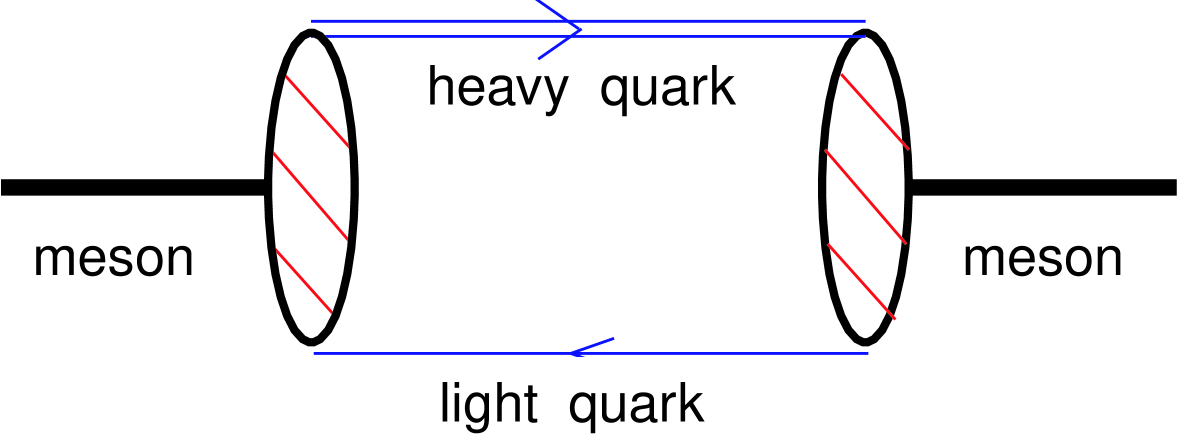
Figure 5: CQM meson self energy diagram.

For in and out $H$ fields, we can write down the following loop integral:

$$iN_{c}\int^{\rm reg}\frac{d^{4}\ell}{(2\pi)^{4}}\frac{{\rm Tr}[H\gamma\cdot(\ell-k+m)\bar{H}]}{[(\ell-k)^{2}-m^{2}+i\epsilon][v\cdot\ell+i\epsilon]}={\rm Tr}[\bar{H}\Pi_{H}(v\cdot k)H].$$ (99)

The rules applied are the standard ones for loop integrals. The expressions of the usual Dirac propagator and of the heavy quark propagator, defined in 2.2, have been inserted in the integral together with the vertex prescriptions derived from the heavy-light Lagrangian ${\cal L}^{hl}$. The regularization procedure is that of the Shwinger’s proper time, see 3.1.3.

First of all let us observe that we can perform the expansion:

$$\Pi(v\cdot k)\simeq\Pi(\Delta)+\Pi^{\prime}(\Delta)(v\cdot k-\Delta),$$ (100)

since we know that $k$ smoothly fluctuates around $(M-m_{Q})v$, i.e.:

$$k^{\mu}=\Delta v^{\mu}-q^{\mu},$$ (101)

where $q$ parameterizes this small fluctuation, see eq. (5), and $\Delta$ is defined as $\Delta=M-m_{Q}$ modulo $1/m_{Q}$ corrections. This expansion of $\Pi$ can now be inserted in the self energy expression for the $H$ field (for $S$ and $T$ fields the procedure is exactly the same) and subtracting from ${\cal L}^{hl}$ the counter-terms ${\rm Tr}[\bar{H}\Pi(v\cdot k)H]$, $-{\rm Tr}[\bar{S}\Pi(v\cdot k)S]$ and $-{\rm Tr}[\bar{T}^{\mu}\Pi(v\cdot k)T_{\mu}]$, one obtains a modified kinetic part of ${\cal L}^{hl}$ that can be written as follows [38]:

$${\cal L}^{hl}_{\rm ren} = -{\rm Tr}[\bar{H}_{\rm ren}(iv\cdot\partial-\Delta_{H})H_{\rm ren}]+{\rm Tr}[\bar{S}_{\rm ren}(iv\cdot\partial-\Delta_{S})S_{\rm ren}]$$ (102)

$$+ {\rm Tr}[\bar{T}_{\rm ren}^{\mu}(iv\cdot\partial-\Delta_{T})T_{\rm ren\mu}],$$

provided that:

$$\frac{1}{2G_{3}} = \Pi_{H}(\Delta_{H})=\Pi_{S}(\Delta_{S})$$ (103)

$$\frac{1}{2G_{4}} = \Pi_{T}(\Delta_{T})$$ (104)

$$H_{\rm ren} = \frac{H}{\sqrt{Z_{H}}}$$ (105)

$$S_{\rm ren} = \frac{S}{\sqrt{Z_{S}}}$$ (106)

$$T_{\rm ren} = \frac{T}{\sqrt{Z_{T}}},$$ (107)

where the renormalization constants $Z$ are defined as follows:

$$Z_{j}^{-1}=\left(\frac{d}{dx}\Pi(x)\right)_{x\to\Delta_{j}},$$ (108)

with $j=H,S,T$. As showed, the kinetic part of ${\cal L}^{hl}$, that originally was written as:

$$\frac{1}{2G_{3}}{\rm Tr}[\bar{H}H]-\frac{1}{2G_{3}}{\rm Tr}[\bar{S}S]+\frac{1}{2G_{4}}{\rm Tr}[\bar{T}^{\mu}T_{\mu}],$$ (109)

it is substituted by the form given in (102), see [35] (see also (71)). If compared with (71) (the expression (102) is extended to include the meson fields $S$ and $T$), (102) does not contain the fields ${\cal V}$, since in the CQM model the pions are not coupling directly to the meson fields and includes mass terms such as $\Delta_{H,S,T}$. In the chiral Lagrangian approach for heavy meson states, see section 2.3.3, the fundamental fields of the Lagrangian are the meson fields. CQM is a somehow more fundamental approach since it includes, together with meson fields, also the quark fields. When one adds in (71) the kinetic terms related to the $S$ and $T$ fields following a chiral Lagrangian approach, see [36], one must also subtract two mass shifting terms: $\delta m_{S}{\rm Tr}[\bar{S}S]$ and $\delta m_{T}{\rm Tr}[\bar{T}^{\mu}T_{\mu}]$, where $\delta m_{S}=m_{S}-m_{H}=\Delta_{S}-\Delta_{H}$ and $\delta m_{T}=m_{T}-m_{H}=\Delta_{T}-\Delta_{H}$ are defined in the $m_{Q}\to\infty$ limit. In the CQM model, that contains explicitly the heavy and light quark fields, $\delta m_{S}$ and $\delta m_{T}$ are substituted by $\Delta_{S}$ and $\Delta_{T}$, i.e., the mass differences between the heavy meson masses $M_{S,T}$ and the mass of the heavy quark involved $m_{Q}$; $\Delta_{H}$ comes in the $H$ kinetic term.

$\Delta_{H}$ is the free CQM parameter. We cannot deduce it from the model, but we can fix it by reasonable numerical values. On the other hand, $\Delta_{S}$ and $\Delta_{T}$ can be computed once $\Delta_{H}$ is fixed. In the case of $\Delta_{S}$, one only needs to solve (103). In the case of $\Delta_{T}$, we will use some experimental information and a $1/m_{Q}$ correction to the meson mass formula (we will discuss this point later on).

The CQM expressions for $\Pi_{H}(\Delta_{H})$, $\Pi_{S}(\Delta_{S})$ and $\Pi_{T}(\Delta_{T})$ are here given. They allow to calculate the renormalization constants $Z_{H,S,T}$:

$$\Pi_{H}(\Delta_{H}) = I_{1}+(\Delta_{H}+m)I_{3}(\Delta_{H})$$ (110)

$$\Pi_{S}(\Delta_{S}) = I_{1}+(\Delta_{S}-m)I_{3}(\Delta_{S})$$ (111)

$$\Pi_{T}(\Delta_{T}) = {1\over{\Lambda_{\chi}^{2}}}\left[-{I^{\prime}_{1}\over 4}+\frac{m+\Delta_{T}}{3}[I_{0}(\Delta_{T})+\Delta_{T}I_{1}+(\Delta_{T}^{2}-m^{2})I_{3}(\Delta_{T})]\right]$$ (112)

$$Z_{H}^{-1} = (\Delta_{H}+m){\frac{\partial I_{3}(\Delta_{H})}{\partial\Delta_{H}}}+I_{3}(\Delta_{H})$$ (113)

$$Z_{S}^{-1} = (\Delta_{S}-m){\frac{\partial I_{3}(\Delta_{S})}{\partial\Delta_{S}}}+I_{3}(\Delta_{S}),$$ (114)

and finally:

$$Z_{T}^{-1} = \frac{1}{3\Lambda^{2}_{\chi}}\Big{[}(\Delta_{T}^{2}-m^{2})\left[(m+\Delta_{T}){\frac{\partial I_{3}(\Delta_{T})}{\partial\Delta_{T}}}+I_{3}(\Delta_{T})\right]$$ (115)

$$+ (m+\Delta_{T})\left[{\frac{\partial I_{0}(\Delta_{T})}{\partial\Delta_{T}}}+I_{1}+2\Delta_{T}I_{3}(\Delta_{T})\right]+I_{0}+\Delta_{T}I_{1}\Big{]},$$

where $\Lambda_{\chi}=1$ GeV. The $I$ integrals are given in the Appendix.

At this point let us fix $\Delta_{H}$ and compute numerically $\Delta_{S,T}$, the couplings $G_{3}$, $G_{4}$ and the renormalization constants $Z_{H,S,T}$.

We will consider everywhere in this work $H_{\rm ren}$, $S_{\rm ren}$ and $T_{\rm ren}$, but often, when notation is evident, we will drop the ‘ren’.

The $\Delta_{H}$ values will be taken in the range $\Delta_{H}=0.3,0.4,0.5$ GeV. $\Delta_{S}$ and $G_{3}$ follow directly from eq. (103). From eqs. (111) and (112) it is evident that $\Delta_{S}-\Delta_{H}=0$ if $m\to 0$. Finally, $\Delta_{T}$ is obtained as follows.

Take $M_{H}$ and $M_{T}$ to be the spin averaged masses related to the $H$ and $T$ multiplets respectively (a weighted average of the experimental masses of the particles in each doublet is taken. The weights are given by the number of polarization states that each particle can assume according to its spin). We can write the following two $O(\frac{1}{m_{Q}})$ equations:

$$M_{H} = m_{Q}+\Delta_{H}+\frac{\Delta_{H}^{\prime}}{m_{Q}}$$ (116)

$$M_{T} = m_{Q}+\Delta_{T}+\frac{\Delta_{T}^{\prime}}{m_{Q}}.$$ (117)

This couple of equations can be written both if $m_{Q}=m_{c}$ or $m_{Q}=m_{b}$.

In the case of $m_{Q}=m_{c}$ we must use experimental information about the $D_{2}^{*}$ and $D_{1}^{*}$ states. As for $D_{2}^{*}$, we have $m_{D^{*}_{2}(2460)^{0}}=2458.9\pm 2.0$ MeV, $\Gamma_{D^{*}_{2}(2460)^{0}}=23\pm 5$ MeV and $m_{D^{*}_{2}(2460)^{\pm}}=2459\pm 4$ MeV, $\Gamma_{D^{*}_{2}(2460)^{\pm}}=25^{+8}_{-7}$ MeV. These particles are identified with the $2^{+}$ states of the $T$ multiplet $\frac{3}{2}^{+}$. As for $D^{*}_{1}(2420)$, experimentally it is found $m_{D^{*}_{1}(2420)^{0}}=2422.2\pm 1.8$ MeV, $\Gamma_{D^{*}_{1}(2420)^{0}}=18.9^{+4.6}_{-3.5}$ MeV; this particle can be identified with the $1^{+}$ state of the $T$ multiplet. We are ignoring a possible small mixing between the $1^{+}$ states belonging respectively to the $S$ and $T$ multiplets [35]. $D_{2}^{*}$ and $D_{1}^{*}$ states are quite broad states since their strong decays proceed in $d$ wave, as pointed out in 2.3.3.

From this analysis we obtain that:

$$\Delta_{T}-\Delta_{H}+\frac{(\Delta^{\prime}_{T}-\Delta^{\prime}_{H})}{m_{c}}\simeq 470{\rm MeV}.$$ (118)

If on the other hand we consider the $m_{Q}=m_{b}$ case, experimental data on positive parity resonances show a bunch of states, not easily resolvable, having a mass $M_{B^{**}}=5698\pm 12$ MeV and a width $\Gamma=128\pm 18$ MeV [49]. If we identify this mass with the $T$ multiplet narrow states mass, we obtain:

$$\Delta_{T}-\Delta_{H}+\frac{(\Delta^{\prime}_{T}-\Delta^{\prime}_{H})}{m_{b}}\simeq 380{\rm MeV}.$$ (119)

Reasonable values of the heavy constituent masses are $m_{b}=m_{B}-300$ MeV and $m_{c}=m_{D}-300$ MeV, where 300 MeV is the constituent mass discussed in 3.1.3, while $m_{B}$ and $m_{D}$ are the experimental masses of the $B$ and $D$ mesons respectively. Solving simultaneously (118) and (119), one gets:

$$\Delta_{T}-\Delta_{H}\simeq 335\;{\rm{MeV}}.$$ (120)

The results for $\Delta_{S}$ and $\Delta_{T}$ as functions of $\Delta_{H}$, are shown in Table 1;

$\Delta_{H}$	$\Delta_{S}$	$\Delta_{T}$
$0.3$	$0.545$	$0.635$
$0.4$	$0.590$	$0.735$
$0.5$	$0.641$	$0.835$

Table 1: $\Delta$ values in (in GeV)

in Table 2 we list the CQM $G_{j}$ and $Z_{j}$ values.

$\Delta_{H}$	$1/G_{3}$	$Z_{H}$	$Z_{S}$	$Z_{T}$	$1/G_{4}$
$0.3$	$0.16$	$4.17$	$1.84$	$2.95$	$0.15$
$0.4$	$0.22$	$2.36$	$1.14$	$1.07$	$0.26$
$0.5$	$0.345$	$1.142$	$0.63$	$0.27$	$0.66$

Table 2: Renormalization constants and couplings. $\Delta_{H}$ in GeV; $G_{3}$, $G_{4}$ in GeV^-2, $Z_{j}$ in GeV^-1.

Through $\Delta_{S}$, CQM predicts the following $m_{S}$ mass value (in literature these are the $D_{0},D_{1}^{*\prime}$ states):

$$m_{S}=2165\pm 50{\rm MeV},$$ (121)

where the central value is given in correspondence of $\Delta_{H}=0.4$ GeV, while the upper and lower values are related to the remaining two $\Delta_{H}$ values. This determination does not account for $1/m_{c}$ corrections (see eqs. (116) and (117)). These states are very difficult to be observed experimentally since of their large width: from [50] one expects $\Gamma(D_{0}\to D^{+}\pi^{-})\simeq 180$ MeV and $\Gamma(D_{1}^{*\prime}\to D^{*+}\pi^{-})\simeq 165$ MeV. Theoretical predictions of $m_{S}$ available in literature are anyway larger, a typical value is $m_{S}=2350$ MeV. Very recent CLEO data [51] indicate, as the mass of the $S$ multiplet, $m_{S}=2461$ MeV. This discrepancy of about $300$ MeV between CQM and experimental data can be attributable to the absence of $O(1/m_{c})$ corrections in CQM calculations. Anytime we will need to use $m_{S}$ in applications, we will use both the CQM predicted value, for consistency, and the experimental one.

3.3 ${\cal L}^{ll}$ extension to include $\rho$ and $a_{1}$ resonances.

The effective Lagrangian (93) for the CQM light sector can be extended to include $\rho$ and $a_{1}$ resonances. The operative hypothesis needed is that of Vector-Meson-Dominance (VMD) (and of Axial-Meson-Dominance for $a_{1}$). We will briefly sketch the VMD hypothesis: then the insertion of $\rho$ in ${\cal L}^{ll}$ (analogously for $a_{1}$) will turn out to be a simple step.

Let us consider the electromagnetic form factor for $\pi^{+}$:

$$\langle\pi^{+}(p^{\prime})|J_{\mu}|\pi^{+}(p)\rangle=(p+p^{\prime})_{\mu}F_{\pi}(t).$$ (122)

where $t=(p^{\prime}-p)^{2}$. The best way to determine this form factor is to consider the process $\gamma p\to n\pi^{+}$ where $\gamma$ is a virtual photon coming from the scattering of an electron [52]. Now one does the hypothesis that $F_{\pi}(t)$ is an analytic function in the variable $t$ with a branching cut on the real positive axis. This hypothesis allows to write the following dispersion relation for $F_{\pi}$:

$$F_{\pi}(t)=\frac{1}{\pi}\int_{4m_{\pi}^{2}}^{\infty}dt^{\prime}\frac{{\cal I}m(F_{\pi}(t^{\prime}))}{t^{\prime}-t}.$$ (123)

The lower integration bound is the threshold above which the form factor is different from zero. Observe that for $t\to\infty$ one has $F_{\pi}(t)\to 0$, since the probability of producing only two pions, when an enormous number of higher energy states are accessible, is extremely low.

Let us suppose that $F_{\pi}(t)$ is dominated by the $\rho^{0}$ resonance (VMD-hypothesis) in such a way that one can write, for the absorbitive part [53]:

$${\cal I}m(F_{\pi}(t^{\prime}))\propto\delta(t^{\prime}-m_{\rho}^{2}).$$ (124)

Then we have that:

$$F_{\pi}(t)=\frac{m_{\rho}^{2}}{m_{\rho}^{2}-t}.$$ (125)

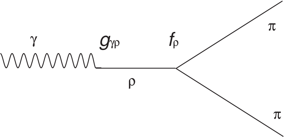
Figure 6: $\gamma-\rho$ coupling diagram.

On the other hand, if we consider the diagram in fig. 6 [54], where the $\gamma-\rho$ coupling is shown, we can write:

$$eF_{\pi}(t)=\frac{g_{\gamma\rho}f_{\rho}}{m_{\rho}^{2}-t},$$ (126)

where the $f_{\rho}$ coupling with pions is an universal coupling, i.e., is the same with two nucleons, two $\rho$’s, etc. $f_{\rho}$’s universality is a consequence of electric charge conservation and of the complete $\rho$ dominance.

From eqs. (125,126) we conclude that the $\gamma-\rho$ coupling constant is given by:

$$g_{\gamma\rho}=e\frac{m_{\rho}^{2}}{f_{\rho}}.$$ (127)

In a paper by N.M. Kroll, T.D. Lee and B. Zumino [55], it is shown that, at lower order in $e$, it makes sense to consider the interaction of an interpolating $\rho$ field, $\frac{m_{\rho}^{2}}{f_{\rho}}\rho^{\mu}$, with the photon:

$$e\frac{m_{\rho}^{2}}{f_{\rho}}\rho^{\mu}A_{\mu},$$ (128)

even if this term shows to be manifestly not gauge-invariant (one can prove that introducing an $e^{2}$ term in the interaction Lagrangian, this problem is solved). Equation (128) can be considered as the coupling of the gauge field with the current:

$$J_{\mu}=\frac{m_{\rho}^{2}}{f_{\rho}}\rho_{\mu}.$$ (129)

This identity between the $\rho$ interpolating field and the $J_{\mu}$ current makes sense only if $\rho^{\mu}$ is coupled to a conserved external current, as one can easily show writing the Lagrangian for the $\rho^{\mu}$ field as:

$${\cal L}^{\rho}=-\frac{1}{4}(F_{\mu\nu})^{2}-\frac{1}{2}m_{\rho}^{2}\rho^{\mu}\rho_{\mu}+j\cdot\rho,$$ (130)

where an interaction $j\cdot\rho$ with an external current $j$ (the $\rho$ source) is included. If one takes the divergence of the equation of motion derivable from (130), and if one considers that $\partial\cdot J=0$, then one has $\partial\cdot j=0$. The equation of motion is:

$$(\partial^{2}+m^{2})\rho^{\mu}=j^{\mu}.$$ (131)

Eq. (131) produces the following relation between matrix elements:

$$\langle B|J^{\mu}|A\rangle=\frac{m_{\rho}^{2}}{f_{\rho}}\frac{\langle B|j^{\mu}|A\rangle}{m^{2}_{\rho}-t}.$$ (132)

Therefore, at the level of matrix elements, we can see that the $\rho$ and the photon sources coincide, modulo a factor $\frac{1}{f_{\rho}}$. A problem arises if one observes that $f_{\rho}$ is not directly measurable at $t=0$, due to the finite $\rho$ mass: in $\rho\to\pi\pi$ one measures $f_{\rho}$ for $t=m^{2}_{\rho}\neq 0$. This means that one has to formulate the problematic hypothesis that $f_{\rho}$ is essentially constant in the $(0,m_{\rho}^{2})$ interval (in this respect VMD is similar to PCAC). This problem is even stronger for $a_{1}$, that has a mass larger than the $\rho$ one by a factor of $3/2$.

Let us go back to CQM. We can couple the $\rho$ interpolating field to the vector fermion light quark current:

$$\frac{m_{\rho}^{2}}{f_{\rho}}\rho_{\mu}\bar{\chi}\gamma^{\mu}\chi.$$ (133)

The same thing can be made for $a_{1}$, writing an analog interaction for the $a_{1}$ interpolating field. These interaction terms give Feynman rules for CQM vertices between light quark current -$\rho$, -$a_{1}$:

$$\rho\leavevmode\nobreak\ {\rm vertex} = i\frac{m_{\rho}^{2}}{f_{\rho}}\gamma^{\mu}\epsilon_{\mu}^{*}$$ (134)

$$a_{1}\leavevmode\nobreak\ {\rm vertex} = i\frac{m_{a_{1}}^{2}}{f_{a_{1}}}\gamma^{\mu}\gamma_{5}\epsilon_{\mu}^{\prime*},$$ (135)

where $\epsilon$ and $\epsilon^{\prime}$ are the polarizations of $\rho$ and $a_{1}$ respectively.

The expression for the CQM effective Lagrangian ${\cal L}^{ll}$, must incorporate these results. Let us write ${\cal L}^{ll}$ using a notation mediated by the Hidden-Symmetry approach, which incorporates VMD [39]:

$${\cal L}^{ll} = {f_{\pi}^{2}\over 8}\partial_{\mu}\Sigma^{\dagger}\partial^{\mu}\Sigma+\frac{1}{2g_{V}^{2}}{\rm Tr}[{\cal F(\rho)}_{\mu\nu}{\cal F(\rho)}^{\mu\nu}]+\frac{1}{2g_{A}^{2}}{\rm Tr}[{\cal F}(a)_{\mu\nu}{\cal F}(a)^{\mu\nu}]$$ (136)

$$+ {\bar{\chi}}(iD^{\mu}\gamma_{\mu}-m)\chi$$

$$+ {\bar{\chi}}({\cal A}^{\mu}\gamma_{\mu}\gamma_{5}-ih_{\rho}\rho^{\mu}\gamma_{\mu}-ih_{a}a^{\mu}\gamma_{\mu}\gamma_{5})\chi,$$

where:

$${\cal F}(x)_{\mu\nu}=\partial_{\mu}x_{\nu}-\partial_{\nu}x_{\mu}+[x_{\mu},x_{\nu}],$$ (137)

describes the strength tensor for the $\rho$ and $a_{1}$ fields. Moreover:

$$\rho_{\mu}=i\frac{g_{V}}{\sqrt{2}}{\hat{\rho}}_{\mu}\leavevmode\nobreak\ \leavevmode\nobreak\ \leavevmode\nobreak\ \leavevmode\nobreak\ \leavevmode\nobreak\ \leavevmode\nobreak\ \leavevmode\nobreak\ \leavevmode\nobreak\ \leavevmode\nobreak\ \leavevmode\nobreak\ \leavevmode\nobreak\ \leavevmode\nobreak\ g_{V}=\frac{m_{\rho}}{f_{\pi}}\simeq 5.8$$ (138)

and, in an analogous way, we also write ($m_{a}\simeq 1.26$ GeV):

$$a_{\mu}=i\frac{g_{A}}{\sqrt{2}}{\hat{a}}_{\mu}\leavevmode\nobreak\ \leavevmode\nobreak\ \leavevmode\nobreak\ \leavevmode\nobreak\ \leavevmode\nobreak\ \leavevmode\nobreak\ \leavevmode\nobreak\ \leavevmode\nobreak\ \leavevmode\nobreak\ \leavevmode\nobreak\ \leavevmode\nobreak\ \leavevmode\nobreak\ g_{A}=\frac{m_{a}}{f_{\pi}}\simeq 9.5,$$ (139)

where $\hat{\rho}$ and $\hat{a}$ are Hermitian $3\times 3$ matrices related to positive and negative parity light mesons. If we consider:

$$h_{\rho} = \frac{\sqrt{2}m^{2}_{\rho}}{g_{V}f_{\rho}}$$ (140)

$$h_{a} = \frac{\sqrt{2}m^{2}_{a}}{g_{A}f_{a}},$$ (141)

then we are implementing VMD and AMD hypotheses and we are recovering (134,135) vertices. Numerically one finds:

$$h_{\rho}\simeq h_{a}\simeq 0.95.$$ (142)

For us $f_{\rho}=0.152\leavevmode\nobreak\ {\rm GeV}^{2}$, as emerges from $\rho^{0}$ and $\omega$ decays in $e^{+}e^{-}$, and $f_{a}=0.25\pm 0.02\leavevmode\nobreak\ {\rm GeV}^{2}$, as it comes out from $\tau\to\nu_{\tau}\pi\pi\pi$ decay [57]. This result agrees with a determination made for $f_{a}$ by QCD sum rules [58]. Lattice QCD predicts $f_{a}=0.30\pm 0.03\leavevmode\nobreak\ {\rm GeV}^{2}$, [59]. Since $1/f_{a}$ multiplies all amplitudes containing the $a_{1}$ meson, the uncertainty on $f_{a}$ will induce an uncertainty on normalizations for all the amplitudes involving the light axial meson.

4 Strong Couplings

4.1 Processes with one $\pi$ in the final state

This is the first of two sections where the CQM model will be used to compute the coupling constants for the strong decays $H\to H\pi$, $S\to H\pi$, $S\to S\pi$, $T\to H\pi$, $T\to S\pi$ and $H\to H(\rho,a_{1})$, $H\to S(\rho,a_{1})$. A technique allowing to go beyond the soft pion limit hypothesis is also introduced. As showed previously, CQM incorporates a direct coupling of the pion to the light quark current. For strong processes with one pion in the final state, there is only one CQM diagram describing the decay of an heavy meson to another heavy meson and a pion. This diagram is represented in fig. 7. Different processes have different in and out heavy meson states and the soft pion limit hypothesis must be discussed case by case. The soft pion limit allows to simplify calculations, but it is a rough approximation if, e.g., transitions $S\to H\pi$ or $T\to H\pi$ are considered. In the exact chiral limit we can write, for the pion momentum, $q^{\mu}=(q_{\pi},0,0,q_{\pi})$ . In the heavy meson rest frame, $v=(1,0,0,0)$, we have $v\cdot q=q_{\pi}$. Moreover $v\cdot q=v\cdot(p-p^{\prime})=\Delta_{S}-\Delta_{H}\neq 0$, where $p$ and $p^{\prime}$ denote the momenta of the in and out mesons respectively and we have used the relation $v\cdot k=\Delta$, $k$ being the residual momentum, (see 2.2), and $\Delta$ the mass difference between the heavy meson and the heavy quark there contained. Therefore, the soft pion limit is not very reliable for transitions such as $S\to H\pi$, where $\Delta_{S}-\Delta_{H}\simeq 140-190$ MeV. We should observe that, if we adopt the soft pion limit hypothesis, the CQM diagram of fig. 7 shows a very soft NG boson emitted from an internal line of a diagram, while we should have expeced an Adler zero of the emitting amplitude in this case. Anyway the CQM regularization scheme forces $\ell^{2}$ in the loop to be quite close to $m^{2}$ and this saves the soft pion approximation (see discussion in [33], pp. 175,176).

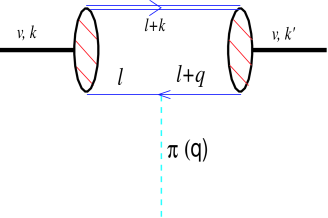
Figure 7: CQM diagram for transitions meson $\to$ meson $+$ pion.

In [38] the calculation of CQM amplitudes for the transitions $H\to H\pi$ and $S\to H\pi$ has been performed using in both cases the soft pion limit, which works as a good approximation only in the first case. In [40], a technique allowing to avoid the soft pion limit has been introduced for the $T\to H\pi$ process. The same technique gives the possibility of improving also the $S\to H\pi$ calculation. Evidently, the soft pion limit is a good approximation for the $S\to S\pi$ process [42]. Recent CLEO data [51] indicate that $m_{S}\simeq m_{T}\simeq 2460$ MeV so that the soft pion limit may be used also for the $T\to S\pi$ process [42]. In the next two subsections we will show how to compute the mentioned processes in the soft and not-soft pion hypothesis.

4.1.1 $H\to H\pi$, the soft pion limit

Let’s consider the first term in the Lagrangian (72):

$${\cal L}=ig{\rm Tr}[\bar{H}H\gamma\cdot{\cal A}\gamma_{5}],$$ (143)

where the meson field $H$ has been defined in (64). The transition $1^{-}\to 0^{-}\pi$ is allowed. We can therefore consider $\langle D\pi|i{\cal L}|D^{*}\rangle$ and, using (143), we obtain:

$$\langle D\pi|i{\cal L}|D^{*}\rangle=g\left(-\frac{iq^{\mu}}{f_{\pi}}\right){\rm Tr}[\tilde{P}\gamma_{5}\frac{1+\gamma\cdot v}{2}\gamma^{\sigma}\tilde{P}^{*}_{\sigma}\gamma_{\mu}\gamma_{5}],$$ (144)

where ${\cal A}$ has been expanded up to the first order in $\pi$ and the zeroth order in the expansion has been neglected. Observing that $\tilde{P}=\langle H|P|{\rm VAC}\rangle$ and $\tilde{P}^{*}_{\sigma}=\langle{\rm VAC}|P^{*}_{\sigma}|H\rangle$ can be made explicit using (66,67), the interaction term (144) reduces to:

$$-ig\frac{2m_{H}}{f_{\pi}}(\epsilon\cdot q),$$ (145)

where $\epsilon$ represents the polarization of the $1^{-}$ state. As already observed, this interaction effective Lagrangian describes the coupling of the pion to the meson states, the fundamental fields at low energy, see fig. 8.

Figure 8: In the low energy language of chiral Lagrangians, the pion is directly coupled to the meson fields.

In the CQM model, where the fundamental fields are the heavy and light constituent quarks, the same coupling is modeled as a coupling of the pion to the light quark current. Figure 7 shows a one loop CQM diagram containing two vertices meson-$Q$-$\chi$, see fig. 4, described by ${\cal L}^{hl}$ introduced in (95) and one vertex pion-$\chi\chi$. This diagram can be computed as a standard loop diagram in the following way:

$$(-1)i^{3}i^{3}Z_{H}m_{H}\frac{N_{c}}{16\pi^{4}}\int d^{4}\ell\frac{{\rm Tr}[(\gamma\cdot\ell+m)(-\frac{q^{\mu}}{f_{\pi}}\gamma_{\mu}\gamma_{5})(\gamma\cdot\ell+m)\gamma_{5}\frac{1+\gamma\cdot v}{2}\gamma^{\sigma}\epsilon_{\sigma}]}{(\ell^{2}-m^{2})^{2}(v\cdot\ell+\Delta_{H})}.$$ (146)

Here is a legenda for the factors appearing in the preceding expression:

• $(-1)$ from the fermion loop
  

• $i^{3}$ from the three quark propagators
  

• $i^{3}$ from the Feynman rules for the $\chi\chi\pi$ vertex, described in ${\cal L}^{ll}$, and for the two $\chi HQ$ vertices, described in ${\cal L}^{hl}$; both carry a factor of $(-i)$
  

• $Z_{H}$ is due to the fact that the two meson fields coming in the loop integral must be the renormalized fields, $\sqrt{Z_{H}}$ being the renormalization constant
  

• $m_{H}$ comes from the normalization conditions (66,67)
  

• $N_{c}$ is the number of colours running in the loop ($N_{c}=3$)
  

• $(-\frac{q^{\mu}}{f_{\pi}}\gamma_{\mu}\gamma_{5})$ is the one pion expansion of the $\gamma\cdot{\cal A}\gamma_{5}$ term contained in ${\cal L}^{ll}$.
  

At this point one should calculate the trace in (146) and the following integrals:

$$Z = \frac{iN_{c}}{16\pi^{4}}\int d^{4}\ell\frac{1}{(\ell^{2}-m^{2})^{2}(v\cdot\ell+\Delta_{H})}$$ (147)

$$Z_{\mu} = \frac{iN_{c}}{16\pi^{4}}\int d^{4}\ell\frac{\ell_{\mu}}{(\ell^{2}-m^{2})^{2}(v\cdot\ell+\Delta_{H})}$$ (148)

$$Z_{\mu\nu} = \frac{iN_{c}}{16\pi^{4}}\int d^{4}\ell\frac{\ell_{\mu}\ell_{\nu}}{(\ell^{2}-m^{2})^{2}(v\cdot\ell+\Delta_{H})}.$$ (149)

The technique for calculating $Z$ with the proper time regularization procedure will be explained in detail in the next section, where the general case in which the two light propagators carry different momenta ($\ell$ and $\ell+q$ respectively) is analyzed. The soft pion approximation is achieved performing the $q_{\pi}\to 0$ limit. The expression for $Z$ is then equivalent to the expression for $I_{4}(\Delta_{H})$ given in the Appendix. The Lorentz structures must be treated as in the following example:

$$Z_{\mu\nu}=\frac{iN_{c}}{16\pi^{4}}\int d^{4}\ell\frac{\ell_{\mu}\ell_{\nu}}{(\ell^{2}-m^{2})^{2}(v\cdot\ell+\Delta_{H})}=Qv_{\mu}v_{\nu}+Rg_{\mu\nu}.$$ (150)

In order to obtain $Q$ and $R$, the contraction with $v^{\mu}v^{\nu}$ and $g^{\mu\nu}$ in needed. In such a way one obtains integrals of the type described in the Appendix.

A comparison between (145) and (146) shows that, in order to obtain $g$, one has to extract from (146) the coefficient of $\epsilon\cdot q$. The CQM expression for $g$ is then the following:

$$g=Z_{H}\left[\frac{1}{3}I_{3}(\Delta_{H})-2\left(m+\frac{1}{3}\Delta_{H}\right)(I_{2}+\Delta_{H}I_{4}(\Delta_{H}))-\frac{4}{3}m^{2}I_{4}(\Delta_{H})\right],$$ (151)

where all the $I$ integrals are listed in the Appendix. Numerically:

$$g=0.456\pm 0.040,$$ (152)

where the central value corresponds to $\Delta_{H}=0.4$ GeV and the lower (higher) values, correspond to $\Delta_{H}=0.3$ GeV ($\Delta_{H}=0.5$ GeV). These values agree with what is found using the QCD sum rules method, $g=0.44\pm 0.16$ [35, 60]. A good aggreement is also found with relativistic quark models giving $g\simeq 0.40$ [61] and $g=0.34$ [62]. CQM disagrees with the determination by Le Yaouanc and Becirevic [63] according to which $g=1$.

The coupling constant $g$ allows the determination of the hadronic width:

$$\Gamma(D^{*+}\to D^{0}\pi^{+})=\frac{g^{2}}{6\pi f_{\pi}^{2}}|{\vec{p}_{\pi}}|^{3}.$$ (153)

Numerical values are described in Table 3.

Decay	$\Delta_{H}=0.4$ GeV	$\Delta_{H}=0.5$ GeV	Exp.
${D^{*}}^{0}\to D^{0}\pi^{0}$	$65.5$	$70.1$	$61.9\pm 2.9$
${D^{*}}^{0}\to D^{0}\gamma$	$34.5$	$29.9$	$38.1\pm 2.9$
${D^{*}}^{+}\to D^{0}\pi^{+}$	$71.6$	$71.7$	$68.3\pm 1.4$
${D^{*}}^{+}\to D^{+}\pi^{0}$	$28.0$	$28.1$	$30.6\pm 2.5$
${D^{*}}^{+}\to D^{+}\gamma$	$0.4$	$0.24$	$1.1^{+2.1}_{-0.7}$

Table 3: Theoretical and experimental B.R.’s for $D^{*}$. The theoretical values are computed for $\Delta_{H}=0.4,0.5$ GeV.

Table 3, following [38], includes also the B.R.’s predicted by CQM for the radiative decays. The CQM calculation of radiative processes proceeds without qualitatively new elements with respect to what explained so far.

The soft pion approximation is also suitable for the $S\to S\pi$ process [42]. The meson interaction Lagrangian is given by the second term in eq. (72):

$${\cal L}=ig^{\prime}{\rm Tr}[\bar{S}S\gamma\cdot{\cal A}\gamma_{5}].$$ (154)

Once calculated the CQM loop diagram, a comparison with the mesonic amplitude $\langle S\pi|i{\cal L}|S\rangle$ gives:

$$g^{\prime}=Z_{S}\left[\frac{1}{3}I_{3}(\Delta_{S})-2\left(-m+\frac{1}{3}\Delta_{S}\right)(I_{2}+\Delta_{S}I_{4}(\Delta_{S}))-\frac{4}{3}m^{2}I_{4}(\Delta_{S})\right],$$ (155)

to which correspond the numerical values:

$$g^{\prime}=-0.13\pm 0.04.$$ (156)

Observe that $g^{\prime}$ can be obtained by $g$ with the simple exchange $m\to-m$, $\Delta_{H}\to\Delta_{S}$ and $Z_{H}\to Z_{S}$. Indeed the loop integral for the process $1^{+}\to 0^{+}\pi$ can be obtained by the loop integral for $H\to H\pi$, shifting the $\gamma_{5}$ matrix contained in (146) on the right side of $\gamma_{\sigma}$. In so doing, one writes the expression that would have written for the $S\to S\pi$ process but having $-\gamma\cdot v$, instead of $\gamma\cdot v$, in the projector. Expanding the trace in (146) in it’s four terms different from zero, one realizes that this substitution in the projector is equivalent to an $m\to-m$ exchange.

According to the CLEO data, $m_{S}\simeq m_{T}$, therefore the soft pion limit is a good approximation also for $T\to S\pi$. The CQM approach gives [42]:

$$f=2\sqrt{Z_{T}Z_{S}}[mV-T],$$ (157)

where $V$ and $T$ are linear combinations of the $I_{i}$ integrals discussed in the Appendix, while $f$ is defined in (73). Numerically we find:

$$f=0.91^{+0.56}_{-0.27}.$$ (158)

4.1.2 $T\to H\pi$, $q_{\pi}\neq 0$

Let’s go back to the integral $Z$ given in eq. (147) and evaluate it in the general case of pions bringing a momentum $q_{\pi}\neq 0$:

$$Z=\frac{iN_{c}}{16\pi^{4}}\int\frac{d^{4}\ell}{(\ell^{2}-m^{2})((\ell+q)^{2}-m^{2})(v\cdot\ell+\Delta+i\epsilon)},$$ (159)

where the Feynman contour prescription is made explicit in the expression for the heavy quark propagator. Since the pion is the NG boson of the broken chiral symmetry, we put:

$$q^{\mu}=(q_{\pi},0,0,q_{\pi}).$$ (160)

Let’s write (159) in the following way:

$$Z=H_{1}+H_{2} = \int^{\rm reg}\frac{d^{4}\ell}{(\ell^{2}-m^{2})((\ell+q)^{2}-m^{2})(v\cdot\ell+\Delta-i\epsilon)}$$ (161)

$$- 2\pi i\int^{\rm reg}d^{4}\ell\frac{\delta(v\cdot\ell+\Delta)}{(\ell^{2}-m^{2})((\ell+q)^{2}-m^{2})},$$

where the proper time regularization is concerned and the Plemelij identity has been invoked [64]:

$$\frac{1}{x-(x_{0}\pm i\epsilon)}={\rm P.V.}\frac{1}{x-x_{0}}\pm i\pi\delta(x-x_{0}),$$ (162)

in such a way that poles with negative real part lie in the upper complex $\ell_{0}$ plane.

As a first step we compute $H_{1}$:

$$H_{1} = \frac{d}{dm^{2}}\int^{\rm reg}d^{4}\ell\int_{0}^{1}\frac{dx}{((\ell+qx)^{2}-m^{2})(v\cdot\ell+\Delta)}$$ (163)

$$= -i\frac{d}{dm^{2}}\int d^{4}\ell_{E}\int_{0}^{1}\frac{dx}{((\ell+qx)^{2}_{E}+m^{2})(i\ell_{4}+\Delta)}$$

$$= -\frac{d}{dm^{2}}\int d^{4}\ell_{E}\int_{0}^{1}\frac{dx}{(\ell^{2}_{E}+m^{2})(\ell_{4}-i\Delta(x))}.$$

In the first equation the Feynman integral trick has been used while, in the second, the Euclidean rotation is performed. At this stage $q_{4}=-iq_{\pi}$ and we can shift $\ell_{4}\to\ell^{\prime}_{4}+iq_{\pi}x$ as shown in the last equation in (163). Here $\Delta(x)=\Delta-q_{\pi}x$. Now we must exponentiate the light quark propagator and cutoff the integrals according to the Shwinger’s proper time prescription described in 3.1.3. We recall also the numerical factor $\frac{iN_{c}}{16\pi^{4}}$ and write ($N_{c}=3$):

$$H_{1} = -\frac{iN_{c}}{16\pi^{4}}\frac{d}{dm^{2}}\int_{1/\Lambda^{2}}^{1/\mu^{2}}dse^{-sm^{2}}\int d^{3}{\bf{\bf\ell}}e^{-s{\bf\ell}^{2}}\int d\ell_{4}\frac{e^{-s\ell_{4}^{2}}}{\ell_{4}-i\Delta(x)}$$ (164)

$$= -\frac{3}{16\pi^{3/2}}\int_{1/\Lambda^{2}}^{1/\mu^{2}}ds\frac{e^{-sm^{2}}}{s^{1/2}}\int_{0}^{1}dxe^{s\Delta^{2}(x)}(1-{\rm erf}(\sqrt{s}\Delta(x))).$$

In the second equation we have used the following formula:

$$\frac{1}{i\pi}\int dt\frac{e^{-t^{2}}}{t-iz}=e^{z^{2}}(1-{\rm erf}(z)),$$ (165)

where:

$${\rm erf}(z)=\frac{2}{\sqrt{\pi}}\int_{0}^{z}dte^{-t^{2}}.$$ (166)

In a similar way let’s work out $H_{2}$:

$$H_{2} = -2\pi i\frac{d}{dm^{2}}\int^{\rm reg}d^{4}\ell\int_{0}^{1}dx\frac{\delta(\ell_{0}+\Delta)}{((\ell+qx)^{2}-m^{2})}$$ (167)

$$= -2\pi\frac{d}{dm^{2}}\int d^{4}\ell_{E}\int_{0}^{1}dx\frac{\delta(i\ell_{4}+\Delta)}{((\ell+qx)^{2}_{E}+m^{2})}$$

$$= -2\pi\frac{d}{dm^{2}}\int d^{4}\ell_{E}\int_{0}^{1}dx\frac{\delta(i\ell_{4}+\Delta(x))}{(\ell^{2}_{E}+m^{2})}$$

$$= 2\pi i\frac{d}{dm^{2}}\int d^{3}\ell\int_{0}^{1}dx\int_{1/\Lambda^{2}}^{1/\mu^{2}}dse^{-s(m^{2}+{\bf{\bf\ell}}^{2}-\Delta^{2}(x))}$$

$$= 2\frac{3}{16\pi^{3/2}}\int_{1/\Lambda^{2}}^{1/\mu^{2}}ds\frac{e^{-sm^{2}}}{s^{1/2}}\int_{0}^{1}dxe^{s\Delta^{2}(x)},$$

where the same steps as for $H_{1}$ have been followed. In the last equation $\frac{iN_{c}}{16\pi^{4}}$ is taken into account. Summing the expressions obtained for $H_{1}$ and $H_{2}$:

$$Z=\frac{3}{16\pi^{3/2}}\int_{1/\Lambda^{2}}^{1/\mu^{2}}ds\frac{e^{-sm^{2}}}{s^{1/2}}\int_{0}^{1}dxe^{s\Delta^{2}(x)}(1+{\rm erf}(\sqrt{s}\Delta(x))).$$ (168)

The soft pion limit amounts to consider $q_{\pi}\to 0$, $\Delta(x)\to\Delta$ and therefore $Z\to I_{4}(\Delta)$, where $I_{4}(\Delta)$, given in the Appendix, comes from the integration of (147). The CQM calculation of the process $T\to H\pi$ [40], requires not only the calculation of $Z$, but also of $Z_{\mu}$, $Z_{\mu\nu}$ and $Z_{\mu\nu\lambda}$ since the CQM loop integral for $T\to H\pi$ is:

$$-\frac{i}{2f_{\pi}}\sqrt{Z_{H}Z_{T}m_{H}m_{T}}q^{\mu}\eta^{\sigma\nu}\frac{iN_{c}}{16\pi^{4}}\int^{\mathrm{reg}}d^{4}\ell\frac{{\rm Tr}[(\gamma\cdot\ell+m)\gamma_{\mu}\gamma_{5}(\gamma\cdot(\ell+q)+m)\gamma_{5}(1+\gamma\cdot v)\gamma_{\nu}k_{\sigma}]}{(\ell^{2}-m^{2})[(\ell+q)^{2}-m^{2}](v\cdot\ell+\Delta)}.$$ (169)

Let’s consider, for example, $Z_{\mu\nu}=Cv_{\mu}v_{\nu}+Dq_{\mu}q_{\nu}+E(v_{\mu}q_{\nu}+q_{\mu}v_{\nu})+Og_{\mu\nu}$. If we contract both members of this equation with the tensors $v_{\mu}v_{\nu}$, $q_{\mu}q_{\nu}$,..we obtain a linear system of four simultaneous equations to be solved with respect to $C,D,E,O$, knowing the (integral) expressions $v^{\mu}v^{\nu}Z_{\mu\nu}$, $q^{\mu}q^{\nu}Z_{\mu\nu}$, $v^{\mu}q^{\nu}Z_{\mu\nu}$ and $g^{\mu\nu}Z_{\mu\nu}$. The matrix ${\bf A}$, acting on the vector $(C,D,E,O)$, contains powers of $q_{\pi}$ multiplied by numerical factors. The hadronic matrix element that one wants to compute, informs about the powers of $q_{\pi}$ that should be eliminated in ${\bf A}$.

Let’ recall now the eq. (170):

$${\cal L}=\frac{h_{1}}{\Lambda_{\chi}}{\rm Tr}[\bar{H}T^{\mu}(iD_{\mu}\gamma\cdot{\cal A})\gamma_{5}]+\frac{h_{2}}{\Lambda_{\chi}}{\rm Tr}[\bar{H}T^{\mu}(i\gamma\cdot D{\cal A}_{\mu})\gamma_{5}]+{\rm h.c.}$$ (170)

Using the same strategy followed in the calculation of $g$ in 4.1, we find that $h^{\prime}=h_{1}+h_{2}$ is given by [40]:

$$h^{\prime} = \sqrt{Z_{T}Z_{H}}\Big{\{}\frac{m^{2}}{q_{\pi}}\Big{[}I_{2}+\Delta_{T}Z(\Delta_{T})+\frac{1}{2q_{\pi}}(I_{3}(\Delta_{H})-I_{3}(\Delta_{T}))\Big{]}$$ (171)

$$+ P(R_{i}(\Delta_{T}),S_{i}(\Delta_{T}),q_{\pi})\Big{\}}.$$

The polynomial $P(R_{i},S_{i},q_{\pi})$, given in the Appendix, is a sum of $q_{\pi}$ powers multiplied by some linear combinations of the integrals $I_{i}$ and $Z$ that we called $R_{i}$ and $S_{i}$. If we write down the hadronic matrix elements for the processes $T\to H\pi$ (the following three), $S\to H\pi$ and $H\to H\pi$ (the last two), we understand that, e.g., in the CQM calculation of $h^{\prime}$ one should take account only of two powers of $q_{\pi}$, therefore we neglect terms $O(q_{\pi}^{3})$ (e.g., in ${\bf A}$).

$$\langle D^{+}(p^{\prime})\pi^{-}(q)|D_{2}^{*0}(p,\eta)\rangle = ig_{1}\eta^{\mu\nu}q_{\mu}q_{\nu}$$ (172)

$$\langle D^{*+}(p^{\prime},\epsilon)\pi^{-}(q)|D_{2}^{*0}(p,\eta)\rangle = ig_{2}\eta^{\mu\nu}q_{\mu}\epsilon_{\lambda\sigma\nu\tau}\epsilon^{*\lambda}\frac{p^{\sigma}}{m_{T}}q^{\tau}$$ (173)

$$\langle D^{*+}(p^{\prime},\epsilon)\pi^{-}(q)|D_{1}^{*0}(p,\eta)\rangle = ig_{3}\eta_{\nu}\epsilon^{*}_{\sigma}[3q^{\nu}q^{\sigma}+g^{\nu\sigma}\left(q^{2}-\frac{(p\cdot q)^{2}}{m_{T}}\right)]$$ (174)

$$\langle D^{0}(p^{\prime})\pi^{+}(q)|D_{0}^{+}(p)\rangle = ig_{4}\frac{m_{S}^{2}-m_{H}^{2}}{m_{S}}$$ (175)

$$\langle D^{0}(p^{\prime})\pi^{+}(q)|D^{*+}(p,\epsilon)\rangle = ig_{5}q^{\mu}\epsilon_{\mu}.$$ (176)

The processes involving the $c$ quark are the most interesting since the charmed states, even the positive parity ones, are object of wide experimental investigation. The coupling constants $g_{1},..,g_{5}$ are connected to the coupling constants appearing at the level of meson Lagrangians by the following relations:

$$g_{1} = g_{2}=2\sqrt{m_{H}m_{T}}\frac{h^{\prime}}{\Lambda_{\chi}f_{\pi}}$$ (177)

$$g_{3} = \sqrt{\frac{2m_{H}m_{T}}{3}}\frac{h^{\prime}}{\Lambda_{\chi}f_{\pi}}$$ (178)

$$g_{4} = \sqrt{m_{H}m_{S}}\frac{f^{\prime}}{f_{\pi}}$$ (179)

$$g_{5} = \frac{2m_{H}}{f_{\pi}}g,$$ (180)

where $f^{\prime}$ has been introduced in (73).

Using recent data on the masses [49] and the CQM value for $h^{\prime}=0.65$, one obtaines the following widths:

$$\Gamma(D_{2}^{*0}\to D^{+}\pi^{-}) = 4.59\times 10^{7}\frac{h^{\prime 2}}{\Lambda_{\chi}^{2}}\leavevmode\nobreak\ {\rm MeV}=19.4\leavevmode\nobreak\ {\rm MeV}$$ (181)

$$\Gamma(D_{2}^{*0}\to D^{*+}\pi^{-}) = 1.33\times 10^{7}\frac{h^{\prime 2}}{\Lambda_{\chi}^{2}}\leavevmode\nobreak\ {\rm MeV}=5.6\leavevmode\nobreak\ {\rm MeV}$$ (182)

$$\Gamma(D_{1}^{*0}\to D^{*+}\pi^{-}) = 1.47\times 10^{7}\frac{h^{\prime 2}}{\Lambda_{\chi}^{2}}\leavevmode\nobreak\ {\rm MeV}=6.2\leavevmode\nobreak\ {\rm MeV}.$$ (183)

Due to the neutral pion decay channel, these widths should be multiplied by a factor of $1.5$.

According to the chiral Lagrangian for heavy mesons, the total width of the state $D_{2}^{*0}$ is dominated by decays with only one pion in the final state. Therefore we can use the experimental value for this width, $23\pm 5$ MeV, to obtain $h^{\prime}_{\rm exp}=0.51$, in good agreement with $h^{\prime}=0.65$ predicted by CQM.

Equation (183) gives the total width for $D_{1}^{*0}$ decaying to one pion, i.e., $\Gamma=9.3$ MeV. This is only one half of the measured total width $18.9^{+4.6}_{-3.5}$ MeV. This effect could be attributed to a mixing of $T(1^{+})$ with $S(1^{+})$ or to strong $O(1/m_{c})$ corrections [65].

4.1.3 $S\to H\pi$, $q_{\pi}\neq 0$

Applying the technique developed in 4.1.2, we can compute the strong coupling $f^{\prime}$ describing $S\to H\pi$. One finds:

$$f^{\prime}=\sqrt{Z_{S}Z_{H}}\left[R_{1}(\Delta_{S})-R_{2}(\Delta_{S})-\frac{R_{4}(\Delta_{S})}{q_{\pi}}+m^{2}Z(\Delta_{S})\right].$$ (184)

In this computation only terms up to order $q_{\pi}^{1}$ have been considered. Numerically we find:

$$f^{\prime}=-0.76\pm 0.13,$$ (185)

where the error is induced by the variation of $\Delta_{H}$ in the range $0.3,0.4,0.5$ GeV. In this computation the CQM value $m_{S}=2.165\pm 0.05$ GeV has been used (the error in this last determination doesn’t affect much the $f^{\prime}$ numerical value). Anyway, recent CLEO data [51] give $m_{S}\simeq 2.461$ GeV for the broad charmed state $S(1^{+})$. This discrepancy between the experimental value and the CQM determination, is most likely due to $O(1/m_{c})$ corrections. Since $m_{S}$ determines the $q_{\pi}$ value, the experimental value gives a different numerical result for $f^{\prime}$:

$$f^{\prime}=-0.56\pm 0.11,$$ (186)

consistent with a QCD sum rules determination [50]:

$$f^{\prime}=-0.52\pm 0.17.$$ (187)

If one computes the process $S\to H\pi$ applying the soft pion limit hypothesis, the following numerical determination for $f^{\prime}$ is obtained [38]:

$$f^{\prime}=-0.85\pm 0.02.$$ (188)

Neglecting mixing effects $S(1^{+})-T(1^{+})$ we can evaluate the width of $D_{1}^{\prime}$ using the CLEO results for $m_{S}$ and the CQM value for $f^{\prime}$. We get:

$$\Gamma(D_{1}^{\prime}\to D^{*}\pi)=240\;{\rm MeV},$$ (189)

which probably accounts for the entire $D_{1}^{\prime}$ width, due to the limited phase space. This result can be compared with the CLEO total width for the $1^{+}$ state, $290^{+101}_{-79}\pm 26\pm 36$ MeV.

4.2 Processes with $\rho$ and $a_{1}$ in the final state

In this section we will discuss the strong coupling constants $HH\rho$, $HS\rho$, $HHa_{1}$ and $HSa_{1}$. These will turn out to be essential when the semileptonic decays $B\to(\rho,a_{1})\ell\nu$ [39] are examined. According to the notations introduced in [35], these couplings are parametrized in the following way:

$${\cal L}_{HH\rho} = i\lambda{\mathrm{Tr}}(\overline{H}H\sigma^{\mu\nu}{\cal F(\rho)}_{\mu\nu})-i\beta{\mathrm{Tr}}(\overline{H}H\gamma^{\mu}\rho_{\mu})$$ (190)

$${\cal L}_{HS\rho} = -i\zeta{\mathrm{Tr}}(\overline{S}H\gamma^{\mu}\rho_{\mu})+i\mu{\mathrm{Tr}}(\overline{S}H\sigma^{\mu\nu}{\cal F(\rho)}_{\mu\nu})$$ (191)

$${\cal L}_{HHa_{1}} = -i\zeta_{A}{\mathrm{Tr}}(\overline{H}H\gamma^{\mu}a_{\mu})+i\mu_{A}{\mathrm{Tr}}(\overline{H}H\sigma^{\mu\nu}{\cal F}(a)_{\mu\nu})$$ (192)

$${\cal L}_{HSa_{1}} = i\lambda_{A}{\mathrm{Tr}}(\overline{S}H\sigma^{\mu\nu}{\cal F}(a)_{\mu\nu})-i\beta_{A}{\mathrm{Tr}}(\overline{S}H\gamma^{\mu}a_{\mu}).$$ (193)

The CQM approach for the determination of these constants amounts to a loop calculation of diagrams like the one in fig. 7, where the pion is substituted by a $\rho$ or $a_{1}$ according to the Feynman rules obtained in 3.3, followed by a comparison with the hadronic matrix elements determined by the interaction Lagrangians above listed.

Even if the strategy is the same as before, we have some new technical difficulties in dealing with $\rho$ and $a_{1}$, partly because of the polarizations of these states, partly because of the fact that $\rho$ and $a_{1}$ are not massless.

The first mentioned problem has influence on the expressions for the hadronic matrix elements. Consider, for example, the transition $H(1^{-})\to S(0^{+})\rho$. This process has contributions in $s$ and $d$ wave. The $d$ wave contribution comes only from the Lagrangian term containing the factor $\mu$ in (191) while, the $s$ wave contributions, come also from the Lagrangian term containing the $\zeta$ factor. With obvious notation, the matrix element is written in the following way:

$$\langle\rho^{+}(\epsilon,q)S(p^{\prime})|H(\eta,p)\rangle=-i\epsilon^{*}_{\mu}\eta_{\lambda}(Sg^{\mu\lambda}+Dv^{\mu}q^{\lambda}).$$ (194)

Applying the notations introduced in 3.3, we can compute explicitly the traces in (191) obtaining:

$$S = \frac{g_{V}}{\sqrt{2}}\sqrt{m_{H}m_{S}}(2\zeta-4\mu(v\cdot q))$$ (195)

$$D = \frac{g_{V}}{\sqrt{2}}\sqrt{m_{H}m_{S}}(4\mu).$$ (196)

Therefore to obtain $S$ and $D$, a CQM calculation of $\zeta$ and $\mu$ is required. Similar considerations apply for matrix elements containing the $T$ state.

Since $\rho$ and $a_{1}$ are not massless particles, the loop integral $Z$, given in (197), must be examined in the case of a general $q$ ($q^{2}\neq 0$) momentum. Once that $Z$ is computed, the problem of determining $Z_{\mu}$, $Z_{\mu\nu}$,..is consequential.

As we know, $Z$ is given by:

$$Z=\frac{iN_{c}}{16\pi^{4}}\int\frac{d^{4}\ell}{(\ell^{2}-m^{2})((\ell+q)^{2}-m^{2})(v\cdot\ell+\Delta+i\epsilon)}.$$ (197)

Let’s consider the following identity:

$$\frac{1}{(\ell^{2}-m^{2})}\frac{1}{((\ell+q)^{2}-m^{2})}=\frac{1}{q^{2}+2\ell\cdot q}\left[\frac{1}{(\ell^{2}-m^{2})}-\frac{1}{((\ell+q)^{2}-m^{2})}\right],$$ (198)

where $q$ is, e.g., the $\rho$ momentum. Then we can write:

$$q^{\mu}=m_{\rho}v^{\prime\mu}.$$ (199)

Therefore, considering transitions $(1)\to(2)\rho$ with (1) and (2) generic in and out meson states in the CQM diagram and calling $x$ the mass value of $\rho$ or $a_{1}$, the following expression for $Z$ easily follows:

$$Z=\frac{iN_{c}}{32x\pi^{4}}\int\frac{d^{4}\ell}{(\ell^{2}-m^{2})}\left[\frac{1}{(v\cdot\ell+\Delta_{1})(v^{\prime}\cdot\ell+\frac{x}{2})}-\frac{1}{(v\cdot\ell+\Delta_{2})(v^{\prime}\cdot\ell-\frac{x}{2})}\right],$$ (200)

where:

$$v\cdot v^{\prime}=\frac{v\cdot q}{x}=\frac{\Delta_{1}-\Delta_{2}}{x}.$$ (201)

Applying the notations given in the Appendix, $Z$ can be also be written as:

$$Z=\frac{I_{5}(\Delta_{1},x/2,\omega)-I_{5}(\Delta_{2},-x/2,\omega)}{2x},$$ (202)

where $\omega=v\cdot v^{\prime}$ and this equation is well defined for all $\omega$ values. At this point, we must care of integrals with several Lorentz indices:

$$Z^{\mu} = \Omega_{1}v^{\mu}+\Omega_{2}v^{\prime\mu}$$ (203)

$$Z^{\mu\nu} = \Omega_{3}g^{\mu\nu}+\Omega_{4}v^{\mu}v^{\nu}+\Omega_{5}v^{\prime\mu}v^{\prime\nu}+\Omega_{6}[v^{\mu}v^{\prime\nu}+v^{\prime\mu}v^{\nu}],$$ (204)

where the $\Omega_{i}$ are reported in the Appendix. The CQM results for $\lambda$ and $\beta$ are:

$$\lambda = \frac{m^{2}_{\rho}}{\sqrt{2}g_{V}f_{\rho}}Z_{H}(-\Omega_{1}+mZ)$$ (205)

$$\beta = \sqrt{2}\frac{m^{2}_{\rho}}{g_{V}f_{\rho}}Z_{H}[2m\Omega_{1}+m_{\rho}\Omega_{2}+2\Omega_{3}-\Omega_{4}+\Omega_{5}-m^{2}Z].$$ (206)

Here the functions $Z$, $\Omega_{j}$ are computed with $\Delta_{1}=\Delta_{2}=\Delta_{H}$, $x=m_{\rho}$, $\omega=m_{\rho}/(2m_{B})$ where one takes the first $1/m_{Q}$ correction to $\omega=0$. Moreover:

$$\mu = \frac{m^{2}_{\rho}}{\sqrt{2}g_{V}f_{\rho}}\sqrt{Z_{H}Z_{S}}\left(-\Omega_{1}-2\frac{\Omega_{6}}{m_{\rho}}+mZ\right)$$ (207)

$$\zeta = \frac{\sqrt{2}m^{2}_{\rho}}{g_{V}f_{\rho}}\sqrt{Z_{H}Z_{S}}\left(m_{\rho}\Omega_{2}+2\Omega_{3}+\Omega_{4}+\Omega_{5}-m^{2}Z\right),$$ (208)

where $\Delta_{1}=\Delta_{H}$, $\Delta_{2}=\Delta_{S}$, $x=m_{\rho}$ and $\omega=(\Delta_{1}-\Delta_{2})/{m_{\rho}}$.

The axial couplings of $a_{1}$ to $H$ and $S$ are here listed:

$$\lambda_{A} = \frac{m^{2}_{a}}{\sqrt{2}g_{A}f_{a}}\sqrt{Z_{H}Z_{S}}\left(-\Omega_{1}+2\Omega_{2}\frac{m}{m_{a}}+mZ\right)$$ (209)

$$\beta_{A} = \sqrt{2}\frac{m^{2}_{a}}{g_{A}f_{a}}\sqrt{Z_{H}Z_{S}}(m_{a}\Omega_{2}+2\Omega_{3}-\Omega_{4}+\Omega_{5}+m^{2}Z),$$ (210)

where now $\Delta_{1}=\Delta_{H}$, $\Delta_{2}=\Delta_{S}$, $x=m_{a}$ and $\omega=(\Delta_{1}-\Delta_{2})/{m_{a}}$. Moreover:

$$\mu_{A} = \frac{m^{2}_{a}}{\sqrt{2}g_{A}f_{a}}Z_{H}\left(m\left(Z+2\frac{\Omega_{2}}{m_{a}}\right)-\Omega_{1}-2\frac{\Omega_{6}}{m_{a}}\right)$$ (211)

$$\zeta_{A} = \frac{\sqrt{2}m^{2}_{a}}{g_{A}f_{a}}Z_{H}(-2m\Omega_{1}+m_{a}\Omega_{2}+2\Omega_{3}+\Omega_{4}+\Omega_{5}+m^{2}Z),$$ (212)

where $\Delta_{1}=\Delta_{H}$, $x=m_{a}$, $\omega=m_{a}/(2m_{B})$. Numerically the results are:

$$\begin{array}[]{cclcccl}\lambda&=&0.60\leavevmode\nobreak\ {\rm{GeV}}^{-1}&&\lambda_{A}&=&0.85\times(0.25\leavevmode\nobreak\ {\rm GeV}^{2}/f_{a})\leavevmode\nobreak\ {\rm{GeV}}^{-1}\\ \beta&=&-0.86&&\beta_{A}&=&-0.81\times(0.25\leavevmode\nobreak\ {\rm GeV}^{2}/f_{a})\\ \mu&=&0.16\leavevmode\nobreak\ {\rm{GeV}}^{-1}&&\mu_{A}&=&0.23\times(0.25\leavevmode\nobreak\ {\rm GeV}^{2}/f_{a})\leavevmode\nobreak\ {\rm{GeV}}^{-1}\\ \zeta&=&0.01&&\zeta_{A}&=&0.15\times(0.25\leavevmode\nobreak\ {\rm GeV}^{2}/f_{a}).\end{array}$$

As already mentioned, $f_{a}$ is the principal source of theoretical error on these results. Another source of uncertainty is the variation of $\Delta_{H}$ in the range $\Delta_{H}=0.3-0.5$ GeV (above we have used only the $\Delta_{H}=0.4$ GeV value). The latter produces a significative uncertainty only in the $\zeta,\beta_{A},\zeta_{A}$ determination since $\zeta=0.01\pm 0.19$, $\beta_{A}=-0.81^{+0.45}_{-0.24}$ and $\zeta_{A}=0.15^{+0.16}_{-0.14}$ while, in the other cases, only a few percent variation is observed. A theoretical uncertainty of $\pm 15\%$ can be added to the constants $\lambda$, $\mu$, $\lambda_{A}$, $\mu_{A}$. This follows, for example, from the calculation of $\lambda$ performed in [38] for the processes $B^{*}\to B\gamma$ and $D^{*}\to D\gamma$. Other evaluations of the of $\lambda$ can be found in [66] and [67].

5 Semileptonic decays

5.1 Semileptonic decays: leptonic constants

CQM, as all constituent quark models, can only give model-dependent predictions that do not have the features of theoretical solidity achievable by the SVZ sum rules approach [4] or by lattice QCD. Anyway, effective constituent quark models are sometimes easy to use tools allowing to evaluate the hadronic matrix elements.

One of the main goals of the next future experimental physics is the high precision measurement of CKM matrix elements $V_{cb}$ and $V_{ub}$; $B$ physics experiments, such as Belle [68] and BaBar [69], are already running in this direction. The semileptonic decays play a central role for the determination of CKM elements, therefore, a wide set of theoretical predictions for these processes, is a very actual need.

In the next sections we will consider how CQM can help this need. The greatest part of the results we will obtain have already been determined through other approaches.

The first target will be the determination of $s$ and $p$ wave semileptonic $B$ decays to charmed mesons. The Isgur-Wise form factors governing the hadronic matrix elements relative to these processes will be calculated through CQM loop diagrams where an external weak current interacts with the heavy quark internal line, inducing a boost on the velocity of the heavy quark and possibly a change in its flavor.

Next we will consider the semileptonic decays $B\to\rho\ell\nu$ and $B\to a_{1}\ell\nu$. An experimental determination by CLEO [70, 49] gives a branching ratio for the former amounting to:

$${\cal B}(B^{0}\to\rho^{-}\ell^{+}\nu)=(2.5\pm 0.4^{+0.5}_{-0.7}\pm 0.5)\;\times\;10^{-4}.$$ (213)

This process offers an important test for CQM.

Experimental information are instead missing in the $B\to a_{1}\ell\nu$ channel. CQM has given the first prediction for the branching ratio of this process. A QCD sum rule prediction for the same process has been recently carried out in a paper by Aliev and Savci [71]. Discrepancies with this work will be discussed later on.

A role of prominent importance in the determination of $V_{ub}$ is covered by the semileptonic channel $B\to\pi\ell\nu$ and a precise measure of this process is one of the major goals of $B$-factories. CQM predicts a new contribution to the form factors governing $B\to\pi\ell\nu$. This new contributions are due to CQM diagrams in which the $\pi$ is directly attached to the $B$ loop. They influence the form factors inducing corrections between $10\%$ and $30\%$, according to the moment carried away by the weak current.

Let’s start with the evaluation of the leptonic constants $\hat{F}$ and $\hat{F}^{+}$ through diagrams of the kind of that in fig. 9. These constants will be useful to calculate the so called polar contribution to $B\to\rho$, $B\to a_{1}$. Their definition is:

$$\langle{\rm VAC}|{\bar{q}}\gamma^{\mu}\gamma_{5}Q|H(0^{-},v)\rangle = i\sqrt{m_{H}}v^{\mu}{\hat{F}}$$ (214)

$$\langle{\rm VAC}|{\bar{q}}\gamma^{\mu}Q|S(0^{+},v)\rangle = i\sqrt{m_{S}}v^{\mu}{\hat{F}}^{+}.$$ (215)

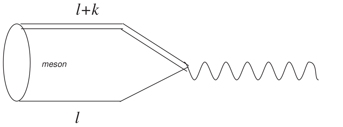
Figure 9: CQM diagram for the lepton decay constants.

Computing the loop diagram given in fig. 9, with the CQM rules one easily finds:

$${\hat{F}} = \frac{\sqrt{Z_{H}}}{G_{3}}$$ (216)

$${\hat{F}}^{+} = \frac{\sqrt{Z_{S}}}{G_{3}},$$ (217)

where the renormalization constants $Z$ and the coupling constant $G_{3}$ have been discussed in 3.2. The calculation proceeds following the usual CQM strategy: from the loop integral one extracts the $v^{\mu}$ contribution and a comparison with the matrix elements (214) and (215) gives $\hat{F}$ and $\hat{F}^{+}$. The numerical values are given in Table 4.

$\Delta_{H}$	${\hat{F}}$	${\hat{F}}^{+}$
$0.3$	$0.33$	$0.22$
$0.4$	$0.34$	$0.24$
$0.5$	$0.37$	$0.27$

Table 4: ${\hat{F}}$ and ${\hat{F}}^{+}$ for three $\Delta_{H}$ values. $\Delta_{H}$ is expressed in GeV; leptonic constants are in GeV^3/2.

Neglecting logarithmic corrections, ${\hat{F}}$ and ${\hat{F}}^{+}$ are connected, in the $m_{Q}\to\infty$ limit, to the leptonic decay constants $f_{B}$ and $f^{+}$:

$$\langle 0|{\bar{q}}\gamma^{\mu}\gamma_{5}b|B(p)\rangle = ip^{\mu}f_{B}$$ (218)

$$\langle 0|{\bar{q}}\gamma^{\mu}b|B_{0}(p)\rangle = ip^{\mu}f^{+},$$ (219)

through the relations $f_{B}={\hat{F}}/\sqrt{m_{B}}$ and $f^{+}={\hat{F}}^{+}/\sqrt{m_{B_{0}}}$. For example, if $\Delta_{H}=400$ MeV, one obtains:

$$f_{B} \simeq 150\;{\rm{MeV}}$$ (220)

$$f^{+} \simeq 100\;{\rm{MeV}}.$$ (221)

The QCD sum rules analysis [72] gives ${\hat{F}}=0.30\pm 0.05$ GeV^3/2, neglecting radiative corrections and even higher values, $0.4-0.5$ GeV^3/2, including $\alpha_{s}$ corrections. Another QCD sum rules analysis [73] suggests ${\hat{F}}^{+}=0.46\pm 0.06$ GeV^3/2, which is somehow higher with respect to the CQM values. Lattice QCD [74] gives $f_{B}=170\pm 35$ MeV.

5.2 $b\to c$ transitions

We are interested in studying some weak heavy meson decays, i.e., decays with flavor changing of the heavy quark due to the presence of the charged weak current $W$. Let’s focus on the $b\to c\ell\bar{\nu}$ transitions. Such processes are described by the following four fermion operator:

$${\cal O}=\frac{G_{F}V_{cb}}{\sqrt{2}}\bar{c}\gamma^{\mu}(1-\gamma_{5})b\bar{\nu}\gamma_{\mu}(1-\gamma_{5})\ell.$$ (222)

At the quark level one can calculate the matrix element:

$${\rm Amp}_{q}=\langle c\ell\bar{\nu}|{\cal O}|b\rangle=\frac{G_{F}V_{cb}}{\sqrt{2}}\bar{u}_{c}(p_{c})\gamma^{\mu}(1-\gamma_{5})u_{b}(p_{b})\bar{u}_{\nu}(p_{\nu})\gamma_{\mu}(1-\gamma_{5})u_{\ell}(p_{\ell}),$$ (223)

that is relevant only at very small distances and fails when, as is the case in the hadron world, quarks cannot be treated as asymptotic states. The hadronic amplitude ${\rm Amp}_{h}$ is:

$${\rm Amp}_{h}=\langle D^{*}\ell\bar{\nu}|{\cal O}|B\rangle=\frac{G_{F}V_{cb}}{\sqrt{2}}\langle D^{*}|\bar{c}\gamma^{\mu}(1-\gamma_{5})b|B\rangle\langle\ell\bar{\nu}|\bar{\nu}\gamma_{\mu}(1-\gamma_{5})\ell|{\rm VAC}\rangle.$$ (224)

The hadronic matrix term in ${\rm Amp}_{h}$ accounts for non perturbative QCD effects. It is possible to parameterize these effects through form factors depending on $q^{2}$, where $q$ is the momentum carried by the weak current. Strong interaction symmetries, and in particular HQET symmetries (in the limit $m_{Q}\to\infty$), have influence on the properties of these form factors. Many times this influence acts in the sense of simplification, reducing the number of form factors needed to parameterize the matrix element.

5.2.1 The Isgur-Wise function $\xi(\omega)$

Let’s consider an elastic scattering process $B(v)\to B(v^{\prime})$ mediated by the weak current $V_{\mu}$. A model of what happens in the hadron is the following: due to the action of the weak current, the heavy quark is suddenly substituted by another heavy quark having the same flavor but different velocity $v^{\prime}$. Light degrees of freedom must rearrange themselves in order to give rise to a $B$ meson moving with velocity $v^{\prime}$. This rearranging process is mediated by an exchange of soft gluons (having momenta of order $\simeq\Lambda_{\rm QCD}$) with the heavy quark acting as the source of chromoelectric field. The larger is $v^{\prime}-v$, the smaller is the probability to have an elastic transition: we have a suppression of the elastic form factor. In the $m_{b}\to\infty$ limit, the form factor can only depend on $v$ and $v^{\prime}$ in the scalar combination $v\cdot v^{\prime}=\omega$. We can introduce a dimensionless probability function, $\xi(\omega)$, that works as the form factor of the transition. This function is known, in HQET, as the Isgur-Wise function:

$$\langle\bar{B}(v^{\prime})|\bar{h}_{v^{\prime}}\gamma^{\mu}h_{v}|\bar{B}(v)\rangle=m_{B}\xi(\omega)(v+v^{\prime})^{\mu},$$ (225)

where $m_{B}$ is due to a particular choice of the normalization of the external meson states. To convince oneself that there are no terms proportional to $(v-v^{\prime})$, it is sufficient to multiply the matrix element in (225) by $(v-v^{\prime})_{\mu}$ and remind from section 2.2 that $\gamma\cdot vh_{v}=h_{v}$ and $h_{v}\gamma\cdot v=h_{v}$.

The interpretation of $\xi(\omega)$, as the probability for the elastic transition $B(v)\to B(v^{\prime})$, suggests to assign a value of $\xi=1$ when $\omega=1$, i.e., when there is no change of velocity; smaller probability values (form factor suppression) are assigned when $v\neq v^{\prime}$.

We can examine this point in greater detail. The $\xi(\omega)$ function describes the response of light degrees of freedom to the change of velocity of the static source of colour. This change can also be accompanied by a flavor change of the heavy quark. If $v=v^{\prime}$, the current causing the transition is therefore a symmetry current since light degrees of freedom do not resolve the flavor of the heavy quark (this is the flavor symmetry of HQET). This symmetry current comes together with conserved charges, generators of the flavor symmetry, which are connected to the current by the well known relation:

$$Q^{f^{\prime}f}=\int d^{3}xh^{+\prime}_{v}(x)h_{v}(x),$$ (226)

where $f^{\prime}=f$ means that the current hasn’t produced heavy quark flavor change. One can verify explicitly that the weak current responsible for the $\omega=1$ transition is a conserved current:

$$\partial_{\mu}\bar{h}^{\prime}_{v}v^{\mu}h_{v}=0,$$ (227)

where the property $\gamma\cdot vh_{v}=h_{v}$ and the equation of motion derived by (23) have been used.

Meson states must be eigenstates of charge operators in such a way that:

$$Q^{f^{\prime}f}|P(v)\rangle = |P^{\prime}(v)\rangle$$ (228)

$$Q^{ff}|P(v)\rangle = |P(v)\rangle,$$ (229)

where $P$ denotes a pseudoscalar meson (let’s simplify the discussion taking the case of $J=0$ mesons). If we write:

$$\langle P^{\prime}(v^{\prime})|\bar{h}^{\prime}_{v^{\prime}}\gamma^{\mu}h_{v}|P(v)\rangle=m_{P}\xi(\omega)(v+v^{\prime})^{\mu},$$ (230)

and if we consider $v=v^{\prime}$, take the $\mu=0$ component, integrate with respect to ${\bf x}$ and use the (228), we get:

$$\xi(1)=1,$$ (231)

assuming the following meson state normalization:

$$\langle M(p^{\prime})|M(p)\rangle=2m_{M}v^{0}(2\pi)^{3}\delta^{3}({\bf p}-{\bf p}^{\prime}).$$ (232)

The normalization condition $\xi(\omega=1)=1$ is particularly relevant not only because it is connected to the flavor symmetry of HQET, but also because it is not affected by $1/m_{Q}$ corrections. The relevant corrections are $O(1/m_{Q}^{2})$. This is consequence of the Luke theorem [75], generalization of the Ademollo-Gatto theorem [76], according to which, at $\omega=1$, there are no corrections to the hadronic matrix elements responsible for the semileptonic decays $B\to D\ell\bar{\nu}$ and $B\to D^{*}\ell\bar{\nu}$. The leading corrections to the normalization of these matrix elements are, at the zero recoil point, of order $1/m_{c}^{2}$. Since $\Lambda_{\rm QCD}^{2}/m_{c}^{2}\simeq 10\%$, zeroth order predictions in the $1/m_{c}$ expansion are, for $\omega=1$, very accurate. Far from the zero recoil point $\omega=1$, corrections of order $1/m_{c}$ are suppressed by $(\omega-1)$ factors.

The normalization condition $\xi(1)=1$ is therefore a good table test to understand if CQM allows for a correct calculation of the Isgur-Wise function.

Let’s go back to the weak transitions $b\to c$. The decay $b\to c$ is mediated by the left-handed current $J^{\mu}=\bar{c}\gamma^{\mu}(1-\gamma_{5})b$. This operator not only carries momentum, but also rotates the orientation of the the spin $s_{Q}$ of the heavy quark during its decay. For an assigned value of total angular momentum of the light degrees of freedom $s_{\ell}$, the relative orientation of $s_{Q}$ determines if the hadron in its final state is a $D$ or $D^{*}$. The heavy quark spin symmetry induces relations connecting the matrix elements for the decays $B\to D\ell\nu$, $B\to D^{*}\ell\nu$ in such a way that they could be expressed in terms of a unique universal form factor $\xi(\omega)$.

Let’s consider for example the following matrix element:

$$\langle D(p^{\prime})|V^{\mu}|B(p)\rangle=f_{+}(q^{2})(p+p^{\prime})^{\mu}+f_{-}(q^{2})(p-p^{\prime})^{\mu},$$ (233)

where $V^{\mu}$ is the vectorial component of $J^{\mu}$. In HQET one has :

$$\langle D(p^{\prime})|V^{\mu}|B(p)\rangle=\sqrt{m_{B}m_{D}}\xi(\omega)(v+v^{\prime})^{\mu}.$$ (234)

Therefore we can see a relation between (233) and (234):

$$f_{\pm}=C_{cb}\frac{m_{D}\pm m_{B}}{2\sqrt{m_{B}m_{D}}}\xi(\omega),$$ (235)

where $C_{cb}$ is the correction that emerges from the matching with QCD, see 2.2.2. In the following we will consider $C_{cb}=1$ for simplicity. In an analogous way one can consider the matrix elements describing the processes $B\to D^{*}$, where $V^{\mu}$ and $A^{\mu}$ are both relevant. One finds:

$$\langle D(v^{\prime})|{\bar{c}}\gamma_{\mu}(1-\gamma_{5})b|B(v)\rangle = \sqrt{m_{B}m_{D}}\;\xi(\omega)(v_{\mu}+v^{\prime}_{\mu})$$ (236)

$$\langle D^{*}(v^{\prime},\epsilon)|{\bar{c}}\gamma_{\mu}(1-\gamma_{5})b|B(v)\rangle = \sqrt{m_{B}m_{D^{*}}}\;\xi(\omega)[i\epsilon_{\mu\nu\alpha\beta}\epsilon^{*\nu}v^{\prime\alpha}v^{\beta}$$ (237)

$$- (1+\omega)\epsilon^{*}_{\mu}+(\epsilon^{*}\cdot v)v^{\prime}_{\mu}].$$

In order to determine $\xi(\omega)$ with CQM, one needs to calculate the loop diagram in fig. 10.

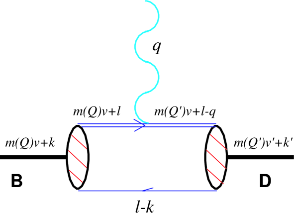
Figure 10: Weak current insertion on the heavy quark propagator line.

We will address the simple case in which $Q=Q^{\prime}=b$. Let’s observe that the momentum $q$ is given by:

$$q=(m_{b}v+k)-(m_{b}v^{\prime}+k^{\prime}),$$ (238)

and the momentum carried by the heavy quark having $v^{\prime}$ velocity is then:

$$m_{b}v+\ell-q=m_{b}v^{\prime}+\ell+k^{\prime}-k,$$ (239)

where we have used the relation (238). Using the CQM approach developed in so far, one can write the loop integral describing the diagram of fig. 10 in the following way:

$$m_{H}Z_{H}(-1)i^{3}i^{2}\frac{N_{c}}{16\pi^{4}}\int d^{4}\ell\frac{{\rm Tr}\left[(\gamma\cdot(\ell-k)+m)(-\gamma_{5})\frac{1+\gamma\cdot v^{\prime}}{2}\gamma^{\mu}\frac{1+\gamma\cdot v}{2}\gamma_{5}\right]}{((\ell-k)^{2}-m^{2})(v^{\prime}\cdot(\ell+k^{\prime}-k))(v\cdot\ell)},$$ (240)

where for simplicity we are considering as in and out states the pseudoscalar mesons of the $H$ multiplet. We can perform the shift $\ell-k\to\ell$ and, observing that $v\cdot k=v^{\prime}\cdot k^{\prime}=\Delta_{H}$, we can rewrite (240) in the following way:

$$m_{H}Z_{H}(-1)i^{3}i^{2}\frac{N_{c}}{16\pi^{4}}\int d^{4}\ell\frac{{\rm Tr}\left[(\gamma\cdot\ell+m)(-\gamma_{5})\frac{1+\gamma\cdot v^{\prime}}{2}\gamma^{\mu}\frac{1+\gamma\cdot v}{2}\gamma_{5}\right]}{(\ell^{2}-m^{2})(v^{\prime}\cdot\ell+\Delta_{H})(v\cdot\ell+\Delta_{H})}.$$ (241)

Once computed the trace, $\xi(\omega)$ is extracted by comparison with the transition amplitude (225).

The CQM expression for $\xi(\omega)$ is:

$$\xi(\omega)=Z_{H}\left[\frac{2}{1+\omega}I_{3}(\Delta_{H})+\left(m+\frac{2\Delta_{H}}{1+\omega}\right)I_{5}(\Delta_{H},\Delta_{H},\omega)\right],$$ (242)

where the $I_{i}$ integrals are listed in the Appendix. Let’s observe that $I_{5}(\Delta,\Delta,1)=\frac{\partial}{\partial\Delta}I_{3}(\Delta)$. Recalling the equation (113), we then have [38]:

$$\xi(1)=1,$$ (243)

as expected.

A very accurate determination of $V_{cb}$ can be obtained measuring the recoil spectrum of $D^{*}$ produced in semileptonic decays of $B$. In particular, measuring the differential decay rate for $\bar{B}\to D^{*}\ell\nu$, one obtains an indirect measure of the product $V_{cb}\xi(\omega)$. If we expand $\xi(\omega)$ around $\omega=1$ and if we suppose $\xi(1)=1$ (taking into account $1/m_{Q}^{2}$ corrections and bound state effects gives a value of $\xi(1)\simeq 0.91$ [17]), then near $\omega=1$:

$$(1-\rho^{2}_{IW}(\omega-1))V_{cb},$$ (244)

where $\rho^{2}_{IW}$, defined by:

$$\rho^{2}_{IW}=-\frac{d\xi}{d\omega}(1),$$ (245)

works as a fit parameter allowing to extrapolate back to the $V_{cb}$ value that one could measure at zero recoil.

The CQM numerical values for $\rho^{2}_{IW}$ are given in Table 5. What emerges is that CQM results are in a quite good agreement with those obtained with QCD sum rules: $\rho^{2}_{IW}=0.54-1.0$ [77]. After an overall examination of the results obtained for the Isgur-Wise function in a series of quark models [78, 79, 80, 81], authors in [82] find $\rho^{2}_{IW}=0.97-1.28$. Lattice QCD indicates lower results, around $\rho^{2}_{IW}=0.64$ [83].

In fig. 11 it is shown a plot of the $\xi(\omega)$ given in (242).

Figure 11: Isgur-Wise form factor vs. $\omega$ for different $\Delta_{H}$ values.

5.2.2 $\tau_{1/2}(\omega)$ and $\tau_{3/2}(\omega)$ form factors

In this section we will consider the semileptonic decays of an $H$ meson to $S$ and $T$ mesons. These decays are written as:

$$B\to D^{**}\ell\nu,$$ (246)

where $D^{**}$ can be either an $S$ state, i.e., a charmed meson $0^{+}$ or $1^{+}$ with $s_{\ell}=1/2$, or a $T$ state, i.e., a charmed meson $2^{+}$ or $1^{+}$ with $s_{\ell}=3/2$. There are two form factors describing respectively these decays: they are known as $\tau_{1/2}$ and $\tau_{3/2}$ [84]. The relevant matrix elements are:

$$<D_{2}^{*}(v^{\prime},\epsilon)|{\bar{c}}\gamma_{\mu}(1-\gamma_{5})b|B(v)>=\sqrt{3m_{B}m_{D_{2}^{*}}}\leavevmode\nobreak\ \tau_{3/2}(\omega)\times$$

$$\left[i\epsilon_{\mu\alpha\beta\gamma}\epsilon^{*\alpha\eta}v_{\eta}v^{\prime\beta}v^{\gamma}-[(\omega+1)\epsilon^{*}_{\mu\alpha}v^{\alpha}-\epsilon^{*}_{\alpha\beta}v^{\alpha}v^{\beta}v^{\prime}_{\mu}]\right]$$ (247)

$$<D_{1}^{*}(v^{\prime},\epsilon)|{\bar{c}}\gamma_{\mu}(1-\gamma_{5})b|B(v)>=\sqrt{\frac{m_{B}m_{D_{1}^{*}}}{2}}\leavevmode\nobreak\ \tau_{3/2}(\omega)\times$$

$$\left\{(\omega^{2}-1)\epsilon_{\mu}^{*}+(\epsilon^{*}\cdot v)[3\leavevmode\nobreak\ v_{\mu}-(\omega-2)v^{\prime}_{\mu}]-i(\omega+1)\epsilon_{\mu\alpha\beta\gamma}\epsilon^{*\alpha}v^{\prime\beta}v^{\gamma}\right\}$$ (248)

$$\langle D_{0}(v^{\prime})|{\bar{c}}\gamma_{\mu}(1-\gamma_{5})b|B(v)\rangle = \sqrt{m_{B}m_{D_{0}}}\leavevmode\nobreak\ 2\leavevmode\nobreak\ \tau_{1/2}(\omega)(v^{\prime}_{\mu}-v_{\mu})$$ (249)

$$\langle D_{1}^{*\prime}(v^{\prime},\epsilon)|{\bar{c}}\gamma_{\mu}(1-\gamma_{5})b|B(v)\rangle = \sqrt{m_{B}m_{D_{1}^{*\prime}}}\leavevmode\nobreak\ \tau_{1/2}(\omega)\{2\leavevmode\nobreak\ i\leavevmode\nobreak\ \epsilon_{\mu\alpha\beta\gamma}\epsilon^{*\alpha}v^{\prime\beta}v^{\gamma}$$ (250)

$$+ 2[(1-\omega)\epsilon^{*}_{\mu}+(\epsilon^{*}\cdot v)v^{\prime}_{\mu}]\},$$

where $D_{2}^{*}$ and $D_{1}^{*}$ are, respectively, the $2^{+}$ and $1^{+}$ states of the $T$ multiplet, while $D_{0}$ and $D_{1}^{*\prime}$ are the $0^{+}$ and $1^{+}$ $S$ states.

In the preceding equations we ignore logarithmic corrections. The $\tau$ form factors can be calculated by means of CQM loop diagrams, see again fig. 10. The strategy for writing down the loop integral is the same as before. We obtain the following results:

$$\tau_{1/2}(\omega)=\frac{\sqrt{Z_{H}Z_{S}}}{2(1-\omega)}\left[I_{3}(\Delta_{S})-I_{3}(\Delta_{H})+\left(\Delta_{H}-\Delta_{S}+m(1-\omega)\right)I_{5}(\Delta_{H},\Delta_{S},\omega)\right]$$ (251)

and:

$$\tau_{3/2}(\omega) = -{{\sqrt{Z_{H}\,Z_{T}}}\over{{\sqrt{3}}}}\,\Big{[}m\Big{(}{{I_{3}(\Delta_{H})-I_{3}(\Delta_{T})-\left(\Delta_{H}-\Delta_{T}\right)\,I_{5}(\Delta_{H},\Delta_{T},\omega)}\over{2\,\left(1-\omega\right)}}$$ (252)

$$- {{I_{3}(\Delta_{H})+I_{3}(\Delta_{T})+\left(\Delta_{H}+\Delta_{T}\right)\,I_{5}(\Delta_{H},\Delta_{T},\omega)}\over{2\,\left(1+\omega\right)}}\Big{)}$$

$$- {{1}\over{2\,\left(-1-\omega+{{\omega}^{2}}+{{\omega}^{3}}\right)}}\Big{(}-3\,S(\Delta_{H},\Delta_{T},\omega)-\left(1-2\,\omega\right)\,S(\Delta_{T},\Delta_{H},\omega)$$

$$+ (1-{{\omega}^{2}})\,T(\Delta_{H},\Delta_{T},\omega)-2\,(1-2\,\omega)\,U(\Delta_{H},\Delta_{T},\omega)\Big{)}\Big{]},$$

where $S,T,U$ are linear combinations of $I_{i}$ integrals, see the Appendix.

At a first glance it may seem that the $\tau$ form factors are diverging for $\omega\to 1$, see for example $\tau_{1/2}(\omega)$. Let’s take $\omega\simeq 1$ and neglect the term $m(1-\omega)$. Since in the heavy quark propagator in $I_{3}(\Delta_{S})$ appears the velocity $v^{\prime}$, one can write the term in square brackets of (251) in the following way:

$$-\frac{iN_{c}}{16\pi^{4}}\int d^{4}\ell\frac{\ell_{\mu}(v^{\mu}-v^{\prime\mu})}{(\ell^{2}-m^{2})(v\cdot\ell+\Delta_{H})(v^{\prime}\cdot\ell+\Delta_{S})}.$$ (253)

Define $\epsilon^{\mu}=v^{\mu}-v^{\prime\mu}$ and, consequently, $\epsilon\cdot v=1-\omega$. The $\tau_{1/2}(\omega)$ limit for $\omega\to 1$ is then:

$$\lim_{\omega\to 1}\tau_{1/2}(\omega)=\lim_{\epsilon\to 0}{\rm Const.}\frac{1}{\epsilon\cdot v}A\epsilon\cdot v,$$ (254)

where $A$, in the $\epsilon\to 0$ limit, is given by:

$$-\frac{iN_{c}}{16\pi^{4}}\int d^{4}\ell\frac{\ell_{\mu}}{(\ell^{2}-m^{2})(v\cdot\ell+\Delta_{H})(v\cdot\ell+\Delta_{S})}=Av_{\mu},$$ (255)

and amounts to (just contracting by $v^{\mu}$ and using the Appendix):

$$A=\frac{1}{2}I_{3}(\Delta_{H})+\frac{1}{2}I_{3}(\Delta_{S})+\frac{1}{2}(\Delta_{H}+\Delta_{S})I_{5}(\Delta_{H},\Delta_{S},1).$$ (256)

Since the phase space allowed for $B$ decays to positive parity states is small, ($\omega_{max}=1.33$ for $D_{1}^{*},\leavevmode\nobreak\ D_{2}^{*}$ and $\omega_{max}\simeq 1.215$ for $D_{1}^{*\prime},\leavevmode\nobreak\ D_{0}$), we can consider the following approximation:

$$\tau_{j}(\omega)\simeq\tau_{j}(1)\times[1-\rho^{2}_{j}(\omega-1)].$$ (257)

Numerically we find the results given in Table 5 where we have a general scheme of all form factors calculated by CQM in so far.

$\Delta_{H}$	$\xi(1)$	$\rho^{2}_{IW}$	$\tau_{1/2}(1)$	$\rho^{2}_{1/2}$	$\tau_{3/2}(1)$	$\rho^{2}_{3/2}$
$0.3$	$1$	$0.72$	$0.08$	$0.8$	$0.48$	$1.4$
$0.4$	$1$	$0.87$	$0.09$	$1.1$	$0.56$	$2.3$
$0.5$	$1$	$1.14$	$0.09$	$2.7$	$0.67$	$3.0$

Table 5: Form factors and slopes. $\Delta_{H}$ in GeV.

Let’s compare CQM results with those obtained by other methods, see Table 6. As for $\tau_{3/2}$, we have a good agreement with quark models. As for $\tau_{1/2}$, we find a good agreement only with [82].

$\tau_{1/2}(1)$	$\rho^{2}_{1/2}$	$\tau_{3/2}(1)$	$\rho^{2}_{3/2}$	Ref.
$0.09$	$1.1$	$0.56$	$2.3$	CQM
$0.41$	$1.0$	$0.41(input)$	$1.5$	[85]
$0.25$	$0.4$	$0.28$	$0.9$	[73]
$0.31$	$2.8$	$0.31$	$2.8$	[81]
$0.41$	$1.4$	$0.66$	$1.9$	[86]
$0.059$	$0.73$	$0.515$	$1.45$	[82, 80]
$0.225$	$0.83$	$0.54$	$1.50$	[82, 78]

Table 6: Here $\Delta_{H}=0.4$ GeV. In the second paper in [73] a slightly higher determination for $\tau_{1/2}(1)$ is obtained using the SVZ method up to the next to leading order.

In Table 7 we show the branching ratios for the $s$ and $d$ wave semileptonic decays of $B$ to charmed mesons. Here $V_{cb}=0.038$ [87], $\tau_{B}=1.62$ psec. The results in Table 7 seem to contradict recent experimental claims that the broad resonances dominate and, therefore, they impose some further understanding [88]. A possible direction to look at, could be that of examining $\frac{1}{m_{Q}}$ corrections, as pointed out in [89]. In the latter reference [89], it is shown how in the relativistic quark model the $\frac{1}{m_{Q}}$ corrections act in the sense of an approximately two-fold enhancement of the decay rates $B\to D_{0}\ell\nu$ and $B\to D_{1}^{*\prime}\ell\nu$ which, at the leading order of the heavy quark expansion, tend to be approximately one order of magnitude smaller than the decay rates $B\to D_{1}^{*}\ell\nu$ and $B\to D_{2}^{*}\ell\nu$ (due to the Lorentz transformation properties of meson wave functions).

Decay	$\Delta_{H}=0.3$	$\Delta_{H}=0.4$	$\Delta_{H}=0.5$	Exp.
${B}\to D\ell\nu$	$3.0$	$2.7$	$2.2$	$1.9\pm 0.5$ [49]
${B}\to D^{*}\ell\nu$	$7.6$	$6.9$	$5.9$	$4.68\pm 0.25$ [49]
${B}\to D_{0}\ell\nu$	$0.03$	$0.005$	$0.003$	–
${B}\to D^{*\prime}_{1}\ell\nu$	$0.03$	$0.008$	$0.0045$	–
${B}\to D_{1}^{*}\ell\nu$	$0.27$	$0.18$	$0.13$	$0.74\pm 0.16$ [90]
${B}\to D^{*}_{2}\ell\nu$	$0.43$	$0.34$	$0.30$	$<0.85$

Table 7: Branching ratio (%) for the $B$ semileptonic decays in charmed states via CQM.

5.2.3 The Bjorken sum rule

A second important test table for CQM is the Bjorken sum rule. Let’s introduce it briefly considering the weak decay of an heavy meson in which the quark $b(v)$ is substituted by a quark $c(v^{\prime})$. After the action of the weak current, light degrees of freedom must rearrange themselves to build the new charmed hadron state. There are many possible reconfigurations that can be assumed and we can associate an amplitude to each of them; the following sum rule holds:

$${\rm Amp}(b(v)\to c(v^{\prime}))=\sum_{X_{c}}{\rm Amp}(B(v)\to X_{c}(v^{\prime})).$$ (258)

It means that we must sum over all the possible charmed final states. If there is a form factor suppression in the elastic channel, as we move far from $\omega=1$, there is a compensating growth of the amplitudes involving excited states (as the positive parity ones). Indeed one can show that:

$$\rho^{2}_{IW}=\frac{1}{4}+\sum_{k}\left[|\tau_{1/2}^{(k)}(1)|^{2}\leavevmode\nobreak\ +\leavevmode\nobreak\ 2|\tau_{3/2}^{(k)}(1)|^{2}\right].$$ (259)

This means that the compensation comes only from $s_{\ell}=\frac{1}{2}^{+},\frac{3}{2}^{+}$ states and $\rho^{2}_{IW}\geq\frac{1}{4}$. Numerically we find that $S$ and $T$ states, $(k=0)$, saturate almost completely the Bjorken sum rule for all $\Delta_{H}$ values.

5.3 $B\to\rho\ell\nu$, $B\to a_{1}\ell\nu$

The form factors parameterizing the semileptonic decays $B\to\rho\ell\nu$ and $B\to a_{1}\ell\nu$ are given by:

$$<\rho^{+}(\epsilon(\lambda),p^{\prime})|\overline{u}\gamma_{\mu}(1-\gamma_{5})b|\bar{B^{0}}(p)> = \frac{2V(q^{2})}{m_{B}+m_{\rho}}\epsilon_{\mu\nu\alpha\beta}\epsilon^{*\nu}p^{\alpha}p^{\prime\beta}$$

$$- i\epsilon^{*}_{\mu}(m_{B}+m_{\rho})A_{1}(q^{2})$$

$$+ i(\epsilon^{*}\cdot q)\frac{(p+p^{\prime})_{\mu}}{m_{B}+m_{\rho}}A_{2}(q^{2})$$

$$+ i(\epsilon^{*}\cdot q)\frac{2m_{\rho}}{q^{2}}q_{\mu}[A_{3}(q^{2})-A_{0}(q^{2})],$$

where:

$$A_{3}(q^{2})=\frac{m_{B}+m_{\rho}}{2m_{\rho}}A_{1}(q^{2})-\frac{m_{B}-m_{\rho}}{2m_{\rho}}A_{2}(q^{2}),$$ (261)

while for $a_{1}$ one has:

$$<a^{+}_{1}(\epsilon(\lambda),p^{\prime})|\overline{q^{\prime}}\gamma_{\mu}(1-\gamma_{5})b|\bar{B}^{0}(p)> = \frac{2A(q^{2})}{m_{B}+m_{a}}\epsilon_{\mu\nu\alpha\beta}\epsilon^{*\nu}p^{\alpha}p^{\prime\beta}$$

$$- i\epsilon^{*}_{\mu}(m_{B}+m_{a})V_{1}(q^{2})$$

$$+ i(\epsilon^{*}\cdot q)\frac{(p+p^{\prime})_{\mu}}{m_{B}+m_{a}}V_{2}(q^{2})$$

$$+ i(\epsilon^{*}\cdot q)\frac{2m_{a}}{q^{2}}q_{\mu}[V_{3}(q^{2})-V_{0}(q^{2})],$$

where $m_{a}$ is the $a_{1}$ mass and:

$$V_{3}(q^{2})=\frac{m_{B}+m_{a}}{2m_{a}}V_{1}(q^{2})-\frac{m_{B}-m_{a}}{2m_{a}}V_{2}(q^{2}).$$ (263)

With this parameterization of the matrix elements [91], the following relations hold for $q^{2}=0$:

$$A_{3}(0) = A_{0}(0)$$ (264)

$$V_{3}(0) = V_{0}(0),$$ (265)

where $q=(p-p^{\prime})$.

5.3.1 Direct contributions

For direct contributions we mean the contributions to form factors derived by CQM loop diagrams where the decaying meson couples directly to $\rho$ or $a_{1}$, see fig. 12. The Feynman rules needed for the computation of these diagrams are the usual ones, see also (134) and (135).

The technique needed for computing the loop integrals has been developed in 4.2. The loop integral derived from fig. 12 is:

$$(-1)(-i)\sqrt{Z_{H}m_{H}}\frac{N_{c}}{16\pi^{4}}\int^{\rm reg}d^{4}\ell\frac{{\rm Tr}\left[(\gamma\cdot\ell+m)(-\frac{m_{\rho}^{2}}{f_{\rho}}\gamma\cdot\epsilon)(\gamma\cdot(\ell+q)+m)({\rm V,A})\frac{1+\gamma\cdot v}{2}(-\gamma_{5})\right]}{(\ell^{2}-m^{2})((\ell+q)^{2}-m^{2})(v\cdot\ell+\Delta_{H})}.$$ (266)

In this expression:

• $(-1)$ comes from the fermion loop
  

• $(-i)$ comes from the vertex $Q$-Meson-$\chi$. The vertex with $\rho$ ($a_{1}$) doesn’t introduce new $i$’s since of (134)
  

• $(-\frac{m_{\rho}^{2}}{f_{\rho}}\gamma\cdot\epsilon)$, where $\epsilon$ is the $\rho$ ($a_{1}$) polarization, is the vertex described in (134).

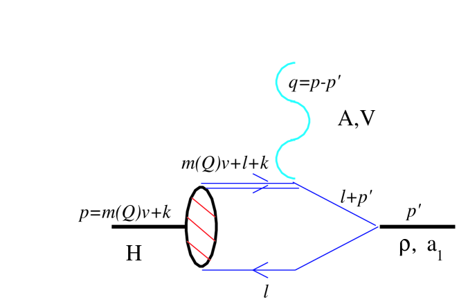
Figure 12: The CQM direct diagram.

The CQM expressions for the form factors derived by the direct diagrams calculations, are the following (here we can find the $\Omega_{i}$ expressions introduced in 4.2):

$$V^{D}(q^{2}) = -\frac{m_{\rho}^{2}}{f_{\rho}}\sqrt{\frac{Z_{H}}{m_{B}}}\left(\Omega_{1}-mZ\right)(m_{B}+m_{\rho})$$ (267)

$$A^{D}_{1}(q^{2}) = \frac{2m_{\rho}^{2}}{f_{\rho}}\sqrt{Z_{H}m_{B}}\frac{1}{m_{B}+m_{\rho}}$$ (268)

$$\left[(m^{2}+mm_{\rho}{\bar{\omega}})Z-{\bar{\omega}}m_{\rho}\Omega_{1}-m_{\rho}\Omega_{2}-2\Omega_{3}-\right.$$

$$\left.\Omega_{4}-\Omega_{5}-2{\bar{\omega}}\Omega_{6}\right]$$

$$A^{D}_{2}(q^{2}) = \frac{m_{\rho}^{2}}{f_{\rho}}\sqrt{\frac{Z_{H}}{m_{B}}}\left(mZ-\Omega_{1}-2\frac{\Omega_{6}}{m_{\rho}}\right)(m_{B}+m_{\rho})$$ (269)

$$A^{D}_{0}(q^{2}) = -\frac{m_{\rho}}{f_{\rho}}\sqrt{Z_{H}m_{B}}\left[\Omega_{1}\left(m_{\rho}{\bar{\omega}}+2m\frac{q^{2}}{m_{B}^{2}}-\frac{r_{1}}{m_{B}}\right)+m_{\rho}\Omega_{2}+\right.$$ (270)

$$\left.2\Omega_{3}+\Omega_{4}\left(1-2\frac{q^{2}}{m_{B}^{2}}\right)+\Omega_{5}+2\Omega_{6}\left(\bar{\omega}-\frac{r_{1}}{m_{B}m_{\rho}}\right)-\right.$$

$$\left.Z\left(m^{2}-m\frac{r_{1}}{m_{B}}+mm_{\rho}{\bar{\omega}}\right)\right],$$

where:

$${\bar{\omega}}=\frac{m_{B}^{2}+m_{\rho}^{2}-q^{2}}{2m_{B}m_{\rho}},$$ (271)

and:

$$r_{1}=\frac{m_{B}^{2}-q^{2}-m^{2}_{\rho}}{2}.$$ (272)

$Z$ and $\Omega_{j}$ are given in the Appendix. In the above expressions one must consider $\Delta_{1}=\Delta_{H}$, $\Delta_{2}=\Delta_{1}-m_{\rho}{\bar{\omega}}$, $x=m_{\rho}$.

The calculation for the $B\to a_{1}$ semileptonic transition proceeds in a similar way. We find:

$$A^{D}(q^{2}) = -\frac{m_{a}^{2}}{f_{a}}\sqrt{\frac{Z_{H}}{m_{B}}}\left(\Omega_{1}-mZ-\frac{2m}{m_{a}}\Omega_{2}\right)(m_{B}+m_{a})$$ (273)

$$V^{D}_{1}(q^{2}) = \frac{2m_{a}^{2}}{f_{a}}\sqrt{Z_{H}m_{B}}\frac{1}{m_{B}+m_{a}}$$ (274)

$$\left[(-m^{2}+mm_{a}\bar{\omega})Z+2m\Omega_{1}-\bar{\omega}m_{a}\Omega_{1}+\right.$$

$$\left.+(2m\bar{\omega}-m_{a})\Omega_{2}-2\Omega_{3}-\Omega_{4}-\Omega_{5}-2\bar{\omega}\Omega_{6}\right]$$

$$V^{D}_{2}(q^{2}) = \frac{m_{a}^{2}}{f_{a}}\sqrt{\frac{Z_{H}}{m_{B}}}\left(mZ-\Omega_{1}-2\frac{\Omega_{6}}{m_{a}}+2\frac{m}{m_{a}}\Omega_{2}\right)(m_{B}+m_{a})$$ (275)

$$V^{D}_{0}(q^{2}) = -\frac{m_{a}}{f_{a}}\sqrt{Z_{H}m_{B}}\left[\Omega_{1}\left(m_{a}\bar{\omega}+2m\frac{q^{2}}{m^{2}_{B}}-\frac{r_{1}^{\prime}}{m_{B}}-2m\right)+\right.$$ (276)

$$\left.\Omega_{2}\left(m_{a}+2m\frac{r_{1}^{\prime}}{m_{B}m_{a}}-2m\bar{\omega}\right)+2\Omega_{3}+\Omega_{4}\left(1-2\frac{q^{2}}{m^{2}_{B}}\right)+\Omega_{5}+\right.$$

$$\left.2\Omega_{6}\left(\bar{\omega}-\frac{r_{1}^{\prime}}{m_{B}m_{a}}\right)+Z\left(m^{2}+m\frac{r_{1}^{\prime}}{m_{B}}-mm_{a}\bar{\omega}\right)\right],$$

where now:

$${\bar{\omega}} = \frac{m_{B}^{2}+m_{a}^{2}-q^{2}}{2m_{B}m_{a}}$$ (277)

$$r_{1}^{\prime} = \frac{m_{B}^{2}-q^{2}-m^{2}_{a}}{2}.$$ (278)

	$V^{D}$	$A^{D}_{1}$	$A^{D}_{2}$	$A^{D}_{0}$	$A^{D}$	$V^{D}_{1}$	$V^{D}_{2}$	$V^{D}_{0}$
$F^{D}(0)$	$0.83$	$0.69$	$0.81$	$0.33$	$1.62$	$1.13$	$1.13$	$1.13$
$a_{F}$	$0.93$	$0$	$0.87$	$2.9$	$1.13$	$0.18$	$1.3$	$1.9$
$b_{F}$	$0.02$	$0$	$-0.17$	$2.6$	$0.12$	$0.04$	$3.8$	$0.93$

Table 8: CQM direct diagrams contributions to the form factors governing the semileptonic decays $B\to\rho$ and $B\to a_{1}$. The $F^{D}(0)$ values for the $B\to a_{1}$ transition must be multiplied with the normalization $0.25\leavevmode\nobreak\ {\rm GeV}^{2}/f_{a}$. The theoretical uncertainty is around $\pm 15\%$.

These results are amenable to a numerical analysis. Let’s consider the following parametrization:

$$F^{D}(q^{2})=\frac{F^{D}(0)}{1\leavevmode\nobreak\ -\leavevmode\nobreak\ a_{F}\left(\frac{q^{2}}{m_{B}^{2}}\right)+\leavevmode\nobreak\ b_{F}\left(\frac{q^{2}}{m_{B}^{2}}\right)^{2}},$$ (279)

for a generic direct form factor $F^{D}(q^{2})$; $a_{F},b_{F}$ have been obtained through a numerical analysis of the $q^{2}$ region going from $0$ to $q^{2}=16\leavevmode\nobreak\ {\rm GeV}^{2}$. Numerical values are listed in Table 8.

The form factors describing the $B\to a_{1}$ transition at $q^{2}=0$ are proportional to the normalization factor $(0.25\leavevmode\nobreak\ {\rm GeV}^{2}/f_{a})$ (recall the problems in the determination of $f_{a}$ mentioned in 4.2). These parameters are also affected by a theoretical uncertainty of about $15\%$.

5.3.2 Polar contributions

The polar contributions to the form factors come from those CQM diagrams in which the weak current is coupled to $B$ through an heavy meson intermediate state. In fig. 13 it is showed the related CQM loop diagram.

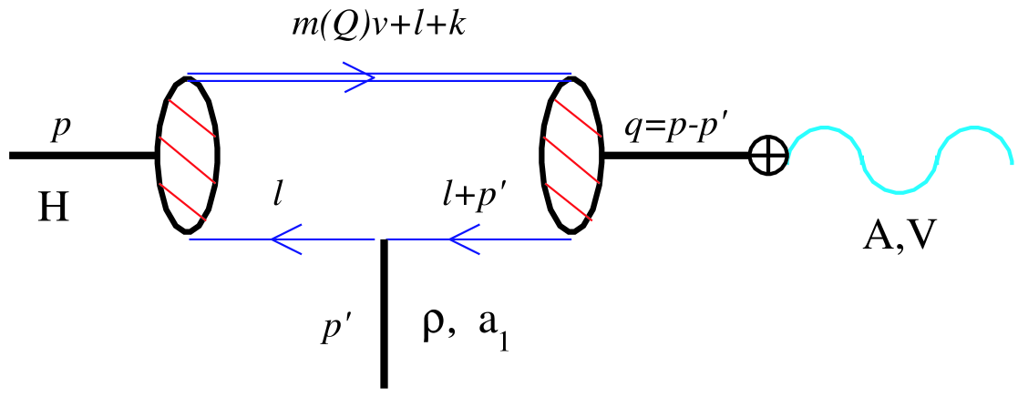
Figure 13: The CQM polar diagram.

The form factor will then have a typical polar behaviour:

$$F^{P}(q^{2})=\frac{F^{P}(0)}{1\leavevmode\nobreak\ -\leavevmode\nobreak\ \frac{q^{2}}{m_{P}^{2}}},$$ (280)

where $m_{P}$ is the mass of the intermediate virtual heavy meson state. This behaviour is certainly valid nearby the pole. Let’s assume that it is valid all over the $q^{2}$ range that we want to explore, i.e., also for small $q^{2}$ values. This hypothesis is a good one for the form factors $A_{1}^{P},A_{2}^{P}$ (where the superscript $P$ indicates that they are derived from the polar diagram), since they are numerically small, with respect to $A_{1}^{D},A_{2}^{D}$, in the range of small $q^{2}$ values. Things are different for $A_{0}^{P}(q^{2})$ and $V_{0}^{P}(q^{2})$, we shall come back on this point later.

Using the strong couplings calculated in 4.2 and the leptonic decay constants obtained in 5.1, we can calculate the different contributions to $F^{P}(0)$. As for the semileptonic transition $B\to\rho$, they are [39]:

$$V^{P}(0) = -\sqrt{2}g_{V}\lambda{\hat{F}}\frac{m_{B}+m_{\rho}}{m_{B}^{3/2}}$$ (281)

$$A^{P}_{1}(0) = \frac{\sqrt{2m_{B}}g_{V}{\hat{F}}^{+}}{m_{B_{0}}(m_{B}+m_{\rho})}(\zeta-2\mu{\bar{\omega}}m_{\rho})$$ (282)

$$A^{P}_{2}(0) = -\sqrt{2}g_{V}\mu{\hat{F}}^{+}\frac{\sqrt{m_{B}}(m_{B}+m_{\rho})}{m_{B_{0}}^{2}},$$ (283)

where ${\bar{\omega}}=m_{B}/(2m_{\rho})$, while $\lambda,\mu,\beta,\zeta$ and $g_{V}$ have been defined and calculated in 4.2. As for $A^{P}_{0}(q^{2})$, we have to impose the condition (264); a possible choice is:

$$A^{P}_{0}(q^{2})=A^{P}_{3}(0)+g_{V}\beta{\hat{F}}\frac{1}{m_{\rho}\sqrt{2m_{B}}}\frac{q^{2}}{m^{2}_{B}-q^{2}}.$$ (284)

Let’s discuss this equation in greater detail. The amplitude for the semileptonic process $B\to\rho$ can be written, see fig. 14, in the following way:

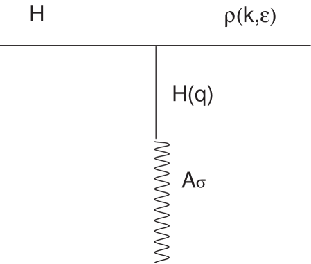
Figure 14: The polar diagram at the level of meson interactions.

$${\rm Amp}(B\to\rho) = \langle{\rm VAC}|A^{\sigma}|H\rangle\frac{i}{q^{2}-m_{B}^{2}}\langle H(q)\rho(k,\epsilon)|i{\cal L}|H\rangle$$ (285)

$$= i\frac{{\hat{F}}}{\sqrt{m_{B}}}q^{\sigma}\frac{i}{q^{2}-m_{B}^{2}}C(\epsilon^{*}\cdot q),$$

where $H$ is the $0^{-}$ state. We have used eq. (214) and the interaction Lagrangian term multiplied by $\beta$ in (190). It is easy to find that:

$$C=i\sqrt{2}g_{V}\beta,$$ (286)

therefore:

$${\rm Amp}(B\to\rho)=i\sqrt{2}g_{V}\beta\frac{{\hat{F}}}{\sqrt{m_{B}}}\frac{(\epsilon^{*}\cdot q)}{q^{2}}\frac{q^{2}}{q^{2}-m_{B}^{2}}.$$ (287)

Equation (287) should be compared with eq. (5.3):

$$i2m_{\rho}[A_{3}^{P}(q^{2})-A_{0}^{P}(q^{2})]\frac{(\epsilon^{*}\cdot q)}{q^{2}}.$$ (288)

What then follows is (284).

As for the semileptonic transition $B\to a_{1}$, one has:

$$A^{P}(0) = -\sqrt{2}g_{A}\lambda_{A}{\hat{F}}^{+}\frac{m_{B}+m_{a}}{m_{B}^{3/2}}$$ (289)

$$V^{P}_{1}(0) = \frac{\sqrt{2m_{B}}g_{A}{\hat{F}}}{m_{B}(m_{B}+m_{a})}(\zeta_{A}-2\mu_{A}{\bar{\omega}}m_{a})$$ (290)

$$V^{P}_{2}(0) = -\sqrt{2}g_{A}\mu_{A}{\hat{F}}\frac{\sqrt{m_{B}}(m_{B}+m_{a})}{m_{B}^{2}},$$ (291)

where ${\bar{\omega}}=m_{B}/(2m_{a})$. A similar reasoning as the one made before can be applied for $V^{P}_{0}(q^{2})$:

$$V^{P}_{0}(q^{2})=V^{P}_{3}(0)+g_{A}\beta_{A}{\hat{F}}^{+}\frac{1}{m_{a}\sqrt{2m_{B}}}\frac{q^{2}}{m^{2}_{B_{0}}-q^{2}}.$$ (292)

One should note that, if we do the hypothesis of massless leptons in the final state, these $V_{0}^{P}$ and $A_{0}^{P}$ form factors do not contribute to the process width and can therefore be ignored.

Numerical results have been given in Table 9 together with the polar masses. A theoretical uncertainty of $\pm 15\%$ is estimated. In fig. 15 we plot $A_{1}$ and $A_{2}$, while in fig. 16 the form factors $A$, $V_{1}$ and $V_{2}$ are showed together. We don’t plot $V(q^{2})$ in fig. 15 since the theoretical prediction for this value is affected by a large uncertainty. Plots do not account of the errors given in Tables.

	$V^{P}$	$A^{P}_{1}$	$A^{P}_{2}$	$A^{P}_{0}$	$A^{P}$	$V^{P}_{1}$	$V^{P}_{2}$	$V^{P}_{0}$
$F^{P}(0)$	$-0.84$	$-0.11$	$-0.15$	$-0.019$	$-1.48$	$-0.32$	$-0.57$	$0.07$
$m_{P}$	$5.3$	$5.5$	$5.5$	$-$	$5.5$	$5.3$	$5.3$	$-$

Table 9: Polar form factors for $B\to\rho$ and $B\to a_{1}$ semileptonic decays. Polar masses have GeV dimensions. The $F^{P}(0)$ values for the $B\to a_{1}$ transition should be multiplied by the normalization factor $(0.25\leavevmode\nobreak\ {\rm GeV}^{2}/f_{a})$. The theoretical uncertainty amounts to $\pm 15\%$.

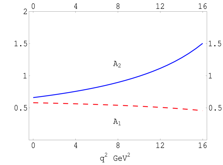
Figure 15: Form factors $A_{1}$ and $A_{2}$ for the semileptonic decay $B\to\rho$.

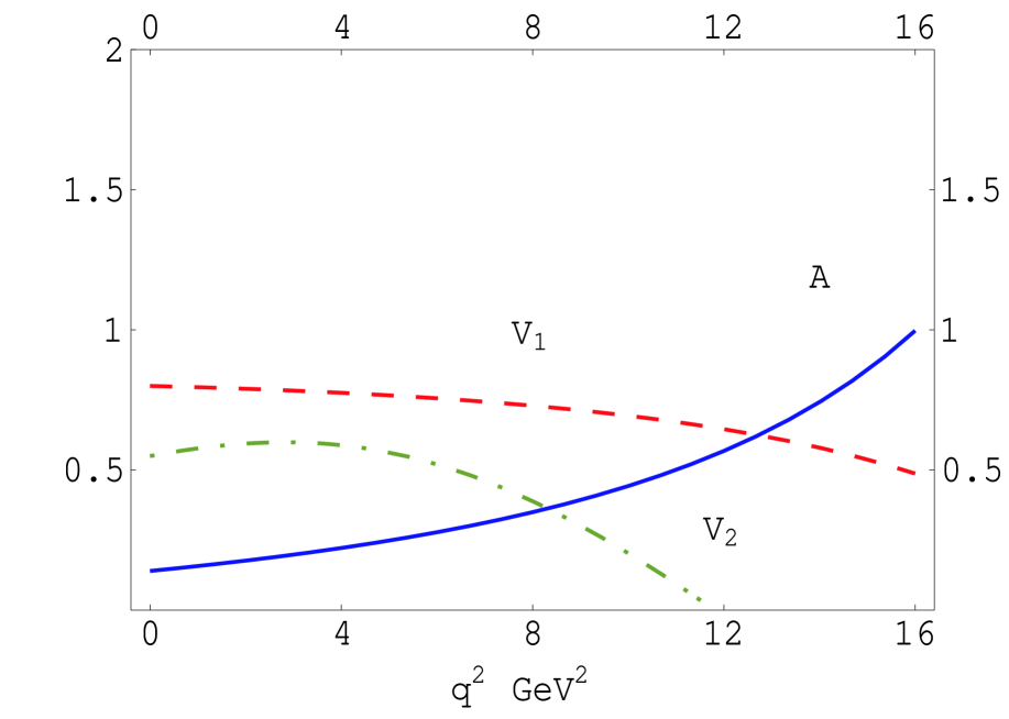
Figure 16: Form factors $A$, $V_{1}$ and $V_{2}$ for the semileptonic decay $B\to a_{1}$.

5.3.3 Branching ratios and widths

Using the numerical values given in the Tables, one can compute semileptonic branching ratios and widths. First of all let’s compare CQM results for $B\to\rho$ with what is obtained by other methods. In Table 10 we show the form factors obtained summing up direct and polar contributions:

$$F(q^{2})=F^{D}(q^{2})+F^{P}(q^{2}).$$ (293)

Here the CQM results are compared with those obtained by other approaches. In particular, I would comment on the method followed in [92]. The idea is that of describing the heavy meson field $H$ as an effective interpolating field given by the operator product of the two constituent quark projectors times a momentum space wave function, solution of the Bethe-Salpeter equation for the Richardson potential (having the confining behavior at large distances and the Coulombic one at short distances). With such a description of the heavy field, the calculation of the correlator $\langle{\rm VAC}|T\{J_{1}JJ_{2}\}|{\rm VAC}\rangle$, typical of potential models, where $J_{1}$ and $J_{2}$ are the effective interpolating currents of the light mesons in the final state, $M_{1}$ and $M_{2}$, while $J$ is the current of the process, is substituted by the calculation of the amplitude $\langle M_{1}M_{2}|J|H\rangle$. This approach gives results for the semileptonic decays $B\to\rho\ell\nu$ and $B\to K^{*}\ell^{+}\ell^{-}$ that are in quite good agreement with those obtained by lattice and QCD sum rules (in the $q^{2}$ region where these latter methods are predictive).

As one can see, the CQM result obtained for $V^{\rho}(q^{2})$ is affected by a large theoretical uncertainty since it turns out to be the sum of two numerical values almost identical in magnitude, but opposite in sign. Aside from this problem, the CQM values are generally in good agreement with those found by QCD sum rules; with respect to other approaches they show to be systematically higher.

	CQM	PM[92]	LCSR [93]	SR [94]	LLCSR [95]
$V^{\rho}(0)$	$-0.01\pm 0.25$	$0.45\leavevmode\nobreak\ \pm\leavevmode\nobreak\ 0.11$	$0.34\leavevmode\nobreak\ \pm\leavevmode\nobreak\ 0.05$	$0.6\leavevmode\nobreak\ \pm\leavevmode\nobreak\ 0.2$	$0.35^{+0.06}_{-0.05}$
$A_{1}^{\rho}(0)$	$0.58\pm 0.10$	$0.27\leavevmode\nobreak\ \pm\leavevmode\nobreak\ 0.06$	$0.26\leavevmode\nobreak\ \pm\leavevmode\nobreak\ 0.04$	$0.5\leavevmode\nobreak\ \pm\leavevmode\nobreak\ 0.1$	$0.27^{+0.05}_{-0.04}$
$A_{2}^{\rho}(0)$	$0.66\pm 0.12$	$0.26\leavevmode\nobreak\ \pm\leavevmode\nobreak\ 0.05$	$0.22\leavevmode\nobreak\ \pm\leavevmode\nobreak\ 0.03$	$0.4\leavevmode\nobreak\ \pm\leavevmode\nobreak\ 0.2$	$0.26^{+0.05}_{-0.03}$
$A_{0}^{\rho}(0)$	$0.33\pm 0.05$	$0.29\leavevmode\nobreak\ \pm\leavevmode\nobreak\ 0.09$		$0.24\pm 0.02$	$0.30^{+0.06}_{-0.04}$

Table 10: Form factors for the $B\to\rho$ transition at $q^{2}=0$. The CQM results are compared with those obtained by other theoretical approaches: a potential model (PM), light cone sum rules (LCSR), QCD sum rules (SR), lattice calculations with (SR), i.e. (LLCSR). The large theoretical uncertainty on $V^{\rho}(0)$ is due to the strong cancellation between direct and polar contributions.

Using $V_{ub}=0.0032$ and $\tau_{B}=1.56\times 10^{-12}$ s, we obtain for $B\to\rho\ell\nu$:

$${\cal B}(\bar{B}^{0}\to\rho^{+}\ell\nu) = (2.5\pm 0.8)\times 10^{-4}$$

$$\Gamma_{0}(\bar{B}^{0}\to\rho^{+}\ell\nu) = (4.4\pm 1.3)\times 10^{7}\;s^{-1}$$

$$\Gamma_{+}(\bar{B}^{0}\to\rho^{+}\ell\nu) = (7.1\pm 4.5)\times 10^{7}\;s^{-1}$$

$$\Gamma_{-}(\bar{B}^{0}\to\rho^{+}\ell\nu) = (5.5\pm 3.7)\times 10^{7}\;s^{-1}$$

$$(\Gamma_{+}+\Gamma_{-})(\bar{B}^{0}\to\rho^{+}\ell\nu) = (1.26\pm 0.38)\times 10^{8}\;s^{-1},$$ (294)

where $\Gamma_{0}$, $\Gamma_{+}$, $\Gamma_{-}$ are referred to the three helicity states of $\rho$. This branching ratio is evidently consistent with the experimental one (213).

The reported results may be computed for different $V_{ub}$ values just multiplying by $|V_{ub}/0.0032|^{2}$ and choosing a particular $V_{ub}$. The same holds for $\tau_{B}$ (sec) multiplying it by $\tau_{B}/(1.56\times 10^{-12})$.

A discussion on the theoretical uncertainty of these values is in order. The large error on $V^{\rho}(0)$ reflects in the determination of $\Gamma_{+}$ and $\Gamma_{-}$, but it doesn’t affect $\Gamma_{0}$ and has only a small effect on the branching ratio. Theoretical uncertainties for $A_{1}^{\rho}(0)$ and $A_{2}^{\rho}(0)$ are probably related. The theoretical error on widths comes from the sum in quadrature of the error on $V^{\rho}(0)$ and a $\pm 15\%$ error common to $A_{1}^{\rho}(0)$ and $A_{2}^{\rho}(0)$.

Let’s turn now to the semileptonic channel $B\to a_{1}\ell\nu$. CQM predictions for it are the following:

$${\cal B}(\bar{B}^{0}\to a_{1}^{+}\ell\nu) = (8.4\pm 1.6)\times 10^{-4}$$

$$\Gamma_{0}(\bar{B}^{0}\to a_{1}^{+}\ell\nu) = (4.0\pm 0.7)\times 10^{8}\;s^{-1}$$

$$\Gamma_{+}(\bar{B}^{0}\to a_{1}^{+}\ell\nu) = (4.6\pm 0.9)\times 10^{7}\;s^{-1}$$

$$\Gamma_{-}(\bar{B}^{0}\to a_{1}^{+}\ell\nu) = (0.98\pm 0.18)\times 10^{8}\;s^{-1},$$ (295)

where $\Gamma_{0}$, $\Gamma_{+}$, $\Gamma_{-}$ label the three helicity states of $a_{1}$.

In the determination of these decay widths we have included only the uncertainty arising from $f_{a}$. Lower values correspond to $f_{a}=0.30\leavevmode\nobreak\ {\rm GeV}^{2}$, while higher values correspond to $f_{a}=0.25\leavevmode\nobreak\ {\rm GeV}^{2}$. The theoretical errors arising from the form factors at $q^{2}=0$ are difficult to estimate reliably and are not included in this analysis. We can guess that the theoretical uncertainty is larger at least by a factor of two.

CQM predicts a branching ratio for the $\bar{B}^{0}\to a_{1}^{+}\ell\nu$ decay higher than the branching ratio for $\bar{B}^{0}\to\rho^{+}\ell\nu$ and this analysis shows that $\bar{B}^{0}\to a_{1}^{+}\ell\nu$ could be responsible for almost the $50\%$ of the semileptonic channel $B\to X_{u}\ell\nu$; the $B\to\rho\ell\nu$ takes another $15\%$.

The form factor $A$ suffers for an analogous cancellation problem as $V$. The analysis of Aliev and Savci [71], based on the QCD sum rules method, gives a value for $A$ that is five times smaller than the CQM predicted one (with the sign reversed, but this is because of a different overall phase definition of the hadronic matrix elements).

5.4 $B\to\pi\ell\nu$

The semileptonic $B\to\pi\ell\nu$ channel is of crucial interest for the evaluation of the CKM matrix element $V_{ub}$ and it has been widely investigated in literature, see the reviews [35] and [96].

CQM allows for a simple determination of the already known leading terms in the soft pion emission limit and of a new sub-leading contribution computed beyond the soft pion limit approximation, i.e., through the technique discussed in 4.1.2.

Let’s then write the weak current matrix element for the semileptonic transition amplitude $B\to\pi$ [35]:

$$\langle\pi(q_{\pi})|V^{\mu}(q)|B(p)\rangle = \left[(p+q_{\pi})^{\mu}+\frac{m_{\pi}^{2}-m_{B}^{2}}{q^{2}}q^{\mu}\right]\;F_{1}(q^{2})$$ (296)

$$- \left[\frac{m_{\pi}^{2}-m_{B}^{2}}{q^{2}}q^{\mu}\right]\;F_{0}(q^{2}),$$

where $F_{1}(0)=F_{0}(0)$.

5.4.1 The non derivative contribution

The diagram in fig. 17 shows a non derivative coupling of the pion to the $B$ meson and to the weak current. To obtain the contribution to the form factors deriving from the diagram in fig. 17, one has to expand $\chi=\xi q$, defined in 3.1.2, up to the first order in $\pi$, neglecting the term of order zero. In so far we have always considered $\chi=q$, truncating the expansion at order zero.

Of course the diagram in fig. 17 produces a result proportional to the leptonic decay constant of $B$, as one can easily see comparing fig. 17 with fig. 9.

On the other hand, the diagram in fig. 17 makes sense only for very small $q_{\pi}$, i.e., in the limit in which almost the entire incoming meson momentum is brought away by the weak current.

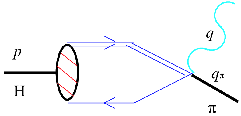
Figure 17: “Callan-Treiman” contribution to the form factors of the $B\to\pi$ semileptonic decay.

We therefore obtain [41]:

$$F_{0}^{\rm ND} = \frac{f_{B}}{f_{\pi}}$$ (297)

$$F_{1}^{\rm ND} = \frac{f_{B}}{2f_{\pi}},$$ (298)

where $f_{B}$ was defined in (218).

5.4.2 The polar contribution

Consider now a diagram of the kind of that given in fig. 13 where, instead of $\rho$ or $a_{1}$, one must consider the pion attached, through a derivative coupling, to the light quarks. The intermediate meson state can be a $1^{-}$ state, belonging to the $H$ multiplet, or a $0^{+}$ state, belonging to the $S$ multiplet. The latter case is less important since it produces only a small correction to the chiral limit.

Consider the case in which the intermediate meson state is $1^{-}$. Having in mind fig. 13, we expect a contribution proportional to $g\hat{F}$, where $g$, the strong coupling constant $HH\pi$, has been calculated through CQM in in 4.1.1. The following contribution to $F_{1}$ has been obtained [35, 37]:

$$F_{1}^{\rm Pol}(q^{2})=\frac{\hat{F}g}{f_{\pi}\sqrt{m_{B}}}\frac{1}{1-q^{2}/m_{B^{*}}^{2}}.$$ (299)

If instead the polar meson is $0^{+}$, one has:

$$F_{0}^{\rm Pol}(q^{2})=\frac{1}{m_{B}^{2}-m_{\pi}^{2}}\left(\frac{hm_{\pi}\sqrt{m_{B}}{\hat{F}}^{+}}{f_{\pi}}\right)\frac{1}{1-q^{2}/m_{B^{**}}^{2}},$$ (300)

where $h$ is the coupling constant $HS\pi$ discussed in 4.1.2 and by $B^{**}$ we mean the $0^{+}$ state. The linear dependence of (300) on $m_{\pi}$ makes this term not relevant in the chiral limit.

The polar form factors (299, 300) are reliable near the poles, i.e., for $q^{2}\simeq m_{B}$. We will discuss later about one way to extrapolate these results to a wider $q^{2}$ range. Numerically, if one uses the CQM results obtained in so far, one finds:

$$F_{1}^{\rm Pol}(0) = 0.52\pm 0.01$$ (301)

$$F_{0}^{\rm Pol}(0) = 0.012\pm 0.001.$$ (302)

5.4.3 The direct contribution

The contributions discussed above are well known in literature. CQM predicts the existence of a new contribution due to a diagram of the kind of that depicted in fig. 12 where the pion couples directly to $B$ and to the weak current. This contribution differs from the non derivative one (ND), since it is derivative, and from the polar (which instead is derivative), since it doesn’t contain couplings to resonances.

The evaluation of these diagrams proceeds following the rules we have already discussed many times. The result is:

$$F_{1}^{\rm Dir}(q^{2}) = \frac{2}{f_{\pi}}\sqrt{\frac{Z_{H}}{m_{H}}}\left[q_{\pi}(C-mA)+m_{H}\;B\right]$$ (303)

$$F_{0}^{\rm Dir}(q^{2}) = \frac{2}{f_{\pi}}\sqrt{\frac{Z_{H}}{m_{H}}}\left[\left(1-\frac{q^{2}}{m_{\pi}^{2}-m_{B}^{2}}\right)q_{\pi}(C-mA)\right.$$ (304)

$$+ \left.m_{H}\;B\left(1+\frac{q^{2}}{m_{\pi}^{2}-m_{B}^{2}}\right)\right],$$

where:

$$A = \frac{1}{2q_{\pi}}(I_{3}(\Delta_{H}-q_{\pi})-I_{3}(\Delta_{H}))$$ (305)

$$B = mA-m^{2}Z(\Delta_{H})$$ (306)

$$C = \frac{1}{2q_{\pi}}(\Delta_{H}I_{3}(\Delta_{H})-(\Delta_{H}-q_{\pi})I_{3}(\Delta_{H}-q_{\pi})).$$ (307)

Here we have used the notation $q_{\pi}^{\mu}=(q_{\pi},0,0,q_{\pi})$, while $Z$ is given in the Appendix. Observe that the dependence of (303) and (304) on $q^{2}$ is due to the fact that:

$$q_{\pi}=(m_{B}^{2}-q^{2})/2m_{B}.$$ (308)

Numerically we find:

$$F_{1}^{\rm Dir}(q^{2}=0)=F_{0}^{\rm Dir}(q^{2}=0)=0.13\pm 0.05.$$ (309)

The error made in the numeric evaluation is due to the variation of $\Delta_{H}$ in the range $0.3-0.5$ GeV. The direct diagram contribution induces a correction to the form factors that ranges from $10\%$ to $30\%$ depending on $q^{2}$.

Since the three contributions to $F_{0}$ and $F_{1}$ are independent, one can sum them up with the following result:

$$\hat{F_{j}}(q^{2})=\frac{f_{B}}{(j+1)f_{\pi}}+F_{j}^{\rm Dir}(q^{2})+\frac{F_{j}^{\rm Pol}(0)}{1-q^{2}/m^{2}_{j}},$$ (310)

where $m_{1}=m_{B^{*}}$, $m_{0}=m_{B^{**}}$ and we have indicated the total form factor as $\hat{F}$. $\hat{F}$ is the correct total form factor only when we are at the maximum value of $q^{2}$, i.e., $q^{2}\simeq m_{B}^{2}=q_{0}^{2}$. The $\hat{F_{j}}$ form factors could be seen as the first terms in an expansion where higher terms are characterized by an increasing number of derivatives of the pion field. These terms are subleading only when $q^{2}$ is high.

Let’s try to extrapolate to small $q^{2}$ values using the auxiliary functions $G_{j}(q^{2})$:

$$F_{j}(q^{2})=\hat{F_{j}}(q^{2})G_{j}(q^{2}),$$ (311)

where $j\in(0,1)$. This parameterization must satisfy the condition:

$$G_{j}(q_{0}^{2})=1,$$ (312)

since $q^{2}\simeq q_{0}^{2}$ is the region where $\hat{F_{j}}$ are better approximating the $F_{j}$.

Since ${F_{1}}(0)={F_{0}}(0)$, the following condition must hold:

$$\hat{F_{1}}(0)G_{1}(0)=\hat{F_{0}}(0)G_{0}(0).$$ (313)

It is reasonable to assume that the corrections to $G_{j}(q^{2})\equiv 1$ come from terms in which one has one more derivative of the pion field. Let’s put:

$$G_{j}(q^{2})=1+\frac{E_{\pi}}{\alpha_{j}\Lambda_{\chi}}=1+\frac{(q_{\pi}\cdot p)}{\alpha_{j}m_{B}\Lambda_{\chi}},$$ (314)

where $E_{\pi}$ is the pion energy in the frame where $B$ is at rest, while $\alpha_{j}$ are free parameters. Moreover, since (314) is equivalent to:

$$G_{j}(q^{2})=1+\frac{q^{2}-m_{B}^{2}}{2m_{B}\Lambda_{\chi}\alpha_{j}},$$ (315)

the condition (312) is automatically satisfied. Equation (313) implies that $\alpha_{0}$ and $\alpha_{1}$ are related according to:

$$\frac{2\Lambda_{\chi}\alpha_{1}}{m_{B}}=1-\left(1-\frac{m_{B}}{2\Lambda_{\chi}\alpha_{0}}\right)\frac{\hat{F_{0}}(0)}{\hat{F_{1}}(0)}.$$ (316)

It is not possible to fix the $\alpha$ constants only from experimental data, therefore we need to refer to other theoretical evaluations in literature. Quark models, [97]-[99], predict $F_{0}(0)=0.20-0.50$, with the exception of [100], which gives a value of $F_{0}(0)=0.09$. QCD and factorization combined give $F_{0}(0)=0.33$ [101], while chiral effective theory and HQET combined give $F_{0}(0)=0.38$ [35]. QCD sum rules give $F_{0}(0)=0.25-0.40$ [102]-[103] and some lattice QCD computations give $F_{0}(0)=0.27-0.35$ [104]-[106].

Let’s use, as an input parameter, the result obtained with QCD sum rules in [107], according to which $F_{0}(0)=0.30\pm 0.04$. In so doing, one finds $\alpha_{0}=3.6$. An $\alpha_{0}>1$ suggests that the energy scale controlling the expansion (314) is not $\Lambda_{\chi}\simeq 1$ GeV, but larger. At this point one has to remind that the first term in (314) describes the situation in which $q^{2}\simeq q_{0}^{2}$ while, in the corrections depending on the pion momentum, we could have $q_{\pi}$ values higher than expected, due to an effective expansion scale $\alpha\Lambda_{\chi}>\Lambda_{\chi}$. In such a way we can extend to small $q^{2}$ values the range of validity of the form factor expressions.

In Table 11 we show, for some $q^{2}$ values, the two form factors $F_{1}$ and $F_{0}$ also containing the CQM correction. On the obtained results one can compute the error due to a variation of $\alpha_{0}$ in the range $(2.9,3.6,4.3)$. What can be read off from Table 11 is that CQM is in good agreement with the results obtained by other methods. This also means that the CQM deviations from the dominating contributions (the Callan-Treiman and the polar one), due to the direct contributions, are not strong enough to modify qualitatively the polar behaviour of the form factors predicted by the chiral effective theory.

$q^{2}$	14.9 GeV2	17.2 GeV2	20 GeV2	26.4 GeV2
CQM
$F_{1}^{B\pi}$	$1.58^{+0.28}_{-0.52}$	$2.06^{+0.27}_{-0.50}$	$2.96^{+0.26}_{-0.47}$	$13.78^{+0.13}_{-0.31}$
$F_{0}^{B\pi}$	$0.59^{+0.10}_{-0.18}$	$0.62^{+0.08}_{-0.14}$	$0.65^{+0.05}_{-0.10}$	$0.83\pm 0.01$
IS [108]
$F_{1}^{B\pi}$	0.83	0.96	1.19	3.14
$F_{0}^{B\pi}$	0.48	0.48	0.48	0.47
GNS [98]
$F_{1}^{B\pi}$	0.82	1.05	1.45	2.31
$F_{0}^{B\pi}$	0.38	0.40	0.40	0.07
LNS [99]
$F_{1}^{B\pi}$	0.53	0.57	–	–
$F_{0}^{B\pi}$	0.69	0.76	–	–
Ball [103]
$F_{1}^{B\pi}$	$0.85\pm 0.15$	$1.1\pm 0.2$	1.6	–
$F_{0}^{B\pi}$	$0.5\pm 0.1$	$0.55\pm 0.15$	0.7	–
Lattice (UKQCD) [106]
$F_{1}^{B\pi}$	$0.85\pm 0.20$	$1.10\pm 0.27$	$1.72\pm 0.50$	–
$F_{0}^{B\pi}$	$0.46\pm 0.10$	$0.49\pm 0.10$	$0.56\pm 0.12$	–

Table 11: Form factors $F_{1}$ and $F_{0}$ predicted by CQM at high $q^{2}$ (near $q^{2}_{max}\simeq 26.4{\rm GeV}^{2}$) and comparison with other theoretical evaluations. The error quoted for CQM results is due to a variation of $20\%$ in the parameter controlling the evolution from higher to lower $q^{2}$ values, where the results are less reliable. IS, GNS and LNS (from author names), are quark models, while the Ball’s paper makes use of light cone QCD sum rules.

6 Appendix

This Appendix is completely devoted to the $I_{i}$ integrals used in the text and to their linear combinations arising in CQM applications. These integrals have been computed adopting the proper time regularization prescription discussed in 3.1.3. The analytical expressions here listed, have been numerically treated using Mathematica 3.0. Everywhere $N_{c}=3$ is meant.

$$I_{0}(\Delta) = \frac{iN_{c}}{16\pi^{4}}\int^{\mathrm{reg}}\frac{d^{4}k}{(v\cdot k+\Delta+i\epsilon)}$$ (317)

$$= {N_{c}\over{16\,{{\pi}^{{3/2}}}}}\int_{1/{{{\Lambda}^{2}}}}^{1/{{{\mu}^{2}}}}{ds\over{s^{3/2}}}\;e^{-s({m^{2}}-{{\Delta}^{2}})}\left({3\over{2\,s}}+{m^{2}}-{{{\Delta}}^{2}}\right)[1+{\mathrm{erf}}(\Delta\sqrt{s})]$$

$$- \Delta{{N_{c}m^{2}}\over{16\pi^{2}}}\Gamma\left(-1,{{{m^{2}}}\over{{{\Lambda}^{2}}}},{{{m^{2}}}\over{{{\mu}^{2}}}}\right)$$

$$I_{1} = \frac{iN_{c}}{16\pi^{4}}\int^{reg}\frac{d^{4}k}{(k^{2}-m^{2})}={{N_{c}m^{2}}\over{16\pi^{2}}}\Gamma\left(-1,{{{m^{2}}}\over{{{\Lambda}^{2}}}},{{{m^{2}}}\over{{{\mu}^{2}}}}\right)$$ (318)

$$I_{1}^{\prime} = \frac{iN_{c}}{16\pi^{4}}\int^{\mathrm{reg}}d^{4}k\frac{k^{2}}{(k^{2}-m^{2})}={{N_{c}m^{4}}\over{8\pi^{2}}}\Gamma\left(-2,{{{m^{2}}}\over{{{\Lambda}^{2}}}},{{{m^{2}}}\over{{{\mu}^{2}}}}\right)$$ (319)

$$I_{2} = -\frac{iN_{c}}{16\pi^{4}}\int^{\mathrm{reg}}\frac{d^{4}k}{(k^{2}-m^{2})^{2}}=\frac{N_{c}}{16\pi^{2}}\Gamma\left(0,\frac{m^{2}}{\Lambda^{2}},\frac{m^{2}}{\mu^{2}}\right)$$ (320)

$$I_{3}(\Delta) = -\frac{iN_{c}}{16\pi^{4}}\int^{\mathrm{reg}}\frac{d^{4}k}{(k^{2}-m^{2})(v\cdot k+\Delta+i\epsilon)}$$ (321)

$$= {N_{c}\over{16\,{{\pi}^{{3/2}}}}}\int_{1/{{\Lambda}^{2}}}^{1/{{\mu}^{2}}}{ds\over{s^{3/2}}}\;e^{-s({m^{2}}-{{\Delta}^{2}})}\;\left(1+{\mathrm{erf}}(\Delta\sqrt{s})\right)$$

$$I_{4}(\Delta) = \frac{iN_{c}}{16\pi^{4}}\int^{\mathrm{reg}}\frac{d^{4}k}{(k^{2}-m^{2})^{2}(v\cdot k+\Delta+i\epsilon)}$$ (322)

$$= \frac{N_{c}}{16\pi^{3/2}}\int_{1/\Lambda^{2}}^{1/\mu^{2}}\frac{ds}{s^{1/2}}\;e^{-s(m^{2}-\Delta^{2})}\;[1+{\mathrm{erf}}(\Delta\sqrt{s})]\leavevmode\nobreak\ .$$

In these equations,

$$\Gamma(\alpha,x_{0},x_{1})=\int_{x_{0}}^{x_{1}}dt\;e^{-t}\;t^{\alpha-1},$$ (323)

is the incomplete gamma function, while erf is the error function defined by:

$${\rm erf}(z)=\frac{2}{\sqrt{\pi}}\int_{0}^{z}dxe^{-x^{2}}.$$ (324)

Let us now introduce:

$$\sigma(x,\Delta_{1},\Delta_{2},\omega)={{{\Delta_{1}}\,\left(1-x\right)+{\Delta_{2}}\,x}\over{{\sqrt{1+2\,\left(\omega-1\right)\,x+2\,\left(1-\omega\right)\,{x^{2}}}}}}$$ (325)

$$I_{5}(\Delta_{1},\Delta_{2},\omega) = \frac{iN_{c}}{16\pi^{4}}\int^{\mathrm{reg}}\frac{d^{4}k}{(k^{2}-m^{2})(v\cdot k+\Delta_{1}+i\epsilon)(v^{\prime}\cdot k+\Delta_{2}+i\epsilon)}$$ (326)

$$= \int_{0}^{1}dx\frac{1}{1+2x^{2}(1-\omega)+2x(\omega-1)}\times$$

$$\Big{[}\frac{6}{16\pi^{3/2}}\int_{1/\Lambda^{2}}^{1/\mu^{2}}ds\leavevmode\nobreak\ \sigma\;e^{-s(m^{2}-\sigma^{2})}\;s^{-1/2}\;(1+{\mathrm{erf}}(\sigma\sqrt{s}))+$$

$$\frac{6}{16\pi^{2}}\int_{1/\Lambda^{2}}^{1/\mu^{2}}ds\;e^{-s(m^{2}-2\sigma^{2})}\;s^{-1}\Big{]}$$

$$I_{6}(\Delta_{1},\Delta_{2},\omega) = \frac{iN_{c}}{16\pi^{4}}\int^{\mathrm{reg}}\frac{d^{4}k}{(v\cdot k+\Delta_{1}+i\epsilon)(v^{\prime}\cdot k+\Delta_{2}+i\epsilon)}$$ (327)

$$= I_{1}\int_{0}^{1}dx\frac{\sigma}{1+2x^{2}(1-\omega)+2x(\omega-1)}$$

$$- \frac{N_{c}}{16\pi^{3/2}}\int_{0}^{1}dx\frac{1}{1+2x^{2}(1-\omega)+2x(\omega-1)}\times$$

$$\int_{1/\Lambda^{2}}^{1/\mu^{2}}\frac{ds}{s^{3/2}}e^{-s(m^{2}-\sigma^{2})}\Big{\{}\sigma[1+{\mathrm{erf}}(\sigma\sqrt{s})]\cdot[1+2s(m^{2}-\sigma^{2})]$$

$$+ 2{\sqrt{\frac{s}{\pi}}}e^{-s\sigma^{2}}\left[\frac{3}{2s}+(m^{2}-\sigma^{2})\right]\Big{\}}.$$

In the $\tau_{1/2,3/2}$ form factor determination, the following expressions are needed:

$$S(\Delta_{1},\Delta_{2},\omega) = \Delta_{1}\,I_{3}(\Delta_{2})+\omega\,\left(I_{1}+\Delta_{2}\,I_{3}(\Delta_{2})\right)+{{\Delta_{1}}^{2}}\,I_{5}(\Delta_{1},\Delta_{2},\omega)$$

$$T(\Delta_{1},\Delta_{2},\omega) = {m^{2}}\,I_{5}(\Delta_{1},\Delta_{2},\omega)+I_{6}(\Delta_{1},\Delta_{2},\omega)$$

$$U(\Delta_{1},\Delta_{2},\omega) = I_{1}+\Delta_{2}\,I_{3}(\Delta_{2})+\Delta_{1}\,I_{3}(\Delta_{1})+\Delta_{2}\,\Delta_{1}\,I_{5}(\Delta_{1},\Delta_{2},\omega).$$ (328)

Here are listed the integral $Z$, introduced in 4.1.1, and all the auxiliary combinations used during the study of $T\to H\pi$, $S\to H\pi$ processes:

$$Z(\Delta) = \frac{iN_{c}}{16\pi^{4}}\int^{\mathrm{reg}}\frac{d^{4}k}{(k^{2}-m^{2})[(k+q)^{2}-m^{2}](v\cdot k+\Delta+i\epsilon)}$$ (329)

$$= \frac{N_{c}}{16\pi^{3/2}}\int_{1/\Lambda^{2}}^{1/\mu^{2}}\frac{ds}{s^{1/2}}e^{-sm^{2}}\int_{0}^{1}dxe^{s\Delta^{2}(x)}[1+{\mathrm{erf}}(\Delta(x)\sqrt{s})],$$

where $q^{\mu}=(q_{\pi},0,0,q_{\pi})$ is the pion four momentum and $\Delta(x)=\Delta-xq_{\pi}$. Let us observe that, in the soft pion limit $q_{\pi}\to 0$, one has $Z(\Delta)\to I_{4}(\Delta)$. The auxiliary combinations are:

$$\Theta = \frac{N_{c}}{16\pi^{2}}\int_{1/\Lambda^{2}}^{1/\mu^{2}}ds\left(\frac{3-2q_{\pi}^{2}s}{6s^{2}}\right)e^{-sm^{2}}$$ (330)

$$R_{1}(\Delta_{T}) = m^{2}Z(\Delta_{T})-I_{3}(\Delta_{H})$$ (331)

$$R_{2}(\Delta_{T}) = \Delta^{2}_{T}Z(\Delta_{T})+\left(\frac{q_{\pi}}{2}+\Delta_{T}\right)I_{2}$$ (332)

$$R_{3}(\Delta_{T}) = \frac{q_{\pi}}{2}(\Delta_{T}I_{3}(\Delta_{T})-\Delta_{H}I_{3}(\Delta_{H}))$$ (333)

$$R_{4}(\Delta_{T}) = \frac{\Delta_{T}}{2}(I_{3}(\Delta_{T})-I_{3}(\Delta_{H}))$$ (334)

$$S_{1}(\Delta_{T}) = \Theta-\frac{\Delta_{T}h}{2}I_{2}-\Delta^{2}_{T}I_{2}-\Delta^{3}_{T}Z(\Delta_{T})$$ (335)

$$S_{2}(\Delta_{T}) = I_{1}+\Delta_{T}I_{3}(\Delta_{H})-m^{2}I_{2}-m^{2}\Delta_{T}Z(\Delta_{T})$$ (336)

$$S_{3}(\Delta_{T}) = q_{\pi}(I_{1}+\Delta_{H}I_{3}(\Delta_{H}))+\frac{m^{2}}{2}(I_{3}(\Delta_{H})-I_{3}(\Delta_{T}))$$ (337)

$$S_{4}(\Delta_{T}) = \frac{q_{\pi}}{2}I_{1}+\frac{\Delta^{2}_{T}}{2}(I_{3}(\Delta_{H})-I_{3}(\Delta_{T}))$$ (338)

$$S_{5}(\Delta_{T}) = \frac{q_{\pi}\Delta_{T}}{2}(\Delta_{H}I_{3}(\Delta_{H})-I_{3}(\Delta_{T})),$$ (339)

where $q_{\pi}=v\cdot q$.
The following polynomial appears in the $h^{\prime}$ determination:

$$P(R_{i},S_{i},q_{\pi}) = -\frac{1}{88q_{\pi}^{4}}\left[8q_{\pi}^{3}(11mR_{1}+4S_{1}-6S_{2})+2q_{\pi}^{2}(-176mR_{4}+14S_{1}+S_{2}\right.$$ (340)

$$+ \left.8S_{3}+48S_{4})+3q_{\pi}(88mR_{3}+S_{3}-16S_{4}-32S_{5})+15S_{5}\right],$$

while the following expressions emerge in the determination of $f$ in 4.1.1:

$$V = \frac{1}{3}[(m^{2}-\Delta_{T}^{2})I_{4}(\Delta_{T})-I_{3}(\Delta_{T})-\Delta_{T}I_{2}]$$ (341)

$$Y = \frac{3}{32\pi^{2}}\int_{1/\Lambda^{2}}^{1/\mu^{2}}\frac{ds}{s^{3}}e^{-sm^{2}}$$ (342)

$$T = \frac{1}{3}[I_{1}-Y+(\Delta_{T}^{2}-m^{2})I_{2}+\Delta_{T}(1-\Delta_{T}^{2})I_{3}(\Delta_{T})-m^{2}\Delta_{T}I_{4}(\Delta_{T})].$$ (343)

The processes meson$\to(\rho,a_{1})$ requires to compute $Z$ in the case in which $q^{\mu}=xv^{\prime\mu}$, $\omega=v\cdot v^{\prime}$, $\Delta_{2}=\Delta_{1}-x\leavevmode\nobreak\ \omega$, $x$ being the $\rho(a_{1})$ mass:

$$Z = \frac{iN_{c}}{16\pi^{4}}\int^{\mathrm{reg}}\frac{d^{4}k}{(k^{2}-m^{2})[(k+q)^{2}-m^{2}](v\cdot k+\Delta_{1}+i\epsilon)}$$ (344)

$$= \frac{I_{5}(\Delta_{1},x/2,\omega)-I_{5}(\Delta_{2},-x/2,\omega)}{2x}\leavevmode\nobreak\ .$$

The following $\Omega_{i}$ expressions have been found in the determination of the strong couplings $HH\rho,...$, see 4.2, and have been used in the determination of the semileptonic form factors $B\to\rho(a_{1})$, see 5.3.1:

$$K_{1} = m^{2}Z-I_{3}(\Delta_{2})$$ (345)

$$K_{2} = \Delta_{1}^{2}Z-\frac{I_{3}(x/2)-I_{3}(-x/2)}{4x}[\omega\leavevmode\nobreak\ x+2\Delta_{1}]$$ (346)

$$K_{3} = \frac{x^{2}}{4}Z+\frac{I_{3}(\Delta_{1})-3I_{3}(\Delta_{2})}{4}+\frac{\omega}{4}[\Delta_{1}I_{3}(\Delta_{1})-\Delta_{2}I_{3}(\Delta_{2})]$$ (347)

$$K_{4} = \frac{x\Delta_{1}}{2}Z+\frac{\Delta_{1}[I_{3}(\Delta_{1})-I_{3}(\Delta_{2})]}{2x}+\frac{I_{3}(x/2)-I_{3}(-x/2)}{4}$$ (348)

$$\Omega_{1} = \frac{I_{3}(-x/2)-I_{3}(x/2)+\omega[I_{3}(\Delta_{1})-I_{3}(\Delta_{2})]}{2x(1-\omega^{2})}-\frac{[\Delta_{1}-\omega x/2]Z}{1-\omega^{2}}$$ (349)

$$\Omega_{2} = \frac{-I_{3}(\Delta_{1})+I_{3}(\Delta_{2})-\omega[I_{3}(-x/2)-I_{3}(x/2)]}{2x(1-\omega^{2})}-\frac{[x/2-\Delta_{1}\omega]Z}{1-\omega^{2}}$$ (350)

$$\Omega_{3} = \frac{K_{1}}{2}+\frac{2\omega K_{4}-K_{2}-K_{3}}{2(1-\omega^{2})}$$ (351)

$$\Omega_{4} = \frac{-K_{1}}{2(1-\omega^{2})}+\frac{3K_{2}-6\omega K_{4}+K_{3}(2\omega^{2}+1)}{2(1-\omega^{2})^{2}}$$ (352)

$$\Omega_{5} = \frac{-K_{1}}{2(1-\omega^{2})}+\frac{3K_{3}-6\omega K_{4}+K_{2}(2\omega^{2}+1)}{2(1-\omega^{2})^{2}}$$ (353)

$$\Omega_{6} = \frac{K_{1}\omega}{2(1-\omega^{2})}+\frac{2K_{4}(2\omega^{2}+1)-3\omega(K_{2}+K_{3})}{2(1-\omega^{2})^{2}}.$$ (354)

References

- [1] M. Artuso, hep-ph/9812372.
- [2] P. Perret, hep-ex/9811047.
- [3] A. Falk, hep-ph/9503485.
- [4] M. Shifman, hep-ph/9802214.
- [5] H.J. Rothe, Lattice gauge theories, World Scientific, 1980.
- [6] A. Falk, hep-ph/9812217.
- [7] L.B. Okun, Particle Physics: The Quest for the Substance of Substance, Harwood, 1984.
- [8] G. Martinelli, hep-ph/9610455.
- [9] A. Manohar, Lectures at the Schladming Winter School, March 1996, hep-ph/9606222.
- [10] D. Kaplan, nucl-th/9506035.
- [11] J. Polchinski, Lectures presented at TASI 92, hep-th/9210046.
- [12] H. Georgi, Annu. Rev. Nuc. Part. Sci. 43, 209 (1994).
- [13] H. Georgi, Weak Interactions and Modern Particle Theory, Benjamin/Cummings, 1984.
- [14] S. Weinberg, Physica 96A, 327 (1979).
- [15] K.G. Wilson and J.G. Kogut, Phys. Rep. 12, 75 (1974).
- [16] M. Neubert, hep-ph/9610385.
- [17] M. Neubert, Phys. Rep. 245, 259 (1994).
- [18] S. Stone (Ed.), B-Decays, World Scientific, 1994.
- [19] B. Grinstein, hep-ph/9508227.
- [20] J.M. Flynn and N. Isgur, J. Phys. G18, 1627 (1992).
- [21] A. Falk, hep-ph/9610363.
- [22] M.B. Wise, hep-ph/9805468.
- [23] H. Georgi, Phys. Lett. B240, 447 (1990).
- [24] N. Isgur and M.B. Wise, Phys. Lett. B232, 113 (1989).
- [25] E. Eichten and B. Hill, Phys. Lett. B234, 511 (1990).
- [26] K. Huang, Quarks, Leptons and Gauge Fields, 2nd Ed., World Scientific, 1992.
- [27] M. Neubert, Nucl. Phys. B371, 149 (1992).
- [28] A. Manohar, hep-ph/9305298.
- [29] A. Manohar and H. Georgi, Nucl. Phys. B234, 189 (1984).
- [30] J. Gasser, H. Leutwyler, Annals Phys. 158, 142 (1984); Nucl. Phys. B250, 465 (1985).
- [31] E. Shuryak, The QCD Vacuum, Hadrons and the Superdense Matter, World Scientific, 1988.
- [32] S. Coleman et al. Phys. Rev. 177, 2239 (1969); C.G. Callan jr. et al. Phys. Rev. 177, 2247 (1969); S. Weinberg in Lectures on Elementary Particle Physics and Quantum Field Theory - 1970 Brandais University Institute in Theoretical Physics, MIT press, 1970.
- [33] S. Weinberg, The Quantum Theory of Fields vol. 2, Cambridge, 1996.
- [34] S. Treiman, R. Jackiw, B. Zumino, E. Witten, Current Algebra and Anomalies, Princeton, 1985.
- [35] R. Casalbuoni et al. Phys. Rep. 281, 145 (1997).
- [36] A. Falk and M. Luke, Phys. Lett. B292, 219 (1992).
- [37] M.B. Wise Phys. Rev. D45, 2188 (1992); G. Burdman and J. F. Donoghue, Phys. Lett. B280, 287 (1992); L. Wolfenstein, Phys. Lett. B291, 177 (1992); T. M. Yan, H.Y. Cheng, C. Y. Cheung, G. L. Lin, Y. C. Lin and H. L. Yu, Phys. Rev. D46, 1148 (1992).
- [38] A. Deandrea, N. Di Bartolomeo, R. Gatto, G. Nardulli and A.D. Polosa Phys. Rev. D58, 034004 (1998).
- [39] A. Deandrea, R. Gatto, G. Nardulli and A.D. Polosa Phys. Rev. D59, 074012 (1999).
- [40] A. Deandrea, R. Gatto, G. Nardulli and A.D. Polosa J. High Energy Phys. 02 (1999) 021.
- [41] A. Deandrea, R. Gatto, G. Nardulli and A.D. Polosa hep-ph/9907225, to appear on Phys. Rev. D.
- [42] A.D. Polosa, hep-ph/9909371, to appear in Proceedings of the XIth Rencontres de Blois, Blois, France, 27 June-3 Jul 1999.
- [43] Y. Nambu and G. Jona-Lasinio, Phys. Rev. 122, 345 (1960).
- [44] F. Strocchi, Elements of Quantum Mechanics of Infinite Systems, World Scientific, 1985.
- [45] D. Ebert, T. Feldmann, R. Friedrich and H. Reinhardt, Nucl. Phys. B434 619 (1995); D. Ebert, T. Feldmann and H. Reinhardt, Phys. Lett. B388 154 (1996); T. Feldmann hep-ph/9606451.
- [46] J. Bijnens, Phys. Rep. 265, 369 (1996); T. Hatsuda and T. Kunihiro, ibid. 247, 221 (1994).
- [47] V.A. Miranski Dynamical Symmetry Breaking in Quantum Field Theories, World Scientific, 1993.
- [48] E. Witten, Commun. Math. Phys. 92, 455 (1984).
- [49] C. Caso et al. (Particle Data Group), Eur. Phys. Jour. C3 1 (1998) and http://pdg.lbl.gov.
- [50] P. Colangelo et al., Phys. Rev. D52, 5422 (1995).
- [51] M.M. Zoeller for the CLEO collaboration, talk at American Physical Society DPF’99, http://www.physics.ucla.edu/dpf99/trans/3-16.pdf.
- [52] R.P. Feynman, Photon-Hadron Interactions, Addison Wesley, 1972.
- [53] R.E. Marshak, Riazuddin, C.P. Ryan, Theory of Weak Interactions in Particle Physics, Wiley-Interscience, 1969.
- [54] J.J. Sakurai, Currents and Mesons, Chicago Press, 1969.
- [55] N.M. Kroll et al., Phys. Rev. 157, 1376 (1967).
- [56] M. Bando et al., Phys. Rep. 164, 217 (1988).
- [57] N. Isgur, C. Morningstar and C. Reader, Phys. Rev D39, 1357 (1989).
- [58] I.A. Shushpanov, hep-ph/9612289.
- [59] M. Wingate, T. DeGrand, S. Collins and U.M.Heller, Phys. Rev. Lett. 74, 4596 (1995).
- [60] A. A. Ovchinnikov, Sov. J. of Nucl. Phys. 50, 519 (1989); P. Colangelo, G. Nardulli, A. Deandrea, N. Di Bartolomeo, R. Gatto and F. Feruglio, Phys. Lett. B339, 151 (1994); V.M. Belyaev, V.M. Braun, A. Khodzamirian, R. Rueckl, Phys. Rev. D51, 6177 (1995); T.M. Aliev, D.A. Demir, E. Iltan and N.K. Pak, Phys. Lett. B351, 339 (1995).
- [61] P. Colangelo, F. De Fazio and G. Nardulli, Phys. Lett. B334, 175 (1994).
- [62] M. Sutherland, B. Holdom, S. Jaimungal, and R. Lewis, Phys. Rev. D51, 5053 (1995).
- [63] A. Le Yaouanc and Becirevic, J. High Energy Phys. 021 (1999) 9903.
- [64] C. Bernardini, O. Ragnisco e P.M. Santini, Metodi Matematici della Fisica, NIS, 1993
- [65] A.F. Falk and T. Mehen, Phys. Rev. D53, 231 (1996).
- [66] T.M. Aliev, D.A. Demir, E. Iltan and N.K. Pak, Phys. Rev. D53, 355 (1996); T.M. Aliev, D.A. Demir, E. Iltan and N.K. Pak, Z. Phys. C69, 481 (1996).
- [67] P. Colangelo, F. De Fazio and G. Nardulli, Phys. Lett. B316, 555 (1993).
- [68] Belle Progress Report, Belle Collaboration, KEK-PROGRESS-REPORT-97-1.
- [69] Status of the Babar Detector, BaBar Collaboration, SLAC-PUB-7951, presented at 29th International Conference on High-Energy Physics (ICHEP 98), Vancouver, Canada, 23-29 July 1998.
- [70] CLEO Collab., J. P. Alexander et al., Phys. Rev. Lett. 77, 5000 (1996).
- [71] T.M. Aliev and M. Savci, Phys. Lett. B456, 256 (1999).
- [72] M. Neubert, Phys. Rev. D45, 2451 (1992).
- [73] P. Colangelo, G. Nardulli and N. Paver, Phys. Lett. B293, 207 (1992); P. Colangelo, F. De Fazio and N. Paver, Phys. Rev. D58, 116005 (1998).
- [74] J. M. Flynn, C. T. Sachrajda, hep-lat/9710080 and references therein.
- [75] M.E. Luke, Phys. Lett. B264, 455 (1991).
- [76] M. Ademollo and R. Gatto, Phys. Rev. Lett. 13, 264 (1964).
- [77] B. Blok and M. Shifman, Phys. Rev. D47, 2949 (1993); M. Neubert, Phys. Rep. 245, 259 (1994); E. Bagan, P. Ball and P. Gosdzinsky, Phys. Lett. B301, 249 (1993); S. Narison, report CERN-TH 7103/93, PM-93/45.
- [78] S. Godfrey and N. Isgur, Phys. Rev. D32, 189 (1985).
- [79] S. Veseli and I. Dunietz, Phys. Rev. D54, 6803 (1996).
- [80] P. Cea, P. Colangelo, L. Cosmai and G. Nardulli, Phys. Lett. B 206, 691 (1988); P. Colangelo, G. Nardulli and M. Pietroni, Phys. Rev. D43, 3002 (1991).
- [81] N. Isgur, D. Scora, B. Grinstein and M.B. Wise D39, 799 (1989).
- [82] V. Morenas, A. Le Yaouanc, L. Oliver, O. Pène and J.-C. Raynal, Phys. Rev. D56, 5668 (1997).
- [83] J. Christensen, T. Draper and C. McNeile, in Lattice 97 Proceedings of the International Symposyum, Edinburgh, Scotland, edited by C. Davies et al. [Nucl. Phys. (Proc. Suppl.) B63, 377 (1998)], hep-lat/9710025.
- [84] N. Isgur and M. B. Wise, Phys. Rev. D43, 819 (1991).
- [85] A. K. Leibovich, Z. Ligeti, I. W. Stewart and M. B. Wise, Phys. Rev. Lett. 66, 3995 (1997).
- [86] A. Wambach, Nucl. Phys. B434, 647 (1995).
- [87] M. Neubert, hep-ph/9801269, in International Europhysics Conference on High Energy Physics, Jerusalem, Israel, 19-26 August 1997.
- [88] A. Le Yaouanc et al., hep-ph/0003087.
- [89] D. Ebert, R.N. Faustov and V.O. Galkin, Phys. Rev. D61, 014016 (1999).
- [90] D. Buskulic et al., ALEPH Collaboration, Z. Phys. C73, 60 (1997); ibidem, Phys. Lett. B395 373 (1997); K. Ackerstaff et al., OPAL Collaboration, Z.Phys. C76, 425 (1997).
- [91] M. Wirbel, B. Stech, M. Bauer, Z. Phys. C29, 637 (1985).
- [92] P. Colangelo, F. De Fazio, M. Ladisa, G. Nardulli, P. Santorelli and A. Tricarico, hep-ph/9809372.
- [93] P. Ball and V. M. Braun, Phys. Rev. D58, 094016 (1998).
- [94] P. Ball, Phys. Rev. D 48, 3190 (1993); P. Colangelo, F. De Fazio and P. Santorelli, Phys. Rev. D 51, 2237 (1995); P. Colangelo, F. De Fazio, P. Santorelli and E. Scrimieri, Phys. Rev. D 53, 3672 (1996); D 57, 3186 (1998) (E).
- [95] L. Del Debbio et al., (UKQCD Collaboration), Phys. Lett. B416, 392 (1988).
- [96] J.D. Richman and P.R. Burchat, Rev. Mod. Phys. 67, 893 (1995).
- [97] M. Wirbel, B. Stech and M. Bauer, Z. Phys. C29, 637 (1985); C34, 103 (1987); M. Bauer and M. Wirbel, Z. Phys. C42, 671 (1989); R.N. Faustov, V.O. Galkin and A.Yu. Mishurov, Phys. Rev. D53, 6302 (1996); D. Melikhov, Phys. Lett. B394, 385 (1997); P.J. O’Donnel, Q.P. Xu and H.K.K. Tung, Phys. Rev. D52, 3966 (1995); C.-Y. Cheung, C.-W. Hwang and W.-M. Zhang, Z.Phys. C75, 657 (1997).
- [98] I.L. Grach, I.M. Narodetskii, S. Simula, Phys. Lett. B385, 317 (1996).
- [99] M. Ladisa, G. Nardulli, P. Santorelli, hep-ph/9903206.
- [100] B. Grinstein, M.B. Wise and N. Isgur, Phys. Rev. Lett. 56, 298 (1986); N. Isgur, D. Scora, B. Grinstein and M.B. Wise, Phys. Rev. D39, 799 (1989).
- [101] D.S. Hwang and B.H. Lee, Eur. Phys. J. C6, 663 (1999).
- [102] V.M. Belyaev, A. Khodjamirian and R. Rückl, Z. Phys. C60, 349 (1993); A. Khodjamirian and R. Rückl, in Continuous Advances in QCD 1996, M.I. Polikarpov Ed. (World Scientific, 1996); S. Narison, Phys. Lett. B283, 384 (1992); S. Narison, Phys. Lett. B345, 166 (1995); C.A. Dominguez and N. Paver, Z. Phys. C41, 217 (1988); A. Khodjamirian, R. Rückl, Heavy Flavors, 2nd edition, eds. A.J. Buras and M. Linder (World Scientific), hep-ph/9801443; P. Ball, Phys. Rev. D48, 3190 (1993).
- [103] P. Ball, J. High Energy Phys. 09 (1998) 005.
- [104] APE Collaboration (C.R. Allton et al.), Phys. Lett. B345, 513 (1995).
- [105] A. Abada et al., Nucl. Phys. B416, 675 (1994)
- [106] UKQCD Collaboration (D.R.Burford et al.), Nucl. Phys B447 425 (1995); L. Lellouch, Nucl. Phys B479 353 (1996); L. Lellouch, private communication; UKQCD Collaboration (L. Del Debbio et al.), Phys. Lett. B416 (1998) 392.
- [107] P. Ball in Proceedings of 33rd Rencontres de Moriond, QCD and High Energy Hadronic Interactions, Les Arcs, France, 21-28 March 1998, hep-ph/9803501.
- [108] M.A. Ivanov and P. Santorelli, hep-ph/9903446.