Edinburgh 2000/10

OUTP-00-16P

hep-ph/0004180

April 2000

THE TOPOLOGICAL SUSCEPTIBILITY AND $f_{\pi}$
FROM LATTICE QCD

UKQCD Collaboration

A. Hart^a∗ and M. Teper^b

^aDepartment of Physics and Astronomy, University of Edinburgh,
Edinburgh EH9 3JZ, Scotland, UK
^bTheoretical Physics, University of Oxford, 1 Keble Road,
Oxford OX1 3NP, England, UK

Abstract.

We study the topological susceptibility, $\chi$, in QCD with two quark flavours using the lattice field configurations recently produced by the UKQCD collaboration. We find clear evidence for the expected suppression at small quark mass, and examine the variation of $\chi$ with this mass. The resulting estimate of the pion decay constant, $f_{\pi}=105\pm 5\ ^{+18}_{-10}\ \mathop{\rm MeV}$, is consistent with the experimental value of $\simeq 93\ \mathop{\rm MeV}$. We compare $\chi$ to the large-$N_{c}$ prediction and find consistency over a large range of quark masses. The benefits of the non–perturbative action improvement scheme and the matched lattice spacings between simulation ensembles are discussed. We compare our results with other studies and suggest a reason why such a quark mass dependence has not been previously seen.

^∗ Talk presented at IoP Particle Physics 2000 conference, Edinburgh, April 2000.

Not submitted for publication.

1 Introduction

The ability to access the non–perturbative sectors, and to vary parameters fixed in Nature has made lattice Monte Carlo simulation a valuable tool for investigating QCD and related theories, and especially so as far as the rôle of topological excitations is concerned.

In gluodynamics (the pure gauge or “quenched” theory) lattice calculations of the continuum topological susceptibility now appear to be relatively free of the systematic errors arising from the discretisation, the finite volumes and the various measurement algorithms employed. Attempts to measure the microscopic topological structure of the vacuum are also well advanced (for a recent review, see [1]).

The inclusion of sea quarks in (“dynamical”) lattice simulations, even at the relatively large quark masses currently employed, is numerically extremely expensive, and can only be done for lattices with relatively few sites (typically $16^{3}.32$). To avoid significant finite volume contamination of the results, the lattice must be relatively coarse, with a spacing $a\simeq 0.1\ \mathop{\rm fm}$. Compared to quenched lattice studies at least, this is a significant fraction of the mean instanton radius, and has so far precluded a robust, detailed study of the local topological features of the vacuum in the presence of sea quarks. The topological susceptibility, on the other hand, may be calculated with some confidence and provides one of the first opportunities to test some of the more interesting predictions for QCD. Indeed, it is in these measurements that we find some of the most striking evidence for the presence of the sea quarks (or, alternatively, for a strong quenching effect) in the lattice simulations.

In this talk we study the topological susceptibility on ensembles of SU(3) lattice gauge fields that have been recently generated by the UKQCD collaboration using a QCD lattice action with $N_{f}=2$ degenerate flavours of (fully dynamical) sea quarks. These ensembles have been produced with two notable features. The first is the use of an improved action, such that leading order lattice discretisation effects are expected to depend quadratically, rather than linearly, in the lattice spacing (just as in gluodynamics). In addition, the action parameters have been chosen to maintain a relatively constant lattice spacing, particularly for the larger values of the quark mass.

We find these features allow us to see the first clear evidence for the expected suppression of the topological susceptibility in the chiral limit, despite our relatively large quark masses. From this behaviour we can directly estimate the pion decay constant without needing to know the lattice operator renormalisation factors that arise in more conventional calculations.

The structure of this talk is as follows. In Section 2 we discuss the measurement of the topological susceptibility and its expected behaviour near the chiral limit, and in the limit of a large number of colours, $N_{c}$. In Section 3 we describe the UKQCD ensembles, and the lattice measurements of the topological susceptibility over a range of sea quark masses. We fit these with various ansätze motivated by the previous section. We compare our findings with other recent studies in Section 4. Finally, we provide a summary in Section 5.

An early version of the results presented here can be found in [2], While the results presented in this talk are still preliminary, we do not expect any significant changes to our conclusions. The final complete version, including estimates of the $\eta^{\prime}$ mass, will appear in [3].

2 The topological susceptibility

In four–dimensional Euclidean space-time, SU(3) field configurations can be separated into classes , and moving between different classes is not possible by a smooth deformation of the fields. The classes are characterised by an integer–valued winding number. This Pontryagin index, or topological charge, $Q$, can be measured by integrating the local topological charge density

$$Q(x)=\frac{1}{2}\varepsilon_{\mu\nu\sigma\tau}F^{a}_{\mu\nu}(x)F^{a}_{\sigma\tau}(x)$$ (1)

over all space time

$$Q=\frac{1}{32\pi^{2}}\int d^{4}x\cdot Q(x).$$ (2)

The topological susceptibility is the expectation value of the squared charge, normalised by the volume

$$\chi=\frac{\langle Q^{2}\rangle}{V}.$$ (3)

Sea quarks in the vacuum induce an instanton–anti-instanton attraction which becomes stronger as the quark masses, $m_{u}$, $m_{d}$, …, decrease towards zero (the “chiral” limit) and this leads to a suppression of the topological charge and susceptibility to leading order in the quark mass [4]

$$\chi=\Sigma\left(\frac{1}{m_{u}}+\frac{1}{m_{d}}\right)^{-1}$$ (4)

where

$$\Sigma=-\lim_{m_{q}\to 0}\lim_{V\to\infty}\langle 0|\bar{\psi}\psi|0\rangle$$ (5)

is the chiral condensate (see [5] for a recent discussion). Here we have assumed $\langle 0|\bar{\psi}\psi|0\rangle=\langle 0|\bar{u}u|0\rangle=\langle 0|\bar{d}d|0\rangle$ and we neglect the contribution of heavier quarks. PCAC theory relates this to the pion decay constant $f_{\pi}$ and mass $m_{\pi}$ as

$$f_{\pi}^{2}m_{\pi}^{2}=(m_{u}+m_{d})\Sigma+{\cal O}(m_{q}^{2})$$ (6)

and we may combine these for $N_{f}$ degenerate light flavours to obtain

$$\chi=\frac{f_{\pi}^{2}m_{\pi}^{2}}{2N_{f}}+{\cal O}(m_{\pi}^{4})$$ (7)

in a convention where the experimental value of $f_{\pi}\simeq 93\ \mathop{\rm MeV}$. This relation should hold in the limit $f_{\pi}^{2}m_{\pi}^{2}V\gg 1$. We anticipate our results here to say that even on our most chiral lattices the lhs is of order 20 and so this bound is well satisfied. Thus a calculation of $\chi$ as a function of $m_{\pi}$ will allow us to obtain a value of $f_{\pi}$. This method has an advantage over more conventional calculations in that it does not require us to know difficult-to-calculate lattice operator renormalisation constants.

As $m_{q}$ and $m_{\pi}$ increase away from zero we expect higher order terms to check the rate of increase of the topological susceptibility so that, as $m_{q},m_{\pi}\to\infty$, it approaches the quenched value, $\chi^{\rm qu}$. In fact, as we shall see below, the values of $\chi$ that we obtain are not very much smaller than $\chi^{\rm qu}$. So there is the danger of a substantial systematic error in simply applying Eqn. 7 at our smallest values of $m_{\pi}$ in order to estimate $f_{\pi}$. To estimate this error it would be useful to have some understanding of how $\chi$ behaves over the whole range of $m_{q}$. This is the question to which we now turn.

There are two quite different reasons why $\chi$ might not be much smaller than $\chi^{\rm qu}$. The obvious first possibility is that $m_{q}$ is ‘large’. The second possibility is more subtle: $m_{q}$ may be ‘small’ but QCD may be close to its large-$N_{c}$ limit [6]. Because fermion effects are non-leading in powers of $N_{c}$, we expect $\chi\to\chi^{\rm qu}$ for any fixed value of $m_{q}$, however small, as the number of colours $N_{c}\to\infty$. There are phenomenological reasons [6, 7] for believing that QCD is ‘close’ to $N_{c}=\infty$, and so this is not idle speculation. Moreover in the case of D=2+1 gauge theories it has been shown [8] that even SU(2) is close to SU($\infty$). Cruder calculations in four dimensions [9] indicate that the same is true there. For example the SU(2) and SU(3) quenched susceptibilities are very similar [1]. Since our lighter quark masses straddle the strange quark mass it is not obvious if we should regard them as being large or small. We shall therefore take seriously both of the possibilities described above.

We start by assuming the quark mass is small but that we are close to the large-$N_{c}$ limit. In this limit, the topological susceptibility is known [5] to vary as

$$\chi=\frac{\chi^{\infty}m_{\pi}^{2}}{\frac{2N_{f}\chi^{\infty}}{f_{\infty}^{2}}+m_{\pi}^{2}}$$ (8)

where $\chi^{\infty}$, $f_{\infty}$ are the quantities at leading order in $N_{c}$. In the chiral limit, at fixed $N_{c}$, this reproduces Eqn. 7; in the large-$N_{c}$ limit, at fixed $m_{\pi}$, it plateaus to the quenched susceptibility, $\chi^{\infty}$, because $f^{2}_{\infty}\propto N_{c}$. The corrections to Eqn. 8 are of higher order in $m^{2}_{\pi}$ and/or lower order in $N_{c}$.

We now consider the alternative possibility: that $m_{q}$ is not small, that higher order corrections to $\chi$ will be important for most of the values of $m_{q}$ at which we perform calculations, and that we therefore need an expression for $\chi$ that interpolates between $m_{q}=0$ and $m_{q}=\infty$. Clearly we cannot hope to derive such an expression, so we will simply choose one that we can plausibly argue is approximately correct. The form we choose is

$$\chi=\frac{f_{\pi}^{2}}{\pi N_{f}}m_{\pi}^{2}\arctan\left(\frac{\pi N_{f}}{f_{\pi}^{2}}\chi^{\rm qu}\frac{1}{m_{\pi}^{2}}\right).$$ (9)

The coefficients have been chosen so that this reproduces Eqn. 7 when $m_{\pi}\to 0$ and $\chi\to\chi^{\rm qu}+{\cal O}(1/m_{\pi}^{4})$ when $m_{\pi}\to\infty$. Thus this interpolation formula possesses the correct limits and it approaches those limits with power-like corrections, as we would expect. (The precise form of the correction as $m_{\pi}\to\infty$ will also depend on the physical quantity that is used to set the overall mass scale; we shall not attempt to determine that here.)

We shall use the expressions in Eqns. 7,  8 and  9 to analyse the $m_{q}$ dependence of our calculated values of $\chi$ and to obtain a value of $f_{\pi}$ together with an estimate of the systematic error on that value. In addition the comparison with Eqn. 8 can provide us with some evidence for whether QCD is close to its large-$N_{c}$ limit or not.

3 Lattice measurements

We have calculated $\chi$ on four complete ensembles of dynamical configurations, produced by the UKQCD collaboration [10], as well as on one which is still in progress. The SU(3) gauge fields are governed by the Wilson plaquette action, with “clover” improved Wilson fermions. The improvement is non–perturbative, with $c_{\rm sw}$ chosen to render the leading order discretisation errors quadratic (rather than linear) in the lattice spacing, $a$.

The theory has two coupling constants. In pure gluodynamics the gauge coupling, $\beta$, controls the lattice spacing, with larger values reducing $a$ as we move towards the critical value at $\beta=\infty$. In simulations with dynamical fermions it has the same role for a fixed fermion coupling, $\kappa$. The latter controls the quark mass, with $\kappa\to\kappa_{c}$ from below corresponding to the massless limit. In dynamical simulations, however, the fermion coupling also affects the lattice spacing, which will become larger as $\kappa$ is reduced (and hence $m_{q}$ increased) at fixed $\beta$.

The three least chiral UKQCD ensembles (by which we mean largest $m_{\pi}/m_{\rho}$) are calculated using couplings $(\beta,\kappa)=(5.29,0.1340)$, $(5.26,0.1345)$ and $(5.20,0.1350)$ (in order of decreasing sea quark mass). By appropriately decreasing $\beta$ as $\kappa$ is increased, the couplings are “matched” to maintain a constant lattice spacing [11, 10] (which is ‘equivalent’ to $\beta\simeq 5.9$ in gluodynamics with a Wilson action) whilst approaching the chiral limit. Discretisation and finite volume effects should thus be of similar sizes on these lattices. The fourth ensemble at $(5.20,0.1355)$ and the preliminary results that we present for $(5.20,0.13565)$ have lower quark masses, but are at a reduced lattice spacing. To have maintained the matched lattice spacing here would have required a reduction in $\beta$. As the non–perturbative value $c_{\rm sw}(\beta)$ is not known below $\beta=5.20$ the matching has had to be sacrificed for the continued removal of the ${\cal O}(a)$ effects. As the lattices are all $L\mathbin{\raise 1.29167pt\hbox{$>$\kern-7.5pt\raise-4.73611pt\hbox{$\sim$}}}1.5\mathop{\rm fm}$, we believe that the minor reduction in our lattice volume should not lead to significant finite volume contamination of results.

Four–dimensional lattice theories are scale free, and the dimensionless lattice quantities must be cast in physical units through the use of a known scale. For this work, we use the Sommer scale [12] both to define the lattice spacing for the matching procedure, and to set the scale. The measured value of $\hat{r}_{0}$ on each ensemble corresponds to the same physical value of $r_{0}=0.49\ \mathop{\rm fm}$. ($\hat{r}_{0}$ is the dimensionless lattice value of $r_{0}$ in lattice units i.e. $\hat{r}_{0}=r_{0}(a)/a$. We use the same notation for other quantities.) As we are in the scaling window of the theory, we can then use the naïve dimensions of the various operators to relate lattice and physical quantities, e.g. $\hat{r}_{0}^{4}\hat{\chi}=r_{0}^{4}\chi+{\cal O}(a^{2})$, where we have incorporated the expected non–perturbative removal of the corrections linear in the lattice spacing.

Further details of the parameters and scale determination are (to be) given in [3]. Measurements were made on ensembles of 400–800 configurations of size $L^{3}T=16^{3}.32$, separated by ten hybrid Monte Carlo trajectories. Correlations in the data were managed through jack–knife binning of the data, using bin sizes large enough that neighbouring bin averages may be regarded as uncorrelated.

We begin, however, with a discussion of lattice operators and results in the quenched theory.

3.1 Lattice operators and $\chi^{\rm qu}$

The simplest lattice topological charge density operator is

$$\hat{Q}(n)=\frac{1}{2}\varepsilon_{\mu\nu\sigma\tau}\mathop{\rm Tr}U_{\mu\nu}(n)U_{\sigma\tau}(x)$$ (10)

where $U_{\mu\nu}(n)$ denotes the product of SU(3) link variables around a given plaquette. We use a reflection-symmetrised version and form

$$\hat{Q} = \frac{1}{32\pi^{2}}\sum_{n}\hat{Q}(n)$$ (11)

$$\hat{\chi} = \frac{\langle\hat{Q}^{2}\rangle}{L^{3}T}$$ (12)

with $L^{3}T$ the lattice volume.

In general, $\hat{Q}$ will not give an integer–valued topological charge due to finite lattice spacing effects. There are at least three sources of these. First is the breaking of scale invariance by the lattice which leads to the smallest instantons having a suppressed action (at least with the Wilson action) and a topological charge less than unity (at least with the operator in Eqn. 10). We do not address this problem in this study, although attempts can be made to correct for it [13], but simply accept this as part of the overall ${\cal O}(a^{2})$ error. In addition to this, the underlying topological signal on the lattice is distorted by the presence of large amounts of UV noise on the scale of the lattice spacing [14], and by a multiplicative renormalisation factor [15] that is unity in the continuum, but otherwise suppresses the observed charge. Various solutions to these problems exist [1]. In this study we opt for the ‘cooling’ approach. Cooling explicitly erases the ultraviolet fluctuations so that the perturbative lattice renormalisation factors for the topological charge and susceptibility are driven to their trivial continuum values, leaving ${\cal O}(a^{2})$ corrections that may be absorbed into all the other lattice corrections of this order. We cool by moving through the lattice in a “staggered” fashion, cooling each link by minimising the Wilson gauge action applied to each of the three SU(2) subgroups in the link element in turn. (The Wilson gauge action is the most local, and thus the most efficient at removing short distance fluctuations whilst preserving the long range correlations in the fields.) Carrying out this procedure once on every link constitutes a cooling sweep (or “cool”). The violation of the instanton scale invariance on the lattice, with a Wilson action, is such that an isolated instanton cooled in this way will slowly shrink, and will eventually disappear when its core size is of the order of a lattice spacing, leading to a corresponding jump in the topological charge. Such events can, of course, be detected by monitoring $\hat{Q}$ as a function of the number of cooling sweeps, $n_{c}$. Instanton–anti-instanton pairs may also annihilate, but this has no net effect on $\hat{Q}$. All this does, however, motivate us to perform the minimum number of cools necessary to obtain an estimate of $\hat{Q}$ that is stable with further increasing $n_{c}$ (subject to the above). In our calibration studies we found $\langle\hat{Q}\rangle(n_{c})$ and $\langle\hat{Q}^{2}\rangle(n_{c})$ to be stable within statistical errors for $n_{c}\mathbin{\raise 1.29167pt\hbox{$>$\kern-7.5pt\raise-4.73611pt\hbox{$\sim$}}}5$, and the results presented here are for $n_{c}=10$.

We also remark that on a lattice one obviously loses instantons with sizes $\rho\leq{\cal O}(a)$. Since the (pure gauge) instanton density decreases as $\rho^{6}$ this would appear to induce a negligible ${\cal O}(a^{7})$ error in the susceptibility. It can be numerically substantial, however, for the coarse lattices often used in dynamical simulations.

In general, then, we expect the topological charge and susceptibility to be suppressed at non–zero lattice spacing. In gluodynamics with the Wilson action this can be fitted well by just a leading order, and negative, correction term [1]

$$\hat{r}_{0}^{4}\hat{\chi}=0.072-0.208/\hat{r}_{0}^{2}$$ (13)

in the window of lattice spacings that is comparable to those used in current dynamical simulations. We shall refer to this formula in what follows.

3.2 Sea quark effects in the topological susceptibility

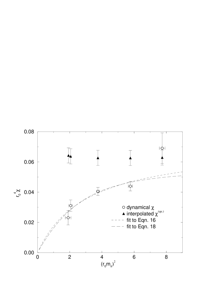
Figure 1: The measured topological susceptibility, with interpolated quenched points at the same $\hat{r}_{0}$ and fits independent of the quenched points.

In Table 1 we give our estimates of the topological susceptibility. We now convert these raw lattice values into physical units using $r_{0}$ as the physical scale. In Fig. 1 we plot the resulting values of $\hat{r}_{0}^{4}\hat{\chi}$ versus a similarly scaled pseudoscalar meson mass (calculated, of course, with valence quarks that are degenerate with those in the sea, i.e. $\kappa_{\rm valence}=\kappa_{\rm sea}$). For each point we also plot the corresponding value of the quenched topological susceptibility, calculated at the same lattice spacing using the interpolation formula Eqn. 13. It is useful to note at this point the small variation in the quenched values over the range of data points simulated. This is a consequence of the UKQCD strategy of matching $\hat{r}_{0}$. Without this, if the calculations were performed at fixed $\beta$, the lattice spacing would become increasingly coarse with increasing $m_{q}$, and the reduction in the quenched susceptibility would be much more pronounced over this range of $\kappa$. We shall return to this important point when we discuss other work in a later section.

Comparing the dynamical and quenched values, the effects of the sea quarks are clear. Whilst the $(5.29,0.1340)$ point is consistent with the quenched value, moving to smaller $m_{q}$ ($\propto m_{\pi}^{2}$) the topological susceptibility is increasingly suppressed.

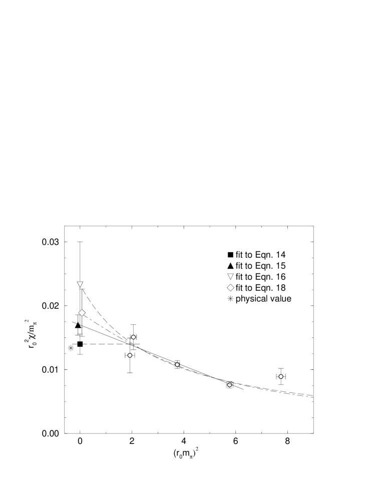
Figure 2: Fits to the measured topological susceptibility, independent of the quenched points.

We can make this observation more quantitative by attempting to fit our values of $\hat{r}_{0}^{4}\hat{\chi}$ with the expected functional form in Eqn. 7. But we must first be clear whether this fit is justified, and what exactly we are extrapolating in. Eqn. 7 is strictly a chiral expansion that describes the behaviour for small sea quark masses in the continuum and relates it to $f_{\pi}$. We expect that it is also applicable for a set of lattice data points evaluated at the same lattice spacing, except that now the decay constant, $\hat{f}_{\pi}$, will be the one appropriate to that lattice spacing. Whilst most of our data points are evaluated on a trajectory of constant lattice spacing in the parameter space, the two most chiral values are not. The lattice spacings there are slightly finer. If $\hat{r}_{0}\hat{f}_{\pi}$ varied significantly with $a$ over this range of $a$, it would not be clear how to perform a consistent chiral extrapolation through the data points. The non–perturbative improvement of the action, however, removes the leading order lattice spacing dependence and the residual corrections in this range of lattice spacings appear to be small, at least in measurements of hadron spectroscopy [16, 17]. Assuming the variation in the decay constants is similarly small over what, it should be recalled, is not a large variation in $a$, we may proceed to attempt a common chiral extrapolation to the data. For this purpose it is useful to redisplay the data in Fig. 2, where the leading order chiral behaviour would then be a horizontal line,

$$\frac{\hat{r}_{0}^{2}\hat{\chi}}{\hat{m}_{\pi}^{2}}=c_{0}\\$$ (14)

and including the leading correction gives a general straight line

$$\frac{\hat{r}_{0}^{2}\hat{\chi}}{\hat{m}_{\pi}^{2}}=c_{0}+c_{1}(\hat{r}_{0}\hat{m}_{\pi})^{2}.$$ (15)

In each case the intercept is related to the decay constant by $c_{0}=(\hat{r}_{0}\hat{f}_{\pi})^{2}/4$. We now follow a standard fitting procedure, first using the most chiral points, then systematically adding the less chiral points until the fit becomes unacceptably bad. The larger the number of points one can add in this way, the more evidence one has for the fitted form and the more confident one is that the systematic errors, associated with the neglected higher order corrections, are small. The results of performing such fits are shown in Table 2 and those using the two and four most chiral points respectively are plotted on Fig. 2. We see from the Table that the fits using Eqn. 15 show much greater stability and these are the ones that will provide our eventual best estimate for $f_{\pi}$.

We should comment briefly on the determination of the fitting parameter errors. In performing all but the flat fit we must contend with the data having (small) errors on the abscissa in addition to the ordinate. In order to estimate their affect on the fitting parameters, we first perform fits to the data assuming that the abscissa data take their central values. Identical fits are then made using the central values plus one, and then minus one standard deviation. The spread of the fit parameters obtained provides what is probably a crude over–estimate of this error (given there is some correlation between the ordinal and abscissal uncertainties) but is sufficient to show that it is minor. We show this spread as a second error, and for estimates of the decay constant we add it in quadrature to the other fit parameter error.

It is remarkable that we can obtain stable fits to most of our data using just the first correction term in Eqn. 15. Nonetheless, as we can see in Fig. 1, our values of the susceptibility are not very much smaller than the $m_{\pi}=\infty$ quenched value and we need to have some estimate of the possible systematic errors that may arise from neglecting the higher order corrections that will eventually check the rise in $\hat{\chi}$. As discussed earlier we shall do so by exploring two possibilities. One is that the reason why $\hat{\chi}$ is close to $\hat{\chi}^{\rm qu}$ is not that $m_{q}$ is ‘large’ but rather that $N_{c}=3$ is large. Then the values of $\hat{\chi}$ should follow the form in Eqn. 8. A second possibility is simply that our values of $m_{q}$ are indeed large. In that case we have argued that the functional form Eqn. 9 should be a reasonable representation of the true mass dependence. We now perform both types of fit in turn.

We begin with the first possibility, and therefore fit the data with the following ansatz

$$\hat{r_{0}}^{4}\hat{\chi}=\frac{c_{0}c_{3}(\hat{r}_{0}\hat{m}_{\pi})^{2}}{c_{3}+c_{0}(\hat{r}_{0}\hat{m}_{\pi})^{2}},$$ (16)

where we expect $c_{3}$ = $\hat{r_{0}}^{4}\hat{\chi}^{\rm qu}$ up to ${\cal O}(1/N_{c}^{2})$ corrections. To test this we fit up to six data points. The first five are measured in the dynamical simulations. The final quantity is the quenched susceptibility at a lattice spacing equivalent to those of the three least chiral, “matched” ensembles. The last is assigned an arbitary large value $(\hat{r}_{0}\hat{m}_{\pi})^{2}=1000$ whose exact value has no effect on the fits.

We also expect, from the Maclaurin chiral expansion of Eqn. 16,

$$\hat{r_{0}}^{4}\hat{\chi}=c_{0}\cdot(\hat{r}_{0}\hat{m}_{\pi})^{2}-c_{0}^{2}/c_{3}\cdot(\hat{r}_{0}\hat{m}_{\pi})^{4}+c_{0}^{3}/c_{3}^{2}\cdot(\hat{r}_{0}\hat{m}_{\pi})^{6}+{\cal O}((\hat{r}_{0}\hat{m}_{\pi})^{8})$$ (17)

that $c_{0}$ is related to the decay constant as before, $c_{0}=(\hat{r}_{0}\hat{f}_{\pi})^{2}/4$. We present the results of the fits in Table 3.

We turn now to fits based on the functional form in Eqn. 9. We therefore use the ansatz

$$\hat{r_{0}}^{4}\hat{\chi}=\frac{2c_{0}}{\pi}(\hat{r}_{0}\hat{m}_{\pi})^{2}\tan^{-1}\left(\frac{c_{3}}{\frac{2c_{0}}{\pi}(\hat{r}_{0}\hat{m}_{\pi})^{2}}\right)$$ (18)

where once again we expect $c_{3}$ = $\hat{r_{0}}^{4}\hat{\chi}^{\rm qu}$ and from the expansion

$$\hat{r_{0}}^{4}\hat{\chi}=c_{0}(\hat{r}_{0}\hat{m}_{\pi})^{2}-\left(\frac{2c_{0}}{\pi}\right)^{2}\cdot\left(\frac{1}{c_{3}}\right)\cdot(\hat{r}_{0}\hat{m}_{\pi})^{4}+{\cal O}((\hat{r}_{0}\hat{m}_{\pi})^{8})$$ (19)

we expect $c_{0}=(\hat{r}_{0}\hat{f}_{\pi})^{2}/4$. Note that in contrast to Eqn. 17, Eqn. 19 has no term that is cubic in $m_{q}$ and the rise will remain approximately quadratic for a greater range in $(\hat{r}_{0}\hat{m}_{\pi})^{2}$. That this need be no bad thing is suggested by the relatively large range over which we could fit Eqn. 15. And indeed we see from the fits listed in Table 3 that this form fits our data quite well.

Typical examples of the fits from Eqn. 16 and Eqn. 18 are shown in Figs. 1 and 2. The similarity of the two functions is apparent. In Table 4 we use the fit parameters to construct the first three expansion coefficients in the Maclaurin series for the various fit functions, describing the chiral behaviour of $\chi$. The fits are consistent with one another.

The fitted asymptote of the susceptibility at large $m_{q}$ is given by $c_{3}$. We see from Table 3 that these are broadly consistent with the quenched value, and our large statistical errors do not currently allow us to resolve any ${\cal O}(1/N_{c}^{2})$ deviation from this.

As an aside we ask what happens if we cast aside some of our theoretical expectations and ask how strong is the evidence from our data that (a) the dependence is on $m_{\pi}^{2}$ rather than on some other power, and (b) the susceptibility really does go to zero as $m_{\pi}\to 0$? To answer the first question we perform fits of the kind in Eqn. 18 but replacing $(\hat{r}_{0}\hat{m}_{\pi})^{2}$ by $(\hat{r}_{0}\hat{m}_{\pi})^{c}$. We find, using all six values of $\hat{\chi}$, that $c=1.64(22)(8)$; a value consistent with $c=2$. The $\chi^{2}$/d.o.f. is poorer, however, than for the fit with a power fixed to 2 (possible as there is one fewer d.o.f.) suggesting that the data does not warrant the use of such an extra parameter. As for the second question, we add a constant $\hat{c}$ to Eqn. 18 and find $\hat{c}=0.0096(78)(20)$. Again this is consistent with our theoretical expectation; and again the $\chi^{2}$/d.o.f. is worse. (See Table 5 for details of the above two fits.)

Given the consistency of our description of the small $m_{\pi}$ regime from our measurements it is reasonable to use the values of $c_{0}$ to estimate the pion decay constant, $f_{\pi}$. This is done in units of $r_{0}$ in Tables 2 and 3. We use the chiral fit of Eqn. 15 over the largest acceptable range to provide us with our best estimate and its statistical error. We then use the fits with other functional forms to provide us with the systematic error. This produces an estimate

$$\hat{r}_{0}\hat{f}_{\pi}=0.261\ \pm 0.013\ ^{+0.045}_{-0.025}$$ (20)

where the first error is statistical and the second is systematic. This is of course no more than our best estimate of the value of $f_{\pi}$ corresponding to our lattice spacing of $a\simeq 0.1\mathop{\rm fm}$. This value will contain corresponding lattice spacing corrections and these must be estimated before making a serious comparison with the experimental value. Our use of the non-perturbative $c_{\rm sw}$ should have eliminated the leading ${\cal O}(a)$ errors, however, and $(a/r_{0})^{2}$ is sufficiently small that it is plausible to expect these lattice corrections to be smaller than our other errors. If we use the phenomenological value $r_{0}=0.49\ \mathop{\rm fm}$ then we obtain from Eqn. 20 the value

$$f_{\pi}=105\ \pm 5\ ^{+18}_{-10}\ \mathop{\rm MeV}$$ (21)

which is reasonably close to the experimental value $\simeq 93\ \mathop{\rm MeV}$. In [3] a comparison with other physical quantities is expected to provide us with a quantitative estimate of the magnitude of the ${\cal O}(a^{2})$ errors.

4 Comparison with other studies

During the course of this work, there have appeared some other studies of the topological susceptibility in lattice QCD; in particular one by the CP-PACS collaboration [18], and one by the Pisa group [19]. Both calculations find no significant decrease of the susceptibility with decreasing quark (or pion) mass when everything is expressed in physical, rather than lattice, units. This appears to contradict our findings and is clearly something we need to address.

Our suggestion why these other studies have seen no decrease in $\chi$ is as follows. They differ from our study in having been performed at fixed $\beta$. That implies that the lattice spacing $a$ decreases as $m_{q}$ is decreased. In typical current calculations this variation in $a$ is substantial. (See for example Fig. 4 of [20].) At the smallest values of $m_{q}$ the lattice spacing cannot be allowed to be too fine, because the total spatial volume must remain adequately large. This implies that at the larger values of $m_{q}$ the lattice spacing is quite coarse. Over such a range of lattice spacings the topological susceptibility in the pure gauge theory typically shows a large variation. Since for coarser $a$ more instantons (those with $\rho\leq{\cal O}(a)$) are excluded, and more of those remaining are narrow in lattice units (with a correspondingly suppressed lattice topological charge) we expect that this variation is quite general, and not a special feature of the pure gauge theory with a Wilson action. In lattice QCD we therefore expect two simultaneous effects in $\hat{\chi}$ as we decrease $m_{q}$ at fixed $\beta$. First, because of the ${\cal O}(a^{2})$ lattice corrections just discussed, $\hat{\chi}$ will, like $\hat{\chi}^{\rm qu}$, tend to increase. Second, it will tend to decrease because of the physical quark mass dependence. In the range of quark masses covered in current calculations this latter decrease is not very large (as we have seen in our work) and we suggest that the two effects may largely compensate each other so as to produce a susceptibility that shows very little variation with $m_{q}$; in contrast to the ratio $\hat{\chi}/\hat{\chi}^{\rm qu}$ which does.

To illustrate this consider the fixed-$\beta$ calculation in [20]. The range of quark masses covered in that work corresponds to $(\hat{r}_{0}\hat{m}_{\pi})^{2}$ decreasing from about 6.5 to about 3.0. Simultaneously $a/r_{0}$ decreases from about 0.437 to about 0.274. Over this range of $1/\hat{r}_{0}\equiv a/r_{0}$ the pure gauge susceptibility increases by almost a factor of two, as we see using Eqn. 13. Clearly this is large enough to compensate for the hoped–for near–chiral variation of the susceptibility.

To make this a little more quantitative we consider the different calculations in turn, beginning with that in [19]. The Pisa group uses the Wilson gauge action, and four flavours of staggered fermions. Simulations are carried out at a fixed value of the gauge coupling for a range of bare quark masses between $\hat{m}_{q}=0.01$ and 0.05. Expressed in units of the string tension, $\sigma$, this corresponds to a change in the quark mass by a factor of approximately three. Over the corresponding range of lattice spacings the susceptibility in the pure gauge theory with Wilson action varies by a factor of $1.44(19)$, when determined using the same “field theoretic + smearing” method (for a review, see [9]). Such an increase would be large enough to largely compensate for the hoped–for near chiral decrease of the susceptibility (see for example the variation of $\hat{r}^{4}_{0}\hat{\chi}$ between $(\hat{r}_{0}\hat{m}_{\pi})^{2}\simeq 6.0$ and $\simeq 2.0$ in Fig. 1).

The CP-PACS study is carried out using an improved (Iwasaki) gauge action with two flavours of tadpole–improved Sheikoslami–Wohlert clover fermions. Combining the data from [18, 21], one finds over the range of quark masses considered a variation in the square of the pion mass (in units of the string tension) of approximately 3, similar to that of the Pisa study. Over this range there is also little variation in the topological susceptibility when expressed in units of the string tension. The string tensions considered would correspond, in a pure gauge Wilson action study, to a range in $\beta$ of $5.64-5.71$, and in that range the topological susceptibility, $\hat{\chi}^{\rm qu}$, varies by a factor of around 1.5. If we assume that there is a similar effect with the Iwasaki action, then over this range the dynamical $\hat{\chi}$ appears to suffer a suppression of about a factor of 1.5 relative to the pure gauge theory. As before, not all the data is near the chiral limit, and over a corresponding range in the UKQCD data we see a suppression of around a factor of 2. CP-PACS in fact possess datasets at four values of $\beta$ and they have calculated the topological susceptibility on the dataset corresponding to the second smallest value. At their higher values of $\beta$ the effect we have been describing here will be much weaker and we believe that calculations performed on those two datasets will reveal a quark mass dependence comparable to the one we find.

The arguments presented in this section are by no means definitive. We do not, for instance, know the discretisation effects on the topological susceptibility in lattice gluodynamics with the Iwasaki action. Neither do we know know how the (different) fermionic actions alter these discretisation effects. What the heuristic analysis given here aims to show is that these results are not necessarily in contradiction to the theoretical expectations and to the results presented in this talk.

5 Conclusions

We have calculated the topological susceptibility in lattice QCD with two light quark flavours, using lattice field configurations, recently generated by UKQCD, in which the lattice spacing is approximately constant as the quark mass is varied. We find that there is clear evidence of the effects of sea quarks in suppressing $\chi$.

We discuss this behaviour in the context of chiral and large $N_{c}$ expansions, and find good agreement with the functional forms expected there. We are not able to make a stronger statement about how close QCD is to its large $N_{c}$ limit, owing to the relatively large statistical errors on our calculated values, particularly at larger quark masses.

The consistent leading order chiral behaviour from our various fitting ansätze allows us to make an estimate for the pion decay constant, $f_{\pi}=105\ \pm 5\ ^{+18}_{-10}\ \mathop{\rm MeV}$, for the lattice spacing of $a\simeq 0.1\mathop{\rm fm}$. (Here the first error is statistical and the second has to do with the chiral extrapolation.) Since we use a lattice fermion action in which the leading ${\cal O}(a)$ discretisation errors have been removed, and (quenched) hadron masses show little residual lattice spacing dependence, we might expect that this value is close to its continuum limit. In any case we note that it is in agreement with the experimental value, $\simeq 93\ \mathop{\rm MeV}$.

We have commented on some recent studies of the topological susceptibility in lattice QCD, which do not see the kind of mass dependence that we claim to have observed. We have suggested that this might arise from the fact that in these fixed-$\beta$ calculations the value of $a$ decreases with decreasing $m_{\pi}^{2}$ and the consequent variation in those ${\cal O}(a^{2})$ lattice corrections that the susceptibility (plausibly) shares with the pure gauge theory might be large enough to compensate for the expected near–chiral variation. Further analysis of this and the corresponding quenched theories in this light would be welcome.

$(\beta,\kappa)$	$\hat{\chi}\times 10^{5}$
(5.20, 0.13565)	3.	18 (64)
(5.20, 0.13550)	4.	84 (57)
(5.20, 0.13500)	7.	90 (42)
(5.26, 0.13450)	8.	86 (54)
(5.29, 0.13400)	12.	9 (1.9)

Table 1: The topological susceptibility in lattice units.

Fit	$N_{\rm fit}$	$c_{0}$		$c_{1}$		$\chi^{2}/{\rm d.o.f.}$		$\hat{r}_{0}\hat{f}_{\pi}$
Eqn. 14	2	0.	0140 (16)	—		0.	805	0.	237 (14)
Eqn. 14	3	0.	0112 (6)	—		2.	202	0.	212 (6)
Eqn. 14	4	0.	0091 (4)	—		9.	008	—
Eqn. 15	3	0.	0176 (35) (4)	$-0$.	0018 (10) (1)	0.	964	0.	265 (27)
Eqn. 15	4	0.	0170 (16) (1)	$-0$.	0016 (4) (0)	0.	502	0.	261 (13)
Eqn. 15	5	0.	0147 (14) (1)	$-0$.	0011 (3) (0)	2.	965	0.	242 (12)

Table 2: Fits to the $N_{\rm fit}$ most chiral points of $(\hat{r}_{0}^{2}\hat{\chi})/\hat{m}_{\pi}^{2}$.

Fit	$N_{\rm fit}$	$c_{0}$		$c_{3}$		$\chi^{2}/{\rm d.o.f.}$		$\hat{r}_{0}\hat{f}_{\pi}$
Eqn. 16	3	0.	0208 (87) (12)	0.	0844 (427) (35)	1.	013	0.	288 (61)
Eqn. 16	4	0.	0272 (85) (18)	0.	0632 (114) (6)	0.	895	0.	329 (53)
Eqn. 16	5	0.	0233 (66) (10)	0.	0717 (147) (3)	1.	847	0.	305 (44)
Eqn. 16	6	0.	0279 (32) (11)	0.	0631 (5) (0)	1.	489	0.	334 (21)
Eqn. 18	3	0.	0186 (53) (7)	0.	0576 (175) (6)	0.	990	0.	273 (40)
Eqn. 18	4	0.	0209 (42) (7)	0.	0506 (55) (5)	0.	682	0.	289 (30)
Eqn. 18	5	0.	0189 (36) (5)	0.	0550 (69) (6)	1.	929	0.	275 (27)
Eqn. 18	6	0.	0164 (14) (7)	0.	0629 (5) (0)	1.	567	0.	256 (12)

Table 3: Fits to the $N_{\rm fit}$ most chiral points of $(\hat{r}_{0}^{4}\hat{\chi})$.

Fit	$N_{\rm fit}$	const.		${\cal O}((\hat{r}_{0}\hat{m}_{\pi})^{2})$		${\cal O}((\hat{r}_{0}\hat{m}_{\pi})^{4})$
Eqn. 15	4	0.	0170 (17)	$-0$.	0016 (4)	—
Eqn. 16	5	0.	0233 (67)	$-0$.	0031 (19)	0.	0025 (24)
Eqn. 16	6	0.	0279 (34)	$-0$.	0123 (30)	0.	0055 (19)
Eqn. 18	5	0.	0189 (37)	$-0$.	0026 (11)	0
Eqn. 18	6	0.	0164 (16)	$-0$.	0017 (4)	0

Table 4: Chiral expansion terms of fitted functions.

$N_{\rm fit}$	$c_{0}$		$c_{3}$		$c$		$\hat{c}$		$\chi^{2}/{\rm d.o.f.}$
6	0.	0112 (40) (5)	0.	0533 (78) (17)	fixed to 2		0.	0096 (78) (20)	1.	825
6	0.	0206 (26) (16)	0.	0631 (80) (49)	1.	64 (22) (8)	fixed to 0		1.	798

Table 5: Fits to the $N_{\rm fit}$ most chiral values of $(\hat{r}_{0}^{4}\hat{\chi})$; for the power $c$ of $m^{2}_{\pi}$, and for the chiral intercept, $\hat{c}$. These are as described in the text.

References

- [1] M. Teper, hep-lat/9909124.
- [2] A. Hart, M. Teper, hep-lat/9909072.
- [3] UKQCD collaboration, in preparation.
- [4] P. Di Vecchia, G. Veneziano, Nucl. Phys. B 171 (1980) 253.
- [5] H. Leutwyler, A. Smilga, Phys. Rev. D 46 (1992) 5607.
- [6] G. ‘t Hooft, Nucl. Phys. B72 (1974) 461.
- [7] E. Witten, Nucl. Phys. B160 (1979) 57.
- [8] M. Teper, Phys. Rev. D 59 (1999) 014512 [hep-lat/9804008].
- [9] M. Teper, hep-th/9812187.
- [10] J. Garden (UKQCD), hep-lat/9909066.
- [11] A. Irving et al., Phys. Rev. D 58 (1998) 114504 [hep-lat/9807015].
- [12] R. Sommer, Nucl. Phys. B411 (1994) 839 [hep-lat/9310022].
- [13] D. Smith, M. Teper, Phys. Rev. D 58 (1998) 014505 [hep-lat/9801008].
- [14] P. di Vecchia et al., Nucl. Phys. B192 (1981) 392.
- [15] M. Campostrini, A. Di Giacomo, H. Panagopoulos, Phys. Lett. B212 (1988) 206.
- [16] H. Wittig, Nucl. Phys. (Proc.Suppl.) 63 (1998) 47 [hep-lat/9710013].
- [17] R. Edwards, U. Heller, T. Klassen, Phys. Rev. Lett. 80 (1998) 3448 [hep-lat/9711052].
- [18] A. Ali Khan et al. (CP-PACS), hep-lat/9909045.
- [19] B. Allés, M. D’Elia, A. Di Giacomo, hep-lat/9912012.
- [20] C. Allton et al. (UKQCD), Phys.Rev. D60 (1999) 034507, [hep-lat/9808016].
- [21] A. Ali Khan et al. (CP-PACS), hep-lat/9909050; S. Aoki et al. (CP-PACS), hep-lat/9809120; R. Burkhalter, private communication.