[

Neutrinos and Gauge Unification

Abstract

The approximate unification of gauge couplings is the best indirect evidence for low-energy supersymmetry, although it is not perfect in its simplest realizations. Given the experimental evidence for small non-zero neutrino masses, it is plausible to extend the MSSM with three right-handed neutrino chiral multiplets, with large Majorana masses below the unification scale, so that a see-saw mechanism can be implemented. In this extended MSSM, the unification prediction for the strong gauge coupling constant at $M_{Z}$ can be lowered by up to $\sim 5\%$, bringing it closer to the experimental value at $1\sigma$, therefore improving significantly the accuracy of gauge coupling unification.

]

Gauge coupling unification is an important test for candidates to fundamental theories beyond the Standard Model (SM). On the one hand, gauge unification is a prediction of most of such theories. In particular, GUT models predict the unification of the gauge couplings at a scale $\sim M_{X}$, corresponding to the breakdown of the unifying group. Also, most of the string constructions predict unification of all the gauge couplings, including gravity, even in the absence of a GUT group. On the other hand, due to the present high-precision knowledge of the gauge couplings at low energy, one can extrapolate them to high energy through the corresponding renormalization group equations (RGEs) and verify whether unification takes place or not.

Of course the evolution of the couplings (as described by the RGEs) depends on the type of theory under study. In particular, unification can depend on whether it is supersymmetric or not, whether it has the minimal matter content or not, whether it has (large) extra dimensions or not, etc. Consequently, the requirement of gauge coupling unification offers the possibility of testing these theories at very high scales. In this respect, it has been known for a long time that non-supersymmetric gauge unification (with minimal matter content) does not work. In contrast, supersymmetric gauge unification takes place with remarkable accuracy at $M_{X}\sim 2\times 10^{16}$ GeV. This fact was confirmed in 1990 with the precise LEP determinations of the gauge couplings. The unification occurs in such a beautiful way that it is hard to believe that it is a mere coincidence, and it is currently considered as a strong hint in favor of supersymmetry. However, there are some problems with the current status of this issue. First, the conventional prediction of (weakly coupled heterotic) superstrings is that the gauge couplings (including gravity) are unified at the string scale $M_{string}\sim 5\times 10^{17}$ GeV, which is one order of magnitude too high compared with $M_{X}$. During the last years many new string (or string-inspired) scenarios have appeared addressing this problem: strongly coupled strings, large extra dimensions, etc. Another problem is that the ordinary supersymmetric unification, however beautiful, is not perfect in the simplest scenarios. A convenient way to express the discrepancy is to start with the $SU(2)\times U(1)_{Y}$ low-energy couplings $\alpha_{1}(M_{Z})$ and $\alpha_{2}(M_{Z})$ to obtain both the unification scale and gauge coupling, $M_{X}$ and $\alpha(M_{X})$. Then, running from $M_{X}$ back to $M_{Z}$, one gets a prediction for $\alpha_{3}(M_{Z})$, to be compared to the experimental value.

Suppose then that, following for example ref. [1] one has a MSSM spectrum as obtained from a minimal supergravity model. Starting with the experimental input (in the $\overline{\rm MS}$ renormalization scheme, before conversion to the $\overline{\rm DR}$ scheme)

$$\widehat{\alpha}_{1}^{-1}(M_{Z}) = 58.98\pm 0.04,$$ (1)

$$\widehat{\alpha}_{2}^{-1}(M_{Z}) = 29.57\pm 0.03,$$ (2)

$$M_{Z} = 91.197\pm 0.007,$$ (3)

one integrates numerically two-loop RGEs, including also the supersymmetric thresholds until one finally obtains [1] a prediction $\alpha_{3}(M_{Z})\simeq 0.13$, to be compared to the experimental value [2]

$$\widehat{\alpha}_{3}(M_{Z})=0.119\pm 0.004\ ,$$ (4)

which represents a $3\sigma$ discrepancy [other evaluations give a smaller experimental uncertainty in (4), thus leading to a stronger discrepancy. We choose to be rather conservative at this point]. Several comments are in order here. The effect of supersymmetric thresholds introduces a dependence on the type of MSSM spectrum considered. For instance, the larger the supersymmetric masses, the lower $\alpha_{3}(M_{Z})$. Allowing the squark masses to be up to 1 TeV, one gets $\alpha_{3}(M_{Z})\stackrel{{\scriptstyle>}}{{{}_{\sim}}}0.127$. On the other hand, working in the context of gauge-mediated SUSY breaking, which implies the presence of extra (messenger) fields and thus a departure from the minimal matter content, one can get slightly lower values, $\alpha_{3}(M_{Z})\stackrel{{\scriptstyle>}}{{{}_{\sim}}}0.125$. This alleviates the disagreement, but it does not solve it. One would need a negative correction between$-3\%$ and $-9\%$ in $\alpha_{3}(M_{Z})$ [or a correction three times smaller in $\alpha_{3}(M_{X})$] in order to reconcile prediction and experiment. It has been argued that the origin of the discrepancy could be high-energy threshold corrections. These may be of stringy or GUT origin and are model-dependent. E.g. in a GUT scenario these corrections are due to the appearance at the GUT scale of incomplete $SU(5)$ multiplets, most notably the color triplet Higgs bosons. Demanding a threshold correction of the correct magnitude and sign severely restricts the models, e.g. minimal $SU(5)$ is incompatible with such a requirement [1].

In the present paper we explore the impact of massive neutrinos in the unification of gauge couplings. Observations of the flux of atmospheric neutrinos by SuperKamiokande [3] provide strong evidence for neutrino oscillations, which in turn imply that (at least two species of) neutrinos must be massive. Preliminary results from the long-baseline experiment K2K tend to confirm this evidence [4]. Additional support to non-zero neutrino masses is given by the need of neutrino oscillations to explain the solar neutrino flux deficit [5]. The simplest and most beautiful mechanism to account for small neutrino masses in a natural way is probably the see-saw mechanism [6]. Its supersymmetric version has superpotential

$$W=W_{MSSM}-\frac{1}{2}\nu_{R}^{c}{\cal M}\nu_{R}^{c}+\nu_{R}^{c}{\bf Y_{\nu}}L\cdot H_{2},$$ (5)

where $W_{MSSM}$ is the superpotential of the MSSM. The extra terms involve, beside the usual three lepton doublets, $L$, three additional neutrino chiral fields $\nu_{R}$ singlets under the SM group (generation indices are suppressed). ${\bf Y_{\nu}}$ is the matrix of neutrino Yukawa couplings and $H_{2}$ is the hypercharge $+1/2$ Higgs doublet. The Dirac mass matrix is ${\bf m_{D}}={\bf Y_{\nu}}v\sin\beta$. Finally, ${\cal M}$ is a $3\times 3$ Majorana mass matrix which does not break the SM gauge symmetry. It is natural to assume that the overall scale of ${\cal M}$, which we will denote by $M$, is much larger than the electroweak scale or any soft mass. Below $M$ the heavy neutrino fields can be integrated out, giving rise to an effective mass term for the left-handed neutrinos, $-\frac{1}{2}\nu^{T}{\cal M}_{\nu}\nu$, with ${\cal M}_{\nu}={\bf m_{D}}^{T}{\cal M}^{-1}{\bf m_{D}}$, suppressed with respect to the typical fermion masses by the inverse power of the large scale $M$. In fact, large values of the neutrino Yukawa couplings are perfectly consistent with tiny neutrino masses for values of $M$ sufficiently close to $M_{X}$.

The influence of heavy right-handed neutrinos on the unification of gauge couplings is due to the fact that above $M$, the Yukawa couplings ${\bf Y_{\nu}}$ of eq.(5) affect the RGEs of the gauge couplings at two-loop order, in a similar way as the top-Yukawa coupling does in the MSSM. Since ${\bf Y_{\nu}}$ can be sizeable, one expects a non-trivial impact in gauge unification. The (two-loop) RGEs at scales $Q$ between $M$ and $M_{X}$, for $g_{i}$, ${\bf Y_{t}}$ and ${\bf Y_{\nu}}$ read [with $g_{1}$ normalized as in $SU(5)$]

$$\frac{dg_{i}^{-2}}{dt} = -2\kappa\left[b_{i}+\kappa\left(b_{ij}g_{j}^{2}-a_{i\alpha}{\rm tr}{\bf H}_{\alpha}\right)\right]$$ (6)

$$\frac{d{\bf Y_{t}}}{dt} = \kappa{\bf Y_{t}}\left(-c_{i}g_{i}^{2}+3{\bf H_{t}}+{\rm T}\right)$$ (7)

$$+ \kappa^{2}{\bf Y_{t}}\left[\left(c_{i}b_{i}+\frac{c_{i}^{2}}{2}\right)g_{i}^{4}+\frac{136}{45}g_{1}^{2}g_{3}^{2}+8g_{2}^{2}g_{3}^{2}\right.$$ (8)

$$+ g_{1}^{2}g_{2}^{2}+\left(\frac{2}{5}g_{1}^{2}+6g_{2}^{2}\right){\bf H_{t}}+\left(\frac{4}{5}g_{1}^{2}+16g_{3}^{2}\right){\rm Tr}{\bf H_{t}}$$ (9)

$$- \left.9{\rm Tr}{\bf H_{t}^{2}}-4{\bf H_{t}}^{2}-3{\bf H_{t}}{\rm T}-9{\rm Tr}{\bf H^{2}_{t}}\frac{}{}\right]$$ (10)

$$\frac{d{\bf Y_{\nu}}}{dt} = \kappa{\bf Y_{\nu}}\left(-c^{\prime}_{i}g_{i}^{2}+3{\bf H}_{\nu}+{\rm T}\right)$$ (11)

$$+ \kappa^{2}{\bf Y_{\nu}}\left[\left(c_{i}^{\prime}b_{i}+\frac{c_{i}^{\prime}{}^{2}}{2}\right)g_{i}^{4}+\frac{9}{5}g_{1}^{2}g_{2}^{2}\right.$$ (12)

$$+ 6\left(\frac{1}{5}g_{1}^{2}+g_{2}^{2}\right){\bf H}_{\nu}+\left(\frac{4}{5}g_{1}^{2}+16g_{3}^{2}\right){\rm Tr}{\bf H_{t}}$$ (13)

$$- \left.3{\rm Tr}{\bf H}_{\nu}^{2}-4{\bf H}_{\nu}^{2}-3{\bf H}_{\nu}{\rm T}-9{\rm Tr}{\bf H^{2}_{t}}\frac{}{}\right]$$ (14)

(summation over repeated indices is understood) with $t=\ln Q$, $\kappa=1/(16\pi^{2})$ and

$${\bf H}_{\alpha}\equiv{\bf Y}_{\alpha}^{\dagger}{\bf Y}_{\alpha},\qquad{\rm T}\equiv{\rm Tr}(3{\bf H_{t}}+{\bf H}_{\nu}),$$ (15)

with $\alpha={\bf t},\nu$. Here ${\bf Y_{t}}$ represents the Yukawa matrix of the $u$-type quarks (dominated by the top Yukawa coupling) and the numerical coefficients are given by

$$b_{i} = (33/5,1,-3),\ \ c_{i}=(13/15,3,16/3),$$ (16)

$$c_{i}^{\prime} = (3/5,3,0),\qquad\ a_{i\alpha}=\left(\begin{array}[]{cc}26/5&6/5\\ 6&2\\ 4&0\end{array}\right),$$ (20)

$$b_{ij} = \left(\begin{array}[]{ccc}199/25&27/5&88/5\\ 9/5&25&24\\ 11/5&9&14\end{array}\right).$$ (24)

It is clear from eq.(6) that the presence of neutrinos will only affect the RGEs of $g_{1}$ and $g_{2}$. The magnitude of the final correction will depend on the numerical values of ${\bf Y_{\nu}}$ and $M$. These are not independent quantities, since the final neutrino masses ${\cal M}_{\nu}=v^{2}\sin^{2}\beta{\bf Y_{\nu}}^{T}{\cal M}^{-1}{\bf Y_{\nu}}$ (appropriately ran down to the electroweak scale [8]) must be consistent with observations. Atmospheric neutrino data only allow to determine one neutrino mass splitting, $\Delta m^{2}_{\nu}\ \sim\ 10^{-3}\ {\rm eV}^{2}$. On the other hand, ’standard’ explanations of solar neutrino flux deficits require neutrino oscillations with a much smaller mass splitting, corresponding to a different pair of neutrinos. In addition, there are upper bounds on neutrino masses, coming e.g. from the non-observation of neutrinoless double $\beta$-decay and other experiments. All this information implies that there are three possible types of neutrino spectrum: Hierarchical, $m_{1}^{2}<m_{2}^{2}\ll m_{3}^{2}$; Intermediate, $m_{1}^{2}\sim m_{2}^{2}\gg m_{3}^{2}$; and Degenerate, $m_{1}^{2}\sim m_{2}^{2}\sim m_{3}^{2}$. In the hierarchical case, the larger neutrino mass should be ${\cal O}(10^{-1}-10^{-2})\ {\rm eV}$, while in the degenerate case cosmological observations require $m_{\nu}\stackrel{{\scriptstyle<}}{{{}_{\sim}}}{\cal O}(2)\ {\rm eV}$. This means, that once a particular scenario for the neutrino spectrum is chosen, ${\bf Y_{\nu}}$ and $M$ are not independent quantities any more.

The presence of right-handed neutrinos above $M$ induces a small change both on the scale of unification and the value of the unified gauge coupling. This in turn affects the prediction of $\alpha_{3}(M_{Z})$ derived from the assumption of perfect unification. Given that the changes with respect to the MSSM case can be treated as a small perturbation, it is simple to make an analytical estimate from eqs.(6) and (14) to get:

$$\frac{\Delta\alpha_{3}(M_{Z})}{\alpha_{3}(M_{Z})^{2}}\simeq-\frac{9}{7\pi}\frac{1}{16\pi^{2}}<{\rm Tr}{\bf Y_{\nu}^{\dagger}Y_{\nu}}>\ln\frac{M_{X}}{M}.$$ (25)

In this result, $<{\rm Tr}{\bf Y_{\nu}^{\dagger}Y_{\nu}}>$ is an average value in the interval from $M$ to $M_{X}$:

$$<{\rm Tr}{\bf Y_{\nu}^{\dagger}Y_{\nu}}>\ln\frac{M_{X}}{M}=\int_{Q=M}^{M_{X}}{\rm Tr}{\bf Y_{\nu}^{\dagger}Y_{\nu}}\ d\ln Q.$$ (26)

Two important implications of Eq. (25) are, first, that neutrino corrections always make the predicted $\alpha_{3}(M_{Z})$ smaller, as required to improve the agreement with the experimental value, and second, that the effect will be important if the neutrino Yukawa couplings ${\bf Y_{\nu}}$ are sizable, which is a natural assumption, as we saw.

We can now estimate the average in Eq. (26) considering that the evolution of ${\bf Y_{\nu}}(t)$ is well described by its 1-loop RGE neglecting all couplings different from ${\bf Y_{\nu}}$. This approximation is justified if ${\bf Y_{\nu}}$ is large (the case of interest). The final result will depend on how many neutrino Yukawa couplings (or more precisely, eigenvalues of ${\bf Y_{\nu}}^{\dagger}{\bf Y_{\nu}}$) are large. With only one large neutrino coupling (this corresponds naturally to a hierarchical neutrino spectrum) it is straightforward to evaluate the integral in (26) in the approximation just described to get

$$\Delta\alpha_{3}(M_{Z})\simeq-\frac{3N}{28\pi}\alpha_{3}(M_{Z})^{2}\log\left[\frac{Y_{\nu}(M_{X})^{2}}{Y_{\nu}(M)^{2}}\right],$$ (27)

with $N=1$ counting the number of large neutrino Yukawa couplings. Of course the effect on $\alpha_{3}(M_{Z})$ is larger if all three neutrino Yukawa couplings are large (this corresponds naturally to a degenerate neutrino spectrum, but not necessarily: a hierarchy in the spectrum can be induced also in this case by flavor-dependent Majorana masses). In this $N=3$ case, the result for $\Delta\alpha_{3}(M_{Z})$ slightly depends on the kind of texture for ${\bf Y_{\nu}}$. A good estimate is given by simply taking ${\bf Y_{\nu}}=Y_{\nu}{\bf 1}$ and in that case, Eq. (27) also holds, simply setting $N=3$.

The magnitude of the correction (27) depends on the values of $Y_{\nu}$ at $M_{X}$ and $M$, but the latter is fixed in order to fit the physical neutrino mass, as explained above. Hence, the correction is just a function of a unique parameter, $Y_{\nu}(M_{X})$. [It is also a function of the neutrino mass, $m_{\nu}$, but changes on $m_{\nu}$ just imply a corresponding modification of $M$ and since the evolution of $Y_{\nu}$ occurs mainly near $M_{X}$ the final correction on $\alpha_{3}(M_{Z})$, given by eq.(27), is quite insensitive to $m_{\nu}$.] The most favorable case occurs when $Y_{\nu}(M_{X})$ is large, near a Landau pole. A representative case is $Y_{\nu}(M_{X})\sim 8$. Then $Y_{\nu}(M)\sim 2$ and we get $\Delta\alpha_{3}(M_{Z})\sim-1.4\%$ for the case $N=1$ and $\Delta\alpha_{3}(M_{Z})\sim-4.1\%$ for $N=3$. It is clear that in the first case this correction is not sufficient to reconcile $\alpha_{3}(M_{Z})$ with the experimental value, but it can be enough in the second case. These estimates agree well with our full numerical results, obtained by numerical integration of the RGEs (6-10). Now the two-loop contributions soften the RGE for ${\bf Y_{\nu}}$, which implies that ${\bf Y_{\nu}}$ decreases more slowly when the energy scale goes down. This increases the Yukawa coupling average in eq.(25), and thus the (negative) shift of the low-energy strong coupling, $\Delta\alpha_{3}(M_{Z})$.

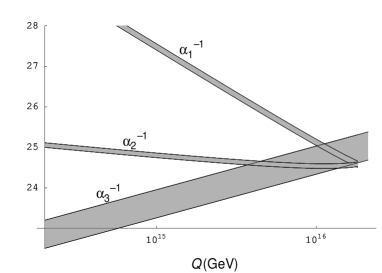
FIG. 1.: Unification of the gauge couplings $\alpha_{i}^{-1}$ for a typical MSSM scenario, without massive neutrinos (upper plot) and with them (lower plot).

An important question at this point is how large can $Y_{\nu}(M_{X})$ be without jeopardizing the perturbative expansion, and hence the reliability of the results. This has been studied in great detail in ref.[10] for the case of the top Yukawa coupling. Since, in the large coupling regime relevant for this question, the RGEs for the top and neutrino Yukawa couplings (in the $N=3$ case) are identical, the results of ref. [10] are applicable also to the present case. The conclusions of the authors of ref. [10], using Padé-Borel resummations of the 4-loop beta-function, were that the qualitative behaviour of the running is well described by the one-loop approximation and can be further improved by Padé-Borel approximants which are reliable for values of the Yukawa coupling up to $\stackrel{{\scriptstyle<}}{{{}_{\sim}}}8$ (For the $N=1$ case this is a conservative estimate, since in that case the beta-function for $Y_{\nu}$ is softer than that of $Y_{t}$.). We have used a $[1,1]$ Padé-Borel resummation of the ${\bf Y_{\nu}}$ beta-function to obtain our most reliable numerical results. As the beta-function in this approximation is smaller than at one-loop, the final result for the average in (25) turns out to be a bit larger than our analytical estimates [for a fixed value of $Y_{\nu}(M_{X})$]. The negative shift on $\alpha_{3}(M_{Z})$ goes then from 4% to about 5%. This fact, together with the uncertainties in $\alpha_{1}(M_{Z})$, $\alpha_{2}(M_{Z})$ and the top mass, imply that the usual MSSM scenarios, which yielded an unsuccessful prediction $\alpha_{3}(M_{Z})\simeq 0.13$, are now rescued within $1\sigma$ confidence level. [The agreement can be perfect in other MSSM scenarios, which predict slightly lower values of $\alpha_{3}(M_{Z})$, even if the error in (4) becomes smaller.]

This is illustrated in fig. 1 for a typical MSSM scenario The first plot shows how the gauge couplings fail to unify in the ordinary MSSM in the absence of massive neutrinos (the requirement of unification would imply $\alpha_{3}(M_{Z})=0.13$ in the case plotted). The second plot corresponds to the MSSM extended with neutrinos getting mass via a see-saw mechanism. More precisely, the plot corresponds to a scenario with degenerate neutrinos of mass $m_{\nu}=2$ eV and $Y_{\nu}(M_{X})=8$. It is apparent how the $\alpha_{1}$ and $\alpha_{2}$ runnings are modified in a suitable way to get gauge unification.

Besides the logarithmic effect on unification we have described, the presence of heavy right-handed neutrinos affects the running of the gauge couplings also through finite two-loop threshold effects at the Majorana scale $M$. However, these will depend on the neutrino Yukawa coupling $Y_{\nu}(M)$, which in the case of interest is much smaller than $Y_{\nu}(M_{X})$, so that it is safe to neglect these matching effects.

Finally, it is interesting to point out that effects similar to the ones we have found are expected in the next-to-minimal supersymmetric standard model (NMSSM), i.e. the MSSM extended with a singlet chiral multiplet $S$. The superpotential of the NMSSM does not contain a mass term for the Higgs multiplets (the $\mu$-term). However, an effective $\mu$ term of the correct order of magnitude is generated dynamically by $\Delta W=Y_{s}SH_{1}\cdot H_{2}$, when $S$ takes a vacuum expectation value. This solves in fact the $\mu$ problem of the MSSM and is one of the main virtues of the NMSSM (although this model has its own drawbacks). The influence of the new Yukawa coupling $Y_{s}$ on the running of the gauge couplings is also a two-loop effect, of exactly the same form as in (6) with $Y_{s}^{2}$ instead of ${\rm Tr}{\bf H_{\nu}}$ (the coefficients $a_{\alpha i}$ are exactly the same for $\alpha=\nu$ and $\alpha=s$). The final impact on $\alpha_{3}(M_{Z})$ is therefore given by a formula like (25) with ${\rm Tr}{\bf Y_{\nu}^{\dagger}Y_{\nu}}$$\rightarrow$$Y_{s}^{2}$ and $M$ replaced by the mass $M_{S}$ of the singlet $S$, which is close to the electroweak scale (this makes the logarithm much larger). Numerically, we find $\Delta\alpha_{3}(M_{Z})\simeq-3\%$ for $M_{S}=1$ TeV and $Y_{s}(M_{X})=8$. Similar effects can occur in other extensions of the MSSM with additional Yukawa couplings, as has been shown for models with $R$-parity violating couplings in ref. [9].

In conclusion, we have examined the impact of heavy see-saw neutrinos (plausible in view of the growing experimental evidence in favor of non-zero neutrino masses) on the unification of gauge couplings, in particular as reflected in the unification prediction for the strong gauge coupling constant at the electroweak scale. We find that the effect is small, but is always of the right sign and can be of the right magnitude to bring the too high MSSM prediction for $\alpha_{3}(M_{Z})$ down to values within $1\sigma$ of the experimental value. Given that adding three heavy right-handed neutrinos is not an ad-hoc extension of the MSSM but on the contrary is well motivated by experiment and theory alike, this result is welcome and noticeable. This effect should be taken into account, even in models with sizeable stringy or GUT high-energy threshold corrections. For example, models that have been discarded for not giving the appropriate threshold corrections (e.g. minimal $SU(5)$, [1]), can be now perfectly consistent.

Acknowledgments We thank H. Dreiner for useful correspondence. We also thank A. Delgado for very useful discussions. A. I. thanks the Comunidad de Madrid (Spain) for a pre-doctoral grant.

REFERENCES

- [1] J. Bagger, K. Matchev and D. Pierce, Phys. Lett. B348 (1995) 443 ; P. Langacker and N. Polonsky, Phys. Rev. D52 (1995) 3081 .
- [2] C. Caso et al., Eur. Phys. J. C3 (1998) 1.
- [3] Y. Fukuda et al. [Super-Kamiokande], Phys. Lett. B433 (1998) 9 ; Phys. Lett. B436 (1998) 33 ; Phys. Rev. Lett. 81 (1998) 1562 ; Phys. Rev. Lett. 82 (1999) 2644 .
- [4] Y. Oyama, [K2K], hep-ex/0004015
- [5] W. Hampel et al. [GALLEX], Phys. Lett. B388 (1996) 384; D. N. Abdurashitov et al. [SAGE], Phys. Rev. Lett. 77 (1996) 4708; Y. Fukuda et al. [Kamiokande], Phys. Rev. Lett. 77 (1996) 1683; Y. Fukuda et al. [Super-Kamiokande], Phys. Rev. Lett. 82 (1999) 2430 ; Phys. Rev. Lett. 82 (1999) 1810 .
- [6] M. Gell-Mann, P. Ramond and R. Slansky, proceedings of the Supergravity Stony Brook Workshop, New York, 1979, eds. P. Van Nieuwenhuizen and D. Freedman (North-Holland, Amsterdam); T. Yanagida, proceedings of the Workshop on Unified Theories and Baryon Number in the Universe, Tsukuba, Japan 1979 (edited by A. Sawada and A. Sugamoto, KEK Report No. 79-18, Tsukuba); R. Mohapatra and G. Senjanović, Phys. Rev. Lett. 44 80 912, Phys. Rev. D23 81 165.
- [7] D. R. Jones, Nucl. Phys. B87 (1975) 127; P. West, Phys. Lett. B137 (1984) 371; D. R. Jones and L. Mezincescu, Phys. Lett. B136 (1984) 242; Phys. Lett. B138 (1984) 293; M. E. Machacek and M. T. Vaughn, Nucl. Phys. B236 (1984) 221; Nucl. Phys. B249 (1985) 70; S. P. Martin and M. T. Vaughn, Phys. Rev. D50 (1994) 2282 .
- [8] P. H. Chankowski and Z. Pluciennik, Phys. Lett. B316 (1993) 312 ; K. S. Babu, C. N. Leung and J. Pantaleone, Phys. Lett. B319 (1993) 191 .
- [9] B. C. Allanach, A. Dedes and H. K. Dreiner, Phys. Rev. D60 (1999) 056002 .
- [10] P. M. Ferreira, I. Jack and D. R. Jones, Phys. Lett. B392 (1997) 376 .