RELAXING NEAR THE CRITICAL POINT

Abstract

Critical slowing down of the relaxation of the order parameter has phenomenological consequences in early universe cosmology and in ultrarelativistic heavy ion collisions. We study the relaxation rate of long-wavelength fluctuations of the order parameter in an $O(N)$ scalar theory near the critical point to model the non-equilibrium dynamics of critical fluctuations near the chiral phase transition. A lowest order perturbative calculation (two loops in the coupling $\lambda$) reveals the breakdown of perturbation theory for long-wavelength fluctuations in the critical region and the emergence of a hierarchy of scales with hard $q\geq T$, semisoft $T\gg q\gg\lambda T$ and soft $\lambda T\gg q$ loop momenta which are widely separated in the weak coupling limit. A non-perturbative resummation is implemented to leading order in the large $N$ limit which reveals the infrared renormalization of the static scattering amplitude and the crossover to an effective three dimensional theory for the soft loop momenta near the critical point. The effective three dimensional coupling is driven to the Wilson-Fisher three dimensional fixed point in the soft limit. This resummation provides an infrared screening and for critical fluctuations of the order parameter with wave-vectors $\lambda T\gg k\gg k_{us}$ or near the critical temperature $\lambda T\gg m_{T}\gg k_{us}$ with the ultrasoft scale $k_{us}=\frac{\lambda T}{4\pi}\exp{[-\frac{4\pi}{\lambda}]}$ the relaxation rate is dominated by classical semisoft loop momentum leading to $\Gamma(k,T)=\lambda T/(2\pi N)$. For wavectors $k\ll k_{us}$ the damping rate is dominated by hard loop momenta and given by $\Gamma(k,T)=4\pi T/\left[3N\ln(T/k)\right]$. Analogously, for homogeneous fluctuations in the ultracritical region $m_{T}\ll k_{us}$ the damping rate is given by $\Gamma_{0}(m_{T},T)=4\pi T/\left[3N\ln(T/m_{T})\right]$. Thus critical slowing down emerges for ultrasoft fluctuations. In such regime the rate is independent of the coupling $\lambda$ and both perturbation theory and the classical approximation within the large $N$ limit break down. The strong coupling regime and the shortcomings of the quasiparticle interpretation are discussed.

I Introduction and Motivation

The program of relativistic heavy ion collisions both at Brookhaven and at Cern seeks to understand the phase diagram of QCD in conditions of temperatures that were achieved during the first 10$\mu$s after the Big Bang or densities several times that of nuclear matter which could exist at the center of neutron stars. Current theoretical understanding[1] leads to the conclusion that QCD could undergo two phase transitions: a confinement-deconfinement (or hadronization) and the chiral phase transition. Current lattice data seem to suggest that both occur at about the same temperature $T_{c}\approx 160\mbox{MeV}$[1]. The consensus emerging in the field is that several types of observables will have to be studied simultaneously and event-by-event analysis of data will have to be carried out to extract unambiguous signals both hadronic and electromagnetic to reveal the presence of a Quark-Gluon Plasma phase. Recent results reported from CERN-SPS[2] seem to indicate a strong evidence for the existence of the QGP in Pb-Pb collisions, and RHIC at Brookhaven will begin operation soon with Au-Au collisions with four dedicated detectors capable of event-by-event analysis of hadronic and electromagnetic observables.

For QCD with only two flavors of massless quarks (u,d) it has been argued[3, 4] that the chiral phase transition at finite temperature but vanishing baryon number density is of second order and described by the universality class of O(4) Heisenberg ferromagnets. It has also been suggested recently that at finite baryon density there is a second order critical point described by the Ising universality class[5]. Second order critical points are characterized by strong critical long-wavelength fluctuations and a diverging correlation length that could lead to important experimental signatures[6]. These signatures would be akin to critical opalescence near the critical point in binary fluids[6] and could be observed in an event-by-event analysis of the fluctuations of the charged particle transverse momentum distribution (mainly pions)[6]. These fluctuations are characterized by the typical correlation length of the order parameter and it has been suggested that the phenomenon of critical slowing down, ubiquitous near the critical point of second order phase transitions, can lead to strong departures from equilibrium that will determine the value of the correlation length when long-wavelength fluctuations freeze out[7]. Critical slowing down of long-wavelength fluctuations near a second order critical point is the statement that the long-wavelength Fourier components of the order parameter relax very slowly towards equilibrium[8]. In mean-field theory in classical critical phenomena, the relaxation time diverges proportional to the susceptibility near the critical temperature but thermal fluctuations renormalize the relaxation time to be of the form $\tau(\vec{k}=0)\propto\xi^{z}$ with $\xi$ the correlation length, or at critical point $\tau(k)\propto k^{z}$ with $z$ a dynamical critical exponent [8, 9]. Another similar manifestation of an anomalously slow relaxation of long-wavelength fluctuations arises in weakly first order phase transitions when the system enters into the mixed phase where the (isothermal) speed of sound, which determines the velocity of propagation of long-wavelength pressure waves, becomes anomalously small resulting in the softest point of the equation of state. In this case there have also been suggestions that there are experimental consequences of this softening in relativistic heavy ion collisions in observables related to collective flow and the transverse momentum distributions of particles at freezeout[10].

In classical normal fluids near the critical point the vanishing of the (isothermal) speed of sound, critical opalescence (strong scattering of light by long-wavelength fluctuations) and critical slowing down are all related[11], and in ferromagnets the spin diffusion constant vanishes near the critical point again signaling critical slowing down[11].

The softening of the equation of state near the critical point of QCD could also have important cosmological implications. When the the QGP enters the mixed phase with hadrons, the speed of sound becomes anomalously small and the time scale for propagation of pressure waves over a given critical wavelength becomes longer than the free fall time for gravitational collapse which is then unhindered by the pressure of the hadronic gas. This could lead to the formation of primordial black holes[12] with a possible imprint in the acoustic peaks in the cosmic microwave background[13]. Other possible cosmological relics from the QCD phase transition with a mixed phase had been predicted, from strange quark nuggets to MACHO’s[14, 15].

A familiar argument is typically invoked to state that while the QCD phase transition in the Early Universe occurred in local thermodynamic equilibrium (LTE) this may not be the case in Relativistic Heavy Ion Collisions. The argument compares the typical collisional relaxation time scale obtained from a strong interaction process $\tau_{coll}\sim 10^{-22}~{}\mbox{secs}$ to the time scale for cooling near the critical temperature $\sim 160\mbox{MeV}$, i.e. ${T/\dot{T}}\sim H^{-1}\sim 10^{-5}~{}\mbox{secs}$. The argument is that since $\tau_{coll}\ll H^{-1}$ the phase transition occurs in LTE in cosmology, whereas in relativistic heavy ion collisions at RHIC and LHC energies these time scales will be comparable. However this argument completely neglects the possibility that long-wavelength fluctuations could undergo critical slowing down and freeze out, i.e. fall out of local thermal equilibrium, even before the phase transition. The freeze-out of long-wavelength fluctuations during the phase transition could result in important non-equilibrium effects on the size and distribution of primordial black holes or any other cosmological relic just as they could lead to important observables in the momentum distributions of charged pions in relativistic heavy ion collisions[6, 7, 10].

Indeed there are simpler experimental situations where this is the case, in typical normal fluids a collisional relaxation time (away from the critical point) is of the order of $10^{-9}~{}\mbox{secs}$ while near the critical point (even at $10\%$ of the critical temperature) critical slowing down becomes very dramatic and thermalization time scales become of the order of minutes if not hours[11, 16, 17].

Thus the phenomenological importance of critical slowing down for the QCD phase transition both in Relativistic Heavy Ion Collisions as well as in Early Universe Cosmology motivates us to study this phenomenon in a model Quantum Field Theory that bears on the low energy (chiral) phenomenology of QCD, the $O(N)$ linear sigma model. Furthermore the study of critical slowing down is the precursor to a more complete program to understand transport phenomena and the relaxation of hydrodynamic modes at or near a critical point.

Goal: Our goal is to provide a consistent microscopic description of critical slowing down at or near criticality directly from an underlying quantum field theory that is at least phenomenologically motivated to study the QCD phase transitions. This will be a first step in a program that seeks to offer a consistent description of transport near critical points that eventually may be merged with a hydrodynamic description to obtain a more reliable picture of critical phenomena near the deconfinement and chiral phase transitions and an assessment of the potential phenomenological observables both in early universe cosmology as well as in relativistic heavy ion collisions. We begin this program in this article by focusing on the relaxation rate of long-wavelength fluctuations of the order parameter at and near the critical point in a consistent non-perturbative framework.

Strategy: We begin our study of critical slowing down by analyzing the relaxation rate of long-wavelength fluctuations of the order parameter at and near the critical point in an $O(N)$ scalar field theory, which is a phenomenological arena to study the relaxation of sigma mesons and pions. Our first step is to obtain the relaxation rate to lowest order in perturbation theory (two loops). This calculation reveals clearly the breakdown of the perturbative expansion for long-wavelength fluctuations at or near the critical point as a result of the strong infrared behavior for soft loop momentum and the necessity for a non-perturbative treatment. We then implement a non-perturbative resummation of bubble-type diagrams via the large $N$ approximation to obtain the damping rate in the next-to-leading order in the large $N$ limit. The resummation implied by the large $N$ limit to order $1/N$ is akin to that obtained via the renormalization group with the one loop beta function and reveals the softening of the scattering amplitude and the crossover to an effective three dimensional theory for momenta $q\ll\lambda T$ with $\lambda$ the quartic coupling.

Summary of main results:

We have obtained the relaxation rate for long-wavelength fluctuations of the order parameter at the critical point and for homogeneous fluctuations near criticality both to lowest order in perturbation theory (two loops) and near the critical point to next to leading order in the large $N$ limit.

The two-loop results for the relaxation rate for a fluctuation of wavevector $\vec{k}$ of the order parameter at the critical point is found to be $\Gamma(k,T)\propto\lambda^{2}T^{2}/k$ whereas near the critical point, homogeneous fluctuations (with $\vec{k}=0$) relax with a rate $\Gamma_{0}(m_{T},T)\propto\lambda^{2}T^{2}/m_{T}$. Here $m_{T}\propto|T-T_{c}|^{1/2}\ll T_{c}$ is the effective thermal mass. These results clearly reveal the breakdown of the perturbative expansion in the long wavelength limit $k\rightarrow 0$ at $T=T_{c}$ and for $T\to T_{c}$ and $k=0$.

A detailed analysis of the different contributions to these results for the relaxation rate shows that the rate is dominated by very soft loop momentum $q\ll\lambda T$ which in the weak coupling limit $\lambda\ll 1$ are classical. The implementation of a non-perturbative resummation via the large $N$ limit explicitly leads to an effective scattering amplitude that vanishes in the static long-wavelength limit as a consequence of the crossover to a three dimensional theory for loop momenta $q\ll\lambda T$. This effective scattering amplitude allows us to recognize that the effective three dimensional coupling for soft momenta approaches the three dimensional non-trivial (Wilson-Fisher) fixed point in the long-wavelength limit near the critical point. The large $N$ resummation for the relaxation rate incorporates this effective three dimensional coupling in the spectral density that determines the imaginary part of the retarded self-energy for the order parameter. Since the effective three dimensional coupling is driven to its fixed point at long wavelength, the contribution from very soft loop momenta $q\ll\lambda T$ which give the strongest infrared behavior in lowest order in perturbation theory is effectively screened by this renormalization of the coupling. Consequently the most important contribution to the relaxation rate arises both from the semisoft classical region of loop momentum $T\gg q\gg\lambda T$ and also from the hard region $q\geq T$. A detailed analysis of the contribution from the loop momenta reveals a non-perturbative ultrasoft scale

$$k_{us}\simeq{\lambda\;T\over 4\pi}e^{-{4\pi\over\lambda}}\;.$$

We find that for soft momenta $k\gg k_{us}$ the damping rate is dominated by classical semisoft loop momenta and given by

$$\Gamma(k,T)\buildrel k\gg k_{us}\over{=}{\lambda T\over 2\pi N}\left[1+{\cal O}\left({1\over\ln{\lambda T\over k}}\right)\right]\;.$$ (1)

For $k\,,m_{T}\ll k_{us}$ the classical approximation breaks down and the damping rate at the critical point $m_{T}=0$ for $k\ll k_{us}$ is given by

$$\Gamma(k,T)\buildrel k\ll k_{us}\over{=}{4\,\pi\,T\over 3\,N\ln{T\over k}}\left[1+{\cal O}\left({1\over\ln{T\over k}}\right)\right]\;.$$ (2)

For homogeneous fluctuations near the critical point ($k=0,~{}~{}m_{T}\propto|T-T_{c}|^{1/2}\neq 0$) the damping rate is given by

$$\Gamma_{0}(m_{T},T)\buildrel m_{T}\ll k_{us}\over{=}{4\,\pi\,T\over 3\,N\ln{T\over m_{T}}}\left[1+{\cal O}\left({1\over\ln{T\over m_{T}}}\right)\right]\;.$$ (3)

Thus critical slowing down, i.e, the vanishing of the quasiparticle width $\Gamma$ for long-wavelengths emerges in the ultrasoft limit $k\ll k_{us}$ or very near the critical point $m_{T}\ll k_{us}$ where it vanishes logarithmically slow in the $k,m_{T}\rightarrow 0$ limit to this order in $1/N$. Notice that in such regimes the rate is independent of the coupling $\lambda$.

The large $N$ approximation is not limited to weak coupling and our results apply just as well to a strong coupling case $\lambda\geq 1$ wherein we find that the relaxation rate is given by eq.(2)-(3). However this analysis clearly reveals that for weak coupling there emerges a hierarchy of widely separated scales for loop momenta: from hard $q\geq T$ to semisoft $T\gg q\gg\lambda T$, and soft $\lambda T\gg q$ that lead to different contributions to the relaxation rate. Which is the relevant scale for the damping rate is determined by the wavevector of the fluctuation of the order parameter and the proximity to the critical temperature. For $k~{},~{}m_{T}\gg k_{us}$ the classical approximation does apply and the damping rate is dominated by the soft and semisoft classical loop momenta [with the result (1)], whereas for $k~{},~{}m_{T}\ll k_{us}$ the classical approximation breaks down and the damping rate is dominated by hard loop momenta $q\geq T$ [with the results (2)-(3)].

A similar hierarchy exists in non-abelian plasmas[18]-[21] and we compare and contrast our results in the scalar theory with those in the hard thermal loop approximation in abelian and non-abelian plasmas[18]-[21].

This article is organized as follows: in section II we introduce the model, obtain the real-time equation of motion for the order parameter and describe the strategy followed to obtain the relaxation rate. In section III we carry out a perturbative analysis of the relaxation rate to two loops order, recognize the breakdown of perturbation theory and compare to the case of the hard thermal loop resummation program in gauge theories. In sections IV and V we introduce the large $N$ limit, obtain the effective static scattering amplitude in leading order in the large $N$ and discuss the dimensional crossover for soft momenta and the effective three dimensional coupling being driven to the three dimensional fixed point. We then use these results to obtain the relaxation rate and near criticality to order ${\cal O}(1/N)$ in the large $N$ limit and explicitly discuss the screening of the soft loop momenta. The contribution from classical soft and semisoft momenta and that of hard loop momenta are analyzed separately to highlight the important differences. In this section we discuss further the validity of a quasiparticle interpretation of the collective long-wavelength fluctuations of the order parameter. In section VI we summarize our conclusions and results and discuss the next step of the program. In appendix A the equations of motion in the large $N$ limit are derived and in appendix B the polarization integral is computed.

II Preliminaries: the model and the strategy

We study the model of scalar fields $\vec{\Phi}(x)$ in the vector representation of $O(N)$, which is conjectured to describe the equilibrium universality class for the chiral phase transition with two light quarks for $N=4$[4]. The Lagrangian density is given by

$${\cal L}=\frac{1}{2}(\partial_{\mu}\vec{\Phi})^{2}-\frac{1}{2}\left[m^{2}_{T}+\delta m^{2}(T)\right]\;\vec{\Phi}^{2}(x)-\frac{\lambda}{2N}[\vec{\Phi}^{2}(x)]^{2}+\vec{J}\cdot\vec{\Phi}$$ (4)

where the external current $\vec{J}$ has been introduced to generate an expectation value for the scalar field (i.e. the order parameter) by choosing it to be nonzero along a particular (sigma) direction.

The counterterm $\delta m^{2}(T)$ is introduced to cancel the tadpole contributions (local terms) so that perturbation theory (or the large $N$ expansion) is carried out in terms of the effective thermal mass $m_{T}$. In particular to leading order in the large $N$ expansion there is the hard thermal loop contribution given by the usual tadpole term[22] $\propto\lambda\langle\vec{\Phi}^{2}\rangle/N\propto\lambda\;T^{2}$ which combined with the zero temperature (negative) mass squared leads to an effective finite temperature mass $m^{2}_{T}\propto(T^{2}-T^{2}_{c})$. The critical theory corresponds to $T=T_{c}$, i.e. $m_{T}=0$. In this case the counterterm $\delta m^{2}(T)$ is adjusted consistently order by order to set the effective finite temperature mass equal to zero.

As stated in the introduction, our goal is to obtain the relaxation rate (damping rate) of the order parameter at and near the critical point. This will be achieved by obtaining the equation of motion for the expectation value of the scalar field, i.e, the order parameter and treating its evolution in real time as an initial value problem. This is achieved by coupling an external source that serves the purpose of preparing the initial state. From the equation of motion we recognize the self-energy and compute the relaxation rate from its imaginary part on shell. We write

$$\Phi^{a}(\vec{x},t)=\varphi(\vec{x},t)\;\delta^{a,1}+\eta^{a}(\vec{x},t)~{};~{}~{}\langle\vec{\eta}(\vec{x},t)\rangle=0$$ (5)

where we chose the particular direction “1” by choosing external source term to be different from zero along this direction to give the field an expectation value (see below). The equation of motion for $\varphi(\vec{x},t)$ is obtained by imposing that $\langle\eta^{i}(\vec{x},t)\rangle=0$ consistently in the perturbative expansion[23]. In terms of the spatial Fourier transform of the order parameter $\varphi$ and following the steps detailed in appendix A.2 (see also[23]) we find

$$\ddot{\varphi}_{k}(t)+[k^{2}+m^{2}_{T}+\delta m^{2}(T)+m^{2}_{tad}(T)]\;\varphi_{k}(t)+\int_{-\infty}^{\infty}\Sigma_{ret,k}(t-t^{\prime})\;\varphi_{k}(t^{\prime})\;dt^{\prime}=J_{k}(t)$$

where $J_{k}(t)$ is the external source that generates the initial value problem and $\Sigma_{ret,k}(t-t^{\prime})$ is the two-loops retarded self-energy without the tadpole contributions. The one and two-loops tadpole contributions (local) are accounted for in $m^{2}_{tad}(T)$. As described above, the counterterm $\delta m^{2}(T)$ is fixed consistently in perturbation theory by requesting that it cancels all constant (in space and time) contributions to the self-energy (such as the tadpoles) i.e,

$$\delta m^{2}(T_{c})+m^{2}_{tad}(T_{c})=0$$

The retarded self-energy has a dispersive representation in terms of the spectral density $\tilde{\rho}(\omega,k)$ given by

$$\Sigma_{ret,k}(t-t^{\prime})=\int\frac{d\omega^{\prime}}{2\pi}\;e^{-i\omega^{\prime}(t-t^{\prime})}\int d\omega\;\frac{\tilde{\rho}(\omega,k)}{\omega-\omega^{\prime}-i\epsilon}$$ (6)

in terms of which the relaxation (damping) rate is given by[18]

$$\Gamma(k,T)=-\frac{\pi}{2\omega_{p}(k)}\;\tilde{\rho}(\omega_{p}(k),k,T)$$ (7)

where $\omega_{p}(k)$ is the position of the pole in the propagator, i.e, the true dispersion relation. For the perturbative two loops or to leading order in the large $N$ limit as studied here $\omega^{2}_{p}(k)=k^{2}+m^{2}_{T}$, which at $T=T_{c}$ takes the form $\omega_{p}(k)=|\vec{k}|$.

With the purpose of clearly revealing the breakdown of the perturbative expansion for soft momenta $k\ll\lambda T$ we will begin our analysis by focusing first on the perturbative evaluation of the damping rate. At one loop order the only contribution to the self energy is given by the tadpole term $\lambda\langle\vec{\Phi}^{2}(\vec{x},t)\rangle/N$ which is local, determines to lowest order the temperature dependent mass $m_{T}\propto|T-T_{c}|^{1/2}$ and determines the counterterm[22]. Furthermore this is the leading contribution in the hard thermal loop limit[18, 22]. The lowest order contribution to the absorptive (imaginary) part of the self-energy arises at two loops and is studied in detail in the next section.

III Perturbation Theory: two loops

We begin our study by carrying out a perturbative evaluation of the damping rate to lowest order, i.e. to two loops to reveal several important features of the soft momentum limit, and to pave the way to implement a non-perturbative evaluation of the self-energy in the large $N$ limit. Furthermore, as it will become clear during the course of the calculation, the lowest order contribution contains some of the important ingredients of the large $N$ limit and will highlight the contribution to the relaxation rate from different regions of loop momentum.

After substracting the one and two loops tadpole contributions which are cancelled by the counterterm, the spatial Fourier transform of the retarded self-energy reads:

$$\Sigma_{ret,k}(t-t^{\prime}) = 8\lambda^{2}\;\frac{N+2}{N^{2}}\int\frac{d^{3}p}{(2\pi)^{3}}\frac{d^{3}q}{(2\pi)^{3}}\left\{G^{>}_{\vec{k}+\vec{q}}(t-t^{\prime})\;G^{>}_{\vec{p}+\vec{q}}(t-t^{\prime})\;G^{>}_{\vec{p}}(t-t^{\prime})\right.$$ (8)

$$- \left.G^{<}_{\vec{k}+\vec{q}}(t-t^{\prime})\;G^{<}_{\vec{p}+\vec{q}}(t-t^{\prime})\;G^{<}_{\vec{p}}(t-t^{\prime})\right\}\Theta(t-t^{\prime})$$ (9)

where the Wightmann functions $G^{>},G^{<}$ are given in Appendix A.1.

With the purpose of comparing with the results of later sections, it proves convenient to introduce the intermediate quantities

$${\cal G}^{>}_{q}(t-t^{\prime}) = -2\lambda\;\frac{N+2}{N}\int\frac{d^{3}p}{(2\pi)^{3}}\;G^{>}_{\vec{p}+\vec{q}}(t-t^{\prime})\;G^{>}_{\vec{p}}(t-t^{\prime})$$ (10)

$$= \int dq_{0}\;e^{-iq_{0}(t-t^{\prime})}\;S^{>}(q_{0},q)$$ (11)

$${\cal G}^{<}_{q}(t-t^{\prime}) = -\frac{2\lambda}{N}(N+2)\int\frac{d^{3}p}{(2\pi)^{3}}\;G^{<}_{\vec{p}+\vec{q}}(t-t^{\prime})\;G^{<}_{\vec{p}}(t-t^{\prime})$$ (12)

$$= \int dq_{0}\;e^{-iq_{0}(t-t^{\prime})}\;S^{<}(q_{0},q)$$ (13)

and using the expression for the Wightmann functions $G^{>}_{\vec{k}}(t-t^{\prime}),G^{<}_{\vec{k}}(t-t^{\prime})$ given in appendix A.1, it is a straightforward exercise to show that the spectral functions $S^{<}(q_{0},q);\;S^{>}(q_{0},q)$ obey the KMS condition

$$S^{<}(q_{0},q)=e^{-\beta q_{0}}S^{>}(q_{0},q)$$

Introducing the spectral density

$$\sigma(q_{0},q)=S^{>}(q_{0},q)-S^{<}(q_{0},q)$$

which at the critical point $T=T_{c}$, i.e. $m_{T}=0$ is found to be given by

$$\sigma(q_{0},q)=2\lambda\;{N+2\over N}\int\frac{d^{3}p}{(2\pi)^{3}}\frac{1}{4\;p|\vec{p}+\vec{q}|} \left\{\left[1+n_{\vec{q}+\vec{p}}+n_{\vec{p}}\right]\left[\delta(q_{0}-|\vec{p}+\vec{q}|-p)-\delta(q_{0}+|\vec{p}+\vec{q}|+p)\right]\right.$$ (15)

$$\left.+\left[n_{\vec{p}}-n_{\vec{q}+\vec{p}}\right]\left[\delta(q_{0}-|\vec{p}+\vec{q}|+p)-\delta(q_{0}+|\vec{p}+\vec{q}|-p)\right]\right\}$$

we find

$$S^{>}(q_{0},q)=\left[1+n(q_{0})\right]\;\sigma(q_{0},q)\quad,\quad S^{<}(q_{0},q)=n(q_{0})\;\sigma(q_{0},q)$$ (16)

where

$$n(q_{0})=\frac{1}{e^{\beta q_{0}}-1}\quad,\quad n_{\vec{k}}={1\over e^{\beta|\vec{k}|}-1}\;.$$ (17)

The near critical case is considered in sec. III.C.

A lengthy but straighforward calculation with the Bose-Einstein distribution functions for massless particles leads to the following expression for $\sigma(q_{0},q)$

$$\sigma(q_{0},q)=\frac{\lambda}{8\pi^{2}}{N+2\over N}\left\{\Theta(|q_{0}|-q)\;\mbox{sign}(q_{0})+\frac{2T}{q}\ln\left[\frac{1-e^{-\frac{|q_{0}+q|}{2T}}}{1-e^{-\frac{|q_{0}-q|}{2T}}}\right]\right\}\;.$$ (18)

It is important to emphasize that the second, finite temperature term is the combination of two different contributions: a two massless particle cut with support in the region $q_{0}>q$ and a Landau damping cut with support in the region $-q\leq q_{0}\leq q$.

Introducing the Fourier representation of the theta function

$$\Theta(t-t^{\prime})=-\int\frac{d\omega}{2\pi i}\frac{e^{-i\omega(t-t^{\prime})}}{\omega+i\epsilon}$$ (19)

in the expression for the self-energy (9), we find the spectral density that enters in the dispersive representation of the retarded self-energy (6) to be given by

$$\tilde{\rho}(\omega,k) = -\frac{4\lambda}{N}\int\frac{d^{3}q}{(2\pi)^{3}}\frac{dq_{0}}{2|\vec{k}+\vec{q}|}\;\sigma(q_{0},q)\left[1+n_{\vec{q}+\vec{k}}+n(q_{0})\right]\left[\delta(\omega-q_{0}-|\vec{k}+\vec{q}|)-\delta(\omega+q_{0}+|\vec{k}+\vec{q}|)\right]$$ (20)

$$= -\frac{4\lambda}{N}\int\frac{d^{3}q}{(2\pi)^{3}}\frac{1}{2|\vec{k}+\vec{q}|}\left\{\sigma(q,\omega-|\vec{k}+\vec{q}|)\left[n_{\vec{q}+\vec{k}}-n(|\vec{k}+\vec{q}|-\omega)\right]\right.$$ (21)

$$+ \left.\sigma(q,\omega+|\vec{k}+\vec{q}|)\left[n_{\vec{q}+\vec{k}}-n(\omega+|\vec{k}+\vec{q}|)\right]\right\}$$ (22)

with $\sigma(q_{0},q)$ given by (18) and we used that,

$$\sigma(-q_{0},q)=-\sigma(q_{0},q)\quad,\quad 1+n(-q_{0})=-n(q_{0})\;.$$

Although this seems to be a cumbersome manner to write down the two loop contribution, it does prove convenient to establish contact with the large $N$ description in the next section.

We are interested in the relaxation of long-wavelength fluctuations of the order parameter, hence we will consider the soft limit $k\ll T$.

We study the contributions coming from soft $q\ll T$ and hard $q\geq T$ loop-momenta separately.

A The soft momenta contribution (classical region)

This is the classical region where the Bose-Einstein distribution functions can be approximated as $n(\omega)\approx T/\omega,\;n_{\vec{k}}\approx T/k$.

In this regime the contribution of the soft momenta $q\ll T$ yields

$$\tilde{\rho}_{cl}(\omega,k)=-\frac{\lambda^{2}T^{2}\omega}{2\pi^{2}}{N+2\over N^{2}}\int\frac{d^{3}q}{(2\pi)^{3}}{1\over q\;|\vec{k}+\vec{q}|^{2}}\left[{\ln\left|{\omega-|\vec{k}+\vec{q}|+q\over\omega-|\vec{k}+\vec{q}|-q}\right|\over\omega-|\vec{k}+\vec{q}|}+{\ln\left|{\omega+|\vec{k}+\vec{q}|+q\over\omega+|\vec{k}+\vec{q}|-q}\right|\over\omega+|\vec{k}+\vec{q}|}\right]$$

where we only kept the contribution of order $T$ to $\sigma(q_{0},q)$. We evaluate the spectral density at $\omega=k$ leading to the following form for the soft momenta contribution to the damping rate (7)

$$\Gamma_{cl}(k,T)=\left(\frac{\lambda T}{4}\right)^{2}\frac{N+2}{2\pi^{4}N^{2}}\left[J_{1}(k,T)+J_{2}(k,T)\right]$$ (23)

with $J_{1}(k,T)$ and $J_{2}(k,T)$ given by the following expressions

$$J_{1}(k,T) = \int d^{3}q~{}\frac{\ln\left|\frac{|\vec{k}+\vec{q}|+q-k}{|\vec{k}+\vec{q}|-q-k}\right|}{q~{}|\vec{k}+\vec{q}|^{2}~{}(|\vec{k}+\vec{q}|-k)}$$ (24)

$$J_{2}(k,T) = \int d^{3}q~{}\frac{\ln\left|\frac{|\vec{k}+\vec{q}|+q+k}{|\vec{k}+\vec{q}|-q+k}\right|}{q~{}|\vec{k}+\vec{q}|^{2}~{}(|\vec{k}+\vec{q}|+k)}\;.$$ (26)

The angular integrals can be performed analytically and $k$ can be scaled out of the integral by introducing the variable $x=q/k$ leading to the final expression

$$\Gamma_{cl}(k,T)=\frac{\lambda^{2}\;T^{2}}{16\pi^{3}k}{N+2\over N^{2}}\int^{\infty}_{0}dx\;F[x]$$ (27)

with the function $F[x]$ given by

$$F[x]={2\over x}\left[2\,x\;{\ln x\over x^{2}-1}+\ln\left|{{x+1}\over{x-1}}\right|\right]\;.$$

and is depicted in Fig. 1. In principle, the upper limit in the integral in (27) should be $\alpha T/k$ with $\alpha\ll 1$ to restrict the integral to the soft momenta where the classical approximation is valid, but the integrand falls off as $1/x^{2}$ for $x\gg 1$ and the integral is dominated by the small $x$ region $0<x\leq 1$ as shown in fig. 1. The integral from $x=0$ to $x=\infty$ in eq.(27) gives $2\pi^{2}$ and the contribution from the classical loop momenta $q\ll T$ to the damping rate to two loops order is thus given by

$$\Gamma_{cl}(k,T)=\frac{\lambda^{2}\;T^{2}}{8\pi k}{N+2\over N^{2}}\;.$$ (28)

As it will be seen in detail in the next section, the large $N$ resummation leads to a screening of the soft loop momentum which cuts off the contribution of momentum $q<\lambda T$. Hence, with the purpose of comparing the perturbative two-loop result with that in the large $N$ limit, it proves convenient to obtain the contribution to the damping rate from the region of semisoft loop momenta with $\lambda T\leq q\leq\alpha T$ with $\lambda\ll\alpha\ll 1$ for the case of soft external momentum $\lambda T/k\gg 1$.

The contribution to the integral of the function $F[x]$ from this region is given by

$$\int_{\lambda T/k}^{\alpha T/k}dx\;F[x]\approx\frac{4k}{\lambda T}\ln\frac{\lambda T}{k}$$

therefore this region of loop momentum gives a contribution to the damping rate given by

$$\Gamma_{T\gg q>\lambda T}\approx\frac{\lambda T}{2\pi}{N+2\over N^{2}}\ln\frac{\lambda T}{k}\;.$$ (29)

Thus we see that the contribution from the soft region of internal loop momentum $q<\lambda T$ contributes a factor $\lambda T/k\gg 1$ larger than the region of momentum $q>\lambda T$ for soft external momentum $k\ll\lambda T$. This observation will become important when we compare with the large $N$ result, because as we will show explicitly below, the resummation of the effective scattering amplitude will lead to a softening of the effective vertex and hence screening of very soft momenta in the loop.

B The hard momenta contribution

We now focus on obtaining the contribution to the damping rate from hard loop momenta $q\geq T$. From the expression of the finite temperature contribution to the spectral density $\sigma(q_{0},q)$ (18) it is clear that hard momenta $q_{0},q\geq T$ will be exponentially suppressed unless either $|q-q_{0}|\ll T$ or $|q+q_{0}|\ll T$. Consider the expression for the spectral density (22) for $\omega=k$ and consider the contribution from the delta function with support for $q_{0}=k-|\vec{k}+\vec{q}|$; it is straightforward to see that the other delta function will give a similar contribution. For $q\geq T\gg k$ we find that $|q_{0}+q|=k|1-\cos\theta|$ where $\theta$ is the angle between $\vec{k}$ and $\vec{q}$ and $|q_{0}-q|\geq 2T$, hence the region of loop momentum that dominates corresponds to the emission (or absorption) of a pair of scalars (the particles in the loop) with total center of mass momentum collinear with the external momentum.

Keeping the leading term $\propto\ln(|q_{0}+q|/2T)$ in $\sigma(q_{0},q)$ and the full occupation factors in the expression for $\tilde{\rho}$ the spectral density (22) becomes

$$\tilde{\rho}(\omega=k,k)\propto-\lambda^{2}\;T\;k~{}\ln{T\over k}$$

and the contribution to the damping rate from the hard loop momentum region is

$$\Gamma_{hard}(k,T)\propto\lambda^{2}\;T\;\ln{T\over k}$$

which is a factor $(k/T)\ln{T\over k}\ll 1$ smaller than the contribution from the classical loop momenta (28) for $k/T\ll 1$. In summary, when the external momentum is soft $k\ll\lambda T$ the damping rate is completely determined by the classical region $q\ll T$ of loop momenta and given by eq.(28). That in a scalar theory the leading temperature effects are determined by the classical region of loop momenta was already anticipated in references[24, 25] but the computation above identifies the contribution to the relaxation rate from several different regions of loop momentum. This identification will become important to understand the result obtained from the large $N$ limit.

C Near criticality

A calculation very similar to that in the critical inhomogeneous case can be carried out for homogeneous fluctuations ($k=0$) near the critical point with the effective thermal mass $m^{2}_{T}\propto\lambda(T^{2}-T^{2}_{c})$ straightforwardly. In this case the angular integrals are trivial and most of the steps are similar to the critical case leading to (see also[24, 25])

$$\Gamma_{0}(m_{T},T)=\frac{\lambda^{2}\;T^{2}}{8\pi m_{T}}{N+2\over N^{2}}$$

A similar analysis for contributions from different regions of loop momentum is obtained by replacing $k\rightarrow m_{T}$ in the arguments above.

The resonance parameter $\Gamma(k,T)/\omega_{p}$ with $\omega_{p}$ the position of the single (quasi) particle pole determines how broad is the resonance. If $\Gamma(k,T)\ll\omega_{p}$ the quasiparticle can be described by a narrow resonance and its decay occurs on time scales much longer than those of the microscopic oscillations $\omega^{-1}_{p}$. On the other hand for $\Gamma(k,T)\gg\omega_{p}$ the notion of quasiparticle is not appropriate and the excitation is described by a very short lived broad resonance.

The two loops calculation reveals that at the critical point $m_{T}=0$

$$\frac{\Gamma(k,T)}{k}\buildrel T\gg k\over{=}{N+2\over 8\,\pi N^{2}}\left(\frac{\lambda T}{k}\right)^{2}~{}~{};$$

analogously, near criticality for homogeneous fluctuations $k=0$

$$\frac{\Gamma(m_{T},T)}{m_{T}}\buildrel T\gg m_{T}\over{=}{N+2\over 8\,\pi N^{2}}\left(\frac{\lambda T}{m_{T}}\right)^{2}\;.$$

Hence up to this order a quasiparticle interpretation is not reliable for $k~{},~{}m_{T}\ll\lambda T$.

Moreover, for very soft external momenta or very near the critical temperature, $k\,;m_{T}\ll\lambda T$ the perturbative expansion clearly breaks down and a non-perturbative scheme must be invoked to study the damping rate.

This situation is similar to that in the hard thermal loops (HTL) program in the sense that for external momenta $k\ll\lambda T$ (in gauge theories $\lambda$ must be replaced by the gauge coupling squared) a non-perturbative resummation is needed[18, 19]. However, here the similarity ends and the major difference with the HTL program is revealed: whereas in the HTL case the non-perturbative region is dominated by hard internal loop momenta $q\geq T$, the relaxational dynamics at the critical point is dominated by soft classical (and as it will become clear below, also semi-soft) internal loop momenta $q\ll T$. The difference can also be clearly seen formally by restoring the $\hbar$ in the contributions: the temperature always appears in the combination $T/\hbar$ (from the distribution functions), in the HTL program the gauge coupling constant squared $e^{2}\rightarrow e^{2}\hbar$ (since this is the loop counting parameter) hence the HTL scale $e^{2}T^{2}\rightarrow e^{2}T^{2}/\hbar$. However in the scalar case the loop counting parameter is $\lambda\rightarrow\lambda\hbar$, hence the contribution $\lambda^{2}T^{2}$ is classical i.e. independent of $\hbar$. Therefore whereas in the HTL program perturbation theory breaks down at a semiclassical scale $k\propto eT/\sqrt{\hbar}$, at the critical point of a scalar field theory the perturbative expansion breaks down at a classical scale $k\propto\lambda T$. In the HTL program the damping rate of collective excitations is typically of order $e^{2}T$ and the quasiparticle poles (plasmons and plasminos) are of order $\omega_{p}\propto eT/\sqrt{\hbar}$ hence for weak coupling the long-wavelength quasiparticles are always relatively narrow resonances. This is in striking contrast with the case of a critical scalar theory where the long-wavelength excitation of the order parameter is gapless.

IV Large N

Having recognized the non-perturbative nature of the relaxation for the long-wavelength components of the order parameter, we seek to use a consistent non-perturbative description and study the relaxation of the order parameter in the large $N$ limit. This limit is best studied by introducing an auxiliary field that replaces the quartic interaction via a Gaussian integration[26] (Hubbard-Stratonovich transformation), hence the Lagrangian density becomes

$${\cal L}=\frac{1}{2}(\partial_{\mu}\vec{\Phi})^{2}-\left[\sqrt{\frac{\lambda}{N}}~{}\chi(x)+{1\over 2}\left(m^{2}_{T}+\delta m^{2}(T)\right)\right]\vec{\Phi}^{2}(x)+\frac{1}{2}\chi^{2}(x)+\vec{J}(x)\cdot\vec{\Phi}(x)\;.$$ (30)

Before we engage in a study of the damping rate, it is important to highlight that the large $N$ expansion effectively provides a reorganization of the perturbative series which for example at leading order and at zero temperature is akin to the resummation of the leading logarithms via the renormalization group for the scattering amplitude. We now study in detail this resummation at finite temperature which will reveal the screening of the scattering amplitude for soft momenta which in turn will be responsible for screening the infrared behavior of the spectral functions and the damping rate.

In this section we will focus on the critical theory $m_{T}=0$. The analysis of the off-critical case is given in section V.

A Effective Scattering Amplitude

To leading order in the large $N$ the two particle to two particle scattering amplitude is dominated by $s$-channel exchange and is completely determined by the propagator of the auxiliary field $\chi$. Fig. 2 shows the Dyson sum for the propagator of the auxiliary field in leading order in the large $N$ limit and fig. 3 shows the $s$-channel scattering amplitude in leading order, the $t$ and $u$-channel contributions are subleading. The bubble diagram which is the building block of the propagator of the auxiliary field (and therefore the $s$-channel scattering amplitude) is simpler to be calculated in the Matsubara formulation of finite temperature field theory with an external frequency $\nu_{n}=2\pi nT$ and given by

$$I_{bub}(\nu_{n},q)=2\lambda T\sum_{\nu_{m}}\int\frac{d^{3}p}{(2\pi)^{3}}\;{1\over\nu^{2}_{m}+{\vec{p}\;}^{2}}\;{1\over(\nu_{m}+\nu_{n})^{2}+(\vec{p}+\vec{q})^{2}}\;.$$ (31)

To illustrate the resummation in a more clear manner, we focus on the static limit which is obtained by setting the external Matsubara frequency to zero. The strongest infrared behavior and leading contribution in the high temperature limit arises from the term $m=0$ in the Matsubara sum, the remaining spatial momentum integral is carried out leading to

$$I_{bub}(0,\vec{q})={\lambda T\over 4q}$$ (32)

and the $s$-channel scattering amplitude in the static limit is given by (see Fig. 3)

$$M(0,\vec{k}+\frac{\vec{q}}{2};0,-\vec{k}+\frac{\vec{q}}{2})={1\over N}{\lambda\over 1+I_{bub}(0,\vec{q})}\;\;.$$

We see that the effective temperature and momentum dependent coupling constant, defined as the coefficient of $1/N$ in the s-channel scattering amplitude in the static limit, is given by

$$\lambda_{eff}(q)={\lambda\over 1+{\lambda T\over 4q}}\;.$$ (33)

This expression reveals several noteworthy features. Firstly, we see that at high temperature in the critical region the actual expansion parameter in the sum of bubbles is $\lambda T/q$ with $q$ the spatial momentum tranferred into the loop. The factor $T$ is a consequence of the dimensional reduction and the factor $\lambda T$ can be interpreted as the dimensionful three dimensional coupling. Since the expansion is in terms of dimensionless quantities the factor $q$ in the denominator is required for dimensional reasons. In fact this can be understood via a parallel with the calculation at zero temperature in $4-\epsilon$ space-time euclidean dimensions with a coupling $\lambda T^{\epsilon}$ with T now some dimensionful scale, the loop integral for the massless theory produces a factor $q^{-\epsilon}$ and for $\epsilon=1$ i.e. the three dimensional theory one finds the result for the finite temperature loop in the static limit. Secondly, the expression for the effective coupling (33) is a result of the large $N$ resummation to leading order and is the same as that obtained from the solution to the renormalization group equation for the running coupling using the one-loop beta function obtained in the $\epsilon$ expansion and setting $\epsilon=1$, i.e. the large $N$ resummation is akin to the resummation obtained from the renormalization group in euclidean field theory, in the sense that the leading order in the large $N$ leads to a running coupling which is the same as that obtained from the one-loop beta function. Thirdly, since the effective expansion parameter in the sum of bubbles is $\lambda T/4q$ it is convenient to introduce the three dimensional coupling $\lambda_{3}(q)=\lambda T/4q$ and its effective counterpart

$$\lambda_{3,eff}(q)={\lambda_{3}(q)\over 1+\lambda_{3}(q)}=\frac{\lambda T}{4q+\lambda T}\;\;.$$ (34)

The main point is that this effective three-dimensional coupling is driven to the three-dimensional Wilson-Fisher fixed point $\lambda^{*}=1$ in the soft momentum limit $q\rightarrow 0$, while the effective four dimensional coupling (33) is driven to the trivial fixed point in this limit. Hence, whereas the three dimensional coupling $\lambda_{3}(q)=\lambda T/4q$ diverges in the $q\rightarrow 0$ limit, the large $N$ (equivalent to the renormalization group) effective coupling $\lambda_{3,eff}(q)$ is driven to a finite fixed point in the soft momentum limit. Therefore the large $N$ resummation is effectively screening the infrared divergences associated with the soft momentum limit much in the same manner as the resummation implied by the renormalization group within the $\epsilon$ expansion. Obviously, in exactly three euclidean dimensions one could hardly justify the validity of an $\epsilon$ expansion, but the large $N$ limit provides a non-perturbative framework that includes a similar resummation. The main point of this discussion is the realization that the resummation implied by the large $N$ limit provides an effective coupling constant that is well behaved in the infrared limit, thus leading to the conclusion that the simple point-like scattering vertex must be resummed before attempting to compute the damping rate or any other transport coefficient near the critical region.

The analysis in this section reveals the role played by the scale $\lambda T$: internal loop momenta $q\ll\lambda T$ lead to non-perturbative contributions, in the weak coupling limit $\lambda\ll 1$ these non-perturbative scales are classical, on the other hand for $q\gg\lambda T$ the effective couplings (either four or three dimensional) are small for weak coupling $\lambda$ and the effective vertices coincide with the bare vertices. The implications of this discussion will be important to understand the different contributions to the relaxation rate.

B The relaxation rate

As discussed above at leading order in the large $N$ limit the only contribution to the scalar self-energy is a tadpole $\propto\lambda\langle\vec{\Phi}^{2}\rangle/N\sim{\cal O}(1)$, which results in the effective thermal mass $m_{T}\propto|T-T_{c}|^{1/2}$ and is cancelled by the mass counterterm. In this section we consider the theory at the critical temperature where the renormalized temperature dependent mass exactly vanishes.

At next-to-leading order ${\cal O}(1/N)$ the self-energy obtains an absorptive part and is given by the diagram shown in fig. 4.

In appendix A.2 we provide the details necessary to obtain the retarded self-energy in terms of a dispersion relation as in eq.(6), with the spectral density

$$\tilde{\rho}(\omega,k) = -\frac{4\lambda}{N}\int\frac{d^{3}q}{(2\pi)^{3}}\frac{dq_{0}}{2|\vec{k}+\vec{q}|}\;\rho(q_{0},q)\left[1+n_{\vec{q}+\vec{p}}+n(q_{0})\right]\left[\delta(\omega-q_{0}-|\vec{k}+\vec{q}|)-\delta(\omega+q_{0}+|\vec{k}+\vec{q}|)\right]$$ (35)

$$= -\frac{2\lambda}{N}\int\frac{d^{3}q}{(2\pi)^{3}}\frac{1}{|\vec{k}+\vec{q}|}\left\{\rho(\omega-|\vec{k}+\vec{q}|,q)\left[n_{\vec{q}+\vec{k}}-n(|\vec{k}+\vec{q}|-\omega)\right]\right.$$ (36)

$$+ \left.\rho(\omega+|\vec{k}+\vec{q}|,q)\left[n_{\vec{q}+\vec{k}}-n(\omega+|\vec{k}+\vec{q}|)\right]\right\}\;.$$ (37)

We performed here the integral over $q_{0}$ by using the delta functions thereby setting the combination $q_{0}+|\vec{q}+\vec{k}|=\pm\omega$ for the respective delta functions.

In appendix A.1 we show in detail that

$$\rho(q_{0},q)={1\over\pi}~{}{\Pi_{I}(q_{0},q)\over\left[1+\Pi_{R}(q_{0},q)\right]^{2}+\Pi^{2}_{I}(q_{0},q)}\;,$$ (38)

where $\Pi_{I}(q_{0},q)$ is given by the leading order in the large $N$ limit of the two loop spectral density (15), as

$$\Pi_{I}(q_{0},q)=2\lambda\pi\int\frac{d^{3}p}{(2\pi)^{3}}\frac{1}{4\,p|\vec{p}+\vec{q}|} \left\{\left[1+n_{\vec{q}+\vec{p}}+n_{\vec{p}}\right]\left[\delta(q_{0}-|\vec{p}+\vec{q}|-p)-\delta(q_{0}+|\vec{p}+\vec{q}|+p)\right]\right.$$ (39)

$$+ \left.\left[n_{\vec{p}}-n_{\vec{q}+\vec{p}}\right]\left[\delta(q_{0}-|\vec{p}+\vec{q}|+p)-\delta(q_{0}+|\vec{p}+\vec{q}|-p)\right]\right\}\;.$$ (40)

The first term, proportional to the sum of the occupation factors, corresponds to the two particle cut while the second term proportional to the difference is obviously only present in the medium and corresponds to Landau damping[18]. The real and imaginary parts of the polarization of the auxiliary field $\Pi(q_{0},q)$ are related by a dispersion relation, i.e,

$$\Pi_{R}(q_{0},q)={1\over\pi}\int d\omega\;\Pi_{I}(q,\omega)\;{\cal P}{1\over{\omega-q_{0}}}\;.$$ (41)

Keeping the leading temperature dependence we obtain

$$\Pi_{I}(q_{0},q)=\frac{\lambda T}{4\pi q}\ln\left[\frac{1-e^{-\frac{|q_{0}+q|}{2T}}}{1-e^{-\frac{|q_{0}-q|}{2T}}}\right]+{\cal O}\left(\lambda\,T^{0}\right)\;.$$ (42)

In appendix B we show explicitly that the leading temperature dependence for the real part of the polarization operator of the auxiliary field is given by

$$\Pi_{R}(q_{0},q)=\frac{\lambda T}{4q}\left[\Theta(q-q_{0})-\Theta(-q-q_{0})\right]+{\cal O}\left(\lambda\,\ln T\right)$$ (43)

which in the static limit reduces to (32).

It is clear from eq.(42) that just like in the case of perturbation theory up to two loops, there are two important regions to consider: i) the classical region with $q_{0},q\ll T$ and ii) the hard region with $q_{0},q\geq T$ but with either $|q-q_{0}|\ll T$ or $|q+q_{0}|\ll T$ the other regions of hard momentum being exponentially suppressed. We will be primarily interested in the case of soft external momentum $k\ll\lambda T$ i.e. long-wavelength fluctuations of the order parameter.

In the high temperature limit the spectral density $\rho(q_{0},q)$ takes the explicit form

$$\rho(k+|\vec{k}+\vec{q}|,q) = {\frac{4q}{\lambda T}L_{+}\over\pi^{2}\left[{4q\over\lambda T}+1\right]^{2}+L_{+}^{2}}$$ (44)

$$\rho(k-|\vec{k}+\vec{q}|,q) = {\frac{4q}{\lambda T}L_{-}\over{\left[{4q\pi\over\lambda T}\right]^{2}+L_{-}^{2}}}$$ (46)

where we used eqs.(42)-(43) analyzing carefully the support of the theta functions in $\Pi_{R}(q_{0},q)$ and defined

$$L_{\pm}\equiv\log\left|{k\pm|\vec{k}+\vec{q}|+q\over k\pm|\vec{k}+\vec{q}|-q}\right|.$$

Introducing in the integral (37) the dimensionless variable $y=q/k$ and $x=\cos\theta$ (where $\theta$ is the angle between the vectors $\vec{k}$ and $\vec{q}$) and setting $\omega=k$ yields for the damping rate (7)

$$\Gamma(k,T) = \frac{k^{2}}{\pi~{}N~{}T}\int_{0}^{\infty}y^{3}dy\int_{-1}^{+1}\frac{dx}{w(x,y)}\left\{\left[{1\over{e^{\beta\,k\,w(x,y)}-1}}-{1\over{e^{\beta\,k\,[w(x,y)-1]}-1}}\right]\;{L_{+}(x,y)\over{\pi^{2}\left[{4\,k\,y\over\lambda T}+1\right]^{2}+L_{+}^{2}(x,y)}}\right.$$ (47)

$$+ \left.\left[{1\over{e^{\beta\,k\,w(x,y)}-1}}-{1\over{e^{\beta\,k\,[w(x,y)+1]}}-1}\right]\;{L_{-}(x,y)\over{\left[{4\,k\,y\pi\over\lambda T}\right]^{2}+L_{-}^{2}(x,y)}}\right\}$$ (48)

where

$$L_{\pm}(x,y)=\log\left|{1\mp w(x,y)+y\over 1\mp w(x,y)-y}\right|\quad\mbox{and}\quad w(x,y)\equiv\sqrt{1+y^{2}+2xy}\;.$$

For $\lambda T/4k\gg 1$ the region of small $y$ (small momentum) is screened by the resummation of the scattering amplitude and leads to a small contribution to the damping rate of order $k$. For $y>\lambda T/k$ the screening is not effective and the integrals in eq.(48) are dominated by the neighborhood of the point $y=y^{*}$ at which $L_{\pm}^{2}(x,y)$ is of the same order as the other square in the denominators, i.e, $[4ky/\lambda T]^{2}$. For large $y$ we can expand $w(x,y)$ as follows

$$w(x,y)=y+x+{\cal O}\left({1\over y}\right)=y\left[1+{\cal O}\left({1\over y}\right)\right]$$ (49)

We thus find

$$y^{*}\simeq{\lambda\;T\over 4\pi\;k}\ln{\lambda\;T\over 4\pi\;k}$$

[For $k\ll T$ the $1$ in the denominator of the first term of eq.(48) is irrelevant in the determination of $y^{*}$].

The classical approximation for the occupation numbers, i.e, loop momenta $\ll T$ can be used at $y=y^{*}$ provided $k\;y^{*}\ll T$ and $\lambda\ll 1$, i.e, for $k\gg k_{us}$ where

$$k_{us}\equiv{\lambda\;T\over 4\pi}e^{-{4\pi\over\lambda}}$$

is the ultrasoft scale.

As it will be discussed in detail below, for $k\leq k_{us}$ hard momenta dominate the contributions to the width $\Gamma(k,T)$.

We analyze in the subsequent section the width $\Gamma(k,T)$ in the two regimes : soft for which $T\gg k\gg k_{us}$ and ultrasoft $k\ll k_{us}$.

C Classical contribution

To obtain the contribution from classical momenta $q\ll T$ we perform the following approximations: i) approximate $\Pi_{I}(q_{0},q)$ by its limit for $q_{0},q\ll T$

$$\Pi_{I}(q_{0},q)=\frac{\lambda T}{4\pi q}\ln\left|\frac{q_{0}+q}{q_{0}-q}\right|$$

with the real part given by the leading temperature contribution (43) and ii) approximate the Bose-Einstein occupation factors by their classical limit, i.e. in (37) we replace

$$1+n_{\vec{q}+\vec{p}}+n(q_{0})=T~{}\frac{q_{0}+|\vec{q}+\vec{p}|}{q_{0}\,|\vec{q}+\vec{p}|}\;.$$

We thus find from eq.(48) for the classical limit contribution to the damping rate.

$$\Gamma_{cl}(k,T) = {k\over\pi\,N}\int_{0}^{\alpha T/k}y^{3}\;dy\int_{-1}^{+1}{dx\over w^{2}(x,y)}\left\{{1\over 1-w(x,y)}\;{L_{+}(x,y)\over{{1\over\lambda^{2}_{3,eff}(yk)}+L_{+}^{2}(x,y)}}\right.$$ (50)

$$+ \left.{1\over 1+w(x,y)}\;{L_{-}(x,y)\over{\left[{1\over\lambda_{3,eff}(ky)}-{1\over\lambda^{*}}\right]^{2}+L_{-}^{2}(x,y)}}\right\}$$ (52)

with $\lambda_{3,eff}(q)$ being the effective three dimensional coupling given by (34) and $\lambda^{*}=1$ the three dimensional fixed point. We have introduced an explicit upper momentum cutoff $q_{max}=\alpha T$ with $\alpha\ll 1$ that restricts the integration domain to the region where the classical approximation is valid.

The expression (52) clearly reveals the role of the three dimensional effective coupling $\lambda_{3,eff}(q)$ given by (34) and its non-trivial (three dimensional Wilson-Fisher) fixed point $\lambda^{*}=1$ reached in the soft limit $q\rightarrow 0$. The phenomenon of screening of the infrared behavior by the renormalization of the coupling is now explicit, the region of soft loop momentum $q\ll\lambda T$ is independent of the coupling and temperature because the effective three dimensional coupling is near its non-trivial fixed point. The only scale in the integral in the soft-momentum region is $k$ and a dimensional analysis reveals that the contribution from this region is proportional to $k$.

On the other hand, when the loop momentum is $q\gg\lambda T$ the renormalization of the coupling is ineffective and the effective coupling coincides with the three dimensional coupling $\lambda T/4q$. For weak coupling $\lambda\ll 1$ and loop momenta $q\gg\lambda T$ the effective three dimensional coupling is $\lambda_{3,eff}(q)\approx\lambda_{3}(q)=\lambda T/4q\ll 1$ and the denominators in eq.(52) are dominated by the terms $1/\lambda_{3,eff}(q)$. If the logarithms can be neglected we clearly see that this contribution is the same as that given by the integrals $J_{1}(k,T)$ and $J_{2}(k,T)$ given by eqs. (24) in the two loop computation of the damping rate (23), which is proportional to $\lambda^{2}T^{2}/k$. This region begins to dominate for $q>\lambda T\ln(\lambda T/k)$ when $1/\lambda_{3,eff}(q)$ becomes larger than the logarithm in the denominators in both integrals in eq.(52). If the loop momenta are such that $T\gg q$ in this region, i.e. the classical approximation is valid, the contribution of this region to the integral can be estimated by cutting off the integrals in eq.(52) at a lower momentum of order $q_{min}\approx\lambda T\ln(\lambda T/k)$. Hence following the same arguments as for the two loops case that led to the estimate (29) we conclude that the region of classical semi-soft loop momentum $T\gg q\gg q_{min}$ leads to a contribution to the damping rate $\approx\lambda T$. However as $k$ becomes smaller, $q_{min}$ approaches the cutoff $\alpha T$, i.e, the limit of validity of the classical approximation and the logarithmic terms cannot be neglected. In particular for $k\leq k_{us}$ with $k_{us}$ the ultrasoft scale introduced above the integral becomes sensitive to momenta of order of $T$ and the classical approximation breaks down. For these ultrasoft momenta of the fluctuations the damping rate is determined by the region of hard loop momentum $q\geq T$.

This analysis yields to a preliminary assessment of how different regions of loop momentum will contribute to the damping rate:

i) the soft region of loop momentum $q\ll\lambda T$ is dominated by the three dimensional fixed point and contributes to the damping rate

$$\Gamma_{q\ll\lambda T}\propto k$$

ii) the semisoft region of loop momentum $T\gg q\gg\lambda T$ is still dominated by classical modes but the renormalization of the scattering amplitude is irrelevant. If $q_{min}\approx\lambda T\ln(\lambda T/k)\ll T$ the logarithms can be neglected and the integrals in eq.(52) behave similarly to the perturbative two loops computation. For momenta $T\gg q\gg q_{min}\sim\lambda T\ln(\lambda T/k)$ the integrals are dominated by the terms in the denominators proportional to $1/\lambda^{2}_{3}(q)$ leading to a contribution

$$\Gamma_{T\gg q\gg q_{min}}\propto\lambda T$$

The validity of the classical approximation and the dominance of semisoft loop momenta is warranted for weak coupling when there is a clear separation between the hard scales with $q\geq T$ the semisoft scales with $T\gg q\geq\lambda T$ and the soft scales for which $\lambda T\gg q$.

iii) However when $q_{min}\geq T$ the logarithmic terms are the dominant terms in the denominators of the integrands and this region is sensitive to the hard loop momenta $q\geq T$ and the classical approximation is not warranted. This region requires the full Bose-Einstein distributions and will be studied in detail below.

After this preliminary assessment, we now provide a quantitative analysis of the different regions.

As argued above in the region $y\ll\lambda_{3}(k)=\lambda T/(4k),$ i.e. $q\ll\lambda T$, the integrals in eq.(52) are independent of $\lambda_{3}(k)$ (i.e, of both the coupling constant and temperature) and infrared finite, contributing to the damping rate a term that is proportional to $k$. This is the region of loop momenta for which the effective coupling is near the three dimensional Wilson-Fisher fixed point. The screening of the scattering amplitude is ineffective for loop momenta $q\geq\lambda T$ i.e, the semisoft scales, in this region $y\gg\lambda_{3}(k)\;\ln\lambda_{3}(k)$ and the term $[y\lambda_{3}(k)]^{2}$ dominates over the logarithms leading to a contribution to the damping rate proportional to $k\lambda_{3}(k)=\lambda T/4$. Since in this region $y>\lambda_{3}(k)\gg 1$ we can approximate $w(x,y)$ according to eq.(49) and the integrals simplify considerably.

Up to $1/\lambda_{3}(k)$ corrections we find

$$\Gamma_{cl}(k,T) = {k\over N\pi}\int^{\alpha T/k}_{\lambda_{3}(k)}dy\int_{-1}^{+1}dx\left\{{\ln{2y\over 1-x}\over\pi^{2}\left[{y\over\lambda_{3}(k)}+1\right]^{2}+\ln^{2}{2y\over 1+x}}\right.$$ (53)

$$+ \left.{\ln{2y\over 1+x}\over{\pi^{2}\,y^{2}\over\lambda_{3}^{2}(k)}+\ln^{2}{2y\over 1+x}}\right\}\left[1+{\cal O}\left(\frac{1}{\lambda_{3}(k)}\right)\right]\;.$$ (55)

Now the angular integrals (over the variable $x$) can be performed changing the integration variables to $y=\lambda_{3}(k)u$ and expanding in inverse powers of $\ln\lambda_{3}(k)$, since for $\lambda\ll\alpha\ll 1$

$$\ln\left[{2\,\lambda_{3}(k)\,u\over 1\pm x}\right]=\ln\left[2\,\lambda_{3}(k)\right]\left[1+{\cal O}\left({1\over\ln\lambda_{3}(k)}\right)\right]\;.$$

This is certainly a slowly converging approximation for soft momenta but numerical calculations show it to be reliable (see figs. 5-7 below). Then we find from eq.(53)

$$\Gamma_{cl}(k,T) = {2k\;\lambda_{3}(k)\over N\,\pi}\int_{1}^{\infty}du\left[{\ln[2\lambda_{3}(k)]\over\pi^{2}(u+1)^{2}+\ln^{2}[2\lambda_{3}(k)]}+{\ln[2\lambda_{3}(k)]\over(\pi\,u)^{2}+\ln^{2}[2\lambda_{3}(k)]}\right]\left[1+{\cal O}\left({1\over\ln\lambda_{3}(k)}\right)\right]$$ (56)

$$= {\lambda T\over 2N\pi}\left[1+{\cal O}\left({1\over\ln\lambda_{3}(k)}\right)\right]\;.$$ (58)

A detailed analysis of both integrals above reveal the presence of two important scales: a) the cutoff scale $y=\alpha T/k$, that is $q=\alpha T$ with $\alpha\ll 1$ that determines the regime of validity of the classical approximation when the Bose-Einstein occupation factors may be replaced by their classical counterparts and b) a scale $y^{*}\simeq\lambda_{3}(k)\,\ln\lambda_{3}(k)+\cdots$ at which there is a crossover of behavior in the denominators of the integrals. For $y<y^{*},\;y/\lambda_{3}(k)\ll\ln y$ and the denominator is dominated by the logarithm, whereas for $y\gg y^{*}$, $y/\lambda_{3}(k)\gg\ln y$ and the integrands behave as $\ln y/y^{2}$ which is the same behavior as that in the integrals $J_{1}(k,T)$ and $J_{2}(k,T)$ in eqs.(24) for the two loop computation. In the case when $y^{*}\ll\alpha T/k$ the integrand falls off very fast and the integral is independent of the upper cutoff.

The result (58) is confirmed by a careful numerical study of the integrals in this range and displayed in figs. 5-7.

The condition that $y^{*}\ll\alpha T/k$ translates into the following condition for $k$

$$k\gg\lambda Te^{-\frac{\alpha}{\lambda}}$$

It is clear that $y^{*}$ becomes of the order of $T/k$ and therefore the crossover scale becomes of order $T$ for $k\sim k_{us}\simeq{\lambda\;T\over 4\pi}e^{-{4\pi\over\lambda}}$. Hence for wavevectors $k\gg k_{us}$ the classical approximation is valid and the damping rate is dominated by semisoft classical loop momenta $T\gg q\gg\lambda T$ and given by

$$\Gamma_{cl}(k,T)=\frac{\lambda T}{2N\pi}\left[1+{\cal O}\left({1\over\ln{\lambda T\over k}}\right)\right]\quad;~{}~{}\mbox{for}~{}~{}k\gg{\lambda\;T\over 4\pi}e^{-{4\pi\over\lambda}}\;.$$ (59)

In the opposite limit, i.e. for $k\ll k_{us}$ the crossover scale $y^{*}\gg\alpha T/k$ and the terms $[y/\lambda_{3}(k)]^{2}$ in the denominators are negligible as compared to $(\ln y)^{2}$ in this range. In this case the integrals can be evaluated by neglecting the $[y/\lambda_{3}(k)]^{2}$ in the denominators with the result

$$\Gamma_{cl}(k,T)\sim\frac{\alpha T}{\ln(\alpha T/k)}\;.$$

This cutoff dependence signals the breakdown of the classical approximation since the integrand is sensitive to hard momenta of order $q\geq\alpha T$. For $k\ll k_{us}$ the crossover scale $y^{*}$ becomes of order $T/k$, i.e, $q\sim T$ and we must keep the full occupation numbers, this is the regime dominated by the hard loop momentum, which is studied below.

Thus we conclude that the non-perturbative region of wavevectors for which the classical approximation is valid is $\lambda T\gg k\gg{\lambda\;T\over 4\pi}e^{-4\pi\over\lambda}$ and in this region the relaxation rate is given by (59). However for long-wavelength fluctuations with wavevectors $k\ll k_{us}\sim{\lambda\;T\over 4\pi}e^{-{4\pi\over\lambda}}$ the classical approximation breaks down and we must consider the contribution from the hard loop momenta.

This analysis of the classical contribution reveals that i) the screening of loop momenta $q\ll\lambda T$ by the infrared renormalization of the scattering amplitude makes the damping rate a factor $k/\lambda T\ll 1$ smaller than the lowest order (two loops) computation, ii) the damping rate is independent of momentum for $k\gg{\lambda\;T\over 4\pi}e^{-{4\pi/\lambda}}$ and given by en. (59) i.e. there is no critical slowing down in the regime of validity of the classical approximation to this order in the large $N$ expansion.

D Ultrasoft Scale: $k\ll{\lambda\;T\over 4\pi}\,e^{-{4\pi/\lambda}}$

We now focus on the computation of the damping rate in the regime of ultra-soft fluctuations of the order parameter, i.e, $k\ll{\lambda\;T\over 4\pi}\,e^{-4\pi/\lambda}$.

In this limit we expand the difference of the occupation numbers to order $k\over T$ inside the integrand in eq.(48)

$${1\over{e^{\beta\,k\,w(x,y)}-1}}-{1\over{e^{\beta\,k\,[w(x,y)\mp 1]}-1}}=\mp{k\over T}{e^{\beta\,k\,w(x,y)}\over{\left(e^{\beta\,k\,w(x,y)}-1\right)^{2}}}+{\cal O}\left({k\over T}\right)^{2}$$

Since in this region the logarithm dominates, we neglect the terms $4\pi q/\lambda T$ in the denominators. We thus find

$$\Gamma(k,T) \buildrel T\gg k\over{=} {k^{3}\over N\,\pi\,T^{2}}\int_{0}^{\infty}y^{3}\;dy\int_{-1}^{+1}{dx\over w(x,y)}{e^{\beta\,k\,w(x,y)}\over{\left(e^{\beta\,k\,w(x,y)}-1\right)^{2}}}\;\times$$ (62)

$$\left[-{L_{+}(x,y)\over{\pi^{2}+L_{+}^{2}(x,y)}}+{1\over L_{-}(x,y)}\right]\;.$$

In order to perform the integration it is convenient to change variables to

$$v\equiv{k\over T}[w(x,y)-1]\quad,\quad\sigma\equiv{2k\over T}{w(x,y)-1\over y+1-w(x,y)}\;.$$

The width then takes the form

$$\Gamma(k,T) \buildrel T\gg k\over{=} {2T\over N\pi}\left[\int_{0}^{\infty}{e^{v}\,v^{3}\,dv\over\left(e^{v}-1\right)^{2}}\int_{v}^{\infty}{d\sigma\over\sigma^{2}}{\ln\left(1+{T\sigma\over k}\right)\over\pi^{2}+\ln^{2}\left(1+{T\sigma\over k}\right)}\right.$$ (63)

$$+ \left.\int_{2k/T}^{\infty}{e^{v}\,v^{3}\,dv\over\left(e^{v}-1\right)^{2}}\int_{v}^{\infty}{d\sigma\over\sigma^{2}}{1\over\ln\left({T\sigma\over k}-1\right)}\right]\left[1+{\cal O}\left({k\over T}\right)\right]\;.$$ (65)

We can further approximate these expressions by expanding in inverse powers of $\ln{T\over k}$. We set,

$$\int_{v}^{\infty}{d\sigma\over\sigma^{2}}{\ln\left(1+{T\sigma\over k}\right)\over\pi^{2}+\ln^{2}\left(1+{T\sigma\over k}\right)}=\int_{v}^{\infty}{d\sigma\over\sigma^{2}}{1\over\ln{T\sigma\over k}}\left[1+{\cal O}\left({1\over\ln{T\over k}}\right)\right]={1\over v\ln{T\over k}}\left[1+{\cal O}\left({1\over\ln{T\over k}}\right)\right]$$ (66)

(67)

$$\int_{v}^{\infty}{d\sigma\over\sigma^{2}}{1\over\ln\left({T\sigma\over k}-1\right)}={1\over v\ln{T\over k}}\left[1+{\cal O}\left({1\over\ln{T\over k}}\right)\right]\;.$$ (68)

The asymptotic form of the width thus becomes

$$\Gamma(k,T)\buildrel k\leq k_{us}\over{=}{4\,\pi\,T\over 3\,N\ln{T\over k}}\left[1+{\cal O}\left({1\over\ln{T\over k}}\right)\right]\;,$$ (69)

where we used the integral[27]

$$\int_{0}^{\infty}{e^{v}\,v^{2}\,dv\over\left(e^{v}-1\right)^{2}}={\pi^{2}\over 3}\;.$$

There are two important noteworthy features of this result: i) the damping rate for ultrasoft fluctuations is independent of the coupling and ii) critical slowing down of long-wavelength fluctuations emerges in the ultrasoft momentum limit with the damping rate vanishing only logarithmically as $k\rightarrow 0$.

The intermediate regime between the soft and ultrasoft scales is difficult to study analytically, we therefore studied the damping rate in a wide range of momentum $k$ numerically.

Figs. 5-7 display the dimensionless ratio $N\,\Gamma(k,T)/T$ as a function of $\ln{T\over k}$ for three fixed values of the coupling: $\lambda=12.0,\;1.0$ and $0.2$ respectively as obtained via a numerical integration of eq. (48). We see that the damping rate is a monotonically decreasing function of $T\over k$ for large enough values of $T\over k$. The smaller is the coupling, the slower $N\,\Gamma(k,T)/T$ decreases as a function of $T\over k$. Furthermore we have established numerically the reliability of the results in the soft and ultrasoft regimes, thus confirming our detailed analysis in these cases.

V Near critical regime: $\vec{k}=0,\;|T-T_{c}|\ll T_{c}$

Having understood in detail the critical case we are now in position to complete the study of relaxation by considering the near-critical case, i.e. $|T-T_{c}|\ll T_{c}$. The general case of $\vec{k}\neq 0,T\neq T_{c}$ is rather complicated but we can learn much by focusing on the homogeneous case $\vec{k}=0$. There are two important modifications of the previous results that are required to study in detail the near-critical case:

i:) To leading order in the large $N$ limit, the finite temperature effective mass squared is given by

$$m^{2}_{T}\propto\lambda\;(T^{2}-T^{2}_{c})$$

therefore the effective mass (inverse of the correlation length) vanishes near the critical temperature as $m_{T}\propto|T-T_{c}|^{1/2}$ which is the mean-field behavior consistent. Since the absorptive part of the self-energy is next to leading order ${\cal O}(1/N)$ we consistently use this effective mass near the critical point. Therefore to this order the frequencies are given by $\omega_{\vec{p}}=\sqrt{{\vec{p}\;}^{2}+m^{2}_{T}}$.

ii:) The effective static scattering amplitude can be obtained by replacing the massless Matsubara propagators in (31) by the corresponding massive ones, and is now given by

$$\lambda_{eff}\left(\frac{q}{m_{T}},\frac{T}{m_{T}}\right)=\frac{\lambda}{1+\frac{\lambda T}{2\pi q}\mbox{arctg}\left[\frac{q}{2m_{T}}\right]}$$

which now reveals the vanishing of the effective coupling

$$\lambda_{eff}\left(0,\frac{T}{m_{T}}\right)=\frac{\lambda}{1+\frac{\lambda T}{4\pi\,m_{T}}}$$ (70)

for $m_{T}\rightarrow 0$ [compare with eq.(33].

The critical region of relevance corresponds to $m_{T}\ll\lambda T$ for $T\rightarrow T_{c}^{+}$. In the case under consideration, for homogeneous fluctuations of the order parameter ($\vec{k}=0$) the only dimensionful quantity is the effective mass $m_{T}$ which regulates the infrared behavior of the integrals. Thus, just as in the critical case studied above two different regimes emerge which we refer to as: i) the semicritical regime $m_{T}\ll\lambda T/(4\pi)$; ii) the ultracritical regime $m_{T}\ll\lambda T/(4\pi)e^{-4\pi/\lambda}$. It will become clear below that the semicritical and the ultracritical regimes correspond respectively to the soft and the ultrasoft regimes discussed at $T=T_{c}$, $k\neq 0$. Since the relevant loop momenta are semisoft, $T\gg q\gg\lambda T$ and hard $q\geq T$ it is clear that the effective coupling (70) behaves just as in the critical case for $\vec{k}\neq 0$ studied above since for this range of loop momenta $q/m_{T}\gg 1$.

In order to compute the damping rate we need the general expression for the resummed spectral density $\tilde{\rho}(q_{0},q)$ in presence of a non-zero thermal mass, which is now given by [see eq.(37)]

$$\tilde{\rho}(\omega,k) = -\frac{4\lambda}{N}\int\frac{d^{3}q}{(2\pi)^{3}}\frac{dq_{0}}{2\omega_{|\vec{k}+\vec{q}|}}\;\rho(q_{0},q)\left[1+n(\omega_{|\vec{q}+\vec{k}|})+n(q_{0})\right]\left[\delta(\omega-q_{0}-\omega_{|\vec{k}+\vec{q}|})-\delta(\omega+q_{0}+\omega_{|\vec{k}+\vec{q}|})\right]$$ (71)

$$= -\frac{4\lambda}{N}\int\frac{d^{3}q}{(2\pi)^{3}}\frac{1}{2\omega_{|\vec{k}+\vec{q}|}}\left\{\rho(\omega-\omega_{|\vec{k}+\vec{q}|},q)\left[n(\omega_{|\vec{q}+\vec{k}|})-n(\omega_{|\vec{k}+\vec{q}|}-\omega)\right]\right.$$ (72)

$$+ \left.\rho(\omega+\omega_{|\vec{k}+\vec{q}|},q)\left[n(\omega_{|\vec{q}+\vec{k}|})-n(\omega+\omega_{|\vec{k}+\vec{q}|})\right]\right\}$$ (73)

where $\omega_{k}^{2}\equiv m_{T}^{2}+k^{2}$, $n(q_{0})$ is the Bose-Einstein distribution function (17) and $\rho(\omega\pm\omega_{|\vec{k}+\vec{q}|},q)$ is the massive spectral density at leading order in the $1/N$ expansion, given by equation (38) with the following expression for $\Pi_{I}(\omega\pm\omega_{|\vec{k}+\vec{q}|},q)$ [28]:

$$\Pi_{I}(\omega,p) = \left\{\frac{\lambda}{8\pi}\sqrt{1-\frac{4m_{T}^{2}}{\omega^{2}-p^{2}}}\;\mbox{sgn}(\omega)+\frac{\lambda T}{4\pi p}\ln\left[\frac{1-e^{-\beta\omega_{p}^{+}}}{1-e^{-\beta\omega_{p}^{-}}}\right]\right\}\Theta(\omega^{2}-p^{2}-4m_{T}^{2})$$ (75)

$$+\frac{\lambda T}{4\pi p}\ln\left[\frac{1-e^{-\beta\omega_{p}^{+}}}{1-e^{-\beta\omega_{p}^{-}}}\right]\Theta(p^{2}-\omega^{2})$$

$$\omega_{p}^{\pm} = \left|\frac{\omega}{2}\pm\frac{p}{2}\sqrt{1-\frac{4m_{T}^{2}}{\omega^{2}-p^{2}}}\right|\,.$$ (76)

We notice that (75) reduces to (42) in the critical limit $m_{T}/T\to 0$.

Keeping the leading correction in $m_{T}^{2}$ yields in the high temperature regime,

$$\Pi_{I}(\omega,p)= \frac{\lambda T}{4\pi p}\left\{\log\left|{\omega+p\over\omega-p}\right|-{4\,m_{T}^{2}\;p^{2}\,\mbox{sgn}(\omega)\over(\omega^{2}-p^{2})^{2}}+\left[\theta(\omega^{2}-p^{2}-4\,m_{T}^{2})-\theta(\omega^{2}-p^{2})\right]\log\left|{\omega+p\over\omega-p}\right|\right.$$ (78)

$$\left.+{\cal O}(m_{T}^{4})\right\}$$

The real part $\Pi_{R}(\omega,p)$ can now be obtained via the dispersion relation (41),

$$\Pi_{R}(q_{0},q) = \frac{\lambda T}{4q}\left\{\Theta(q-q_{0})-\Theta(-q-q_{0})+{4\,m_{T}^{2}\over\pi^{2}(q^{2}-q_{0}^{2})}\left[\ln{q^{2}\over m_{T}^{2}}+1-{q^{2}\over q^{2}-q_{0}^{2}}\left({q_{0}^{2}\over q^{2}}-1+\ln{q^{2}\over q_{0}^{2}}\right)\right]\right\}$$ (80)

$$+{\cal O}(m_{T}^{4})$$

The damping rate for homogeneous configurations is given by

$$\Gamma_{0}(m_{T},T)=-\lim_{k\to 0}\frac{\pi\tilde{\rho}(\omega_{k},k)}{2\omega_{k}}=-\frac{\pi\tilde{\rho}(m_{T},0)}{2m_{T}}\;,$$

which is now given explicitly by

$$\Gamma_{0}(m_{T},T)=\frac{\pi\lambda}{m_{T}N}\int\frac{d^{3}q}{(2\pi)^{3}} \frac{1}{\omega_{q}}\left\{\left[n(\omega_{q})-n(\omega_{q}-m_{T})\right]\rho(m_{T}-\omega_{q},q)\right.$$ (82)

$$\quad\left.+\left[n(\omega_{q})-n(\omega_{q}+m_{T})\right]\rho(m_{T}+\omega_{q},q)\right\}\;.$$

The integral (82) is much simpler than the analogous expression for $k\neq 0$, since the angular integration is trivial. Nevertheless, a complete evalution of (82) requires a numerical integration. We refer to figures 8 and 9 for a numerical evalutation of the dimensionless ratio $N\Gamma_{0}(m_{T},T)/T$ in the intermediate ($\lambda=1.0$) and small coupling regimes ($\lambda=0.2$).

Just as in the critical case in the near-critical regime with $m_{T}\ll\lambda T/(4\pi)$ the integral (82) is dominated by loop momenta of order $q\geq q^{*}=\frac{\lambda T}{4\pi}\ln\frac{\lambda T}{4\pi m_{T}}\gg\frac{\lambda T}{4\pi}\gg m_{T}$ hence we can approximate $\Pi_{I}(q_{0},q)$ and $\Pi_{R}(q_{0},q)$ at $q_{0}=m_{T}\pm\omega_{q}\simeq m_{T}\pm q$ as follows

$$\Pi_{I}(m_{T}\pm q,q) = \pm\frac{\lambda T}{4\pi q}\left[\ln{2q\over m_{T}}-1+{\cal O}\left({m_{T}^{2}\over q^{2}}\right)\right]$$ (83)

$$\Pi_{R}(m_{T}\pm q,q) = \frac{\lambda T}{4q}\left\{\Theta(q-q_{0})-\Theta(-q-q_{0})\mp{2\;m_{T}\over\pi^{2}\;q}\left[\ln{q^{2}\over m_{T}^{2}}+1\right]+{\cal O}\left({m_{T}^{2}\over q^{2}}\right)\right\}$$ (85)

where we have used eqs.(78) and (80). Thus as anticipated by the discussion of the effective static scattering amplitude in the near critical case (70) we see that the real part of the polarization is indeed similar to the one in the critical case for the relevant loop momenta up to corrections of order $m_{T}/q\ll m_{T}/\lambda T$ in the region of semisoft loop momenta.

Therefore neglecting terms of order $m_{T}/\lambda T$ which are negligible in the region of interest, we find for the spectral densities expressions similar to these in the critical case :

$$\rho(m_{T}+\omega_{q},q)=\frac{4q}{\lambda T}\;{L(q)\over\pi^{2}\left[{4q\over\lambda T}+1\right]^{2}+L^{2}(q)}\quad,\quad\rho(m_{T}-\omega_{q},q)=-\frac{4q}{\lambda T}\;{L(q)\over{\left[{4q\pi\over\lambda T}\right]^{2}+L^{2}(q)}}\;,$$

where we have introduced

$$L(q)=\log\frac{2\,q}{e\;m_{T}}\;.$$

An analysis similar to that in the critical case reveals that soft loop momenta $q\ll\lambda T$ are effectively screened by the renormalization of the scattering amplitude in the near critical region, leading to a contribution of order $m_{T}$ to the damping rate. Semisoft and hard loop momenta $q>\lambda T$ are not screened by the resummation of the scattering amplitude and determine the leading contributions to the damping rate.

As argued above, the dominat loop momenta in the integral (82) are of order $q\geq q^{*}=\frac{\lambda T}{4\pi}\ln\frac{\lambda T}{4\pi m_{T}}\gg\frac{\lambda T}{4\pi}\gg m_{T}$ hence we can approximate

$$n(\omega_{q})-n(\omega_{q}-m_{T})\simeq n(\omega_{q}+m_{T})-n(\omega_{q})\simeq n^{\prime}(q)\;m_{T}\;,\quad\omega_{q}\simeq q$$

allowing an analytical estimate the damping rate from the approximate expression

$$\Gamma_{0}(m_{T},T)\buildrel\lambda T\gg m_{T}\over{=}-\frac{4}{NT}\int_{a}^{\infty}\frac{dq}{2\pi^{2}}\;q^{2}\;n^{\prime}(q)\left\{{L(q)\over\pi^{2}\left[{4q\over\lambda T}+1\right]^{2}+L(q)^{2}}+{L(q)\over{\left[{4q\pi\over\lambda T}\right]^{2}+L(q)^{2}}}\right\}\;.$$ (86)

The resulting integrals are infrared finite but having recognized that the leading contribution arises from the semisoft loop momenta $q\geq\lambda T$ we have introduced an explicit infrared cutoff $a={\cal C}\;m_{T}$ with ${\cal C}\gg 1$. Since the integral is dominated by semisoft and hard loop momenta $q^{*}\gg\lambda T$ we can approximate further ${4q\over\lambda T}+1\simeq{4q\over\lambda T}$ whence the two contributions to the damping rate coincide. Moreover, the dependence in $a$ is negligible in the critical limit. This is confirmed by our numerical analysis which uses the exact expression (82), the results of which are displayed in figures 8 and 9. The integrals in (86) again reveal a crossover scale $q^{*}$ at which $4\pi q^{*}/\lambda T\sim L(q^{*})$. For $q\ll q^{*}$ the logarithmic term $L^{2}(q)$ dominates in the denominators and for $q\gg q^{*}$ the term $(4\pi q^{*}/\lambda T)^{2}$ dominates and the integrand falls off just as in the perturbative two loops case.

We now distinguish between the following two possibilities:

• $\lambda T/(4\pi)e^{-4\pi/\lambda}\ll m_{T}\ll\lambda T/(4\pi)$, to which we refer as the semicritical regime. In this case $q^{*}\ll T$ is soft and the classical approximation to the Bose-Einstein distribution functions applies. Furthermore, we can expand in inverse powers of the logarithm $\log\lambda_{3}(m_{T})=\log\frac{\lambda T}{4m_{T}}$ and a straightforward analysis along the lines presented for the critical case reveals that the damping rate is approximatively constant and given by

  $$\Gamma_{0}(m_{T},T)=\frac{\lambda T}{2\pi N}\left[1+{\cal O}\left({1\over\ln\lambda_{3}(m_{T})}\right)\right]\;.$$

  This is the same result as in the case $T=T_{c},\;k\neq 0$, Eq.(58). This result is of course expected, in the semisoft region of loop momentum $T\gg q\gg\lambda T$ and for $\lambda T/(4\pi)e^{-4\pi/\lambda}\ll m_{T}\ll\lambda T/(4\pi)$ the screening of the scattering amplitude is ineffective and the term $(q/\lambda T)$ dominates over the logarithms, therefore the dependence on the mass is negligible in this region.

• $m_{T}\ll\lambda T/(4\pi)\;e^{-4\pi/\lambda}$, which we refer to as the ultracritical regime. In this case $q^{*}\gg T$ is hard and the classical approximation breaks down and the full Bose-Einstein occupation factors must be kept. In this regime the logarithm gives the dominant contribution in the denominators and the asymptotic damping rate is given by

  $$\Gamma_{0}(m_{T},T)=-\frac{4}{\pi NT}\int_{a}^{\infty}dq\;q^{2}\;\frac{n^{\prime}(q)}{\log{2q\over e\,m_{T}}}=\frac{4\pi}{3N}\frac{T}{\log(T/m_{T})}\left[1+{\cal O}\left({1\over\ln{T\over m_{T}}}\right)\right]\;,$$ (87)

  which is exactly the same result as in equation (69) with the momentum scale $k$ replaced by the thermal mass $m_{T}$. It must be noticed that in this regime there is no dependence on the coupling $\lambda$.

Thus we conclude that the relaxation rate near the critical point $|T-T_{c}|\ll\lambda T_{c}$ and $\vec{k}=0$ has the same features as the critical rate for $k\neq 0$ and $T=T_{c}$, provided we exchange the infrared scales $m_{T}$ and $k$.

Discussion of the results:

The two loops calculation in perturbation theory at the critical point revealed the importance of the different scales of loop momentum. The loop integrals are dominated by the contribution of the soft momentum scales $q\ll\lambda T$. The contribution from semisoft loop momenta $T\gg q\gg\lambda T$ is subdominant by a factor $(k/\lambda T)\ln[\lambda T/k]\ll 1$ in the long-wavelength limit $k\ll\lambda T$ and the contribution from hard loop momentum modes $q\geq T$ is suppressed even further in the weak coupling limit by an extra power of the coupling $\lambda$.

The large $N$ limit leads to a non-perturbative resummation and results in an infrared renormalization of the static scattering amplitude as a consequence of dimensional reduction and crossover to an effective three dimensional theory for momenta $q\ll\lambda T$.

The effective three dimensional coupling that emerges from this analysis of the static scattering amplitude at the critical point is $\lambda_{3,eff}(q)=\lambda T/(4q+\lambda T)$ which is driven to the Wilson-Fisher three dimensional fixed point as $q\rightarrow 0$. Thus soft loop momenta $q\ll\lambda T$ are effectively screened by this infrared renormalization of the coupling but semisoft loop momenta $q>\lambda T$ are coupled with the three dimensional coupling $\lambda_{3}(q)=\lambda T/4q$ and infrared screening is ineffective for these. The importance of this effective coupling for the damping rate can be understood intuitively from figures 2, 3 and 4: the resummation of bubbles that leads to the effective scattering amplitude also renormalizes the spectral density that determines the self-energy, as shown in figure 4.

This is precisely the most important mechanism that leads to our results in the large $N$ limit. Whereas the lowest order perturbative calculation was dominated by the contribution of soft loop momenta $q\ll\lambda T$ these are effectively screened by the infrared renormalization of the coupling which is near the three dimensional fixed point. The dominant contribution now arises from the semisoft $q\gg\lambda T$ and hard $q\geq T$ loop momentum. In the perturbative computation at two loops these scales provided subleading contributions of order $\lambda T$ and $\lambda^{2}T$ respectively to the damping rate.

Clearly the resummation via the large $N$ approximation incorporates the screening of the soft loop momentum scales but also reveals the emergence of an ultrasoft scale $k_{us}\sim{\lambda\;T\over 4\pi}e^{-{4\pi\over\lambda}}$. At the critical temperature for $k\gg k_{us}$ or for homogeneous fluctuations near the critical point $T_{c}\gg m_{T}\gg k_{us}$ the damping rate is determined by the contribution of the classical, semisoft loop momentum scales $T\gg q\gg\lambda T$, the soft scales $\lambda T\gg q$ being screened by the infrared renormalization of the coupling and the crossover to a three dimensional effective theory. For long-wavelength fluctuations of the order parameter at the critical temperature with $k\leq k_{us}$ or for homogeneous fluctuations near criticality in the ultracritical region $m_{T}\leq k_{us}$ the classical approximation breaks down and the damping rate is completely determined by the hard loop momenta $q\geq T$. Critical slowing down, i.e. the vanishing of the relaxation rate as $k\rightarrow 0$ or for $k=0$ as $T\rightarrow T_{c}^{+}$ only emerges in this ultrasoft limit as shown by equations (69) and (87).

Thus, whereas the large $N$ expansion has provided a consistent resummation and the important ingredient of screening of the couplings for the soft loop momentum modes and leads to critical slowing down of long wavelength fluctuations important limitations of the results obtained here remain. As we argued in the beginning sections a quasiparticle interpretation of the long-wavelength collective excitations of the order parameter requires that the resonance parameter $\Gamma(k,T)/\omega_{p}(k)\ll 1$ with $\omega_{p}(k)$ being the position of the quasiparticle pole or effectively the microscopic time scale of oscillations of these fluctuations. To leading order in the large $N$ limit $\omega_{p}(k)=\sqrt{k^{2}+m^{2}_{T}}$ in the calculation of the damping rate and the resonance parameter. Although critical slowing down emerges from the large $N$ limit, we see that our results to this order indicate that $\Gamma(k,T)/\omega_{p}(k)\gg 1$ for $k,m_{T}\rightarrow 0$.

There are several possible alternatives: either the quasiparticle picture is not appropriate to describe the collective fluctuations of the order parameter at or near the critical point or further resummations and or other contributions must be taken into account to obtain a description of critical slowing down of collective fluctuations that can be understood within a quasiparticle picture. In particular an assessment of i) vertex corrections, and ii) wave function renormalization must be pursued which, however, are beyond the leading order in the large $N$ studied here and thus outside the scope and goals of this article. We are currently studying these contributions and expect to report our conclusions in a forthcoming article.

VI Conclusions and further questions

In this article we have began the program of studying transport and relaxation at and near the critical point in second order phase transitions. The focus here is to provide a systematic study of critical slowing down from first principles in a phenomenologically motivated quantum field theory. The ultimate goal of this program is to assess the potential experimental signatures associated with the critical slowing down of long wavelength fluctuations at the chiral phase transition. Obtaining a robust understanding of such phenomena will have important implications in the QGP and or chiral phase transitions in early universe cosmology and ultrarelativistic heavy ion collisions.

Our study reveals novel phenomena that require a non-perturbative framework for their consistent and sistematic treatment which is different from the hard thermal loop resummation program used in gauge theories.

Whereas critical slowing down has been studied thoroughly in classical critical phenomena[8, 9] and these results were used for preliminary estimates of the correlation length at freezeout in heavy ion collisions[7], we are aware of only one prior attempt[29] to study critical slowing down in a full relativistic quantum field theory and a similar recent analysis[30]. In references[29, 30] the Wilson renormalization group was used to explore the relaxation of the $k=0$ mode of the order parameter slightly away from criticality working at $N=1$. The final results of [29, 30] are that for $t=(T-T_{c})/T_{c}$ approaching the critical limit the damping rate for homogenous configurations vanishes as $t^{\nu}\log t$ with $\nu\simeq 0.5-0.6$. The analysis of[29, 30], relies on a truncation of the exact renormalization group equations and their numerical evolution. In our opinion there are two very important limitations in this approach: i) in refs.[29, 30] the absorptive parts were treated in a rather simplistic manner and associated with the scattering vertex rather than the self-energy, but more importantly, this simplified treatment does not include consistently the Landau damping and multiple particle thresholds that are the important ingredients in a consistent and sistematic description of damping and relaxation. ii) the method relies on the numerical evolution of a set of equations that had been truncated without a clear control or understanding of the errors induced by this truncation. In particular, it is not clear if the result $\Gamma(t)\sim t^{\nu}\log t$ is stable with respect to different truncations.

In our study we have systematically focused on the important aspects associated with Landau damping, many-particle threshold effects and a consistent study of real-time phenomena at finite temperature. As is evident in our study of absorptive parts of the self-energy in sections II and III a simplified treatment that does not include consistently these can hardly reveal the rich hierarchy of scales and the different physics associated with these: the soft scale $k_{s}\simeq\lambda T/(4\pi)$ and the ultrasoft scale $k_{us}\simeq\lambda T\exp[-4\pi/(\lambda T)]$. Consistently to next to leading order in the large $N$ limit we see that slowing down of relaxation of long-wavelength fluctuations only begins to emerge at the ultra-soft scale and in contrast to the results obtained in[29, 30], we obtain $\Gamma\sim T/[N\log t]$. Thus, although there is agreement on the statement that the relaxation rate vanishes at criticality the consistent large $N$ resummation leads to a very different behavior of the relaxation rate.

Our main results can be summarized as follows: a consistent treatment of critical slowing down and of transport phenomena at or near a critical point requires a non-perturbative framework to resum the contributions from soft loop momenta which is different from the hard thermal loop program of abelian and non-abelian gauge plasmas. A perturbative two loop calculation reveals clearly the emergence of a hierarchy of loop momentum scales from hard $q\geq T$ to semisoft $T\gg q\gg\lambda T$ and soft $\lambda T\gg q$, for weak coupling $\lambda\ll 1$ the scales in this hierarchy are widely separated and the semisoft and soft scales are classical. Recognizing the shortcomings of a perturbative treatment for long-wavelength fluctuations, we implemented a non-perturbative resummation via the large $N$ limit to next to leading order. The large $N$ limit provides a consistent non-perturbative framework for resummation of infrared contributions. It clearly displays the infrared renormalization of the scattering amplitude in the static limit at or near the critical point and the crossover to three dimensional physics for soft loop momentum. The resummation of the scattering amplitude leads to an effective three dimensional coupling that interpolates between the bare coupling for loop momenta $q\gg\lambda T$ and the three dimensional Wilson-Fisher fixed point for $q\ll\lambda T$.

The infrared renormalization of the effective coupling screens the contribution from soft loop momentum to the self-energy and the relaxation rate, which is now dominated by the contribution of semisoft and hard loop momenta $T\gg q\gg\lambda T$. Furthermore a new ultrasoft (in the weak coupling limit) non-perturbative scale emerges $k_{us}\simeq{\lambda\;T\over 4\pi}e^{-{4\pi\over\lambda}}$ that signals the breakdown of the classical approximation and the dominance of hard loop momentum modes.

For $k\;,m_{T}\gg k_{us}$ the damping rate is dominated by the classical semisoft scales and given by $\Gamma(k,T)=\frac{\lambda T}{2N\pi}$ whereas for $k\leq k_{us}$ the hard loop momenta region dominates and leads to the damping rate $\Gamma(k,T)={4\,\pi\,T\over 3\,N\ln{T\over k}}$ at criticality or $\Gamma_{0}(m_{T},T)={4\,\pi\,T\over 3\,N\ln{T\over m_{T}}}$ near criticality for homogeneous fluctuations, which reveal the slowing down of relaxation of critical ultrasoft fluctuations with a damping rate that is independent of the coupling.

As discussed above, however, these results and those found in[29, 30] seem to indicate a breadown of the quasiparticle picture of collective excitations of the order parameter because the resonance parameter $\Gamma(k,T)/\omega_{p}(k)\gg 1$ in the long-wavelength limit and the excitation decays on time scales much shorter than the natural oscillation time $\omega^{-1}_{p}(k)$. At this stage it is not clear if this feature is a true physical manifestation of relaxation of collective excitations at or near the critical point or that further resummation and other contributions that are beyond the leading order in the large $N$ must be accounted for. We are currently studying this possibility by introducing the renormalization group at finite temperature and analyzing in detail the contribution from vertex and wave function renormalizations and expect to report on further understanding on these issues in a forthcoming article. At this stage our study has revealed a wealth of new phenomena and a hierarchy of scales which will require a deeper understanding for a complete and consistent treatment of transport and eventually hydrodynamics near or at the critical point. Only a thorough understanding of these phenomena can lead to an unambiguous assessment of the phenomenological implications of critical fluctuations either in the formation of cosmological relics in the early universe or in experimental observables in ultrarelativistic heavy ion collisions thus motivating and justifying their study.

Acknowledgements

D. B. thanks the N.S.F for partial support through grant awards: PHY-9605186 and INT-9815064 and LPTHE (University of Paris VI and VII) for warm hospitality and partial support, he also thanks S. Raja for interesting conversations. H. J. de Vega thanks the Dept. of Physics at the Univ. of Pittsburgh for hospitality. We thank the CNRS-NSF cooperation programme for partial support. The early stages of the work of M.S. were supported by a grant from Padova University.

A Equations of motion and spectral densities in the large $N$ limit

We study the relaxation of the order parameter via the real time description of non-equilibrium quantum field theory. This formulation requires the time evolved density matrix and is cast in terms of a path integral along a contour in complex time, a forward branch corresponds to the forward time evolution of the density matrix via the unitary time evolution operator and the backward branch represents the inverse unitary time evolution that post-multiplies the density matrix. Consequently there are four propagators: corresponding to fields on either branch. For a more complete description of this formulation the reader is referred to[23] and references therein. The main ingredient in this program are the free field Wightmann and Green’s functions for the bosonic field $\vec{\Phi}$. In terms of the spatial Fourier transform of the bosonic fields $\vec{\Phi}_{\vec{k}}$ these are given by

$$\langle\Phi_{\vec{k},a}(t)\Phi_{-\vec{k},b}(t^{\prime})\rangle_{o}\equiv\langle\Phi^{-}_{\vec{k},a}(t)\Phi^{+}_{-\vec{k},b}(t^{\prime})\rangle_{o}=-i\;\delta_{a,b}\;G_{\vec{k}}^{>}(t,t^{\prime})~{},$$ (A1)

(A2)

$$\langle\Phi_{\vec{k},a}(t^{\prime})\Phi_{-\vec{k},b}(t)\rangle_{o}\equiv\langle\Phi^{-}_{\vec{k},a}(t^{\prime})\Phi^{+}_{-\vec{k},b}(t)\rangle_{o}=-i\;\delta_{a,b}\;G_{\vec{k}}^{<}(t,t^{\prime})~{},$$ (A3)

(A4)

$$\langle\Phi^{+}_{\vec{k},a}(t)\Phi^{+}_{-\vec{k},b}(t^{\prime})\rangle_{o}=-i\;\delta_{a,b}\;G_{\vec{k}}^{++}(t,t^{\prime})~{},$$ (A5)

(A6)

$$\langle\Phi^{-}_{\vec{k},a}(t)\Phi^{-}_{-\vec{k},b}(t^{\prime})\rangle_{o}=-i\;\delta_{a,b}\;G_{\vec{k}}^{--}(t,t^{\prime})~{},$$ (A7)

$$G_{\vec{k}}^{++}(t,t^{\prime})=G_{\vec{k}}^{>}(t,t^{\prime})\;\Theta(t-t^{\prime})+G_{\vec{k}}^{<}(t,t^{\prime})\;\Theta(t^{\prime}-t)\,,$$ (A8)

(A9)

$$G_{\vec{k}}^{--}(t,t^{\prime})=G_{\vec{k}}^{>}(t,t^{\prime})\;\Theta(t^{\prime}-t)+G_{\vec{k}}^{<}(t,t^{\prime})\;\Theta(t-t^{\prime})~{},$$ (A10)

(A11)

$$G_{\vec{k}}^{+-}(t,t^{\prime})=G_{\vec{k}}^{<}(t,t^{\prime})~{},$$ (A12)

(A13)

$$G_{\vec{k}}^{-+}(t,t^{\prime})=G_{\vec{k}}^{>}(t,t^{\prime})~{},$$ (A14)

(A15)

$$G_{\vec{k}}^{>}(t,t^{\prime})=G_{\vec{k}}^{<}(t^{\prime},t)~{}.$$ (A16)

(A17)

where $\langle A(t)B(t^{\prime})\rangle=\mbox{Tr}[A(t)B(t^{\prime})\rho(0)]$ denotes the expectation value of Heisenberg field operators with respect to the initial normalized density density matrix which is taken to describe a thermal state and the subscript $o$ refers to free fields. It is clear that these real time propagators satisfy the identity:

$$G_{\vec{k}}^{++}(t,t^{\prime})+G_{\vec{k}}^{--}(t,t^{\prime})-G_{\vec{k}}^{+-}(t,t^{\prime})-G_{\vec{k}}^{-+}(t,t^{\prime})=0~{}.$$

The retarded and advanced propagators are defined as

$$G_{{\rm R},\vec{k}}(t,t^{\prime}) = G_{\vec{k}}^{++}(t,t^{\prime})-G_{\vec{k}}^{+-}(t,t^{\prime})=\left[G_{\vec{k}}^{>}(t,t^{\prime})-G_{\vec{k}}^{<}(t,t^{\prime})\right]\Theta(t-t^{\prime})~{},$$

$$G_{{\rm A},\vec{k}}(t,t^{\prime}) = G_{\vec{k}}^{++}(t,t^{\prime})-G_{\vec{k}}^{-+}(t,t^{\prime})=\left[G_{\vec{k}}^{<}(t,t^{\prime})-G_{\vec{k}}^{>}(t,t^{\prime})\right]\Theta(t^{\prime}-t)~{},$$

Where for the cases under consideration with fields in thermal equilibrium

$$G_{\vec{k}}^{>}(t,t^{\prime}) = \frac{i}{2k}\left[[1+n_{\vec{k}}]\;e^{-ik(t-t^{\prime})}+n_{\vec{k}}\;e^{ik(t-t^{\prime})}\right]~{},$$ (A19)

$$G_{\vec{k}}^{<}(t,t^{\prime}) = \frac{i}{2k}\left[n_{\vec{k}}~{}\;e^{-ik(t-t^{\prime})}+[1+n_{\vec{k}}]e^{ik(t-t^{\prime})}\right]~{},$$ (A20)

$$n_{\vec{k}} = {1\over\exp(\beta\omega_{\vec{k}})-1}~{}.$$ (A21)

From the Lagrangian density in terms of the auxiliary fields given by (30) it is straightforward to find the free field real time correlation functions for the auxiliary fields. In terms of the spatial Fourier transform of the auxiliary field $\chi_{\vec{k}}$ these are given by

$$\langle\chi^{+}_{\vec{k}}(t)\chi^{+}_{-\vec{k}}(t^{\prime})\rangle_{o}=i\delta(t-t^{\prime})$$ (A22)

(A23)

$$\langle\chi^{-}_{\vec{k}}(t)\chi^{-}_{-\vec{k}}(t^{\prime})\rangle_{o}=-i\delta(t-t^{\prime})$$ (A24)

(A25)

$$\langle\chi^{+}_{\vec{k}}(t)\chi^{-}_{-\vec{k}}(t^{\prime})\rangle_{o}=\langle\chi^{-}_{\vec{k}}(t)\chi^{+}_{-\vec{k}}(t^{\prime})\rangle_{o}=0$$ (A26)

Figures 10(a) and 10(b) depict the series of Feynman diagrams for the full $\langle\chi^{+}\chi^{+}\rangle$ propagator and for the full plus-plus component of the propagator of the composite field $(\vec{\Phi})^{2}=\vec{\Phi}\cdot\vec{\Phi}$, i.e. $\langle(\vec{\Phi}^{+})^{2}(\vec{\Phi}^{+})^{2}\rangle$. Figures 11(a), 11(b) and 12(a), 12(b) depict similar relations for the $\langle\chi^{+}\chi^{-}\rangle$ and $\langle\chi^{-}\chi^{-}\rangle$ propagators. Thus using the free field propagators for the auxiliary field given above we find the following relations to all orders for the full propagators

$$\langle\chi^{+}_{\vec{k}}(t)\chi^{+}_{-\vec{k}}(t^{\prime})\rangle=i\delta(t-t^{\prime})+\lambda\langle\Phi^{+,2}_{\vec{k}}(t)\Phi^{+,2}_{-\vec{k}}(t^{\prime})\rangle$$ (A27)

$$\langle\chi^{+}_{\vec{k}}(t)\chi^{-}_{-\vec{k}}(t^{\prime})\rangle=\lambda\langle\Phi^{+,2}_{\vec{k}}(t)\Phi^{-,2}_{-\vec{k}}(t^{\prime})\rangle$$ (A28)

$$\langle\chi^{-}_{\vec{k}}(t)\chi^{-}_{-\vec{k}}(t^{\prime})\rangle=-i\delta(t-t^{\prime})+\lambda\langle\Phi^{-,2}_{\vec{k}}(t)\Phi^{-,2}_{-\vec{k}}(t^{\prime})\rangle$$ (A29)

with the definition

$$\Phi^{\pm,2}_{\vec{k}}(t)\equiv\int d^{3}x~{}e^{i\vec{k}\cdot\vec{x}}~{}\vec{\Phi}^{\pm}(\vec{x},t)\cdot\vec{\Phi}^{\pm}(\vec{x},t)$$

The correlation functions of the bilinear composite operator can be written in terms of spectral densities in the following manner

$$\langle\Phi^{+,2}_{\vec{k}}(t)\;\Phi^{+,2}_{-\vec{k}}(t^{\prime})\rangle=\int d\omega\left[\rho^{>}_{\phi^{2}\phi^{2}}(\omega;k)\;\theta(t-t^{\prime})+\rho^{<}_{\phi^{2}\phi^{2}}(\omega;k)\;\theta(t^{\prime}-t)\right]e^{-i\omega(t-t^{\prime})}$$ (A30)

$$\langle\Phi^{+,2}_{\vec{k}}(t)\Phi^{-,2}_{-\vec{k}}(t^{\prime})\rangle=\int d\omega\;\rho^{<}_{\phi^{2}\phi^{2}}(\omega;k)\;e^{-i\omega(t-t^{\prime})}$$ (A31)

Familiar manipulations introducing a complete set of energy eigenstates in the trace lead to the KMS condition

$$\rho^{<}_{\phi^{2}\phi^{2}}(\omega;k)=e^{\beta\omega}\;\rho^{>}_{\phi^{2}\phi^{2}}(\omega;k)$$ (A32)

The main reason for presenting these formal steps is that the auxiliary field itself does not have a KMS relationship for its spectral functions because it is not a canonical field but a Lagrange multiplier. However the relations (A27-A29) which hold to all orders relate the correlators of the auxiliary field to those of the bilinear composite operator for which the spectral functions associated with their correlators do obey the KMS condition.

Writing the retarded correlator for the auxiliary fields as a spectral representation

$$\langle\chi^{+}_{\vec{k}}(t)\chi^{+}_{-\vec{k}}(t^{\prime})\rangle-\langle\chi^{+}_{\vec{k}}(t)\chi^{-}_{-\vec{k}}(t^{\prime})\rangle=i\int\frac{dq_{0}}{2\pi}\;\rho_{\chi}(q_{0},k)\;e^{-iq_{0}(t-t^{\prime})},$$

using the spectral representations (A30)-(A31) and the representation for $\Theta(t-t^{\prime})$ given by (19) we obtain the relation between the spectral representation for the retarded correlator of the auxiliary field and that for the bilinear composite in the following form

$$\rho_{\chi}(q_{0},k)=1+\lambda\int d\omega~{}\rho^{>}_{\phi^{2}\phi^{2}}(\omega;k)~{}\;\frac{1-e^{-\beta\omega}}{q_{0}-\omega+i\epsilon}$$ (A33)

where we have used the KMS condition (A32). The next step of the program is to obtain the spectral density $\rho_{\chi}(q_{0},k)$ to leading order in the large $N$ limit. This is achieved through linear response analysis for the expectation value of the auxiliary field.

1 Linear response for the auxiliary field

The real time expectation value of the auxiliary field is obtained by coupling an external source to the auxiliary field in the original Lagrangian (30) ${\cal L}\rightarrow{\cal L}+J_{\chi}\chi$ with the same external source for the two time branches. Assuming the addition of counterterms in the Lagrangian to ensure that the expectation value of the auxiliary field vanishes for vanishing external source we have

$$\delta_{\vec{k}}(t)\equiv\langle\chi^{+}_{\vec{k}}(t)\rangle=i\int dt^{\prime}J_{\chi,\vec{k}}(t^{\prime})\left[\langle\chi^{+}_{\vec{k}}(t)\chi^{+}_{-\vec{k}}(t^{\prime})\rangle-\langle\chi^{+}_{\vec{k}}(t)\chi^{-}_{-\vec{k}}(t^{\prime})\rangle\right]\;.$$

Introducing the Fourier transforms

$$\delta_{\vec{k}}(t)=\int\frac{dq_{0}}{2\pi}~{}\delta(q_{0},{\vec{k}})~{}e^{-iq_{0}t}~{}~{};~{}~{}J_{\chi,\vec{k}}(t)=\int\frac{dq_{0}}{2\pi}~{}J(q_{0},{\vec{k}})~{}e^{-iq_{0}t}$$

we find

$$\delta({\vec{k}},q_{0})=-J_{\chi}({\vec{k}},q_{0})\;\rho_{\chi}(k,q_{0})$$

We now use the tadpole method [23] to obtain the equation of motion for the expectation value of the auxiliary field in leading order in the large $N$ limit, thereby obtaining an explicit expression for $\rho_{\chi}(q_{0},\vec{k})$ to this order. The implementation of the tadpole method begins by shifting the auxiliary field

$$\chi(\vec{x},t)=\delta(\vec{x},t)+\tilde{\chi}(\vec{x},t)~{}~{};~{}~{}\langle\tilde{\chi}(\vec{x},t)\rangle=0$$

and requiring that $\langle\tilde{\chi}(\vec{x},t)\rangle=0$ to all orders in perturbation theory. A counterterm is added to the Lagrangian to cancel the tadpole contributions so as to make the expectation value of the auxiliary field to vanish in the absence of the source term thus allowing to extract the spectral density straightforwardly.

To leading order in the large $N$ limit we obtain the equation of motion (after the cancellation of the tadpole term) to be given by

$$\delta(\vec{x},t)+\int d^{3}x^{\prime}\;dt^{\prime}\;\Pi_{r}(\vec{x}-\vec{x}^{\prime},t-t^{\prime})\;\delta(\vec{x}^{\prime},t)=-J_{\chi}(\vec{x},t)$$

with the retarded polarization given by

$$\Pi_{r}(\vec{x}-\vec{x}^{\prime},t-t^{\prime}) = 2i\frac{\lambda}{N}\sum_{a,b}\left[\langle\Phi^{+}_{a}(\vec{x},t)\Phi^{+}_{b}({\vec{x}}^{\prime},t)\rangle\langle\Phi^{+}_{a}(\vec{x},t)\Phi^{+}_{b}({\vec{x}}^{\prime},t)\rangle-\right.$$ (A35)

$$\left.\langle\Phi^{+}_{a}(\vec{x},t)\Phi^{-}_{b}({\vec{x}}^{\prime},t)\rangle\langle\Phi^{+}_{a}(\vec{x},t)\Phi^{-}_{b}({\vec{x}}^{\prime},t)\rangle\right]$$

In terms of the spatial Fourier transform the equation of motion becomes

$$\delta_{\vec{k}}(t)+\int_{-\infty}^{\infty}dt^{\prime}\;\Pi_{k,r}(t-t^{\prime})\;\delta_{\vec{k}}(t^{\prime})=-J_{\chi,\vec{k}}(t)$$

and the retarded polarization kernel simplifies to

$$\Pi_{k,r}(t-t^{\prime}) = 2i\lambda\int\frac{d^{3}q}{(2\pi)^{3}}\left[(-iG^{>}_{\vec{q}}(t-t^{\prime}))(-iG^{>}_{\vec{q}+\vec{k}}(t-t^{\prime}))-(-iG^{<}_{\vec{q}}(t-t^{\prime}))(-iG^{<}_{\vec{q}+\vec{k}}(t-t^{\prime}))\right]\Theta(t-t^{\prime})$$ (A36)

$$= 4\lambda\int\frac{d^{3}q}{(2\pi)^{3}}\frac{1}{4q\;|\vec{k}+\vec{q}|}\left\{(1+n_{\vec{q}}+n_{\vec{q}+\vec{k}})\sin\left[(q+|\vec{k}+\vec{q}|)(t-t^{\prime})\right]\right.$$ (A38)

$$\left.+(n_{\vec{q}}-n_{\vec{q}+\vec{k}})\sin\left[(|\vec{k}+\vec{q}|-q)(t-t^{\prime})\right]\right\}\Theta(t-t^{\prime})\;,$$

using the representation of the theta function given by (19) we find the time-Fourier representation of the retarded polarization to be given by

$$\Pi_{k,r}(t-t^{\prime})=\int\frac{dq_{0}}{2\pi}\;\Pi(q_{0},q)\;e^{-iq_{0}(t-t^{\prime})}$$

The Fourier transform of the polarization is now written as a dispersion integral in terms of the spectral density as

$$\Pi(q_{0},q)=-\frac{1}{\pi}\int d\omega\;\frac{\Pi_{I}(q,\omega)}{q_{0}-\omega+i\epsilon}$$

where

$$\Pi_{I}(q,\omega)={2\lambda\pi}\int\frac{d^{3}p}{(2\pi)^{3}}\frac{1}{4p|\vec{p}+\vec{q}|} \left\{\left[1+n_{\vec{q}+\vec{p}}+n_{\vec{p}}\right]\left[\delta(\omega-|\vec{p}+\vec{q}|-p)-\delta(\omega+|\vec{p}+\vec{q}|+p)\right]\right.$$ (A40)

$$\left.+\left[n_{\vec{p}}-n_{\vec{q}+\vec{p}}\right]\left[\delta(\omega-|\vec{p}+\vec{q}|+p)-\delta(\omega+|\vec{p}+\vec{q}|-p)\right]\right\}$$

Finally, in terms of the time Fourier transform the equation of motion for the expectation value of the auxiliary field is given by

$$\delta(q_{0},\vec{q})\left[1+\Pi(q_{0},q)\right]=-J_{\chi}(q_{0},\vec{q})$$

and we can read off the propagators for the auxiliary field in Fourier space

$$G_{\chi}(q_{0},q)=\frac{1}{1+\Pi(q_{0},q)}$$ (A41)

The series of diagrams that are being summed leading to the propagator for the auxiliary field is shown in fig. (2).

We now have all of the elements necessary to obtain $\rho^{>}_{\phi^{2}\phi^{2}}(q_{0},q),\;\rho^{<}_{\phi^{2}\phi^{2}}(q_{0},q)$, writing $\Pi(q_{0},q)=\Pi_{R}(q_{0},q)+i\;\Pi_{I}(q_{0},q)$ and comparing the imaginary parts of(A33) and (A41) and using the KMS condition (A32) we finally find

$$\lambda\;\rho^{>}_{\phi^{2}\phi^{2}}(q_{0},q)=\frac{1}{\pi}\;\frac{\Pi_{I}(q_{0},q)\;[1+n(q_{0})]}{\left[1+\Pi_{R}(q_{0},q)\right]^{2}+\Pi^{2}_{I}(q_{0},q)}$$ (A42)

$$\lambda\;\rho^{<}_{\phi^{2}\phi^{2}}(q_{0},q)=\frac{1}{\pi}\;\frac{\Pi_{I}(q_{0},q)\;n(q_{0})}{\left[1+\Pi_{R}(q_{0},q)\right]^{2}+\Pi^{2}_{I}(q_{0},q)}$$ (A43)

$$n(q_{0})=\frac{1}{e^{\beta q_{0}}-1}$$ (A44)

We postpone the evaluation of $\Pi(q_{0},q)$ to Appendix B and now focus on obtaining the resummed self energy for the order parameter.

2 Equation of motion for the order parameter

We now obtain the equation of motion for the order parameter to ${\cal O}(1/N)$ in the linearized approximation again via the tadpole method and recognize the self-energy to this order. To this effect we write the field as in (5) with

$$\langle\Phi^{i}(\vec{x},t)\rangle=\varphi(\vec{x},t)\;\delta_{i,1}\quad;\quad\langle\eta^{i}(\vec{x},t)\rangle=0$$

where we chose the particular direction “1” by choosing explicitly the external source in (4) as $J^{i}(\vec{x},t)=J(\vec{x},t)\;\delta^{i,1}$ to give the field an expectation value solely in this direction. The equation of motion for $\varphi(\vec{x},t)$ is obtained by imposing that $\langle\eta^{i}(\vec{x},t)\rangle=0$ consistently in the perturbative expansion. In terms of the spatial Fourier transform of the order parameter $\varphi(t)$ we find

$$\ddot{\varphi}_{k}(t)+[k^{2}+\delta M^{2}(T)+M^{2}_{tad}(T)]\;\varphi_{k}(t)+\int_{-\infty}^{\infty}\Sigma_{ret,k}(t-t^{\prime})\;\varphi_{k}(t^{\prime})\;dt^{\prime}=J_{k}(t)$$

where $J_{k}(t)$ is the external source that generates the initial value problem and $M^{2}_{tad}(T)\sim\langle(\vec{\Phi}(\vec{x},t)^{2}\rangle\sim{\cal O}(N)$ is the tadpole contribution which is the leading order in the large $N$ limit. The ${\cal O}(1/N)$ contribution to the self-energy is calculated in terms of the auxiliary field and is given by

$$\Sigma_{ret,k}(t-t^{\prime})=-\frac{4i\lambda}{N}\int\frac{d^{3}q}{(2\pi)^{3}}\left[(-iG^{++}_{\vec{k}+\vec{q}}(t-t^{\prime}))\langle\chi^{+}_{\vec{q}}(t)\chi^{+}_{-\vec{q}}(t^{\prime})\rangle-(-iG^{+-}_{\vec{k}+\vec{q}}(t-t^{\prime}))\langle\chi^{+}_{\vec{q}}(t)\chi^{-}_{-\vec{q}}(t^{\prime})\rangle\right]$$

with $\langle\chi^{+}_{\vec{q}}(t)\chi^{+}_{-\vec{q}}(t^{\prime})\rangle$ and $\langle\chi^{+}_{\vec{q}}(t)\chi^{-}_{-\vec{q}}(t^{\prime})\rangle$ the full propagators up to ${\cal O}(1/N)$ given by (A27-A28) in terms of the spectral representations given by (A30-A31) with the spectral densities given in terms of the self-energy of the auxiliary field by (A42-A43). The contribution to the propagator of the scalar field up to order ${\cal O}(1/N)$ is depicted in fig. 4. The contribution to the auxiliary field propagators from the delta functions $\pm i\delta(t-t^{\prime})$ gives a local tadpole which is cancelled along with the leading order ${\cal O}(1)$ tadpole contribution by the counterterm to set the theory at the critical point up to this order in the large $N$ expansion. Using the spectral representation for the propagators of the auxiliary field and the free field propagators for the bosonic fields given by (A19)-(A20) and after some straightforward algebra using the relation $1+n(-q_{0})=-n(q_{0})$ we finally obtain

$$\Sigma_{ret,k}(t-t^{\prime})=\int_{-\infty}^{\infty}\tilde{\rho}(\omega,k)\sin\left[\omega(t-t^{\prime})\right]\;d\omega$$

with $\tilde{\rho}(\omega,k)$ given by eqs.(37)-(41).

B The retarded polarization of the auxiliary field

The spectral density (A40) is the same as (18) up to the factor $(N+2)/N$, a relatively straightforward calculation with the Bose-Einstein distribution functions for massless particles then leads to

$$\Pi_{I}(q_{0},q)=\frac{\lambda}{8\pi}\left\{\Theta(|q_{0}|-q)\;\mbox{sign}(q_{0})+\frac{2T}{q}\ln\left[\frac{1-e^{-\frac{|q_{0}+q|}{2T}}}{1-e^{-\frac{|q_{0}-q|}{2T}}}\right]\right\}$$ (B1)

The real part must be obtained via the dispersive integral (41). We are only interested in the finite temperature contribution to both the real and imaginary part therefore we only consider the second term in (B1). It proves convenient to write the polarization as a dispersion relation

$$\Pi(q_{0}-i0,q)=\frac{1}{\pi}\int_{-\infty}^{+\infty}d\omega\;\frac{\Pi_{I}(\omega,q)}{\omega-q_{0}+i0}$$

and to analytically continue $0+iq_{0}=s$. Using the fact that $\Pi_{I}(\omega,q)$ is an odd function of $\omega$ we obtain the dispersion relation

$$\Pi(s,q)=\frac{\lambda T}{2\pi^{2}q}\int^{\infty}_{0}d\omega\;\frac{\omega}{\omega^{2}+s^{2}}~{}\ln\left[\frac{1-e^{-\frac{|\omega+q|}{2T}}}{1-e^{-\frac{|\omega-q|}{2T}}}\right]-\frac{\lambda}{8\pi^{2}}\ln\left[{q^{2}+s^{2}\over\mu^{2}}\right]\;.$$ (B2)

where $\mu^{2}$ is a subtraction point.

We compute this integral using the sine-Fourier transform as follows. The integrand of eq.(B2) is the product of two odd functions of $\omega$ :

$$f_{1}(\omega)=\frac{\omega}{\omega^{2}+s^{2}}\quad\mbox{and}\quad f_{2}(\omega)=\ln\left[\frac{1-e^{-\frac{|\omega+q|}{2T}}}{1-e^{-\frac{|\omega-q|}{2T}}}\right]\;.$$

We can then apply the Plancherel formula

$$\int_{0}^{\infty}d\omega\;f_{1}(\omega)\;f_{2}(\omega)=\int_{0}^{\infty}dx\;{\tilde{f}}_{1}(x)\;{\tilde{f}}_{2}(x)$$

where ${\tilde{f}}_{1}(x)$ and ${\tilde{f}}_{2}(x)$ are the sine-Fourier transforms of $f_{1}(\omega)$ and $f_{2}(\omega)$, respectively. That is,

$${\tilde{f}}_{i}(x)=\sqrt{2\over\pi}\int_{0}^{\infty}d\omega\;f_{i}(\omega)\sin\omega x$$

where $i=1,2$. We find [27]

$${\tilde{f}}_{1}(x)=\sqrt{\pi\over 2}\;e^{-sx}$$

and

$${\tilde{f}}_{2}(x)=\sqrt{2\over\pi}\;{\sin qx\over 2\;T\;x^{2}}\left[2\pi T\;x\;\coth\left(2\pi T\,x\right)-1\right]\;.$$

We have now that

$$\Pi(s,q)={\lambda\over(2\pi)^{2}\;q}\int_{0}^{\infty}dx\;{e^{-sx}\over x^{2}}\;\sin qx\;\left[2\pi T\,x\;\coth\left(2\pi T\,x\right)-1\right]-\frac{\lambda}{8\pi^{2}}\ln{q^{2}+s^{2}\over\mu^{2}}\;.$$

It is convenient to split this integral into two terms,

$$\Pi(s,q) = {\lambda\over(2\pi)^{2}\,q}\left\{\int_{0}^{\infty}dx\;{e^{-sx}\over x}\left[1-{\sin qx\over x}\right]\right.$$ (B3)

$$+ \left.\int_{0}^{\infty}dx\;{e^{-sx}\over x}\left[2\pi T\;\coth\left(2\pi T\,x\right)\,\sin qx-1\right]\right\}-\frac{\lambda}{8\pi^{2}}\ln{q^{2}+s^{2}\over\mu^{2}}\;.$$ (B5)

We carried out the integration explicitly with the result[27]

$$\Pi(s,q)=\frac{\lambda}{(2\pi)^{2}}\left\{-1+\ln\frac{\mu}{4\pi T}+\frac{s}{q}\;\mbox{arctg}{q\over s}\;-\frac{i\pi T}{q}\ln\left[\frac{\Gamma\left(\frac{is+q}{4\pi iT}\right)\Gamma\left(1+\frac{is+q}{4\pi iT}\right)}{\Gamma\left(\frac{is-q}{4\pi iT}\right)\Gamma\left(1+\frac{is-q}{4\pi iT}\right)}\right]\right\}$$

where we used Malmsten formula for the Gamma functions[27].

Back in real frequencies we have,

$$\Pi(q_{0}\pm i0,q)=\Pi_{R}(q_{0},q)\pm i\,\Pi_{I}(q_{0},q)$$

where $\Pi_{I}(q_{0},q)$ is given by eq.(B1) and

$$\Pi_{R}(q_{0},q) = \frac{\lambda}{(2\pi)^{2}}\left\{{\pi^{2}T\over q}\left[\theta(q-q_{0})-\theta(-q-q_{0})\right]+\ln\frac{\mu}{4\pi T}\right.$$ (B6)

$$+ \left.{q_{0}\over 2\,q}\ln\left|{q+q_{0}\over q-q_{0}}\right|+\frac{2\pi T}{q}\mbox{Im}\ln\left[\Gamma\left(1+\frac{q-q_{0}}{4\pi iT}\right)\Gamma\left(1+\frac{q+q_{0}}{4\pi iT}\right)\right]\right\}\;.$$ (B8)

The limit $T/q\gg>1$ can be taken in a straightforward manner and we obtain the high temperature limit of the polarization to be given by

$$\Pi(q_{0},q+i\epsilon) = \frac{i\;\lambda\,T}{4\pi q}\ln\left[\frac{q_{0}+i\epsilon+q}{q_{0}+i\epsilon-q}\right]$$ (B9)

$$+ \frac{\lambda}{(2\pi)^{2}}\left[\ln\frac{\mu}{4\pi T}+{q_{0}\over 2q}\ln\left(\frac{q_{0}+i\epsilon+q}{q_{0}+i\epsilon-q}\right)+2\gamma\right]+{\cal O}\left({1\over T}\right)$$ (B10)

where $\gamma$ is the Euler-Mascheroni constant.

FIG. 1.: The function $F[x]$ vs. $x=q/k$.

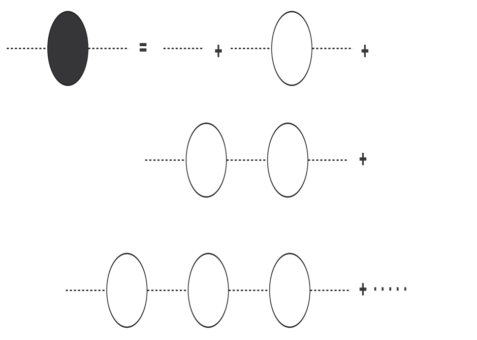
FIG. 2.: Propagator for the auxiliary field in leading order in the large $N$ limit. There is a factor $\sqrt{\lambda\over N}$ for each vertex and a factor $N$ for each bubble. The propagator is of ${\cal O}(1)$ in the large $N$ limit.

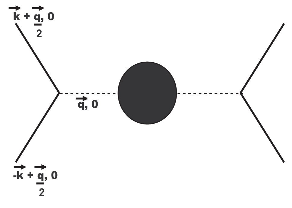
FIG. 3.: Two particle s-channel scattering amplitude in the static and large $N$ limit. $\vec{q},~{}q_{0}=0$ are the transferred momentum and frequency carried by the propagator of the auxiliary field.

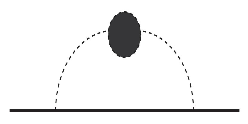
FIG. 4.: The self-energy of the scalar field at order $1/N$.

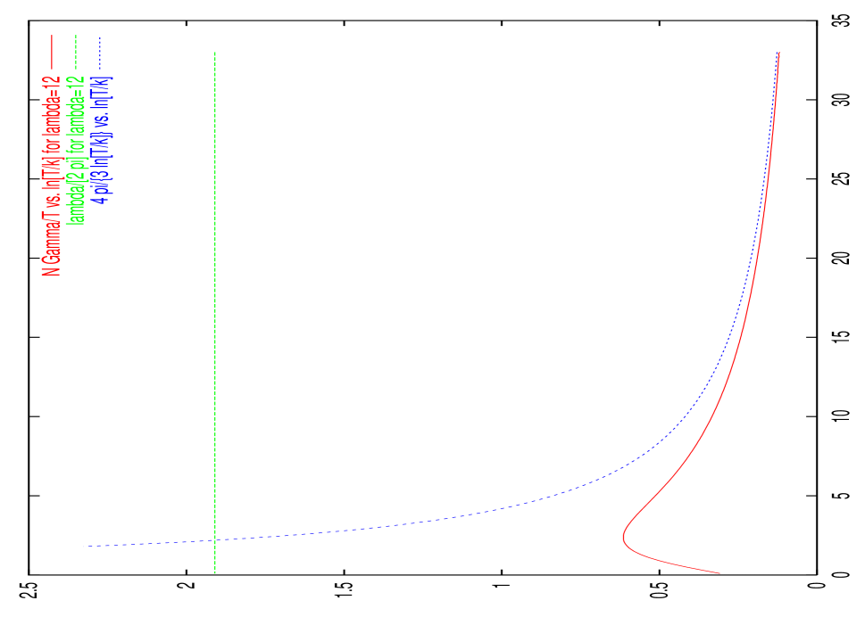
FIG. 5.: $N\;\Gamma(k,T)/T$ vs. $\ln[T/k]$ for $\lambda=12.0$. We also plot the classical value $\lambda/[2\pi]$ and the asymptotic ultrasoft behavior $N\;\Gamma(k,T)/T={4\pi\over 3\ln[T/k]}$. We see in this strong coupling regime that the ultrasoft asymptotics correctly describes the relaxation rate.

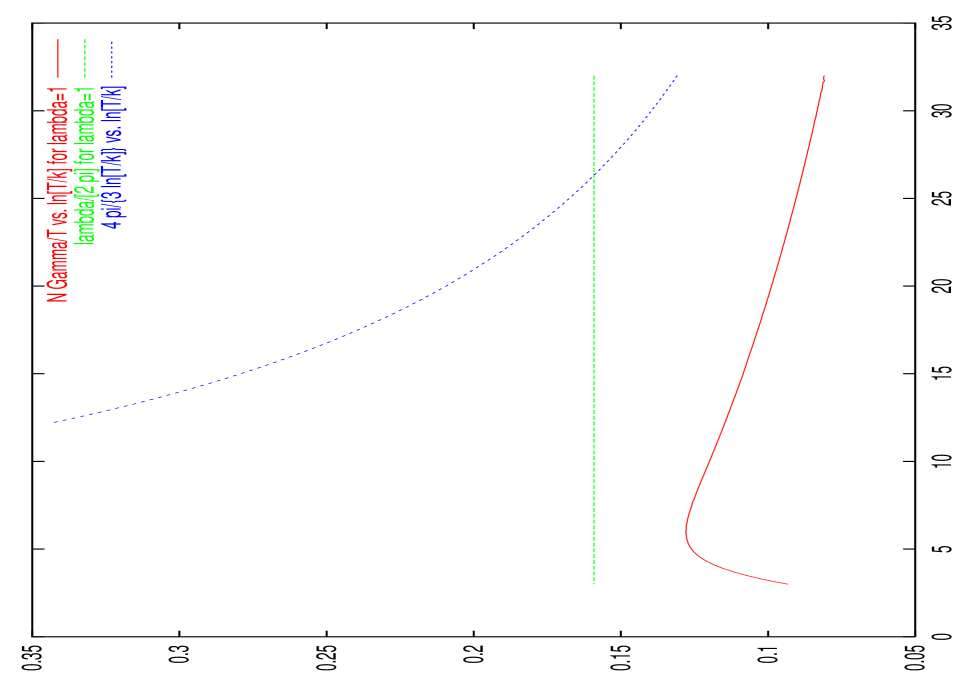
FIG. 6.: $N\Gamma(k,T)/T$ vs. $\ln[T/k]$ for $\lambda=1.0$. We also plot the classical value $\lambda/[2\pi]$ and the asymptotic ultrasoft behavior $N\Gamma(k,T)/T={4\pi\over 3\ln[T/k]}$. For this intermediate coupling regime the classical approximation provides a qualitative a estimate whereas the ultrasoft regime will be reached for $k/T\ll 3.\;10^{-7}$.

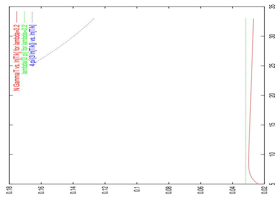
FIG. 7.: $N\;\Gamma(k,T)/T$ vs. $\ln[T/k]$ for $\lambda=0.2$. We also plot the classical value $\lambda/[2\pi]$ and the asymptotic ultrasoft behavior $N\;\Gamma(k,T)/T={4\pi\over 3\ln[T/k]}$. In the small coupling regime the classical approximation describes very well the behaviour of the relaxation rate.The ultrasoft regime will only be reached for extremely small momenta $k/T\ll 8.\;10^{-30}$

FIG. 8.: Damping rate $N\;\Gamma_{0}(m_{T},T)/T$ vs. $\ln[T/m_{T}]$ for homogenous configurations ($k=0,\;T\neq T_{c}$) compared with the classical approximation $N\;\Gamma_{cl}(m_{T},T)/T=\lambda/(2\pi)$ and the asymptotic expression in the medium coupling regime $\lambda=1.0$.

FIG. 9.: Damping rate $N\;\Gamma_{0}(m_{T},T)/T$ vs. $\ln[T/m_{T}]$ for homogenous configurations ($k=0,\;T\neq T_{c}$) compared with the classical approximation $N\;\Gamma_{cl}(m_{T},T)/T=\lambda/(2\pi)$ and the asymptotic expression in the small coupling regime $\lambda=0.2$.

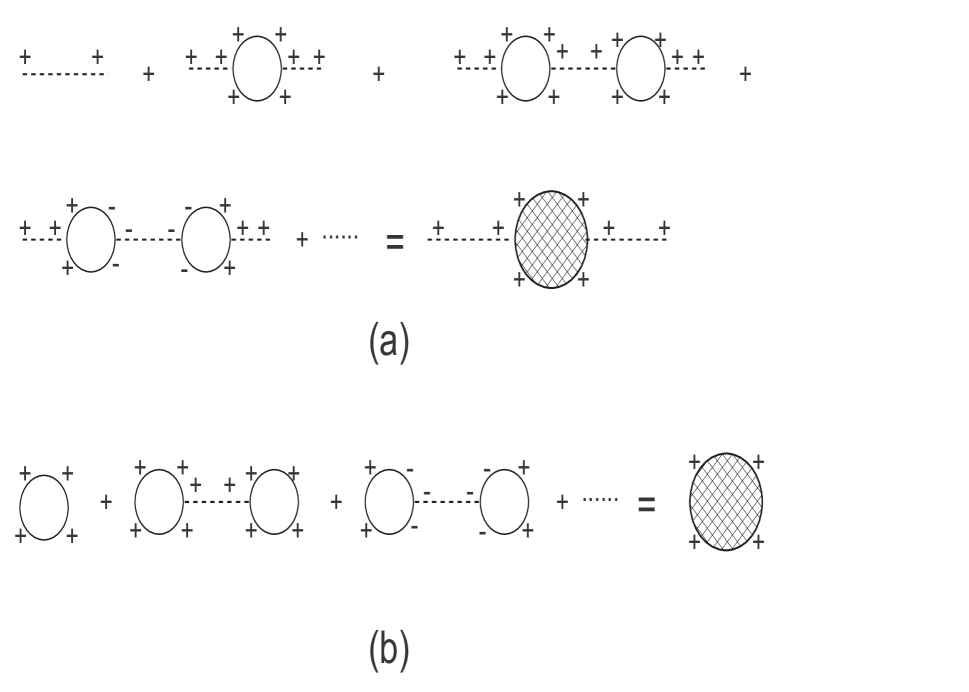
FIG. 10.: (a): Feynman diagrams for the correlator $\langle\chi^{+}(\vec{x},t)\chi^{+}(\vec{x}^{\prime},t^{\prime})\rangle$, (b):Feynman diagrams for the correlator $\langle(\vec{\Phi}^{+}(\vec{x},t))^{2}(\vec{\Phi}^{+}(\vec{x}^{\prime},t^{\prime}))^{2}\rangle$.

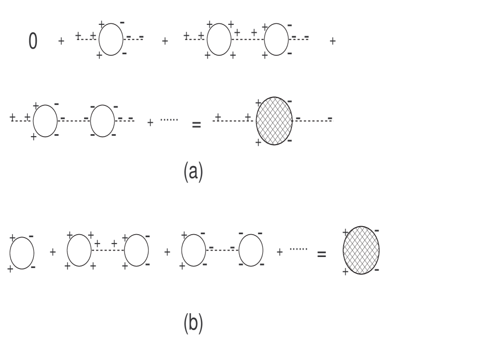
FIG. 11.: (a): Feynman diagrams for the correlator $\langle\chi^{+}(\vec{x},t)\chi^{-}(\vec{x}^{\prime},t^{\prime})\rangle$, (b): Feynman diagrams for the correlator $\langle(\vec{\Phi}^{+}(\vec{x},t))^{2}(\vec{\Phi}^{-}(\vec{x}^{\prime},t^{\prime}))^{2}\rangle$.

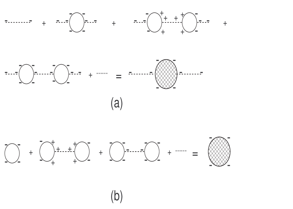
FIG. 12.: (a): Feynman diagrams for the correlator $\langle\chi^{-}(\vec{x},t)\chi^{-}(\vec{x}^{\prime},t^{\prime})\rangle$, (b): Feynman diagrams for the correlator $\langle(\vec{\Phi}^{-}(\vec{x},t))^{2}(\vec{\Phi}^{-}(\vec{x}^{\prime},t^{\prime}))^{2}\rangle$.

REFERENCES

- [1] For recent reviews on the QCD phase transitions and aspects of relativistic heavy ion collisions see for example: J. W. Harris and B. Muller, Annu. Rev. Nucl. Part. Sci. 46, 71 (1996); B. Muller in Particle Production in Highly Excited Matter, Eds. H.H. Gutbrod and J. Rafelski, NATO ASI series B, vol. 303 (1993); B. Muller, The Physics of the Quark Gluon Plasma Lecture Notes in Physics, Vol. 225 (Springer-Verlag, Berlin, Heidelberg, 1985); K. Rajagopal in ‘Quark-Gluon Plasma 2’, Ed. by R. C. Hwa, World Scientific, Singapore, 1995; H. Meyer-Ortmanns, Rev. of Mod. Phys. 68, 473 (1996).
- [2] See the CERN web page for a summary of results from SPS: www.cern.ch/CERN/Announcements/2000/NewStateMatter/ and U. Heinz and M. Jacob, nucl-th/0002042, Evidence for a New State of Matter: An Assessment of the Results from the CERN Lead Beam Programme.
- [3] R. Pisarski and F. Wilczek, Phys. Rev. D29 (1984), 338.
- [4] K. Rajagopal and F. Wilczek, Nucl.Phys. B399 (1993) 395.
- [5] J. Berges and K. Rajagopal, Nucl. Phys. B538 (1999), 215; M. A. Halasz, A. D. Jackson, R.E. Shrock, M. A. Stephanov and J. J. M. Verbaarschot, Phys. Rev. D58 (1998), 096007.
- [6] M. Stephanov, K. Rajagopal and E. Shuryak, Phys. Rev. D60 (1999) 114028; Phys. Rev. Lett. 81 (1998) 4816
- [7] B. Berdnikov and K. Rajagopal, Slowing Out of Equilibrium Near the QCD Critical Point ,hep-ph/9912274.
- [8] Shang-Keng Ma, Modern Theory of Critical Phenomena, (Benjamin Advanced Book Program, Frontiers in Physics, Reading Mass. 1976).
- [9] P. C. Hohenberg and B. I. Halperin, Rev. Mod. Phys. 49 (1977) 435.
- [10] E.V. Shuryak, Phys.Lett. B423 (1998) 9. G.V.Danilov and E.V. Shuryak, On the Origin of the Multiplicity Fluctuations in High Energy Heavy Ion Collisions, nucl-th/9908027.
- [11] D. Forster, Hydrodynamic Fluctuations, Broken Symmetry and Correlation Functions (Addison Wesley, Redwood City, 1990).
- [12] K. Jedamzik, Phys. Rev. D55 (1997), R5871; K. Jedamzik and J. C. Niemeyer, Phys. Rev. D59 (1999), 124014-1.
- [13] C. Schmid, D. J. Schwarz and P. Widerin, Phys. Rev. D59 (1999), 043517-1; Phys. Rev. Lett. 78 (1997), 791.
- [14] S. Banerjee, A. Bhattacharyya, S. K. Goshi and S. Raja, The cosmological quark-hadron transition and massive compact halo objects astro-ph/0002007
- [15] N. Borghini, W. N. Cottingham and R. V. Mau, Possible cosmological implications of the quark-hadron phase transition, hep-ph/0001284.
- [16] H. E. Stanley, Introduction to Phase Transitions and Critical Phenomena (Oxford Univ. Press, New York, 1971).
- [17] For a comparison of phenomenological classical approach to non-equilibrium dynamics and the microscopic quantum field theoretical treatment see for example: D. Boyanovsky and H. J. de Vega, Dynamics of Symmetry Breaking Out of Equilibrium: From Condensed Matter to QCD and the Early Universe, hep-ph/9909372 ; D. Boyanovsky, H. J. de Vega and R. Holman, Non-equilibrium phase transitions in condensed matter and cosmology: spinodal decomposition, condensates and defects, hep-ph/9903534.
- [18] M. Le Bellac, Thermal Field Theory (Cambridge University Press, Cambridge, England, 1996).
- [19] E. Braaten and R.D. Pisarski, Nucl. Phys. B337, 569 (1990); ibid. B339, 310 (1990).
- [20] J.-P. Blaizot and E. Iancu, Nucl. Phys. B459 (1996) 559; Nucl. Phys. B434 (1995) 662.
- [21] P. Arnold and L. G. Yaffe Phys. Rev. D57 (1998) 1178.
- [22] R.R. Parwani, Phys. Rev. D 45, 4695 (1992).
- [23] D. Boyanovsky, H. J. de Vega and R. Holman, Nonequilibrium Dynamics of Phase Transitions: From the Early Universe to Chiral Condensates, Second Paris Cosmology Colloquium: Proceedings. Eds. H. J. de Vega and N. Sanchez, World Scientific, 1995; D. Boyanovsky, D. Cormier, H. J. de Vega, R. Holman, S. P. Kumar, Out of Equilibrium Fields in Inflationary Dynamics: Density Fluctuations In the Proceedings of the VIth. Erice Chalonge School on Astrofundamental Physics, N. Sánchez and A. Zichichi eds., Kluwer, 1998; D. Boyanovsky, H. J. de Vega, R. Holman, Erice Lectures on Inflationary Reheating in the Proceedings of the 5th. Erice Chalonge School on Astrofundamental Physics, N. Sánchez and A. Zichichi eds., (World Scientific, 1997);D. Boyanovsky, M. D’Attanasio, H. J. de Vega, R. Holman, and D.-S. Lee, Phys. Rev. D52, 6805 (1995); New Aspects of Reheating, String Gravity and Physics at the Planck Energy Scale: Proceedings of the NATO ASI at Erice, Italy, p.451, Eds. N. Sanchez and A. Zichichi, Kluwer, 1996.
- [24] G. Aarts and J. Smit, Nucl. Phys. B511 (1998) 451; Phys.Lett. B393 (1997) 395
- [25] W. Buchmuller and A. Jakovac, Nucl. Phys. B521 (1998) 219; Phys.Lett. B407 (1997) 39.
- [26] F. Cooper, S. Habib, Y. Kluger, E. Mottola, J. P. Paz, and P. R. Anderson, Phys. Rev. D50, 2848 (1994); F. Cooper, Y. Kluger, E. Mottola, and J. P. Paz, Phys. Rev. D51, 2377 (1995).
- [27] I. S. Gradshteyn and I. M. Ryshik, Table of Integrals, Series and Products, Academic Press, New York, 1980.
- [28] D. Boyanovsky, I. D. Lawrie, D. S. Lee, Phys. Rev. D54 (1996) 4013
- [29] M. Pietroni, Phys.Rev.Lett. 81 (1998) 2424.
- [30] B. Bergerhoff and J. Reingruber, A consistent nonperturbative approach to thermal damping-rates , hep-ph/0004039.