BCP3: Summary of Theory

Abstract

I discuss a number of the highlights in theory presented at the BCP3 conference. These included new, and more stringent, CKM fits; a critical overview of heavy hadron lifetimes; progress in computing rates and CP-asymmetries in charmless B-decays; a thorough discussion of the implications of the new results on $\epsilon^{\prime}/\epsilon$; and, finally, a peek at the future, trying to estimate how well one is going to be able to measure the unitarity triangle angles.

It is, as usual, very difficult to summarize the myriad of talks in a conference dedicated to a forefront topic in particle physics. BCP3 was no exception. Thus here, asking the indulgence of the speakers whose work I will not mention, I will only touch on a few of the highlights in theory which I thought were particularly interesting.

1 CKM Fits: Where Do We Stand?

During BCP3 there was much discussion of how well we can determine the parameters in the CKM matrix. In practice, this means finding the allowed region, at a certain confidence level, in the $\rho-\eta$ plane - with $\rho$ and $\eta$ being the usual Wolfenstein $\!{}^{{\bf?}}$ parameters. The ingredients of the global fits discussed here particularly by Stocchi $\!{}^{{\bf?}}$, as well as by Kim $\!{}^{{\bf?}}$ and Eigen $\!{}^{{\bf?}}$, are crucially dependent on the errors one assigns to the values one infers experimentally for $|V_{ub}|$ and $|V_{cb}|$.  $\!{}^{{\bf?}}$ $\!{}^{{\bf?}}$ Although the data on $\sin 2\beta$ coming from the Tevatron $\!{}^{{\bf?}}$, and now also from ALEPH,  $\!{}^{{\bf?}}$ $\!{}^{{\bf?}}$ is not accurate enough to have much impact on the allowed region in the $\rho-\eta$ plane, the sharpened LEP bound on $\Delta m_{s}$, presented here by Willocq,  $\!{}^{{\bf?}}$ provides a significant restriction.

When considering the result of the CKM fits, it is important to distinguish three different ingredients that enter into these fits

i) There are a number of experimental inputs which have quite negligible experimental errors. These include: the CP-violating parameter $|\epsilon|$; the $B_{d}-\bar{B}_{d}$ mass difference, $\Delta m_{d}$; the $\Delta m_{s}$ bound mentioned above;  $\!{}^{{\bf?}}$ and the value of the sine of the Cabibbo angle, $\sin\theta_{C}\equiv\lambda$.

ii) There are a number of parameters which have, what one may call controllable errors. These include $|V_{cb}|$ ; the ratio $|V_{ub}|/|V_{cb}|$ and the $SU(3)$-breaking parameter $\xi=f_{B_{s}}{\sqrt{B_{B_{s}}}}/f_{B_{d}}{\sqrt{B_{B_{d}}}}$.

iii) There are also associated theoretical parameters, whose errors are due to theoretical uncertaintes in determining appropriate hadronic matrix elements. These include $B_{K}$, the parameter which measures how different the matrix element $<K|({\bar{d}}s)^{2}_{V-A}|{\bar{K}}>$ is from the vacuum saturation result $(B_{K}=1)$; and the analogous parameter for the $B_{d}$ system, $B_{d}f_{B_{d}}^{2}$, which is connected to the matrix element $<B_{d}|({\bar{d}}b)^{2}_{V-A}|{\bar{B}}_{d}>$.

The parameters with controllable errors, in principle, are the ones which can be improved using more experimental information.  In contrast, it is difficult to reduce, or even correctly estimate, the theoretical errors associated with parameters like $B_{K}$, because they are connected with the way one attempts to calculate the hadronic matrix elements. Although Soni $\!{}^{{\bf?}}$ in this meeting has given 15% errors on $B_{K}$ and $f_{B_{d}}{\sqrt{B_{B_{d}}}}$ $[B_{K}=0.85\pm 0.13$; $f_{B_{d}}{\sqrt{B_{B_{d}}}}=(230\pm 30)MeV]$, the systematic error on each of these quantities is much harder to pin down, since it depends on the uncertainties associated with going from a quenched to a fully unquenched calculation of the relevant matrix elements.

The fit of Stocchi shown in Fig. 1 uses the parameters detailed in Table 1. Although I find this set of parameters (and the fit!) perfectly reasonable, I believe that one should not take the 95% confidence limit region shown in Fig. 1 strictly as such. There is enough ”theoretical error” in this whole business that the most prudent approach is to transform a ”formal” 95% confidence limit region into an ”effective” 68% limit region. Even after doing such an unorthodox thing, one cannot but be impressed by how well the CKM model fits the data!

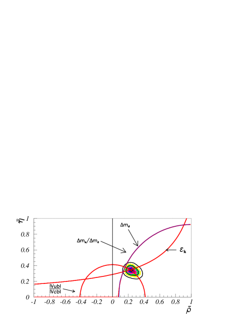
Figure 1: CKM fit presented in Ref [2].

Table 1: Input parameters for the fit in Fig. 1, from reference [2]

Parameter	Value
$|\epsilon|$	$(2.280\pm 0.019)\times 10^{-3}$
$|V_{ub}|/|V_{cb}|$	$0.080\pm 0.006\pm 0.016$  Cornell
$|V_{ub}|/|V_{cb}|$	$0.104\pm 0.012\pm 0.015$   LEP
$\Delta m_{d}$	$(0.472\pm 0.016)~{}{\rm ps}^{-1}$
$\Delta m_{s}$	$>14.3~{}{\rm ps}^{-1}$
$|V_{cb}|$	$(40.4\pm 1.9)\times 10^{-3}$
$B_{K}$	$0.86\pm 0.06\pm 0.08$
$f_{B_{d}}{\sqrt{B_{B_{d}}}}$	$(210\pm 29\pm 12)$MeV
$\xi$	$1.11\pm 0.02\pm 0.05$

As I mentioned earlier, the new result from LEP reported here by Willocq $\!{}^{{\bf?}}$ on the $B_{s}-\bar{B}_{s}$ mass difference is of considerable importance for the final $\rho-\eta$ plane fit. Last year this parameter was bounded a bit more weakly $(\Delta m_{s}>12.4~{}{\rm ps^{-1}})$ so that the final $\rho-\eta$ plane fit permitted values of $\rho<0$.  $\!{}^{{\bf?}}$ With the present bound, however, one cannot contemplate any longer negative values for $\rho$— a point emphasized by Deshpande $\!{}^{{\bf?}}$ at this meeting. If $\rho>0$, it follows that the CKM CP-violating phase $\gamma$ cannot be as large as $90^{0}$. In turn, this implies that one cannot any longer contemplate the superweak solution for the unitarity triangle angles $\alpha$ and $\beta$, in which $\sin 2\beta=\sin 2\alpha$. Indeed, the fit of the CKM parameters presented by Stocchi here leads to a best value for $\sin 2\beta$ and $\sin 2\alpha$ which are quite different from each other:  $\!{}^{{\bf?}}$

$$\sin 2\beta=0.75\pm 0.06:~{}~{}\sin 2\alpha=-0.22\pm 0.24~{}.$$ (1)

I remark, that the 95% confidence limit on $\sin 2\beta$ which one infers from the CKM analysis,

$$0.62\leq\sin 2\beta\leq 0.88,$$ (2)

is precisely in the range determined by present experiments. The value reported here for $\sin 2\beta$, obtained by ALEPH  $\!{}^{{\bf?}}$  $\!{}^{{\bf?}}$

$$\sin 2\beta=0.93^{+0.64~{}+0.36}_{-0.88~{}-0.24}~{},$$ (3)

when combined with the CDF result $\!{}^{{\bf?}}$ [$\sin 2\beta=0.79^{+0.41}_{-0.44}$], leads to an average value

$$<\sin 2\beta>=0.91\pm 0.35~{},$$ (4)

which is perfectly compatible with the range for $\sin 2\beta$ obtained indirectly from the CKM analysis. Furthermore, this experimental result, by itself, is already almost significant statistically.

It is possible to imagine improving considerably the allowed value for $\sin 2\beta$ and other unitarity triangle parameters by improving the controllable errors on $|V_{ub}|/|V_{cb}|$ and on the other parameters which enter in the CKM analysis. Let me illustrate how these improvements can come about by focusing specifically on the case of $|V_{cb}|$. If one could trust the parton model, and one knew the mass of the b-quark precisely, one could directly extract $|V_{cb}|$ from the semileptonic width for b-quarks to decay into final states containing c-quarks, given by the standard formula:

$$\Gamma(b\to c\ell{\bar{\nu}}_{e})=|V_{cb}|^{2}\frac{G^{2}_{F}}{192\pi^{3}}m^{5}_{b}~{}.$$ (5)

This formula, however, is of no use since $m_{b}$ itself is not known precisly enough and, furthermore, there are corrections to the parton model!

What one does, in practice, is to use the Heavy Quark Effective Theory (HQET) to replace $m_{b}$ by the mass of the B-meson. In so doing the rate (5) above is corrected by the addition of terms involving the matrix elements of the operators $0_{i}$ which enter in the operator produced expansion underlying the HQET.  $\!{}^{{\bf?}}$ To $0(1/m_{b}^{2})$ one has two new operators contributing to the total width, which are characterized by two parameters $\lambda_{1}$, and $\lambda_{2}$ given by

$$\lambda_{1} = \frac{1}{2M_{B}}<B|{\bar{b}}(iD)^{2}b|B>$$ (6)

$$\lambda_{2} = \frac{g_{3}}{2M_{B}}<B|{\bar{b}}\sigma_{\mu\nu}G^{\mu\nu}b|B>~{},$$

where $G^{\mu\nu}$ is the gluon field strength tensor. In addition, to this order in the heavy quark expansion,  $\!{}^{{\bf?}}$ the Fermi momentum ${\bar{\Lambda}}$ enters in the formulas relating the mass of the b-quark to that of the $B$ and $B^{*}$ mesons:

$$M_{B} = m_{b}+{\bar{\Lambda}}-\frac{(\lambda_{1}+3\lambda_{2})}{m_{b}}$$ (7)

$$M_{B}^{*} = m_{b}+{\bar{\Lambda}}-\frac{(\lambda_{1}-\lambda_{2})}{m_{b}}~{}.$$

Using the physical masses for $M_{B}$ and $M_{B}^{*}$ yields directly a value for $\lambda_{2}~{}[\lambda_{2}\simeq 0.12~{}{\rm GeV}^{2}]$.

Using the heavy quark expansion one can obtain a formula for the semileptonic rate $\Gamma(B\to X_{c}\ell\bar{\nu}_{\ell})$ which involves $M_{B}$ rather than $m_{b}$, at the price of some corrections involving $\lambda_{1},\lambda_{2}$, and ${\bar{\Lambda}}$. One finds, including leading order QCD effects, $\!{}^{{\bf?}}$ the formula:

$$\Gamma(B\to X_{c}\ell{\bar{\nu}}_{\ell}) = |V_{cb}|^{2}\frac{G^{2}_{F}}{192\pi^{3}}M_{B}^{5}\Phi(\frac{M_{D}}{M_{B}})[1-1.54\frac{\alpha_{s}}{\pi}+...]$$

$$\cdot \{1-1.65\frac{{\bar{\Lambda}}}{M_{B}}\ -3.18\frac{\lambda_{1}}{M_{B}^{2}}+0.02\frac{\lambda_{2}}{M_{B}^{2}}+...\}~{}.$$

Here $\Phi(M_{D}/M_{B})$ is a phase space factor, while the first square bracket contains the $0(\alpha_{s})$ perturbative QCD corrections. The terms in the curly brackets are the dominant corrections coming from the heavy quark expansion. If, besides $\lambda_{2}$, one knew $\lambda_{1}$ and ${\bar{\Lambda}}$ with good accuracy, one could determine $|V_{cb}|$ from the semileptonic width with a small $0(1/m_{b}^{3})$ theory error. The parameters $\lambda_{1},\lambda_{2}$, and ${\bar{\Lambda}}$ are, in principle, controllable since they can be inferred from properties of the lepton spectrum and of the hadronic mass spectrum in non-leptonic $B$-decays . $\!{}^{{\bf?}}$ Specifically, moments of the lepton spectrum and/or the hadronic mass spectrum can be used to determine $\lambda_{1}$ and ${\bar{\Lambda}}$.

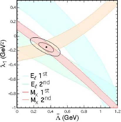
Figure 2: Preliminary analysis by the CLEO Collaboration of the moments of the hadronic mass spectrum (dark shaded) and moments of the leptonic energy spectrum (light shaded) to determine $\lambda_{1}$ and $\bar{\Lambda}$.

Unfortunately, as shown in Fig. 2, a preliminary analysis by the CLEO collaboration — presented here by Thaler $\!{}^{{\bf?}}$ — give inconsistent results. The values for $\lambda_{1}$ and ${\bar{\Lambda}}$ determined from the leptonic spectrum do not seem to agree with those computed from an analysis of the moments of the hadronic mass spectrum. In my view, the latter values $[\lambda_{1}=(-0.13\pm 0.01\pm 0.06)~{}{\rm GeV^{2}}$;  ${\bar{\Lambda}}=(0.33\pm 0.02\pm 0.08)$  GeV] are probably more trustworthy, since they are less sensitive to some of the necessary experimental cuts. Indeed, these values are quite close to the values reported by W. M. Zhang $\!{}^{{\bf?}}$ at this meeting, coming from a B-bound state analysis using an explicit phenomenological wavefunction for the B-meson. At any rate, using these techniques, it is likely that one will be able to eventually reduce the theoretical error on $|V_{cb}|$ to about $1\times 10^{-3}~{}(2.5\%)$ and on $|V_{ub}|$ to about $4\times 10^{-4}~{}(10\%)$, with a corresponding reduction of the allowed region in the $\rho-\eta$ plane. As Misiak $\!{}^{{\bf?}}$ discussed in BCP3, this same approach can be used in other contexts — in particular, to better constrain the dependence on the photon energy of the branching ratio for $B\to X_{s}\gamma$ above some minimum photon energy cut.

2 Lifetimes of Heavy Hadrons

There is reasonable theoretical understanding of the specific pattern of lifetimes of heavy hadrons containing $c$ and $b$ quarks. This topic was reviewed here by Bigi  $\!{}^{{\bf?}}$ and specific aspects were considered by Melic  $\!{}^{{\bf?}}$ and by Yang  $\!{}^{{\bf?}}$. However, as the data on these lifetimes is now rather precise,  $\!{}^{{\bf?}}$ a puzzle has emerged. I want to discuss this briefly here.

One can understand the total decay width – and hence the lifetime – of a heavy hadron theoretically via the HQET. The total width is given by the discontinuity of the correlator of the weak Hamiltonian responsible for the decay with itself. This discontinuity is given by a sum of matrix elements of operators of increasing dimensonality, arising in an operator product expansion of the correlator. Schematically, one finds in this way the formula $\!{}^{{\bf?}}$

$$\Gamma_{\rm tot}\sim G_{F}^{2}m_{Q}^{5} \left[<H_{Q}|\bar{Q}Q|H_{Q}>+{\frac{C_{g}}{m_{Q}^{2}}}<H_{Q}|\bar{Q}\sigma_{\mu\nu}G^{\mu\nu}Q|H_{Q}>\right.$$

$$\left.+{\frac{C_{4f}}{m_{Q}^{3}}}<H_{Q}|\bar{Q}\Gamma q\bar{q}\Gamma Q|H_{Q}>+...\right]~{},$$

where $m_{Q}$ is the mass of the heavy quark. As can be gleaned from the above, the expansion parameter for the total width is of order $\Lambda_{QCD}/m_{Q}$. Hence one expects that the effects of the non-leading terms in Eq. (9) should be bigger in charm decays than in bottom decays. Indeed, experimentally $\tau(D^{+})/\tau(D^{o})\sim 2.5$ while the $B^{+}$ and $B^{o}_{d}$ lifetimes are nearly equal $[\tau(B^{+})/\tau(B^{o}_{d})=1.066\pm 0.024$  $\!{}^{{\bf?}}$]

More specifically, the situation regarding the decays of charmed hadrons seems rather satisfactory.  $\!{}^{{\bf?}}$ The dominant effect that causes the large difference between the lifetimes of the $D^{+}$ and $D^{0}$ mesons can be traced to the Pauli interference  $\!{}^{{\bf?}}$ originating from the 4-fermion term in Eq. (9). These 4-fermion terms are also crucial to explain the pattern of charmed baryon lifetimes, as detailed by Melic  $\!{}^{{\bf?}}$ at this meeting. The fact that $\tau(D_{s})/\tau(D^{o})$ is near to 1.2  $[\tau(D^{o})=408\pm 4.1~{}{\rm fs};~{}\tau(D_{s})=486\pm 15~{}{\rm fs}$ $\!{}^{{\bf?}}$] is probably evidence for some weak annihilation contribution $(c{\bar{s}}\to W^{+})$ in the $D_{s}$ width.  $\!{}^{{\bf?}}$ If so, perhaps one should be able to see some evidence for glueball or $\eta^{\prime}$ decays of the $D_{s}$, processes like $D_{s}\to$ glueball $\ell{\bar{\nu}}_{\ell}$ ; $D_{s}\to\eta^{\prime}\ell{\bar{\nu}}_{\ell}$.

Although the prediction that the lifetime differences in the $B$-sector should be small is well borne out by the data, there is a nagging problem with the $\Lambda_{b}$ lifetime.  $\!{}^{{\bf?}}$ The Pauli interference effects suppress the lifetime of the $\Lambda_{b}$ relative to that of the $B_{d}$-meson and one can write

$$\frac{\tau(\Lambda_{b})}{\tau(B_{d})}=1-\Delta$$ (10)

Bigi $\!{}^{{\bf?}}$ estimates $\Delta\simeq 0.05$, while Melic  $\!{}^{{\bf?}}$ can push $\Delta$ to perhaps $\Delta\simeq 0.1$ by taking a very light $b$-quark mass. However, experimentally this ratio is closer to 0.8, with the latest results giving $\tau(\Lambda_{b})/\tau(B_{d})=0.79\pm 0.05$.  $\!{}^{{\bf?}}$ It is possible that this signals a real discrepancy between theory and experiment that needs explaining. However, in my view, given the fine agreement of all the other heavy hadron lifetimes with the predictions coming from HQET, perhaps one should not worry overmuch at this stage about a (2-3) $\sigma$ discrepancy. Hopefully, future data from the Tevatron should help resolve this issue.

3 Charmless $B$-decays: Rates and CP-Asymmetries

At BCP3 there was lots of discussion of 2-body charmless $B$-decay. Data on these decays was presented by J. Smith  $\!{}^{{\bf?}}$ and J. Alexander  $\!{}^{{\bf?}}$, while various theoretical aspects were touched upon by H-Y Cheng  $\!{}^{{\bf?}}$; C. D. Lu $\!{}^{{\bf?}}$, H.-n. Li $\!{}^{{\bf?}}$, M. Suzuki  $\!{}^{{\bf?}}$and C. Bhattacharya.  $\!{}^{{\bf?}}$

H.- Y. Cheng $\!{}^{{\bf?}}$ in particular, summarized the recent considerable progress achieved in calculating within QCD the relative rates for the decays of $B$-meson into 2 pseudoscalar states $[B\to PP]$, 2 vector states $[B\to VV]$ and a vector and a pseudoscalar state $[B\to VP]$ . The present treatment formalizes (and, in a sense, justifies and explains) the old diagrammatic approach to this problem of Ling Lie Chau.  $\!{}^{{\bf?}}$ The basic idea of these calculations is well known. One starts with an effective weak Hamiltonian given by a sum of operators

$$H_{\rm eff}=\sum_{i}C_{i}(\mu)0_{i}(\mu)~{},$$ (11)

and one tries to estimate the matrix elements of these operators by using factorization. However, then one correct this procedure by including (some) non-factorizable pieces.

Technically, when one uses factorization, in the process of splitting up the operators as a product of currents the scale dependence of the matrix elements of $0_{i}(\mu)$ is not preserved:

$$<M_{1}M_{2}|0_{i}(\mu)|B>=<M_{1}|J_{i}|B><M_{2}|J_{i}|B>~{}.$$ (12)

However, one can reorganize the Wilson coefficient expansion  $\!{}^{{\bf?}}$ to effectively recover $\mu$-independent coefficients $C^{\rm eff}_{i}$ - at least to $0(\alpha_{s})$. For Penguin operators these effects are rather large, amounting to about a $50\%$ increase for $C^{\rm eff}_{6}$. $\!{}^{{\bf?}}$ Non-factorizable contributions are incorporated as $1/N_{c}$ corrections. As Cheng $\!{}^{{\bf?}}$ discussed, the recent advance comes from understanding that, depending on which operator $0_{i}$ one is considering, the correction factors have different $N_{c}$-factors associated with them . This has been justified in the heavy quark limit recently by Beneke, Buchalla, Neubert and Sachrajda. $\!{}^{{\bf?}}$ In particular, for $(V-A)(V-A)$ operators $N^{\rm eff}_{c}\simeq 2$, while for $(V+A)(V-A)$ operators $N_{c}^{\rm eff}\simeq 6$.

H.- Y. Cheng $\!{}^{{\bf?}}$ compared the theoretical predictions resulting from the above considerations with experimental results. The overall comparison is quite good, but there are two extant problems. These are:

i) It is difficult to get the branching ratio $BR(B\to KK)\simeq 0.25BR(B\to K\pi)$ as is observed experimentally. Typically, one finds much larger $B\to\pi\pi$ branching fractions than are observed.

ii) It is very hard to push the $BR(B\to\eta^{\prime}K)$ to the very large level observed $(BR\sim 80\times 10^{-6})$ Typically, theoretically one can reach at most $BR(B\to\eta^{\prime}K)\sim 50\times 10^{-6}$. In fact, to get to values as large as this, it is necessary that $N^{\rm eff}_{c}=2$ for $(V-A)(V-A)$ operators, as is suggested theoretically.

J. Smith $\!{}^{{\bf?}}$ discussed a, theoretically less sophisticated, fit of the measured charmless $B$-decays. In this fit, which was carried out by Hou, Smith and W$\ddot{\rm u}$rtheim,  $\!{}^{{\bf?}}$ one simply considers the amplitude for the B-decays in question to be given by a Tree plus a Penguin contribution, neglecting throughout any strong rescattering phases. Further, these authors use (naive) factorization to calculate the relevant matrix elements. Since the Tree amplitudes depended on the CKM phase $\gamma$ $[T=|T|e^{-i\gamma}]$, this fit determines this phase. Remarkably the fit discussed by Smith $\!{}^{{\bf?}}$ determines $\gamma$ quite accurately:

$$\gamma=(114^{+25}_{-21})^{o}~{}.$$ (13)

However, it is difficult to judge the reliability of the approach. Furthermore, also in this case the branching fraction for the decay $B\to\eta^{\prime}K$ is too low  $[BR(B\to\eta^{\prime}K)\sim 30\times 10^{-6}]$.

The situation regarding direct CP-asymmetries is much less clear, both experimentally and theoretically, Experimentally, as Alexander  $\!{}^{{\bf?}}$ indicated, one is statistics limited so that $\delta A_{\rm CPviol.}$ is typically of $0(0.2)$. For example, one has  $\!{}^{{\bf?}}$

$$A_{\rm CPviol.}(K^{\pm}\pi^{\mp}) = -0.04\pm 0.16$$ (14)

$$A_{\rm CPviol.}(K^{0}\pi^{\pm}) = +0.18\pm 0.24$$

Improvements will scale as $1/\sqrt{N}$ and one will need an integrated luminosity of $0(100~{}{\rm fb}^{-1})$ to get to $\delta A_{\rm{CPviol.}}\simeq 0.04!$

Theoretically to be able to predict these direct CP-asymmetries one needs a good estimate of the strong rescattering phases. If one writes for the amplitudes of two charge -conjugate processes

$$T=T_{1}+T_{2}e^{i\delta_{w}}e^{i\delta_{s}};~{}~{}{\bar{T}}=T_{1}+T_{2}e^{-i\delta_{w}}e^{i\delta_{s}}~{},$$ (15)

one sees that $A_{{\rm CPviol.}}$ vanishes if there is no strong rescattering phase $\delta_{s}$ between the two amplitudes:

$$A_{{\rm CPviol.}}=\frac{2r\sin\delta_{w}\sin\delta_{s}}{1+r^{2}+2r\cos\delta_{w}\cos\delta_{s}}~{},$$ (16)

where $r=T_{1}/T_{2}$. For sizeable effects, in addition to having a non-negligible rescattering phase, one needs a relatively large weak CP-violating phase $\delta_{w}$ (which is probably OK in the CKM model) and a ratio $r\sim 1$. Since, typically, the two amplitudes involved are Penguin and Tree amplitudes, one needs these amplitudes to be comparable in size and to have a large rescattering phase between them — not too likely a possibility! Numerically, for example, if $r=0.25,\delta_{w}\equiv\gamma=60^{o}$ and $\delta_{s}=30^{o}$, one obtains $A_{{\rm CPviol.}}\simeq 0.1$.

At BCP3 three different approaches were discussed to try to estimate the rescattering phases $\delta_{s}$ which one might expect. All three approaches have some inherent difficulties, demonstrating how challenging really it is to have a reliable estimate for $\delta_{s}$. C. D. Lu $\!{}^{{\bf?}}$ used the old idea of Bander, Silverman and Soni $\!{}^{{\bf?}}$ to extract a rescattering phase simply from the phase associated with the discontinuity of Penguin graphs. This phase depends on the momentum transfer carried by the gluon, $\delta_{s}(k^{2})$. However, since the relevant $k^{2}$ are rather low, it is natural to question whether one can trust the discontinuity calculated in a pure quark picture to such values of $k^{2}$. In contrast, H.-n. Li $\!{}^{{\bf?}}$ in his talk at BCP3 estimated $\delta_{s}$ as the rescattering phase which emerges in the Brodsky-Lepage bound state formalism  $\!{}^{{\bf?}}$ by means of factorization. In this case, the question is whether one can really use these techniques given the large energy release in the decay process $B\to M_{1}M_{2}$.

Mahiko Suzuki $\!{}^{{\bf?}}$ presented a more general discussion of the problem based on hadronic methods. He argued, I believe correctly, that it is really difficult to apply perturbative QCD ideas — even if one includes some resummation — for the process at hand, since the effective scale is only of order $k_{\rm eff}\sim\sqrt{\Lambda_{QCD}m_{b}}\sim 1.5$ GeV. However, Suzuki also pointed out that the rescattering phase $\delta_{s}$ is also difficult to estimate by hadronic methods. This is because the phase associated with, say, the $|K\pi>$ final state is not simply the phase associated with elastic $K\pi$ scattering. For the energies in question

$$|K\pi>=\sum_{f}e^{i\delta_{f}}|\alpha_{f}>~{},$$ (17)

and most of the states that contribute in the above sum are inelastic (roughtly 80%). Given this fact, Suzuki tried to estimate the effective phase $\delta_{s}$ that emerges by using a random phase approximation. Using this approximation, he was able to correlate the resulting phase $\delta_{s}$ with the elasticity of the process, with the result depending on how favored or disfavored is the factorization of the amplitude. When factorization is not favoreda $\delta_{s}$ is bigger. However, if one really has a large rescattering phase $\delta_{s}$ there are also sizable distorsions of the amplitude — a result which Suzuki $\!{}^{{\bf?}}$ points out was first understood by Fermi! Basically, not only is there a change in the imaginary part associated with the amplitude, but also the real part is affected:

$$T\to T{\rm exp}\left[\frac{P}{\pi}\int\frac{ds^{\prime}\delta_{s}(s^{\prime})}{s^{\prime}-s}\right]~{}.$$ (18)

These considerations make it unlikely that one will be able to really ever get a reliable theoretical prediction for a direct CP-asymmetry. However, this fact should not discourage experimentalists from looking for such CP-asymmetries.

4 Imputs from the Strange Quark Sector

In the last year, the new results on $\epsilon^{\prime}/\epsilon$ announced by KTeV $\!{}^{{\bf?}}$ and by the NA48 Collaboration $\!{}^{{\bf?}}$ have generated an enormous amount of interest. Not surprisingly, this subject was also a topic of considerable discussion at BCP3.

4.1 $\epsilon^{\prime}/\epsilon$ Results and their Interpretation

In BCP3 the experimental situation regarding $\epsilon^{\prime}/\epsilon$ was reviewed by A. Roodman $\!{}^{{\bf?}}$ and by A. Nappi $\!{}^{{\bf?}}$, while the theoretical aspets of these recent results were discussed by Bertolini, $\!{}^{{\bf?}}$ Soni, $\!{}^{{\bf?}}$ Masiero, $\!{}^{{\bf?}}$ and Soldan. $\!{}^{{\bf?}}$ In my view, the nicest aspect of the new KTEV/NA48 results is that they resolve the discrepancy that existed betwen the old Fermilab result, coming from the E731 experiment, $\!{}^{{\bf?}}$ and the results of the old CERN experiment NA31.  $\!{}^{{\bf?}}$ The present results for $\epsilon^{\prime}/\epsilon$:

$${\rm Re}~{}\epsilon^{\prime}/\epsilon=\left\{\begin{array}[]{c}(28.0\pm 4.1)\times 10^{-4}~{}~{}{\rm Ref~{}[35]}\\ (18.5\pm 7.3)\times 10^{-4}~{}~{}{\rm Ref~{}[36]}\end{array}\right.$$ (19)

when combined with the E731 and NA31 results lead to a world average value for this quantity:

$$<{\rm Re}~{}\epsilon^{\prime}/\epsilon>=(21.2\pm 4.6)\times 10^{-4}~{},$$ (20)

which clearly establishes the existence of $\Delta S=1$ CP-violation. This result provides the first direct confirmation that $\sin\gamma\not=0$ or, equivalently, that $\eta\not=0$— something which could only be inferred from the CKM analysis we discussed earlier.

This said, however, it is difficult to extract from the present measurement of $\epsilon^{\prime}/\epsilon$ a precise value for $\eta$. This is because the value of $\epsilon^{\prime}/\epsilon$, although proportional to $\eta$, is rather uncertain due to uncertainties in the calculation of the relevant hadronic matrix element. This point was emphasized by Bertolini $\!{}^{{\bf?}}$ at this meeting. His argument can be illustrated by making use of an approximate formula for $\epsilon^{\prime}/\epsilon$ due to Buras and his collaborators. $\!{}^{{\bf?}}$ As is well known, both matrix elements of gluonic Penguin operators and of electroweak Penguin operators contribute to the process $s\to d{\bar{q}}q$. Although the gluonic Penguin contributions are of $0(\alpha_{s})$, and hence enhanced with respect to the electroweak Penguin contributions which are of $O(\alpha)$, they are suppressed by the $\Delta I=1/2$ rule since they are proportional to $A_{2}/A_{0}$.  $\!{}^{{\bf?}}$ The electroweak Penguin contributions, on the other hand, although naturally small do not suffer from the $\Delta I=1/2$ suppresion and, furthermore, are enhanced by a factor of $m_{t}^{2}/M_{W}^{2}$. $\!{}^{{\bf?}}$ As a result, for $\epsilon^{\prime}/\epsilon$ both Penguin operator contributions are of a similar magnitude and, because they enter with opposite sign, they render the theoretical value for this quantity rather uncertain.

This can be appreciated quite nicely from the approximate formula for $\epsilon^{\prime}/\epsilon$ derived by Buras and his collaborators. $\!{}^{{\bf?}}$ One has

$$\epsilon^{\prime}/\epsilon\simeq 34\eta\left[B_{6}^{1/2}-0.53B_{8}^{1/2}\right]\left(\frac{110MeV}{m_{s}(2GeV)}\right)^{2}\times 10^{-4}~{}.$$ (21)

Here $B_{6}$ and $B_{8}$ are the matrix elements of the gluonic Penguin operator and of the electroweak Penguin operator, respectively — normalized so that in the vacuum insertion approximation $B_{6}=B_{8}=1$. Because, as we have seen, $\eta\simeq 0.3$, the above formula in this approximation gives $\epsilon^{\prime}/\epsilon\sim 5\times 10^{-4}$, which is much below the value measured by KTeV and NA48. Indeed, to get agreement with the present world average [cf Eq. (20)], one needs to stretch all the parameters in Buras’s formula. Namely, one needs to maximize $\eta$ [ $\eta\simeq 0.4]$; decrease the value one assumes for $m_{s}(2GeV)$ [perhaps to $m_{s}$ as low as $m_{s}(2GeV)\simeq 90$ MeV]; increase $B_{6}^{1/2}$ from unity — something which is not clear one can obtain in lattice calculations,  $\!{}^{{\bf?}}$ but which appears to be true in the chiral quark model $\!{}^{{\bf?}}$; and decrease $B_{8}^{1/2}$ — something which emerges naturally both in lattice and $1/N$ calculations. $\!{}^{{\bf?}}$

In this meeting, Bertolini $\!{}^{{\bf?}}$ emphasized that what improves the post-dictions of $\epsilon^{\prime}/\epsilon$ is to incorporate in the calculation the trend observed in the chiral quark model and in the $1/N$ approximation that $B_{6}^{1/2}/B_{8}^{1/2}\simeq 2$, and not unity as expected in the vacuum insertion approximation. However, this is just a phenomenological observation and one will not really trust a theoretical result for $\epsilon^{\prime}/\epsilon$ until the lattice results quantitatively arrive at a value for $\epsilon^{\prime}/\epsilon$. Unfortunately, at the moment, there is considerable controversy on what this value might be. This was clear from Soni’s talk  $\!{}^{{\bf?}}$ at BCP3.

Soni  $\!{}^{{\bf?}}$ argued forcefully that the extant lattice calculations for $\epsilon^{\prime}/\epsilon$ which use staggered fermions are not to be trusted, since they have trouble correctly incorporating the needed counterterms and cannot account well for chiral mixing. However, when one uses domain wall fermions, which have the correct chiral behaviour, one arrives at a result for $\epsilon^{\prime}/\epsilon$ which is difficult to believe: $\!{}^{{\bf?}}$

$$[\epsilon^{\prime}/\epsilon]_{DWF}=(-120\pm 60)\times 10^{-4}~{}.$$ (22)

Not only is the sign of $\epsilon^{\prime}/\epsilon$ reversed from what one measures experimentally — due to a large negative contribution from the, so called, ”eye diagrams”  $\!{}^{{\bf?}}$ — but the overall magnitude is also rather large.

Given the theoretical disarray concerning $\epsilon^{\prime}/\epsilon$, it appears to me premature to try to invoke the presence of some new physics to $``$explain” the experimental value of $\epsilon^{\prime}/\epsilon$. However, considering new physics with correlated predictions is interesting. For example, as discussed by Masiero  $\!{}^{{\bf?}}$ here, in supersymmetric models with a large $\delta_{RL}$ phase, not only does one get $\epsilon^{\prime}/\epsilon$ to be large, but one also predicts largish values for the electron dipole moment and the lepton flavor violating process $\mu\to e\gamma$. As Pakvasa  $\!{}^{{\bf?}}$ observed, such models also tend to give a rather large CP-violating contribution in $\Lambda$-decays.

4.2 Rare K-decays

In contrast to $\epsilon^{\prime}/\epsilon$, as D’Ambrosio  $\!{}^{{\bf?}}$ discussed in BCP3, there are rare K-decays where the theoretical prediction are on much firmer ground. In particular, the ”golden modes” $K_{L}\to\pi^{0}\nu{\bar{\nu}}$ (whose branching ratio is proportional to $\eta^{2}$) and $K^{+}\to\pi^{+}\nu{\bar{\nu}}$ (whose branching ratio is proportional to $|V_{td}|^{2}$) have theoretical errors of order 1% and 5%, respectively. The Brookhaven experiment BNL E787 has observed one event corresponding to this latter process and one infers a branching ratio $\!{}^{{\bf?}}$

$$BR(K^{+}\to\pi^{+}\nu{\bar{\nu}})=(1.5^{+3.5}_{-1.3})\times 10^{-10}~{},$$ (23)

which is totally consistent with the expectations of the standard model $[(BR)_{SM}=(0.82\pm 0.32)\times 10^{-10}]$. There are strong hopes  $\!{}^{{\bf?}}$ that the proposed BNL experiment E949 will be able to actually pin down a value for $|V_{td}|$, since they expect of order 10 events at the SM level of sensitivity.

Clearly, since the branching ratio for $K_{L}\to\pi^{0}\nu{\bar{\nu}}$ is directly proportional to $\eta^{2}$ and it has a negligible theoretical error, a measurement of this process would have a significant impact on our knowledge of the CKM matrix. Unfortunately, the decay $K_{L}\to\pi^{0}\nu{\bar{\nu}}$ is extremely challenging experimentally, since one expects a very small branching ratio in the SM $[(BR)_{SM}\simeq 3\times 10^{-11}]$ and, further, one has an all neutral final state. Nevertheless, as discussed here by Hsiung  $\!{}^{{\bf?}}$ there are a number of proposed experiments in a planning stage, both at Brookhaven [KOPIO], Fermilab [KAMI] and KEK [E391]. However, to determine $\eta$ at a significant level (with error of order $\delta\eta/\eta\sim 0.1$) one needs to measure the $K_{L}\to\pi^{0}\nu{\bar{\nu}}$ branching ratio to an accuracy of order 20%. This is very hard indeed!

As Pakvasa $\!{}^{{\bf?}}$ emphasized in his talk at BCP3, the theoretical predictions for CP-violation in Hyperon decays are likely to have less uncertainty than those for $\epsilon^{\prime}/\epsilon$. However, in Hyperon decays, at least in the standard model, the expectations for CP-violating phenomena are very small and appear to be well below the present experimental reach. $\!{}^{{\bf?}}$ Typically, one expects theoretically for $\Lambda$-decays a CP-violating contribution of order $A_{\rm CPviol.}(\Lambda)\sim 10^{-5}$, while experimentally one can reach only a level of order $A_{\rm CPviol.}(\Lambda)|_{exp}\sim 10^{-3}-10^{-4}$.

5 Looking at the Future: Determing the Phases in the Unitarity Triangle

The most interesting challenge of the B-factories now entering into operation, and of future collider B experiments, is to try to pin down the angles in the unitarity triangle. As Trischuk  $\!{}^{{\bf?}}$ discussed at this meeting for the most favorable mode, involving the decay $B_{d}\to\psi K_{s}$, one can expect to reach the level $\delta\sin 2\beta\simeq 0.1$ at the B-factories, with an integrated luminosity of $50~{}{\rm fb}^{-1}$. To reach this same level of accuracy at the Tevatron, one probably will need about $2~{}{\rm fb}^{-1}$ of integrated luminosity. These luminosity numbers are likely to be achieved in the next five years. Although the ”uncertainty” $\delta\sin 2\beta\simeq 0.1$ is precisely that which obtains from present day CKM fits,  $\!{}^{{\bf?}}$ the results on $\sin 2\beta$ both at the B-factories and at the Tevatron will involve an actual measurement of a CP-violating asymmetry. Thus they are extremely important— even if they probably will not significantly improve the knowledge of $\sin 2\beta$ obtained indirectly through CKM fits.

In the same vein, it is also important to check that the value of $\sin 2\beta$ measured in a variety of different physical processes is in fact the same. Indeed, as remarked by a number of people at this meeting , $\!{}^{{\bf?}}$ $\!{}^{{\bf?}}$ this may well be the best way to look for physics beyond the standard model. For instance, if there were to be an extra $b\to s$ Penguin phase $\Phi_{P}$, the process $B_{d}\to\psi K_{s}$ would still approximately measure $\sin 2\beta$, while the process $B_{d}\to\Phi K_{s}$ (which is Penguin dominated) would measure $\sin(2\beta+\Phi_{P})$.

Extracting the two other angles in the unitarity triangle, $\alpha$ and $\gamma$, from experiment is likely to be much more challenging. This will require measuring many processes, as Sheldon Stone  $\!{}^{{\bf?}}$ emphasized in his nice overview at BCP3. Furthermore, one will need to use, at the same time, theory input rather judiciously.  $\!{}^{{\bf?}}$ $\!{}^{{\bf?}}$ That this is so can be appreciated in a number of ways. For example, as is well known,  $\!{}^{{\bf?}}$ the process $B_{d}\to\pi^{+}\pi^{-}$ does not measure purely $\sin 2\alpha$ since there is likely significant Penguin pollution. In principle, one could imagine estimating these effects by studying $B_{d}\to\pi^{o}\pi^{o}$.  $\!{}^{{\bf?}}$ However, this decay is estimated to have a $BR\sim 10^{-7}$, which is too small to make this an effective means to control Penguin pollution. Deshpande  $\!{}^{{\bf?}}$ at this meeting suggested what may be a useful alternative. Namely, using a theoretical calculation to extract $\alpha$ from the value $\alpha_{\rm meaus}$ gotten experimentally from the $B_{d}\to\pi^{+}\pi^{-}$ asymmetry. The model calculations he presented appeared rather encouraging.

Gronau  $\!{}^{{\bf?}}$ discussed, analogously, how theoretical input — in this case the $SU(3)$ transformation properties of the weak Hamiltonian — can be used to constrain $\gamma$ for the $\Delta S=1$ $B\to K\pi$ process. The piece of the decay amplitude which transforms as the ${\overline{15}}$ dimensional representation in the Tree amplitude essentially fixes the electroweak-Penguin amplitude

$$T_{EWP}({\overline{15}})=\delta_{EW}T_{\rm tree}({\overline{15}})~{},$$ (24)

with $\delta_{EW}=0.65\pm 0.15$ a calculable number in the standard model. Then using that $|K^{o}\pi^{+}>+\sqrt{2}|K^{+}\pi^{o}>$ transforms as the 27 representation one can obtain useful interelations among $B\to K\pi$ process, from which one can extract $\gamma$. These techniques can be used also in other contexts and Gronau  $\!{}^{{\bf?}}$ estimated that they may lead to a determination of $\gamma$ with an error $\delta\gamma=\pm 20^{o}$.

Obviously, with new data coming in from the B-factories, and soon also from the Tevatron, we should expect interesting news for BCP4!

References

References

- [1] L. Wolfenstein, Phys. Rev. Lett. 51 (1983) 1945.
- [2] A. Stocchi, these Proceedings.
- [3] C. S. Kim, these Proceedings.
- [4] G. Eigen, these Proceedings.
- [5] J. Thaler, these Proceedings.
- [6] C. H. Jin, these Proceedings.
- [7] W. Trischuk, these Proceedings.
- [8] S. L. Wu, these Proceedings.
- [9] R. Forty, these Proceedings.
- [10] S. Willocq, these Proceedings.
- [11] A. Soni, these Proceedings.
- [12] See, for example, R. D. Peccei, hep-ph/9904456, to appear in the Proceedings the 17th International Workshop on Weak Interactions and Neutrinos (WIN99), Cape Town, South Africa, 1999.
- [13] N. Deshpande, these Proceedings.
- [14] For a review, see for example, M. B. Wise, hep-ph/9805486, Lectures at the 1997 Les Houches Summer School ; M. Neubert, Phys. Rep. 245 (1994) 259.
- [15] A. F. Falk, M. Luke and M. J. Savage, Phys. Rev. D49 (1994) 3367.
- [16] W. M. Zhang, these Proceedings.
- [17] M. Misiak, these Proceedings.
- [18] I. I. Bigi, these Proceedings.
- [19] B. Melic, these Proceedings.
- [20] K. C. Yang, these Proceedings.
- [21] F. Ukagawa, these Proceedings.
- [22] B. Guberina, S. Nussinov, R. D. Peccei and R. Rückl, Phys. Lett B 89 (1979) 111.
- [23] J. Smith, these Proceedings.
- [24] J. Alexander, these Proceedings.
- [25] H.- Y. Cheng, these Proceedings.
- [26] C. D. Lu, these Proceedings.
- [27] H.- n. Li, these Proceedings.
- [28] M. Suzuki, these Proceedings.
- [29] G. Bhattacharya, these Proceedings.
- [30] L. L. Chau, Phys. Rept. C95 (1983) 1; L. L. Chau and H.- Y. Cheng, Phys. Rev D36 (1987) 137.
- [31] H.- Y. Cheng, H.- n. Li, K.- C. Yang, Phys. Rev. D60 (1999) 094005.
- [32] M. Beneke, G. Buchalla, M. Neubert and C.T. Sachrajda, Phys. Rev. Lett. 83 (1999) 1914.
- [33] W.-S. Hou, J. G. Smith and F. Wrtheim, hep-ex/9910014.
- [34] M. Bander, D. Silverman and A. Soni, Phys. Rev. Lett. 44 (1980) 7.
- [35] G. P. Lepage and S. J. Brodsky, Phys. Rev. Lett. 43 (1979) 545; Phys. Rev. D22 (1980) 2157.
- [36] KTeV Collaboration, A. Alavi-Harati et al., Phys. Rev. Lett. 83 (1999) 22.
- [37] NA48 Collaboration, V. Fanti et al., Phys. Lett. B465 (1999) 335.
- [38] A. Roodman, these Proceedings.
- [39] A. Nappi, these Proceedings.
- [40] S. Bertolini, these Proceedings.
- [41] A. Masiero, these Proceedings.
- [42] P. H. Soldan, these Proceedings.
- [43] E731 Collaboration, L. K. Gibbons et al., Phys. Rev. Lett. 70 (1993) 1203.
- [44] NA31 Collaboration, G. D. Barr et al., Phys. Lett. B317 (1993) 233.
- [45] S. Bosch, A.J. Buras, M. Gorbahn, S. Jäger, M. Jamin, M.E. Lautenbacher and L. Silvestrini, Nucl. Phys. B565 (2000) 3.
- [46] G. Buchalla, A. J. Buras and M. E. Lautenbacher, Rev. Mod. Phys. 68 (1996) 1125.
- [47] J. Flynn and L. Randall, Phys. Lett. B216 (1989) 221; ibid. B224 (1989) 221; Nucl. Phys. B326 (1989) 3.
- [48] M. Ciuchini, E. Franco, L. Giusti, V. Lubicz and G. Martinelli, hep-ph/9910237, to be published in the Proceedings of KAON ‘99, Chicago, Illinois, 1999.
- [49] T. Hambye, G.O. Koehler, E.A. Paschos and P.H. Soldan Nucl. Phys. B564 (2000) 391: see also, P. H. Soldan, these Proceedings.
- [50] S. Pakvasa. these Proceedings.
- [51] G. D’ Ambrosio, these Proceedings.
- [52] S. Kettel, these Proceedings.
- [53] Y. B. Hsiung, these Proceedings.
- [54] K. B. Luk, these Proceedings
- [55] Y. Okada, these Proceedings.
- [56] X. G. He, these Proceedings.
- [57] S. Stone, these Proceedings.
- [58] M. Gronau, these Proceedings.
- [59] M. Gronau and D. London, Phys. Rev. Lett. 65 (1990) 3381.