LYCEN 2000-44

Elastic $pp$ and $\bar{p}p$ scattering in the
Modified Additive Quark Model

P. Desgrolard^a,, M. Giffon^a,, E. Martynov^b,.

^aInstitut de Physique Nucléaire de Lyon, IN2P3-CNRS et Université Claude Bernard,
43 boulevard du 11 novembre 1918, F-69622 Villeurbanne Cedex, France

^bBogoliubov Institute for Theoretical Physics, National Academy of Sciences of Ukraine,
03143, Kiev-143, Metrologicheskaja 14b, Ukraine

Abstract The modified additive quark model, proposed recently, allows to improve agreement of the standard additive quark model with the data on the $pp,\ \bar{p}p,\ \pi^{\pm}p,\ \gamma p$ and $\gamma\gamma$ total cross-sections, as well as on the ratios of real to imaginary part of $pp$ and $\bar{p}p$ amplitudes at $t=0$. Here, we extend this model to non forward elastic scattering of protons and antiprotons. A high quality reproduction of angular distributions at 19.4 GeV $\leq\sqrt{s}\leq$ 1800 Gev is obtained. A zero at small $|t|$ in the real part of even amplitude in accordance with a recently proved high energy general theorem is found.

1 Introduction

Small angle elastic scattering of hadrons has always been a crucial source of information for the dynamics of strong interaction. As a rule, these processes, being outside the realm of applications of the theory of the strong interactions (QCD), are described in approaches based on the $S$-matrix theory. In particular, the various Regge models are very successful in this direction. However, in the framework of a Regge approach it is impossible to calculate all the ingredients needed in the amplitudes and some additional arguments are used to construct main objects such as Regge trajectories and residue functions. Sometimes they are derived from the fundamental theory, but usually they are based on an intuitive physical picture and on the analysis of the available experimental data.

The additive quark model (AQM) [1] is an example of such a line of arguments. An amplitude of composite particle interaction is constructed as a sum of the elementary amplitudes of the interaction among the constituent quarks. This leads to remarkable relations (counting rules) between various hadronic cross-sections in rather good agreement with the experimental data.

In a recent paper [2], the standard AQM (which we abbreviate in this old version as SAQM) and the ensuing counting rules are modified to take into account not only the quark-gluonic content of the Pomeron but also of the secondary Reggeons, as well as the fact that the soft Pomeron is not just a gluonic ladder. The new model, which we call Modified Additive Quark Model (MAQM), is successfully applied to describe various total cross-sections (nucleon-nucleon, $\pi$ meson-nucleon, $\gamma-p$ and $\gamma-\gamma$) and the $\rho-$ratio of the real to the imaginary part of the forward $pp,\,p\bar{p}$ scattering amplitudes. The next step : to consider the differential cross-sections is the object of this paper, i.e. we extend and further test the model for $t\neq 0$. Let remind that there are two couplings of Pomeron with quarks in MAQM: the first one corresponds to the ordinary vertex quark-Pomeron-quark, another one is new and describes a ”simultaneous” interaction of Pomeron with two quarks in hadron. It was found from the fit to cross-sections in [2] that the corresponding term in amplitudes is negative. At some $t\neq 0$ an interference of the ordinary and new term can produce a zero in the elastic amplitude and consequently a dip structure in the differential cross-section. This argument was one of reasons to extend MAQM for $t\neq 0$. We deal only with $pp$ and $p\bar{p}$ elastic scattering because, for these processes, are available the richest and most precise experimental data in a wide region of energy $\sqrt{s}$ and momentum transfer $t$. Many models (for instance [3, 4, 5, 6, 7, 8]) of $pp$ and $p\bar{p}$ elastic scattering amplitudes describe quite well the available data (see also the reviews [9] and references therein). A supercritical Pomeron with the intercept $\alpha_{\cal P}(0)>1$ is used at the Born level for most of them [3, 4, 5]. Such a Pomeron must then be unitarized because it does not satisfy the unitarity constraints. Usually a method of eikonalization [10] is used to this aim. A method for reproducing $t\neq 0$ data, based on the model of stochastic vacuum, (attractive by its success) consists in parametrizing each angular distribution in the $s,t$ space (see for example [8]), the energy dependence of the amplitude being absorbed in the parameters. The price to pay is of course the multiplication of the number of free parameters. An alternative way is to construct a model that from the beginning does not violate the requirements for the analyticity and unitarity of the scattering amplitude . An example of such a model is the model of the so called maximal Pomeron and maximal Odderon [6]. However, serious arguments against the maximal Odderon exist [10, 11]. In [2], we stick to the last kind of approach and we use an extended AQM which can be applied not only to nucleon-nucleon scattering. As an explicit choice, for the Pomeron contribution we choose a simple model, namely a special case of the soft Dipole Pomeron, with a unit intercept [7, 12] which leads to a high quality description of the experimental data, both at $t=0$ [13, 14, 15, 16] as well as at $t\neq 0$ (we show it in Sect. 4).

In the present paper we will not consider any eikonalization and work with the Born amplitudes since in the MAQM they do not violate unitarity (although with the restricted sense set above). However, it is not obvious that eikonalization should not be carried out since it corresponds to take into account the physical processes of rescattering corrections. We will not discuss this point here. The present work may be used as a guide for further investigations. It should be stressed that the task of reproducing well the entire set of high energy data (at all values of the momentum transfer $t$), though far from simple, as a long (and direct) experience teaches us may seem to have a poor theoretical content [9]. This is indeed the truth in the sense that we have not yet any means of determining the soft amplitudes from first principles. However, we believe that it is important to explore all the approaches yielding a good agreement with the existing data. To the extent that they may lead to different extrapolations which, hopefully and foreseeably, will be checked in future experiments, we shall have a posteriori the means of establishing a hierarchy among them.

In Section 2, we recall the main assumptions of [2], focalizing on a few arguments in favor of the chosen Pomeron used in the MAQM at $t=0$. In Section 3, we formulate our MAQM extension for $t\neq 0$. The results of the fit of the MAQM to the experimental data are presented and discussed in Section 4. We examine also if the amplitude that fits very well the data exhibits automatically a zero in the real part of its even component as required by a general theorem due to A. Martin [17]. Some items are also discussed in this Section (concerning in particular the Odderon and the logarithmic trajectories).

2 The modified additive quark model at $t=0$

Let us review the main properties of the MAQM, formulated for the forward scattering amplitudes (for details see [2]).

2.1 Pomeron

The Pomeron contribution to the $pp$ and $\bar{p}p$ scattering amplitude at $t=0$ is written as

$$A^{(pp)}_{\cal P}(s,0)=9P_{p}^{2}\Big{[}A^{(1)}_{\cal P}(s/9,0)+2A^{(2)}_{\cal P}(2s/9,0)+A^{(3)}_{\cal P}(4s/9,0)\Big{]}\ .$$ (1)

The choice of the elementary Pomeron quark-quark amplitudes $A^{(i=1-3)}_{\cal P}$ is very important from a phenomenological point of view. It is known from a comparison of various Pomeron models [13, 16] that equivalent good fits to the $t=0$ data on the $\rho-$ratios of the real to imaginary parts of the forward amplitude $\rho=\Re eA(s,0)/\Im mA(s,0)$ and on the total elastic cross sections $\sigma_{tot}$ for meson-nucleon and nucleon-nucleon interactions are achieved, at $s\to\infty$, either if $\sigma_{tot}\propto\ell n(s/s_{0})$, or $\propto\ell n^{2}(s/s_{0})$ or $\propto(s/s_{0})^{\epsilon}$. Unfortunately, as far as only $pp$ and $\bar{p}p$ are concerned, existing data do not allow to discriminate unambiguously [14] between these three behaviors. Nevertheless, as was noted in [16], the model with $\sigma_{tot}\propto\ell n(s/s_{0})$ is the most ”stable” in the sense that the fitted parameters and $\chi^{2}/d.o.f.$ do not changed in practice under variation of $s_{min}$ in the energy range 5 - 10 GeV (the models were fitted to the data at $s\geq s_{min}$). Hence, among the possible Pomerons, we select a ”Dipole Pomeron” with an intercept equal to one, $\alpha_{\cal P}(0)=1$, i.e. corresponding to a double pole of the amplitude in the complex angular momenta plane $j$ and yieding an asymptotic behavior $\sigma_{tot}\propto\ell n(s/s_{0})$ with an economy of parameters [16]. It is interesting to note that such a Dipole Pomeron is a singularity of the partial amplitude, $\phi(j,t)\propto(j-\alpha_{\cal P}(t))^{-\gamma}$, with the maximal hardness that does not violate the evident inequality $\sigma_{elastic}(s)\leq\sigma_{tot}(s)$. The inequality $\gamma\leq 2$ must be satisfied if the Pomeron trajectory at small $t$ is linear, $\alpha_{\cal P}(t)\approx 1+\alpha^{\prime}_{\cal P}t$, and $\gamma=2$ corresponds to the Dipole Pomeron. The contribution of the Dipole Pomeron to the forward hadron-hadron elastic scattering amplitude is written

$$A_{\cal P}^{hh}(s,0)=C_{1}+C_{2}\ell n(-is/s_{0})\ ,$$

where $C_{1}$, as it follows from the fit, is a negative constant (we take consistently $s_{0}=1$ ${\rm GeV}^{2}$). This may be surprising because at small energies the contribution of Dipole Pomeron to $\sigma_{tot}$ would be negative . However this term can be treated [18] as an effective contribution of the Pomeron rescatterings and it is straightforward to demonstrate that its sign may be negative. The above arguments and those given in [2] suggest that we may choose to write the Pomeron amplitudes in MAQM at $t=0$ as follows

$$\begin{array}[]{lll}A^{(1)}_{\cal P}(s,0)=&ig_{1}^{2}\Big{[}-\zeta_{\cal P}+L(s)\Big{]}\ ,\\ A^{(2)}_{\cal P}(s,0)=&ig_{1}g_{2}\Big{[}-\zeta_{\cal P}+L(s)\Big{]}\ ,\\ A^{(3)}_{\cal P}(s,0)=&ig_{2}^{2}\Big{[}-\zeta_{\cal P}+L(s)\Big{]}\ ,\end{array}$$ (2)

where

$$L(s)=\ell n(-is/s_{0}).$$

2.2 Secondary Reggeons

In $pp$ and $\bar{p}p$ scattering, the secondary Reggeons are numerous, however, for the energy range involved here we can choose to keep only $f-$and $\omega-$Reggeons, two non degenerate C=+1 and C=-1 meson trajectories. As it is argued in [2] instead of nine identical diagrams for the $f-$Reggeon in the SAQM, leading to the factor 9, one obtains

$$A^{(pp)}_{f}(s,0)=P_{p}^{2}(5+4\lambda_{f})A^{(qq)}_{f}(s/9,0),$$ (3)

where

$$A^{(qq)}_{f}(s,0)=ig_{f}^{2}\bigg{(}-i{s/s_{0}}\bigg{)}^{\alpha_{f}(0)-1}$$ (4)

and $\lambda_{f}$ is a constant taking into account a mixing of $u\bar{u}$ and $d\bar{d}$ quark states in $f-$Reggeon. Similarly, for $\omega-$Reggeon we set

$$A^{(pp)}_{\omega}(s,0)=P_{p}^{2}(5+4\lambda_{\omega})A^{(qq)}_{\omega}(s/9,0)\ ,$$ (5)

$$A^{(qq)}_{\omega}(s,0)=g_{\omega}^{2}\bigg{(}-i{s/s_{0}}\bigg{)}^{\alpha_{\omega}(0)-1}\ .$$ (6)

An important property of the Dipole Pomeron model is that all fits give a high value of the $f-$Reggeon intercept, $\alpha_{f}(0)\approx 0.80\div 0.82$ [13, 14, 15, 16]. Does such an intercept contradict the data on the $f-$trajectory known from the resonance region? The answer is ”yes” if the trajectory is assumed to be linear. However, aside from general theoretical arguments against linear trajectories, the experimental data on the resonances lying on the $f-$trajectory indicate its nonlinearity (see Fig.1).

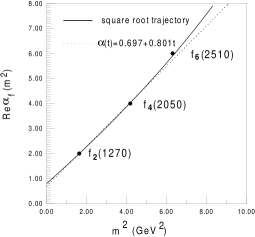
Figure 1: Real part of the $f-$trajectory versus $m^{2}$, squared mass of the resonance. Solid line is the square root trajectory used in the present work (see the text). Dashed straight line is the result of a linear fit.

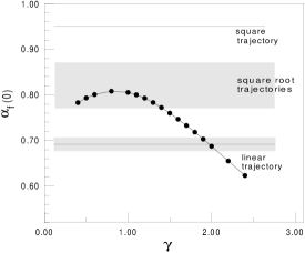
Figure 2: Intercept of the $f-$trajectory correlated with the power $\gamma$ of $\ell ns$ in $\sigma_{tot}(s)$. Intervals for an intercept of various parametrizations are shown.

The following parabola passes exactly through the three known resonances : $\alpha_{f}(t)=\alpha_{f}(0)+\alpha^{\prime}_{f}t+\beta_{f}t^{2}$ with $\alpha_{f}(0)=0.96$, $\alpha^{\prime}_{f}=0.59$ GeV^-2, $\beta_{f}=0.03$ GeV^-4. This leads to a too high intercept and can cause problems in the fit to differential cross-sections at large $|t|$. A more realistic trajectory such as $\alpha_{f}(t)=\alpha_{f}(0)+\gamma_{1}(\sqrt{4m_{\pi}^{2}}-\sqrt{4m_{\pi}^{2}-t}\ )+\gamma_{2}(\sqrt{t_{1}}-\sqrt{t_{1}-t}\ ),$ gives $0.77<\alpha_{f}(0)<0.87$.

Generally, there is an evident correlation between the intercept of the $f-$Reggeon and the model for the Pomeron. This is due to the fact that in all known processes, Pomeron and $f-$Reggeon contribute additively. As a rule, a higher $f-$intercept is associated with a slower growth with energy due to Pomeron contribution (as an example see also [16]). In Fig.2, we illustrate this observation and show how $\alpha_{f}(0)$ is correlated with a power of $\ell ns$ in the behaviour of the total cross-section, if the forward scattering amplitudes are parameterized in the form.

$$A^{hh}(s,0)=i\Big{[}C_{1}+C_{2}\ell n^{\gamma}(-is/s_{0})\Big{]}+R(s,0),$$

where the explicit form of secondary Reggeons contribution $R(s,0)$, depends on the nature of interacting hadrons (see [13, 16] for details). In our opinion, a good way to fix the intercepts of $f-$ and $\omega-$Reggeons is after fitting the total cross-sections. Doing so and avoiding an extra number of parameters, we choose the following form of $f-$trajectory

$$\alpha_{f}(t)=\alpha_{f}(0)+\gamma_{f}(\sqrt{t_{f}}-\sqrt{t_{f}-t})\ ,$$

where the intercept $\alpha_{f}(0)=0.810$ is fixed from the fit [2] to the total cross-sections, the effective threshold $t_{f}=14.964$ GeV² and the parameter $\gamma_{f}=5.504$ GeV^-1 are determined from the fit to the positions of the three known resonances. For $\omega-$trajectory (with only two known resonances and absence of information on possible higher resonances) we use a linear form

$$\alpha_{\omega}(t)=\alpha_{\omega}(0)+\alpha^{\prime}_{\omega}t\ ,$$

with the intercept $\alpha_{\omega}(0)=0.422$ from [2] and with the slope $\alpha^{\prime}_{\omega}=0.946$ GeV^-2 determined in a fit to resonances.

3 The modified additive quark model at $t\neq 0$

The amplitudes under interest are written

$$A^{\bar{p}p}_{pp}(s,t)=A_{\cal P}(s,t)+A_{f}(s,t)\pm\Big{[}A_{\cal O}(s,t)+A_{\omega}(s,t)\Big{]}\ .$$ (7)

The normalization is

$$\sigma_{tot}(s)=8\pi\Im mA(s,t=0),\qquad\frac{d\sigma}{dt}(s,t)=4\pi\left|A(s,t)\right|^{2}\ .$$ (8)

The starting points for a parameterization of all terms in (7) at $t\neq 0$ are the corresponding partial amplitudes defined at $t=0$ in [2] and rewritten in detail in (1-6). A special discussion will be devoted to the Odderon amplitude $a_{\cal O}(s,t)$ which is out of he game at $t=0$. Let us recall that, in accordance with the main assumption of additive quark model (as well as of MAQM [2]), there is an interaction of two (in fact of $3\times 3$) constituent quarks (or lines in terms of diagram), each of them carrying only a part of the momentum $\vec{p}$. Therefore we must define $s_{q}=(p_{1}+p_{2})^{2}=s/9$, for protons assuming that the whole momentum is distributed equally between all quarks in each of them. As concerns the $t$ channel, we consider for Pomeron and $f-$Reggeon a single exchange (one line in $t$ channel in terms of diagram); our Odderon also is supposed to behave as a one Reggeon-exchange. Consequently, we have no reason to divide $t$ in the final amplitude by any number .

3.1 Pomeron

Starting from (1), the Pomeron contribution at $t\neq 0$ will have the form

$$A_{\cal P}(s,t)=9\Big{[}A_{\cal P}^{(1)}(s/9,t)+2A_{\cal P}^{(2)}(2s/9,t)+A_{\cal P}^{(3)}(4s/9,t)\Big{]}\ .$$ (9)

The most direct generalization of $A^{(i=1-3)}_{\cal P}(s,0)$ (in (2)) is to consider all ”coupling constants” $g_{1},g_{2},\zeta_{\cal P}$ as functions of $t$ and to multiply each $A^{i}_{\cal P}(s,0)$ by the usual Regge factor $\Bigl{(}-is/s_{0}\Bigr{)}^{\alpha_{\cal P}(t)-1}$. Namely, we write

$$\begin{array}[]{lll}A^{(1)}_{\cal P}(s,t)=&ig_{1}^{2}(t)\Big{[}-\zeta_{\cal P}(t)+L(s)\Big{]}\Bigl{(}-is/s_{0}\Bigr{)}^{\alpha_{\cal P}(t)-1}\ ,\\ A^{(2)}_{\cal P}(s,t)=&ig_{1}(t)g_{2}(t)\Big{[}-\zeta_{\cal P}(t)+L(s)\Big{]}\Bigl{(}-is/s_{0}\Bigr{)}^{\alpha_{\cal P}(t)-1}\ ,\\ A^{(3)}_{\cal P}(s,t)=&ig_{2}^{2}(t)\Big{[}-\zeta_{\cal P}(t)+L(s)\Big{]}\Bigl{(}-is/s_{0}\Bigr{)}^{\alpha_{\cal P}(t)-1}\ .\end{array}$$ (10)

As the simplest variant we choose the linear Pomeron trajectory (again with an intercept equal 1)

$$\alpha_{P}(t)=1+\alpha^{\prime}_{P}t\ ;$$ (11)

we considere also the case of a logarithmic trajectory which is discussed in details in Section 4. Of course, more sophisticated Pomeron models can be proposed but they lead to an extra number of parameters and we will not consider them. Finally, to avoid proliferation of parameters, we will assume simple exponential ”residue functions” $g_{i=1,2}$ and $\zeta_{\cal P}$

$$g_{1}(t)=g_{1}\exp(b_{1}t),\qquad g_{2}(t)=g_{2}\exp(b_{2}t),\qquad\zeta_{\cal P}(t)=\zeta_{\cal P}\exp(b_{\zeta_{\cal P}}t).$$ (12)

Thus there are seven ($g_{1},g_{2},\zeta_{\cal P},b_{1},b_{2},b_{\zeta_{\cal P}},$ $\alpha^{\prime}_{\cal P}$) parameters for the Pomeron term of amplitude. With this Pomeron model the Froissart-Martin bound is not violated and the total cross-section behaves as $\ell ns$ when $s\to\infty$.

3.2 Secondary Reggeons

Generalizing [2], the $f-$Reggeon amplitude in the MAQM is written as

$$A_{f}(s,t)=(5+4\lambda_{f})A_{f}^{(qq)}(s/9,t)\ ,$$ (13)

where

$$A_{f}^{(qq)}(s,t)=ig_{f}^{2}\Bigl{(}-i\frac{s}{s_{0}}\Bigr{)}^{\alpha_{f}(t)-1}e^{b_{f}t},\quad\alpha_{f}(t)=\alpha_{f}(0)+\gamma_{f}(\sqrt{t_{f}}-\sqrt{t_{f}-t}).$$ (14)

As already noted above, for that $f-$Reggeon trajectory we choose a square-root dependence on $t$, which is more suitable than a linear one, and fix its parameters from the fits to cross-sections and resonances (see Subsection 2.2). The value of $\lambda_{f}$ is unimportant if only $pp$ and $\bar{p}p$ processes are considered (it is equivalent to redefine the coupling $g_{f}$). Nevertheless, for the present work we keep $\lambda_{f}=0.439$ which was obtained from the fit at $t=0$ (see [2]). The number of free parameters for a fixed trajectory is then only two ($g_{f},b_{f}$). Following the previous considerations, we write for the $\omega$-Reggeon

$$A_{\omega}(s,t)=(5+4\lambda_{\omega})A_{\omega}^{(qq)}(s/9,t)\ ,$$ (15)

where

$$A_{\omega}^{(qq)}(s,t)=g_{\omega}^{2}\ \Bigl{(}-i\frac{s}{s_{0}}\Bigr{)}^{\alpha_{\omega}(t)-1}e^{b_{\omega}t},\quad\alpha_{\omega}(t)=\alpha_{\omega}(0)+\alpha^{\prime}_{\omega}t\ .$$ (16)

For the $\omega-$Reggeon trajectory, we recall that we choose a linear dependence on $t$, with the parameters given in Subsection 2.2. In  [12] a multiplicative factor $r_{\omega}(s,t)$ was introduced in $A_{\omega}^{(qq)}(s,t)$ to describe a so called ”cross-over phenomenon”, namely, a zero at small $t$ in the difference of the $\bar{p}p$ and $pp$ differential cross-sections. Here, we extend the kinematic region under consideration up to $|t|\approx 14$ GeV² and also include Odderon contributions. An interference of various odd terms in amplitude could produce now the mentioned zero automatically and thus we set $r_{\omega}(s,t)=1$. Again, repeating the arguments given above for the $f-$Reggeon, we put $\lambda_{\omega}=1.$ When the trajectory is fixed, we are left with only two free parameters ($g_{\omega},b_{\omega}$).

3.3 Odderon

This crossing-odd contribution (added to the $\omega-$Reggeon ) is a quite delicate and ambiguous point, lacking sufficiently precise and numerous data. A widespread consensus [13, 14, 16], however, is that an Odderon contribution while insignificant at $t=0$ is very relevant in the large $|t|$ domain.

As compared with the previous contributions, it is important to notice that it is impossible to apply to the Odderon any additive quark model rule. Odderon, in contrast with Pomeron and secondary Reggeons, interacts with the whole proton rather than with separate quarks since three gluons (or the Odderon by Donnachie and Landshoff [20]) couple simultaneously with three quarks in each $p$ or $\bar{p}$.

As repeatedly mentioned, in this paper we stick to the Born approximation and rescattering corrections are not taken into account. This is known to be inadequate from the conceptual point of view and not just for practical reasons of restoring unitarity when the Born approximation yields its violation. The point is particularly delicate concerning the Odderon which, by universal consensus, should be important at large $|t|$. For this reason, we parameterize the Odderon, somewhat artificially, as the sum of two contributions which we denote as ”soft” and ”hard”

$$A_{\cal O}(s,t)=A_{\cal O}^{(s)}(s,t)+A_{\cal O}^{(h)}(s,t)\ .$$ (17)

As it is known, the contribution of Odderon at $t=0$ is negligible. We take into account this fact multiplying both components by a factor vanishing at $t=0$. For the soft Odderon we assume like for the Pomeron a dipole form, suitably damped 

$$A_{\cal O}^{(s)}(s,t)=g_{{\cal O}s}(t)\Bigl{[}(1-e^{\beta_{s}t})\ell n(-is/s_{0})\Bigr{]}^{\mu}\Bigl{[}-\zeta_{{\cal O}s}(t)+\ell n(-is/s_{0})\Bigr{]}\bigg{(}-i\frac{s}{s_{0}}\bigg{)}^{\alpha_{\cal O}(t)-1},$$ (18)

while for the hard one, we choose

$$A_{\cal O}^{(h)}(s,t)=g_{{\cal O}h}(1-e^{\beta_{h}t})[\ell n(-is/s_{0})]^{\nu}\frac{1}{(1-t/t_{{\cal O}h})^{4}}\ .$$ (19)

We should give here a few comments concerning the choice of the Odderon amplitude defined by the above equations.

1) The contribution of the soft Odderon to $\sigma_{elastic}$ is dominated by the region where $|t|$ is small. In this domain the factor $(1-e^{\beta_{s}t})\ell n(-is/s_{0})$ is nearly constant. It means that the soft Odderon does not violate the evident inequality $\sigma_{elastic}\leq\sigma_{tot}$ at any value of $\mu$.

2) At the same time the amplitude should not have a singularity at $t=0$, therefore $\mu$ must be an integer. In the fits we have considered $\mu=1$ and $\mu=2$.

3) The hard Odderon does not exponentially decrease with $|t|$, therefore it does not violate the restriction $\sigma_{elastic}\leq\sigma_{tot}$ at any $s$ only if $\nu\leq 1/2$.

4) We consider a linear Odderon trajectory but with a non unit intercept, only constrained by unitarity 

$$\alpha_{\cal O}(t)=1+\delta_{\cal O}+\alpha^{\prime}_{\cal O}t\ ,\qquad\delta_{\cal O}\leq 0\ .$$ (20)

In fact, as it will be emphasized below, only the upper bound of the intercept may be kept. 5) As for the Pomeron, the soft residue functions are taken in an ordinary exponential form

$$g_{{\cal O}s}(t)=g_{{\cal O}s}e^{{b_{\cal O}}t},\qquad\zeta_{{\cal O}s}(t)=\zeta_{{\cal O}}e^{b_{\zeta_{\cal O}}t}\ .$$ (21)

The case of a logarithmic trajectory is reserved for discussion. Thus the Odderon contribution is controlled by a maximum of ten additional parameters : $g_{{\cal O}s},\zeta_{\cal O},\beta_{s},$ $b_{\cal O},b_{\zeta_{\cal O}},\delta_{\cal O},\alpha^{\prime}_{\cal O}$, $g_{{\cal O}h},t_{{\cal O}h},\beta_{h}$.

The grand total number of free parameters for MAQM is twenty six, however, this number will be reduced by fixing some of them by virtue of special arguments. For example, this paper being devoted to $pp$ and $\bar{p}p$ angular distributions, all coupling constants and intercepts are fixed from the fit to $\sigma_{tot}$ and $\rho$ at $t=0$ as reported in [2]; furthermore, the remaining parameters of Reggeons trajectories are fixed here from the resonances; not excluding simplifications in the chosen form for the Odderon.

4 Results and discussion

4.1 Previous results at $t=0$ [2]

It is our choice to extract from [2], the useful information concerning $pp$ and $\bar{p}p$ at $t=0$. Of course, we do not claim that better fits are not possible for forward scattering ; many very good ancient and recent parametrizations, that it is not our scope to discuss here, are available for $pp$ and $\bar{p}p$ processes. Thus, as a first step, we refer to the results found in [2], where 217 $t=0$ data (for $pp$ and $\bar{p}p$) with 4 GeV$\leq\sqrt{s}\leq$1800. GeV ([21]) have been taken into account, within combined fits of $pp,\,\bar{p}p,\,\pi^{-}p,\,\pi^{+}p,\,\gamma\gamma,\,\gamma p$ total cross-sections and $\rho-$ ratios. The selected results under interest here are given in the Table 1 which exhibits the improvement brought to the old AQM by the modifications called in the revisited AQM.

Observable	$\sigma^{pp}_{tot}$	$\sigma^{\bar{p}p}_{tot}$	$\rho^{pp}$	$\rho^{\bar{p}p}$
Number of points	85	51	64	17
$\chi^{2}$ SAQM	220	240	157	17
$\chi^{2}$ MAQM	53	59	147	18

Table 1. The partial $\chi^{2}$-s obtained by fitting at $t=0$ [2] in the SAQM (old) and the MAQM (modified).

The $\chi^{2}/d.o.f.$ (for the all processes) was 1.78 in the MAQM (remind that we fitted our model to the data at $\sqrt{s}\geq 4$ GeV instead of $\sqrt{s}\geq 5$ GeV in [13, 16]). The recalculated $\chi^{2}/d.o.f.$ (specifically for $pp$, $\bar{p}p$ processes) is 1.32 in the MAQM. The corresponding behavior of $\sigma_{tot}(s)$ and of $\rho(s)=\Re eA(s,0)/\Im mA(s,0)$ are plotted in [2]. To complete, we give in Table 2 the parameters issued from the combined fits in [2], used here for the $pp$ and $\bar{p}p$ processes.

Parameter	$g_{1}$(GeV-1)	$g_{2}$(GeV-1)	$\zeta_{P}$	$g_{f}$(GeV-1)	$\alpha_{f}(0)$	$g_{\omega}$(GeV-1)	$\alpha_{\omega}(0)$
Value in
MAQM	0.3166	$-$ 0.0239	3.396	1.112	0.8100	0.3948	0.4217

Table 2. Values of the parameters controlling the MAQM amplitudes at $t=0$ [2]. Recall the Pomeron intercept equals 1. and the values quoted for $g_{f}$ and $g_{\omega}$ are coupled to $\lambda_{f}=0.439$ and $\lambda_{\omega}=1.$ respectively.

4.2 MAQM results at $t\neq 0$

The previous seven parameters are kept fixed to their values determined by the $t=0$ combined fits. In addition, we fixed from fits to the resonances those parameters of the Reggeon trajectories relevant at $t\neq 0$. Their determination in the present work are recalled in Table 3 (see also Subsection 2.2).

Reggeon	”f”		”$\omega$”
trajectory	square-root (14)		linear (16)
number of data	3 resonances		2 resonances
parameter	$\gamma_{f}$	$t_{f}$	$\alpha^{\prime}_{\omega}$
	5.504 GeV-1	14.964 GeV2	0.9459 GeV-2

Table 3. Values of the parameters driving the Reggeon trajectories at $t\neq 0$, determined by fitting the resonances.

Only the remaining parameters are fitted in isolation from the angular distributions. Of course, the final $\chi^{2}$ could be improved by refitting the complete set of parameters for the $pp$ and $\bar{p}p$ processes alone but we decide against doing so. In this second step, we account for 959 $t\neq 0$ data [21] with 0.1$<|t|$(GeV²)$\leq 14.2$; 19.4$\leq\sqrt{s}$(GeV)$\leq$630. The selection $|t|>0.1$ GeV² is used in order to exclude the Coulomb-nuclear interference region. It could be included as a refinement. After preliminary trials, we select the following conditions for the current parameterization : (i) $\mu=2$ is chosen here because it gives a slightly better $\chi^{2}$, but, taking $\mu=1$ does not influence significantly the quality of the fit: once more the data do not seem precise enough to select a specific form of the Odderon

(ii) $\nu=1/2$: for this (maximal) value, the Odderon does not violate unitarity, the results at high energy (LHC) do not seem abnormal and the Odderon can be considered as an effective phenomenological contribution

(iii) one may fix without damaging the results a unit intercept for the Odderon ($\delta_{\cal O}=0$) as for our Pomeron and in agreement with [22] (iv) linear trajectories are used throughout (except for the $f$), which represents the more economic (if not the more efficient) solution

(v) furthermore, as unitarity requires [23], we constrained $\alpha^{\prime}_{od}\leq\alpha^{\prime}_{p}$.

We found the results distributed according to Table 4.

Observable	$({d\sigma/dt})^{pp}$	$({d\sigma/dt})^{\bar{p}p}$
Number of points	758	201
$\chi^{2}$	1636	616

Table 4. Resulting partial $\chi^{2}$-s obtained by fitting the angular distributions in the MAQM with the parameters in Table 5.

The corresponding $\chi^{2}/d.o.f.$ (for $t\neq 0$) is 2.38 (for 959 data and 15 parameters listed in Table 5) and recalculated with the $t=0$ and $t\neq 0$ data together (with the couplings and intercepts given in Table 2) is 2.19 (for 1176 data and 22 parameters).

Pomeron	$b_{1}$,  GeV-2	.1975E+01
	$b_{2}$,  GeV-2	$-$.2121E+00
	$b_{\zeta_{\cal P}}$, GeV-2	.1227E+01
	$\alpha^{\prime}_{\cal P}$,  GeV-2	.3308E+00
$f-$Reggeon	$b_{f}$,  GeV-2	.4094E+01
$\omega-$Reggeon	$b_{\omega}$, GeV-2	$\approx$ 0.0
Odderon	$g_{{\cal O}s}$,  GeV-2	$-$.1305E$-$02
(soft)	$\zeta_{\cal O}$	.2234E+02
	$\beta_{s}$,  GeV-2	.5023E+01
	$b_{\cal O}$,  GeV-2	$-$.1693E+00
	$b_{\zeta_{\cal O}}$, GeV-2	.1417E+01
	$\alpha^{\prime}_{\cal O}$,  GeV-2	.3208E+00
Odderon	$g_{{\cal O}h}$,  GeV-2	.2434E+01
(hard)	$t_{{\cal O}h}$,  GeV2	.4137E+00
	$\beta_{h}$,  GeV-2	.1197E+01

Table 5. Parameters of MAQM obtained in fitting the angular distributions.

We found, within the MAQM, a pretty good reproduction of the data (including the dip and the high $|t|$ regions), exhibited in Figs. 3-4.

Figure 3: Fit of the differential cross-sections of $pp$ interaction, calculated in MAQM. A factor 10^-2 between each successive energy is omitted.

Figure 4: The same as in Fig. 3, for $\bar{p}p$. The Tevatron data are not fitted.

Searching for an improvement of our results (and accepting to ”measure” the quality of a model by the $\chi^{2}/d.o.f.$ because we have nothing better), as already said, it is possible to get a better agreement with the data when refitting all the parameters together to the forward and non forward observables, for $pp$ and $\bar{p}p$ only. In that case, we find only a non significant improvement in the sense that no modifications is seen on the figures. Any significant improvement of the $\chi^{2}$ is not automatically followed by an improvement visible on the curves. It is of some interest to compare our results with those of other approaches. A strict comparison is not easy because, if many of them are available, they present different objectives, and it is not our aim to discuss the relative virtues and shortcomings of each work. The model of [8] for example is an eikonalized model, not operating at the Born level like ours, in which the energy dependence of the amplitude is absorbed in the parameters. At the Born level, the nearest models are probably the old models of [20, 6], based on the Regge theory, furthermore their results are grossly comparable to ours. The first one contains in particular a two-Pomeron exchange and other cuts contributions which are absent in our approach. The second one involves a large number of parameters and the data at high $|t|$ are not correctly reproduced.

4.3 Unitarity, Odderon and logarithmic trajectories.

-1) As a by-product of the present study, we propose to consider the scattering amplitude obtained in our MAQM from the point of view of unitarity and analyticity. To be specific we want to insure that this amplitude not only respects the Froissart-Martin bound but also exhibits a zero at low $|t|$ in $\Re eA^{+}(s,t)$, real part of its even contribution (with respect to the C-parity), as required by a high energy theorem recently stated by A. Martin [17].

The situation of the first zero of $\Re eA^{+}(s,t)$ is shown in Table 6 for some selected high energies. We agree with the theorem, with the results quoted in [17] and some of the extensive discussion [8] exhibiting in particular a first zero of the real part at low $|t|$, decreasing monotonically with the energy. By also reporting $\Re eA_{\cal P}(s,t)$ in Table 6, we exhibit a manifestation of the dominance of the Pomeron at high energies, when the $f-$Reggeon contribution becomes negligible above the ISR energy range.

Energy	zero of $\Re eA^{+}$	zero of $\Re eA_{\cal P}$
(GeV)	$-t$ (GeV2)	$-t$ (GeV2)
546	0.31	0.37
1800	0.27	0.29
10000	0.21	0.22
14000	0.21	0.22

Table 6. First values of $-t$ cancelling $\Re eA^{+}(s,t)$ and $\Re eA_{\cal P}(s,t)$, versus the energy, obtained in the MAQM fit.

-2) $\Im mA^{+}(s,t)$, imaginary part of the even component of the amplitude, has an oscillatory behavior for large $|t|$, in spite of lacking any rescatterings corrections in the model. This is a consequence of the negative sign of the new MAQM (comparing with the old SAQM) coupling constant $g_{2}$ (see Table 2). Oscillations, or something appearing as diffraction-like secondary structures are hidden in the differential cross-sections because of the Odderon contribution dominating in this domain. Of course our present MAQM model cannot produce any oscillations at large $|t|$, because it is a model at the Born approximation level, in which the Odderon dominates at very high energy and in the high $|t|-$region with the behavior in $\sim 1/t^{4}$ of the amplitude (see (19)). As a next step, it would be interesting to eikonalize the model to see in particular if oscillations in $d\sigma/dt$ appear. We believe that rescattering corrections (we plan to calculate them in a near future) may be important at such high energies to be investigated for instance in the TOTEM and PP2PP projects (see for example [24]) and as a consequence any extrapolation (in particular those of the angular distributions) may be doubtful within the present version of non-eikonalized MAQM model.

-3) As already mentioned above, the ”hard” component of the Odderon with a power behaviour at large $|t|$ looks affectedly from the point of view of Regge approach (note here that for the whole set of data, the ratio $|t|/s$ is small, we are in a domain of small angle scattering, that, we believe, should be described by Regge theory while the hard Odderon component can be important at larger $|t|$).

Taking into account the above argument we have considered the model without its ”hard” Odderon component, but for Pomeron and (soft) Odderon we have tested the nonlinear trajectories with a logarithmic behavior

$$\alpha_{i}(t)=1+\gamma_{i}\Big{[}1-(1-t_{i}/t)\ell n(1-t/t_{i})\Big{]},\qquad i={\cal P},\ {\cal O}.$$ (22)

The minimal value of the threshold $t_{\cal P}$ (there are many thresholds in $t$-channel for $pp$ and $\bar{p}p$) should be given by the $t$-channel physical state with the minimal mass (in our case a two-pion state, so $t_{\cal P}^{min}=4m_{\pi}^{2}$). Nevertheless, in order to take into account the influence of other thresholds we consider $t_{\cal P}$ as a free (effective) parameter. A similar argument can be repeated for the Odderon trajectory.

Logarithmic trajectories mimic a power decreasing amplitude with $|t|\to\infty$. However, in order to give a sense to such a possibility, it is necessary to replace the exponential residue functions by power ones. It leads to an extra number of free parameters. Therefore we used another, probably oversimplified, method. All exponents, $\exp(b_{i}t)$ in the Pomeron and in the soft Odderon terms are replaced by $\exp[(\alpha_{\cal P(O)}(t)-1)b_{i}]$. Using logarithmic trajectories, we do not aim to obtain the best fit, rather we only want to check our belief (and to demonstrate for a reader) that it is then possible to reproduce large $|t|$ data.

Resulting $\chi^{2}/d.o.f=3.39$ as well as agreement with data is not so bad. The calculated angular distributions are deviated slightly from the data points mainly around the dips for $pp$ but, as we expected, are very well reproduced for the large$-|t|$ domain.

Summarizing, we emphasize that the obtained results confirm and reinforce the conclusion of [2] as a further test of the model: account of the corrections to a Pomeron-quark interaction and new counting rules for the secondary Reggeons. In other words using the modified additive quark model instead of the standard additive quark model, leads to a good agreement with available experimental data not only at $t=0$, but also at $t\neq 0$. Besides we found that data on the elastic $pp$ and $\bar{p}p$ scattering at high energies can be reproduced with a high quality in a model with the Dipole Pomeron, which has a unit intercept, $\alpha_{\cal P}(0)=1$ leading to an intermediate growth of the total cross-sections, $\sigma_{tot}(s)\propto\ell ns$ when $s\to\infty$. Finally, a zero at small $|t|$ reveals in the real part of the even amplitude, in agreement with a high energy theorem by Martin.

Acknowledgements. We are indebted to E. Predazzi for his support and discussions. Two of us (MG and EM) would like to thank the Dipartimento di Fisica Therica of the University of Torino for kind hospitality. EM thanks also the Institut de Physique Nucléaire de Lyon for the hospitality. Financial support by the INFN and the MURST of Italy and from the IN2P3 of France is gratefully acknowledged.

References

-
[1]
E.M. Levin, L.L. Frankfurt, Pisma ZhETP,
3, 105 (1965);
H.J. Lipkin, F. Sheck, Phys. Rev. Lett. 16, 71 (1966);
J.J.J. Kokkedee, L. Van Hove, Nuovo Cim. 42A, 711 (1966) - [2] P. Desgrolard, M. Giffon, E. Martynov, E. Predazzi, Eur. Phys. J. C 9, 623 (1999)
- [3] T.T. Chou, C.N. Yang, Phys. Rev. 170, 1591 (1968); Phys. Rev. Lett. 20, 1213 (1968); Phys. Rev. D 17, 1889 (1978) C. Bourrely, J. Soffer, T.T. Wu, Phys. Rev. D 19, 3249 (1979); Nucl. Phys. B 247, 15 (1984); C. Bourrely, in Elastic and Diffractive Scattering at the Collider and beyond, 1st International Conference on Elastic and Diffractive Scattering, Chateau de Blois, France (1st ”Blois workshop”) - June 1985, edited by B. Nicolescu and J. Tran Thanh Van (Editions Frontières, 1986) p.239 L.L. Jenkovszky, B.V. Struminsky, A.N. Wall, Sov. J. Part. Nucl. 19, 180 (1988)
- [4] P. Desgrolard, M. Giffon, E. Predazzi, Z. Phys. C 63, 241 (1994)
- [5] R.J.M. Covolan, J. Montanha, K. Goulianos, Phys. Lett. B 389, 176 (1996)
- [6] P. Gauron, B. Nicolescu, E. Leader, Nucl. Phys. B 299, 640 (1988); Phys. Lett. B 238, 406 (1990)
- [7] L.L. Jenkovszky, Fortschr. Phys. 34, 702 (1986); M. Bertini et. al., Rivista Nuovo Cim. 19, 1 (1996) and references therein.
- [8] F. Pereira, E. Ferreira, Phys. Rev. D 59, 014008 (1998); ibid. 61, 077507 (2000)
- [9] E. Levin, An introduction to Pomerons, DESY 98-120, TAUP 2522/98, e-Print archive : hep-ph/9808486; E. Predazzi, Diffraction : past, present and future, Lectures given at Hadrons VI, Florianopolis, Brazil - March 1998, DFTT 57/98, e-Print archive : hep-ph/9809454
- [10] P. Desgrolard, M. Giffon, E. Martynov, E. Predazzi, Eur. Phys. J. C 14, 683 (2000)
- [11] M. Giffon, E. Martynov, E. Predazzi, Z. Phys. C 76, 155 (1997); see also [23]
- [12] P. Desgrolard, A. Lengyel, E. Martynov, Nuovo Cim. A 110, 251 (1997)
- [13] P. Desgrolard, M. Giffon, A.I. Lengyel, E. Martynov, Nuovo Cim. A 107, 637 (1994)
- [14] P. Desgrolard, M. Giffon, E. Martynov, Nuovo Cim. A 110, 537 (1997)
- [15] M. Block, K. Kang, A.R. White, Mod. Phys. A 7, 4449 (1992)
- [16] J. R. Cudell et al., Phys. Rev. D 61,034019 (2000)
- [17] A. Martin, Phys. Lett. B 404, 137 (1997)
- [18] P. Desgrolard, A. Lengyel, E. Martynov, Eur. Phys. J. C 7, 655 (1999)
- [19] A. Donnachie, P.V. Landshoff, Phys. Lett. B 387, 637 (1996)
- [20] A. Donnachie, P.V. Landshoff, Z. Phys. C 2, 55 (1977); Nucl. Phys. B 231, 189 (1984); ibid. 244, 322 (1984); ibid. 267, 406 (1986)
- [21] The data used have been extracted from the PPDS, accessible at http://pdg.lbl.gov (computer readable data files).
- [22] J. Bartels, L.N. Lipatov, G.P. Vacca, Phys. Lett. B 477, 178 (2000)
- [23] J. Finkelstein, H.M. Fried , K. Kang, C.-I. Tan, Phys. Lett. B 232, 257 (1989); E. Martynov, Phys. Lett. B 232, 367 (1989); H.M. Fried, in ”Functional Methods and Eikonal Models” (Editions Frontières, 1990) p.214
- [24] S.B. Nurushev, in Proceedings of the International conference on Elastic and Diffractive Scattering, (VIIIth EDS Blois Workshop), Protvino, Russia, 1999, edited by V.A. Petrov and A.V. Prokudin (World Scientific Publishing, 2000) p.313; S. Weisz, Talk at the International conference on Elastic and Diffractive Scattering, (VIIIth EDS Blois Workshop), Protvino, Russia (june 26-july 2, 1999).