Leontovich Relations in Thermal Field Theory

Abstract

The application of generalized Kramers-Kronig relations, the so-called Leontovich relations, to thermal field theory is discussed. Medium effects contained in the full, thermal propagators can easily be taken into account by this method. As examples the collisional energy loss of a charged particle in a relativistic plasma and the radiation of energetic photons from a quark-gluon plasma are considered. Within the leading logarithmic approximation the results based on the hard thermal loop resummation technique are reproduced easily. However, the method presented here is more general and provides exact expressions, which allow in principle non-perturbative calculations.

I Introduction

Naively one expects that high energy particles, weakly interacting with a medium, can be treated perturbatively. The basic process (production, absorption, or scattering) should follow from lowest order perturbation theory as in vacuum. The only role of the medium is to provide the particles with which the high energy particle interacts. In other words, medium effects enter the cross section only via the distribution functions of the in-medium particles. Note, however, that in the case of bosons the cross sections can be infrared enhanced due to Bose condensation. Famous examples are the effective medium dependent masses of neutrinos interacting with the solar or terrestrial matter leading to medium induced neutrino oscillations. These masses follow directly from integrating over the electron distribution [1]. Note that it is not even necessary that these distributions are in equilibrium. Another example is the production of dileptons with high invariant masses from a quark-gluon plasma (QGP), which is given to lowest order by the annihilation of bare quarks and anti-quarks (Born term) [2]. Due to phase space the main contribution comes from quarks in the high energy tail of the distributions. At lower invariant masses ($M<1$ GeV) bare quarks are not sufficient and additional medium effects will lead to interesting structures in the dilepton production rate [3].

The quantities mentioned above, namely the effective neutrino mass and the dilepton production, are infrared finite to lowest order perturbation theory. In some cases, however, the lowest order contribution suffers from infrared divergences. In this case additional medium effects even for high energy, weakly interacting particles are essential. If the quantity under consideration has a logarithmic infrared singularity within naive perturbation theory, a finite result can be obtained by using hard thermal loop (HTL) resummed propagators for soft momentum transfers [4]. However, some quantities, e.g. damping rates [5], which exhibit a higher infrared singularity, cannot be calculated to leading order using the HTL method. Also contributions beyond the leading logarithm might require a non-perturbative treatment [6].

Here we will demonstrate, considering two examples, that the leading logarithmic contributions can be calculated easily using generalized Kramers-Kronig relations. In contrast to the HTL improved perturbation theory the knowledge of the resummed propagator is required only in the high frequency limit. The method presented here is much more general as exact expressions can be derived, which allow in principle non-perturbative results, if only the full propagator in the high frequency limit is known.

In the next section we discuss the usefulness of the Leontovich relation for thermal field theoretic calculations in the case of the collisional energy loss of charged particles in a relativistic plasma. This quantity has already been considered by Kirzhnits [7] using the Leontovich method within the language of plasma physics and recently by the author within thermal field theory [8]. Therefore we will discuss this quantity only briefly focusing on the use of the Leontovich relation. In section 3 we show in more detail that the production rate of high energy photons from a quark QGP can be treated in a similar way. For this purpose we generalize the Leontovich relation used so far only for gauge bosons to quarks.

II Collisional Energy Loss

The energy loss of a fast charged particle in a medium is a well studied subject [9]. Recently the energy loss of energetic particles, such as leptons and partons, in relativistic plasmas has attracted great interest. In relativistic heavy ion collisions the energy loss of a high energy quark or gluon coming from primary hard collisions in the fireball will lead to jet quenching. Jets therefore serve as a direct probe for the fireball and may provide a signature for the quark-gluon plasma formation [10]. In Supernovae explosions the energy loss of neutrinos, having a weak charge, in the plasma surrounding the stellar core might be an important mechanism for triggering the explosion [11].

The total energy loss of a particle in a medium can be decomposed into a collisional and a radiative contribution. While the first one originates from the energy transfer to the medium particles, the latter one is caused by radiation from the fast particle. Here we want to consider only the collisional component.

The collisional energy loss is defined as the energy transferred per unit length from the fast particle to the medium in a single collision. It is assumed that the fast particle loses only a small fraction of its energy in each collision. In quantum field theory the collisional energy loss is defined as [12]

$$\frac{dE}{dx}=\frac{1}{v}\>\int d\Gamma\>\omega,$$ (1)

where $v$ is the velocity of the incident particle with energy $E$ and $\omega=E-E^{\prime}$ the energy transfer to the medium. The interaction rate $\Gamma$ is identical with the inverse mean free path. It can be calculated either from the matrix element of the process responsible for the energy loss or equivalently from the imaginary part of the self energy $\Sigma$ of the particle with four momentum $P=(E,{\bf p})$, and mass $M$, ($p=|{\bf p}|$) [12]

$$\Gamma(E)=-\frac{1}{2E}\>[1-n_{F}(E)]\>tr[(P\!\!\!\!/\,+M)\,Im\,\Sigma(E,p)],$$ (2)

where $n_{F}(E)=1/[\exp(E/T)+1]$ is the Fermi distribution in the case of a fermion propagating through a plasma of temperature $T$. In the following we restrict ourselves to electrons or muons with high energies $E\gg T$ in an electron-positron plasma.

To lowest order the interaction rate is caused by elastic scattering of the fast lepton off the thermal electrons and positrons via one-photon exchange. Due to the massless photon this rate is quadratically infrared divergent in naive perturbation theory and cannot be regulated using a HTL photon propagator containing Debye screening. The collisional energy loss, on the other hand, due to the additional factor $\omega$ in the integrand of (1) is only logarithmically infrared divergent within naive perturbation theory and finite within the HTL improved perturbation theory. Such a quantity can be calculated by introducing a separation scale $eT\ll k^{*}\ll T$ for the momentum transfer [4]. Restricting to the leading logarithmic approximation it is sufficient to consider the soft momentum transfer $k<k^{*}$ only. Since the final result must be independent of $k^{*}$, it follows from the soft contribution simply by replacing $k^{*}$ by the maximum momentum transfer. In the soft part of the energy loss a dressed propagator, containing medium effects such as Debye screening, has to be used to regulate the infrared singularity. The exchange of a soft collective photon or plasma mode corresponds to the energy loss by polarization of the medium, also known as Fermi density effect [9].

The collisional energy loss, caused by the exchange of a single dressed photon, follows from a one-loop approximation for $\Sigma$. Here we allow for the most general photon propagator, indicated by the blob in Fig.1. Then we find for ultrarelativistic electrons or muons ($v=1$) [12]

$$\left({\frac{dE}{dx}}\right)_{soft}=\frac{e^{2}}{4\pi}\>\int_{0}^{k^{*}}dk\>k\>\int_{-k}^{k}d\omega\>\omega\>\left[\rho_{l}(\omega,k)+\left(1-\frac{\omega^{2}}{k^{2}}\right)\rho_{t}(\omega,k)\right],$$ (3)

where $\rho_{l,t}$ are the spectral functions of the full photon propagator, defined as

$$\rho_{l,t}(\omega,k)=-\frac{1}{\pi}\>Im\,D_{l,t}(\omega,k).$$ (4)

The full photon propagator fulfills the Kramers-Kronig relation

$$D_{l,t}(k_{0},k)=\int_{-\infty}^{\infty}d\omega\>\frac{\rho_{l,t}(\omega,k)}{k_{0}-\omega+i\varepsilon}.$$ (5)

At finite temperature the photon propagator has only two independent components, given in Coulomb gauge by the longitudinal and transverse propagators [13]

$$D_{l}(k_{0},k) = \frac{1}{k^{2}-\Pi_{l}(k_{0},k)+i\varepsilon},$$ (6)

$$D_{t}(k_{0},k) = \frac{1}{k_{0}^{2}-k^{2}-\Pi_{t}(k_{0},k)+i\varepsilon},$$ (7)

where $\Pi_{l,t}$ are the longitudinal and transverse components of the polarization tensor. It should be noted that the soft collisional energy loss, discussed here, follows according to (3) only from the exchange of one dressed space-like ($\omega^{2}-k^{2}<0$) photon from the particle to the medium. However, the medium particles may undergo further interactions. The physical process corresponding to the imaginary part of the self energy of Fig.1 can be found by using cutting rules. An example is shown in Fig.2. There is no diagram, where to or more photons are emitted from the fast particle, as in the case of the radiative energy loss.

Now we introduce the photon response function

$$R(k_{0},k)=-k^{2}\>D_{l}(k_{0},k)+(k_{0}^{2}-k^{2})\>D_{t}(k_{0},k).$$ (8)

Making the substitution $k\rightarrow q=\sqrt{k^{2}-\omega^{2}}$, i.e. introducing the magnitude of the four momentum of the exchanged photon, and using $Im\,R(-\omega)=-Im\,R(\omega)$, which follows from the general property $\rho_{l,t}(-\omega)=-\rho_{l,t}(\omega)$ [14], we find

$$\left({\frac{dE}{dx}}\right)_{soft}=\frac{e^{2}}{2\pi^{2}}\>\int_{0}^{q^{*}}dq\>q\>\int_{0}^{\infty}d\omega\>\omega\>\frac{Im\,R(\omega,\sqrt{q^{2}+\omega^{2}})}{q^{2}+\omega^{2}}$$ (9)

with $q^{*}\ll T$. Eq. (9) agrees with Ref.[7], which is based on plasma physics arguments if we replace there $Q^{2}$ by $e^{2}/4\pi$.

The response function $R$ fulfills the following Kramers-Kronig relation [7]

$$R(k_{0},k)=\tilde{R}+\frac{2}{\pi}\>\int_{0}^{\infty}d\omega\>\omega\>\frac{Im\,R(\omega,k)}{\omega^{2}-k_{0}^{2}-i\varepsilon},$$ (10)

which can be shown to be equivalent to (4), if we use $\rho_{l,t}(-\omega)=-\rho_{l,t}(\omega)$. Here $\tilde{R}=\lim_{k_{0}\rightarrow\infty}Re\,R(k_{0},k)$.

The Kramers-Kronig relation (10) can be generalized by making a Lorentz transformation from $\omega$ and ${\bf k}$ to $\omega^{\prime}$ and ${\bf k^{\prime}}$ given in a system which moves with the velocity ${\bf u}$ relative to the initial system. Following the arguments in Ref.[15, 16], choosing ${\bf u}\cdot{\bf k}=0$ and $|{\bf u}|=1$, and utilizing that $R(\omega,{\bf k})$ depends only on $k$ in an isotropic and homogeneous medium we obtain the Leontovich relation [7]

$$R(k_{0},\sqrt{k^{2}+k_{0}^{2}})=R_{\infty}+\frac{2}{\pi}\>\int_{0}^{\infty}d\omega\>\omega\>\frac{Im\,R(\omega,\sqrt{k^{2}+\omega^{2}})}{\omega^{2}-k_{0}^{2}-i\varepsilon},$$ (11)

where $R_{\infty}=\lim_{k_{0}\rightarrow\infty}Re\,R(k_{0},\sqrt{k^{2}+k_{0}^{2}})$.

The $\omega$-integral

$$I=\frac{2}{\pi}\>\int_{0}^{\infty}d\omega\>\omega\>\frac{Im\,R(\omega,\sqrt{q^{2}+\omega^{2}})}{q^{2}+\omega^{2}}$$ (12)

appearing in the energy loss (9) agrees with the integral on the right hand side of the Leontovich relation, if we replace $k_{0}$ by $iq$ and $\sqrt{k^{2}+k_{0}^{2}}$ by 0, i.e. $k^{2}=q^{2}$, in (11). Therefore we can write [7]

$$I=R(iq,0)-R_{\infty}.$$ (13)

The zero momentum limit of the response function vanishes due to the fact that there is no preferred direction in the medium at vanishing momentum [7]. Consequently, all we have to know is the response function in the high frequency limit $R_{\infty}$ to find the collisional energy loss in the leading logarithmic approximation. Defining

$$\omega_{0}^{2}\equiv\lim_{k_{0}\rightarrow\infty}\Pi_{t}(k_{0},\sqrt{q^{2}+k_{0}^{2}})$$ (14)

we obtain from (8)

$$R_{\infty}=-\frac{\omega_{0}^{2}}{q^{2}+\omega_{0}^{2}}.$$ (15)

Using the Kramers-Kronig relation for the transverse dielectric function, which is related to the transverse polarization tensor [8], Kirzhnits argued [7] that $\omega_{0}$ is independent of $q$ and can be considered as the effective thermal mass of the transverse high frequency plasma excitations, which is given by $\omega_{0}^{2}=e^{2}n\langle 1/\Omega\rangle$ in the relativistic limit. Here $n$ is the number density of the medium and $\Omega$ the energy of the plasma particles.

Combining (15) with (9) and replacing $q^{*}\gg\omega_{0}$ by $q_{max}$, which is proportional to $\sqrt{ET}$ in the relativistic limit $E\gg\Omega$ [7], we end up with the final result for total collisional energy loss

$$\frac{dE}{dx}=\frac{e^{2}}{4\pi}\>\omega_{0}^{2}\ln\frac{q_{max}}{\omega_{0}}.$$ (16)

This result is “exact” in the sense that it is independent of any approximation to the full photon propagator. To logarithmic accuracy the final result just depends on the parameter $\omega_{0}$.

To proceed from here we have to make an approximation for $\omega_{0}$. Since in the high frequency limit medium effects are small, we calculate $\omega_{0}$ by lowest order perturbation theory. Adopting the gauge invariant expression for the transverse polarization tensor in the high temperature limit [17], we obtain $\omega_{0}^{2}=3m_{\gamma}^{2}/2$, where the plasma frequency is given by $m_{\gamma}=eT/3$. As expected $\omega_{0}$ is equivalent to the high frequency mass of the transverse photon $\omega_{0}^{2}=e^{2}n\langle 1/\Omega\rangle$ [8]. Inserting the high temperature result for $\omega_{0}$ in (16) leads to an estimate for the collisional energy loss which agrees to leading logarithm with the one found in the HTL approximation [12]

$${\frac{dE}{dx}}=\frac{e^{2}}{4\pi}\>\omega_{0}^{2}\left(\ln\frac{\sqrt{ET}}{\omega_{0}}+0.120\right).$$ (17)

In contrast to the HTL method we only had to know the transverse polarization tensor in the high frequency limit. Moreover, we observe that the HTL result has already the same form as the exact result (16), which includes infinitely many higher order diagrams such as the one in Fig.2. Assuming that the exact high frequency transverse polarization tensor can be approximated by its high temperature limit we find that the complete collisional energy loss can be estimated by its lowest order HTL result (17) and that higher order diagrams can be neglected at least within the leading logarithm approximation.

In Ref.[8] this result has been applied to the energy loss of energetic partons in a QGP. It has been shown that the radiative energy loss [18] caused by bremsstrahlung from the fast particle, which increases linearly with the distance $L$ over which the parton propagates, dominates over the collisional one for $L>1$ fm.

Another application of (16) has been discussed in Ref.[19] in connection with the neutrino energy loss in matter. Here the collisional energy loss provides a reliable estimate of the total energy loss since bremsstrahlung from the neutrino, i.e. emission of a $Z$ boson, is suppressed by the large mass of the gauge boson at least for temperatures below $T\simeq 100$ GeV.

III High Energy Photons

Now we want to discuss another example, namely the production of high energy real photons in the QGP, which might also serve as a promising signature for the QGP formation in relativistic heavy ion collisions [20]. Due the weak interaction of photons with the QGP photons present as well as jet quenching a direct probe for the hot fireball. To lowest order the production rate of real photons is given by the diagrams of Fig.3 (Compton scattering, annihilation with gluon absorption). Here an intermediate bare quark appears, which can be assumed to be massless as the bare mass of up and down quarks can be neglected compared to the temperature $T$ of the QGP. This leads to a logarithmic infrared divergence in the production rate, which is regulated by medium effects.

The production rate corresponding to the processes of Fig.3 can be calculated by using the HTL resummed quark propagator in the case of a soft quark exchange, i.e. momentum exchange much smaller than $T$. This corresponds to a one-loop calculation including a HTL quark propagator, that contains an effective quark mass of the order $gT$, which cuts off the logarithmic singularity. For the hard momentum transfer the tree level scattering matrix elements convoluted with the parton distribution functions can be used [21, 22, 23]. In this way the production rate of energetic photons to leading logarithmic order $\alpha_{s}\ln(1/\alpha_{s})$ in the strong coupling constant has been obtained.

Here we will derive the photon rate to leading logarithm, using the Leontovich relation for the full quark propagator, which allows a more general and after all simpler derivation of the rate than applying the HTL method. For this purpose we calculate the photon production rate from the imaginary part of the polarization tensor according to [21]

$$E\frac{dR}{d^{3}p}=-\frac{2}{(2\pi)^{3}}\>\frac{1}{e^{E/T}-1}\>Im\,\Pi_{\mu}^{\mu}(E).$$ (18)

This expression is exact to all orders in $\alpha_{s}$ and to leading order in $\alpha$.

Here we focus only on the soft contribution to the photon rate since the hard contribution can be calculated perturbatively from Fig.1 restricting to the logarithmic approximation. Since the energy of the produced photon is high ($E\gg T$) the polarization tensor is given by Fig.4. The blob denotes the full non-perturbative quark propagator. Due to kinematics there is only one full quark propagator, since the other one has to be hard, and no vertex correction since the high energy photon resolves the vertex completely. By cutting this polarization tensor one observes that all processes are taken into account, where the soft quark interacts with the medium in all possible ways. For example it can absorb a thermal gluon as in Fig.3. But also bremsstrahlung from the thermal particles and other higher order processes are included.

Now we want to calculate the photon production rate from Fig.4 for the most general full quark propagator without assuming any approximation for it. For this purpose, we proceed similarly as in the case of the collisional energy loss for energetic charged particles in a plasma. We start from an exact expression for the imaginary part of the soft polarization tensor in the case of two massless quark flavors using $E\gg T$ [21]

$$Im\,\Pi_{\mu}^{\mu}(E)=\frac{5e^{2}}{12\pi}\>\int_{0}^{\infty}dk\int_{-k}^{k}d\omega\>[(k-\omega)\rho_{+}(\omega,k)+(k+\omega)\rho_{-}(\omega,k)]\>\theta(q_{c}^{2}-k^{2}+\omega^{2}),$$ (19)

where $q_{c}\ll T$ is the separation scale between the soft and the hard contribution, $\omega$ and $k$ the energy and the magnitude of the three momentum of the soft quark, and $\rho_{\pm}$ the spectral functions of the full quark propagator $S(K)$ in the helicity representation [24]

$$\rho_{\pm}(\omega,k)=-\frac{1}{\pi}\>Im\,\frac{1}{D_{\pm}(\omega,k)}$$ (20)

with ($K=(k_{0},{\bf k})$)

$$S(K)=\frac{\gamma_{0}-{\bf\hat{k}}\cdot\mbox{\boldmath$\gamma$}}{2D_{+}(k_{0},k)}+\frac{\gamma_{0}+{\bf\hat{k}}\cdot\mbox{\boldmath$\gamma$}}{2D_{-}(k_{0},k)}.$$ (21)

Replacing again $k$ by $q=\sqrt{k^{2}-\omega^{2}}$ in the integral of (19) we find

$$Im\,\Pi_{\mu}^{\mu}(E)=-\frac{5e^{2}}{12\pi^{2}}\>\int_{0}^{q_{c}}dq\>q\int_{-\infty}^{\infty}d\omega\>\frac{\omega}{\omega^{2}+q^{2}}\>Im\,Q(\omega,\sqrt{\omega^{2}+q^{2}}),$$ (22)

where the quark response function $Q$ is given by

$$Q(k_{0},k)=\frac{k}{k_{0}}\left(\frac{k-k_{0}}{D_{+}(k_{0},k)}+\frac{k+k_{0}}{D_{-}(k_{0},k)}\right).$$ (23)

This response function fulfills the same Kramers-Kronig relation as the photon response function (10)

$$Q(k_{0},k)=\tilde{Q}+\frac{1}{\pi}\>\int_{-\infty}^{\infty}d\omega\>\omega\>\frac{Im\,Q(\omega,k)}{\omega^{2}-k_{0}^{2}-i\epsilon},$$ (24)

where $\tilde{Q}=\lim_{k_{0}\rightarrow\infty}Re\,Q(k_{0},k)$. This relation is a direct consequence of the definition of the spectral functions

$$\frac{1}{D_{\pm}(k_{0},k)}=\int_{-\infty}^{\infty}d\omega\>\frac{\rho_{\pm}(\omega,k)}{k_{0}-\omega+i\varepsilon}$$ (25)

using $\rho_{+}(-\omega,k)=\rho_{-}(\omega,k)$ [25].

The Kramers-Kronig relation (22) can be generalized again by the Lorentz transformation of section 2, from which we obtain the Leontovich relation analogously to (11)

$$Q(k_{0},\sqrt{k_{0}^{2}+k^{2}})=Q_{\infty}+\frac{1}{\pi}\>\int_{-\infty}^{\infty}d\omega\>\omega\>\frac{Im\,Q(\omega,\sqrt{\omega^{2}+k^{2}})}{\omega^{2}-k_{0}^{2}-i\varepsilon},$$ (26)

where $Q_{\infty}=\lim_{k_{0}\rightarrow\infty}Re\,Q(k_{0},\sqrt{k_{0}^{2}+k^{2}})$. This relation is more restrictive than the Kramers-Kronig relation (24) and will be used to evaluate the photon production in the following from (22).

The $\omega$-integral in (22) agrees with the integral on the right hand side of the Leontovich relation, if we replace again $k_{0}$ by $iq$ and $\sqrt{k_{0}^{2}+k^{2}}$ by 0, i.e. $k^{2}=q^{2}$, in (26). Since $D_{+}(k_{0},k=0)=D_{-}(k_{0},k=0)$ [3, 25], $Q(iq,0)=0$. Hence the imaginary part of the polarization tensor containing the most general in-medium quark propagator is given by the simple expression

$$Im\,\Pi_{\mu}^{\mu}(E)=\frac{5e^{2}}{12\pi}\>\int_{0}^{q_{c}}dq\>q\>Q_{\infty}.$$ (27)

Using the Leontovich relation we were able to express the soft part of the photon production rate by an integral over the real part of the response function only in the high frequency limit just below the light cone. This expression is exact as long as we do not assume any approximations for the response function. The advantage of this method is that we do not have to know the quark response function or the quark propagator over the entire energy range, but only in the high frequency limit.

Starting from the most general expression for the full quark propagator (see e.g. Ref.[3])

$$D_{\pm}(k_{0},k)=(-k_{0}\pm k)\>[1+a(k_{0},k)]-b(k_{0},k)$$ (28)

and using that the scalar functions $a$ and $b$ fulfill the following inequalities in the high frequency limit, where the medium effects on the quark propagator become small, $\lim_{k_{0}\rightarrow\infty}a\ll 1$ and $\lim_{k_{0}\rightarrow\infty}b\ll k_{0}$, we find

$$Q_{\infty}=\lim_{k_{0}\rightarrow\infty}\>\frac{2b_{\infty}}{q^{2}/k_{0}-2b_{\infty}}.$$ (29)

Here $b_{\infty}=\lim_{k_{0}\rightarrow\infty}b(k_{0},\sqrt{k_{0}^{2}+q^{2}})$. To proceed we have to make an approximation for the full quark propagator or equivalently for the response function in order to determine $b_{\infty}$.

In the high frequency limit the response function should be calculable perturbatively, as it is also the case for the photon or gluon response function which is related to the dielectric function of the medium [7, 8]. For in the high frequency limit the dielectric function has to be close to its vacuum value and can be computed therefore perturbatively. The same argument holds for the quark response function in the high frequency limit. Note that the quark response function to lowest order, determined from the one-loop quark self energy, is infrared finite. In the high temperature limit [17] the gauge invariant result

$$b_{\infty}=-\frac{m_{q}^{2}}{k_{0}}\;\;\;\;\;\Rightarrow\;\;\;\;\;Q_{\infty}=-\frac{2m_{q}^{2}}{q^{2}+2m_{q}^{2}}$$ (30)

is found. Here $2m_{q}^{2}=g^{2}T^{2}/3$ is the square of the effective high frequency quark mass. Combining (27) with (30) we get

$$Im\,\Pi_{\mu}^{\mu}(E)=-\frac{5e^{2}}{12\pi}\>m_{q}^{2}\ln\frac{q_{c}^{2}}{2m_{q}^{2}},$$ (31)

where we assumed $q_{c}\gg m_{q}$. This result has also be found by lowest order HTL perturbation theory, where the factor $1/2$ under the logarithm could be derived only numerically [21, 22]. Using, however, the Leontovich relation, where one needs to know the response function only in the high frequency limit, this factor, related to the high frequency effective quark mass, has been obtained analytically.

Combining the soft part with the hard part, calculated perturbativeky from Fig.3 in Ref.[21], we obtain the final result for the production rate of energetic photons to leading logarithm

$$E\frac{dR}{d^{3}p}=\frac{5}{18\pi^{2}}\>\alpha\alpha_{s}\>T^{2}\>e^{-E/T}\>\ln\frac{0.2317E}{\alpha_{s}T}.$$ (32)

Here the separation scale $q_{c}$ serving as an infrared cutoff for the hard part drops out since the hard part and the soft part have the same factors in front of the logarithm. This had to be expected by physical reasons, since the final result has to be independent of the arbitrary separation scale $q_{c}$ [4].

The result (32) agrees with the lowest order HTL contribution [21, 22]. Unfortunately, this result is of no practical relevance, as for physical values of the strong coupling constant, terms beyond the leading logarithm dominate. These contributions come from higher order diagrams, i.e. two-loop diagrams of the HTL perturbative expansion describing e.g. bremsstrahlung, which show a strong infrared sensitivity [26]. They are not included in the soft part of the polarization tensor using the full quark propagator (27), since they come from the exchange of a hard quark [26]. For realistic values of the coupling these contributions even dominate clearly over the lowest order ones, in particular at high photon energies $E$ as the two-loop contributions are proportional to $ET$ in contrast to the one-loop contribution which is proportional to $T^{2}$. As a matter of fact, presumably infinitely many diagrams within the HTL resummed perturbative expansion contribute to order $\alpha_{s}$ [6]. Therefore it would be desirable to extend the arguments given here also to hard momentum transfer. Maybe a resummation of all higher order diagrams contributing to order $\alpha_{s}$ leads to a cancellation between these diagrams and a suppression of the bremsstrahlung and higher processes in the hard photon production.

IV Conclusions

Lowest order perturbation theory at finite temperature in the weak coupling limit works only for quantities, which are infrared finite in naive perturbation theory. Examples are effective masses and the production of dileptons with high invariant masses.

Quantities of energetic particles ($E\gg T$) which are logarithmically infrared divergent in naive perturbation theory, such as the collisional energy loss or the photon production rate, can be calculated within the leading logarithm approximation using the lowest order HTL improved perturbation theory. To extract the leading logarithm it is sufficient to consider soft momentum transfers described by HTL propagators. However, for realistic values of the coupling constants, in particular in the case of the strong coupling constant, contributions beyond the leading logarithm become important and can even dominate, as in the case of the photon production. For the photon production rate these contributions have been shown to be non-perturbative, i.e. infinitely many higher order diagrams containing HTL propagators and vertices contribute to the same order in the coupling constant.

Quantities, such as damping rates, which exhibit a higher degree of infrared divergence in naive perturbation theory cannot be treated within the HTL improved perturbation theory. So many properties of (high energy) particles in a medium cannot be calculated perturbatively even in the weak coupling limit.

Here we presented a method for computing within thermal field theory quantities of energetic particles, which are in naive perturbation theory logarithmically infrared divergent, by using generalized Kramers-Kronig relations. These so-called Leontovich relations follow from the usual Kramers-Kronig relations for the thermal propagators performing a Lorentz transformation. Applying these more restrictive relations one is able to express the soft part of the quantities under consideration, such as the collisional energy loss or the photon production, by simple integrals. For evaluating these integrals one needs only the self energy of the high energy particle in the high frequency limit just below the light cone. In this way an exact expression, i.e. independent of any approximation for the full propagator, for these quantities within the logarithmic approximation is obtained. Assuming perturbation theory to hold for the high frequency self energies and using the HTL result for them, the results yielded within the lowest order HTL improved perturbation theory are reproduced. In contrast to the HTL resummation technique the method presented here enables analytical calculations of the soft contributions. Also it is more general, allowing in principle non-perturbative results, if only the full self energy in the high frequency limit is known. Since the application of perturbation theory at finite temperature fails in many cases even in the weak coupling limit, it would be desirable to have non-perturbative or even exact statements. Therefore it might be worthwhile to extend the methods presented here also to hard momentum transfers, going beyond the leading logarithm.

ACKNOWLEDGMENTS

The author is grateful to G. Raffelt for drawing his attention to the paper by D.A. Kirzhnits and for helpful discussions and to the Max-Planck-Institut für Physik (Werner-Heisenberg-Institut) for their hospitality.

FIG. 1.: Self energy of a fast fermion containing the full gauge boson propagator

FIG. 2.: Example for a scattering diagram related to the imaginary part of the diagram in Fig.1

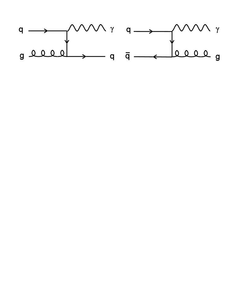
FIG. 3.: Lowest order amplitudes for photon production

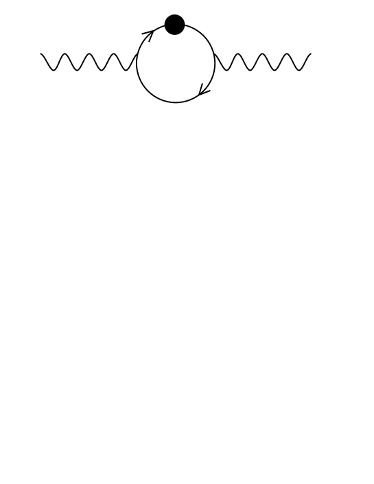
FIG. 4.: Polarization tensor containing a full quark propagator

REFERENCES

- [1] D. Nötzold and G. Raffelt, Nucl. Phys. B 307, 924 (1988)
- [2] J. Cleymans, J. Fingberg, and K. Redlich Phys. Rev. D 35, 2153 (1987)
- [3] A. Peshier and M.H. Thoma Phys. Rev. Lett. 84, 841 (2000)
- [4] E. Braaten and T.C. Yuan, Phys. Rev. Lett. 66, 2183 (1991)
- [5] R.D. Pisarski, Phys. Rev. Lett. 63, 1129 (1989); M.H. Thoma and M. Gyulassy, Nucl. Phys. B 351, 491 (1991)
- [6] P. Aurenche, F. Gelis and H. Zaraket, hep-ph/9911367
- [7] D.A. Kirzhnits, JETP Lett. 46, 308 (1987)
- [8] M.H. Thoma, hep-ph/0003016
- [9] J.D. Jackson, Classical Electrodynamics (John Wiley, New York 1975)
- [10] M. Gyulassy and M. Plümer, Phys. Lett. B 243, 432 (1990)
- [11] G.G. Raffelt, Stars as Laboratories for Fundamental Physics (University of Chicago Press, Chicago 1996)
- [12] E. Braaten and M.H. Thoma, Phys. Rev. D 44, 1298 (1991)
- [13] J.I. Kapusta, Finite Temperature Field Theory (Cambridge University Press, New York 1989)
- [14] H. Schulz, Phys. Lett. B 291, 448 (1992)
- [15] M. Leontovich, Sov. Phys. JETP 13, 634 (1961)
- [16] O.V. Dolgov, D.A. Kirzhnits, and V.V. Losyakov, Sov. Phys. JETP 56, 1095 (1982)
- [17] V.V. Klimov, Sov. Phys. JETP 55, 199 (1982); H.A. Weldon, Phys. Rev. D 26, 1394 (1982); H.A. Weldon, ibid., 2789
- [18] R. Baier, D. Schiff, and B.G. Zakharov, hep-ph/0002198
- [19] D.A. Kirzhnits, V.V. Losyakov, and V.A. Chechin, Sov. Phys. JETP 70, 609 (1990)
- [20] P.V. Ruuskanen, Nucl. Phys. A 544, 169c (1992)
- [21] J.I. Kapusta, P. Lichard, and D. Seibert, Phys. Rev. D 44, 2774 (1991)
- [22] R. Baier, H. Nakkagawa, A. Niegawa, and K. Redlich, Z. Phys. C 53, 433 (1992)
- [23] C.T. Traxler, H. Vija and M.H. Thoma, Phys. Lett. B 346, 329 (1995)
- [24] E. Braaten, R.D. Pisarski, and T.C. Yuan, Phys. Rev. Lett. 64, 2242 (1990)
- [25] H.A. Weldon, Phys. Rev. D 61, 036003 (2000)
- [26] P. Aurenche, F. Gelis, R. Kobes, and H. Zaraket Phys. Rev. D 58, 085003 (1998)