Renormalization of the Cabibbo-Kobayashi-Maskawa Matrix

Abstract

Using the on-shell scheme and the general linear $R_{\xi}$ gauge we have calculated the one-loop amplitude $W^{+}\rightarrow u_{I}\bar{d}_{j}$. In agreement with previous work we have shown that the Cabibbo-Kobayashi-Maskawa (CKM) matrix ought to be renormalized. We show how to renormalize the CKM matrix and, at the same time, obtain a gauge independent $W$ decay amplitude.

PACS number(s): 11.10.Gh, 12.15.-y, 12.15.Ff, 12.15.Lk

1 Introduction

The electroweak sector of the standard model (SM) has been the subject of extensive studies during the last twenty-five years. Since the renormalizability of the SM was proved [1] an immense effort has been made to implement this renormalization program at one-loop level (cf. ref. [2] and [3] for a review). The agreement between these calculations and the experimental results is impressive.

Despite these facts, the renormalization of the Cabibbo-Kobayashi-Maskawa (CKM) quark mixing matrix [4] was done only by one group, Denner and Sack [5] (DS) in 1990. They have shown that, as soon as one takes into account the non-degeneracy of the quark masses, the CKM ought to be renormalized. However, recently Gambino, Grassi and Madricardo [6] (GGM) have raised some doubts about the DS renormalization prescription. In particular, they have claimed that the on-shell conditions used by DS lead to a gauge dependent width for the decay $W\rightarrow q\bar{q}$. Then, they propose an alternative renormalization prescription.

In view of this situation, we decided that it is appropriate to carry out another independent calculation of the renormalization of the CKM. This is our aim. We repeat the work of DS, but with a fundamental difference. Rather than using the common ’t Hooft Feynman gauge ($\xi=1$) we do our calculation in the general linear $R_{\xi}$ gauge. Hence, we will be able to show, explicitly, the problem raised by GGM and make a proposal to solve it.

To address the question of the CKM renormalization one has to consider a process where this matrix appears at tree-level. To be precise, let us consider the decay $W^{+}\rightarrow q_{I}\bar{q}_{j}$, where $I$ and $j$ are generation indices. We use capital letters for the up-type quarks and lower case letters for the down-type quarks. Then, at tree-level the decay amplitude $T_{0}$ is

$$T_{0}=V_{Ij}A_{L}$$ (1)

with

$$A_{L}=\frac{g\,N_{c}}{\sqrt{2}}\,\bar{u}_{I}(p_{1})\mathchoice{\hbox{$\displaystyle\varepsilon\hskip-4.91493pt/\hskip 4.91493pt\hskip-5.16663pt$}}{\hbox{$\textstyle\varepsilon\hskip-4.91493pt/\hskip 4.91493pt\hskip-5.16663pt$}}{\hbox{$\scriptstyle\varepsilon\hskip-3.56958pt/\hskip 3.56958pt\hskip-3.61664pt$}}{\hbox{$\scriptscriptstyle\varepsilon\hskip-2.67274pt/\hskip 2.67274pt\hskip-2.58331pt$}}\gamma_{L}v_{j}(q-p_{1})\enskip.$$ (2)

$V_{Ij}$ are the elements of the CKM matrix, $N_{c}$ is the number of colors and $g$ is the $SU(2)$ coupling constant.

At one-loop eq. (1) is modified in several different ways. Firstly, one has to sum all one-loop irreducible vertex-diagrams. This gives a contribution proportional to $V_{Ij}$ but not entirely proportional to $A_{L}$. Secondly, we have the counter terms stemming from the usual variation of the Lagrangian parameters. The counter terms $\delta g$ and $\delta Z_{W}$ ($W$-wave function renormalization) also give rise to contributions proportional to the tree-level amplitude. However, since the quarks get mixed by the renormalization procedure, this is not true for the quark wave function renormalization constants $\delta Z_{II^{\prime}}^{L}$ and $\delta Z_{jj^{\prime}}^{L}$. Finally, an additional counter term $\delta V_{Ij}$ has to be included.

For a real $W$ that decays into on-shell quarks, it is easy to show that the vertex diagrams can be written in terms of four independent form factors. Each one is associated with a given Lorentz structure for the spinors. Denoting by $q^{\mu}$ the 4-momentum of the incoming $W^{+}$ and by $p_{1}^{\mu}$ the 4-momentum of the outgoing up-quark $I$, let us define

$$B_{L}=\frac{g\,N_{c}}{\sqrt{2}}\,\bar{u}_{I}(p_{1})\frac{\varepsilon\cdot p_{1}}{m_{W}}\gamma_{L}v_{j}(q-p_{1})\enskip,$$ (3)

where $\varepsilon^{\mu}$ is the $W$ polarization vector. Similarly, replacing in eqs. (2) and (3) $\gamma_{L}$ by $\gamma_{R}$ we define $A_{R}$ and $B_{R}$ respectively. Now, the one-loop amplitude $T_{1}$ is

$$T_{1} = A_{L}\left[\,V_{Ij}\,\left(\,F_{L}+\frac{\delta g}{g}+\mbox{$\frac{1}{2}$}\delta Z_{W}+\mbox{$\frac{1}{2}$}\delta Z_{II}^{L*}+\mbox{$\frac{1}{2}$}\delta Z_{jj}^{L}\right)\,+\,\sum_{I^{\prime}\neq I}\mbox{$\frac{1}{2}$}\delta Z_{I^{\prime}I}^{L*}V_{I^{\prime}j}\right.$$ (4)

$$\left.\phantom{A_{L}[}\,+\,\sum_{j^{\prime}\neq j}V_{Ij^{\prime}}\mbox{$\frac{1}{2}$}\delta Z_{j^{\prime}j}^{L}\,+\,\delta V_{Ij}\,\right]\,+\,V_{Ij}\,\left[\,A_{R}F_{R}+B_{L}G_{L}+B_{R}G_{R}\,\right]\enskip,$$

where $F_{L,R}$ and $G_{L,R}$ are the form-factors. We calculate the different terms in eq. (4) using the general $R_{\xi}$ gauge for the $W$-propagators. However to simplify the calculation, we use ’t Hooft-Feynman gauge for the $Z$ and photon propagators. This is not inconsistent, since the $\xi$ parameters of the gauge fixing Lagrangian,

$${\cal L}_{GF}=-\frac{1}{2\xi_{\gamma}}(\partial\!\cdot\!A)^{2}-\frac{1}{2\xi_{Z}}\left(\partial\!\cdot\!Z-\xi_{Z}m_{Z}G^{0}\right)^{2}-\frac{1}{\xi_{W}}\left|\partial\!\cdot\!W^{+}+i\xi_{W}m_{W}G^{+}\right|^{2}$$

are independent. For our purpose it is sufficient to set $\xi_{\gamma}=\xi_{Z}=1$ but to keep $\xi_{W}$ as a free parameter. From this point onwards it will be denoted simply by $\xi$. For the numerical calculations we used the values from Particle Data Group [7].

2 The irreducible vertex diagrams

Figure 1: The diagrams of the electroweak vertex corrections.

In fig. 1 we show the irreducible diagrams that give the one-loop $W^{+}\rightarrow u_{I}\bar{d}_{j}$ amplitude. The calculation of these diagrams using dimensional regularization, is standard. It was done using the xloops program [8]. To keep track of the divergences it is convenient to introduce the notation

$$\zeta=\frac{2}{D-4}-\gamma_{E}+\ln 4\pi^{2}-\ln\left(\frac{m_{W}}{\mu}\right)^{2}\enskip,$$

where $D$ is the dimension of momentum space ($D\rightarrow 4$), $\gamma_{E}$ is the Euler constant and $\mu$ is the arbitrary renormalization mass.

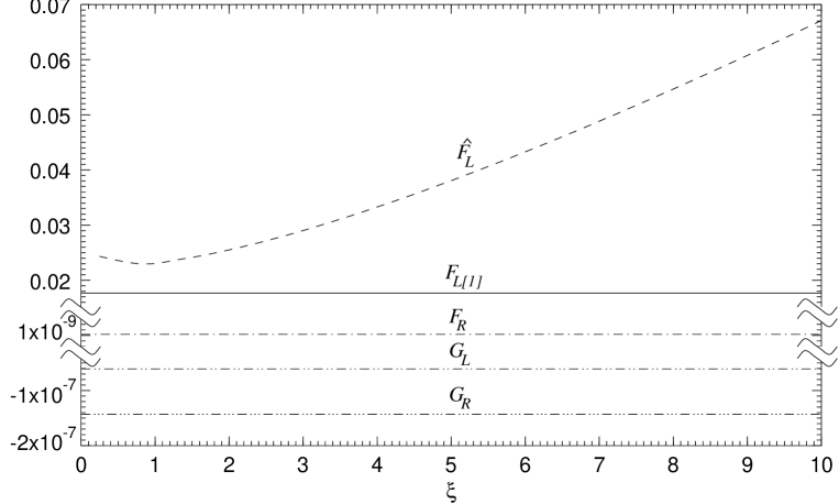
Figure 2: The real part of $F_{R}$, $G_{L}$, $G_{R}$, $\hat{F}_{L}$ and $F_{L[\mathbb{1}]}$ for the $W^{+}\!\rightarrow u\bar{d}$ decay as a function of $\xi$.

It is not particularly instructive to show in detail the form factors. So, we have decided to show explicitly the divergent contributions and plot the finite parts as a function of $\xi$. In fig. 2 we display the $\xi$ dependence of the real part of $F_{R}$, $G_{L}$ and $G_{R}$ for the decay $W^{+}\rightarrow u\bar{d}$. As one can see, these form factors are $\xi$-independent and finite as they should be. In fact, any divergence or gauge dependence here would be impossible, given the gauge structure of the theory. On the contrary, $F_{L}$ is both divergent and $\xi$ dependent, i.e.,

$$F_{L}=\frac{e^{2}}{64\pi^{2}}\,\zeta\,\left[\frac{3\xi+8}{\sin^{2}\theta_{W}}+\frac{1}{9\cos^{2}\theta_{W}}+\frac{m_{I}^{2}+m_{j}^{2}}{m_{W}^{2}}\frac{1}{\sin^{2}\theta_{W}}\right]\,+\,\hat{F}_{L}$$ (5)

where $\hat{F}_{L}$ is finite but $\xi$ dependent. This is clearly seen in fig. 2. Notice, that the form factors $F_{R}$, $G_{L}$ and $G_{R}$ are smaller than $\hat{F}_{L}$ because they are proportional to the quark masses divided by the $W$ mass.

3 The Counter terms

3.1 $W$-wave-function renormalization, $\delta Z_{W}$

Calculating the $W$-boson self-energy at one-loop and imposing the on-shell renormalization conditions one obtains [2]:

$$\delta Z_{W}=\frac{e^{2}}{96\pi^{2}\sin^{2}\theta_{W}}\,\zeta\,\left[22-3\xi-2N_{g}(1+N_{c})\right]\,+\,\delta\hat{Z}_{W}\enskip.$$ (6)

As before $\delta\hat{Z}_{W}$ denotes the finite contribution. We will follow this notation for all counter terms. $N_{g}=N_{c}=3$ are the number of generations and the number of colors, respectively. We found that it is convenient to show these parameters explicitly in order to keep track of the contributions of lepton and quark loops.

From the $W$-self-energy one also obtains the mass counter term, namely

$$\delta m_{W}^{2} = \frac{-e^{2}}{96\pi^{2}\sin^{2}\theta_{W}}\,\zeta\,\left[(34-3\xi)m_{W}^{2}-6m_{Z}^{2}-2N_{g}(1+N_{c})m_{W}^{2}\phantom{\sum_{l}}\right.$$ (7)

$$\phantom{\frac{e^{2}}{96\pi^{2}\sin^{2}\theta_{W}}\,\zeta\,[}\left.\,+\,3\sum_{l}m_{l}^{2}\,+\,3N_{c}\sum_{I^{\prime}j^{\prime}}|V_{I^{\prime}j^{\prime}}|^{2}(m_{I^{\prime}}^{2}+m_{j^{\prime}}^{2})\right]\,+\,\delta\hat{m}^{2}_{W}\enskip.$$

3.2 The coupling counter term, $\delta g$

It is discussed in great detail in ref. [2] how to obtain $\delta g$. So, again, we simply summarize our results, which agree with those in ref. [2] for $\xi=1$. It is easy to show that

$$\frac{\delta g}{g}=\frac{\delta e}{e}-\frac{\delta\sin\theta_{W}}{\sin\theta_{W}}$$ (8a)

where

$$\frac{\delta\sin\theta_{W}}{\sin\theta_{W}}=\frac{m_{W}^{2}\delta m_{Z}^{2}-m_{Z}^{2}\delta m_{W}^{2}}{2\,m_{Z}^{2}\,(m_{Z}^{2}-m_{W}^{2})}\enskip.$$ (8b)

From the $Z$-self-energy one obtains $\delta m_{Z}^{2}$. Like the analogue result shown in eq. (7), $\delta m_{Z}^{2}$ depends on $\xi$. However, the combination given by eq. (8b) is $\xi$ independent. Furthermore, $\delta e$ is also $\xi$ independent. This makes the final result

$$\frac{\delta g}{g}=\frac{e^{2}}{96\pi^{2}\sin^{2}\theta_{W}}\,\zeta\,\left[N_{g}(1+N_{c})-\frac{43}{2}\right]\,+\,\frac{\delta\hat{g}}{g}$$ (9)

fully $\xi$ independent.

3.3 The quark-fields renormalization

As it is well known, under renormalization the quark fields are mixed. Let us write the self-energy of an up-type quark in the general form:

$$\Sigma_{II^{\prime}}=\Sigma^{L}_{II^{\prime}}(p^{2})\mathchoice{\hbox{$\displaystyle p\hskip-4.6684pt/\hskip 4.6684pt\hskip-5.16663pt$}}{\hbox{$\textstyle p\hskip-4.6684pt/\hskip 4.6684pt\hskip-5.16663pt$}}{\hbox{$\scriptstyle p\hskip-3.69841pt/\hskip 3.69841pt\hskip-3.61664pt$}}{\hbox{$\scriptscriptstyle p\hskip-2.76477pt/\hskip 2.76477pt\hskip-2.58331pt$}}\gamma_{L}\,+\,\Sigma^{R}_{II^{\prime}}(p^{2})\mathchoice{\hbox{$\displaystyle p\hskip-4.6684pt/\hskip 4.6684pt\hskip-5.16663pt$}}{\hbox{$\textstyle p\hskip-4.6684pt/\hskip 4.6684pt\hskip-5.16663pt$}}{\hbox{$\scriptstyle p\hskip-3.69841pt/\hskip 3.69841pt\hskip-3.61664pt$}}{\hbox{$\scriptscriptstyle p\hskip-2.76477pt/\hskip 2.76477pt\hskip-2.58331pt$}}\gamma_{R}\,+\,\Sigma^{M}_{II^{\prime}}(p^{2})[m_{I}\gamma_{L}+m_{I^{\prime}}\gamma_{R}]\enskip.$$ (10)

Then, using the on-shell renormalization condition one obtains the matrix elements of the wave function renormalization constants $\delta Z^{L}$ [9], namely

$$\delta Z^{L}_{II}=-\Sigma^{L}(m_{I}^{2})-m_{I}^{2}\left[{\Sigma^{L}}^{\prime}(m_{I}^{2})+{\Sigma^{R}}^{\prime}(m_{I}^{2})+2{\Sigma^{M}}^{\prime}(m_{I}^{2})\right]\enskip,$$ (11a)

where ${\Sigma^{L}}^{\prime}$ denotes the derivative $\frac{\partial}{\partial q^{2}}\Sigma^{L}$, and for $I^{\prime}\neq I$

$${\delta Z^{L}_{II^{\prime}}}=2\frac{\left(m_{I}^{2}+m_{I^{\prime}}^{2}\right)\Sigma^{M}(m_{I^{\prime}}^{2})+m_{I}m_{I^{\prime}}\Sigma^{R}(m_{I^{\prime}}^{2})+m_{I^{\prime}}^{2}\Sigma^{L}(m_{I^{\prime}}^{2})}{m_{I}^{2}-m_{I^{\prime}}^{2}}\enskip.$$ (11b)

In our case we obtain:

$$\delta Z_{II}^{L}=\frac{-e^{2}}{64\pi^{2}}\zeta\,\left[\,\frac{1+2\xi}{\sin^{2}\theta_{W}}\,+\,\frac{m_{I}^{2}+\sum_{i^{\prime}}|V_{Ii^{\prime}}|^{2}m_{i^{\prime}}^{2}}{m_{W}^{2}\sin^{2}\theta_{W}}+\frac{1}{9\cos^{2}\theta_{W}}\right]\,+\,\delta\hat{Z}^{L}_{II}$$ (12a)

for the diagonal terms and

$$\delta Z_{IJ}^{L}=\frac{-e^{2}}{32\pi^{2}\sin^{2}\theta_{W}}\zeta\frac{m_{I}^{2}+2m_{J}^{2}}{m_{J}^{2}-m_{I}^{2}}\sum_{i^{\prime}}V_{Ii^{\prime}}V_{Ji^{\prime}}^{*}\frac{m_{i^{\prime}}^{2}}{m_{W}^{2}}\,+\,\delta\hat{Z}^{L}_{IJ}$$ (12b)

for the off-diagonal terms. In the latter equation a $\xi$ dependent term in the divergent part was canceled due to the unitarity of the CKM matrix. The corresponding result for the down-type quarks is:

$$\delta Z_{ij}^{L}=\frac{-e^{2}}{32\pi^{2}\sin^{2}\theta_{W}}\zeta\frac{m_{i}^{2}+2m_{j}^{2}}{m_{j}^{2}-m_{i}^{2}}\sum_{I^{\prime}}V_{I^{\prime}i}V_{I^{\prime}j}^{*}\frac{m_{I^{\prime}}^{2}}{m_{W}^{2}}\,+\,\delta\hat{Z}^{L}_{ij}$$ (13)

and the diagonal part is identical to eq. (12a) replacing $I$ by $i$ and $I^{\prime}$ by $i^{\prime}$. It is interesting to point out that the matrices $\delta Z^{L}$ are neither hermitian nor anti-hermitian. Of course, they can be decomposed in a sum of such matrices, $\delta Z^{L}=\delta Z^{LH}+\delta Z^{LA}$. However, one should realize that the divergence is present both in $\delta Z^{LH}$ and in $\delta Z^{LA}$. In fact, from eq. (12b) it is straightforward to obtain

$$\delta Z_{IJ}^{LH}=\frac{-e^{2}}{64\pi^{2}\sin^{2}\theta_{W}}\zeta\sum_{i^{\prime}}V_{Ii^{\prime}}V_{Ji^{\prime}}^{*}\frac{m_{i^{\prime}}^{2}}{m_{W}^{2}}\,+\,finite$$ (14a)

and

$$\delta Z_{IJ}^{LA}=\frac{-3e^{2}}{64\pi^{2}\sin^{2}\theta_{W}}\zeta\frac{m_{I}^{2}+m_{J}^{2}}{m_{J}^{2}-m_{I}^{2}}\sum_{i^{\prime}}V_{Ii^{\prime}}V_{Ji^{\prime}}^{*}\frac{m_{i^{\prime}}^{2}}{m_{W}^{2}}\,+\,finite\enskip.$$ (14b)

Clearly, eq. (12a) shows that the diagonal terms of $\delta Z^{L}$ are real. These remarks will be important in paragraph 5, when we consider the renormalization of the CKM matrix.

4 The $W^{+}$ decay into leptons

Using eqs. (5),(6),(9),(12a,b) and (13) it is easy to obtain:

$$F_{L}+\frac{\delta g}{g}+\mbox{$\frac{1}{2}$}\delta Z_{W}+\mbox{$\frac{1}{2}$}\delta Z_{II}^{L*}+\mbox{$\frac{1}{2}$}\delta Z_{jj}^{L}$$

$$= \frac{e^{2}}{128\pi^{2}\sin^{2}\theta_{W}}\zeta\,\frac{m_{I}^{2}-\sum_{i^{\prime}}|V_{Ii^{\prime}}|^{2}m_{i^{\prime}}^{2}+m_{j}^{2}-\sum_{I^{\prime}}|V_{I^{\prime}j}|^{2}m_{I^{\prime}}^{2}}{m_{W}^{2}}+finite\enskip.$$

Notice that there are no divergences proportional to the gauge parameter $\xi$. If $V_{Ii^{\prime}}=\delta_{Ii^{\prime}}$ and $V_{I^{\prime}j}=\delta_{I^{\prime}j}$, i.e., if the CKM matrix is the unit matrix, the divergent term is identically zero. In this case, we call the above combination of $F_{L}$ and counter terms $F_{L[\mathbb{1}]}$.

From eq. (4) it is now clear that the one-loop leptonic decay amplitude $W^{+}\rightarrow l^{+}\nu_{l}$ can be written as

$$T_{1}^{l}=A_{L}F_{L[\mathbb{1}]}+B_{R}G_{R}\enskip,$$ (16)

where in $F_{L[\mathbb{1}]}$ and $G_{R}$ the leptonic masses are used and in eq. (2) and (3) we set $N_{c}=1$. The form factors $F_{R}$ and $G_{L}$ are proportional to $m_{I}$. Hence, they vanish for massless neutrinos. As we have shown $T_{1}^{l}$ is finite, as it should be. Furthermore, fig. 2, where we show $F_{L[\mathbb{1}]}$ as a function of $\xi$, clearly proves that the one-loop leptonic amplitude $T_{1}^{l}$ is also gauge independent. Having established the finiteness and the gauge independence of $F_{L[\mathbb{1}]}$ we are now in a position to return to eq. (4) and consider the $\delta V_{Ij}$ counter term.

5 The CKM counter term

Let us consider the $W$-quark coupling in the standard model Lagrangian. Introducing an obvious matrix notation we write

$${\cal L}=-\frac{g}{\sqrt{2}}\bar{U}_{L}VD_{L}W_{\mu}+h.c.\enskip,$$ (17)

where $U_{L}$ and $D_{L}$ are the left-handed up and down quark fields respectively. Leaving aside the renormalization of $g$ and of the $W$-field, let us focus our attention in the renormalization of the quark fields and $V$. In the former work of DS the matrix $V$ is multiplicatively renormalized, i.e.

$$V\rightarrow U_{1}VU_{2}=V+\delta U_{1}V+V\delta U_{2}\enskip,$$ (18)

where $U_{1}$ and $U_{2}$ are unitary matrices. Then, introducing the usual quark wave-function renormalization,

$$\bar{U}_{L} \rightarrow \bar{U}_{L}{Z^{1/2}_{UL}}^{\dagger}$$

$$D_{L} \rightarrow Z^{1/2}_{DL}D_{L}$$

eq. (17) becomes:

$$\bar{U}_{L}VD_{L} \rightarrow \bar{U}_{L}{Z^{1/2}_{UL}}^{\dagger}U_{1}VU_{2}Z^{1/2}_{DL}D_{L}$$

$$= \bar{U}_{L}\left\{\,V\,+\,\mbox{$\frac{1}{4}$}\left[\delta Z_{UL}^{\dagger}+\delta Z_{UL}\right]V\,+\,\mbox{$\frac{1}{4}$}V\left[\delta Z_{DL}+\delta Z_{DL}^{\dagger}\right]\right.$$

$$\phantom{\left[\delta Z_{UL}^{\dagger}\right]}\,+\,\mbox{$\frac{1}{4}$}\left[\delta Z_{UL}^{\dagger}-\delta Z_{UL}\right]V\,+\,\mbox{$\frac{1}{4}$}V\left[\delta Z_{DL}-\delta Z_{DL}^{\dagger}\right]$$

$$\left.\phantom{\left[\delta Z_{UL}^{\dagger}\right]}\,+\,\delta U_{1}V\,+\,V\delta U_{2}\,\right\}\,D_{L}\enskip,$$

where, for convenience, we have split the $\delta Z$ matrices into its hermitian and anti-hermitian parts. Because the unitarity of the matrices $U_{i}$ implies that the $\delta U_{i}$ are anti-hermitian, DS concluded that $\delta V=\delta U_{1}V+V\delta U_{2}$ is required to absorb the divergence in the anti-hermitian parts of $\delta Z_{L}$. Hence, they have introduced the following renormalization condition:

$$\delta V=-\mbox{$\frac{1}{4}$}\left[\delta Z_{UL}^{\dagger}-\delta Z_{UL}\right]V\,-\,\mbox{$\frac{1}{4}$}V\left[\delta Z_{DL}-\delta Z_{DL}^{\dagger}\right]\enskip.$$ (20)

Of course, there are still divergences in the hermitian part of $\delta Z$, but, as we will see, they are the ones needed to cancel the divergences in the vertex contribution to $F_{L}$. In fact, using eqs. (14a,b) and (12a,b) it is straightforward to obtain:

$$\mbox{$\frac{1}{2}$}\left[\delta Z_{UL}^{H}V+V\delta Z_{DL}^{H}\,\right]_{Ij} = \frac{-e^{2}}{128\pi^{2}\sin^{2}\theta_{W}}\zeta\,\left[\sum_{i^{\prime}J}V_{Ii^{\prime}}V_{Ji^{\prime}}V_{Jj}\frac{m_{i^{\prime}}^{2}}{m_{W}^{2}}\,+\,\frac{m_{I}^{2}}{m_{W}^{2}}V_{Ij}\right.$$ (21)

$$\left.\qquad\,+\,\sum_{I^{\prime}i^{\prime}}V_{Ii^{\prime}}V_{I^{\prime}i^{\prime}}V_{I^{\prime}j}\frac{m_{I^{\prime}}^{2}}{m_{W}^{2}}\,+\,\frac{m_{j}^{2}}{m_{W}^{2}}V_{Ij}\,\right]\;+\;finite\enskip.$$

In the equation above, when using the diagonal elements of the matrix $\delta Z^{H}$, only the contribution of the second term of eq. (12a) is explicitly shown. The other two terms are irrelevant for the discussion since they cancel with similar divergences coming from $F_{L}$, $\delta Z_{W}$ and $\delta g$.

Now, the unitarity of $V$ reduces eq. (21) to the form:

$$\mbox{$\frac{1}{2}$}\left[\delta Z_{UL}^{H}V+V\delta Z_{DL}^{H}\,\right]_{Ij}=\frac{-e^{2}}{64\pi^{2}\sin^{2}\theta_{W}}\zeta\,\frac{m_{I}^{2}+m_{j}^{2}}{m_{W}^{2}}\,V_{Ij}\enskip,$$ (22)

which is exactly what we need to cancel a similar divergence in $V_{Ij}F_{L}$, namely the third term in eq. (5).

Hence, from the point of view of canceling the divergences in $T_{1}$, the renormalization proposal by DS works. In other words, it is sufficient to choose $\delta V$ as the divergent part of the right hand side of eq. (20) to obtain a finite one-loop amplitude. DS have also included in $\delta V$ the finite contributions stemming from $\delta Z^{A}$. We have checked that this gives rise to a gauge dependent result.

To solve this problem let us define the quantity

$$\delta X_{ud} = \mbox{$\frac{1}{2}$}V_{ud}\left[\delta Z_{uu}^{L*}-\delta Z_{uu[\mathbb{1}]}^{L*}+\delta Z_{dd}^{L}-\delta Z_{dd[\mathbb{1}]}^{L}\right]$$ (23)

$$+\mbox{$\frac{1}{2}$}\sum_{I^{\prime}\neq u}\delta Z^{L*}_{I^{\prime}u}V_{I^{\prime}d}+\mbox{$\frac{1}{2}$}\sum_{j^{\prime}\neq d}V_{uj^{\prime}}\delta Z^{L}_{j^{\prime}d}\enskip,$$

which obviously represents the difference between the “leptonic” and the quark transition amplitude. Notice that $\delta Z_{uu[\mathbb{1}]}^{L*}$ is given by eq. (12a) but replacing the CKM by the unit matrix. After introducing the quantity $\delta X_{Ij}$ it is clear that eq. (4) can be rewritten as

$$T_{1}=V_{Ij}\left[A_{L}F_{L[\mathbb{1}]}+A_{R}F_{R}+B_{L}G_{L}+B_{R}G_{R}\right]+A_{L}\left[\delta X_{Ij}+\delta V_{Ij}\right]\enskip.$$ (24)

Having proved that the first term of eq. (24), proportional to $V_{Ij}$, is both finite and gauge independent, it is obvious that the CKM counter term should be

$$\delta V_{Ij}=-\delta X_{Ij}\enskip.$$ (25)

This is our main result. On physical terms what we are saying is that all contributions to the $T_{1}$ amplitude arising from the renormalization of the quark mixing are canceled by the CKM counter term. This $\delta V$ is an alternative to the one proposed by GGM which requires the use of quark wave function renormalization constants at zero momentum. Both schemes lead to gauge invariant results. In fact, the unitarity of the CKM matrix implies that $\delta X$ is gauge independent.

6 Conclusions

Beyond tree-level, quarks with the same electric charge get mixed under renormalization. Then, the amplitude for the $W^{+}\rightarrow u\bar{d}$ explicitly depends on these flavor-changing renormalization constants. Therefore, to obtain a finite amplitude it is essential to renormalize the corresponding element of the CKM matrix, $V$. Using the on-shell renormalization scheme and the $R_{\xi}$ gauge we have shown how to construct the CKM counter term matrix $\delta V$. Our final result is given in eq. (25). With this prescription the tree-level relation

$$T(W^{+}\rightarrow u\bar{d})=V_{ud}N_{c}T(W^{+}\rightarrow e^{+}\nu_{e})\enskip,$$

living aside $\alpha_{s}$ corrections and obvious kinematic differences, is maintained at the next order. We have proved that at one-loop one obtains a finite and gauge independent amplitude. It is interesting to point out that a finite amplitude $T_{1}$ can only be obtained, if the CKM matrix is unitary. This is particular important in view of some recent discussions about a possible non-unitarity of this matrix [10].

7 Acknowledgement

We thank Paolo Gambino for pointing out an error in a previous version of this work. This work is supported by Fundação para a Ciência e Tecnologia under contract No. CERN/P/FIS/15183/99. L.B. is supported by JNICT under contract No. BPD.16372.

References

- [1] G. ’t Hooft and M. Veltman, Nucl. Phys. B44 (1972) 189 ; G. ’t Hooft and M. Veltman, Nucl. Phys. B50 (1972) 318.
- [2] K. I. Aoki, Z. Hioki, M. Konuma, R. Kawabe, and T. Muta, Prog. Theor. Phys. Suppl. 73 (1982) 1.
- [3] M. Böhm, H. Spiesberger, and W. Hollik, Fortsch. Phys. 34 (1986) 687.
- [4] N. Cabibbo, Phys. Rev. Lett. 10 (1963) 531 ; M. Kobayashi and T. Maskawa, Prog. Theor. Phys. 49 (1973) 652.
- [5] A. Denner and T. Sack, Nucl. Phys. B347 (1990) 203.
- [6] P. Gambino, P. A. Grassi, and F. Madricardo, Phys. Lett. B454 (1999) 98.
- [7] C. Caso et al., Eur. Phys. J. C3 (1998) 1.
- [8] L. Brücher, J. Franzkowski, and D. Kreimer, Comput. Phys. Commun. 115 (1998) 140 ; L. Brücher, Nucl. Instrum. Meth. A389 (1997) 327 ; L. Brücher, J. Franzkowski, and D. Kreimer, hep-ph/9710484.
- [9] J. M. Soares and A. Barroso, Phys. Rev. D39 (1989) 1973.
- [10] C. Kim and H. Yamamoto, hep-ph/0004055.