hep-ph/0004130 April 2000 OUTP–00–15P
A Brane–World Explanation of the KARMEN Anomaly

Abstract

Motivated by the anomaly in the KARMEN experiment, we study new possibilities for brane–world models of neutrino masses. We show that the KARMEN anomaly can be understood in the context of a six–dimensional brane–world model. The fine–tuning problem associated with the single–particle interpretation of the anomaly is thereby alleviated. Our model shows some interesting properties of general interest for brane–world neutrino physics. In particular, the size of the brane–bulk mixing decouples from the scales relevant for atmospheric and solar neutrino oscillations.

1 Introduction

Two recent developments, namely the discovery of brane–world models [1, 2, 3, 4, 5, 6, 7] and the flexibility in choosing fundamental scales and sizes of additional dimensions [2, 8, 5, 6], have led to considerable activity exploring new options for particle phenomenology. Both developments have a natural place in string– or M–theory which leads to interesting connections between the leading candidate for a fundamental theory and particle physics.

Much of the interesting phenomenology of brane–world models is associated with the Kaluza–Klein modes that originate from large, gravity–only additional dimensions. Particularly the graviton and its Kaluza–Klein excitations are of interest in this context [5]. Neutrino physics is another branch that is likely to be effected in brane–world models. This is because higher–dimensional bulk fermions lead to Kaluza–Klein towers of standard model singlets that may be interpreted as sterile neutrinos [9, 10, 11, 12]. Most of the work in brane–world neutrino physics to date has been focusing on rather specific models. Concretely, most of the explicit studies have been carried out for simple five–dimensional models with a special form of the action that, for example, does not include bulk mass terms (see, however, ref. [9], where Majorana mass terms have been considered in the context of orbifold models).

Brane–world models with large additional dimensions have led to a number of exciting predictions, such as the modification of gravity at small distances [5], that may be testable in the future. In this paper, we would like to pursue the idea that a signal originating from brane–world physics may have already been observed. Specifically, we will show that the anomaly in the KARMEN neutrino experiment [13, 14] can be explained in the context of brane–world models. This will also lead us to explore new possibilities for brane–world models of neutrino masses. That is, we will examine a number of new model building aspects in brane–world theories of neutrino masses.

The KARMEN neutrino experiment studies neutral current interactions of neutrinos that originate from the decay chain $\pi^{+}\rightarrow\mu^{+}$ at rest. The KARMEN experiment has a unique time structure that allows one to study the number of neutrino events in the detector as a function of time after the production of the initial $\pi^{+}$. It is this distribution that shows an anomalous peak at a specific time after $\pi^{+}$ production. The KARMEN anomaly can be explained in terms of a hypothetical $X$ particle [13] produced in a rare decay $\pi^{+}\rightarrow\mu^{+}X$. It has also been shown [15] that the $X$ particle can be interpreted as a sterile neutrino. While postulating such a particle leads to a satisfactory fit of the experimental data it has a theoretically unappealing feature. To match the observed peak, the $X$ particle has to have a very specific mass $m_{X}$ that is fine–tuned to the mass difference $m_{\pi}-m_{\mu}$ with an accuracy of approximately $10^{-4}$. That is, $m_{X}/(m_{\pi}-m_{\mu})\simeq 1-1.8\,10^{-4}$. There is no apparent theoretical explanation for such a coincidence of masses.

Here is where brane–world physics might come into play. Suppose, that a brane–world model leads to a Kaluza–Klein tower of sterile neutrinos. Clearly, if the spacing is sufficiently small, it is relatively more probable for one of the particles in this tower to fall into the narrow mass range relevant for the KARMEN experiment than it is for a single particle. In the extreme case, where the spacing of the tower is of the order of the mass gap available for the $X$ particle, the fine–tuning problem is solved completely.

In this paper, we will show that a brane–world model explaining the KARMEN anomaly does indeed exist. An analysis of the basic requirements singles out two specific choices of dimensions and scales. The first one corresponds to a five–dimensional model with intermediate string scale and the scale of the fifth dimension in the $\,\mathrm{keV}$ range. The second one corresponds to a six–dimensional model with a $\,\mathrm{TeV}$ string scale and the scale of the two additional dimensions in the $\,\mathrm{MeV}$ range. We will focus on the second case and construct an explicit six–dimensional model that meets all the requirements. A major phenomenological constraint on this model is that the other Kaluza–Klein sterile neutrinos do not distort the KARMEN spectrum in a way inconsistent with the experiment. We will show that this can be avoided by making the spacing of the Kaluza–Klein tower sufficiently large. Unfortunately then, the fine–tuning problem cannot be solved completely in the way indicated above but is still improved by two orders of magnitude with respect to the single particle interpretation. At the same time, the effect of the Kaluza–Klein modes lighter than the $X$ particle, provide a way of how our proposal could be experimentally distinguished from the single particle proposal. These particles contribute to the KARMEN spectrum at short times and, depending on the parameters of the model, the corresponding signal may be detectable in future experiments.

Our six–dimensional model also shows a number of interesting properties that are of general importance for brane–world models of neutrino masses. In the simplest version of the model with conserved lepton number, for example, we find three massless eigenstates that are generally nontrivial linear combinations of the electroweak eigenstates and the bulk neutrinos. The admixture of bulk neutrinos is controlled by a six–dimensional Dirac mass and can be made small or large while keeping the states massless. In contrast, in the models considered so far, massless modes were either not present or decoupled from the ordinary neutrinos. Furthermore, in those models, light neutrino masses and their mixing with bulk neutrinos are usually controlled by the same parameters. Our model shows that it is actually possible to decouple these two quantities. More generally, it is illustrated that the inclusion of all Lorenz–invariant (or even Lorenz non–invariant) mass terms in the higher–dimensional theory opens up new possibilities for brane–world neutrino phenomenology.

2 The KARMEN anomaly and its brane–world interpretation

The KARMEN experiment at the Rutherford Appleton Laboratory studies charged and neutral current interactions of neutrinos from the $\pi^{+}\rightarrow\mu^{+}$ decay chain at rest. The unique feature of the neutrino flux is its time structure. The primary pions are produced in $0.5\,\mathrm{\mu s}$ long pulses with a frequency of $50\,\text{Hz}$ by the ISIS synchrotron proton beam. Due to the short pion lifetime, $\tau_{\pi}\simeq 26\,\mathrm{ns}$, the muon neutrinos from the $\pi^{+}\rightarrow\mu^{+}\nu_{\mu}$ decay represent the prompt component of the neutrino beam, which exhausts itself within a few $\tau_{\pi}$ after the pion pulse. Hence, in the time window $(0.6$–$10.6)\,\mathrm{\mu s}$ after proton beam on target the neutrino beam is exclusively composed out of $\nu_{e}$ and $\bar{\nu}_{\mu}$ that originate from the slow decay ($\tau_{\mu}\simeq 2.2\,\mathrm{\mu s}$) of the muons produced in the first $0.5\,\mathrm{\mu s}$. Consequently, the time spectrum of the number $n$ of detector events in this time window is expected to be described by

$$\frac{dn}{dt}=Ae^{-t/\tau_{\mu}}+B\;.$$ (1)

Here $A$ is a time–independent rate constant depending, among other things, on the muon production rate, on the target cross section and on the detector efficiency. The constant $B$ represents the event rate associated with a time–independent background.

The KARMEN time–anomaly [13, 14] manifests itself in a discrepancy between the expected time spectrum (1) and the measured one. This discrepancy is mainly due to a peak at approximately $3.6\,\mathrm{\mu s}$ after beam on target. Such a peak is clearly visible in Fig. 1a. In this plot the time window $(0.6\,\text{--}\,10.6)\,\mathrm{\mu s}$ has been divided into 20 bins and the number of events for each bin (falling into the energy range from $10$ to $36\,\mathrm{MeV}$) has been indicated by a dot. In order to estimate the significance of the discrepancy and for later comparison with results based on our model we have performed a simple analysis of the data shown in Fig. 1a. Specifically, we have carried out a $\chi^{2}$ fit of the data set in Fig. 1 assuming an event rate as in eq. (1). Background measurements on a wider time interval fix the parameter $B$ as indicated by the dashed line in Fig. 1. The best fit results in $\chi^{2}_{\text{min}}=29$ for 19 degrees of freedom, corresponding approximately to a $2\sigma$ discrepancy. However, the significance of the discrepancy is higher if one considers only the two bins around $t=3.6\,\mathrm{\mu s}$. This is appropriate because an explanation of the anomaly around $t=3.6\,\mathrm{\mu s}$ by statistical fluctuation is strongly disfavored. The peak around $t=3.6\,\mathrm{\mu s}$, already clearly present in the 1995 data [13], has, in fact, been confirmed by the subsequent KARMEN2 data [14]. Once the two bins around $t=3.6\,\mathrm{\mu s}$ have been excluded, the remaining data is very well described by the distribution in eq. (1). The best fit leads to $\chi^{2}_{\text{min}}=14$ with 17 degrees of freedom, corresponding to the solid line in Fig. 1a. According to such a fit, a total of 557 events are expected in the two unfitted bins. As shown in [14], the measured 659 events represent a deviation at the level of approximately $4\sigma$. Since the time–anomaly appears to be statistically significant and any attempt to explain its peak structure by systematic effects failed so far, it is worth to speculate about its physical origin.

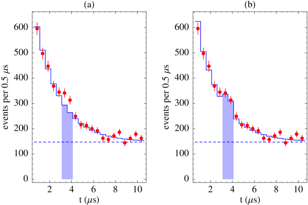
Figure 1: Time distribution of events in the time window $(0.6\,\text{--}\,10.6)\,\mathrm{\mu s}$ after beam on target and in the energy interval $(10\,\text{--}\,36)\,\mathrm{MeV}$. The time interval is divided in 20 bins. The dots represent the measured events. The dashed line indicates the measured background. In Figure (a) the solid histogram shows the best fit of all bins except the 6th and the 7th (shadowed bins) using the event rate in eq. (1). In Figure (b) the signal associated with a Kaluza–Klein tower of states corresponding to $1/R\sim 15\,\mathrm{MeV}$ is added (see text).

A simple description of the time spectrum can be achieved by assuming that the peak around $t=3.6\,\mathrm{\mu s}$ is associated with the decay of a slowly moving massive neutral particle “$X$” in the detector. Such a particle could, for example, be produced in the rare decay $\pi^{+}\rightarrow\mu^{+}X$ [13]. The position of the peak then measures the time of flight of the particle and hence its velocity. According to the recent KARMEN fits [14] the velocity is given by $\beta_{X}\simeq 0.0162$. This velocity, in turn, determines the time the particle spends in the detector and, together with the time structure of the proton beam, the width of the signal. This width is found to be in nice agreement with the observed width of the peak. More generally, the slow particle interpretation is supported by a detailed analysis of the whole data set. Due to the very good time and spatial resolution of the detector, $\Delta t<2\,\mathrm{ns}$, $\Delta x$, $\Delta y$, $\Delta z<15\,\text{cm}$, an analysis of the correlation between time and position of the events is possible. Such an analysis is in agreement with the slow particle hypothesis and provides the most precise measurement of the $X$ particle velocity leading to the value given above [14].

Once the signal is attributed to the decay of a slow particle, a rare $\pi^{+}\rightarrow\mu^{+}X$ decay represents the simplest possibility for the production of the particle. Since the time width of the anomaly is smaller than the muon lifetime, it is natural to assume that its production is not associated to muon decay (see however [16]). Moreover, the production in the $\pi^{+}$ decay allows to account for the slow, fixed velocity in terms of a small available phase space (unlike, for example, the production by the proton interactions with the target). Finally, the energy deposited by the particle in the detector is found to be less than about $35\,\mathrm{MeV}$ [14]. This is what is expected from the decay of a particle produced in the decay $\pi^{+}\rightarrow\mu^{+}X$, whose mass $m_{X}$ has to be less than $m_{\pi}-m_{\mu}\simeq 33.9\,\mathrm{MeV}$. On the other hand, if the production process were $\pi^{+}\rightarrow e^{+}X$, the slow $X$ particle would have to have a mass $m_{X}\simeq 137\,\mathrm{MeV}$ and would release more energy than measured (unless having a muon or another massive particle in the final state is for some reason favored). As for the decay, the simplest possibilities for the visible decay of a particle produced in the $\pi^{+}\rightarrow\mu^{+}X$ channel are $X\rightarrow e^{+}e^{-}\nu$ and $X\rightarrow\gamma\nu$, where $\nu$ generically represents a neutral light particle. A visible decay mainly through $X\rightarrow\gamma\nu$ thereby producing mono–energetic photons is highly disfavored [14]. Consequently, in this paper we will consider the possibility that the $X$ particle is produced in the decay $\pi^{+}\rightarrow\mu^{+}X$ decay and the anomaly is mainly due to its visible decay $X\rightarrow e^{+}e^{-}\nu$. If the $X$ particle lifetime is larger than $3.6\,\mathrm{\mu s}$, as it will be in our case, the KARMEN data requires that

$$\text{BR}(\pi^{+}\rightarrow\mu^{+}X)\cdot\Gamma_{\text{vis}}=(1\,\text{--}\,2)\,10^{-11}\,\text{s}^{-1},$$ (2)

where $\text{BR}(\pi^{+}\rightarrow\mu^{+}X)$ is the branching ratio of the decay $\pi^{+}\rightarrow\mu^{+}X$ and $\Gamma_{\text{vis}}$ is the partial width of the visible $X$ decays.

The first proposal for the nature of the hypothetical $X$ particle was made in [15]. There, it was identified with a sterile neutrino that mixes with the Standard Model (SM) neutrinos. The same possibility was considered in [17, 18]. Supersymmetric scenarios were studied in [19, 20]. From a theoretical point of view, light sterile neutrinos are welcome if their lightness can be accounted for. Whereas the mass of the SM neutrinos is protected by the electroweak symmetry (and the absence of fundamental isovector Higgses), the SM symmetries alone cannot explain why sterile neutrinos should be lighter than, say, the Planck mass. It is therefore useful to consider sterile neutrinos in the context of a specific framework. In this paper, we will be dealing with sterile neutrinos that arise in brane–world models with large additional dimensions. Concretely, we consider the possibility that the KARMEN anomaly is due to a sterile neutrino that is part of a tower of Kaluza–Klein excitations associated with a SM–singlet fermion propagating in $4+d$ dimensions. A possible explanation for small sterile neutrino masses is available if these models are viewed in the context of string theory. Then, bulk fermions arise naturally as superpartners of moduli fields. Perturbatively, moduli are flat directions of the theory, and, hence, their fermionic partners are massless before supersymmetry breaking. After including supersymmetry breaking effects those fermions will receive a mass related to the supersymmetry breaking scale. Depending on the details, this might well provide a reason for small bulk fermion masses. The next sections will be devoted to a detailed study of such models, particularly in six dimensions. In the remainder of this section, we will describe some general features of our six–dimensional model from a phenomenological viewpoint and summarize its implications for the KARMEN experiment.

Let us consider six–dimensional Dirac fermions as the origin of the sterile neutrinos. For simplicity we will consider only one such Dirac fermion here, although our later treatment will be more general. From a four–dimensional perspective, this field can be described by a Kaluza–Klein tower of sterile Dirac neutrinos $\nu_{n}$ labeled by two integer numbers $n=(n_{1},n_{2})$. Assuming, for simplicity, that the two extra dimensions have equal size $2\pi R$, the mass spectrum of the Kaluza–Klein tower is given by by

$$m_{n}=\sqrt{\mu^{2}+\frac{n^{2}}{R^{2}}},$$ (3)

where $n^{2}=n_{1}^{2}+n_{2}^{2}$ and the mass parameter $\mu$ originates from a six–dimensional Dirac mass term. Of course, to have a candidate for the $X$ particle among these Kaluza–Klein fermions we have to require that the mass parameter $\mu$ is smaller than mass $m_{X}$ of the $X$ particle. This requirement precisely corresponds to the problem of keeping sterile neutrinos light. With the above string theory explanation for this in mind, we assume that $\mu<m_{X}$. Then, we may have a specific sterile neutrino $X=\nu_{n_{X}}$ in the Kaluza–Klein tower that we would like to associate with the KARMEN anomaly. From eq. (3) we can compute the density of states $\rho(m_{X})$ at the scale $m_{X}$, defined as the average number of states $dn$ per mass interval $dm$. Neglecting the mass $\mu$ for an order of magnitude estimate, this density can be computed from eq. (3) to be 

$$\rho(m_{\rm X})\simeq 2\pi R^{2}m_{\rm X}\;.$$ (4)

In other words, the average separation between two subsequent states at $m_{\rm X}$ in a mass–ordered list is given by

$$\Delta m_{\text{KK}}=\frac{1}{\rho(m_{\rm X})}\simeq\frac{1}{2\pi R^{2}m_{\rm X}}.$$ (5)

The last equation highlights an interesting feature of our framework. Besides being able to account for the existence of light sterile neutrinos, it allows us to alleviate the fine–tuning problem associated with the slow particle interpretation of the KARMEN anomaly. The fine–tuning problem arises because the slowness of the $X$ particle requires its mass to be only slightly lower than the difference $m_{\pi}-m_{\mu}\simeq 33.9\,\mathrm{MeV}$. More precisely, in order to be produced with a velocity $\beta_{X}\simeq 0.0162$, the $X$ particle mass $m_{X}$ must be

$$m_{X}=m_{\pi}-m_{\mu}-\delta m_{X},$$ (7)

where

$$\delta m_{X}\simeq\beta^{2}_{X}\,(m_{\pi}-m_{\mu})\frac{m_{\pi}}{2m_{\mu}}\simeq 6\,\mathrm{keV}.$$ (8)

This means that $m_{X}$ is fine tuned to the $m_{\pi}-m_{\mu}$ mass difference with a precision of $1.8\times 10^{-4}$! On the other hand the fine tuning problem is significantly alleviated in the approach we propose, since the $X$ particle is just one of the many excitation of the six–dimensional fermion. It is therefore relatively more probable that one out of the many states has a mass that falls into the critical range.

In principle, this framework allows us to completely eliminate the fine tuning problem. In fact, the problem disappears if the average separation between subsequent states is about twice the mass range available for the $X$ particle, that is, $\delta m_{X}=m_{\pi}-m_{\mu}-m_{X}\sim\Delta m_{\text{KK}}/2$. From eq. (5) this happens if

$$\frac{1}{R}=(2\pi m_{X}\Delta m_{\text{KK}})^{1/2}\sim(4\pi m_{X}\delta m_{X})^{1/2}\simeq 1.6\,\mathrm{MeV}.$$ (9)

In this case, the production of the particles heavier than $X$ in the $\pi^{+}\rightarrow\mu^{+}\nu_{n}$ decay would be kinematically forbidden. However, the states lighter than $m_{\rm X}$, being faster than the $X$ particle, modify the time spectrum in the window $(0.6\,\text{--}\,3.6)\,\mathrm{\mu s}$. In order compute the effect of those lighter states on the time spectrum, one has to take into account that they are produced more copiously due to the larger phase space available. However, their signal is shorter because they spend less time inside the detector. A simulation taking into account the detailed time–shape of the signal associated with the lighter particles shows that the KARMEN data is in very good agreement with the mass spectrum associated with an inverse radius of about $15\,\mathrm{MeV}$, namely about 10 time larger than the natural value in (9). Fig. 1b shows the corresponding best fit (solid line). Once the mass spectrum has been fixed by the choice of $1/R$, the overall normalization of the sterile neutrinos signal and the constant $A$ in eq. (1) are fitted to the data. The best fit shown in Figure has a $\chi^{2}_{\text{min}}=15.8$ for 18 degrees of freedom. The fine tuning problem is alleviated. The maximum density of states at the $m_{X}$ scale is about 40 times larger than $(m_{\pi}-m_{\mu})^{-1}$, making this framework about 40 times more natural than the standard framework with a single particle. However, a significant fine tuning is still needed.

The discussion above points out a peculiar feature of our proposal. The $X$ particle comes with a number of particles lighter than $m_{X}$ whose number depends on the radius of the additional dimensions. For large values of the inverse radius, the lighter states are separated by a large mass gap. In this case our model is indistinguishable from models with a single sterile neutrino as far as the KARMEN experiment is concerned. However, from the theoretical point of view, it still provides a well motivated scenario for the existence of a sterile neutrino with a mass of $33.9\,\mathrm{MeV}$ which, at the same time, can account for the standard oscillation phenomenology (see Section 4). On the other hand, if the average mass gap $\Delta m_{\text{KK}}$ between the states is smaller than about $5\,\mathrm{MeV}$, the particles lighter than $X$ could give a small contribution to the early KARMEN time spectrum. For example, with the parameters used for the fit shown in Fig. 1b, corresponding to an average separation of about $1\,\mathrm{MeV}$ between states, one gets a small contribution to the number of events in the first time bin. Therefore, a detailed study of the time distribution at early times after the end of the proton pulse could test the model if the mass separation $\Delta m_{\text{KK}}$ happens not to be too large. An upgraded detector with tracking capability devoted to the study of the anomaly could certainly explore this possibility. Needless to say, the detection of a signal at early times would represent a strong hint for the existence of a brane–world.

3 Scales and couplings

In this section, we would like to analyze the scales and couplings of the brane–world theory that are required for a solution of the KARMEN anomaly along the lines explained above. This analysis will provide us with an overview over the various models that may be suitable for our purpose. In the following section, we will pick one of the models found in this way and develop it in detail.

We start with a ten–dimensional string theory with string scale $M_{\rm s}$. The six internal dimensions are schematically divided into two groups. The first group of $d$ dimensions are the ones that give rise to Kaluza–Klein neutrinos potentially relevant for the KARMEN experiment. The other $6-d$ dimensions are those without any direct relevance for the experiment. For example, a particular dimension is not relevant in this sense if its inverse size is much larger than the mass of the $X$ particle. For simplicity we assume that the first $d$ dimensions have the same size characterized by the radius $R$. This is likewise assumed for the remaining $6-d$ dimensions where the corresponding radius is called $\rho$. Given this setup, there are three basic requirements to be satisfied. First, the four–dimensional Planck constant $M_{\text{Pl}}$ specified by

$$\left(\frac{M_{\text{Pl}}}{M_{\rm s}}\right)^{2}=16\pi(2\pi RM_{\rm s})^{d}(2\pi\rho M_{\rm s})^{6-d}$$ (10)

should have the correct value. Except for this general condition we have two more constraints that are specific to our problem. The first one is related to the probability of having a Kaluza–Klein particle with mass in the relevant range for the slow–particle interpretation of the KARMEN experiment. We would like to significantly reduce the amount of fine tuning required. This means that the parameter $\Delta$ defined as

$$\frac{1}{\Delta}=\rho(m_{\rm X})\Delta m_{\text{KK}}\;$$ (11)

should be significantly smaller than $\mathcal{O}\left(10^{4}\right)$, corresponding to the fine–tuning of the single–particle solution. We remind the reader that $\rho(m_{\rm X})$ is the density of Kaluza–Klein states at $m_{X}=33.9\,\mathrm{MeV}$ and $\Delta m_{\text{KK}}\simeq 6\,\mathrm{keV}$ is the mass gap between the $X$ particle mass and the $\pi$-$\mu$ mass difference. Note that, from the distinction of dimensions made above, only the Kaluza–Klein modes associated to $d$ dimensions are relevant for this density. For $N$ Dirac spinors in $4+d$ dimensions with a Dirac mass $\mu$ it is given by

$$\rho(m_{\rm X})=\frac{d\,2^{[d/2]}\pi^{d/2}}{\Gamma(d/2+1)}NR^{d}m_{\rm X}(m_{\rm X}^{2}-\mu^{2})^{d/2-1}\;.$$ (12)

The final requirement originates from the constraint (2) on the branching ratio and the visible decay width of the $X$ particle. This constraint implies that there should be a non–negligible mixing between the $X$ particle and the left–handed neutrinos. In the models under consideration such a mixing is generated by a mass term between brane and bulk fields that resides on the brane. On dimensional grounds the associated mass parameter ${\hat{m}}$ can be written as

$${\hat{m}}=\frac{hv}{(2\pi RM_{\rm s})^{d/2}}=\frac{hm_{t}}{h_{t}(2\pi RM_{\rm s})^{d/2}}\;,$$ (13)

where $h$ is a brane–bulk Yukawa coupling, $v$ is the the standard model Higgs VEV and $h_{t}$ and $m_{t}$ are the top Yukawa–coupling and mass. Then, the mixing matrix element $U_{\nu X}$ between the left–handed neutrinos and the $X$ particle specified by

$$U_{\nu X}=\frac{{\hat{m}}}{m_{X}}$$ (14)

should not be too small. Typically, from eq. (2) one has $|U_{\nu X}|\simeq 10^{-3}$.

Altogether, we now have three constraints for our three fundamental parameters $M_{\rm s}$, $R$ and $\rho$. All other quantities appearing in those constraint are either fixed or in a well–defined range. We can therefore simply solve for $M_{\rm s}$, $R$ and $\rho$ as a function of the number of dimensions $d$. The fact that we can basically determine all fundamental scales is quite remarkable and shows how constrained the problem is. A priori, it is not clear at all that a solution with sensible values of the scales exists. However, as Table 1 shows, this is indeed the case. The quantity $y$ appearing in the table is defined as

$$y=\frac{h}{10^{3}|U_{\nu X}|h_{t}}\;.$$ (15)

	$(N\Delta y^{2})^{-1/d}\times$	$(N\Delta)^{-1/d}\times$	$(N\Delta)^{\frac{d-8}{d(6-d)}}y^{\frac{-16}{d(6-d)}}\times$
	$M_{\rm s}$	$R^{-1}$	$\rho^{-1}$
$d=1$	$4.5\times 10^{7}\,\mathrm{GeV}$	$12\,\mathrm{keV}$	$7.9\times 10^{6}\,\mathrm{GeV}$
$d=2$	$1.2\,\mathrm{TeV}$	$1.6\,\mathrm{MeV}$	$461\,\mathrm{MeV}$
$d=3$	$23\,\mathrm{GeV}$	$5.6\,\mathrm{MeV}$	$28\,\mathrm{keV}$

Table 1: Shown are scales and dimensions relevant for an explanation of the KARMEN experiment. We present typical values of the string scale $M_{\rm s}$, the inverse radius $R^{-1}$ of the $d$ additional dimensions associated with relevant Kaluza–Klein neutrinos and the inverse radius $\rho^{-1}$ of the remaining $6-d$ dimensional internal space.

Let us discuss the various cases shown in table 1. For one additional dimensions $d=1$, we have a model with intermediate string scale, one large additional dimension in the $\,\mathrm{keV}$ range and the size of the other five dimensions close to the string scale. For two additional dimensions, $d=2$, the situation is quite different. We have a model with the string scale in the $\,\mathrm{TeV}$ range, two large additional dimensions in the $\,\mathrm{MeV}$ range and the scale of the other four internal dimensions being about two to three orders of magnitude larger. In the case of three additional dimensions, $d=3$, the typical string scale is already quite low and one needs a large factor $N\Delta y^{2}$ to elevate it above the required $\,\mathrm{TeV}$ limit. Therefore, this case only represents a marginal possibility. Finally, one can show that models with more than three additional dimensions, $d>3$, lead to a string scale below $\,\mathrm{TeV}$ and are, therefore, not viable in our context.

In summary, we have isolated two cases which may lead to an explanation of the KARMEN anomaly in the context of a brane–world model. The first case represents an effective five–dimensional model with intermediate string scale and the remaining five dimensions being close to the string scale. The second one is a model with a $\,\mathrm{TeV}$ string scale, two large dimensions in the $\,\mathrm{MeV}^{-1}$ range and the scale of the remaining four dimensions being two to three orders of magnitude larger. Therefore, this model is effectively six–dimensional in an intermediate energy range. We stress that the existence of these two possibilities, particularly the one with a $\,\mathrm{TeV}$ string scale, was by no means guaranteed and is due to a rather fortunate conspiracy of the various mass scales in the problem. While explicit examples can be constructed in both cases, in this paper we will focus on the six–dimensional case with a $\,\mathrm{TeV}$ string scale.

4 An explicit six–dimensional example

In this section, we would like to present an explicit brane–world model that realizes the ideas outlined above.

It is clear from the above discussion of scales that it is sufficient for our purpose to construct an effective six–dimensional brane–world model, valid for energies below $\rho^{-1}$. The Kaluza–Klein modes associated to the remaining four internal dimensions are too heavy to be relevant within our context. More specifically, we would like to couple a six–dimensional bulk with right–handed neutrinos and a three–brane that carries the standard–model fields. Such a model should then be analyzed in detail with respect to its consequences for the KARMEN anomaly. Furthermore, as we will see, the model illustrates some general features that arise in brane–world models of neutrino masses which have not been considered so far.

The six–dimensional bulk action of the model is specified by

$$S_{\rm bulk}=\int d^{4}xd^{2}y\left[\bar{\Psi}_{I}\Gamma^{A}i\partial_{A}\Psi_{I}-(\mu_{IJ}\bar{\Psi}_{LI}\Psi_{RJ}+\mbox{h.c.})\right]\;.$$ (16)

Focusing on the relevant Yukawa couplings between bulk and brane fields, the brane action reads

$$S_{\rm brane}=\int_{\{y=0\}}d^{4}x\left[-\frac{h_{aIi}}{M_{\rm s}}\bar{\Psi}_{aI}L_{i}H+\mbox{h.c.}\right]\;.$$ (17)

We use coordinates $x^{A}$ with indices $A,B,\cdots=0,\cdots,5$ for the total six–dimensional space–time. Four–dimensional coordinates $x^{\mu}$ are indexed by $\mu,\nu,\cdots=0,1,2,3$. The remaining two coordinates are denoted by $y^{\alpha}$, where $\alpha,\beta,\cdots=1,2$. The signature of our metric is “mostly minus”. We have introduced $N$ six–dimensional Dirac fermions $\Psi_{I}$, where $I,J,\cdots=1,\cdots,N$, in the bulk. Their left– and right–handed components are defined in the usual way by $\Psi_{R/L,I}=(1\pm\Gamma_{7})\Psi_{I}$ where $\Gamma_{A}$ are the six–dimensional gamma matrices and $\Gamma_{7}=\Gamma_{0}\cdots\Gamma_{5}$. The $4+2$ decomposition of these gamma matrices can be written in the form $\Gamma_{I}=\{\gamma_{\mu}\otimes{\bf 1}_{2},i\gamma_{5}\otimes\sigma_{\alpha}\}$. Here $\gamma_{\mu}$ are the four–dimensional Dirac matrices and $\gamma_{5}=-i\gamma_{0}\gamma_{1}\gamma_{2}\gamma_{3}$. The two–dimensional Dirac–matrices $\sigma_{\alpha}$ can be identified with the first two Pauli matrices. Defining the two–dimensional chirality operator by $\sigma_{3}\equiv-i\sigma_{1}\sigma_{2}$ we have the relation $\Gamma_{7}=\gamma_{5}\otimes\sigma_{3}$ between six–, four– and two–dimensional chiralities. For later purposes we also define six–dimensional charge conjugation by $\Psi_{I}^{c}=C^{-1}\bar{\Psi}_{I}^{T}$, where the charge conjugation matrix $C$ is specified by the relations $(\Gamma_{A})^{T}=-C\Gamma_{A}C^{-1}$, as is usual in even dimensions. Furthermore, we have introduced Dirac mass terms with associated mass matrix $\mu_{IJ}$ in the bulk. By a suitable redefinition of the bulk fermions we can diagonalize this mass matrix. In the following, we will use this diagonalized form

$$\mu_{IJ}=\mbox{diag}(\mu_{1},\cdots,\mu_{N})$$ (18)

with real, positive eigenvalues $\mu_{I}$. We also choose the flavor basis for the lepton doublets $L_{i}$ such that the charged lepton Yukawa couplings are diagonal. In order to be able to couple the bulk spinors to brane field we decompose each six–dimensional field $\Psi_{I}$ into two four–dimensional Dirac spinors $\Psi_{aI}$ where $a=+,-$ indicates the internal two–dimensional chirality of the component. The three–brane is taken to be located at $y=0$ in the internal space and carries, among the other standard model fields, the lepton doublets $L_{i}$, where $i,j,\cdots=e,\mu,\tau$, and the Higgs doublet $H$. These fields have a Yukawa coupling to the two components $\Psi_{aI}$ of the bulk spinors introduced above where the dimensionless coupling constants are denoted by $h_{aIi}$. Note that, from the dimensionality of the bulk spinors, the corresponding operator are suppressed by one power of the string scale $M_{\rm s}$.

In summary, our model consists of $N$ “right–handed neutrino” bulk spinors with a Dirac mass in six dimensions and Yukawa couplings to the lepton doublets located on the three–brane. Our model, as stands, has a lepton number $U(1)$ symmetry with $L_{i}$ and $\Psi_{I}$ each carrying one unit of charge. We would like to impose this $U(1)$ symmetry (or an appropriate discrete subgroup thereof) on our model. This forbids the other mass terms and couplings that we could have written in our action. In particular, it forbids the bulk Majorana mass terms $\bar{\Psi^{c}}_{I}\Psi_{J}$ and $\bar{\Psi^{c}}_{I}\Gamma_{7}\Psi_{J}$ which would be allowed by six–dimensional Lorenz invariance. Furthermore, it forbids the brane–bulk coupling $\bar{\Psi^{c}}_{aI}L_{i}H$ that would be allowed from four–dimensional Lorenz invariance. However, we stress that, at this stage, nothing forbids the bulk Dirac mass term. It has, therefore, been included in the above action.

Next, we would like to work out the four–dimensional effective action of our model. We compactify the additional dimensions on a two–dimensional torus that, for simplicity, is taken to be rectangular and with equal radii $R$ in both direction. With the Higgs vacuum expectation value $v$, we introduce the mass parameters

$${\hat{m}}_{aIi}=\frac{h_{aIi}v}{2\pi RM_{\rm s}}\;.$$ (19)

We expand the bulk spinors into Kaluza–Klein modes as

$$\Psi(x,y)=\frac{1}{2\pi R}\sum_{n\in\mathbb{Z}^{2}}\Psi_{In}(x)\exp\left(\frac{in_{\alpha}y^{\alpha}}{R}\right)$$ (20)

where $n=(n_{1},n_{2})$. As we did with with the spinor $\Psi_{I}$ before, we decompose each of its Kaluza–Klein modes $\Psi_{In}$ into two four–dimensional Dirac spinors $\Psi_{aIn}$, where $a=+,-$. Each of these four–dimensional Dirac spinors is decomposed further into Weyl spinors according to

$$\Psi_{aIn}=\left(\begin{array}[]{c}\xi_{aIn}^{c}\\ \eta_{aIn}\end{array}\right)\;.$$ (21)

The charge conjugated Weyl spinor $\xi^{c}$ is defined as $\xi^{c}=\epsilon\xi^{*}$ where $\epsilon$ is the two–dimensional epsilon–symbol. As a result, for each bulk spinor $\Psi_{I}$ and each fixed mode number $n$ we obtain two four–dimensional Dirac spinors $\Psi_{aIn}$ or, equivalently, four left–handed Weyl spinors $\xi_{aIn}$, $\eta_{aIn}$, where $a=+,-$. With these definitions, the mass terms in the four–dimensional effective Lagrangian read

$$\cal L_{\rm bulk} = \sum_{n\in\mathbb{Z}^{2}}\left[m_{n}\xi_{+In}\eta_{-In}-m^{*}_{n}\xi_{-In}\eta_{+In}+\mu_{I}(\xi_{+In}\eta_{+In}+\xi_{-In}\eta_{-In})+\mbox{h.c.}\right]$$ (22)

$$\cal L_{\rm brane} = \sum_{n\in\mathbb{Z}^{2}}\left[m_{+Ii}\xi_{+In}+m_{-Ii}\xi_{-In}\right]\nu_{i}+\mbox{h.c.}\;.$$ (23)

Here, the Kaluza–Klein masses $m_{n}$ are defined by

$$m_{n}=\frac{in_{1}+n_{2}}{R}\;.$$ (24)

To interpret the structure of masses given above it is useful to diagonalize the bulk Lagrangian. Since for each mode number $n$ and bulk flavor $I$ we have two degenerate Dirac spinors, there is a degree of arbitrariness in the choice of the eigenstates. To keep the brane Lagrangian unchanged, we rotate the spinors $\eta$ only. We therefore introduce the linear combinations

$${\eta^{\prime}}_{+In}=\frac{\mu_{I}\eta_{+In}+m_{n}\eta_{-In}}{\sqrt{\mu_{I}^{2}+|m_{n}|^{2}}}\;,\qquad{\eta^{\prime}}_{-In}=\frac{\mu_{I}\eta_{-In}-m_{n}^{*}\eta_{+In}}{\sqrt{\mu_{I}^{2}+|m_{n}|^{2}}}$$ (25)

which allows us to write the bulk Lagrangian in the form

$${\cal L}_{\rm bulk}=\sum_{n\in\mathbb{Z}^{2}}\sqrt{\mu_{I}^{2}+|m_{n}|^{2}}\left[\xi_{+In}{\eta^{\prime}}_{+In}+\xi_{-In}{\eta^{\prime}}_{-In}+\mbox{h.c.}\right]\;.$$ (26)

From this we read off the following mass matrix

$${\cal M}=\begin{matrix}\nu\\ \vdots\\ \phantom{\sqrt{\displaystyle\mu^{2}+|m_{n}|^{2}}}\xi_{+n}\\ \phantom{\sqrt{\displaystyle\mu^{2}+|m_{n}|^{2}}}{\eta^{\prime}}_{+n}\\ \phantom{\sqrt{\displaystyle\mu^{2}+|m_{n}|^{2}}}\xi_{-n}\\ \phantom{\sqrt{\displaystyle\mu^{2}+|m_{n}|^{2}}}{\eta^{\prime}}_{-n}\\ \vdots\end{matrix}\begin{pmatrix}0&\cdots&{\hat{m}}_{+}^{T}&0&{\hat{m}}_{-}^{T}&0&\cdots\\ \vdots&\ddots&&&&&\\ {\hat{m}}_{+}&&0&\sqrt{\displaystyle\mu^{2}+|m_{n}|^{2}}&0&0&\\ 0&&\sqrt{\displaystyle\mu^{2}+|m_{n}|^{2}}&0&0&0&\\ {\hat{m}}_{-}&&0&0&0&\sqrt{\displaystyle\mu^{2}+|m_{n}|^{2}}&\\ 0&&0&0&\sqrt{\displaystyle\mu^{2}+|m_{n}|^{2}}&0&\\ \vdots&&&&&&\ddots\end{pmatrix}\;,$$ (27)

where for ease of notation we have used $\nu\equiv(\nu_{e},\nu_{\mu},\nu_{\tau})^{T}$, $\xi_{an}\equiv(\xi_{a1n}\ldots\xi_{aNn})^{T}$, $\eta^{\prime}_{an}\equiv(\eta^{\prime}_{a1n}\ldots\eta^{\prime}_{aNn})^{T}$ and $\mu=\text{diag}(\mu_{1}\ldots\mu_{N})$. Given this matrix, it is easy to show that we have three exactly massless Weyl fermions $\nu_{0i}$ given by

$$\nu_{0i}=(N^{-1})_{ij}\left[\nu_{j}-\sum_{n,I,a}\frac{{\hat{m}}^{*}_{aIj}}{\sqrt{\mu_{I}^{2}+|m_{n}|^{2}}}{\eta^{\prime}}_{aIn}\right]\;.$$ (28)

Since in our context all the mass parameters are several orders of magnitude above the eV scale, it is natural to attribute the solar and atmospheric neutrino phenomenology to these massless eigenstates. The occurrence of massless eigenstates is due to the U(1) symmetry we have imposed. We will discuss below how a small breaking of this symmetry can generate the small masses necessary to account for the standard phenomenology of neutrino oscillations. As long as the states $\nu_{0i}$ are massless, the matrix $N$ in eq. (28) can be determined only up to a unitary transformation among the massless eigenstates. However, $N$ will be fixed (up to phase rotations) once small masses for the $\nu_{0i}$ have been generated. After integrating over the Kaluza–Klein modes up to the cut–off $M_{\rm s}$ one finds

$$(N^{\dagger}N)_{ij}\simeq\delta_{ij}+\pi\sum_{a,I}{\hat{m}}^{*}_{aIi}{\hat{m}}_{aIj}\left[\frac{1}{\mu^{2}}+R^{2}\ln\frac{M_{\rm s}^{2}}{\mu^{2}+1/R^{2}}\right]\;.$$ (29)

We are interested in a situation where the mass matrix has a hierarchical structure satisfying $|{\hat{m}}_{aIi}|/\sqrt{\mu_{I}^{2}+|m_{n}|^{2}}\ll 1$ for all states. In this case $(N^{\dagger}N)_{ij}\simeq\delta_{ij}$ and $N$ is approximately given by a unitary matrix $U$, that is

$$N\simeq U\;.$$ (30)

An exact diagonalization of the mass matrix ${\cal M}$ shows that the massive eigenstates can be organized in two Dirac spinors for each bulk flavor index $I$ and each mode number $n$. Assuming a hierarchical structure of the mass matrix also simplifies the process of finding such eigenstates since it implies that the mass matrix (27) can be diagonalized perturbatively. While this reproduces eq. (28) for the massless states, it tells us that for each bulk flavor index $I$ and each mode number $n$ the two Dirac spinor eigenmodes $(\tilde{\nu}^{c}_{aIn},\nu_{aIn})^{T}$ are given approximately by

$$\tilde{\nu}^{c}_{aIn} \simeq\xi_{aIn}$$ (31a)

$$\nu_{aIn} \simeq\eta^{\prime}_{aIn}+\sum_{i}\frac{{\hat{m}}_{aIi}}{\sqrt{\mu^{2}_{I}+|m_{n}|^{2}}}\nu_{i}\>,$$ (31b)

where $a=+,-$. This equation holds up to corrections of order $|{\hat{m}}_{aIi}|^{2}/(\mu_{I}^{2}+|m_{n}|^{2})$. Furthermore, in the same approximation, these two spinors have a degenerate Dirac mass

$$M_{In}=\sqrt{\mu_{I}^{2}+|m_{n}|^{2}}\;.$$ (32)

Given this information we can invert the formula (28) and express the weak eigenstates $\nu_{i}$ in terms of mass eigenstates $\nu_{0i}$, $\nu_{aIn}$ as

$$\nu_{i}\simeq U_{ij}\nu_{0j}+\sum_{n,I,a}\frac{{\hat{m}}^{*}_{aIi}}{\sqrt{\mu_{I}^{2}+|m_{n}|^{2}}}\nu_{aIn}$$ (33)

up to small terms of order $|{\hat{m}}_{aIi}|^{2}/(\mu_{I}^{2}+|m_{n}|^{2})$. Eq. (33) is the starting point for studying the phenomenology of our model. Due to our convention for the flavor basis of the left–handed neutrinos (leading to diagonal charged lepton Yukawa couplings), the $\nu_{i}$ are the neutrino “flavor eigenstates”. They are expressed as a superposition of three light Majorana mass eigenstates ($\nu_{0i}$) and a series of left–handed components of heavy Dirac mass eigenstates ($\nu_{aIn}$). In the limit $|{\hat{m}}_{aIi}|^{2}/(\mu_{I}^{2}+|m_{n}|^{2})\ll 1$, the “heavy” contribution to the states $\nu_{i}$ is small, so that the flavor eigenstates are mainly light. Therefore, on one hand the model can potentially accommodate the standard oscillation phenomenology, which mainly involves the three light Majorana eigenstates $\nu_{0i}$ and the $3\times 3$ mixing matrix $U$. On the other hand, as we will see, the small admixture of the Kaluza–Klein states account for the KARMEN anomaly.

Let us discuss the results that we have obtained so far from the general perspective of brane–world models for neutrino masses. We have found three exactly massless Weyl fermions as given by eq. (28). In general they are superpositions of the electroweak eigenstates $\nu_{i}$ on the brane and the Kaluza–Klein states ${\eta^{\prime}_{aIn}}$. The relative weight of these two contributions is controlled by the Dirac masses $\mu_{I}$. For vanishing Dirac masses $\mu_{I}\rightarrow 0$ the right hand side of eq. (28) is dominated by the terms corresponding to the Kaluza–Klein zero mode ${\eta^{\prime}_{aI0}}$. Hence, in this limit, the appearance of massless modes is not surprising. The massless states (28) are simply linear combinations of the bulk zero modes in this case. The situation becomes less trivial once we switch on $\mu_{I}$. Then, there are no massless bulk modes any more since, from eq. (32), the Kaluza–Klein spectrum is bounded from below by $\mu_{I}$. To summarize, despite the introduction of a bulk Dirac mass term, the symmetries of the higher–dimensional theory (Lorenz invariance and lepton number) lead to massless eigenstates which are non–trivial linear combinations of the brane and the bulk fields. We believe this can be of considerable relevance for brane–world models of neutrino masses, in general. A final point concerns the order of magnitude of the bulk Dirac mass $\mu$. As stands, the natural value of this mass is probably the string scale $M_{\rm s}$. Of course, in this case, the bulk neutrinos would be too heavy to be relevant for any neutrino physics. If the string scale is of order $\,\mathrm{TeV}$ some bulk states might receive smaller masses of order, say, $\,\mathrm{MeV}$ due to small couplings. In addition, if the bulk fermions are interpreted as superpartners of string moduli they receive masses only after supersymmetry breaking, which may also account for their smallness.

So far, we have simply assumed that the massless states acquire a small mass through a breaking of the U(1) symmetry. However, we have not explicitly shown how light neutrino masses and mixings needed for the standard neutrino phenomenology can be generated. While this is certainly appropriate for our main purpose it is, of course, important to show how small but non–vanishing neutrino masses can be incorporated into the model. This is what we will do in the remainder of the section.

In order to generate neutrino masses we need to break the lepton number symmetry that we have imposed on our model. Rather than presenting a complete model of how this can be realized spontaneously, we simply parameterize this breaking by adding the following Majorana mass terms to the bulk action (16)

$$S_{\rm bulk,L}=\int d^{4}xd^{2}y\left[-\frac{1}{2}M_{IJ}^{(A)}\bar{\Psi}_{I}^{c}\Psi_{J}-\frac{1}{2}M_{IJ}^{(S)}\bar{\Psi}_{I}^{c}\Gamma_{7}\Psi_{J}+\mbox{h.c.}\right]\;,$$ (34)

with $M_{IJ}^{(A)}$ antisymmetric and $M_{IJ}^{(S)}$ symmetric. They violate lepton number by two units. Furthermore, we have to amend the brane action (17) by

$$S_{\rm brane,L}=\int_{\{y=0\}}d^{4}x\left[-\frac{l_{aIi}}{M_{\rm s}}\bar{\Psi}^{c}_{aI}L_{i}H+\mbox{h.c.}\right]$$ (35)

which violates lepton number by two units as well. Recall that $\Psi_{aI}$, where $a=+,-$ are the two four–dimensional Dirac spinors contained in the six–dimensional bulk spinors $\Psi_{I}$. As before, after electroweak symmetry breaking, we introduce the mass parameters

$$\tilde{m}_{aIi}=\frac{l_{aIi}v}{2\pi RM_{\rm s}}\;.$$ (36)

Using the expansion (20) of the bulk fermions we then find the additional four–dimensional terms

$$\cal L_{\rm bulk,L} = \sum_{n\in\mathbb{Z}^{2}}\left[M_{IJ}\eta_{+In}\eta_{-J-n}-M^{\dagger}_{IJ}\xi_{+In}\xi_{-J-n}+\mbox{h.c.}\right]$$ (37)

$$\cal L_{\rm brane,L} = \sum_{n\in\mathbb{Z}^{2}}\left[\tilde{m}_{+Ii}\xi_{+In}+\tilde{m}_{-Ii}\xi_{-In}\right]\nu_{i}+\mbox{h.c.}$$ (38)

where the Majorana mass matrix $M$ is defined by $M=M^{(S)}+M^{(A)}$. Now our total four–dimensional effective action consists of the original lepton number preserving parts (22), (23) and the above lepton number violating parts (37), (38). It would clearly be interesting to thoroughly investigate the neutrino phenomenology resulting from this action that includes all obvious bulk mass terms allowed by higher–dimensional Lorenz invariance. We hope to return to this problem in a future publication. For the purpose of the present paper, we would merely like to check the order of magnitude of masses that are induced. To do this, we focus on the case of one flavor in the bulk as well as on the brane. Assuming that ${\hat{m}}_{a}/\mu\ll 1$ and $\tilde{m}_{a}/\mu\ll 1$ we can apply the see–saw formula to find the light neutrino masses. After summing over all Kaluza–Klein states with cut–off $M_{\rm s}$ we find for the mass $m_{0}$ of the previously massless states $\nu_{0i}$

$$m_{0} = (-\tilde{m}_{-}{\hat{m}}_{-}\mu-\tilde{m}_{-}\tilde{m}_{+}M+{\hat{m}}_{-}{\hat{m}}_{+}M^{*}-\tilde{m}_{+}{\hat{m}}_{+}\mu)$$ (39)

$$\quad\times\left(\frac{2}{\mu^{2}+|M|^{2}}+2\pi R^{2}\ln\frac{M_{\rm s}^{2}}{\mu^{2}+|M|^{2}+1/R^{2}}\right)\;.$$

As expected, this vanishes if we restore lepton number by setting $\tilde{m}_{a}=M=0$. The term in the first parenthesis together with the first term in the second parenthesis correspond to what one normally expects for a see–saw suppressed neutrino mass. In fact, these terms describe the contribution from the lightest Kaluza–Klein state with mode number $n=0$. However, in addition we have a large number of higher Kaluza–Klein states each of which contributes to the light neutrino mass. The net effect of all these states is encoded in the last term in eq. (39). This term is proportional to $R^{2}$ rather than the explicit mass scales $\mu$ or $M$. Hence it corresponds to a suppression by the mass scale $1/R$ associated to the size of the additional dimensions. As we will see, in our context, this suppression is sufficient to obtain reasonable small neutrino masses under plausible assumptions. Eq. (39) also illustrates the above mentioned decoupling of neutrino masses and neutrino–bulk mixing. The former depend in particular on the lepton number violating quantities $\tilde{m}_{\pm}$ and $M$. As long as these quantities are sufficiently small the light neutrinos are still approximately given by eq. (28) and, hence, they depend on lepton number conserving parameters only.

5 Quantitative analysis of the model

We would now like to demonstrate more quantitatively that the six–dimensional model presented in the previous section can explain the KARMEN anomaly and is, at the same time, compatible with other phenomenological constraints.

Let us start by explaining the requirements on our model that follow from the KARMEN anomaly. This amounts to specifying the details of the fit that we have presented in Section 2 and work out some of its consequences. Let us start with the constraint (2) on the branching ratio and on the decay width of the $X$ particle that our model has to satisfy. We should express this constraint in terms of the parameters of our model. The $X$ particle corresponds to a mode $n_{X}$ such that

$$m_{X}=\sqrt{\mu^{2}+|m_{n_{\rm X}}|^{2}}.$$ (40)

As we saw in the previous Section, two almost degenerate Dirac mass eigenstates with opposite internal chirality are associated to this mode $n_{X}$, namely $(\tilde{\nu}^{c}_{+n_{X}},\nu_{+n_{X}})^{T}$ and $(\tilde{\nu}^{c}_{-n_{X}},\nu_{-n_{X}})^{T}$. The mixing $U^{a}_{iX}$, where $a=+,-$ between the SM flavor eigenstates $\nu_{i}$, $i=e,\mu,\tau$, and these two states can be read off from eq. (33) as

$$|U^{a}_{iX}|=\frac{|{\hat{m}}_{ai}|}{\sqrt{\displaystyle\mu^{2}+|m_{n_{X}}|^{2}}}=\frac{|{\hat{m}}_{ai}|}{m_{X}}.$$ (41)

However, the two states are not completely degenerate but split at higher order in the see–saw approximation. For some of the parameter space this splitting will be smaller than the $X$ particle mass gap $\delta m_{X}\simeq 6\,\mathrm{keV}$. In this case, both states contribute to the KARMEN anomaly and can effectively be accounted for by a single state $X$ with mass parameter

$${\hat{m}}^{2}_{i}=|{\hat{m}}_{+i}|^{2}+|{\hat{m}}_{-i}|^{2}.$$ (42)

If, on the other hand, the splitting is larger than $\delta m_{X}\simeq 6\,\mathrm{keV}$ one mass eigenstate will be above the threshold for production in the KARMEN experiment and the anomaly is due to the other state. We will call the corresponding mass parameter ${\hat{m}}$ as well, but it is now a function of ${\hat{m}}_{\pm i}$ generally different from the one given above. For both cases, we define the mixing matrix elements by

$$|U_{iX}|=\frac{{\hat{m}}_{i}}{m_{X}}\;.$$ (43)

Through those mixings, the mass parameters ${\hat{m}}_{i}$ control the $X$ particle production and decay and therefore the number of anomalous events in the KARMEN experiment. The branching ratio for the decay $\pi^{+}\rightarrow\mu^{+}X$ is given by

$$\text{BR}(\pi^{+}\rightarrow\mu^{+}X)=|U_{\mu X}|^{2}\frac{\lambda(m^{2}_{\pi},m^{2}_{\mu},m^{2}_{X})}{\lambda(m^{2}_{\pi},m^{2}_{\mu},0)}\simeq 0.028\,|U_{\mu X}|^{2},$$ (44)

where

$$\lambda(a,b,c)\equiv\left[a(b+c)-(b-c)^{2}\right]\sqrt{a^{2}+b^{2}+c^{2}-2ab-2ac-2bc}.$$ (45)

Possible contributions from bulk dynamics to the visible decay width are highly suppressed compared to those from standard $W$ and $Z$ exchange. The impact of bulk dynamics on the total width can in principle be non–negligible but it would not change drastically the lifetime, which means that it would not affect our conclusions at all. Neglecting the sub–dominant $X\rightarrow\gamma\nu$ decay, the visible decay width is given by

$$\Gamma_{\text{vis}}\simeq\Gamma(X\rightarrow e^{+}e^{-}\nu)\\ =\left(\frac{m_{X}}{m_{\mu}}\right)^{5}\left[|U_{eX}|^{2}\left(\frac{1}{4}+s^{2}_{W}+2s^{4}_{W}\right)+(|U_{\mu X}|^{2}+|U_{\tau X}|^{2})\left(\frac{1}{4}-s^{2}_{W}+2s^{4}_{W}\right)\right]\tau_{\mu}^{-1}\\ \simeq 890\,\mbox{sec}^{-1}|U_{eX}|^{2}+195\,\mbox{sec}^{-1}(|U_{\mu X}|^{2}+|U_{\tau X}|^{2}).$$ (46)

Putting these results together, the constraint (2) can be expressed in terms of the mixings $|U_{iX}|$ as follows

$$(1\,\text{--}\,2)\,10^{-11}=\text{BR}(\pi^{+}\rightarrow\mu^{+}X)\Gamma_{\text{vis}}\,\mbox{sec}\\ \simeq 25|U_{\mu X}|^{2}|U_{eX}|^{2}+5.5|U_{\mu X}|^{2}(|U_{\mu X}|^{2}+|U_{\tau X}|^{2}).$$ (47)

If we make the plausible assumption ${\hat{m}}_{e}^{2}\ll{\hat{m}}^{2}_{\mu},{\hat{m}}^{2}_{\tau}$, it follows that the first term on the right hand side of the previous equation is sub–dominant. Eq. (47) then represents a constraint on $|U_{\mu X}|$ and $|U_{\tau X}|$, or, equivalently on ${\hat{m}}_{\mu}$ and ${\hat{m}}_{\tau}$ which reads

$${\hat{m}}^{2}_{\mu}({\hat{m}}^{2}_{\mu}+{\hat{m}}^{2}_{\tau})=\left[(40\,\text{--}\,47)\,\mathrm{keV}\right]^{4}.$$ (48)

This constraint relates ${\hat{m}}_{\mu}$ and ${\hat{m}}_{\tau}$ and allows us to compute $\text{BR}(\pi^{+}\rightarrow\mu^{+}X)$ and $\Gamma_{\text{vis}}$ as a function of the ratio

$$r\equiv{\hat{m}}_{\mu}/{\hat{m}}_{\tau}\;.$$ (49)

The result is shown in Fig. 2 for the range $10^{-4}<{\hat{m}}_{\mu}/{\hat{m}}_{\tau}<1$ which corresponds to the plausible situation ${\hat{m}}_{\mu}<{\hat{m}}_{\tau}$. The width of the band in these figures corresponds to the uncertainty on the right hand side of eq. (48). If the “atmospheric” mixing angle measured by SuperKamiokande originated in the diagonalization of the charged lepton mass matrix, we would expect ${\hat{m}}_{\mu}/{\hat{m}}_{\tau}=\mathcal{O}\left(1\right)$. This is because the brane–bulk Yukawa coupling was written in a basis where the charged lepton mass matrix is diagonal. However, ${\hat{m}}_{\mu}/{\hat{m}}_{\tau}=\mathcal{O}\left(1\right)$ gives a too high branching ratio $\text{BR}(\pi^{+}\rightarrow\mu^{+}X)$ according to the present PSI upper limit (solid horizontal line in Fig. 2a). The new expected limit is also shown (dashed horizontal line in Fig. 2a). The latter would imply ${\hat{m}}_{\mu}/{\hat{m}}_{\tau}\lesssim 10^{-2}$. Therefore, we focus on the case where ${\hat{m}}_{\mu}/{\hat{m}}_{\tau}\ll 1$.

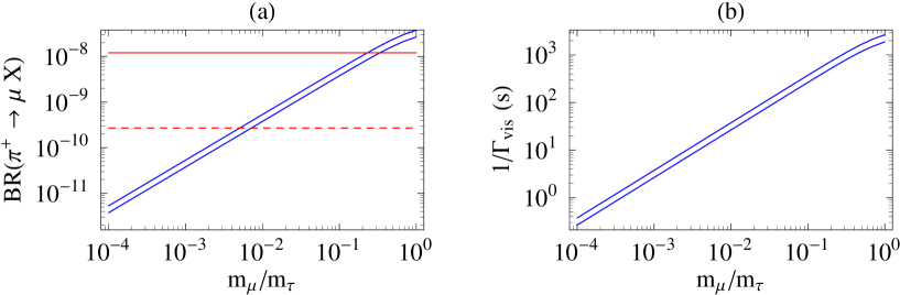
Figure 2: Branching ratio $\text{BR}(\pi^{+}\rightarrow\mu^{+}X)$, (a), and inverse visible width $\Gamma_{\text{vis}}$, (b), as functions of the ratio $r={\hat{m}}_{\mu}/{\hat{m}}_{\tau}$.

Furthermore, a lower constraint on the ${\hat{m}}_{\mu}/{\hat{m}}_{\tau}$ range is given by the requirement that ${\hat{m}}_{\tau}$ is not too large. If ${\hat{m}}_{\tau}$ were of the order of the Dirac mass $\mu$ or more, the $\tau$ neutrino would predominantly consist of a heavy mass eigenstate, which would be phenomenologically problematic. Consequently, $r$ should be preferably in the range

$$r=10^{-4}\;\mbox{to}\;10^{-2}\;.$$ (50)

Then, the mass parameters ${\hat{m}}_{i}$ of our model as well as the branching ratio and the decay width of the $X$ particle can be expressed in terms of $r$ as

$${\hat{m}}_{\mu}=(4.0\,\text{--}\,4.7)\,\mathrm{keV}\left(\frac{r}{10^{-2}}\right)^{1/2}$$ (51a)

$${\hat{m}}_{\tau}=(0.4\,\text{--}\,0.47)\,\mathrm{MeV}\left(\frac{10^{-2}}{r}\right)^{1/2}$$ (51b)

$$\text{BR}(\pi^{+}\rightarrow\mu^{+}X)=(3.8\,\text{--}\,5.3)\,10^{-10}\,\left(\frac{r}{10^{-2}}\right)$$ (51c)

$$\tau_{X}<\Gamma_{\text{vis}}^{-1}=(27\,\text{--}\,38)\,\text{sec}\,\left(\frac{r}{10^{-2}}\right).$$ (51d)

It remains to fix the radius $R$ of the two additional dimensions. Of course, $1/R$ should be smaller than the mass $m_{\rm X}\simeq 33.9\,\mathrm{MeV}$ of the $X$ particle. Furthermore, as we have seen in Section 2, a value of $1/R\simeq 1.6\,\mathrm{MeV}$ leads to a complete solution of the fine–tuning problem. However, as explained there, we need to choose a somewhat larger value $1/R\gtrsim 15\,\mathrm{MeV}$ to avoid significant contributions from modes lighter than the $X$ particle to the KARMEN spectrum. In summary, we therefore require

$$15\,\mathrm{MeV}\lesssim 1/R<33.9\,\mathrm{MeV}\;.$$ (52)

The fine–tuning is smallest at the lower end of this range which is why we have chosen $1/R\simeq 15\,\mathrm{MeV}$ in the fit performed in Section 2. Finally, we have to fix the order of magnitude of our Dirac mass $\mu$. To avoid too large admixture of the lightest Kaluza–Klein mode we have to require that $\mu\gg{\hat{m}}_{\tau}$. In addition, of course, $\mu$ has to be smaller than the $X$ particle mass. Together, this leads to

$${\hat{m}}_{\tau}\ll\mu<33.9\,\mathrm{MeV}\;.$$ (53)

We remark that this allows for the plausible value $\mu=O(1/R)$ for the Dirac mass. Finally, we should check the assumption made in the previous section about the unitarity of the matrix $N$ and the smallness of the heavy states contribution to the SM neutrinos. Both issues are related to the square of the normalization matrix $N^{\dagger}N$ defined in eq. (29) which should be close to unity. For our favorite values $1/R\simeq\mu\simeq 15\,\mathrm{MeV}$ and $M_{\rm s}=1\,\mathrm{TeV}$ this square is given by

$$N^{\dagger}N\simeq 1+0.05\left(\frac{10^{-2}}{r}\right)\;$$ (54)

It constraints $r$ to be in a subset of the range (50) which, however, is still comfortably large.

Now that we have basically fixed all the lepton number conserving quantities in our model we should analyze what we need to do to generate small masses for the neutrinos. In the previous section we have shown that we can generate neutrino masses by introducing a lepton number breaking bulk Majorana mass $M$ and lepton number violating brane–bulk masses $\tilde{m}_{\pm}$. Both mass terms violate lepton number by two units. For the simple case of one neutrino flavor the resulting neutrino mass has been given in eq. (39). Using our favorite values $1/R\simeq\mu\simeq 15\,\mathrm{MeV}$ and ${\hat{m}}_{\pm}\simeq{\hat{m}}_{\tau}$ where ${\hat{m}}_{\tau}$ has been specified in eq. (50) we find

$$m_{0}\simeq\left(\frac{10^{-2}}{r}\right)\left(-2\frac{\tilde{m}_{\tau}}{{\hat{m}}_{\tau}}+\frac{M}{\mu}\right)(1.5\,\text{--}\,2.0)\,\mathrm{MeV}\;.$$ (55)

Note that the two ratios $\tilde{m}_{\tau}/{\hat{m}}_{\tau}$ and $M/\mu$ of lepton number violating and conserving quantities on the brane and in the bulk, respectively, enter with the same strength. This fits nicely to the fact that they both break lepton number by two units. More quantitatively, to have a neutrino mass $m_{0}\lesssim 1\,\mathrm{eV}$ we need both ratios to be less than roughly $10^{-4}r$. Such a number may, for example, arise from a suppression of the form $<\phi>/M_{\rm s}$ where $\phi$ is a boson that carries lepton number and takes a VEV of the order, say $1/R$.

Although the main focus of the paper is on the particle physics aspects of our model, we would like to briefly address constraints from big–bang nucleosynthesis and astrophysics. In the early universe, the Kaluza–Klein mode with mode number $n$ and mixing $U_{in}$ decouples at a temperature of

$$T_{\rm dec,n}\simeq 1\,\mathrm{MeV}|U_{in}|^{-2/3}\;.$$ (56)

From eq. (50) the largest mixing angles are those for $i=\tau$. Using these angles and $\mu=1/R\simeq 15\,\mathrm{MeV}$ as above we find

$$T_{\rm dec,n}\simeq(10\text{--}11)\,\mathrm{MeV}\left(\frac{r}{10^{-2}}\right)^{1/3}(1+n^{2})^{1/3}\;.$$ (57)

It follows than the decoupling temperature is lower than the mass for all Kaluza–Klein modes. In particular, the decoupling temperature increases with a smaller power of the mode number $n$ than the masses $M_{n}\simeq 15\,\mathrm{MeV}\sqrt{1+n^{2}}$ of the Kaluza–Klein modes. As a consequence, modes with large $n$ decouple when they are highly non–relativistic and are strongly diluted. Unfortunately, this suppression is not strong enough for low $n$ modes. Therefore, we have to assume that the bulk is empty at some temperature $T<T_{\rm dec,0}\simeq 10\,\mathrm{MeV}$ as it is customary for models with large additional dimensions [21]. Taking this temperature sufficiently low (but above $1\,\mathrm{MeV}$, of course) recreation of Kaluza–Klein particles is Boltzmann–suppressed. As a consequence, their thermal production rate can always be kept below the Hubble rate.

Supernova cooling provides another constraint on our model. For the single–particle explanation of the KARMEN anomaly the supernova energy loss induced by the $X$ particle has been estimated in ref. [22]. From this estimate, it is concluded there, that the single particle explanation of the KARMEN anomaly is ruled out. Our model is even more problematic since we have a tower of particles rather than just a single one. However, a closer analysis of the supernova energy loss [23] is likely to weaken the bound given in ref. [22]. This together with the assumption of a moderately lower supernova temperature might render our model consistent with the supernova constraint. In any case, we believe that our model is of interest from the viewpoint of particle physics and should be compared with the direct experimental information on neutrino properties.

6 Conclusions

In this paper, we have shown that the KARMEN anomaly can be understood in the context of a six–dimensional brane–world model. The slow particle $X$, responsible for the anomaly, is identified with a specific Kaluza–Klein excitation of a bulk fermion that, from a four–dimensional point of view, appears as a sterile neutrino. We have pointed out that in any interpretation of the KARMEN anomaly based on a single slow particle produced in the $\pi^{+}\rightarrow\mu^{+}X$ decay, the $X$ mass is fine–tuned to the mass difference $m_{\pi}-m_{\mu}$ with an accuracy of order $10^{-4}$. This means that $\delta m_{X}/(m_{\pi}-m_{\mu})\sim 1.8\,10^{-4}$, where $\delta m_{X}=(m_{\pi}-m_{\mu})-m_{X}$. Such a problem can be significantly alleviated, although only partially solved, in the approach we propose, since the $X$ particle is just one of the many excitation of the bulk fermion. It is therefore relatively more probable that one out of the many states has a mass that falls into the critical range.

The phenomenology of the model with respect to the KARMEN experiment depends on the average separation $\Delta m_{\text{KK}}$ between two Kaluza–Klein states at the scale $m_{X}$. In the limit where $\Delta m_{\text{KK}}$ is large, that is $\Delta m_{\text{KK}}=\mathcal{O}\left(m_{\pi}-m_{\mu}\right)$, the model is indistinguishable from models with a single sterile neutrino. In this limit, although the fine–tuning is not improved, we still have a model that provides a theoretically well–motivated origin for the $X$ particle. Moreover, as a quite non–trivial feature, the model allows to incorporate the large mass scale of the $X$ particle as well as the small neutrino masses needed for the standard oscillation phenomenology. The limit of small $\Delta m_{\text{KK}}$, that is $\Delta m_{\text{KK}}=\mathcal{O}\left(\delta m_{X}\right)$, is ruled out because it would lead to a modification of the KARMEN time spectrum in the region $(0.6\,\text{--}\,3.1)\,\mathrm{\mu s}$. For intermediate values of $\Delta m_{\text{KK}}$, $\Delta m_{\text{KK}}=\mathcal{O}\left(1\right)\,\mathrm{MeV}$ or more, the fine–tuning problem is significantly alleviated and the particles lighter than $X$ could give a small contribution to the early KARMEN time spectrum. Therefore, a detailed study of the time distribution of events at early times after the end of the proton pulse could test the model if the mass separation $\Delta m_{\text{KK}}$ happens not to be too large. An upgraded detector with tracking capability devoted to the study of the anomaly could certainly explore this possibility. Needless to say, the detection of a signal at early times would represent a strong hint for the existence of a brane–world.

On the model building side, we have identified two possible structures for the sizes of the additional dimensions. The first case represents an effectively five–dimensional model with intermediate string scale and the remaining five dimensions being close to the string scale. The second one has a $\,\mathrm{TeV}$ string scale, two large dimensions in the $\,\mathrm{MeV}^{-1}$ range and the scale of the remaining four dimensions being two to three orders of magnitude larger. Therefore, in this case the space–time is effectively six–dimensional in an intermediate energy range. We have described in detail a six–dimensional example. As in all brane–world neutrino models, we have considered bulk neutrinos whose Lorenz invariant Dirac and Majorana masses are suppressed relative to the string scale. In particular, we have taken the magnitude of the Dirac mass term to be of the order of the inverse size of the additional dimensions and we have further suppressed the Majorana mass term by means of a U(1) symmetry (lepton number). Despite the introduction of the bulk Dirac mass term, we have found that the model accommodates three light Majorana neutrinos which would be massless in the limit of unbroken U(1) symmetry. The light states are predominantly given by the electroweak eigenstates with small but sizeable admixture of Kaluza–Klein modes. We have therefore attributed the solar and atmospheric neutrino phenomenology to those light states. On the other hand the small heavy component of the flavor eigenstates accounts for the KARMEN anomaly. Therefore, the introduction of the Dirac mass term makes our model rather different from the models considered in the literature so far, where the massless modes either do not exist or decouple from the left–handed neutrinos. Moreover, the neutrino masses and the mixing of neutrinos and bulk states are controlled by different parameters. We believe that such a scheme can be of general interest for brane–world models of neutrino masses.

7 Acknowledgments

We thank Pierre Ramond, Graham Ross and Subir Sarkar for useful discussions and suggestions. This work is supported by the TMR Network under the EEC Contract No. ERBFMRX–CT960090.

References

- [1] P. Horava and E. Witten, “Eleven-Dimensional Supergravity on a Manifold with Boundary,” Nucl. Phys. B475 (1996) 94–114, hep-th/9603142.
- [2] E. Witten, “Strong Coupling Expansion Of Calabi-Yau Compactification,” Nucl. Phys. B471 (1996) 135–158, hep-th/9602070.
- [3] P. Horava, “Gluino condensation in strongly coupled heterotic string theory,” Phys. Rev. D54 (1996) 7561–7569, hep-th/9608019.
- [4] A. Lukas, B. A. Ovrut, K. S. Stelle, and D. Waldram, “The universe as a domain wall,” Phys. Rev. D59 (1999) 086001, hep-th/9803235.
- [5] N. Arkani-Hamed, S. Dimopoulos, and G. Dvali, “The hierarchy problem and new dimensions at a millimeter,” Phys. Lett. B429 (1998) 263, hep-ph/9803315.
- [6] I. Antoniadis, N. Arkani-Hamed, S. Dimopoulos, and G. Dvali, “New dimensions at a millimeter to a Fermi and superstrings at a TeV,” Phys. Lett. B436 (1998) 257, hep-ph/9804398.
- [7] Z. Kakushadze and S. H. H. Tye, “Brane world,” Nucl. Phys. B548 (1999) 180, hep-th/9809147.
- [8] J. D. Lykken, “Weak Scale Superstrings,” Phys. Rev. D54 (1996) 3693–3697, hep-th/9603133.
- [9] K. R. Dienes, E. Dudas, and T. Gherghetta, “Neutrino oscillations without neutrino masses or heavy mass scales: A higher-dimensional seesaw mechanism,” Nucl. Phys. B557 (1999) 25, hep-ph/9811428.
- [10] N. Arkani-Hamed, S. Dimopoulos, G. Dvali, and J. March-Russell, “Neutrino masses from large extra dimensions,” hep-ph/9811448.
- [11] G. Dvali and A. Y. Smirnov, “Probing large extra dimensions with neutrinos,” Nucl. Phys. B563 (1999) 63, hep-ph/9904211.
- [12] R. Barbieri, P. Creminelli, and A. Strumia, “Neutrino oscillations from large extra dimensions,” hep-ph/0002199.
- [13] KARMEN Collaboration, B. Armbruster et al., “Anomaly in the time distribution of neutrinos from a pulsed beam stop source,” Phys. Lett. B348 (1995) 19.
- [14] C. Oehler, “Analysis of the KARMEN time-anomaly.” Proceedings of the 6th conference on Topics in Neutrino and Astro-Particle Physics. See also the KARMEN web page at http://www-ik1.fzk.de/www/karmen/.
- [15] V. Barger, R. J. N. Phillips, and S. Sarkar, “Remarks on the KARMEN anomaly,” Phys. Lett. B352 (1995) 365–371, hep-ph/9503295.
- [16] S. N. Gninenko and N. V. Krasnikov, “Exotic muon decays and the KARMEN anomaly,” Phys. Lett. B434 (1998) 163, hep-ph/9804364.
- [17] J. T. Peltoniemi, “Sterile neutrinos as a solution to all neutrino anomalies,” hep-ph/9506228.
- [18] J. Govaerts, J. Deutsch, and P. M. V. Hove, “Laboratory constraints on a isosinglet neutrino: Status and perspectives,” Phys. Lett. B389 (1996) 700–706, hep-ph/9609201.
- [19] D. Choudhury and S. Sarkar, “A Supersymmetric Resolution of the KARMEN Anomaly,” Phys. Lett. B374 (1996) 87–92, hep-ph/9511357.
- [20] D. Choudhury, H. Dreiner, P. Richardson, and S. Sarkar, “A supersymmetric solution to the KARMEN time anomaly,” hep-ph/9911365.
- [21] N. Arkani-Hamed, S. Dimopoulos, and G. Dvali, “Phenomenology, astrophysics and cosmology of theories with sub-millimeter dimensions and TeV scale quantum gravity,” Phys. Rev. D59 (1999) 086004, hep-ph/9807344.
- [22] A. D. Dolgov, S. H. Hansen, G. Raffelt, and D. V. Semikoz, “Cosmological and astrophysical bounds on a heavy sterile neutrino and the KARMEN anomaly,” hep-ph/0002223.
- [23] S. Sarkar and G. G. Ross, in preparation.