Collision–Induced Decay of Metastable Baby Skyrmions

Many extensions of the standard model predict heavy metastable particles which may be modeled as solitons (skyrmions of the Higgs field), relating their particle number to a winding number. Previous work has shown that the electroweak interactions admit processes in which these solitons decay, violating standard model baryon number. We motivate the hypothesis that baryon–number–violating decay is a generic outcome of collisions between these heavy particles. We do so by exploring a 2+1 dimensional theory which also possesses metastable skyrmions. We use relaxation techniques to determine the size, shape and energy of static solitons in their ground state. These solitons could decay by quantum mechanical tunneling. Classically, they are metastable: only a finite excitation energy is required to induce their decay. We attempt to induce soliton decay in a classical simulation by colliding pairs of solitons. We analyze the collision of solitons with varying inherent stabilities and varying incident velocities and orientations. Our results suggest that winding-number violating decay is a generic outcome of collisions. All that is required is sufficient (not necessarily very large) incident velocity; no fine-tuning of initial conditions is required.

1 Introduction

1.1 Motivation

Many extensions to the standard model which involve strong dynamics at the electroweak scale include new heavy particles which have been modeled as solitons. The simplest model within which such particles can be analyzed is the standard electroweak theory with the Higgs boson mass $m_{H}$ taken to infinity and with a Skyrme term [1] added to the Higgs sector. With these modifications, the Higgs sector supports a classically stable soliton whose mass is of order the weak scale, typically a few TeV.[2]

To understand how solitons arise, note that in the absence of the weak gauge interactions, the Higgs sector of the standard model is a four-component scalar field theory in which a global $O(4)$ symmetry is spontaneously broken to $O(3)$, with vacuum manifold $S^{3}$. In the $m_{H}\rightarrow\infty$ limit, the dynamics is that of an $O(4)$ nonlinear sigma model. Field configurations are maps from three dimensional space onto $S^{3}$, and the solitons (skyrmions) are configurations which carry the associated winding number. The winding number is topological and soliton number is conserved.

Gauging the weak interactions changes the picture qualitatively because the winding number of the Higgs field is not invariant under large gauge transformations. This means that a soliton can either be described as a skyrmion of the Higgs field with gauge field $A_{\mu}=0$ or, equivalently, as a topologically trivial Higgs field configuration with a suitably chosen nonvanishing $A_{\mu}$. The latter description makes manifest the fact that there are sequences of gauge and Higgs field configurations, beginning with a soliton and ending with a vacuum configuration, such that all configurations in the sequence have finite energy. This means that the soliton is only metastable: it is separated from the vacuum only by a finite energy barrier and can decay quantum mechanically by tunneling.[3, 4, 5, 6] Or, the soliton can be kicked over the barrier if it is supplied with energy. The process in which an electroweak soliton is hit with a classical gauge field pulse (a coherent state of $W$-bosons) and caused to decay has been analyzed numerically.[7] It is even possible to find a limiting case of the theory in which the quantum mechanical cross-section for a process in which a soliton is struck by a single $W$-boson and induced to decay can be calculated analytically.[7] In any process in which a soliton is destroyed, one net baryon and one net lepton from each standard model generation is anomalously produced.[7]

Electroweak solitons have also been studied in the electroweak theory with finite Higgs mass, in which the Higgs sector is a linear sigma model.[8] If a Skyrme term is added to the theory, metastable electroweak solitons exist if $m_{H}$ is sufficiently large. In the linear sigma model, the Higgs field can vanish at a point in space with only finite cost in energy. The Higgs winding number is therefore not topological even in the absence of gauge interactions. This means that in a world with gauge interactions and a finite Higgs mass, there are two ways for solitons to decay: either via nontrivial gauge field dynamics, as sketched in the previous paragraph, or via the Higgs field itself simply unwinding.[9]

The metastable electroweak soliton is an intriguing object to study. And yet, it is not found in the standard electroweak theory where the Higgs sector is a linear sigma model with no higher derivative terms. The Higgs sector of the standard model is best thought of as an effective field theory describing the low energy (weak scale) dynamics of the light degrees of freedom in some higher energy theory. The simplest examples of higher energy theories which feature particles which can be described as electroweak solitons in the low energy theory are technicolor theories, in which the technibaryons play this role. Regardless of whether the underlying theory is specifically a technicolor model, it will introduce all higher derivative terms allowed by symmetries, including the Skyrme term, into the Lagrangian of the low energy effective theory. If the Higgs boson is discovered to be light (say, with mass $m_{H}\lesssim v=250$ GeV), the correct low energy effective field theory will almost certainly not support solitons, regardless of the physics of the higher derivative terms. If the Higgs boson is discovered to be heavy, there will be some class of appropriate high energy theories whose low energy effective field theories, although more complicated than that obtained simply by adding a Skyrme term to the standard model, feature metastable electroweak solitons. Discovery of the corresponding TeV scale particles would confirm that nature chooses such a theory.

Processes in which two metastable electroweak solitons collide have to date not been studied. Our purpose in this paper is to use the analysis of a two dimensional toy model which shares some (but not all) of the features outlined above to motivate the hypothesis that the generic outcome of such collisions may be the destruction of one or both solitons. This suggests (but certainly does not demonstrate) that baryon number violation is the generic outcome of collisions between two of the TeV scale particles which can be modeled as solitons.

As a sideline, we note that our numerical methods work equally well for describing soliton–soliton and soliton–antisoliton collisions. Our focus is on soliton decay in soliton–soliton collisions; we note, however, that the numerical simulation of soliton–antisoliton annihilation in the Skyrme model is well-known as a difficult numerical problem, plagued with instabilities. We are able to follow soliton–antisoliton annihilation without difficulty (with energy conserved at the part in $10^{4}$ level). This suggests that our numerical methods — in particular the use of the linear sigma model — may be of broad utility when generalized to 3+1 dimensions.

1.2 Metastable Baby Skyrmions

Let us now introduce the 2+1 dimensional model whose metastable solitons we analyze. The Lagrangian density, which describes the dynamics of a three component scalar field $\vec{\phi}=(\phi^{1},\phi^{2},\phi^{3})$, is

$${\cal L}=F\Biggl{[}\frac{1}{2}\partial_{\alpha}\vec{\phi}\cdot\partial^{\alpha}\vec{\phi} - \frac{\kappa^{2}}{4}(\partial_{\alpha}\vec{\phi}\times\partial_{\beta}\vec{\phi})\cdot(\partial^{\alpha}\vec{\phi}\times\partial^{\beta}\vec{\phi})$$ (1.1)

$$- \mu^{2}(v-\vec{n}\cdot\vec{\phi})-\lambda\left(\vec{\phi}\cdot\vec{\phi}-v^{2}\right)^{2}\Biggr{]}\ .$$

Here, $\vec{n}$ is a unit vector which we choose to be $(0,0,1)$.

To understand the features of this Lagrangian, it is worth beginning by setting $\mu^{2}=0$ and taking the limit $\lambda\rightarrow\infty$. When $\mu^{2}=0$, the theory has an $O(3)$ symmetry. For $\lambda\rightarrow\infty$, one removes the fourth term from (1.1) and instead imposes the constraint that $\vec{\phi}\cdot\vec{\phi}=v^{2}$ at all points in space and time. Because the field $\vec{\phi}$ is constrained to take values on a two-sphere of radius $v$, field configurations with fixed boundary conditions at infinity can be classified by their winding number

$$Q=\frac{1}{8\pi v^{3}}\int{\epsilon_{ab}\vec{\phi}\cdot(\partial_{a}\vec{\phi}\times\partial_{b}\vec{\phi})d^{2}x}=\frac{1}{4\pi v^{3}}\int{\vec{\phi}\cdot(\partial_{x}\vec{\phi}\times\partial_{y}\vec{\phi})\,dx\,dy}\ ,$$ (1.2)

which is integer-valued and topological: configurations with different winding number cannot be continuously deformed into one another. This suggests the possibility of soliton solutions to the classical equations of motion. Solitons in 2+1–dimensional $O(3)$ sigma models were first discussed in Ref. [13], and their quantum field theoretic properties were analyzed in Refs. [14, 15]. Such solitons are often called baby skyrmions [15] because of their similarity to 3+1–dimensional skyrmions. Although our motivation is the analogy to 3+1–dimensional electroweak solitons, we note that baby skyrmions themselves do arise in certain 2+1–dimensional electron systems which exhibit the quantum hall effect [16], although the Lagrangian used in their description differs from that in Eq. (1.1).

The four-derivative term in the Lagrangian (1.1) is the analogue of the Skyrme term. It stabilizes putative solitons against shrinking to arbitrarily small size. If we were working in three spatial dimensions, the two-derivative term would stabilize putative solitons against growing to arbitrarily large size. In two spatial dimensions, however, the two-derivative term cannot play this role because its contribution to the energy of a configuration is scale invariant. We must therefore introduce a zero-derivative term in order to stabilize solitons against growing without bound. Such a term must explicitly break the $O(3)$ symmetry, and therefore has no analogue in 3+1–dimensional electroweak physics, in which no explicit $O(4)$ symmetry breaking terms are allowed. The particular form of the $\mu^{2}$ term in (1.1) therefore has no electroweak motivation; it is analogous to a pion mass term in the 3+1 dimensional Skyrme model, but this is not relevant to us. This model (with $\mu^{2}$ nonzero and $\lambda\rightarrow\infty$) was considered in Ref. [17], and its solitons have been analyzed in detail in Refs. [18, 19]. Similar models, differing only in the choice of the explicit symmetry breaking term in the Lagrangian, have also been analyzed.[20]

The soliton mass and size in the theory with Lagrangian (1.1) with $\lambda=\infty$ are given by[19]

$$M_{\rm sol}=19.47F\left[a_{1}\sqrt{\frac{\kappa\mu}{0.316}}+a_{2}\right]\ ,\ \ \ \ \ \ R_{\rm sol}\sim(3-4)\kappa\sqrt{\frac{0.316}{\kappa\mu}}\ ,$$ (1.3)

with $a_{1}$ and $a_{2}$ dimensionless constants (independent of $\kappa\mu$) satisfying $a_{1}+a_{2}=1$. The parametric dependence of these results can be understood by noting that the energy of a configuration of size $R$ receives contributions of order $FR^{0}$, $F\kappa^{2}R^{-2}$ and $F\mu^{2}R^{2}$ from the first three terms in the Lagrangian (1.1) and that, as described above, a soliton is stabilized by the balance between the four-derivative $\kappa^{2}$ term and the zero-derivative $\mu^{2}$ term.

If we stopped here, with $\lambda$ infinite, our solitons would be absolutely stable, rather than metastable. Soliton–soliton collisions have been simulated in this theory, but of course the solitons never decay.[19] Once $\lambda$ is finite, the fields are allowed to deviate from $\vec{\phi}\cdot\vec{\phi}=v^{2}$, and the soliton configuration with $\vec{\phi}\cdot\vec{\phi}=v^{2}$ found previously in the $\lambda\rightarrow\infty$ theory may unwind and decay. Indeed, we will see that soliton solutions do not exist for $\lambda$ less than some $\lambda_{c}$. If $\lambda>\lambda_{c}$, metastable solitons exist: these solitons are classically stable if left unperturbed, but can be induced to decay if supplied with sufficient energy. Our goal is to determine whether the means by which the energy is delivered is important or whether soliton decay is the result of generic soliton–soliton collisions, without finely tuned initial conditions.

For our purposes, $\lambda$ is the most important parameter in the theory because by choosing its value, we control the energy required to make the soliton decay and indeed control whether solitons exist in the first place. We are not interested in the dependence on the other parameters, and indeed most of them can be scaled away. We first set $v=1$ by rescaling $\phi$. Next, the constant $F$ has units of energy and we henceforth measure energy in units such that $F=1$. Next, $\kappa$ has units of length and we henceforth measure length in units such that $\kappa=1$. Note that this means that $\hbar\neq 1$ in our units, but this will not concern us as we only discuss the classical physics of this model. We have set the speed of light $c=1$ throughout. The parameters $\mu^{-1}$ and $\lambda^{-\frac{1}{2}}$ are also length scales in the Lagrangian, and the theory is therefore fully specified by the two dimensionless parameters $\lambda\kappa^{2}=\lambda$ and $\mu\kappa=\mu$. Although results do depend on $\mu$, we are not interested in this dependence, and we choose to follow Ref. [19] and set $\mu^{2}=0.1$ throughout. Once we have chosen units with $F=\kappa=1$ and have chosen to set $\mu^{2}=0.1$, then $M_{\rm sol}=19.47$ and $R_{\rm sol}\sim(3-4)$ in the theory with $\lambda=\infty$.

In Section 2, we find metastable soliton configurations for finite values of $\lambda$ with $\lambda>\lambda_{c}\sim 7.6$. We shall see that for all values of $\lambda$ for which solitons exist, the soliton mass and size change little from their values at $\lambda\rightarrow\infty$. Although we do not explore their dependence on $\mu$, we expect it would be similar to that in (1.3). In Section 3, we present our results on soliton–soliton collisions. We find that soliton decay occurs for incident velocities greater than some critical value $v_{c}$. We explore how this critical velocity depends on $\lambda$ and on the initial impact parameter and relative orientation of the two solitons. We find that $v_{c}$ is less than or of order half the speed of light regardless of the relative orientation as long as $\lambda\lesssim 2\lambda_{c}$ and $b$ is less than or of order the soliton size. Thus, inducing soliton decay does not require specially chosen initial conditions; it is a generic outcome of soliton–soliton collisions. We make concluding remarks in Section 4.[21]

It perhaps goes without saying that our model is at best a crude toy model for the electroweak physics which motivates our analysis. First, we work in 2+1 dimensions. Second, in order for the theory to have soliton solutions we are forced to include a zero-derivative explicit symmetry breaking term not present in the electroweak theory. Third, we do not introduce a gauge field. Hence, our solitons can only decay via unwinding the scalar field; in the electroweak theory, gauge field dynamics introduces a second decay mechanism which has no analogue in our theory. Related to this, our solitons are absolutely stable for $\lambda=\infty$, whereas electroweak solitons are metastable even for $m_{H}=\infty$. This is perhaps the biggest qualitative difference between our model and electroweak physics. Fourth, one may worry that even if an analysis along the lines of ours were done in the 3+1 dimensional electroweak theory itself, the momenta required would make it impossible to analyze soliton decay within the effective theory. This concern may be evaded for solitons which are almost unstable: in this circumstance, for example, $W$-soliton collisions can result in soliton destruction even if the $W$-boson momentum is small enough that the calculation is controlled.[7] Soliton–soliton scattering in our model is far from being a complete analogue of the scattering of TeV scale particles which can be modeled as metastable electroweak solitons; we nevertheless hope that our central result, namely that metastable baby skyrmions in 2+1 dimensions are destroyed in collisions with generic initial conditions, motivates future work on baryon number violating scattering in this sector.

2 Finding Static Solitons

Before we can study soliton–soliton collisions, we must find the metastable soliton configurations for different values of $\lambda$. We do this by looking for configurations which minimize the static Hamiltonian $H_{\rm static}$ at a given $\lambda$. The static Hamiltonian is given by

$$H_{\rm static}=-\int d^{2}x\,{\cal L}_{\rm static}\ ,$$ (2.4)

where ${\cal L}_{\rm static}$ is the Lagrangian density of (1.1) with all terms containing time derivatives set to zero.

We discretize $H_{\rm static}$ on a square lattice of $125\times 125$ points, with the spatial separation between points given by $\Delta x=0.2$ (in our units in which $\kappa=1$). We discretize the two derivative term in the standard fashion, writing it as a sum over terms like

$$\left[\frac{\phi^{i}(x,y)-\phi^{i}(x-\Delta x,y)}{\Delta x}\right]^{2}\ .$$ (2.5)

The Skyrme term is trickier to handle, because it involves terms like

$$\partial_{x}\phi^{1}\,\partial_{y}\phi^{1}\,\partial_{x}\phi^{2}\,\partial_{y}\phi^{2}\ .$$ (2.6)

We discretize this contribution to the Hamiltonian as a sum over terms like

$$\left(\frac{\phi^{1}(x+\Delta x,y)-\phi^{1}(x-\Delta x,y)}{2\Delta x}\right)\left(\frac{\phi^{1}(x,y+\Delta x)-\phi^{1}(x,y-\Delta x)}{2\Delta x}\right)$$ (2.7)

$$\times\left(\frac{\phi^{2}(x+\Delta x,y)-\phi^{2}(x-\Delta x,y)}{2\Delta x}\right)\left(\frac{\phi^{2}(x,y+\Delta x)-\phi^{2}(x,y-\Delta x)}{2\Delta x}\right)\qquad\quad$$

In this way, we ensure that within each term in the sum over lattice sites, all spatial derivatives are centered at the same point in space. Discretizing the Hamiltonian in this fashion ensures that discretization errors are of order $(\Delta x)^{2}$.

In order to find a soliton, we begin with a guess (which we describe momentarily) for the configuration $\vec{\phi}(x,y)$ and perform a numerical minimization of the static Hamiltonian using the conjugate gradient method of Ref. [22]. (It is important to use a method such as this one, which minimizes a function of $N$ variables using computer memory of order $N$ rather than of order $N^{2}$ since we have an $N=3\times 125\times 125$ dimensional configuration space.) In order to minimize the energy, the conjugate gradient routine needs expressions for the gradient of the energy at any point in our $N$ dimensional configuration space, with respect to each direction in this configuration space. We obtain these expressions by varying the discretized $H_{\rm static}$ with respect to the $\phi^{i}$ at each lattice site. (These expressions will of course also appear as the terms with no time derivatives in the dynamical equations of motion of Section 3.)

For $\lambda\rightarrow\infty$, soliton solutions can be written in the form[17, 18]

$$\vec{\phi}(r,\theta)=\left(\begin{array}[]{c}\sin f(r)\cos\theta\\ \sin f(r)\sin\theta\\ \cos f(r)\end{array}\right)$$ (2.8)

where $f(r)$ satisfies the following conditions:

$$f(0)=\pi,$$ (2.9)

$$\lim_{r\rightarrow\infty}f(r)=0\ .$$ (2.10)

(We define polar coordinates such that the soliton is centered at $r=0$, $\theta=0$ is the positive $y$-axis, and $\theta$ increases in a clockwise direction.) Note that because of the $\mu^{2}$ term in the Lagrangian which breaks the $O(3)$ symmetry, $\vec{\phi}$ must point in the $\phi^{3}$ direction at large $r$. The $O(2)$ symmetry associated with rotations in the $(\phi^{1},\phi^{2})$ plane is not broken in the Lagrangian; in the solution, these rotations are mapped onto rotation in the $(x,y)$ plane about the soliton center. This configuration is thus a two-dimensional analogue of what in three dimensions is called a hedgehog configuration.

In our search for solitons at finite $\lambda$, we therefore begin by choosing a reasonably large $\lambda$, namely $\lambda=15$, and making an initial guess of the form (2.8) with $f(r)=\pi\exp(-r/2)$. We then run the conjugate gradient relaxation algorithm repeatedly, until the change in the energy between successive relaxation steps is smaller than one part in $10^{10}$. The soliton configuration we find is a hedgehog configuration, as at $\lambda\rightarrow\infty$. However, when $\lambda$ is finite, $\vec{\phi}\cdot\vec{\phi}\neq 1$. The soliton we find can be written in the form

$$\vec{\phi}(r,\theta)=\sigma(r)\left(\begin{array}[]{c}\sin f(r)\cos\theta\\ \sin f(r)\sin\theta\\ \cos f(r)\end{array}\right)$$ (2.11)

with $f(r)$ satisfying the same boundary conditions as above. We depict the soliton configuration in Fig. 1.

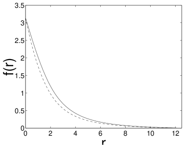
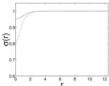
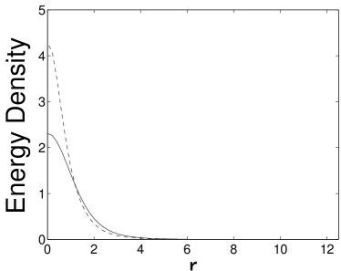
Figure 1: $f(r)$, $\sigma(r)$ and the energy density for the solitons with $\lambda=15$ (solid curves) and $\lambda=7.7$ (dashed curves).

After obtaining a baby skyrmion at $\lambda=15$, we used the resulting configuration as the initial condition for relaxation at $\lambda=14$, and so found the soliton configuration at this $\lambda$. We repeated this process step-by-step in $\lambda$, finding solitons for values of $\lambda$ down to $\lambda=8$. At $\lambda=7$, energy minimization led to a configuration with zero energy, instead of to a soliton. We then used the $\lambda=8$ soliton as an initial configuration for relaxation at $\lambda=7.9$, and so on down to $\lambda=7.6$ where again no soliton was found. We therefore know that a stable soliton exists at $\lambda=7.7$. It is a logical possibility that there is a stable soliton at $\lambda=7.6$ even though our relaxation algorithm did not find one. We think this is unlikely, because the soliton configurations which we have found at $\lambda=7.7$ and $\lambda=7.8$ are very similar, and we therefore believe that the $\lambda=7.7$ soliton is a very good starting configuration from which to find the $\lambda=7.6$ soliton if it existed. We therefore conclude that classically stable solitons exist only for $\lambda>\lambda_{c}$, with $7.6<\lambda_{c}<7.7$.

$\lambda$	Energy
15	19.1792
14	19.1503
13	19.1161
12	19.0751
11	19.0250
10	18.9618
9	18.8791
8	18.7619
7.9	18.7473
7.8	18.7309
7.7	18.7131
7.6	no soliton

Table 1: Energy of Static Solitons at various Lambdas.

In Table I, we give the energies of the solitons which we have found for various values of $\lambda$. In Fig. 1, we depict the field configuration and energy density for the solitons we have obtained for $\lambda=15$ and $\lambda=7.7$. We note that even though $\lambda=7.7$ is only just above $\lambda_{c}$, the soliton configuration does not look very different from that at much larger values of $\lambda$, and the soliton energy is also little changed. Note that the deviation from $\sigma(r)=1$ is only at most $20\%$ for a soliton with $\lambda=7.7$ which is on the edge of instability. The central energy density does increase by almost a factor of two as $\lambda$ is reduced from 15 to 7.7. Note, however, that the total energy is almost unchanged, and actually decreases slightly. The soliton radius decreases as $\lambda$ is reduced towards $\lambda_{c}$, but does not decrease dramatically. The definition of $R_{\rm sol}$ is of course somewhat arbitrary; if we take it to be the radius inside which $90\%$ of the total energy of the soliton is found, we find $R_{\rm sol}=3.31$ for $\lambda=15$ and $R_{\rm sol}=2.83$ for $\lambda=7.7$.

Although the energy density and $\sqrt{\vec{\phi}\cdot\vec{\phi}}=\sigma$ are circularly symmetric, the fields $\phi^{1}$ and $\phi^{2}$ in a soliton configuration are not circularly symmetric. If we only observed a single static soliton, this would be of no consequence: in a hedgehog configuration, the different possible choices for $\phi^{1}$ and $\phi^{2}$ are related simply by rotations in space. However, when we describe a configuration of two well-separated solitons in the next Section, the relative angle $\alpha$ between their orientations does matter. That is, specifying such a configuration requires giving the relative position and velocity of the centers of the two solitons and the angle $\alpha$. The first soliton in such a configuration can be mapped onto the second by a translation followed by a rotation by an angle $\alpha$ about the soliton center.

3 Colliding Solitons

With solitons in hand, we are ready to study what happens when they collide. For this purpose, we need discretized equations of motion and a numerical algorithm to evolve an initial configuration, now specified by $\phi^{i}$ and $\dot{\phi}^{i}$ at each lattice site, forward in time. We begin by writing a discretized Lagrangian which is a function of $\phi^{i}$ and $\dot{\phi}^{i}$ at each of the lattice sites, at a single time $t$. We discretize the time-independent terms as described in the previous Section. There are no spatial derivatives of $\dot{\phi}^{i}$ in the Lagrangian, so discretizing terms involving $\dot{\phi}^{i}$ is trivial. We then use the Euler-Lagrange procedure on this Lagrangian written in terms of $3\times 125\times 125$ $\phi$’s and $3\times 125\times 125$ $\dot{\phi}$’s, and obtain equations of motion which specify the $3\times 125\times 125$ $\ddot{\phi}$’s. These equations of motion take the form of three coupled linear equations for $\ddot{\phi}^{1}$, $\ddot{\phi}^{2}$ and $\ddot{\phi}^{3}$ at a given lattice site, which are easily solved. We now have an expression for $\ddot{\phi}^{i}(t,x,y)$ written in terms of the values of $\phi^{i}$ and $\dot{\phi}^{i}$ at lattice sites within two spatial links of the site of interest, all at the same time $t$. We are now ready to take a step forward in time.

We evolve the system forward in time using the Runge-Kutta-Feldberg algorithm and the adaptive algorithm of Ref. [22] for choosing the size of the time step $\Delta t$. That is, we first use the fifth-order Runge-Kutta-Feldberg algorithm to obtain $\phi^{i}$ and $\dot{\phi}^{i}$ at time $t+\Delta t$. This fifth-order method is special because a rearrangement of the fifth-order function evaluation terms results in a fourth-order Runge-Kutta expression. We then have two different estimates (fourth order and fifth order) for $\phi^{i}$ at $t+\Delta t$ at each lattice site, and can evaluate the discrepancy between the two estimates for each of the $3\times 125\times 125$ $\phi$’s and $\dot{\phi}$’s. If the largest discrepancy is larger than a specified tolerance, we reject the step and begin anew with a smaller $\Delta t$. We use the largest discrepancy to estimate how much $\Delta t$ should be reduced. If all discrepancies are smaller than the specified tolerance, we accept the result of the fifth-order calculation for $\phi^{i}$ and $\dot{\phi}^{i}$ at time $t+\Delta t$. After a successful step forward in time, we use the largest discrepancy (which must have been less than the tolerance since the step forward was accepted) to estimate by how much we can safely increase $\Delta t$ when we take our next step forward in time. In the simulations of collisions which we describe below, the tolerance is such that the timestep selected by the adaptive algorithm is approximately $0.01\lesssim\Delta t\lesssim 0.05$. Note that we do not use conservation of energy as our criterion for acceptance or rejection of a step forward in time. This makes it fair to use a check of the conservation of energy as an independent measure of the accuracy of our evolution algorithm. We do this at various points below.

We choose fixed boundary conditions, with $\vec{\phi}$ fixed to its vacuum value $(0,0,\sigma_{\rm vac})$ at the boundaries of our $125\times 125$ grid, where $\sigma_{\rm vac}$ solves $(\sigma_{\rm vac}^{2}-1)\sigma_{\rm vac}=\frac{\mu^{2}}{4\lambda}$ and is $\sigma_{\rm vac}\simeq 1+\frac{\mu^{2}}{8\lambda}$ for large $\lambda$. Since the solitons have radii of order $R_{\rm sol}\simeq 3$, we choose initial conditions with two solitons whose centers are a distance $10$ apart. We initialize $\vec{\phi}$ by adding these two soliton configurations. (That is, we take $\vec{\phi}_{\rm vacuum}+(\vec{\phi}_{\rm first~{}soliton}-\vec{\phi}_{\rm vacuum})+(\vec{\phi}_{\rm second~{}soliton}-\vec{\phi}_{\rm vacuum})$.) The resulting configuration is not precisely a minimum of the static Hamiltonian, but the two solitons are far enough apart that this is not a big concern. To obtain a soliton moving with an initial speed $v$ in the positive $x$ direction, we simply initialize

$$\dot{\phi}^{i}(x,y)=-v[\phi^{i}(x,y)-\phi^{i}(x-\Delta x,y)]/\Delta x$$ (3.12)

at time zero. For simplicity, we are using a Galilean boost. This is appropriate for $v\ll 1$. When we use this prescription with a velocity at which relativistic corrections are becoming important, the initial condition we have specified is not the correct Lorentz-boosted, Lorentz-contracted soliton. In this circumstance, as the system is evolved forward in time, the soliton radiates some energy and quickly settles down to become a (correct) relativistic soliton moving with a velocity somewhat less than $v$. For example, when we set $v=0.8$ in our Galilean boost prescription for the initial condition, we in fact end up with a soliton moving at a speed of $0.61$.

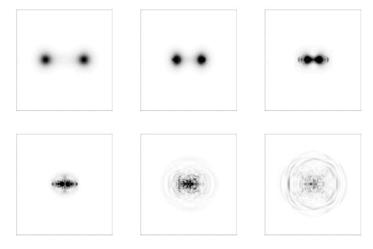
Figure 2: Sequence of snapshots of the energy density during a collision between two solitons which results in the destruction of both. The grey scale indicates energy density. In this simulation, $\lambda=10$, the initial velocity of each soliton is $v=0.5$, the impact parameter is $b=0$, and the solitons have a relative orientation angle $\alpha=0$ in the initial configuration. The images are at times $t=0,4,8,12,16,20$. In this and in all subsequent figures showing soliton–soliton collisions, each panel shows a $25\times 25$ square (in our units in which $\kappa=1$) and the initial separation between solitons is 10. The lattice spacing is $\Delta x=0.2$.

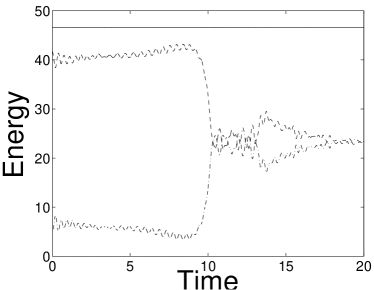
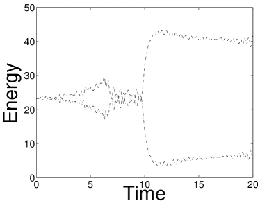
Figure 3: Left panel: Kinetic, potential and total energies during the soliton–soliton collision shown in Fig. 2 with $\lambda=10$ and $v=0.5$. The topmost curve (constant to better than two parts in $10^{5}$) is the total energy. Of the other two curves, the one that begins low is the kinetic energy, the one that begins high is the potential energy, including spatial gradient energy. Right panel: Same, during the time–reversed evolution. We reverse the sign of all $\dot{\phi}^{i}$ in the final configuration of Fig. 2, and then watch the evolution algorithm recreate the initial configuration of Fig. 2.

We begin by analyzing collisions between two solitons in the theory with $\lambda=10$. We choose initial conditions in which both solitons are moving (towards each other) with velocity $v=0.25$, with zero impact parameter. We choose an initial relative orientation angle $\alpha=0$, meaning that one soliton is obtained from the other by translation without rotation. Previous work shows that two static solitons with this relative orientation repel each other.[19] This is consistent with what we find: for low velocities, as for example for $v=0.25$, the two solitons bounce off each other and return whence they came. We now increase $v$ to $0.5$. This time, the outcome, depicted in Fig. 2, is that the solitons are destroyed in the collision. The final state is a cloud of debris, namely small amplitude oscillations of the $\vec{\phi}$ field spreading outwards from the scene of the collision. In Fig. 3, we show the kinetic energy, potential energy and total energy for the collision shown in Fig. 2. (By “potential energy” we mean the contribution to the energy from all those terms in the Hamiltonian with no time derivatives. Most of this energy is due to spatial gradients of the fields.) First, we see that the total energy is conserved, in fact to better than two parts in $10^{5}$. The kinetic energy is not zero initially, because the solitons are moving. As the solitons approach each other, the kinetic energy decreases. This confirms that the interaction is repulsive: the solitons slow down and deform as they approach. As the solitons approach each other more closely, at some point their deformation becomes sufficient that they are no longer stable, and they fall apart. The resulting outgoing waves have approximately equal kinetic and potential energy, as expected for traveling waves. It is quite clear from Fig. 3, if it was not already clear from Fig. 2, that the solitons have been destroyed.

As a stringent check of the accuracy of our time evolution algorithm, we take the final configuration from our simulation, reverse the sign of $\dot{\phi}^{i}$, and evolve it for the same period of time as we did initially. The second panel of Fig. 3 shows the behavior of the energies during this “backwards-in-time” evolution. It is clear that the debris reconstitutes itself into two solitons! The sequence of snapshots of the energy density looks almost exactly like those in Fig. 2, but in the opposite order in time. The discrepancies between the energy density in the initial configuration and that in the configuration obtained after soliton collision and destruction followed by time-reversed evolution and soliton recreation differ by at most $1/40$ of the energy density at the center of the soliton. The total energy is conserved to better than one part in $10^{4}$.

As a further check of the stability of our algorithm, we have also simulated soliton–antisoliton annihilation. We obtain an antisoliton configuration from a soliton configuration by making the transformation $\phi^{2}\rightarrow-\phi^{2}$, equivalent to taking $\theta\rightarrow-\theta$ in (2.8) or (2.11). This turns a hedgehog configuration into an anti-hedgehog configuration, and hence yields an antisoliton. We find that analyzing soliton–antisoliton collisions using our evolution algorithm is no more difficult than analyzing soliton–soliton collisions. We were able to follow the annihilation process with energy conserved to better than one part in $10^{4}$. Now, with confidence in the accuracy and stability of our evolution algorithm, we proceed to analyze the outcome of soliton–soliton collisions with a variety of initial conditions.

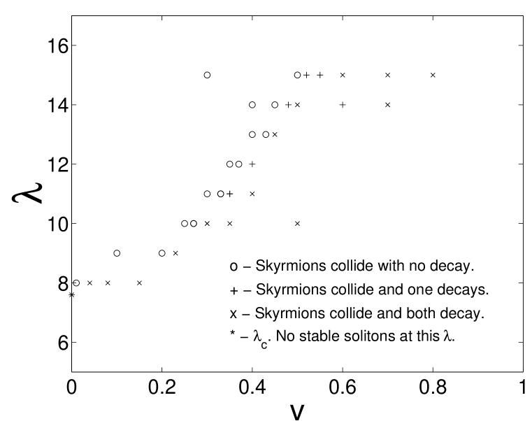
Figure 4: Outcome of soliton–soliton collisions with different initial velocities and different values of the parameter $\lambda$. All collisions have impact parameter $b=0$ and relative orientation angle $\alpha=0$. Note that $v$ is the velocity parameter in (3.12). If $v$ is large enough that relativistic effects are significant, the actual velocity of the soliton is somewhat less than $v$. For example, $v=0.8$ yields a soliton with velocity $0.61$.

We first explore how the outcome of a collision depends on $\lambda$ and $v$, keeping the impact parameter $b=0$ and the relative orientation angle $\alpha=0$ as above. The results of many simulations are summarized in Fig. 4. We discover that for any $\lambda$, there is a critical velocity $v_{c}$ below which the solitons rebound without decaying, and above which one or both (usually both) solitons are destroyed. This critical velocity goes to zero as $\lambda\rightarrow\lambda_{c}$. As $\lambda$ is increased, $v_{c}$ increases, reaching about half the speed of light for $\lambda$ about twice $\lambda_{c}$

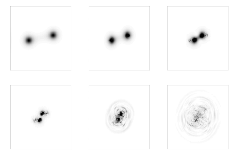
Figure 5: Snapshots of energy density during a collision between two solitons with impact parameter $b=2.0$ in the theory with $\lambda=10$. The relative orientation angle is $\alpha=0$. The initial velocity $v=0.5$ is large enough that the solitons are destroyed. The time between images is $4.0$.

We now return to $\lambda=10$, $v=0.5$, still keeping $\alpha=0$ and ask how the outcome of a collision depends on the impact parameter $b$. For $b=2.0$, both solitons decayed into traveling waves, as we found for $b=0$ above. We show the outcome of this collision in Fig. 5. Note that $b=2.0$ is a substantial impact parameter, comparable to the soliton radius $R_{sol}\simeq 3$. We find that the solitons still decay if $b=3.2$. An impact parameter $b=4.0$, however, yields a collision which is sufficiently peripheral that the solitons emerge intact, deflected from their initial directions of motion by about $45^{\circ}$. We can describe our results by saying that the critical velocity $v_{c}$ above which soliton decay is the outcome of the collision increases with increasing impact parameter. For $b=0$, Fig. 4 shows that $0.27<v_{c}<0.3$. We now see that $v_{c}=0.5$ for a nonzero impact parameter in the range $3.2<b<4.0$. We have also done several more simulations with $b=2.0$ and various initial velocities, and find that for $b=2.0$, the critical velocity is $0.3<v_{c}<0.4$. We conclude that soliton decay does not require collisions with small or finely-tuned impact parameters. Although increasing $b$ from zero increases the critical velocity $v_{c}$ required to destroy the solitons somewhat, it remains easy to destroy solitons as long as the impact parameter is less than or comparable to the soliton radius.

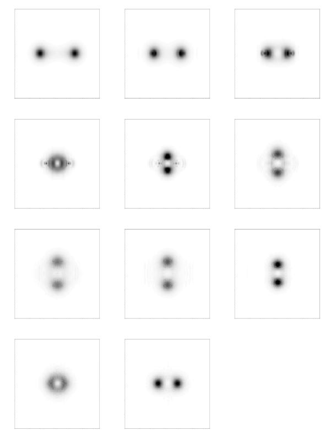
Figure 6: Snapshots of energy density during a collision between solitons with relative orientation $\alpha=180^{\circ}$, impact parameter $b=0$, and initial velocity $v=0.25$ in the theory with $\lambda=10$. The solitons are not destroyed and (eventually) form a classically stable bound state. The time interval between images varies: the images are at times $t=0,4,8,12,16,20,24,28,34,42,50$.

All the collisions we have described to this point have had the same relative orientation. For $\alpha=0$, low velocity collisions yield a rebound, in which each soliton reverses direction, while higher velocity collisions lead to soliton destruction. We now consider a collision (with $\lambda=10$, $v=0.25$ and $b=0$) between two solitons with a relative orientation angle $\alpha=180^{\circ}$. That is, the second soliton in the initial configuration is obtainable from the first by a translation and a $180^{\circ}$ rotation. The interaction between static solitons with this orientation is known to be attractive.[19] We show the outcome of a low velocity collision in Fig. 6. The work of Ref. [18] reveals that in the $\lambda\rightarrow\infty$ theory, there is a stable, ring-shaped, soliton with winding number 2. It appears that the final state of the collision in Fig. 6 will be a soliton of this form, although it will differ in its details from that of Ref. [18] since $\lambda$ is finite. What we observe in Fig. 6 is that the incident solitons at first scatter by $90^{\circ}$, but then do not escape to infinity. They fall back upon one another, and rescatter by $90^{\circ}$. There are small outgoing ripples at late time, but they have too little energy density to be visible in Fig. 6. We expect that were we to run the simulation for a long time, in a big enough box that outgoing ripples never return, we would see repeated $90^{\circ}$ scatterings, with the solitons escaping less and less far away each time, all the while radiating small outgoing ripples, and eventually settling down to become the static, ring-shaped configuration.

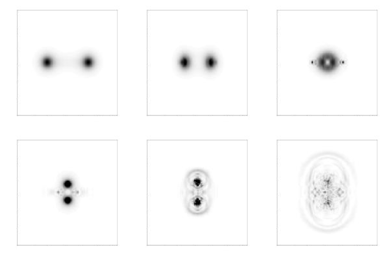
Figure 7: Snapshots of energy density during a collision between two solitons with relative orientation $\alpha=180^{\circ}$ in the theory with $\lambda=10$. The impact parameter is $b=0$. The initial velocity is large enough ($v=0.5$) that the two solitons decay. The time between each image is $4.0$.

As we increase the incident velocity, we find that for $v>v_{c}$ with $0.43<v_{c}<0.48$, the outcome of the collision is soliton destruction rather than $90^{\circ}$ degree scattering followed by the formation of a bound state. We show an example of collision induced decay in a collision with relative orientation $\alpha=180^{\circ}$ in Fig. 7. Note that the critical velocity above which soliton destruction is the outcome is somewhat larger than, but still comparable to, that we found previously for $\alpha=0$. We have not mapped out $v_{c}$ vs. $\lambda$ for the $\alpha=180^{\circ}$ orientation as we did in Fig. 4, but we expect that the figure would be qualitatively similar. One new feature, though, would be that at large $\lambda$ there would be two different outcomes possible for collisions with $v<v_{c}$: bound state formation (for low enough $v$) and $90^{\circ}$ scattering followed by the escape of the two intact solitons to infinity (for larger $v$ which is still less than $v_{c}$). At $\lambda=10$, we do not find any velocities for which $90^{\circ}$ scattering followed by escape occurs. It must occur at larger $\lambda$, since it certainly occurs at large enough velocities for $\lambda\rightarrow\infty$, when $v_{c}\rightarrow 1$.

The collision shown in Fig. 7 is an example of a simulation in which the initial velocity ($v=0.5$ in this case) is only just above the critical velocity ($0.43<v_{c}<0.48$ in this case). In this circumstance, what we generically observe is that the solitons scatter, separate a little, but are sufficiently distorted as a result of the scattering that after separating a little they fall apart. We observe this phenomenon also at $\alpha=0$, except in this case the solitons scatter by bouncing back in the direction whence they came, then separate a little, and then fall apart. At velocities which are somewhat larger than $v_{c}$, as for example in the collision shown in Fig. 2, we find that soliton destruction occurs more promptly, during the initial collision.

We now consider collisions between solitons with a relative orientation angle $\alpha=90^{\circ}$, still with $\lambda=10$ and $b=0$. For this relative orientation, there is no force between static solitons.[19] We find the same possible outcomes as we did for $\alpha=180^{\circ}$. As a function of increasing velocity, the outcome of a collision is either capture to form the ring-shaped bound state, or soliton destruction. (Again, scattering by an angle of $90^{\circ}$ followed by the escape of two intact solitons would be a possibility at larger $\lambda$.) The critical velocity above which soliton decay occurs is $0.25<v_{c}<0.3$.

4 Concluding Remarks

We have analyzed soliton–soliton collisions in a $2+1$-dimensional theory with metastable baby skyrmion solutions. We find classically stable soliton solutions for values of the parameter $\lambda$ which are larger than $\lambda_{c}\sim 7.6$. These solitons are prevented from decaying by a finite energy barrier and so can decay if supplied with sufficient energy, for example in a collision with a second soliton. We have mapped out the space of initial conditions under which the outcome of a soliton–soliton collision is the destruction of one or both solitons. We find that soliton decay results whenever two solitons collide with an incident velocity greater than some $v_{c}$. This critical velocity depends on the parameters in the problem. It goes to zero as $\lambda\rightarrow 0$ and the solitons cease to be classically stable. It goes to the speed of light as $\lambda\rightarrow\infty$ and the barrier to decay becomes infinite. However, $v_{c}$ does not rise particularly rapidly with $\lambda$: with other parameters chosen as in Fig. 4, $v_{c}$ is only half the speed of light for $\lambda\sim 2\lambda_{c}$. Thus, soliton destruction does not require that the theory have a value of $\lambda$ lying in some narrow range just above $\lambda_{c}$. The impact parameter $b$ need not be finely tuned either. Not surprisingly, $v_{c}$ is lowest for collisions with $b=0$. However, $v_{c}$ increases by less than a factor of two for $b$ of order the soliton radius. $v_{c}$ also depends on the relative orientation angle $\alpha$ between the two solitons in the initial state. Here too, the dependence is weak. In the example we explored in detail, we found that as $\alpha$ changes from $0^{\circ}$ to $180^{\circ}$, $v_{c}$ varies between $0.25<v_{c}<0.3$ and $0.43<v_{c}<0.48$. Thus, although $v_{c}$ does depend on $\lambda$ and on the parameters other than the velocity needed to fully specify a choice of initial conditions, the variation of $v_{c}$ is not dramatic. Soliton decay is not restricted to specially chosen velocities, impact parameters, orientations, or values of $\lambda$. Soliton decay is a generic outcome of soliton–soliton collisions.

Our findings motivate future investigation of collisions between metastable solitons in the $3+1$-dimensional electroweak theory. Previous work on two-particle collisions involving these electroweak solitons has focussed on collisions between a $W$ boson and a soliton [7]. In such collisions, the probability for soliton decay falls exponentially as the (rough) analogue of $\lambda$ is increased above the (rough) analogue of $\lambda_{c}$. This was traced to two facts: First, causing one of these solitons to decay requires delivering sufficient energy to one particular mode of oscillation of the soliton. Second, a generic incident $W$-boson couples very weakly to the mode which must be energized if decay is to be induced. We find no analogue of this difficulty in our analysis of soliton–soliton collisions in $2+1$ dimensions. If there is a particular mode which must be excited, then soliton–soliton collisions seem to generically deliver energy to this mode. And, we certainly see no evidence of soliton decay being restricted to theories with $|\lambda-\lambda_{c}|\ll\lambda_{c}$. This suggests that collisions between two TeV scale particles which can be modeled as electroweak solitons (rather than between one $W$-boson and one such particle) may be an arena in which two-particle collisions generically lead to baryon number violation. As we stressed in the Introduction, however, the metastable baby skyrmions we analyze differ in several important qualitative respects from metastable electroweak solitons. Furthermore, our analysis has been purely classical whereas the analysis of $W$-soliton collisions in Ref. [7] is quantum mechanical. Although our results motivate an analysis of collisions between electroweak solitons, they should not be taken to provide even qualitative guidance as to the outcome of such a study.

Acknowledgements

We thank S. Bashinsky, M. A. Halasz, J. Leffingwell, A. Lue, B. Scarlet and S. Sondhi for very helpful discussions. KR is grateful to the Department of Energy’s Institute for Nuclear Theory at the University of Washington for generous hospitality and support during the completion of this work. The work of KR is also supported in part by the Department of Energy under cooperative research agreement DF-FC02-94ER40818, by a DOE OJI Award and by the Alfred P. Sloan Foundation.

References

- [1] T. H. R. Skyrme, Proc. R. Soc. London A260, 127 (1961).
- [2] J. M. Gipson and H. C. Tze, Nucl. Phys. B183, 524 (1981); J. M. Gipson, ibid. B231, 365 (1984).
- [3] E. D’Hoker and E. Farhi, Phys. Lett. 134B, 86 (1984); Nucl. Phys. B241, 109 (1984).
- [4] J. Ambjorn and V. A. Rubakov, Nucl. Phys. B256, 434 (1985); V. A. Rubakov, ibid B256, 509 (1985).
- [5] V. A. Rubakov, B. E. Stern and P. G. Tinyakov, Phys. Lett. B160, 292 (1985).
- [6] G. Eilam, D. Klabucar and A. Stern, Phys. Rev. Lett. 56, 1331 (1986); G. Eilam and A. Stern, Nucl. Phys. B294, 775 (1987).
- [7] E. Farhi, J. Goldstone, A. Lue and K. Rajagopal, Phys. Rev. D 54, 5336 (1996) [hep-ph/9511219].
- [8] J. Baacke, G. Eilam and H. Lange, Phys. Lett. B199, 234 (1987); L. Carson, proceedings of Beyond the Standard Model II, Norman, OK, 224 (1990).
- [9] A. Lue and M. Trodden, Phys. Rev. D58, 057901 (1998) [hep-ph/9802281].
- [10] J. J. Verbaarschot, T. S. Walhout, J. Wambach and H. W. Wyld, Nucl. Phys. A461, 603 (1987); A. E. Allder, S. E. Koonin, R. Seki and H. M. Sommermann, Phys. Rev. Lett. 59, 2836 (1987); H. M. Sommermann, R. Seki, S. Larson and S. E. Koonin, Phys. Rev. D 45 4303 (1992).
- [11] W. Y. Crutchfield and J. B. Bell, J. Comp. Phys. 110, 234 (1994).
- [12] R. D. Amado, M. A. Halasz and P. Protopapas, Phys. Rev. D61, 074022 (2000) [hep-ph/9909426].
- [13] A. A. Belavin and A. M. Polyakov, JETP Lett. 22, 245 (1975).
- [14] F. Wilczek and A. Zee, Phys. Rev. Lett. 51, 2250 (1983).
- [15] R. Mackenzie and F. Wilczek, Int. J. Mod. Phys. A3, 2827 (1988).
- [16] S. L. Sondhi, A. Karlhede, S. A. Kivelson and E. H. Rezayi, Phys. Rev. B 47, 16419 (1993).
- [17] B. M. Piette, W. J. Zakrzewski, H. J. Mueller-Kirsten and D. H. Tchrakian, Phys. Lett. B320, 294 (1994).
- [18] B. M. Piette, B. J. Schroers and W. J. Zakrzewski, Z. Phys. C65, 165 (1995) [hep-th/9406160].
- [19] B. M. Piette, B. J. Schroers and W. J. Zakrzewski, Nucl. Phys. B439, 205 (1995) [hep-ph/9410256].
- [20] R. A. Leese, M. Peyrard and W. J. Zakrzewski, Nonlinearity 3, 773 (1990); M. Peyrard, B. Piette and W. J. Zakrzewski, Nonlinearity 5, 563 (1992); Nonlinearity 5, 585 (1992); A. Kudryavtsev, B. M. Piette and W. J. Zakrzewski, hep-th/9709187; T. Weidig, hep-th/9811238; P. Eslami, W. J. Zakrzewski and M. Sarbishaei, hep-th/0001153.
- [21] Further results and more detailed descriptions of our method of discretization and of the relaxation and time evolution algorithms may be found in: D. Dwyer, MIT Senior Thesis, unpublished, (2000).
- [22] W. H. Press, S. A. Teukolsky, W. T. Vetterling and B. P. Flannery, Numerical Recipes in C, Cambridge University Press, 1997.