ETH-TH/2000-06

April 1999

     BREAD AND BUTTER STANDARD MODEL

Z. Kunszt

Theoretical Physics, ETH Zürich, Switzerland

 Contents:

• Structure of the Standard Model

  • Basic QCD

  • Basic Electroweak Theory
    

• Precision calculations

  • Testing QCD

  • Testing the Electroweak Theory
    

• Higgs sector, Higgs search

  • Difficulties with the Higgs sector

  • Higgs search at LHC

  Lectures given at International School of Subnuclear Physics: 37th Course: Basics and Highlights of Fundamental Physics, Erice, Italy, 29 Aug - 7 Sep 1999.

1 STRUCTURE OF THE STANDARD MODEL

The Standard Model is our theory for the quantitative descriptions of all interactions of fundamental particles except quantum gravity effects. It is highly successful: all measurements are in agreement with the Standard Model predictions.

The Standard Model is a renormalizable relativistic quantum field theory based on non-Abelian gauge symmetry [2] of the gauge group ${SU(3)_{C}\times SU(2)_{L}\times U(1)_{Y}}$. It has two sectors: Quantum Chromodynamics (QCD) and the Electroweak Theory (EW). QCD is a vector gauge theory which describes the $SU(3)_{C}$ color interactions of quarks and gluons. It has rich dynamical structure such as chiral symmetry breaking, asymptotic freedom, quark confinement, topologically non-trivial configurations (monopoles, instantons). The Electroweak Theory (EW) describes the electromagnetic and weak interactions of the quarks and leptons as a chiral non-Abelian isospin and an Abelian hypercharge gauge symmetry $SU(2)_{L}\times U(1)_{Y}$. As a result of the Higgs mechanism, the gauge bosons $W^{\pm},Z$ become massive while the photon remains massless. The true dynamics behind the Higgs mechanism is not yet known. The simple one doublet Higgs sector predicts the existence of a single Higgs boson with well defined properties and its experimental search has first priority. Quarks carry both color and electroweak charges. Quarks and leptons cooperate to cancel the weak gauge anomalies. The Lagrangian of the Standard Model has important accidental global symmetries leading to baryon number and individual lepton number conservation in all orders of perturbation theory without implying absolute conservation of these quantum numbers.

1.1 Basic QCD

In the sixties and early seventies an exciting series of beautiful experiments with many puzzling and unexpected results have lead to the discovery of QCD.

1.1.1 Quarks, flavor, color

Spin 1/2 quarks as elementary constituents of strongly interacting hadrons have been invented by Gell-Mann and Zweig in 1964 to explain the approximate SU(3) spectral symmetry of baryons and mesons. They come in three flavor (up, down and strange) and form the fundamental triplet representation of the approximate SU(3) symmetry. The bound state wave functions of the spin 3/2 baryons decouplet composed from such objects, however, did not follow the Fermi-Dirac statistics. Color was invented by Greenberg in 1964 to restore the validity of the correct spin-statistics, requiring that every quark with a given flavor comes in three colors (red, blue, yellow). The measured normalization of the decay rate $\Gamma(\pi^{0}\rightarrow 2\gamma)$ and of the cross-section $\sigma(e^{+}e^{-}\rightarrow{\rm hadrons})$ dramatically confirmed this assumption. The low lying hadron spectrum also had a more delicate chiral $SU(3)_{L}\times SU(3)_{R}$ symmetry that was broken spontaneously and explicitly and was described in terms of algebra of currents. The nature of the color interactions was not clear. For example, motivated by the success of current algebra, Gell-Mann suggested that the underlying field theory of strong interactions is a quark-gluon theory with one Abelian colorless gluon. Nambu instead assumed that the gluons form the octet representation of the color group $SU(3)_{C}$.

These qualitative physical concepts, however, could not yet be summarized into a consistent quantitative theory. As next development, the quark constituent picture got confirmed by deep inelastic electron and neutrino experiments. The results have naturally been interpreted as the backward scattering of electrons and neutrinos on free pointlike constituents of the proton (parton model). Their quantum numbers could be extracted from the data and it turned out that the partons are quarks invented to explain hadron spectroscopy. The final theory could not be formulated since the parton model was based on the assumption of having approximately free point like constituents at short distances within the bound state wave function. This was “not consistent with the known class of renormalizable field theories” (Feynman) [3].

1.1.2 Breakthrough by ’t Hooft

The breakthrough was achieved by ’t Hooft in 1971 by proving that non-Abelian gauge theories are renormalized: a new class of field theories have been discovered with strikingly new properties. The quantization of non-Abelian gauge theories is far more complex than the well-known case of Quantum Electrodynamics (QED) because of the self-interaction of the gauge field. The algebraic complexity of the Feynman rules as well as the Ward-identities of the exact gauge symmetry made the study very difficult. These theories, however, were considered by many people as irrelevant (non-physical) because the gauge bosons are necessarily massless. ’t Hooft’s proofs of the renormalizability of massless non-Abelian gauge theories [4] and of massive gauge theories [5] with Higgs-mechanism opened the possibility to find the fundamental theory of strong interactions as well as the electroweak interactions.

1.1.3 Towards QCD

The discovery of the renormalizability of Yang-Mills theory by ’t Hooft helped the model builders to put together the concepts of quarks, color and flavor as the basic ingredients of a non-Abelian field theory called Quantum Chromodynamics. Gell-Mann et al. [6, 7] pointed out that if the previously suggested quark-gluon model of strong interactions is modified by replacing the Abelian colorless gluon with a non-Abelian colored gluon sector with exact $SU(3)_{C}$ gauge symmetry, one obtains better agreement with the experimentally established qualitative features of strong interactions. They have also speculated that in these theories quarks and gluons might be permanently confined (quark confinement), chiral symmetry breaking could take place and the so called $U(1)_{A}$ problem may be solved. In addition, a completely new fundamental property of Yang-Mills theories was discovered: at shorter and shorter distances the physics looks the same but the interaction of the particles are reduced [8, 9, 10]. In contrary to the old type of field theories, Yang-Mills theories are well defined at short distances. A field theory is asymptotically free if and only if it is a non-Abelian gauge theory. In addition, the importance of asymptotic freedom in connection with Bjorken scaling was also realized and the possibility to use perturbative methods to calculate strong interaction effects has been pointed out. Gross and Wilczek using Wilson’s operator product expansion and renormalization group method have shown that the short and long distance contributions can be factorized and the short distance part can be consistently described using perturbation theory [11]. They have derived the parton picture and interpreted Bjorken-scaling of deep inelastic scattering as leading order absorption of the virtual photon by free quarks inside the proton. As they could evaluate the corrections in first order, the predictions got spectacularly confirmed by a long experimental effort. By reformulating these results in terms of Feynman diagrams, the so called QCD improved parton model has been established. It provides us a well-defined algorithm for calculating cross-sections of hard scattering processes involving hadrons precisely. In particular, jet, W, Z and heavy quark production have been predicted and properties of bound states involving heavy quarks could be calculated. The discovery of heavy particles offered new experimental possibilities to test the QCD improved parton model predictions.

1.1.4 Confinement

Asymptotic freedom implies that at long distances the color interactions are strong. The system condenses in some way. Quarks and gluons may get permanently confined within the hadronic bound states such that massless gauge-bosons do not appear in the particle spectrum. Wilson has pointed out that quark-confinement is a direct consequence of local gauge symmetry in the (non-physical) strong coupling limit when QCD is formulated on a four dimensional Euclidean lattice [12]. It has been suggested that color neutralization is energetically favored in comparison with color separation. It is generally accepted by now that the mechanism of color confinement is due to the condensation of magnetic monopoles suggested by ’t Hooft [13]. The vacuum of color dynamics is a dual superconductor where instead of condensate of Cooper-pairs one has the condensate of magnetic monopoles. The best formulation of the non-perturbative domain of gluon dynamics is the lattice gauge theory and ’t Hooft’s mechanism of quark confinement has been supported by the results of a number of numerical simulation work [14].

1.1.5 Extended objects, topologically non-trivial gauge configurations

By studying extended objects we can get information on the non-perturbative aspects of the theory. They are interpreted as particles with masses inversely proportional to the coupling constant (’t Hooft-Polyakov magnetic monopoles [15, 16]). Extended solutions of the classical field equations in Euclidean space (instantons) can produce tunneling effects with amplitude depending exponentially on the inverse of the coupling constant [17]. In QCD, instantons are important for breaking the global flavor $U(1)_{A}$ symmetry and providing strong CP-violation effects ($\theta$-term).

1.1.6 The Lagrangian of QCD [18]

The transformation matrix of the fundamental representation of the local $SU(3)$ gauge group is

$$\Omega(x)_{ab}=\left(e^{iT^{A}\xi^{A}(x)}\right)_{ab}\,,\quad T^{A}=\frac{1}{2}\lambda^{A}$$ (1)

where $\lambda^{A}$ denotes the $SU(3)$ Gell-Mann matrices and $\xi^{A}(x)$ is the group parameter $A=1,\ldots 8$ and $a,b=1,2,3$. The Dirac spinor of the quarks transforms like

$$q^{\prime}_{a}(x)=\Omega(x)_{ab}q_{b}(x)$$ (2)

while the gauge (gluon) fields transform inhomogenously

$$T^{C}G^{C}(x)=\Omega(x)T^{C}G^{C}(x)\Omega^{-1}+\frac{i}{g_{s}}\left(\partial_{\mu}\Omega(x)\right)\Omega^{-1}(x)$$ (3)

After the choice of the matter field, renormalizability and gauge symmetry dictates uniquely the form of the classical Lagrangian. Introducing the non-Abelian field strength

$$G^{A}_{\mu\nu} = \partial_{\mu}G^{A}_{\nu}-\partial_{\nu}G^{A}_{\mu}-g_{s}f^{ABC}G^{B}_{\mu}G^{C}_{\nu}$$ (4)

$$D_{ab}^{\mu} = \delta_{ab}\partial^{\mu}+ig_{S}T^{C}_{ab}G^{\mu C}$$ (5)

where $f^{ABC}$ is the structure constant of the $SU(3)$ Lie algebra, one gets

$${\cal L}_{\rm classical} = -\frac{1}{4}G^{A}_{\mu\nu}G_{A}^{\mu\nu}+\sum_{f}\overline{q}^{fa}(x)i\gamma_{\mu}D^{\mu}_{ab}q(x)^{f}_{b}$$

$$-\sum_{f}m_{f}\overline{q}^{fa}(x)q(x)_{fa}\,,\quad f=u,d,\ldots,t$$

where the spinor label are suppressed. Mass terms are allowed since QCD is a vector theory: the color properties of the left and right handed quarks are the same. Renormalizability and gauge invariance, however, allows to add an additional term in the Lagrangian

$${\cal L}_{\theta}=\frac{\theta g_{s}^{2}}{32\pi^{2}}G^{A}_{\mu\nu}\tilde{G}_{A}^{\mu\nu}\,,\quad\tilde{G}_{A}^{\mu\nu}=\frac{1}{2}\epsilon^{\mu\nu\lambda\rho}G^{A,\lambda\rho}\,.$$ (7)

This term can be written as a total derivative of a non-gauge invariant vector field $K_{\mu}$, composed from the gauge field $G_{A}^{\mu}$ and, therefore it can be dropped in the context of the perturbation theory. ${\cal L}_{\theta}$, however, can not be neglected in general. The vector field $K_{\mu}$ is not gauge invariant, it can have singular behavior at infinity and those non-trivial topological field configurations of the QCD vacuum can lead to physical CP-violating effects. But strong CP-violation is severely constrained by the data. One such effect would be the observation of electric dipole moment of the neutron. Using the experimental upper limit one gets $\theta<10^{-9}$. It is puzzling why this term is so small. This question is referred to in literature as the strong CP-problem and its resolution leads to the suggestion of the existence of axions [19].

The classical Lagrangian upon quantization gets modified: the perturbative treatment requires that gauge fixing terms, Fadeev-Popov ghost terms are added to the Lagrangian and renormalization requires counter terms

$${\cal L}={\cal L}_{\rm classical}+{\cal L}_{\rm gauge-fixing}+{\cal L}_{\rm ghost}+{\cal L}_{\rm counter\ terms}\,.$$ (8)

This Lagrangian then uniquely defines the algorithm (Feynman rules) for calculating finite physical amplitudes in perturbative expansion [20]. The quadratic terms give the propagators, the trilinear and quartic terms give the vertices. The form of the counter terms depends on the choice of regularization and renormalization scheme and are obtained by calculating a few ultraviolet divergent self-energy and vertex contribution. The algorithm is particularly simple in the case of dimensional regularization, supplemented by the mass independent $\overline{\rm MS}$ renormalization scheme [21]. The Feynman rules and the one loop counter terms can be found in many textbooks [18].

1.1.7 Running coupling ${\alpha_{S}}(\mu)$ and the $\Lambda$ parameter

From the explicit form of the one loop counter terms one can easily derive the leading term of the beta function. It gives the measure of the change of the coupling constant with the change of the renormalization scale. In next-to-leading order of perturbation theory one obtains

$$\mu^{2}\frac{d{\alpha_{S}}}{d\mu^{2}} = \beta({\alpha_{S}})=-b_{0}{\alpha_{S}}^{2}-b_{1}{\alpha_{S}}^{3}+\ldots$$ (9)

$$b_{0} = \frac{11C_{A}-2n_{f}}{12\pi}\,,\quad b_{1}=\frac{17C_{A}^{2}-5C_{A}n_{f}-3C_{F}n_{f}}{24\pi^{2}}$$ (10)

where ${\alpha_{S}}=g^{2}_{s}/(4\pi)$, $n_{f}$ denotes the number of the quark flavors and $C_{A}$ is the color charge of the gluons $f_{ACD}f^{BCD}=C_{A}\delta_{AB}$, for $SU(N_{C})$ gauge symmetry $C_{A}=N_{C}$. $b_{0}$ and $b_{1}$ are independent from regularization and renormalization schemes. Equation (9) can be easily integrated

$${\alpha_{S}}(\mu^{2})=\frac{1}{b_{0}\ln{\frac{\mu^{2}}{\Lambda^{2}}}}\left[1-\frac{b_{1}}{b_{0}^{2}}\frac{\ln\ln\frac{Q^{2}}{\Lambda^{2}}}{\ln\frac{Q^{2}}{\Lambda^{2}}}\right]$$ (11)

$${\alpha_{S}}(\mu^{2})=\frac{1}{b_{0}\ln{\frac{\mu^{2}}{\Lambda^{2}}}}$$

where $\Lambda$ is an integration constant. The value of the $\Lambda$ parameter can be extracted for example from data on the scaling violation of deep inelastic scattering (see section 2.1). Its actual value $\approx 300\,{\rm MeV}$ gives the measure of the strength of the gluon interaction and the energy scale at which the coupling constant becomes strong. By now a large number of competing methods for extracting the value of the coupling is available. The results are conveniently normalized to the scale $\mu=M_{Z}$ and the world average is ${\alpha_{S}}(M_{Z})=0.119\pm 0.003$. This value is relatively large, therefore, the proper scale choice of the running coupling is far more important issue in QCD than in QED. With appropriate choice of the renormalization scale one can avoid the occurrence of large logarithms in the higher order perturbative corrections.

1.1.8 Classical versus Quantum Symmetries, Approximate Symmetries

Local consistent relativistic quantum field theories form a rather limited class. Full consistency requires renormalizability and gauge symmetry. One should note in this respect two important features. First, with requiring only local gauge symmetry, the classical Lagrangian, in many cases, possess additional global or discrete symmetries called accidental symmetries. Secondly, symmetries of the classical theory can be lost at the quantum level. We shall consider two examples.

If the quarks are massless, the QCD Lagrangian, is (accidentally) scale invariant. The scale invariance of the classical theory, however, can not be maintained in the quantum theory. Quantum fluctuations of the hard modes are eliminated by the procedure of renormalization defined with the help of some scale parameter providing a hard source of scale symmetry violation. The coupling is renormalized at a given scale and it makes clear distinction between the behaviors at different mass scales. The hidden scale is introduced via the running coupling. The $\Lambda$ parameter gives the characteristic scale of the quantum theory and by definition it is independent from the scale choice in the running coupling constant. In terms of ${\alpha_{S}}$ and $\mu$ in leading order it is given as

$$\Lambda_{\overline{MS}}=\mu e^{-\frac{1}{2b_{0}{\alpha_{S}}(\mu)}}\,.$$ (12)

QCD can be defined non-perturbatively by formulating it on a four dimensional Euclidean space-time lattice [22]. The continuum limit is obtained in the zero lattice site and large volume limit. All lattice studies rely on the fundamental assumption that the bare coupling constant goes to zero as given by the perturbative renormalization group (see equation (11)). The validity of this assumption is by far not trivial but if we accept it then the $\Lambda_{\rm QCD}$ gives the physical scale also for non-perturbative quantities. In particular, if we calculate hadron masses, we have to get

$$m_{H}=\Lambda_{\rm QCD}c_{H}$$ (13)

where $c_{H}$ is some pure number of order one. A quantum theory must have an intrinsic scale. This phenomenon is referred to in literature as dimensional transmutation.

The second example is the spontaneously broken chiral symmetry and the $U(1)_{A}$ problem. For many purposes the quark masses are negligible if $m_{q}<<\Lambda_{\rm QCD}$. This is fulfilled for $m_{u}$ and $m_{d}$ and with less accuracy for $m_{s}$, while it is badly broken for $m_{c},m_{b}$ and $m_{t}$. Since color interactions are flavor blind rotating the quark field in the flavor space will leave the Lagrangian invariant. With three light quarks QCD has accidental global (approximate) $U(3)_{L}\times U(3)_{R}$ symmetry

$${\cal L}_{m_{f}=0}=\sum_{f=1}^{3}\bar{q}^{f}\hat{D}q^{f}=\sum_{f=1}^{3}\left(\bar{q}^{f}_{L}\hat{D}q^{f}_{L}+\bar{q}^{f}_{R}\hat{D}q^{f}_{R}\right)\,.$$ (14)

The approximate $SU(3)_{L}\times SU(3)_{R}\times U(1)_{V}\times U(1)_{A}$ symmetry, however, has to be broken spontaneously to $SU(3)_{V}\times U(1)_{V}$ since the hadron spectrum has only approximate $SU(3)_{V}$ symmetry (there are no parity doublets) and baryon number conservation. The pion could successfully be interpreted as the Goldstone boson of the corresponding broken generators of the axial $SU(2)_{A}$ symmetry. The isospin singlet pseudoscalar mesons $\eta$ and $\eta^{\prime}$, however, are too heavy to be considered as Goldstone-bosons of the broken $U(1)_{A}$ symmetry. This difficulty is referred to in literature as the $U(1)_{A}$ problem. It has been pointed out, however, by ’t Hooft [23], that the $U(1)_{A}$ classical symmetry is lost at the quantum level. The conservation of the singlet axial current is formally violated by the Adler-Bell-Jackiw anomaly. It was not clear how entire units of axial U(1) charge can be created from or annihilated into the vacuum. ’t Hooft pointed out that instantons provide the necessary mechanism: they break the chiral U(1) symmetry explicitly and $\eta$ and $\eta^{\prime}$ get masses due to instanton contributions. All this gives a consistent picture of the strong interactions of the pseudo-scalar triplet pions (or with less accuracy of the pseudo-scalar octet mesons). Using chiral perturbation theory quark mass corrections can be taken into account [24] and the spectroscopy of the pseudoscalar hadrons can be used to extract the light quark masses.

1.1.9 Heavy quark symmetries

An approximate symmetry is also obtained in the infinite quark mass limit. In the bound states involving heavy quarks, the heavy quark acts only as a static source of color charge, therefore the physics does not depend on the flavor of the heavy quark and its spin orientation. In this limit the corresponding bound states must exhibit an $SU(2N_{hq})$ spectrum symmetry where $N_{hq}$ is the number of the heavy quarks [25]. In practice this symmetry is only useful for heavy hadrons containing charm and bottom quarks. The top quark decays too fast via weak interaction to form bound states. The relations obtained in the exact heavy quark limit can be corrected systematically by calculating small perturbative symmetry breaking $1/m_{Q}$ corrections.

1.2 Basic Electroweak Theory

1.2.1 Fermi theory

The theory of weak interactions started in 1933 with Fermi’s theory of beta decay. He also suggested the name neutrino for the hypothetical particle invented by Pauli in 1930 to explain the continuous energy spectrum of the electrons (or apparent non-conservation of energy).

The Fermi theory of weak interactions provides an exploitation of quantum field theory outside the realm of electromagnetism by describing processes when electrons, neutrinos and atomic nuclei are created and annihilated. Fermi’s original interaction involves two vector currents in analogy with the electromagnetic interaction describing electron-electron scattering. The correct form of the interaction, however, became clear only after the discovery of parity violation in 1957 [26] and its theoretical interpretation by Lee and Yang [27] which lead to the proposal that the Lagrangian of weak interactions is given by the products of (V-A) currents

$${\cal L}_{F}(x)=\frac{G_{F}}{\sqrt{2}}\bar{p}(x)\gamma^{\alpha}(g_{V}-g_{A}\gamma_{5})n(x)\bar{e}(x)\gamma_{\alpha}(1-\gamma_{5})\nu(x)+{\rm h.~{}c.}$$ (15)

where the vector coupling of the nucleon is slightly smaller than one and is given by the Cabibbo angle $g_{V}=\cos\theta_{C}\approx 0.97$. The ratio of the axial to vector couplings of the nucleon is known from the study of beta-decay with total angular momentum transitions $\Delta J=0,1$  giving $g_{A}/g_{V}=-1.2573\pm 0.0028$ [28] . This Lagrangian can be used to calculate the neutron lifetime in leading order of perturbation theory in terms of the Fermi coupling $G_{F}$. From the experimental value of the neutron lifetime $\tau=887.0\pm 2.0$ sec one obtains a first estimate of the value of the Fermi constant $G_{F}\approx(250\,{\rm GeV})^{-2}=1.6\times 10^{-5}$ $\,{\rm GeV}^{-2}$. The theory is not renormalizable and the interaction is weak at low energies.

With the discoveries of the pion, the muon and strange hadrons the V-A structure of weak interactions has been established in a variety of experiments. Further progress has been made with the discovery that the electron and muon number are separately conserved and that the neutrinos associated with the muons are new particles. The data have indicated that the strength and form of the four fermion interactions between fermionic doublets $({\mathrm{p}},{\mathrm{n}})$, $({\mathrm{e}},\nu_{\mathrm{e}})$, $({\mathrm{\mu}},\nu_{\mu})$ is universal in particular the muon decay is described by the Lagrangian as

$${\cal L}_{\mu}(x)=\frac{G_{F}}{\sqrt{2}}\overline{\nu}_{\mu}(x)\gamma^{\alpha}(1-\gamma_{5})\mu(x)\overline{e}(x)\gamma_{\alpha}(1-\gamma_{5})\nu_{e}(x)+{\rm h.~{}c.}$$ (16)

This interaction allows for an important non-renormalization theorem: the photonic corrections to this transition are finite in all orders of perturbation theory [29]. The leading corrections have been calculated 20 years ago [30] , the ${\cal O}(\frac{\alpha}{\pi})^{2}$ term has been obtained by van Ritbergen and Stuart only very recently [31]. The muon lifetime is then given by the theoretical expression

$$\frac{1}{\tau_{\mu}}=\frac{G^{2}_{F}m_{\mu}^{5}}{192\pi^{3}}\left(1-\frac{8m_{e}^{2}}{m^{2}_{\mu}}\right)\\ \left[1+1.810\left(\frac{\alpha}{\pi}\right)+(6.701\pm 0.002)\left(\frac{\alpha}{\pi}\right)^{2}+...\right]\,.$$

This equation offers a convenient definition of the Fermi-coupling $G_{F}$ by assuming that the non-photonic corrections are all lumped into $G_{F}$ in a way that it can be considered a physical quantity. Using the measured value of $\tau_{\mu}$ [28] we get

$$G_{F}=(1.16637\pm 0.00001)\times 10^{-5}\,{\rm GeV}^{-2}\,.$$ (17)

1.2.2 Weak isospin and hypercharge

In seeking analogy between electromagnetism and week interaction, the four-fermion interactions can be considered as the effective low energy theory of a charged massive vector boson interacting with the charged chiral current

$${\cal L}_{I} = -\frac{g}{2\sqrt{2}}W^{-}_{\alpha}J^{+\,\alpha}+{\rm h.c.}$$ (18)

$$J^{+}_{\alpha} = \left[\overline{\nu}_{e}(x)\gamma_{\alpha}(1-\gamma_{5})e(x)+\ldots\right]$$

$$G_{F} = \frac{g^{2}}{8M_{\mathrm{W}}^{2}},\quad M_{\mathrm{W}}\leq\ 110\,{\rm GeV},\ \ \ {\rm if}\ \ g<1$$

where $W^{\pm}=W^{1}\pm iW^{2}$. It is natural to consider the charged current as the charged component of the weak isospin $SU(2)_{L}$ current

$$\frac{1}{2}J^{i}_{\alpha} = \overline{N}_{L}(x)\gamma_{\alpha}T^{i}N_{L}(x)+\overline{L}_{L}(x)\gamma_{\alpha}T^{i}L_{L}(x)$$

$$N_{L}(x) = {\cal P}_{L}\left(\begin{array}[]{c}p(x)\\ n(x)\end{array}\right)\,,\quad L_{L}(x)={\cal P}_{L}\left(\begin{array}[]{c}\nu(x)\\ e(x)\end{array}\right)\quad{\cal P}_{L}=\frac{1}{2}(1-\gamma_{5})$$ (23)

where $T^{i}=\tau^{i}/2$ is the $SU(2)$ generator in the fundamental representation. This assumption, however, implies necessarily that in addition to electromagnetism weak neutral current must exist since

$$[T^{+},T^{-}]=2T^{3}\neq Q\,.$$

where $T^{\pm}=T^{1}\pm iT^{2}$. Actually, one assumes that the $SU(2)_{L}$ doublets and singlets carry a diagonal hypercharge quantum numbers such that

$$Q=T^{3}+Y$$ (24)

is fulfilled. Furthermore, since hadrons are composite state of quarks, the weak hadronic currents have to be given not in terms of nuclei but quark doublets. The $SU(2)_{L}\times U(1)_{Y}$ quantum numbers of left and right handed quarks and leptons are listed in Table 1. The spin half matter field form three identical quark-lepton families. It is convenient to classify the matter fields in terms of left handed Weyl spinors. This is possible since under CP conjugation a right-handed spin half fermion is transformed into a left-handed antifermion. We can group the fundamental spin half particles into a reducible multiplet of doublet fermions and singlet antifermions. One quark-lepton family is composed from 15 left-handed Weyl fermions grouped in 5 irreducible components

$$\psi^{f}_{L}=\left[Q^{f}_{L}(3,2,1/6),U^{f}_{cL}(3,1,-2/3),D^{f}_{cL}(3,1,1/3),L^{f}_{L}(1,2,-1/2),E^{f}_{cL}(1,1,1)\right],f=1,2,3$$ (25)

where the first two numbers in the ordinary parenthesis are the dimensions of the SU(3) and SU(2) representations, respectively the third number is the value of the hypercharge and $f$ is the family label. The corresponding Dirac spinors will be labeled as $\psi_{f_{\chi}}$ where $\chi$ runs over the values $\chi=U,D,E,N$ and

$$f_{U}=u,c,t\,,\ \ f_{D}=d,s,b\,,\ \ f_{E}=e,\mu,\tau\ \ {\rm and}\ \ f_{N}=\nu_{\mathrm{e}},\nu_{\mu},\nu_{\tau}$$ (26)

where $f_{\chi}$ is again the family label but for a given component of the families.

	families			color	$T^{3}_{L}$	$Y_{L}$	$T^{3}_{R}$	$Y_{R}$	$Q$
	$\left(\begin{array}[]{c}u\\ d\end{array}\right)$	$\left(\begin{array}[]{c}c\\ s\end{array}\right)$	$\left(\begin{array}[]{c}t\\ b\end{array}\right)$	$\begin{array}[]{c}3\\ 3\end{array}$	$\begin{array}[]{c}1/2\\ -1/2\end{array}$	$\begin{array}[]{c}1/6\\ 1/6\end{array}$	$\begin{array}[]{c}0\\ 0\end{array}$	$\begin{array}[]{c}2/3\\ -1/3\end{array}$	$\begin{array}[]{c}2/3\\ -1/3\end{array}$
	$\left(\begin{array}[]{c}\nu_{\mathrm{e}}\\ {\mathrm{e^{-}}}\end{array}\right)$	$\left(\begin{array}[]{c}\nu_{\mu}\\ {\mathrm{\mu^{-}}}\end{array}\right)$	$\left(\begin{array}[]{c}\nu_{\tau}\\ {\mathrm{\tau^{-}}}\end{array}\right)$	$\begin{array}[]{c}1\\ 1\end{array}$	$\begin{array}[]{c}1/2\\ -1/2\end{array}$	$\begin{array}[]{c}-1/2\\ -1/2\end{array}$	$\begin{array}[]{c}0\\ 0\end{array}$	$\begin{array}[]{c}0\\ -1\end{array}$	$\begin{array}[]{c}0\\ -1\end{array}$

Table 1: Quantum numbers of the fundamental fermions

1.2.3 Towards Yang-Mills theories

The universality of the interactions, the weak isospin structure and the analogy with QED pointed to the Yang-Mills theory with gauge group of $SU(2)_{L}\times U(1)_{Y}$ [32, 33]. The symmetric part of the Lagrangian density is given in terms of the two gauge coupling constant $g$ and $g^{{}^{\prime}}$

$${\cal L}_{\rm ew}=-\frac{1}{4}W^{i,\mu\nu}W^{i}_{\mu\nu}-\frac{1}{4}B^{\mu\nu}B_{\mu\nu}+2\sum_{f=1}^{3}\overline{\psi}^{f}_{L}\gamma_{\mu}D^{\mu}\psi^{f}_{L}\,.$$ (27)

where $D_{\mu}$ is the covariant derivative

$$D^{\mu}=\partial^{\mu}+ig~{}t^{i}~{}W^{i,\mu}+ig^{\prime}~{}Y~{}B^{\mu}$$ (28)

All terms containing the gluon fields are dropped and $t^{i}$ is the $SU(2)_{L}$ matrix of the reducible fermionic representation $\psi_{L}^{f}$. The photon field is the linear combination of $W_{3}$ and $B$ coupled to the electromagnetic current

$$A_{\mu}=-\sin\theta_{W}W^{3}_{\mu}+\cos\theta_{W}B_{\mu}\\$$ (29)

with

$$\tan\theta_{W}=\frac{g^{\prime}}{g}\,,\quad e=g\sin\theta_{W}\,.$$ (30)

The Z-boson field is the orthogonal combination

$$Z_{\mu}=\cos\theta_{W}W^{3}_{\mu}+\sin\theta_{W}B_{\mu}\\$$ (31)

coupled to the weak neutral current. The interaction terms of the fermions are

$${\cal L}_{I_{f}} = -\biggl{(}\frac{g}{2\sqrt{2}}J^{+}_{\mu}W^{-,{\mu}}+\frac{g}{2\sqrt{2}}J^{-}_{\mu}W^{+,{\mu}}+\frac{g}{2\cos\theta_{W}}J^{\rm NC}_{\mu}Z_{\mu}+eJ^{\rm elm}_{\mu}A^{\mu}\biggr{)}$$

with currents defined in terms of Dirac spinors

$$J^{+}_{\mu} = \sum_{f_{U},f_{D}}\overline{\psi}_{f_{U}}\gamma_{\mu}(1-\gamma_{5})V^{f_{U}f_{D}}_{CKM}\psi_{f_{D}}+\sum_{f_{E}}\overline{\psi}_{f_{N}}\gamma_{\mu}(1-\gamma_{5})\psi_{f_{E}}$$

$$J^{\rm NC}_{\mu} = \sum_{f_{\chi}}\overline{\psi}_{f_{\chi}}\gamma_{\mu}(v_{\chi}-a_{\chi}\gamma_{5})\psi_{f_{\chi}}$$

$$J^{\rm em}_{\mu} = \sum_{f_{\chi}}\overline{\psi}_{f_{\chi}}\gamma_{\mu}Q_{\chi}\psi_{f_{\chi}}$$ (32)

where $f_{\chi}$ are the labels defined in equation (26), the color labels and spinor labels are suppressed and $V_{CKM}^{ff{{}^{\prime}}}$ is the CKM-matrix (see subsection 1.2.5). The requirement of non-Abelian gauge symmetry leads to the universality of the gauge boson interactions and predicts the neutral current couplings

$$v_{\chi}=T^{3}_{\chi,L}-2Q_{\chi}\sin^{2}\theta_{W}\,,\quad a=T^{3}_{\chi,L}\quad\chi=U,D,E,N\,.$$ (33)

The chiral gauge symmetry of the Lagrangian (27) forbids mass terms both for the gauge bosons and the fermions. Adding mass terms by hand is disastrous since it destroys gauge invariance. Because of this in the early sixties these theories have not been taken seriously and the successful predictions for the neutral currents were considered to be very vague. The fact that the low energy effective theory was rather successful in explaining the charged current data implied small correction terms and gave an experimental hint that somehow massive renormalizable Yang-Mills theories must exist [34]. The breakthrough came with the solid theoretical understanding of the renormalizability of the Yang-Mills theories [4, 5] and the mechanism of mass generation.

1.2.4 Higgs mechanism

The difficulty with the mass terms and its resolution can be understood already in the case of abelian theories. Massless spin one particles have only two spin degrees of freedom, the longitudinal component does not contribute to the kinetic energy and the free theory is gauge invariant. Keeping the interactive theory gauge invariant, the longitudinal components remain decoupled and one gets renormalizable theories. Adding even an infinitesimal mass term is disastrous: the longitudinal component of the gauge bosons becomes physical and it destroys unitarity. The trouble is related to the number of degrees of freedom: the massive gauge bosons have three spin states, therefore, the massless theory can not be obtained simply as the massless limit of a massive theory. At high energies, however, the longitudinal component behaves like a scalar particle suggesting that perhaps the gauge symmetry may be maintained if we add scalar particles to the theory. The gauge transformation rules then will also involve the scalar field. This was the crucial observation of Higgs [35] Brout and Englert [36] leading to the discovery of the Higgs mechanism. Even if the energetically preferred value of the scalar field is not equal to zero, the Ward-Takahashi identities required by local gauge invariance can be maintained. If the ground state $<\phi>$ is non-vanishing, without the requirement of local symmetry, we get spontaneous symmetry breaking with massless Goldstone bosons associated with each broken generators. In gauge theory at high energies when masses are negligible we have massless Goldstone bosons and massless gauge bosons. At low energies, however, the Goldstone bosons disappear from the theory: they provide the longitudinal component of the massive gauge bosons since the number of degrees of freedom of the theory has to be preserved. This feature of gauge theories coupled to Goldstone bosons is called the Higgs mechanism. One can obtain massive gauge bosons by supplementing the Lagrangian with some new sector providing us with the appropriate Goldstone bosons.

The Standard Model is defined with the simplest realization of the Higgs mechanism [33]: one adds to the theory one scalar doublet with appropriate hypercharge $Y(\Phi)=1/2$

$$\Phi=\left(\begin{array}[]{c}\phi^{+}\\ \phi^{0}\end{array}\right)$$ (36)

with gauge kinetic energy term and self-interactions

$${\cal L}_{\Phi}(x)=\left(D_{\mu}\Phi\right)^{{\dagger}}D^{\mu}\Phi+\mu^{2}\Phi^{*}\Phi-\lambda\left(\Phi^{{\dagger}}\Phi\right)^{2}$$ (37)

and Yukawa couplings

$${\cal L}_{\rm Yukawa}(x) = \sum_{ff^{{}^{\prime}}}\lambda^{U}_{ff^{{}^{\prime}}}\left(\overline{Q}_{Lf}\tilde{\Phi}\right)u_{Rf^{{}^{\prime}}}+\lambda^{D}_{ff^{{}^{\prime}}}\left(\overline{Q}_{Lf}\Phi\right)d_{Rf^{{}^{\prime}}}$$ (38)

$$+\lambda^{E}_{ff^{{}^{\prime}}}\left(\overline{L}_{Lf}{\Phi}\right)e_{Rf^{{}^{\prime}}}+{\rm h.~{}c.}$$

where $Q_{Lf}$ and $L_{Lf}$ denote the quark and lepton doublet Weyl spinors for family $f$ and $\lambda^{u}_{ff^{{}^{\prime}}}$, $\lambda^{d}_{ff^{{}^{\prime}}}$, $\lambda^{e}_{ff^{{}^{\prime}}}$ denote complex coupling matrices in the family space. There is no Yukawa coupling for neutrinos, since it is assumed that in nature only left-handed neutrinos exist. Assuming $\mu^{2}>0$ there is a circle of degenerate minima at

$$\left|\Phi\right|^{2}=\frac{\mu^{2}}{2\lambda}\equiv\frac{v^{2}}{{2}}\,.$$ (39)

The excitations along the circle correspond to the Goldstone bosons. The local gauge transformations, however, also rotate $\left|\Phi\right|$ along the circle. One can choose gauge condition in a way that the scalar field points (at least in leading order) to a fixed direction (unitary gauge). If we had dealt with global symmetry we would have gotten spontaneous symmetry breaking as the vacuum is not symmetric with non-vanishing scalar field. The vacuum, however, does not break the local gauge invariance. Any state in the Hilbert space that is not invariant under local gauge transformations is unphysical. With choosing unitary gauge

$$\Phi(x)=\frac{1}{\sqrt{2}}\left(\begin{array}[]{c}0\\ h(x)+v\end{array}\right)$$ (42)

local gauge invariance is not broken but one rotates away the three unphysical components of the scalar doublet field $\Phi(x)$. The $h(x)$ field describes the neutral Higgs boson remaining in the physical spectrum. Rewriting the Lagrangian in terms of $h(x)$ and $v$ we obtain mass terms for the gauge bosons

$${\cal L}^{VB}_{m}=\left|D_{\mu}<\Phi>\right|^{2}=\frac{v^{2}}{4}\Biggl{[}g^{2}W^{+}_{\mu}W^{-\mu}+\frac{1}{2}(W_{\mu}^{3},B_{\mu})\left(\begin{array}[]{cc}g^{2}&gg^{{}^{\prime}}\\ gg^{{}^{\prime}}&g^{{}^{\prime}2}\end{array}\right)\left(\begin{array}[]{c}W^{3\mu}\\ B^{\mu}\end{array}\right)\Biggr{]}\,.$$ (43)

In terms of the $A_{\mu}$ and $Z_{\mu}$ fields the mass matrix of the neutral gauge bosons becomes diagonal and one gets

$$M_{\mathrm{W}}=\frac{1}{2}gv\,,\quad M_{\mathrm{Z}}=\frac{1}{2}\sqrt{g^{2}+g^{{}^{\prime}2}}\,,\quad m_{\gamma}=0\,.$$ (44)

For the mass of the Higgs boson we obtain

$$M_{\mathrm{H}}^{2}=2\lambda v^{2}$$ (45)

therefore the strength of the self-interaction of the Higgs boson can be expressed in terms of the Higgs and gauge boson masses and the gauge coupling

$$\lambda=\frac{M_{\mathrm{H}}^{2}}{8M_{\mathrm{W}}^{2}}g^{2}\,.$$ (46)

The gauge symmetry uniquely defines the coupling of the gauge bosons to the Higgs boson allowing to predict for example the value of the half-width of the Higgs boson

$$\Gamma(h\rightarrow{\mathrm{W^{+}}}{\mathrm{W^{-}}})=\frac{g^{2}M_{\mathrm{H}}^{3}}{64\pi M_{\mathrm{W}}^{2}}\sqrt{1-4x_{h}}(1-4x_{h}+12x_{h}^{2})\,,\quad x_{h}=\frac{M_{\mathrm{W}}^{2}}{M_{\mathrm{H}}^{2}}\,.$$ (47)

With increasing $M_{\mathrm{H}}$ it grows as $M_{\mathrm{H}}^{3}$. In particular for $M_{H}\approx 1\,{\rm TeV}$ we get $\Gamma(h)\approx M_{\mathrm{H}}$ indicating the difficulty with the validity of perturbative unitarity in case of a heavy Higgs boson.

With substituting the shifted field (42) in the Yukawa coupling of $\Phi$ to fermions we get the mass matrices of the fermions and their couplings to the Higgs boson. The physical fermion states are obtained by diagonalizing the mass matrices (with biunitary rotations)

$$\frac{v}{\sqrt{2}}U({\chi})^{{\dagger}}_{L}\lambda^{\chi}U({\chi})_{R}\,,={\cal M}_{\rm diag}^{\chi}\,,\quad\chi=U,D,E\,.$$ (48)

$\chi=N$ does not occur since it is assumed that right handed neturinos do not exist. The diagonal element of ${\cal M}_{\rm diag,ff{{}^{\prime}}}^{\chi}=m^{\chi}\delta_{ff^{{}^{\prime}}}$ gives the mass values and $f$ runs over the three families. This diagonalization produces three important physical results.

First, the couplings of the Higgs boson to fermions are flavor diagonal and proportional to the fermion mass

$${\cal L}^{Y}_{h}(x)=-\sum_{\chi,f}\frac{gm_{f_{\chi}}}{2M_{\mathrm{W}}}\overline{\psi}_{f_{\chi}}(x){\psi}_{f_{\chi}}(x)\,h(x)\,,$$ (49)

therefore, the coupling of the Higgs bosons to light fermions is very weak. This makes its experimental search extremely difficult.

Secondly, the charged current of quarks is not flavor diagonal

$$J^{-}_{\mu}(x)=\sum_{f_{U},f_{D}}\overline{\psi}{f_{U}}(x)V^{f_{U}f_{D}}_{\rm CKM}\gamma_{\mu}(1-\gamma_{5})\psi_{f_{D}}(x)\,,\quad f_{U}=u,c,t\,,\quad f_{D}=d,s,b$$ (50)

where $V_{\rm CKM}=U^{{\dagger}}(U)_{L}U(D)_{L}$ denotes the Cabibbo-Kobayashi-Maskawa matrix. In the charged current of quarks six fields with 5 physically irrelevant independent phases are involved (with one relevant phase for $U(1)_{Y}$), therefore four phases of unitary CKM matrix can be rotated away and we end up with $3^{2}-5=4$ physically relevant parameters. If the neutrinos are massless, one can arbitrarily rotate the neutrinos so that the charged lepton current remains diagonal. Recently, experimental evidence has been obtained for neutrino oscillations and so for neutrino masses [37]. The pattern for massive neutrinos is more complicated than those for massive quarks as the electrically neutral neutrinos can have Dirac and/or Majorana mass terms. In the minimal Standard Model with one Higgs doublet, however, only the Dirac mass term is possible.

Thirdly, after the Higgs mechanism the neutral current remains obviously flavor diagonal (GIM mechanism [38]), therefore in leading order there are no flavor changing neutral current transitions. Before the discovery of the charm quark this feature was less obvious. In higher order, as a result of virtual flavor changing charged current exchanges, flavor changing neutral current transitions are allowed but suppressed strongly by the smallness of the Fermi coupling.

1.2.5 CKM matrix

The elements of the CKM matrix are denoted conveniently as $V^{ff{{}^{\prime}}}_{\rm CKM}$ with $f=u,c,t$ and $f^{{}^{\prime}}=d,s,b$. As we noted above, they can be described in terms of four independent parameters. The values of these have to be extracted from the data. Although the independent parameters of the CKM matrix are fundamental parameters of the theory, there is considerable freedom in their definite choice. According to the data the matrix elements are large in the diagonal and they get smaller and smaller as we move away from it. Wolfenstein [39] has suggested a convenient parametrization which takes this hierarchical behavior into account

$$V^{\rm CKM}=\left(\begin{array}[]{ccc}1-\lambda^{2}/2&\lambda&A\lambda^{3}(\rho-i\eta)\\ -\lambda&1-\lambda^{2}/2&A\lambda^{2}\\ A\lambda^{3}(1-\rho-i\eta)&-A\lambda^{2}&1\end{array}\right)+{\cal O}(\lambda^{4})\,.$$ (54)

Experimentally $\lambda\approx 0.22$, $A\approx 0.82$ $\sqrt{\rho^{2}+\eta^{2}}\approx 0.4$ and $\eta\approx 0.3$ [28]. Since $\eta$ is non-vanishing CP-violation occurs both in the neutral kaon mass matrix and in the transition amplitudes, therefore, the CKM model of CP-violation is milliweak. Recent experiments also confirmed the presence of CP-violation in the decay amplitudes of kaons into pions in agreement with the prediction of the Standard Model. Unfortunately, the theoretical predictions have large theoretical error due to non-perturbative QCD effects [40], therefore the agreement gives only a qualitative confirmation. The CKM predictions of CP-violating effects in terms of a single CP-violating parameter depend sensitively on the assumptions that the Higgs sector is minimal and that we have only three fermion families. If the Higgs sector is more complicated or there are additional heavy fermions the predictions of the Standard Model for CP violation effects will fail. This is why the precision test of the CKM predictions for CP-violation is so important. The CKM matrix is unitary in the Standard Model but is not necessarily unitary in its extensions. It is of great interest to test the relations among the CKM matrix elements required by unitarity. A particularly interesting relation is the prediction

$$V_{td}V^{*}_{ud}+V_{ts}V^{*}_{us}+V_{tb}V^{*}_{ub}=0\,.$$ (55)

All the three terms at the left-hand side are proportional to $A\lambda^{3}$. Up to this overall factor the three terms are equal to $1-\rho+i\eta$,  $\rho-i\eta$,  $1$ and they form a triangle (Bjorken) in the complex plane. The surface of the triangle is equal to the Jarlskog invariant [41]

$$J\approx A\lambda^{3}\eta\,.$$ (56)

If the CKM matrix conserves CP, the unitarity triangle shrinks to a line. The observation of CP-violation in b-decays in the near future will provide a decisive test on the validity of the CKM model of CP-violation and the fermion-mass generation mechanism of the Standard Model.

1.2.6 Custodial symmetry

We have already noted in section 1.18 that in the case of a simple matter field content the requirement of local gauge symmetry and renormalizability may lead to a Lagrangian density with accidental global symmetries. The Higgs sector of the Standard Model has an accidentally global $SU(2)_{L}\times SU(2)_{R}\equiv SO(4)$ symmetry. The non-vanishing vacuum expectation value of the Higgs field breaks it down spontaneously to the diagonal $SU(2)_{V}$ global symmetry (called custodial symmetry). In the limit $g^{{}^{\prime}}=0$ the gauge interaction preserves this symmetry and in this limit the massive gauge bosons must form a degenerate triplet representation of $SU(2)_{V}$. Non-vanishing $g^{{}^{\prime}}$ coupling leads to the mass splitting $M_{\mathrm{W}}=\cos\theta_{W}M_{\mathrm{Z}}$ (see equation (43)). This relation therefore remains valid for any Higgs mechanism which respects custodial symmetry. The Yukawa couplings also violate the custodial symmetry if the mass values of the up and down components of a fermion doublets are not degenerate. Since the top-bottom mass splitting is large, virtual top and bottom quark contributions give large corrections to the leading order value of the $\rho$ parameter $\rho=M_{\mathrm{W}}/(\cos\theta_{W}M_{\mathrm{Z}})\,.$

1.2.7 Cancellation of chiral gauge anomalies

Classical chiral gauge symmetries may be broken in the quantum theory by triangle anomalies. Chiral fermions are massless but renormalization requires the regularization of the theory which necessarily introduces masses for the fermions. It may happen that the chiral symmetry of the classical theory will not survive in the quantum theory. This is disastrous for the chiral gauge theories because the gauge symmetry is broken and the theory makes no sense. Fortunately, all terms which break chiral symmetry have very simple origins as they come from simple fermionic triangle diagrams coupled to vector and axial vector currents. Therefore, the anomaly is proportional to the difference of the trace of coupling matrices of the left-handed and right-handed fermions (masses are negligible in the ultraviolet limit). A chiral gauge theory is only meaningful if the chiral anomalies cancel each other. One can easily see that the condition of anomaly cancellation in the Standard Model is that the sum of the charges of the fermions vanishes. In the Standard Model this is fulfilled individually for each family

$$Tr{Q}=3(Q_{u}+Q_{d})+Q_{e}=0\,.$$ (57)

This simple result follows because the group $SU(2)$ is anomaly free. The condition (57) forms an important bridge between the electroweak sector and the strong sector: without quarks the lepton sector is anomalous and the quarks must come in three colors. We note the problem of charge quantization. It is a phenomenological fact that the charges of the proton and the positron are equal to each other within very high experimental accuracy. The relation $Q=T_{3}+Y$, however, would allow arbitrary relation since the $U(1)_{Y}$ charge is not quantized. By choosing the value of $Y$ consistently with value of the charges of the positron and the proton we get the anomalies cancelled. This indicates that charge quantization and anomaly cancellation may be connected.

In the case of global symmetries the anomalies do not destroy renormalizability, but the quantum theory will not be symmetric. For example the strong chiral-isospin symmetry forbids the decay $\pi^{0}\rightarrow\gamma\gamma$, but in the quantum theory this symmetry is violated by the triangle anomaly and the decay is allowed. The anomaly is proportional to $Tr(Q^{2}T_{3})=N_{c}(Q_{u}^{2}-Q_{d}^{2})$. This result played a crucial role in the discovery of color.

1.2.8 Accidental continuous global symmetries

It is a success of the Standard Model that the requirement of local gauge invariance and renormalizability leads to accidental global symmetries. The origin of these symmetries is the large $U(45)$ symmetry of the Lagrangian of the 45 Weyl fermions of the Standard Model. The gauge interaction breaks down this symmetry to three copies of 5 irreducible $SU(3)\times SU(2)\times U(1)$ representations (see equation (25)) which still has $U(3)^{5}\times U(1)$ global symmetry. This is broken by the Yukawa coupling to $U(1)^{4}$. Because of the CKM matrix in the quark sector, only one phase rotation survives: each quark is rotated with the same phase and each antiquark field is rotated with the opposite phase. Since we do not have a CKM matrix in the lepton sector we can have individual phase rotations of leptons for each family. These symmetries lead to the $\it exact$ baryon number $B$ and to individual lepton number conservations for each family $L_{e}$, $L_{\mu}$ and $L_{\tau}$. According to the data these conservation laws are valid to very high precision [28]. I have to note that we do not consider these symmetries to be absolute. They are violated even within the Standard Model by instanton contributions [17]. The baryon current coupled to two gauge currents via the anomalous triangle diagrams is necessarily anomalous. The condition (57) requires that $B-L$ is conserved. The instantons can absorb baryon and lepton numbers. Also, considering the Standard Model as an effective low energy field theory with all possible higher dimensional non-renormalizable gauge invariant operators baryon and lepton number can be violated. The baryon and lepton number violation is strongly suppressed by power corrections. The search for such effects is an important tool for testing the range of validity of the Standard Model.

2 PRECISION CALCULATIONS

2.1 Testing QCD

QCD is asymptotically free, therefore the physical phenomena at short distances and at finite time intervals may be in principle subject to perturbative treatment in terms of weakly interacting quarks and gluons. It is crucially important for collider physics that the perturbative description is valid for large momentum transfer reactions since perturbation theory is the only systematic method for calculating scattering cross sections directly from the QCD Lagrangians. The application of perturbative QCD to scattering phenomena with large momentum transfer, however, is not straightforward. It is not obvious a priori that the short and long distance properties can be meaningfully separated.

In general the cross sections of scattering processes in perturbative QCD with massless quarks and gluons are singular due to the presence of soft and collinear contributions. Fortunately, in simple cases when only one hard scale is involved like the total cross section of $e^{+}e^{-}$ annihilation to hadrons, deep inelastic scattering and the Drell-Yan processes, one can prove in all order of the perturbation theory that all the infrared sensitive contributions given by soft and collinear parton configurations are cancelled except some remaining collinear singularities [42, 43, 44, 45]. They are, however, universal and can be factored into the parton distribution functions of the incoming hadrons or into the fragmentation functions of final hadrons. The fundamental assumption of the QCD improved parton model is that this theorem remains valid after including non-perturbative effects up to some power corrections of ${\cal O}(\Lambda_{QCD}/Q)$ where $Q$ denotes the hard scale of the process. Furthermore, it is assumed that the theorem remains valid for any infrared safe quantities. A physical observable is called infrared safe if its value calculated in the perturbation theory is not sensitive to the emission of additional soft gluons or the splitting of a hard parton into two collinear partons.

In the QCD improved parton model the incoming hadrons are considered as wide band beams of hadrons with well defined momentum distributions. Infrared safe hard scattering cross sections of hadrons are calculated in the perturbation theory in terms of partons.

2.1.1 Hadron production in $e^{+}e^{-}$ annihilation

In simple inclusive reactions, such as the total cross section of $e^{+}e^{-}$ annihilation into quarks and gluons, the soft and collinear contributions cancel [42] (KLN theorem). Therefore, the cross section is free from infrared singularities and can be calculated in power series of the effective coupling

$$R=\frac{\sigma(e^{+}e^{-}\rightarrow{\rm hadrons})}{\sigma(e^{+}e^{-}\rightarrow\mu^{+}\mu^{-})}=\overbrace{(1+\frac{\alpha_{s}}{\pi}+...)}^{\bar{R}}3\sum_{2}e_{q}^{2}$$ (58)

where

$$\bar{R}=1+\frac{\alpha_{s}(\mu)}{\pi}+\biggl{(}\frac{\alpha_{s}(\mu)}{\pi}\biggr{)}^{2}\bigl{[}\pi b_{0}\ln\frac{\mu^{2}}{s}+B_{2}\bigr{]}+...$$ (59)

${\alpha_{S}}$ is the running coupling constant, $\mu$ is the renormalization scale, $B_{2}$ is a known constant given by the NNLO calculation [46] and $b_{0}$ is the first coefficient in the beta function given in equation (9). The explicit $\mu$ dependence in (59) is cancelled by the $\mu$ dependence of the running coupling constant to ${\cal O}({\alpha_{S}}^{3})$. In general, the truncated series is $\mu$-dependent but the $\mu$ dependence is order of ${\cal O}({\alpha_{S}}^{(n+1)})$ if the cross section is calculated to ${\cal O}({\alpha_{S}}^{n})$.

The result obtained for partons can be applied to hadrons assuming that the unitarity sum over all hadronic final state can be replaced with the unitarity sum over all final state quark and gluons

$$\sum_{h}|h><h|=\sum_{q,g}|{\rm gluons,quarks}><{\rm gluons,quarks}|\ .$$ (60)

This assumption is only valid if the annihilation energy is much larger than the quark and hadron mass values and if the annihilation energy $Q$ is in a region far from resonances and thresholds (or we smear over the threshold and resonance regions).

The KLN theorem remains valid also for integrating over final states in a limited phase space region, as in the case of jet production. The Sterman-Weinberg two-jet cross section [47] is defined by requiring that all the final state partons are within a back-to-back cone of size $\delta$, provided their energy is less than $\epsilon\sqrt{s}$. At NLO

$$\sigma_{\rm 2jet} = \sigma_{\rm SW}(s,\varepsilon,\delta)$$ (61)

$$= \sigma_{\rm tot}-\sigma_{q\bar{q}g}^{(1)}({\rm all}\ E>\varepsilon\sqrt{s},{\rm all}\ \theta_{ij}>\delta)$$

$$= \sigma_{0}\biggl{[}1-\frac{4\alpha s}{3\pi}\bigl{(}4\ln 2\varepsilon\ln\delta+3\ln\delta-5/2+\pi^{2}/3\bigr{)}\biggr{]}$$

where $\sigma_{0}=4\pi\alpha^{2}/3s$. We can easily see that the jet definition is infrared safe and therefore the cancellation theorem remains valid. The dependence of the cross section on the jet defining parameters $\epsilon,\delta$ is physical since the same parameters have to be used in the measurements of jet cross sections when jets are defined in terms of hadrons.

2.1.2 Hard scattering with hadrons in the initial state

In infrared safe quantities for processes with partons in the initial state, the initial state collinear singularities are not cancelled but they are universal ( process independent) in all orders in the perturbation theory [48]. Therefore, they can be removed by collinear counter terms generated by the ‘renormalization’of the incoming parton densities. The choice of the finite part of the collinear counter terms is arbitrary and allows the definition of the different factorization schemes. Of course the physics under a change of the factorization scheme remains the same since the change in the parton cross-sections is compensated with the change in the parton densities. The collinear subtraction terms define the kernels of the scale evolution of the parton number densities (Altarelli-Parisi equation [49]).

In the parton model, the differential cross section for hadron collisions has the form

$$d\sigma_{AB}(p_{A},p_{B})=\sum_{ab}\int dx_{1}dx_{2}f_{a/A}(x_{A},\mu)f_{b/B}(x_{B},\mu)d\hat{\sigma}_{ab}(x_{A}p_{A},x_{B}p_{B},\mu)\,,$$ (62)

where $A$ and $B$ are the incoming hadrons, $p_{A}$ and $p_{B}$ their momentum, and $a,b$ run over all the parton flavors which can contribute. $d\hat{\sigma}_{ab}$ denotes the finite partonic cross section, in which the singularities due to collinear emission of incoming partons are subtracted and the scale $\mu$ is the factorization scale.

Equation (62) applies also when the incoming hadrons are formally substituted for partons. In NLO their densities are singular

$$f_{a/d}(x)=\delta_{ad}\delta(1-x)-\frac{{\alpha_{S}}}{2\pi}\left(\frac{1}{\overline{\epsilon}}P_{a/d}(x,0)-K_{a/d}(x)\right)+{\cal O}\left({\alpha_{S}}^{2}\right),$$ (63)

where $P_{a/d}(x,0)$ are the Altarelli-Parisi kernels in four dimensions ( we use $4-2\epsilon$ dimensions and the $0$ in the argument of $P_{a/d}$ stands for $\epsilon=0$). The finite functions $K_{a/d}$ are arbitrary, the ${\rm\overline{MS}}$ subtraction scheme is obtained by choosing $K_{a/d}\equiv 0$. Expanding the unsubtracted and subtracted partonic cross sections to next-to-leading order

$$d\sigma_{ab}=d\sigma_{ab}^{(0)}+d\sigma_{ab}^{(1)}\,,\;\;\;\;d\hat{\sigma}_{ab}=d\hat{\sigma}_{ab}^{(0)}+d\hat{\sigma}_{ab}^{(1)}\,,$$ (64)

we obtain

$$d\hat{\sigma}_{ab}^{(0)}(p_{1},p_{2}) = d\sigma_{ab}^{(0)}(p_{1},p_{2})$$ (65)

$$d\hat{\sigma}_{ab}^{(1)}(p_{1},p_{2}) = d\sigma_{ab}^{(1)}(p_{1},p_{2})+d\sigma_{ab}^{\rm count}(p_{1},p_{2})$$ (66)

where

$$d\sigma_{ab}^{\rm count}(p_{1},p_{2}) = \frac{{\alpha_{S}}}{2\pi}\sum_{d}\int dx\left(\frac{1}{\overline{\epsilon}}P_{d/a}(x,0)-K_{d/a}(x)\right)d\sigma_{db}^{(0)}(xp_{1},p_{2})$$

$$+\frac{{\alpha_{S}}}{2\pi}\sum_{d}\int dx\left(\frac{1}{\overline{\epsilon}}P_{d/b}(x,0)-K_{d/b}(x)\right)d\sigma_{ad}^{(0)}(p_{1},xp_{2})\,.$$

Equation (LABEL:counterterms2) defines the collinear counter terms for any finite hard scattering cross section. The parton number densities at a given scale have to be extracted from the data. One can systematically improve the accuracy of the predictions by calculating also higher order corrections. The accuracy of the recent experimental results requires the inclusion of higher order radiative corrections for a large number of measured quantities [50].

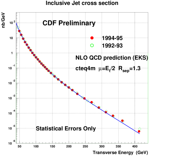
Figure 1:    Data points obtained by CDF [51] compared with the NLO prediction of the theory [52] for the $p_{T}$ distribution of inclusive jet production at factorization and renormalization scale $\mu=p_{t}/2$ with cteq4m parton number densities and the jet separation parameter $R_{\rm sep}=1.3$.

We have a large number of quantitative well tested prediction for deep inelastic scattering, $W/Z$ production, jet-production and heavy quark production. The method of calculation follows of the procedure described above. Both the theoretical and experimental error could be significantly reduced during the last decade and bt now they are about $15\%-30\%$. As illustration of this in Fig. 1 the inclusive transverse energy $E_{T}$ distribution for jet production at Tevatron is shown. The data points obtained by CDF [51] are compared by the absolute NLO QCD prediction [52]. These data are interesting since i) they test the absolute prediction of QCD up to NLO accuracy ii) they give information on the parton number densities at large $Q^{2}$ and iii) they can be used to constrain possible new physics.

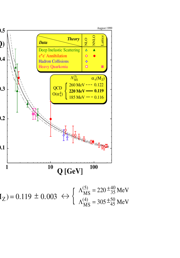
Figure 2: World summary of ${\alpha_{S}}(Q)$ at the energy scales of the experiments  [54].

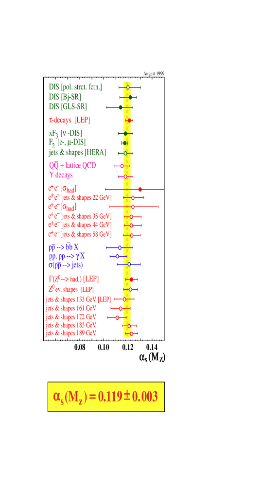
Figure 3: World summary of ${\alpha_{S}}(Q)$ evolved to a common energy scale $Q=M_{\mathrm{Z}}$ [54].

2.1.3 Measurements of ${\alpha_{S}}$

QCD has been discovered by its qualitative properties. Over the last 20 years, however, significant progress has been achieved in the field theoretical techniques for deriving its consequences and by now we can test QCD ${\it quantitatively}$. The free parameters of QCD are the quark masses and the strong coupling constant. Once we fitted these values to some measurable infrared safe quantities, hard scattering processes can be predicted from first principles for $e^{+}e^{-}$ annihilation. For processes with hadrons in the initial state the parton number densities should also be fitted. We do not want to go into this detail (see ref. [53]). The status of QCD tests is well characterized with the agreement between the various values of ${\alpha_{S}}$ extracted from different measurements. We illustrate the present situation with two figures [54]. Fig. 3 gives a test for the running of ${\alpha_{S}}(Q)$ with plotting the value of ${\alpha_{S}}(Q)$ as obtained by various experiments. The data confirms the energy dependence of ${\alpha_{S}}(Q)$ as predicted by QCD. In Fig. 3 we show the summary of the results of the same experiments but evolving the values of ${\alpha_{S}}(Q)$ to a common energy scale, $Q=M_{\mathrm{Z}}$ using the QCD $\beta$ function in ${\cal O}({\alpha_{S}}^{4})$ with 3-loop matching at the heavy quark pole masses $M_{b}=4.7\,{\rm GeV}$ and $M_{c}=1.5\,{\rm GeV}$. The corresponding world average is also given as well as the values of $\Lambda_{\overline{\rm MS}}$ for $n_{f}=4,5$.

2.2 Testing the electroweak theory

In the Standard Model at tree level the gauge bosons $\gamma,W,Z$ and their interactions are described in terms of three parameters: the two gauge coupling constants $g,g^{\prime}$ and the vacuum expectation value of the Higgs field $v$. We need to know their values as precisely as possible. They have to be fitted to the three best measured physical quantities of smallest experimental error: $G_{\mu},M_{\mathrm{Z}}$ and $\alpha$. In leading order we have the simple relations

$$G_{\mu}=\frac{1}{\sqrt{2}v^{2}}\,,\quad M_{\mathrm{Z}}=\frac{1}{2\cos\theta_{W}}gv\,,\quad\alpha=\frac{g^{2}}{4\pi}\sin^{2}\theta_{W}\,,\quad\tan\theta_{W}=\frac{g^{\prime 2}}{g^{2}}\,.$$ (68)

The muon coupling $G_{\mu}$ is extracted from the precise measurement of the muon lifetime using the theoretical expression given by equation (1.2.1)

$$G_{F}=(1.16637\pm 0.00001)\times 10^{-5}\,{\rm GeV}^{-2}\,.$$ (69)

The value of $M_{\mathrm{Z}}$ is extracted from the line shape measurement at the $Z$-pole. There are subtleties in the theoretical definition of the mass and the width at higher order associated with the truncation of the perturbative series and gauge invariance. The latest best value is [55]

$$M_{\mathrm{Z}}=(91.1871\pm 0.0021)\,{\rm GeV}\,.$$ (70)

The best value of $\alpha$ is extracted from the precise measurement of the electron anomalous magnetic moment $(g_{\rm e}-2)$ [28]

$${1}/{\alpha}=137.03599959\pm 0.00000038\,.$$ (71)

Additional physical quantities like the mass of the W-boson $M_{\mathrm{W}}$, the lepton asymmetries at the Z-pole, the leptonic width of the Z-boson $\Gamma_{\rm l}$ etc.  are derived quantities. At the level of the per mil accuracy the predictions obtained in Born approximations for derived quantities, however, disagree with the measured values significantly.

2.2.1 Quantum corrections

At LEP, SLC and Tevatron an enormous amount of data has been collected on the Z and W bosons and their interactions [56, 57]. This allows for an unprecedented precision test of the Standard Model at the level of the per mil accuracy. At this precision one and two-loop quantum fluctuations give measurable contributions and data data show sensitivity also to the Higgs mass and the top mass.

Since the Standard Model is a renormalizable quantum field theory the theoretical predictions of the theory can be improved systematically by calculating higher order corrections. In particular, the recent precision of the data requires the study of the complete next-to-leading order corrections, resummation of large logarithmic contributions and a number of two loop corrections. At higher order the derived quantities show sensitivity also to the values of the mass parameters $m_{t}$, $M_{\mathrm{H}}$, $m_{b}$ and the QCD coupling constant $\alpha_{s}$. From direct measurements one obtains $\alpha_{s}=0.119\pm 0.002$ (see Fig. 3), $m_{t}=173.8\pm 5.0\,{\rm GeV}$ and $\bar{m}_{b}(\bar{m}_{b})=4.25\pm 0.08\,{\rm GeV}$,   $M_{\mathrm{H}}\geq 102{\rm GeV}$ where $\bar{m}_{b}(\bar{m}_{b})$ denotes the $\overline{\rm MS}$ mass [58]. The error bars give parametric uncertainties in the predictions and limit our ability to extract a precise value of the Higgs mass. The calculation of the higher orders requires a choice of the renormalization scheme.

In the perturbation theory the higher order effects can be given in bare and renormalized parameters. Let us consider the basic observables as the basic bare parameters $a_{0}^{i}\equiv(G_{0},\alpha_{0},M_{Z0})$. Calculating the radiative corrections in the regularized theory the radiatively corrected renormalized values of the basic parameters can be written as

$$a^{i}(a^{i}_{0})=a_{0}^{i}+\delta a^{i}(a_{0}^{i})\,.$$ (72)

This relations can be inverted

$$a_{0}^{i}\equiv a_{0}^{i}(a^{i})\,.$$ (73)

Similarly for derived observables we can write

$$O(a_{0}^{i})\equiv O_{0}(a_{0}^{i})+\delta O(a_{0}^{i})\,.$$ (74)

At one loop we can express the radiatively corrected derived quantities as functions of the radiatively corrected basic quantities

$$O(a_{0}^{i}(a_{i})) \approx O_{0}(a_{0}^{i})+\delta O(a_{0}^{i})$$ (75)

$$\approx O_{0}(a^{i})+\delta^{(1)}O(a^{i})-\sum_{i}\frac{\partial O_{0}}{\partial a^{i}}\delta^{(1)}a^{i}$$

$$= O_{0}(a_{i})+\Delta^{(1)}(a^{i})\,.$$

The coefficients of this expansion are finite since we expand renormalized finite quantities in terms of the renormalized finite basic observables. Equation (75), however, tells us that the finite one-loop corrections have a direct part $\delta^{(1)}O$ and an indirect one $-\sum_{i}\frac{\partial O_{0}}{\partial a^{i}}\delta^{(1)}a^{i}$ coming from corrections to the basic parameters. The two contributions can be separately divergent, only the sum is finite.

In the on shell scheme [59] the mixing angle $s^{2}=\sin^{2}\theta$ is defined by the tree level relation $s^{2}=1-M_{\mathrm{W}}^{2}/M_{\mathrm{Z}}^{2}$ in all order, therefore, it is a physical quantity. It is customary to define auxiliary dimensionless parameters $r_{W}$ by the relation

$$s^{2}c^{2}\equiv\frac{\pi\alpha}{\sqrt{2}G_{\mu}M_{\mathrm{Z}}^{2}(1-r_{W})}$$ (76)

where $c^{2}=1-s^{2}$. Obviously $r_{W}$ is also a finite derived quantity and it gives the radiative corrections to the $M_{\mathrm{W}}$.

In the $\overline{\rm MS}$-scheme the measured values of $\alpha$, $G_{\mu}$, $M_{\mathrm{Z}}$, $m_{f}$, ${\alpha_{S}}$ are used to fix the input parameters of the theory with $M_{\mathrm{H}}$ as free parameter. The $\overline{\rm MS}$ gauge couplings evaluated at the scale of $M_{\mathrm{Z}}$ are denoted as $\hat{e}$ and $\hat{s}^{2}=\sin^{2}\hat{\theta}_{W}(M_{\mathrm{Z}})$. The renormalized parameters $\hat{s}^{2}$, $\hat{e}^{2}$ can be completely calculated in terms of $G_{\mu}$, $\alpha$ and $M_{\mathrm{Z}}$. Another useful auxiliary quantity is the effective mixing angle

$$\sin^{2}\theta^{eff}_{W}=\frac{1}{4}\left(1-\frac{\bar{v}_{l}}{\bar{a}_{l}}\right)=s^{2}(1+\Delta k^{{}^{\prime}})\,.$$ (77)

This is uniquely related to the ratio of the effective neutral current vector and axialvector couplings $\bar{v}_{l}$ and $\bar{a}_{l}$ of leptons (see equation (33)) and it gives the leptonic forward-backward asymmetries $A_{FB}^{l}$ at the Z-pole in all order of the perturbation theory as well as the tau polarization $A_{\tau}^{\rm pol}$ and left-right polarization asymmetries $A_{\rm pol}$

$$A_{\rm FB}^{l}=\frac{3}{4}A_{e}A_{f}\,,\quad A^{\rm pol}=A_{\tau}\,,\quad A_{\rm LR}=A_{e}\,$$ (78)

where

$$A_{f}=\frac{2\bar{v}_{v}\bar{a}_{f}}{\bar{v}_{f}^{2}+\bar{a}_{f}^{2}}\,.$$ (79)

Measurements of the asymmetries hence are measurements of the effective mixing angle and therefore it is a physical quantity as well the dimensionless parameter $\Delta k^{{}^{\prime}}$ defined by equation (77). The leptonic width depends on the vector and axial vector coupling and on the corrections to the $Z$-propagator. This requires the introduction of the so called $\rho$-parameter

$$\Gamma_{l}=\frac{G_{\mu}M_{\mathrm{Z}}^{3}}{6\pi\sqrt{2}}\left(\bar{g}_{Vl}^{2}+\bar{g}_{Al}^{2}\right)\rho\,.$$ (80)

The corrections $\Delta r_{W}$, $\Delta k^{\prime}$, $\Delta\rho$ are known in various schemes and play an important role in the analysis of electroweak physics, because they give the precise predictions of the theory for simple observables as $M_{\mathrm{W}}$, the leptonic asymmetries etc.  in terms of $\alpha,G_{\mu}$ and $M_{\mathrm{Z}}$. It is very useful to have the results in different schemes since it allows for cross-checking the correctness of the result and to estimate the remaining theoretical errors given by the missing higher order contributions.

In the precision tests assuming that the analysis is not restricted to the Standard Model the radiative corrections it is convenient to use the $\epsilon$ parameters [60] defined as

$$\epsilon_{1}=\Delta\rho\,,\quad\epsilon_{2}=c^{2}\Delta\rho+\frac{s^{2}\Delta r_{W}}{(c^{2}-s^{2})}\,,\quad\epsilon_{3}=c^{2}\Delta\rho+(s^{2}-c^{2})\Delta k^{{}^{\prime}}\,.$$ (81)

The electroweak radiative corrections are dominated by two leading contributions: the running of the electromagnetic coupling and large $m_{t}$ effects to $\Delta\rho$ $(\Delta\rho_{t}\approx 3G_{\mu}m_{t}^{2}/(8\pi^{2}\sqrt{2}))$. These corrections can be absorbed into the parameters of the Born cross section when we get improved Born approximation.

2.2.2 Running electromagnetic coupling

The running of $\alpha$ is completely given by the photon self energy contributions

$$\alpha(M_{\mathrm{Z}})=\frac{\alpha}{1-\Delta\alpha}$$ (82)

where

$$\Delta\alpha=-{\rm Re}\left({\hat{\Pi}}^{\gamma}(M_{\mathrm{Z}}^{2})\right)=-{\rm Re}\left({\Pi}^{\gamma}(M_{\mathrm{Z}}^{2})\right)+{\rm Re}\left({\Pi}^{\gamma}(0)\right)\,.$$ (83)

The self energy contribution is large ($\approx 6\%$). It can be split into leptonic and hadronic contributions

$$\Delta\alpha=\Delta\alpha_{\rm lept}+\Delta\alpha_{\rm had}$$ (84)

The leptonic part is known up to three loop [61]

$$\Delta\alpha_{\rm lept}=314.97687(16)\times 10^{-4}$$ (85)

and the remaining theoretical error is completely negligible. The hadronic contribution is more problematic as it can not be calculated theoretically with the required precision since the light quark loop contributions have non-perturbative QCD effects. One can extract it, however, from the data using the relation

$$\Delta\alpha_{\rm had} = \frac{\alpha}{3\pi}M_{\mathrm{Z}}^{2}{\rm Re}\int_{4m^{2}_{\pi}}^{\infty}ds\frac{R_{e^{+}e^{-}}(s^{\prime)}}{s^{\prime}(s^{\prime}-M_{\mathrm{Z}}^{2}-i\epsilon)}$$

$$R_{e^{+}e^{-}}(s) = \frac{\sigma(e^{+}e^{-}\rightarrow\ \gamma^{*}\rightarrow\ {\rm hadrons})}{\sigma(e^{+}e^{-}\rightarrow\ \mu^{+}\mu^{-})}\,.$$ (86)

Conservatively, one calculates the high energy $\sqrt{s}\geq 40\,{\rm GeV}$ contribution using perturbative QCD. The low energy contribution $\sqrt{s}\leq 40\,{\rm GeV}$ is estimated using data [62]. Unfortunately, the precision of the low energy data is not good enough and the error from this source dominates the error of the theoretical predictions

$$\Delta\alpha_{\rm had}=0.02804\pm 0.00064\,,\\ \alpha^{-1}(M_{\mathrm{Z}})=128.89\pm 0.09\,.$$ (87)

One can, however, achieve a factor of three reduction of the estimated error assuming that the theory can be used down to $\sqrt{s}=m_{\tau}$ when quark mass effects can be included up to three loops. Such an analysis is quite well motivated by the successful results on the tau lifetime. In the hadronic vacuum polarization the non-perturbative power corrections appear to be suppressed and the unknown higher order perturbative contributions are relatively small. In this theory driven approach the error is reduced to an acceptable $0.25\%$ value

$$\alpha^{-1}(M_{\mathrm{Z}})=128.905\pm 0.036\,.$$ (88)

It is unlikely that the low energy hadronic total cross section will be measured in the foreseeable future with a precision leading to essential improvement.

2.2.3 Calculation of $\Delta\rho_{t}$

We have noted in section 1.26 that in the limit of custodial symmetry in leading order $\rho=1$ and the dominant radiative correction comes from the virtual effects of the top quark since the top-bottom mass splitting gives the largest violation of custodial symmetry. The importance of this correction was first pointed out by Veltman [63]. It is an elegant technical trick to calculate this correction using the effective field theory obtained in the $m_{t}\rightarrow\infty$ limit [64]. In this limit we need to keep only the third generation and the gauge bosons can be treated as external classical currents without kinetic terms. The Standard Model Lagrangian can be reduced to the terms

$${\cal L}_{\rm eff}=i\overline{\psi}^{Q}_{L}\gamma_{\mu}D^{\mu}\psi^{Q}_{L}+i\overline{\psi}^{t}_{R}\gamma_{\mu}D^{\mu}\psi^{t}_{R}+i\overline{\psi}^{b}_{R}\gamma_{\mu}D^{\mu}\psi^{b}_{R}+\lambda_{t}\overline{\psi}^{Q}_{L}\Phi\psi^{t}_{r}-V(\Phi)$$ (89)

with the Higgs doublet

$$\Phi=\left(\begin{array}[]{c}\phi^{+}\\ \frac{1}{\sqrt{2}}(v+h+i\chi)\end{array}\right)$$ (92)

where $\chi$ and $\phi^{+}$ are the Goldstone bosons. The renormalized Lagrangian then has the form

$${\cal L}_{\rm eff}=Z_{2}^{\phi}\left|\partial_{\mu}\phi^{+}-i\frac{gv}{2}W^{+}_{\mu}\right|^{2}+\frac{Z_{2}}{2}^{\chi}\left|\partial_{\mu}\chi-i\frac{gv}{2c}Z_{\mu}\right|^{2}+\frac{Z_{h}}{2}\left(\partial_{\mu}h\right)^{2}+...$$ (93)

where we dropped the top and bottom kinetic energy terms, the top mass terms and the gauge boson fermion couplings. In this limit the gauge boson couplings do not get corrections but the $Z$ and $W$ mass terms are modified by the self energy corrections of the Goldstone bosons

$$M_{\mathrm{W}}^{2}=Z_{2}^{\phi}\frac{g^{2}v^{2}}{4}\,,\quad M_{\mathrm{Z}}^{2}=Z_{2}^{\chi}\frac{g^{2}v^{2}}{4c^{2}}$$ (94)

and therefore the correction to the $\rho$ parameter is

$$\Delta\rho=\frac{Z_{2}^{\phi}}{Z_{2}^{\chi}}-1$$ (95)

that is we can get the correction to the $\rho$ parameter simply by calculating the the contributions of top and top-bottom fermion loops to difference of the self energies of the neutral and charged Goldstone bosons. Carrying out this simple calculation we can easily check that the answer is

$$\Delta\rho_{t}\approx 3\frac{G_{F}m_{t}^{2}}{8\pi\sqrt{2}}.$$ (96)

The method can be extended to two loop order and the corresponding two loop calculation has been carried out in  [64] confirming previous result [65].

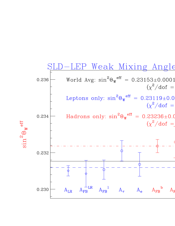
Figure 4:          Summary of all the determinations of $\sin^{2}\theta_{W}^{\rm eff}$ [56].

2.2.4 Higher order corrections to $M_{\mathrm{W}}$ and the mixing angle

As we noted above, the simplest physical observables for precise tests of the Standard Model are $M_{\mathrm{W}}$ and the $\sin^{2}\theta^{eff}_{W}$. It is convenient to consider the radiative corrections in the $\overline{\rm MS}$ scheme where with good accuracy $\sin^{2}\theta^{eff}_{W}\approx\hat{s}^{2}$. It is given in terms of the input parameters via the relation

$$\hat{s}^{2}\hat{c}^{2}=\frac{\pi\alpha(M_{\mathrm{Z}})}{\sqrt{2}G_{\mu}M_{\mathrm{Z}}^{2}(1-\hat{r}_{W})}$$ (97)

where $\hat{r}_{W}=0$ in leading order. Using the measured value of $\sin^{2}\theta^{eff}_{W},M_{\mathrm{Z}}$ and $G_{\mu}$ we obtain a value $\hat{r}_{W}=0.0058\pm 0.000480$ different from zero at the $12\sigma$ level. If one carries out a similar analysis for $M_{\mathrm{W}}$ the evidence for the presence of subleading corrections is even better. The radiative correction $\hat{r}_{W}$ does not contain the large effect from the running $\alpha$ but it receives large custodial symmetry violating corrections because of the large top-bottom mass splitting

$$\Delta\hat{r}_{W}|_{\rm top}=-c^{2}/s^{2}\Delta\rho\approx 0.0096\pm 0.00095\,.$$ (98)

Subtracting this value we get about $6\sigma$ difference coming from the loops involving the bosonic sector (W,Z,H) and subleading fermionic contributions. At this level of accuracy many other corrections start to become important and the size of errors coming from the errors in the input parameters leads to effects of the same order. In particular, we get some sensitivity to the value of the Higgs mass. Beyond the complete one loop corrections it was possible to evaluate all important two loop corrections: ${\cal O}(\alpha^{2}\ln(M_{\mathrm{Z}}/m_{f})$ corrections with light fermions, mixed electroweak QCD corrections of ${\cal O}(\alpha\alpha_{s})$, two loop electroweak corrections enhanced by top mass effects of ${\cal O}(\alpha^{2}(m_{t}^{2}/M_{\mathrm{W}}^{2})^{2})$ together with the subleading parts of ${\cal O}(\alpha\alpha_{s}^{2}m_{t}^{2}/M_{\mathrm{W}}^{2})$ and the very difficult subleading correction of ${\cal O}(\alpha^{2}m_{t}^{2}/M_{\mathrm{W}}^{2})$. It is remarkable that this last contribution proved to be important in several respect [66]. Its inclusion reduced significantly the scheme dependence of the results and lead to a significant reduction of the upper limit on the Higgs mass.

2.2.5 Global fits

This summer the LEP experiments and SLD could finalize their results on the electroweak precision data. The most important development is that the final value of SLD on the leptonic polarization asymmetry which implies $\sin^{2}\theta^{eff}_{W}=0.23119\pm 0.00020$. A nice summary of the results is given in Fig. 4. According to a recent analysis of the EWWW working group [55], the new world average is

$$\sin^{2}\theta^{eff}_{W}=0.23151\pm 0.00017{\rm\ \ \ with\ \ \ }\chi^{2}/{\rm d.o.f=13.3/7}\,.$$ (99)

This gives only rather low confidence level of $6.4\%$. The origin of this unsatisfactory result is the $2.9\sigma$ discrepancy between the values $\sin^{2}\theta^{eff}_{W}$ deriving from the SLAC leptonic polarization asymmetry data and from the forward backward asymmetry in the b-b channel at LEP and SLC. The results obtained from a global fit to all data give somewhat better result but there we are hampered with the problem that the polarization asymmetry parameters disagree with each other with $2.7\sigma$, therefore the $\chi^{2}$ is relatively large.

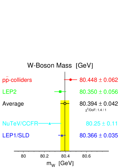
Figure 5:           Summary of the measured values of $M_{\mathrm{W}}$ [56].

2.2.6 Upper limit on $M_{\mathrm{H}}$

The final results of the electroweak radiation corrections for $M_{\mathrm{W}}$ and $\sin^{2}\theta^{eff}_{W}$ can be parameterized in terms of the input parameters including their errors in simple approximate analytic form [66]. For example in the $\overline{MS}$-scheme one obtains for the W-mass

$$M_{\mathrm{W}} = 80.3827-0.0579\ln(\frac{M_{\mathrm{H}}}{100})-0.008\ln^{2}(\frac{M_{\mathrm{H}}}{100})$$ (100)

$$-0.517\left(\frac{\Delta\alpha_{h}^{(5)}}{0.0280}-1\right)+0.543\left[\left(\frac{m_{t}^{2}}{175}-1\right)\right]$$

$$-0.085\left(\frac{\alpha_{s}(M_{\mathrm{Z}})}{0.118}-1\right)$$

where $m_{t}$, $M_{\mathrm{H}}$ and $M_{\mathrm{W}}$ are in $\,{\rm GeV}$ units. This formula accurately reproduces the result obtained with numerical evaluation of all corrections in the range $75\,{\rm GeV}\leq M_{\mathrm{H}}\leq 350\,{\rm GeV}$ with maximum deviation of less than $1\,{\rm MeV}$. In Fig. 5 the measured values of $M_{\mathrm{W}}$ are summarized [56]. Using the world average $M_{\mathrm{W}}=80.394\pm 0.042\,{\rm GeV}$ with input parameters $\alpha_{s}=0.119\pm 0.003$, $m_{t}=174.3\pm 5.1\,{\rm GeV}$, $\delta\alpha^{(5)}=0.02804\pm 0.00065$ one obtains at $95\%$ confidence level an allowed range for the Higgs mass of $73\,{\rm GeV}\leq M_{\mathrm{H}}\leq 294\,{\rm GeV}$. Similar result exists also for $\sin^{2}\theta^{eff}_{W}$ extracted from the asymmetry measurements at the Z-pole with somewhat better (95% confidence) limits of $95\,{\rm GeV}\leq M_{\mathrm{H}}\leq 260\,{\rm GeV}$. Without global fits we got a semi-analytic insight on the sensitivity of the precision tests to the Higgs mass. We also see that the precise measurements of $M_{\mathrm{W}}$ have already provided us with competitive values in comparison with those obtained from the measurement of $\sin^{2}\theta^{eff}_{W}$.

It is interesting that the values of the Higgs mass obtained in a recent global fit [67] are in good agreement with the simple analysis based on the value of $M_{\mathrm{W}}$ or $\sin^{2}\theta^{eff}_{W}$ as described above. One obtains an expected value for the Higgs boson of $160-170\,{\rm GeV}$ with error of $\pm 50-60\,{\rm GeV}$. The 95% confidence level upper limit is about $260-290\,{\rm GeV}$. In Fig. 6 $\Delta\chi^{2}$ is plotted as the function of $M_{\mathrm{H}}$.

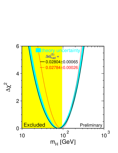
Figure 6: Significance of the global fit as a function of the Higgs mass [55].

2.2.7 Can the Higgs boson be heavy?

The precision data can not yet rule out dynamical symmetry breaking with some heavy Higgs like scalar and vector resonances. The minimal model to describe this alternative is obtained by assuming that the new particles are heavy (more than 0.5  TeV) and the linear $\sigma$-model Higgs sector of the Standard Model is replaced by the non-renormalizable non-linear $\sigma$-model. It can be derived also as an effective chiral vector-boson Lagrangian with non-linear realization of the gauge symmetry [68, 69]. How can we reconcile this more phenomenological approach with the precision data? Removing the Higgs boson from the Standard Model while keeping the gauge invariance is a relatively mild change. Although the model becomes non-renormalizable, at the one-loop level the radiative effects grow only logarithmically with the cut-off at which new interactions should appear. In equation (100) the Higgs mass is replaced by this cut-off. The logarithmic terms are universal, therefore their coefficients must remain the same. The constant terms, however, can be different from those of the Standard Model. The one loop corrections of the effective theory require the introduction of new free parameters which influence the value of the constant terms. The data, unfortunately, do not have sufficient precision to significantly constrain the constant terms appearing in $M_{W}$, $\sin^{2}\theta^{eff}_{W}$ and $\Gamma_{l}$ (or alternatively in the parameters $\epsilon_{1},\epsilon_{2},\epsilon_{3}$ [60] or $S,T,U$ [70] ). In a recent analysis  [71] it has been found that due to the screening of the symmetry breaking sector [72], alternative theories with dynamical symmetry breaking and heavy scalar and vector bosons still can be in agreement with the precision data up to a cut-off scale of $3{\rm TeV}$.

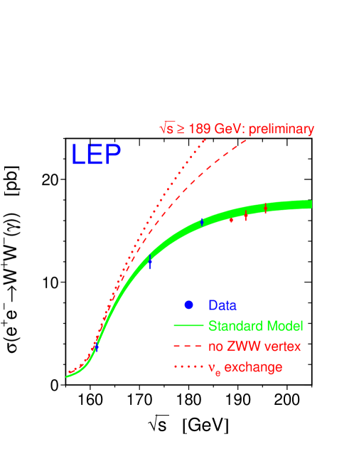
Figure 7: The W-pair production cross-section as function of the center-of-mass energy [55]. The data points are the LEP averages. Also shown is the Standard Model prediction [73] (shaded area) with a possible uncertainties of $\pm 2\%$ of the calculations. For comparison the cross sections are also shown if the ZWW coupling did not exist (dashed line), or if only the t-channel $\nu_{e}$ exchange diagram existed (dotted line).

2.2.8 W-pair production

At LEP the precise measurement of the production of $W^{+}W^{-}$ is also an important physics goal. The production of gauge boson pairs provide us with the best test of the non-Abelian gauge symmetry of the Standard Model. Deviation from the Standard Model predictions may come either from the presence of anomalous couplings or the production of new heavy particles and their decays into vector-boson pairs. If the particle spectrum of the Standard Model has to be enlarged with new particles (as in the Minimal Supersymmetric Standard Model) with mass values of $\geq 0.5-1{\rm TeV}$, small anomalous couplings are generated at low energy. In Fig. 7 we show the recent measurement of the W-pair cross-section.

3 HIGGS SECTOR, HIGGS SEARCH

3.1 Difficulties with the Higgs sector

The Standard Model is defined only in perturbation theory, but the perturbative treatment of the Higgs sector can not be valid up to arbitrary high energies. Its range of validity depends strongly on the value of the Higgs mass.

Figure 8: Bounds on $M_{H}$ as as a function of the cut-off scale $\Lambda$. The upper solid area indicates the the triviality upper bound. The width of the area indicates the sum of the theoretical uncertainties in the $M_{\mathrm{H}}$. The lower solid area represents the lower bounds derived from stability requirements using $m_{t}=175\,{\rm GeV}$ and ${\alpha_{S}}=0.118$ [77, 78].

3.1.1 Theoretical upper limits on $M_{\mathrm{H}}$

For high Higgs mass values we get conflict with perturbative unitarity [74] since according to equation (46) if $M_{\mathrm{H}}>>M_{\mathrm{W}}$ the scalar self interaction becomes strong. Unitarity requires that in a given angular momentum channel the scattering matrix element fulfills the relations

$$\left|M_{J}\right|^{2}\leq\left|{\rm Im}(M_{J})\right|\,,\quad\left|{\rm Re}(M_{J})\right|\,<\frac{1}{2}$$ (101)

Applying these constraints for the Born amplitude of $W_{L}W_{L}$ scattering we get

$$M_{\mathrm{H}}^{2}\leq\frac{2\pi\sqrt{2}}{G_{F}}\approx(850\,{\rm GeV})^{2}$$ (102)

A more precise coupling channel analysis leads to somewhat better limit

$$M_{\mathrm{H}}^{2}\leq\frac{2\pi\sqrt{2}}{G_{F}}\approx(700\,{\rm GeV})^{2}\,.$$ (103)

If the Higgs self coupling is large, the gauge interactions are negligible. The scalar interaction, however, is not asymptotically free, therefore in the perturbation theory the running coupling constant has a Landau pole. Actually it has been proven that the scalar theory is trivial [75]. If we require to have finite scalar coupling at very short distances we get vanishing coupling at large distances: the theory becomes free. The scalar sector mathematically can not be rigorous and it should be considered as an effective low energy theory. The scalar self coupling $\lambda$, therefore, has to be smaller than its value at the Landau pole. This condition also gives an upper limit on $M_{\mathrm{H}}$. The one loop running coupling is

$$\lambda(\mu)=\frac{\lambda(M_{\mathrm{H}})}{1-12\frac{\lambda(M_{\mathrm{H}})}{16\pi^{2}}\ln\frac{\mu^{2}}{M_{\mathrm{H}}^{2}}}$$ (104)

where $\lambda(M_{\mathrm{H}})=g^{2}M_{\mathrm{H}}^{2}/(8M_{\mathrm{W}}^{2})$. The position of the Landau pole is at the scale

$$\mu_{c}=M_{\mathrm{H}}e^{\frac{2\pi^{2}}{3\lambda(M_{\mathrm{H}})}}=M_{\mathrm{H}}e^{\frac{16\pi^{2}M_{\mathrm{W}}^{2}}{3g^{2}M_{\mathrm{H}}^{2}}}$$ (105)

the condition $\mu_{c}>2M_{\mathrm{H}}$ leads to the upper limit

$$M_{H}<700{\rm GeV}\,.$$ (106)

If the Landau pole is pushed up to the Planck scale we get the more stringent limit of $M_{\mathrm{H}}<170\,{\rm GeV}$. This is a tentative estimate since perturbation theory is used beyond its range of validity. Note that non-perturbative lattice studies [76] give very similar value $M_{\mathrm{H}}<650\,{\rm GeV}$. One can redo the analysis at two loop order when the two loop beta function has a metastable fixed point. With the assumption that the theory is meaningful up to a scale where the coupling constant is half of the value of the coupling at the metastable fixed point one, gets again similar upper limit [77, 78, 79].

3.1.2 Lower limits on $M_{\mathrm{H}}$

The requirement of stability of the Higgs potential $V(\phi)>0$ leads to a lower limit on the Higgs mass. The $\beta$-function of the scalar self-interaction is

$$\beta_{\lambda} = \frac{1}{8\pi^{2}}\bigl{[}12\lambda^{2}-3g_{t}^{4}+6\lambda g_{t}^{2}-\frac{\lambda}{2}(9g^{{}^{\prime}2}+3g^{2})$$ (107)

$$+\frac{3}{16}(3g^{{}^{\prime}4}+2g^{{}^{\prime}2}g^{2}+g^{4})\bigr{]}$$

where $g_{t}=gm_{t}/(2M_{\mathrm{W}})$ denotes the top quark Yukawa coupling. At large top mass and small $\lambda$ the second term will dominate, as we get negative $\beta$ function and $\lambda$ will decrease with increasing top mass and $V(\Phi)$ can become negative. A coupled channel analysis at two loop order leads to the approximate relation (assuming that the theory is meaningful up to the Planck scale) $M_{\mathrm{H}}>1.95m_{t}-190\,{\rm GeV}$ and for $m_{t}=175\,{\rm GeV}$ one gets the lower limit $M_{\mathrm{H}}>150\,{\rm GeV}$. So the Higgs boson should not be found at LEP2 in this case. In Fig. 8 theoretical upper and lower bounds on $M_{H}$ are shown as a function of the scale charaterizing the range of validity (cut-off scale) of the Standard Model. We can see that if $M_{\mathrm{H}}\approx 165-195\,{\rm GeV}$ the cut-off scale can extend up to the Planck scale. I should recall, however, that this is rather unlikely since the mass term of the scalar boson is a relevant operator, therefore, it is linearly sensitive of the scale of new physics. The question “why is the Higgs mass so light with respect to the Planck scale” is referred to in literature as the gauge hierarchy problem.

3.2 Search at LHC

One of the most important physics goal at the LHC is to obtain decisive experimental test on the Higgs sector of the Standard Model [80, 81]. The experimental prospects are summarized with the so called “no loose scenario”

• either the Higgs boson will be discovered at LEP2 or LEP2 will establish a lower limit of $m_{H}>107\,{\rm GeV}$;

• assuming the validity of the minimal Higgs sector the precision data obtained at LEP1 and SLC constrain the value of $M_{\mathrm{H}}$ to be less than $\approx 295\,{\rm GeV}$.

• LHC will be able to discover the Standard Model Higgs boson in the interval $800\,{\rm GeV}>m_{H}>107\,{\rm GeV}$ or will find clear evidence for deviations from Standard Model predictions.

To be able to make maximal use of the results of the LHC experiments one should calculate the Standard Model predictions for LHC processes as precisely as possible. It is unsatisfactory that the present experimental simulation studies are based on leading order cross sections. Nevertheless at the parton level most of the NLO corrections are available and are public in form of program packages [82]. HDECAY generates all branching fractions of the Standard Model Higgs boson and the Higgs bosons of the Minimal Supersymmetric Standard Model (MSSM), while HGLUE provides the production cross sections of the SM and MSSM Higgs bosons via gluon fusion including the NLO QCD corrections.

3.2.1 Higgs branching ratios

The branching ratios of the Higgs boson have been studied in many papers. A useful compilation of the early works on this subject can be found in Ref. [80], where the most relevant formulae for on-shell decays are summarized. Higher-order corrections to most of the decay processes have been computed (for up-to-date reviews see Refs. [83] and references therein).

The bulk of the QCD corrections to $H\rightarrow q\bar{q}$ can be absorbed into a ‘running’ quark mass $m_{q}(\mu)$, evaluated at the energy scale $\mu=M_{H}$. The importance of this effect for the case $q=b$, with respect to intermediate-mass Higgs searches at the LHC, has been discussed already in Ref. [84]. For sake of illustration, results on the Higgs branching ratios are summarized in Fig. 9. Branching ratios are depicted as function of $M_{\mathrm{H}}(M_{\mathrm{H}}\leq 200~{}\,{\rm GeV})$ for channels: (a) $b\bar{b}$, $c\bar{c}$, $\tau^{+}\tau^{-}$, $\mu^{+}\mu^{-}$ and $gg$; and for channels (b) $WW$, $ZZ$, $\gamma\gamma$ and $Z\gamma$. The patterns of the various curves are not significantly different from those presented in Ref. [84]. The inclusion of the QCD corrections in the quark-loop induced decays give a change of at most a few per cent for the decays $H\rightarrow\gamma\gamma$ and $H\rightarrow Z\gamma$, while for $H\rightarrow gg$ differences are of order 50–60%. However, this latter result has little phenomenological relevance, since this decay width makes a negligible contribution to the total width, and in practice it is an unobservable channel.

Figure 9: Branching ratios of the Higgs boson in the mass range 50 GeV $<M_{H}<$ 200 GeV, for the decay modes: a) $b\bar{b}$, $c\bar{c}$, $\tau^{+}\tau^{-}$, $\mu^{+}\mu^{-}$ and $gg$; b) $WW$, $ZZ$, $\gamma\gamma$ and $Z\gamma$ [85] .

Figure 10: Feynman diagram for various production mechanisms.

Figure 11: Total cross sections for $H$ production at the LHC as a function of the Higgs mass $M_{H}$, given by the four production mechanisms illustrated in Fig. 10, at $\sqrt{s}_{pp}=14$ TeV .

Figure 12: Higgs production cross sections times the branching ratios for the decay modes $H\rightarrow W^{(*)}W^{(*)}\rightarrow\ell^{+}\nu_{\ell}\ell^{\prime-}\bar{\nu}_{\ell^{\prime}}$ ($\ell,\ell^{\prime}=e,\mu$) and $H\rightarrow Z^{(*)}Z^{(*)}\rightarrow\ell^{+}\ell^{-}\ell^{\prime+}\ell^{\prime-}\,$ as a function of the Higgs mass in the range $0\leq M_{H}\leq 300$ GeV, at $\sqrt{s}_{pp}=10$ TeV and $\sqrt{s}_{pp}=14$ TeV with $m_{t}=175$ GeV.

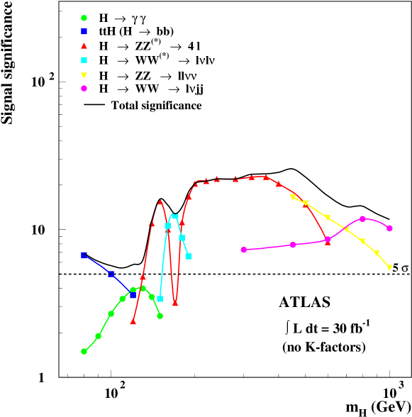
Figure 13: Signal significance as function of the Higgs mass $M_{H}$ for the ATLAS experiment. The statistical significances are plotted for individual channels as well as combination of all channels assuming integrated luminosity of 30 $\rm fb^{-1}$. Depending on the numbers of signal (S) and background (B)events, the statistical significance has been computed as $S/\sqrt{B}$ [99].

3.2.2 Higgs production cross sections and event rates

There are only four Higgs production mechanisms which lead to detectable cross sections at the LHC: a) gluon-gluon fusion [86], b) $WW$, $ZZ$ fusion [87], c) associated production with $W$, $Z$ bosons [88], d) associated production with $t\bar{t}$ pairs [89]. Each mechanism involves heavy particles. Representative Feynman diagrams are shown in Fig. 10. Again for illustrative purpose in Fig. 11 total cross-section values are depicted for LHC energies$\sqrt{s}=14~{}\,{\rm TeV}$ . There are various uncertainties in the rates of the above processes, although none is particularly large. They are given by the lack of precise knowledge of the gluon distribution at small $x$ and by effects of unknown higher-order perturbative QCD corrections [85].

The next-to-leading order QCD corrections are known for processes (a), (b) and (c) and are included. By far the most important of these are the corrections to the gluon fusion process calculated in Ref. [90]. Within the limit where the Higgs mass is far below the $2m_{t}$ threshold, these corrections are calculable analytically [91, 92]. In fact, it turns out that the analytic result is a good approximation up to the threshold $M_{\mathrm{H}}<2m_{t}$ [93, 94]. In Ref. [94, 85] the impact of the next-to-leading order QCD corrections for the gluon fusion process on LHC cross sections has been investigated, both for the SM and for the MSSM. Overall, the next-to-leading order correction increases the leading order result by a factor of about 2, when the normalization and factorization scales are set equal to $\mu=M_{H}$. This ‘$K$-factor’ can be traced to a large constant piece in the next-to-leading correction [90]

$$K\approx 1+{\alpha_{s}(M_{H})\over\pi}\;\left[{\pi^{2}}+{11\over 2}\right].$$ (108)

Such a large $K$-factor usually implies a non-negligible scale dependence of the theoretical cross section.

To judge the quality of the various signals of Higgs production, we must know event rates both for the signals and the backgrounds. Considering all the possible combinations of production mechanisms and decay channels [95, 96], the best chance of discovering a Higgs at the LHC are given by the signatures: (i) $gg\rightarrow H\rightarrow\gamma\gamma$, (ii) $q\bar{q}^{\prime}\rightarrow WH\rightarrow\ell\nu_{\ell}\gamma\gamma$ and (iii) $gg\rightarrow H\rightarrow Z^{(*)}Z^{(*)}\rightarrow\ell^{+}\ell^{-}\ell^{\prime+}\ell^{\prime-}$, where $\ell,\ell^{\prime}=e$ or $\mu$. By exploiting techniques of flavor identification of $b$-jets, thereby reducing the huge QCD background from light-quark and gluon jets, the modes (iv) $q\bar{q}^{\prime}\rightarrow WH\rightarrow\ell\nu_{\ell}b\bar{b}$ and (v) $gg,q\bar{q}\rightarrow t\bar{t}H\rightarrow b\bar{b}b\bar{b}WW\rightarrow b\bar{b}b\bar{b}\ell\nu_{\ell}X$, can also be used to search for the Higgs [97]. Another potentially important channel, particularly for the mass range $2M_{W}\buildrel\scriptscriptstyle<\over{\scriptscriptstyle\sim}M_{H}\buildrel\scriptscriptstyle<\over{\scriptscriptstyle\sim}2M_{Z}$, is (vi) $H\rightarrow W^{(*)}W^{(*)}\rightarrow\ell^{+}\nu_{\ell}\ell^{\prime-}\bar{\nu}_{\ell^{\prime}}$ [98]. Here the lack of a measurable narrow resonant peak is compensated by a relatively large branching ratio, since for this mass range $H\rightarrow WW$ is the dominant decay mode. Again for sake of illustration we show in Fig. 12 Higgs production times branching ratios for various decay modes at two different energies.

The potential of the ATLAS experiment for the discovery of the Standard Model Higgs boson in the mass range $80\,{\rm GeV}<M_{\mathrm{H}}<1\,{\rm TeV}$ is summarized in Fig. 13. The significance of the signal depends on the signal (S) and background events and is given by $S/\sqrt{B}$. The results shown in the figure are obtained from calculating the event rates both for the background and the signal in the Born approximation. It is argued that since the QCD corrections are not known for all signal and background processes, it is more consistent to neglect them everywhere. Hopefully this shortcomings will be eliminated soon. One can consider these result conservative since the QCD corrections are large for the signal and there is no reason to assume that they are even larger for the background.

References

- [1]
- [2] G. ’t Hooft, Singapore, World Scientific (1994) 683 p. (Advanced series in mathematical physics, 19).
- [3] R. P. Feynman, Phys. Rev. Lett. 23 (1969) 1415.
- [4] G. ’t Hooft, Nucl. Phys. B33 (1971) 173.
- [5] G. ’t Hooft, Nucl. Phys. B35 (1971) 167.
- [6] H. Fritzsch and M. Gell-Mann, Proc. XVI Intern. Conf. on High Energy Physics, Chicago, (1972), Vol.2. p135
- [7] H. Fritzsch, M. Gell-Mann and H. Leutwyler, Phys. Lett. B47 (1973) 365.
- [8] G. ’t Hooft, Marseilles Conference on Renormalization, June 1972, (unpublished).
- [9] D. J. Gross and F. Wilczek, Phys. Rev. Lett. 30 (1973) 1343.
- [10] D. Politzer, Phys. Rev. Lett. 30 (1973) 1346.
- [11] D. J. Gross and F. Wilczek, Phys. Rev. D8 (1973) 3633.
- [12] K. Wilson, Phys. Rev. D10 (1974) 2445.
- [13] G. ’t Hooft, Nucl. Phys. B190 (1981) 455.
- [14] R. W. Haymaker, Phys. Rep. 315 (1999) 153 .
- [15] G. ’t Hooft, Nucl. Phys. B79 (1974) 276; Nucl. Phys. B105 (1976) 538.
- [16] A. M. Polyakov, JETP Letter 20 (1974) 1 974.
- [17] G. ’t Hooft, Phys. Rev. D14 (1976) 3432.
- [18] QCD descibed in a number of monographs, e.g. G. Sterman, Introduction to Quantum Field Theory, Cambridge (1993); M. E. Peskin and D. V. Schröder, An Introduction to Qunatum Field Theory, Addison-Wesley (1995); Yu. L. Dokshitzer et al. Basics of Perturbative QCD, Editions Frontiers (1989); F. Yndurain, Quantum Chormodynamics, Springer-Verlag (1983); T. Muta, Foundation of Quantum Chromodynamics, World Scientific, Second Edition (1998); Perturbative Quantum Chromodynamics Edited by A. H Mueller, World Scientific (1989) .
- [19] R. D. Peccei and H. R. Quinn, Phys. Rev. Lett. 38 (1977) 1440.
- [20] G. ’t Hooft and M. Veltman, Nucl. Phys. B50 (1972) 318.
- [21] G. ’t Hooft and M. Veltman, Nucl. Phys. B44 (1972) 189.
- [22] I. Montvay and G. Munster, Quantum Fields on a Lattice. Cambridge (1997) .
- [23] G. ’t Hooft, Phys. Rev. Lett. 37 (1976) 8.
- [24] J. Gasser and H. Leutwyler, Nucl. Phys. B250 (1985) 465.
- [25] M. Neubert, Phys. Rep. 245 (1994) 259
- [26] C. S. Wu, E. Ambler, R. W. Hayward, D. D. Hoppes and R. P. Hudson, Phys. Rev. 105 (1957) 1413.
- [27] T. D. Lee and C. N. Yang, Phys. Rev. 104 (1956) 254.
- [28] C. Caso et al., Eur. Phys. J. C3 1 (1998).
- [29] S. M. Berman and A. Srilin, Ann. Phys. (NY) 20 (1962) 20.
- [30] T. Kinoshita, Phys. Rev. Lett. 2 (1959) 477 .
- [31] T. van Ritbergen and R. G. Stuart, Phys. Rev. Lett. 82 (1999) 488 .
- [32] S. L. Glashow, Nucl. Phys. B22 (1961) 22 .
- [33] S. Weinberg, Phys. Rev. Lett. 19 (1967) 1264 ; A. Salam, Proc. 8th Nobel Symposium, (1968), ed. N. Svart;
- [34] M. Veltman, Nucl. Phys. B7 (1968) 637.
- [35] P. W. Higgs, Phys. Rev. Lett. 13 (1964) 508.
- [36] F. Englert and R. Brout, Phys. Rev. Lett. 13 (1964) 321 .
- [37] Y. Fukuda et al. [Super-Kamiokande Collaboration], Phys. Rev. Lett. 81 (1998) 1562.
- [38] S. L. Glashow, J. Iliopoulos and L. Maiani, Phys. Rev. D2 (1970) 1285.
- [39] L. Wolfenstein, Phys. Rev. Lett. 51 (1983) 1945.
-
[40]
A. J. Buras, M. Ciuchini, E. Franco, G. Isidori, G. Martinelli and L. Silvestrini,
hep-ph/0002116. - [41] C. Jarlskog, Phys. Rev. Lett. 55 (1985) 1039.
- [42] T. Kinoshita, J. Math. Phys. 3 (1965) 56 ; T. D. Lee and M. Nauenberg Phys. Rev. 133 (1964) 1549 .
- [43] D. Amati and G. Veneziano, Nucl. Phys. B140 (1978) 54 ; R .K. Ellis, H. Georgi, M. Machacek,H. D. Politzer and G. G. Gross Nucl. Phys. B152 285 79 ; A. V. Efremov and A. V. Radyushkin, Theor. Math. Phys. 44 (1980) 17 ; S. Libby and G. Sterman, Phys. Rev. D18 (1978) 3252 A. Mueller, Phys. Rev. D18 (1978) 3705
- [44] G. Bodwin, Phys. Rev. D31 (1986) 2616 ; ibid D34 (1986) 3932 ; J. C. Collins, D. E. Soper and G. Sterman, Nucl. Phys. B261 (1986) 104 ; ibid B308 (1988) 833
- [45] J. C. Collins and D. E. Soper, Ann. Rev. Nucl. Part. Sci. 37 (1987) 383 ; J. C. Collins, D. E. Soper and G. Sterman, in Perturbative QCD, ed. A.H. Mueller (World Scientific 1989)
- [46] K. G. Chetyrkin, A. L. Kataev and F. V. Tkachov, Phys. Lett. B85 (1979) 277 ; M. Dine and J. Sarpinstein, Phys. Rev. Lett. 43 (1979) 688 ; W. Celemaster and R. Gonsalves, Phys. Rev. Lett. 44 (1980) 560 .
- [47] G. Sterman and S. Weinberg, Phys. Rev. Lett. 39 (1977) 1436 .
- [48] J. C. Collins and D. E. Soper, Ann. Rev. Nucl. Part. Sci. 37 383 87 ; J. C. Collins, D. E. Soper and G. Sterman, in ‘Perturbative QCD’, ed. A.H. Mueller, World Scientific (1989).
- [49] G. Altarelli and G. Parisi, Nucl. Phys. B126 (1977) 298.
- [50] M. L. Mangano, hep-ph/9911256.
- [51] F. Abe et. al., CDF Collab. Phys. Rev. Lett. 77 (1996) 437.
- [52] S. D. Ellis, Z. Kunszt and D. E. Soper, Phys. Rev. Lett. 64 (1990) 2121.
- [53] R. K. Ellis, W. J. Stirling and B. R. Webber, QCD and Collider Physics, Cambridge University Press (1996).
- [54] S. Bethke, hep-ex/0001023.
- [55] LEP and SLD Electroweak Working Group, preprint CERN EP/2000-16.
- [56] M. L. Swartz, hep-ex/9912026 and references therein.
- [57] A. Sirlin, hep-ph/9912227 and references therein.
- [58] M. Beneke and A. Signer, Phys. Lett. B471 (1999) 233.
- [59] D. Bardin and G. Passarino, The Standard Model in the Making, Clarendon Press, Oxford (1999).
- [60] G. Altarelli and R. Barbieri, Phys. Lett. B253 (1991) 161; G. Altarelli, R. Barbieri and F. Caravaglios, Nucl. Phys. B405 3 (1993) .
- [61] M. Steinhauser, Phys. Lett. B429 (1998) 158.
- [62] F. Jegerlehner, hep-ph/9901386.
- [63] M. Veltman, Nucl. Phys. B123 (1977) 89.
-
[64]
R. Barbieri, M. Beccaria, P. Ciafaloni, G. Curci and A. Vicere,
Nucl. Phys. B409 (1993) 105. - [65] J. J. van der Bij and F. Hoogeveen, Nucl. Phys. B283 (1987) 477.
- [66] G. Degrassi and P. Gambino, hep-ph/9905472.
- [67] G. D’Agostini and G. Degrassi, hep-ph/0001269.
- [68] T. Appelquist and C. Bernard Phys. Rev. D22 (1980) 200.
- [69] A. Longhitano, Phys. Rev. D22 (1980) 1166; Nucl. Phys. B188(1981) 118.
- [70] M. Peskin and T. Takeuchi, Phys. Rev. Lett. 65 (1990) 2963 .
- [71] J. A. Bagger, A. F. Falk and M. Swartz, hep-ph/9908327.
- [72] M. Veltman, Act. Phys. Pol. B8 (1977) 475.
- [73] D. Bardin, et al. Comp Phys. Comm. 104 (1997) 161.
- [74] B. W. Lee, C. Quigg and H. B. Thacker, Phys. Rev. D16 (1977) 1519.
- [75] J. Fröhlich, Nucl. Phys. B200 (1982) 281; M. Aizenman, Phys. Rev. Lett. 47 (1981) 1.
- [76] See for example J. Kuti, L. Lin and Y. Shen, Phys. Rev. Lett. 61 (1988) 678.
- [77] G. Altarelli and G. Isidori, Phys. Lett. B337 (1994) 141.
- [78] J. A. Casas, J. R. Espinosa and M. Quiros, Phys. Lett. B382 (1996) 374
- [79] T. Hambye and K. Riesselmann, hep-ph/9708416.
- [80] J. F. Gunion, H. E. Haber, G. L. Kane and S. Dawson, “The Higgs Hunter Guide” Addison-Wesley, Reading MA, (1990).
- [81] Proceedings of the “Large Hadron Collider Workshop”, Aachen, 4-9 October 1990, eds. G. Jarlskog and D. Rein, Report CERN 90-10, ECFA 90-133, Geneva, 1990.
- [82] M. Spira, CERN-TH/96-285 and references therein
- [83] B. Kniehl, DESY Report No. 93-069; M. Carena, P.M. Zerwas et al., in “Physics at LEP2”, eds. G. Altarelli et.al., CERN Report 96-01, Vol.1, p.351 (1996).
- [84] Z. Kunszt and W.J. Stirling, in Ref. [81].
- [85] Z. Kunszt, S. Moretti and W. J. Stirling, Z. Phys. C74 (1997) 479 .
- [86] H. Georgi, S.L. Glashow, M.E. Macahek and D.V. Nanopoulos, Phys. Rev. Lett. 40 (1978) 692 .
- [87] R. N. Cahn and S. Dawson, Phys. Lett. B136 (1984) 196 .
- [88] S. L. Glashow, D. V. Nanopoulos and A. Yildiz, Phys. Rev. D18 (1978) 1724 ; R. Kleiss, Z. Kunszt and W. J. Stirling, Phys. Lett. B253 (1991) 269; Z. Kunszt, Z. Trocsanyi and W.J. Stirling, Phys. Lett. B271 (1991) 247 .
- [89] Z. Kunszt, Nucl. Phys. B247 (1984) 339 ; J. F. Gunion, Phys. Lett. B253 (1991) 269 ; W. J. Marciano and F. E. Paige, Phys. Rev. Lett. 66 (1991) 2433 ; J.F. Gunion, H. E. Haber, F. E. Paige, W.-K. Tung and S. S. D. Willenbrock, Nucl. Phys. B294 (1987) 621 ; D. A. Dicus and S. S. D. Willenbrock, Phys. Rev. D39 (1989) 751 .
- [90] D. Graudenz, M. Spira and P.M. Zerwas, Phys. Rev. Lett. 70 ( 1993) 1372 .
- [91] S. Dawson, Nucl. Phys. B359 (1991) 283 .
- [92] S. Dawson and R. P. Kauffman, Phys. Rev. D49 (1993) 2298 .
- [93] A. Djouadi, Int. J. Mod. Phys. A10 (1995) 1;
- [94] M. Spira, A. Djouadi, D. Graudenz and P. M. Zerwas, Nucl. Phys. B453 (1995) 17 .
- [95] ATLAS Technical Proposal, CERN/LHC/94-43 LHCC/P2 (1994).
- [96] CMS Technical Proposal, CERN/LHC/94-43 LHCC/P1 (1994).
- [97] D. Froidevaux, Elzbieta Richter-Was, CERN-TH-96-111 ( 1996).
- [98] M. Dittmar and H. Dreiner, Phys. Rev. D55 (1997) 167 .
- [99] ATLAS Technical Design Report, Volume II, CERN (1999).