hep-ph/0004091

CERN-TH/2000-103

CPHT-S013.0300

IEM-FT-201/00

LPTENS-00/16

April 2000

Radiative symmetry breaking in brane models

I. Antoniadis ^a, K. Benakli ^b and M. Quirós ^c,d

^aCentre de Physique Théorique, Ecole Polytechnique, 91128 Palaiseau, France

^bCERN Theory Division CH-1211, Genève 23, Switzerland

^cLaboratoire de Physique Théorique, ENS, 24 rue Lhomond, F-75231, Paris, France

^dInstituto de Estructura de la Materia (CSIC), Serrano 123, E-28006 Madrid, Spain

ABSTRACT

We propose a way to generate the electroweak symmetry breaking radiatively in non-supersymmetric type I models with string scale in the TeV region. By identifying the Higgs field with a tree-level massless open string state, we find that a negative squared mass term can be generated at one loop. It is finite, computable and typically a loop factor smaller than the string scale, that acts as an ultraviolet cutoff in the effective field theory. When the Higgs open string has both ends confined on our world brane, its mass is predicted to be around 120 GeV, i.e. that of the lightest Higgs in the minimal supersymmetric model for large $\tan\beta$ and $m_{A}$. Moreover, the string scale turns out to be one to two orders of magnitude higher than the weak scale. We also discuss possible effects of higher order string threshold corrections that might increase the string scale and the Higgs mass.

Following the recent understanding of string theory, the string scale, $M_{s}$, is not tied to the Planck mass but corresponds to an independent arbitrary parameter [1]-[4], restricted by present experimental data to be $M_{s}\mathrel{\lower 2.5pt\vbox{\hbox{$>$}\hbox{$\sim$}}}1$ TeV [5]. Therefore a non-supersymmetric string model with a string scale in the TeV range provides a natural solution, alternative to supersymmetry, to the gauge hierarchy problem [2, 3]. For such models an important question is to understand the origin of electroweak symmetry breaking, and explain the mild hierarchy between the weak and string scales. In string models all tree-level masses are fixed by the string scale, except for flat directions that give arbitrary masses to the fields that couple to them. This implies that electroweak symmetry breaking should occur radiatively in two possible ways: a) If the Higgs corresponds to a massless field with a quartic tree-level potential, and a negative squared mass is generated by string one-loop radiative corrections which are not protected by supersymmetry. b) If the Higgs vacuum expectation value (VEV) is classically undetermined by a flat direction which is lifted radiatively and fixed at a local minimum of the effective potential.

In this Letter we study these issues in the context of type I string models possessing non-supersymmetric brane configurations [6, 7]. We will first present a one-loop computation of the effective potential in the presence of a Wilson-line background that corresponds to a classically flat direction. We will show that the resulting potential has a non-trivial minimum which fixes the VEV of the Wilson line or, equivalently, the distance between the branes in the $T$-dual picture. Although the obtained VEV is of the order of the string scale, the potential provides a negative squared-mass term when expanded around the origin. Next we discuss models, obtained by orbifolding the previous example, where the Wilson line is projected away from the spectrum while keeping charged massless fields with quartic tree-level terms. These fields acquire one-loop negative squared masses, that can be computed using the previous calculation. By identifying them with the Higgs field we can achieve radiative electroweak symmetry breaking , and obtain the mild hierarchy between the weak and string scales in terms of a loop factor.

This mechanism becomes very predictive in a class of models where the Higgs field corresponds to a charged massless excitation of an open string with both ends confined on our world brane (analog to the untwisted states of heterotic orbifolds). In this case, the tree-level potential can be obtained by an appropriate tree-level truncation of a supersymmetric theory leading to two predictions. On the one hand, the Higgs mass is predicted to be that of the lightest Higgs in the minimal supersymmetric model (MSSM) for large values of $\tan\beta$ and $m_{A}$, i.e. $\sim$ 120 GeV [9]. On the other hand, the string scale is computable and turns out to be around one to two orders of magnitude higher than the weak scale, roughly $1-10$ TeV. This mechanism is similar to the Coleman-Weinberg idea, except that there are no logarithms in the computation. Indeed, from the field theory point of view the string scale provides an ultraviolet cutoff which regulates the quadratic divergence of the Higgs mass. Finally, we discuss higher order string threshold corrections which can affect the above results, for instance by large logarithms when there are massless bulk fields that propagate in two large transverse dimensions [3, 10]. In this case, the string scale and possibly the Higgs mass could be pushed up to higher values.

The reader who is not familiar with string theory could skip the following rather technical section and go directly to Eq. (9) and Fig. 2, which provides an estimate of the generated string one-loop mass term for a tree-level massless scalar on our world brane.

One-loop effective potential

Here we will consider a simple non-supersymmetric tachyon-free $Z_{2}$ orientifold of type IIB superstring compactified to four dimensions on $T^{4}/Z_{2}\times T^{2}$ [6]. Cancellation of Ramond-Ramond charges requires the presence of 32 D9 and 32 anti-D5 (D$\bar{5}$) branes . The bulk (closed strings) as well as the D9 branes are $N=2$ supersymmetric while supersymmetry is broken on the world-volume of the D$\bar{5}$’s. The massless closed string spectrum contains the graviton-, 19 vector- and 4 hyper-multiplets, while the massless open string spectrum on the D9 branes contains an $N=2$ vector multiplet in the adjoint of the $SO(16)\times SO(16)$ gauge group and a hypermultiplet in the (16,16) representation. When all D$\bar{5}$ branes are put at the origin of $T^{4}$, the non-supersymmetric D$\bar{5}$ sector contains gauge fields and complex scalars in the adjoint representation of $USp(16)\times USp(16)$ gauge group, a pair of complex scalars in the (16,16) representation, and Dirac fermions in the (120,1) + (1,120) + (16,16) representations. Finally there are 9$\bar{5}$ strings giving rise to complex scalars in the (16,1;1,16) + (1,16;16,1) together with Weyl fermions in the (16,1;16,1) + (1,16;1,16) representations, with respect to $SO(16)\times SO(16)\times USp(16)\times USp(16)$. Note that the $9\bar{5}$ spectrum is supersymmetric when D$\bar{5}$ gauge interactions are turned off.

We will restrict ourselves to the effective potential involving the scalars of the D$\bar{5}$ branes, namely the adjoints and bifundamentals of the $USp(16)\times USp(16)$ gauge group. The relevant part of the one-loop partition function corresponding to $\bar{5}\bar{5}$ open strings is

$${\cal A}_{\bar{5}} = \frac{1}{4}(d_{1}+d_{2})^{2}\frac{V_{8}-S_{8}}{\eta^{8}}W_{4}P_{2}+\frac{1}{4}(d_{1}-d_{2})^{2}\frac{V_{4}O_{4}-O_{4}V_{4}-C_{4}C_{4}+S_{4}S_{4}}{\eta^{8}}\left(\frac{2\eta}{\theta_{2}}\right)^{2}P_{2}$$

$${\cal M}_{\bar{5}} = \frac{1}{4}(d_{1}+d_{2})\left\{\frac{\widehat{V}_{8}+\widehat{S}_{8}}{\widehat{\eta}^{8}}W_{4}+\frac{\widehat{V}_{4}\widehat{O}_{4}-\widehat{O}_{4}\widehat{V}_{4}+\widehat{C}_{4}\widehat{C}_{4}-\widehat{S}_{4}\widehat{S}_{4}}{\widehat{\eta}^{8}}\left(\frac{2\widehat{\eta}}{\widehat{\theta}_{2}}\right)^{2}\right\}P_{2}$$ (1)

where ${\cal A}$ and ${\cal M}$ denote the contributions from the annulus and Möbius strip, respectively. In the above equation $d_{1}=d_{2}=16$, while $V_{2n}$, $O_{2n}$, $C_{2n}$ and $S_{2n}$ are the $SO(2n)$ characters,

$$V_{2n}=\frac{\theta_{3}^{n}-\theta_{4}^{n}}{2\eta^{n}}\,,\quad O_{2n}=\frac{\theta_{3}^{n}+\theta_{4}^{n}}{2\eta^{n}}\,,\quad C_{2n}=\frac{\theta_{2}^{n}-i^{n}\theta_{1}^{n}}{2\eta^{n}}\,,\quad S_{2n}=\frac{\theta_{2}^{n}+i^{n}\theta_{1}^{n}}{2\eta^{n}}\,,$$

where $\theta_{i}$ are the Jacobi theta functions and $\eta$ the Dedekind eta function, depending on the usual complex variable $\tau=it/2$, with $t$ being the (real) annulus parameter. In the product of characters, the first factor stands for the contribution of space-time and $T^{2}$ world-sheet fermions, while the second factor represents the corresponding contribution from the internal $T^{4}$. The hatted functions are defined by $\widehat{f}\equiv f(\tau+1/2)$. Finally, $P_{2}$ ($W_{4}$) denotes the momentum (winding) lattice sum along the $T_{2}$ ($T_{4}$) torus ; for one dimension, they read:

$$P_{1}(\tau)=\sum_{m}e^{2i\pi\tau m^{2}\alpha^{\prime}/R_{\parallel}^{2}}\qquad;\qquad W_{1}(\tau)=\sum_{n}e^{2i\pi\tau n^{2}R_{\perp}^{2}/\alpha^{\prime}}\,,$$ (2)

where $\alpha^{\prime}\equiv M_{s}^{-2}$ is the Regge slope, and $R_{\parallel}$ ($R_{\perp}$) denotes the radius of the corresponding dimension parallel (transverse) to the D-brane.

In both the annulus and Möbius amplitudes the first term stands for the untwisted contribution while the second term accounts for the $Z_{2}$ orbifold projection which differentiates $T^{4}$ and $T^{2}$ contributions. Its presence is due to the non-freely action of $Z_{2}$ at the origin of $T^{4}$ and thus it depends only on the lattice of $T^{2}$. It is obvious from Eq. (One-loop effective potential) that the $Z_{2}$ projection acts in a supersymmetric way, and therefore the second terms containing the twisted contribution vanish identically and will not play any role in our calculation.

In the first terms containing the untwisted contribution, $V_{8}$ and $S_{8}$ arise from bosons and fermions, respectively. Here, supersymmetry is explicitly broken via the orientifold projection realized by the Möbius amplitude. Indeed, from the change of sign of $S_{8}$ between $\cal A$ and $\cal M$, it is manifest that the orientifold projection acts in opposite ways for bosons and fermions and breaks supersymmetry. More precisely, it symmetrizes the bosons and antisymmetrizes the fermions in each $USp(16)$ factor.

The tree-level scalar potential can be obtained by a truncation of an $N=2$ supersymmetric theory and has flat directions corresponding to the Wilson lines $a$ along the $T^{2}$ or $T^{4}$ directions. For longitudinal directions they amount to shifting the momenta $m\to m+a$ in Eq. (2), while for transverse directions they shift the windings $n\to n+a$ and describe brane separation. It follows that at one-loop level the flat directions are lifted since the Wilson lines acquire a potential from the Möbius amplitude which breaks supersymmetry. Without loss of generality we will consider a Wilson line $a$ along one direction of $T^{2}$ of radius $R$, and treat the other, upon T-duality, on the same footing as the dimensions of $T^{4}$ with a common radius $r$. After transforming the amplitudes (One-loop effective potential) in the transverse (closed string) channel and using the standard $\theta$-function Riemann identity, the one loop effective potential for the Wilson line is given by :

$$V_{\rm eff}(a) = {1\over 32\pi^{4}\alpha^{\prime 2}}\int_{0}^{\infty}dl{\theta_{2}^{4}\over 4\eta^{12}}\left(il+{1\over 2}\right){R\over r^{5}}\sum_{\vec{m}}e^{-2\pi{{\vec{m}}^{2}\over r^{2}}l}\sum_{n}e^{-4i\pi na}e^{-2\pi n^{2}R^{2}l}$$

$$= {1\over 32\pi^{4}\alpha^{\prime 2}}\int_{0}^{\infty}dl{\theta_{2}^{4}\over 4\eta^{12}}\left(il+{1\over 2}\right){R\over r^{5}}\sum_{\vec{m}}e^{-2\pi{{\vec{m}}^{2}\over r^{2}}l}\left(1+2\sum_{n>0}\cos(4\pi na)e^{-2\pi n^{2}R^{2}l}\right)\,,$$

where the radii $R$ and $r$ are defined in units of $\alpha^{\prime}$.

In this setup, the canonically normalized scalar field $h$ associated to the Wilson line $a$ is $h=a/gR$, where $g$ is the gauge coupling, as can be easily seen by dimensional reduction. Let us first expand the effective potential in powers of $h$ and extract its quadratic (squared mass) term $\mu^{2}h^{2}/2$. The result is:

$$\mu^{2}=-{g^{2}\over 2\pi^{2}\alpha^{\prime}}\int_{0}^{\infty}dl{\theta_{2}^{4}\over 4\eta^{12}}\left(il+{1\over 2}\right){R^{3}\over r^{5}}\sum_{\vec{m}}e^{-2\pi{{\vec{m}}^{2}\over r^{2}}l}\sum_{n}n^{2}e^{-2\pi n^{2}R^{2}l}\ .$$ (4)

It is easy to see that the integral converges. In fact, in the limit $l\to\infty$ the integrand falls off exponentially, while for $l\to 0$ one can use the Poisson resummations

$$\sum_{m}e^{-2\pi{m^{2}\over r^{2}}l} = {r\over\sqrt{2l}}\sum_{p}e^{-\pi{r^{2}\over 2l}p^{2}}\,,$$ (5)

$$\sum_{n}n^{2}e^{-2\pi n^{2}R^{2}l} = {1\over R\sqrt{2l}}\sum_{n}\left({1\over 4\pi R^{2}l}-{n^{2}\over 4R^{4}l^{2}}\right)e^{-{\pi\over 2R^{2}l}n^{2}}\,,$$ (6)

and the identity

$${\theta_{2}^{4}\over\eta^{12}}\left(il+{1\over 2}\right)=(2l)^{4}{\theta_{2}^{4}\over\eta^{12}}\left({i\over 4l}+{1\over 2}\right)\,,$$

to show that the integrand goes to a constant. Moreover, $\mu^{2}$ is negative which implies that the origin is unstable and $h$ must acquire a non trivial VEV breaking the gauge symmetry. Note that the negative sign comes from the expansion of $\cos 4\pi na$ in Eq. (One-loop effective potential) and is correlated with the positive sign of the contribution from the same states to the cosmological constant. Although this seems to be a general property in these models, we do not have a deeper understanding of the correlation between the sign of the mass term and the (massive) spectrum of the theory.

Even if $a$ is a periodic variable of period 1, $V_{\rm eff}$ is periodic under the shift $a\to a+1/2$, since its contribution originates from the Möbius amplitude. Moreover, in this particular example, the one-loop effective potential has a global minimum at $a=1/4$. This follows trivially from its expression (One-loop effective potential), whose derivative with respect to $a$ is a sum of terms proportional to $\sin 4\pi na$, while its second derivative gives

$$V^{\prime\prime}_{\rm eff}\mid_{a=1/4}={1\over 2\pi^{2}\alpha^{\prime 2}}\int_{0}^{\infty}dl{\theta_{2}^{4}\over 4\eta^{12}}\left(il+{1\over 2}\right){R\over r^{5}}\sum_{\vec{m}}e^{-2\pi{{\vec{m}}^{2}\over r^{2}}l}\sum_{n}(-)^{n+1}n^{2}e^{-2\pi n^{2}R^{2}l}\,.$$ (7)

Positivity of the integrand is manifest for all factors with the exception of the last sum for which a careful analysis is required. This sum can be written as $\partial_{\tau}\theta_{4}(\tau)/2i\pi$ with $\tau=2\,iR^{2}l$, which can be easily shown to be a positive function.

In the $T$-dual picture, the VEV $a=1/4$ corresponds to separating a brane at a distance from the origin equal to half the compactification interval $\pi R$. By turning on all Wilson lines $a_{I}$, the effective potential becomes a sum $\sum_{I}V_{\rm eff}(a_{I})$, with $V_{\rm eff}(a_{I})$ given in (One-loop effective potential), which upon minimization fixes all $a_{I}$ at the same value $1/4$. Thus, the global minimum of all Wilson lines corresponds to put all branes at the same point in the middle of the compactification interval. The $USp(16)\times USp(16)$ gauge group is then broken down to a $U(8)\times U(8)$ or $USp(16)$ subgroup, corresponding to turning on Wilson lines along the $T^{2}$ or $T^{4}$ directions, transforming in the adjoint or in the bifundamental representation, respectively.

In order to make a numerical estimate of the results, we will consider the case of a 4-brane with five large transverse dimensions by taking the limit $r\to\infty$ and keeping the radius $R$ (along the 4-brane) as a parameter. To take the limit $r\to\infty$, we use Eq. (5) for each of the five transverse dimensions, and note that only $p=0$ contributes in the sum. In fact, non vanishing values of $p$ may contribute only in the region $l\to\infty$, in which case the corresponding integrand in Eq. (One-loop effective potential) vanishes as $l^{-5/2}$. It follows that in the limit $r\to\infty$ the potential becomes:

$$V_{\rm eff}(a,R)={R\over 32\pi^{4}\alpha^{\prime 2}}\int_{0}^{\infty}\frac{dl}{\left(2\,l\right)^{5/2}}{\theta_{2}^{4}\over 4\eta^{12}}\left(il+{1\over 2}\right)\sum_{n}e^{-4i\pi na}e^{-2\pi n^{2}R^{2}l}\,.$$ (8)

The effective potential (8) is plotted in Fig. 1 for the range of values of the radius $2\leq R\leq 3$ as a function of $a$ inside its period $(-1/2,1/2)$. Following our previous analysis, it has a maximum at the origin and a minimum at $a=\pm 1/4$ for any value of $R$.

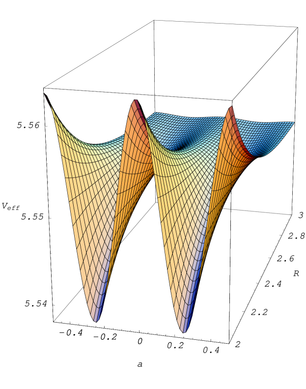
Figure 1: Effective potential as a function of $a$, for $2\leq R\leq 3$ in units of $10^{-4}M_{s}^{4}$.

The mass term at the origin, in the limit $r\to\infty$ and for arbitrary $R$, can be equally computed from Eq. (4) using the Poisson resummation (5). The result is:

$$\mu^{2}(R)=-\varepsilon^{2}(R)\,g^{2}\,M_{s}^{2}$$ (9)

with

$$\varepsilon^{2}(R)={1\over 2\pi^{2}}\int_{0}^{\infty}\frac{dl}{\left(2\,l\right)^{5/2}}{\theta_{2}^{4}\over 4\eta^{12}}\left(il+{1\over 2}\right)R^{3}\sum_{n}n^{2}e^{-2\pi n^{2}R^{2}l}\ .$$ (10)

The parameter $\varepsilon$ is plotted in Fig. 2 as a function of $R$ in a typical range $1/4<R<5$.

Figure 2: The parameter $\varepsilon$ in (10) as a function of $R$ in $\alpha^{\prime}$ units.

At the lower end, it has almost reached its asymptotic value for $R\to 0$ , $\varepsilon(0)\simeq 0.14$, and the effective cutoff for the mass term at the origin is $M_{s}$, as can be seen from Eq. (9). At large $R$, $\mu^{2}(R)$ falls off as $1/R^{2}$, which is the effective cutoff in the limit $R\to\infty$, in agreement with field theory results in the presence of a compactified extra dimension [11] . In fact, in the limit $R\to\infty$ an analytic approximation to $\varepsilon(R)$ can be computed as,

$$\varepsilon(R)\simeq\frac{\varepsilon_{\infty}}{M_{s}\,R}\,,\qquad\qquad\varepsilon_{\infty}^{2}=\frac{3\,\zeta(5)}{4\,\pi^{4}}\simeq 0.008\,,$$ (11)

which approximately describes Fig. 2 for large values of $R$.

Notice that the mass term (9) we found for the Wilson line $a$ also applies, by gauge invariance, to the charged massless fields which belong to the same representation.

Electroweak symmetry breaking

In the previous example we obtained a VEV of the order of the string scale, because we only considered Wilson lines, which correspond to tree-level flat directions in the Cartan subalgebra of the gauge group, and have put to zero the VEV’s of all other fields. Thus, the total potential to be minimized appeared at the one-loop level. Had we minimized the effective potential with respect to fields charged under the Cartan subalgebra, we would have found the same solution (which corresponds to a true minimum in the multidimensional field space) since the charged fields acquire, from the Wilson lines, positive tree-level squared masses and have vanishing VEV’s. In more realistic models, the Wilson lines are at least partially projected away by an orbifold projection which also breaks the gauge group. If the orbifold projection acts in a supersymmetric way, as was the case of the $Z_{2}$ in the previous example, the calculation of the squared mass term remains valid for the left-over charged scalars in the spectrum, up to an overall numerical factor given by the order of the orbifold group ($1/N$ for a $Z_{N}$ orbifold). Moreover, the charged scalars have a tree-level potential which can be obtained by an appropriate truncation, dictated by the orbifold, of a supersymmetric theory. These two facts allow the existence of a (local) perturbative minimum, around which higher order terms in the expansion of the one loop potential can be neglected since the charged scalars would acquire a VEV controlled by the quadratic terms.

We will illustrate these points within the context of the toy model described in the previous section. The crucial property is that the bosonic sector of the non-supersymmetric D$\bar{5}$ branes is identical to the one of an $N=2$ supersymmetric theory obtained by a $Z_{2}$ orbifold projection from an $N=4$ theory based on a “fictitious” $USp(32)$ gauge group. The latter contains six adjoint scalars that can be organized in three $N=1$ chiral multiplets $\Phi_{i}$ with $i=1,2,3$. Notice that in this model supersymmetry is explicitly broken because the fermions belong to the antisymmetric instead of the adjoint (symmetric) representation of $USp(32)$. The $Z_{2}$ projection breaks $USp(32)$ into $USp(16)\times USp(16)$ and keeps the adjoint of $USp(16)\times USp(16)$ from $\Phi_{1}$ and the $\bf{(16,16)}$ components from $\Phi_{2,3}$. The tree-level scalar potential can be obtained straightforwardly by a corresponding truncation of the potential of the $N=4$ theory:

$$V_{N=4}=\frac{g^{2}}{2}{\rm Tr}\left(\sum_{i,j}\left|\left[\Phi_{i},\Phi_{j}\right]\right|^{2}+\left(\sum_{i}\left[\Phi_{i},\Phi_{i}^{\dagger}\right]\right)^{2}\right)\,.$$ (12)

The result is identical to the potential of an $N=2$ theory with $USp(16)\times USp(16)$ gauge group and one hypermultiplet in the $\bf{(16,16)}$ representation. In $N=1$ notation, it corresponds to the superpotential $W=g/\sqrt{2}\ \varphi_{2}\varphi_{1}\varphi_{3}$ where $\varphi_{1}$ is the adjoint from $\Phi_{1}$ and $\varphi_{2,3}$ are the two bifundamental chiral multiplets from $\Phi_{2,3}$. The $F$- and $D$-term contributions to the potential come from the first and second term of Eq. (12), respectively.

As we discussed in detail after Eq. (2), the $Z_{2}$ orbifold projection does not by itself break all supersymmetries and does not play any role in the computation of the potential. As a result, the scalar mass terms generated at one loop receive contributions only from the untwisted sector which treats the adjoint and the $\bf{(16,16)}$ scalars in the same way, as an adjoint of $USp(32)$. Thus, the generated masses of the different scalars can be obtained from the same functional of the radii through permutations. In particular, this means that scalars describing displacement of branes in dimensions of the same size acquire equal masses. For instance, in the isotropic 3-brane limit of six large transverse dimensions, $r\to\infty$ and $R\to 0$, the result (9) applies for all scalar components.

We would like now to discuss possible phenomenological applications of these results. Let us assume that there is a sequence of “supersymmetric” orbifold projections that lead to the Standard Model living on some non-supersymmetric brane configuration along the line of the toy model presented above. In the minimal case, where there is only one Higgs doublet $h$ originating from the untwisted sector, the scalar potential would be:

$$V=\lambda(h^{\dagger}h)^{2}+\mu^{2}(h^{\dagger}h)\,,$$ (13)

where $\lambda$ arises at tree-level and is given by an appropriate truncation of a supersymmetric theory. Within the minimal spectrum of the Standard Model, $\lambda=(g_{2}^{2}+g^{\prime 2})/8$, with $g_{2}$ and $g^{\prime}$ the $SU(2)$ and $U(1)_{Y}$ gauge couplings, as in the MSSM. On the other hand, $\mu^{2}$ is generated at one loop and can be estimated by Eqs. (9) and (10).

The potential (13) has a minimum at $\langle h\rangle=(0,v/\sqrt{2})$, where $v$ is the VEV of the neutral component of the $h$ doublet, fixed by $v^{2}=-\mu^{2}/\lambda$. Using the relation of $v$ with the $Z$ gauge boson mass, $M_{Z}^{2}=(g_{2}^{2}+g^{\prime 2})v^{2}/4$, and the fact that the quartic Higgs interaction is provided by the gauge couplings as in supersymmetric theories, one obtains for the Higgs mass a prediction which is the MSSM value for $\tan\beta\to\infty$ and $m_{A}\to\infty$:

$$M_{h}=M_{Z}\ .$$ (14)

Furthermore, one can compute $M_{h}$ in terms of the string scale $M_{s}$, as $M_{h}^{2}=-2\mu^{2}=2\varepsilon^{2}g^{2}M_{s}^{2}$, or equivalently

$$M_{s}=\frac{M_{h}}{\sqrt{2}\,g\varepsilon}$$ (15)

The lowest order relations (14) and (15) receive in general two kinds of higher order corrections. On the one hand, there might be important string corrections that we will discuss in the next section. On the other hand, from the point of view of the effective field theory, they are valid at the string scale $M_{s}$, and Standard Model radiative corrections should be taken into account for scales between $M_{s}$ and $M_{Z}$. In particular, the tree level Higgs mass has been shown to receive important radiative corrections from the top-quark sector. For present experimental values of the top-quark mass, the Higgs mass in Eqs. (14) and (15) is raised to values around 120 GeV [9]. Moreover from Eq. (15), we can compute the string scale $M_{s}$. There is a first ambiguity in the value of the gauge coupling $g$ at $M_{s}$, which depends on the details of the model. Here, we use a typical unification value $g\simeq 1/\sqrt{2}$. A second ambiguity concerns the numerical coefficient $\varepsilon$ which is in general model dependent. In our calculation, this is partly reflected in its $R$-dependence, as seen in Fig. 2. Varying $R$ from 0 to 5, that covers the whole range of values for a transverse dimension $1<1/R<\infty$, as well as a reasonable range for a longitudinal dimension $1<R\mathrel{\lower 2.5pt\vbox{\hbox{$<$}\hbox{$\sim$}}}5$, one obtains $M_{s}\simeq 1-5$ TeV. Note that in the $R\gg 1$ (large longitudinal dimension) region our theory is effectively cutoff by $1/R$ and the Higgs mass is then related to it by,

$$\frac{1}{R}=\frac{M_{h}}{\sqrt{2}\,g\,\varepsilon_{\infty}}\,.$$ (16)

Using now the value for $\varepsilon_{\infty}$ in the present model, Eq. (11), we find $1/R\mathrel{\lower 2.5pt\vbox{\hbox{$>$}\hbox{$\sim$}}}1$ TeV.

A further model dependence of $\varepsilon$ comes from the order of the orbifold group. As mentioned above, had we considered a higher order orbifold, e.g. $Z_{2N}$ instead of $Z_{2}$ as required by more realistic models, $\varepsilon$ would decrease by a factor $\sqrt{N}$. As a result, the radiative electroweak symmetry breaking can be consistent with a string scale as heavy as ${\cal O}(10)$ TeV and a compactification scale $1/R\mathrel{\lower 2.5pt\vbox{\hbox{$>$}\hbox{$\sim$}}}2$ TeV.

In a more general context, the Higgs sector may be more complicated and the scalar potential could have classically undetermined flat directions as discussed in the introduction. For concreteness we will consider the case of two Higgs doublets $h_{1}$ and $h_{2}$ with a tree-level potential, obtained by an appropriate truncation of a supersymmetric theory, and equal to that of the MSSM. We are also assuming two different one-loop generated squared mass terms $\mu_{1}^{2}$ and $\mu_{2}^{2}$ for the Higgs fields:

$$V=\lambda\left(\left|h_{1}\right|^{2}-\left|h_{2}\right|^{2}\right)^{2}+\rho\left|h_{1}^{*}h_{2}\right|^{2}+\mu_{1}^{2}\left|h_{1}\right|^{2}+\mu_{2}^{2}\left|h_{2}\right|^{2}$$ (17)

where $\lambda=(g_{2}^{2}+g^{\prime 2})/8$ and $\rho=g_{2}^{2}/2$. The conditions for having a stable minimum are $\mu_{1}^{2}+\mu_{2}^{2}>0$ and $\mu_{1}^{2}\mu_{2}^{2}<0$. These conditions are fulfilled provided that one of the masses, say $\mu_{2}^{2}$, is negative and the other, say $\mu_{1}^{2}$, is positive. In this case we get the VEV’s $\langle h_{1}\rangle=0$ and $\langle h_{2}\rangle=(0,v/\sqrt{2})$, where $v^{2}=-\mu_{2}^{2}/\lambda$. Using again the relation of $v$ with $M_{Z}$, we obtain the tree-level Higgs mass spectrum :

$$M_{h_{2}}=M_{Z}\,,\qquad M_{h_{1}^{0}}^{2}=\mu_{1}^{2}+\mu_{2}^{2}\,,\qquad M_{h_{1}^{-}}^{2}=M_{h_{1}^{0}}^{2}+M_{W}^{2}\,,$$ (18)

where $h_{2}$ corresponds to the Standard Model Higgs, and $h_{1}^{0}$, $h_{1}^{-}$ to the neutral and charged components of the $h_{1}$ doublet. Moreover, the string scale is given by

$$M_{s}=\frac{M_{h_{2}}}{\sqrt{2}\,g\varepsilon_{2}}$$ (19)

with $\mu_{2}^{2}=-\varepsilon_{2}^{2}g^{2}M_{s}^{2}$.

Again, these are tree-level relations which are subject to both string and Standard Model radiative corrections. In particular, the latter provide important contributions to the mass of the Standard Model Higgs $h_{2}$, which is increased roughly to $\sim$ 120 GeV, and accordingly to the string scale given in Eq. (19). It is interesting that we obtained the same relations as in the previous example with a single Higgs field. The difference is that there is also a left-over scalar doublet whose neutral and charged components acquire masses given in Eq. (18). As we have pointed out, in this case one needs the one-loop generated squared masses for the two scalar doublets, $\mu_{1}^{2}$, $\mu_{2}^{2}$, to be different and opposite in sign. Although our toy string example allows for different values by introducing different radii, the change in sign requires more general models, such as those obtained for instance by introducing additional pairs of branes - anti-branes [7].

Discussion on string threshold corrections

We discuss now string threshold corrections to the relations (14) and (15). These are moduli dependent and may become very important only when some radii become large compared to the string length. Otherwise, if all radii are of order one in string units, higher loop corrections are order one numbers multiplied by loop factors which are suppressed when string theory is weakly coupled. Of course, these (model dependent) corrections are needed for a detailed phenomenological analysis and could be as important as those of the MSSM that increase the Higgs mass by roughly 10%. An estimate of these corrections can be done by an explicit computation of the $a^{4}$ terms in the expansion of the potential (8). Notice though that these terms do not determine uniquely the one-loop corrections to the quartic couplings of the charged fields, partly because there are more than one gauge invariant combinations. An additional subtlety is the existence of an infrared divergence as $l\to 0$, which is due to the low energy running of the couplings and must be appropriately subtracted to obtain the string threshold corrections in a definite renormalization scheme [12].

For dimensions longitudinal to our world brane, the large radius limit leads in general the theory very rapidly to a non perturbative regime, since the (ten-dimensional) string coupling becomes strong when four-dimensional gauge couplings are of order unity. On the other hand, for large transverse dimensions, the tree-level string coupling remains perturbative (of order of the gauge couplings), and therefore their size can in principle become as large as desired. If this is the case, the decompactification limit exists, and threshold corrections are again controlled by the string coupling and are suppressed by loop factors. However, this limit does not exist in general when there are massless bulk fields that propagate in one or two transverse dimensions, and threshold corrections become very important [3].

A way to see how these large corrections to the parameters of the effective lagrangian on the brane arise, is to look at the ultraviolet open string loop diagrams as emission of massless closed strings in the bulk at the location of distant sources created by other branes or orientifold planes. This emission leads to corrections that diverge linearly or logarithmically with the size of transverse space, if there are massless closed string states propagating in one or two dimensions, respectively. The case of one large transverse dimension is similar to that of a large longitudinal one, since threshold corrections grow linearly with the radius and bring rapidly the theory to a non-perturbative regime [13]. In this case, one can fine-tune the radius to a narrow region near the string scale and the low energy parameters will be very sensitive to the initial conditions.

In the case of two large transverse dimensions, the logarithmic contributions to the parameters of the effective action on the brane are similar to those in a renormalizable theory and can be resummed as in the renormalization group improved MSSM [3]. In this analogy, the string scale $M_{s}$ plays the role of the supersymmetry breaking scale, while the size of the transverse space replaces the ultraviolet cutoff at the Planck mass, $M_{P}$. For instance, if the bulk contains $n$ large transverse dimensions of common radius $R_{\perp}$, while the remaining $6-n$ have string size, one obtains the familiar relation $M_{P}^{2}=M_{s}^{2+n}R_{\perp}^{n}$. When there are massless bulk fields propagating in two of them, like e.g. twisted moduli localized at an $n-2$ dimensional subspace, the logarithmic corrections are $\propto\log(R_{\perp}M_{s})=(2/n)\log(M_{P}/M_{s})$.

Concerning the Higgs mass considered here, such large radius dependent contributions would arise if there are bulk massless fields emitted by the Higgs at zero external momentum. The vanishing of such tree-level couplings, as for instance with bulk gravitons, implies the absence of large threshold corrections for the Higgs mass at the one-loop level. This is in agreement with our result (4) which remains finite in the decompactification limit for any number of large transverse dimensions. However, large corrections can arise at higher orders, e.g. through gravitons emitted from open string loops. While computation of such effects is out of the scope of this work, we would like to discuss the general structure of such corrections and comment on their phenomenological implications.

In the simplest case, the relevant part of the world brane action in the string frame is:

$${\cal L}_{\rm brane}=e^{-\phi}\left\{\omega^{2}|DH|^{2}+{1+\tan^{2}\theta_{W}\over 8}\omega^{4}(H^{\dagger}H)^{2}+{1\over 4}(F_{SU(2)}^{2}+\cot^{2}\theta_{W}F_{Y}^{2})\right\}-\varepsilon^{2}M_{s}^{2}\omega^{4}|H|^{2}\,,$$ (20)

where $\phi$ is the string dilaton, $\omega$ the scale factor of the four-dimensional (world brane) metric, $H$ the Higgs scalar (in the string frame) and $D$ the gauge covariant derivative. The weak angle at the string scale $\theta_{W}$ must be correctly determined in the string model. Notice that the last term has no $e^{\phi}$ dependence since it corresponds to a one loop correction. The bulk fields $\phi$ and $\omega$ are evaluated in the transverse coordinates at the position of the brane. The physical couplings $g_{2}$, $\lambda$ and the mass $\mu^{2}$ are given by

$$g_{2}=e^{\phi/2}\ ,\qquad\lambda={1+\tan^{2}\theta_{W}\over 8}\,e^{\phi}\ ,\qquad\mu^{2}=-\varepsilon^{2}e^{\phi}\omega^{2}M_{s}^{2}\,,$$ (21)

while Eq. (14) remains unchanged and the relation (15) becomes

$$M_{s}=\frac{M_{h}}{\sqrt{2}\,\varepsilon\,e^{\phi/2}\omega}\,.$$ (22)

The lowest order result (15) corresponds to the (bare) value $\omega=1$.

As we discussed above, when the bulk fields $\phi$ and $\omega$ propagate in two large transverse dimensions, they acquire a logarithmic dependence on these coordinates due to distant sources. Since the value of $\phi$ at the position of the world brane is fixed by the value of the gauge coupling in Eq. (21), the relation (14) for the Higgs mass is not affected, while Eq. (22) for the string scale is corrected by a renormalization of $\omega$ which takes the generic form:

$$\omega=1+b_{\omega}g_{2}^{2}\ln(R_{\perp}M_{s})\,,$$ (23)

where $b_{\omega}$ is a numerical coefficient. This correction is similar to a usual renormalization factor in field theory, which here is due to an infrared running in the transverse space. Depending on the sign of $b_{\omega}$, it can enhance ($b_{\omega}<0$) or decrease ($b_{\omega}>0$) the value of the string scale by the factor $1/\omega$. This effect can be important since the involved logarithm is large, varying between 7 and 35, for $R_{\perp}$ between 1 fm and 1 mm.

In more general models, there are additional bulk fields entering in the expression of low energy couplings on the brane, such as the twisted moduli localized at the orbifold fixed points. As a result, every term in the lagrangian (20) may be multiplied by a different combination of the bulk fields that acquires an independent correction, similarly to Eq. (23). Thus, in the generic case, both relations (14) and (15) may be modified by corresponding renormalization factors that are computable in every specific model. In particular, the prediction of $\sim 120$ GeV for the Higgs mass, which coincides with that of the lightest Higgs in the MSSM for large values of $\tan\beta$ and $m_{A}$, can change by this effect.

A final important question that we have not addressed in this letter is the possible signatures of Higgs production in brane world models. Previous works done in the context of the effective field theory suggest that there may be new effects, leading in general to signatures that are different from those in the Standard Model or the MSSM [14]. It will be interesting to study this issue in the framework of the non-supersymmetric type I string models we discussed here.

References

- [1] I. Antoniadis, Phys. Lett. B246 (1990) 377; E. Witten, Nucl. Phys. B471 (135) 1996; J.D. Lykken, Phys. Rev. D54 (1996) 3693.
- [2] N. Arkani-Hamed, S. Dimopoulos and G. Dvali, Phys. Lett. B429 (1998) 263; I. Antoniadis, N. Arkani-Hamed, S. Dimopoulos and G. Dvali, Phys. Lett. B436 (1998) 257.
- [3] I. Antoniadis and C. Bachas, Phys. Lett. B450 (1999) 83.
- [4] G. Shiu and S.-H.H. Tye, Phys. Rev. D58 (1998) 106007; Z. Kakushadze and S.-H.H. Tye, Nucl. Phys. B548 (1999) 180; L.E. Ibáñez, C. Muñoz and S. Rigolin, Nucl. Phys. B553 (1999) 43; I. Antoniadis and B. Pioline, Nucl. Phys. B550 (1999) 41; K. Benakli, Phys. Rev. D60 (1999) 104002; K. Benakli and Y. Oz, Phys. Lett. B472 (2000) 83.
- [5] N. Arkani-Hamed, S. Dimopoulos and G. Dvali, Phys. Rev. D59 (1999) 086004; G.F. Giudice, R. Rattazzi and J.D. Wells, Nucl. Phys. B544 (1999) 3; E.A. Mirabelli, M. Perelstein and M.E. Peskin, Phys. Rev. Lett. 82 (1999) 2236; J.L. Hewett, Phys. Rev. Lett. 82 (1999) 4765. For a recent analysis, see : S. Cullen, M. Perelstein and M.E. Peskin, hep-ph/0001166, and references therein.
- [6] I. Antoniadis, E. Dudas and A. Sagnotti, Phys. Lett. B464 (1999) 38.
- [7] G. Aldazabal and A.M. Uranga, JHEP 9910 (1999) 024; G. Aldazabal, L.E. Ibáñez and F. Quevedo, JHEP 0001 (2000) 031; C. Angelantonj, I. Antoniadis, G. D’Appollonio, E. Dudas and A. Sagnotti, hep-th/9911081.
- [8] B. Grzadkowski and J.F. Gunion, Phys. Lett. B473 (2000) 50.
- [9] J.A. Casas, J.R. Espinosa, M. Quirós and A. Riotto, Nucl. Phys. B436 (1995) 3; M. Carena, J.R. Espinosa, M. Quirós and C.E.M. Wagner, Phys. Lett. B355 (1995) 209; M. Carena, M. Quirós and C.E.M. Wagner, Nucl. Phys. B461 (1996) 407; H.E. Haber, R. Hempfling and A.H. Hoang, Z. Phys. C75 (1997) 539; M. Carena, H.E. Haber, S. Heinemeyer, W. Hollik, C.E.M. Wagner and G. Weiglein, hep-ph/0001002; J.R. Espinosa and R.-J. Zhang, JHEP 0003 (2000) 026 and hep/ph/0003246.
- [10] C. Bachas, JHEP 9811 (1998) 23; I. Antoniadis, C. Bachas and E. Dudas, Nucl. Phys. B560 (1999) 93; N. Arkani-Hamed, S. Dimopoulos and J. March-Russell, hep-th/9908146.
- [11] I. Antoniadis, S. Dimopoulos, A. Pomarol and M. Quirós, Nucl. Phys. B544 (1999) 503; A. Delgado, A. Pomarol and M. Quirós, Phys. Rev. D60 (1999) 095008.
- [12] I. Antoniadis and M. Quirós, Phys. Lett. B392 (1997) 61.
- [13] J. Polchinski and E. Witten, Nucl. Phys. B460 (1996) 525.
- [14] N. Arkani-Hamed and S. Dimopoulos, hep-ph/9811353; L. Hall and C. Kolda, Phys. Lett. B459 (1999) 213; R. Barbieri and A. Strumia, Phys. Lett. B462 (1999) 144; X.-G. He, Phys. Rev. D61 (2000) 036007; T.G. Rizzo and J.D. Wells, Phys. Rev. D61 (2000) 016007 ; A. Datta and X. Zhang, Phys. Rev. D61 (2000) 074033; G.F. Giudice, R. Rattazzi and J.D. Wells, hep-ph/0002178.